Constraints on the Epoch of Reionization with Roman Space Telescope
and the Void Probability Function of Lyman-Alpha Emitters

Abstract

We use large simulations of Lyman-Alpha Emitters with different fractions of ionized intergalactic medium to quantify the clustering of Ly$\alpha$ emitters as measured by the Void Probability function (VPF), and how it evolves under different ionization scenarios. We quantify how well we might be able to distinguish between these scenarios with a deep spectroscopic survey using the future Nancy Grace Roman Space Telescope. Since Roman will be able to carry out blind spectroscopic surveys of Ly$\alpha$ emitters continuously between $7<z<12$ to sensitivities of at least $10^{-17}$ erg sec^-1 over a wide field of view, it can measure the epoch of reionization as well as the pace of ionization of the intergalactic medium (IGM). We compare deep Roman surveys covering roughly 1, 4, and 16 deg², and quantify what constraints on reionization the VPF may find for these surveys. A survey of 1 deg² would distinguish between very late reionization and early reionization to 3$\sigma$ near $z=7.7$ with the VPF. The VPF of a 4 deg² survey can distinguish between slow vs. fast, and early vs. late, reionization at $>3-4\sigma$ at several redshifts between $7<z<9$. However, a survey of 13-16 deg² would allow the VPF to give several robust constraints ($>5-8\sigma$) across the epoch of reionization, and would yield a detailed history of the reionization of the IGM and its effect on Lyman-$\alpha$ Emitter clustering.

1 Introduction

The epoch of reionization (EoR) is the era when the earliest galaxies ionized the ultraviolet-opaque ‘fog’ of neutral hydrogen that filled the early universe. Reionization history is still not well constrained, as various probes have led to different conclusions about its timing, pace, and sources (McQuinn, 2016). Lyman-$\alpha$ emitters (LAEs), which are star-forming galaxies that strongly emit in the Ly$\alpha$ line, offer practical probes of the reionization process. Detecting LAEs by their line emission enables surveys of otherwise faint galaxies across a wide redshift range. Because the Ly$\alpha$ line is resonantly scattered, it is easily attenuated by any amount of neutral hydrogen, and its visibility is highly sensitive to the ionization state of intergalactic gas throughout the reionization process (as predicted by Miralda-Escudé 1998; Haiman & Spaans 1999).

A common method of constraining reionization with LAEs uses the Ly$\alpha$ luminosity function (LF; first implemented by Malhotra & Rhoads 2004; e.g. Ouchi et al. 2010; Santos et al. 2016; Ouchi et al. 2018; Morales et al. 2021). This works by comparing the observed Ly$\alpha$ LF to that expected in a fully ionized medium (commonly based on the observed LF at a redshift where reionization is believed to be complete, e.g. $z=5.7$, Ajiki et al. 2003; Ouchi et al. 2003; Hu et al. 2004). LAE LF studies have reached various constraints for reionization. Some report suppression of the LAE LF in ranges within $5.7<z<7$, with inferred neutral fractions of order 20–40 percent (McQuinn et al. 2007; Kashikawa et al. 2006; Iye et al. 2006; Ouchi et al. 2010; Kashikawa et al. 2011; Konno et al. 2014, 2018). Others report upper bounds on neutral IGM (Malhotra & Rhoads 2004, 2006), including some bounds that are tight enough to challenge some of the suggested detections of neutral gas whose results of $<20$–30 percent at $z=7$ are consistent with a fully ionized medium]Wold2022a. LF suppression can have causes beyond a partially reionized IGM, such as cosmic variance, the evolution of the halo mass function (Dijkstra et al., 2007), and evolution in various factors that affect which galaxies strongly emit Ly$\alpha$ (e.g. Ota et al. 2008; Stark et al. 2010; Pentericci et al. 2011; Ono et al. 2012; Schenker et al. 2012; Endsley et al. 2021; Hassan & Gronke 2021).

However, some constraints on reionization from the LAE LF conflict with those from other measurements. For example, results suggesting a mostly ionized universe at $z\sim 6$ (Fan et al. 2006 using the IGM temperature and quasar Gunn & Peterson 1965 troughs), or $z>7-8$ extended reionization (from cosmic microwave background anisotropies, Dunkley et al. 2009). Studies examining the Ly$\alpha$ emission directly find mixed results, with some suggesting moderate to very high neutral fraction in the IGM at $z\sim 7.5$ (e.g. Jung et al. 2020 v.s. Hoag et al. 2019; Mason et al. 2019), likely due to gaps in our understanding of how Ly$\alpha$ visibility during the EoR evolves in different types of galaxies and the inhomogeneity of reionization (Jung et al., 2022). Some results challengen even the the extremely early Finkelstein et al. (2019) model of reionization, such as the implied background of Ly$\alpha$ photons at $z\sim 14$ to create the 78 MHz absorption profile of EDGES (Bowman et al., 2018), and the very recent detection of a high EW LAE at $z=10.6$ using JWST (Bunker et al., 2023). There is still not a clear definitive picture of the neutral fraction of the IGM across these studies and methods; deep, blind searches for Ly$\alpha$ over large volumes offer a path to robust understanding.

The clustering of EoR LAEs is independent from the evolution of their intrinsic LF, and provides an additional method of constraining reionization to help resolve these tensions (McQuinn et al., 2007). Most constraints have used the angular two-point correlation function (Ouchi et al. 2010; Sobacchi & Mesinger 2015; Ouchi et al. 2018; Gangolli et al. 2021) or related statistics (e.g. count-in-cells in Jensen et al. 2014). In this work, we focus on the Void Probability Function (VPF), a less common choice for EoR LAEs (Kashikawa et al. 2006; McQuinn et al. 2007) but one that may offer more sensitivity than the angular correlation function under some models (Gangolli et al., 2021). The VPF quantifies clustering by measuring how likely a circle or sphere of a given size is to be empty in a galaxy sample. As the 0${}^{\text{th}}$ moment of count-in-cells, or zero-point volume-averaged correlation function, it carries the signature of higher order correlation functions. Its simplicity can be used to derive guidelines for the required density and volume of surveys (Perez et al., 2021).

In Perez et al. (2022, henceforth Paper 1), we quantify what constraints the VPF could yield for reionization when applied to large-area blind narrowband searches for LAEs, such as the Lyman-Alpha Galaxies in the Epoch of Reionization (LAGER) narrowband survey. LAGER detects $z=6.9$ LAEs using a narrowband filter centered at 9642Å with FWHM=92Å (corresponding to approximately 30 cMpc at $z=6.9$), mounted on the 3.3 deg² field-of-view DECam on Cerro Tololo’s 4-meter Blanco Telescope. So far, LAGER has yielded initial constraints of $\langle x_{i}\rangle_{v}>0.67$ with its four-field LF (Wold et al. 2022, building off Hu et al. 2019), and has the observation and analysis of another four fields in progress. Using the Jensen et al. (2014) simulations, Paper 1 identifies how well 1, 4, or 8 LAGER DECam fields distinguish different ionization fractions with the VPF, and lays out a framework and case for using the two-dimensional VPF together to constrain the ionized hydrogen fraction implied by LAE clustering.

While narrowband surveys like LAGER (Zheng et al. 2017; Hu et al. 2019, 2021; Wold et al. 2022) and SILVERRUSH (Ouchi et al. 2018; Konno et al. 2018) have been constraining the end of reionization with LAEs, the higher redshift EoR has been much more difficult to study on a large scale with LAEs. Ground-based infrared surveys are increasingly impractical at redshifts beyond $z=6.9$ (where reionization is thought to be mostly complete), both due to atmospheric OH emission creating prohibitively bright sky foreground at most wavelengths, and a steep drop in silicon detector response at 1$\mu$m that restricts searches to instruments with comparatively small fields of view. Despite these challenges, focused ground-based searches for Ly$\alpha$ at $z=7.7$ and beyond (Tilvi et al. 2020; Oesch et al. 2015; Zitrin et al. 2015) have yielded detections of Ly$\alpha$ emitters.

The Roman Space Telescope, NASA’s next flagship mission set to launch in the mid-to-late 2020’s, is an infrared telescope with a 2.4 meter Hubble-sized mirror, and a wide-field instrument with a 0.281 deg² field of view (200 times that of Hubble’s WFC3-IR). Roman’s wide-field instrument will have a slitless grism that is capable of capturing Ly$\alpha$ at $7.2<z<14$, as well as a lower-dispersion prism that will reach Ly$\alpha$ at lower redshifts ($z>6$). Roman can carry out surveys of reionization-era LAE clustering that will notably refine our understanding of the EoR, giving definitive constraints for how and when reionization occurred.

In this work, we adapt our framework from Paper 1 to make predictions for LAE clustering observations with Roman. We quantify how Roman will constrain the timing and pace of reionization given its wide field, sensitivity, and continuous redshift coverage by combining three ingredients: a model for reionization in a $\sim(600\hbox{cMpc})^{3}$ box that includes galaxy formation and radiative transfer of Ly$\alpha$ (Jensen et al., 2014); a set of reionization history models that we use to map between redshift and a given simulated neutral fraction; and instrumental sensitivity predictions based on detailed simulations of Roman grism data sets (Wold et al, in prep). We then calculate the expected VPF and its expected uncertainties for surveys covering $\sim 1$, $\sim 4$, and $\sim 16$ square degrees, at each of five neutral fractions ($\langle x_{i}\rangle_{v}=$ {0.22, 0.40, 0.485, 0.66, 0.93}), in each of three reionization scenarios (gradual; rapid and early; rapid and late). We thereby address how large a clustering survey must be to distinguish between models for reionization history.

This paper is laid out as follows. In §2, we describe the theory and simulations that support this work: the Jensen et al. (2014) simulations of LAEs through reionization in §2.1; the models for reionization we compare in §2.2; our application of the I.G.B. Wold et al. (2023, in preparation) Roman-Ly$\alpha$ grism simulations in §2.3; how we create mock Roman LAE surveys from the above in §2.4; and finally, how we apply the VPF for reionization constraints in §2.5. In §3, we explore how the VPF evolves throughout the reionization history of the universe with different survey constructions, and how precisely Roman will be able to make out the epoch and pace of reionization. In in §3.1, we first focus on comparing the models at $z\sim 7.75$ using the entire VPF as a function of clustering distance scale, VPF(R). We then focus on an ambitious 13-16 deg² survey in §3.2, and smaller 1 and 4 deg² surveys in §3.3. Appendix A shows in detail our VPF measurements. We conclude and summarize our results in §4.

2 Simulations and Methods

2.1 Large Simulations of LAEs in Partially Reionized IGM

For samples of LAEs at various ionization fractions, we use the Jensen et al. (2014, J14) simulations of LAEs, which include radiative transfer through various amounts of ionized intergalactic medium (IGM). The simulations exist for discrete volume ionized fractions of {22, 40, 48.5, 66, 78, 89, and 93} percent, corresponding to mass ionized hydrogen fractions of {30, 50, 58, 73, 83, 92, and 95} percent. We direct readers to Paper 1 for a more complete description of the J14 simulations and their properties for contexts similar to this work, but review relevant details for their assumptions for reionization (explained fully in Jensen et al. 2013). Finally, we note there has been exciting progress in improving the simulation of Ly$\alpha$ transmission during the EoR (e.g. THESAN from Smith et al. 2022 and SPHINX from Rosdahl et al. 2018, or Qin et al. 2022 with the Meraxes semi-analytic model), though reaching volumes similar to the J14 simulations with these methods remains computationally difficult.

The underlying reionization model of the J14 simulations can be summarized as an inside-out reionization history that began somewhat early and progressed at a moderate pace. They incorporated self-regulation as galaxies take part in reionization, turning off small sources of ionizing radiation once the IGM passed 10$\%$ ionization. Briefly, halos were populated with galaxies as to match key luminosity functions in Ouchi et al. (2010); each galaxy was modelled to intrinsically emit a halo mass-dependent double-peaked Ly$\alpha$ spectrum. Scattering from the IGM was incorporated using IGMTransfer based off higher resolution hydrodynamic simulations (Laursen et al., 2011; Laursen, 2011). J14 assumed that the luminosity function at $z=6.5$ from Ouchi et al. (2010) held true, and each of the ‘scenarios’ correspond to the global-mass ionized fraction of the Universe at $z=6.5$. They constructed these ‘scenarios’ by taking the single underlying reionization simulation at a given ionization fraction and scaling the halo masses until the intrinsic luminosity function matched that at $z=5.7$. We and J14 assume the intrinsic evolution of Ly$\alpha$ galaxies is modest during the rapid phases of reionization (for example, $\Delta z=0.5$ only corresponds to 65 Myr at $z=7$).

Later in this work, we redshift the LAE catalogs to reflect the redshifts different models for the EoR predict for each ionized IGM fraction (i.e. slow/fast, early/late reionization), and then consider what Roman will observe in the context of the VPF of LAEs. We primarily focus on the $\langle x_{i}\rangle_{v}$={22, 40, 48.5, 66, 93} percent ionized simulations. Most of these fractions are predicted to exist at redshifts where the Roman grism will observe Ly$\alpha$ under the models of reionization that we analyze. The most ionized volume is in particular a useful baseline of clustering, and can be compared to ground-based surveys as well as future studies with the Roman prism that will detect Ly$\alpha$ to $z>6$. Finally, we note that when we redshift the luminosities, we are maintaining the core result of the J14 simulations–-how LAEs in different fractions of ionized IGM under their model appear, and how different ionization fractions affect the large scale structure as independently of LF evolution as possible–and then incorporating the straightforward dimming due to redshift.

Finally, we note that our application of the J14 simulations here differs in one notable way from our work in Paper 1. Paper 1 specifically focused on creating predictions for the VPF of the observed LAGER $z=6.9$ LAEs, and our selection reflected this by applying a realistic LAGER-like luminosity-dependent selection and a LAE duty cycle (following Kovač et al. 2007) to yield good consistency with the observed LAGER LAE density and luminosity function. However, as we broaden our analysis to Roman observations across such a broad redshift range, where the underlying UV and Ly$\alpha$ luminosity functions have not yet been constrained with observations, we do not apply a duty cycle, and use the J14 LAE catalogs with no modifications. Once these luminosity functions are better understood (e.g. with JWST), a retroactive duty cycle can be applied to our results by scaling all predicted number densities and all log₁₀(VPF) measurements by the duty cycle.

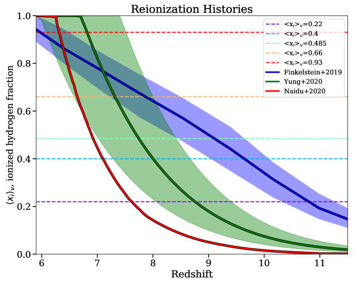
Figure 1: The predicted volume-averaged ionized hydrogen fraction by redshift according to several models of reionization: Finkelstein et al. (2019, F19, blue), Yung et al. (2020, Y20, green), and Naidu et al. (2020, N20, red). We identify at which redshift the models (solid lines) predict the ionization fractions simulated by J14 (dotted horizontal lines).

2.2 Models for Reionization

We focus on a representative sample of models for the reionization history of the universe to guide our projections for Roman. Figure 1 shows the redshift vs. volume-averaged fraction of ionized hydrogen in the IGM, according to the reionization models of Finkelstein et al. (2019, F19), Naidu et al. (2020, N20), and Yung et al. (2020, Y20) (respectively, blue, red, and green). Figure 1 shows the discrete ionization fractions of the J14 simulations as dashed horizontal lines ranging from most neutral (purple) to most ionized (red).

These models sample a range of reionization histories, driven by different assumptions about the production of ionizing photons. These models are tuned to reproduce existing constraints for reionization, such as: measurements of the IGM temperature that indicate a mostly ionized IGM at $z\sim 6$ (e.g. Fan et al. 2006); analyses of measured Ly$\alpha$ line profiles that rule out a fully neutral universe at $z=6.6$ (Haiman & Cen 2005; Ouchi et al. 2010; Rhoads et al. 2013); quasar Gunn & Peterson (1965) trough studies that find a fully ionized universe by $z=5-6$ (e.g. Fan et al. 2006; McGreer et al. 2015); and measurements of the average Thomson scattering optical depth with cosmic microwave background (CMB) anisotropies (e.g. Dunkley et al. 2009; Planck Collaboration et al. 2016) that support higher-redshift extended reionization ($z>7-8)$. These models also focus on galaxies as the likeliest and dominant sources of reionization (e.g. Robertson et al. 2013), supported by the rarity of quasars beyond $z>6$ and constraints on helium reionization (e.g. Madau & Haardt 2015). Next, we briefly describe these models for reionization.

F19 present a semi-empirical model of reionization whose core is a physically-motivated halo mass-dependent parametrization of escape fractions. In their model, the faintest galaxies in the UV collectively dominate the ionizing emissivity, leading to a reionization history that starts very early (80$\%$ volume-ionized at $z\sim 7$) and progresses at a smooth pace. They also model an AGN contribution to the end of reionization, making up one third of the budget at $z=6$, and predict a flat star formation rate density at $z>8$.

Y20 use end-to-end semi-analytic models with the goal of modeling all ionizing sources in fine detail. They use physically motivated relationships between dark matter halo formation histories and galaxy properties (including synthetic spectral energy distributions) to connect galaxy formation physics to the large-scale reionization history. They combine the Santa Cruz semi-analytic model for galaxy formation (Somerville & Primack 1999; Somerville et al. 2008, 2015) with an analytic reionization model (Madau et al. 1999, similar to that in Naidu et al. 2020), and have only the escape fraction as a free parameter.

N20 create and apply an empirical model to explore what objects carried out the bulk of ionization. Focusing specifically on ionizing photon escape fractions, their model ties the escape fraction to the star formation surface density (as motivated by recent samples of Lyman continuum leakers). Their model implies that rare very massive and UV bright galaxies (‘oligarchs’) account for the vast majority of the reionization budget.

When comparing these models purely on the reionization history they predict in Figure 1, N20 and Y20 follow a similar pattern: reionization starts very slowly and ramps up quickly after $z<8$. N20 stands out among many reionization models for how late and rapidly it occurs. F19 also stands out by presenting a reionization history that began earlier than $z>11$ and evolved slowly and steadily. In the context of LAE observations with Roman, a universe that F19 describes will find many more LAEs at higher redshifts, as the IGM has more ionized gaps that allow the photons through. On the opposite side, N20 would predict very few LAEs at $z>7$ and a mostly neutral IGM. Roman will hugely inform our understanding of reionization, with its large field-of-view and vast redshift coverage beyond the low-redshift universe where ground based observations have not found definitive constraints between these models.

2.3 Expected Roman Grism Ly$\alpha$ Response

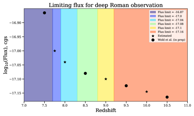
Figure 2: The redshift-dependent flux limits we use, as informed by the detailed Roman Ly$\alpha$ simulations of Wold et al. (2023, in preparation). The thresholds for applying each flux are indicated by the blocks of shaded color (shallowest at the lower redshifts in indigo, to the deepest high redshift observations in orange). Circles show the fluxes where 50$\%$ completeness of LAEs was directly simulated for a deep imaging; stars are our interpolations for redshifts in between. We treat the completeness behavior as a step-function. The fluxes applied to each redshift-reionization scenario are listed in Table LABEL:table:AllModels.

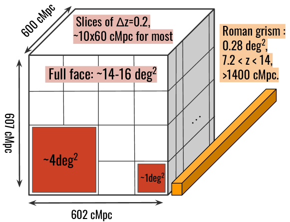
Figure 3: A schematic showing how we slice the J14 simulations to explore the constraints on reionization the Roman Space Telescope may find with the VPF. Depending on the redshift studied, the full face of the (601x607x600) cMpc³ volume corresponds to approximately 13-16 deg². For our exploration of how the VPF evolves by redshift under different models for the reionization history of the universe, we test three survey areas with Roman: the full face $\sim 16$ deg², quarter-face $\sim 4$ deg², and sixteenth-face $\sim 1$ deg². We assume a survey covering $\Delta z$=0.2, which yields between 7 to 14 equally deep slices in the simulations. For comparison, we show in yellow a long thin tube that illustrates the area and Ly$\alpha$ redshift coverage for one imaging (or, a single FOV pointing) with the Roman grism. Table LABEL:table:AllModels detail each redshift-reionization scenario’s slice depth and approximate LAE surface density.

The final step needed for our work is Roman’s expected sensitivity to Ly$\alpha$ across its broad redshift range. Here, we leverage some of the core results of Wold et al. (2023, in preparation). That work carries out detailed simulations of LAE identification in Roman grism data, and quantifies the expected completeness of LAE samples across a range of luminosity and redshift. For this work, we use the results of their deepest simulation: 25 position angles at 10 kiloseconds each, for a total of 70 hours of exposure. Wold et al. (2023, in preparation) additionally assume that a deep grism field would cover the same area as a deep broad-band field, meaning low-redshift emission line galaxies would be easily identified and lead to a very low contamination rate in the final LAE sample.

Wold et al. (2023, in preparation) test four bins for redshift completeness at $z$=7.5, 8.5, 9.5, and 10.5 for the Roman grism. They insert LAEs with known line flux and measured their recovered fraction. They have quantified what flux and Ly$\alpha$ line luminosity limits correspond to 50$\%$ completeness for various key redshifts. For $z=\{7.5,8.5,9.5,10.5\}$, the limiting fluxes are {1.4e-17, 8.3e-18, 7.5e-18, 6.9e-18} erg s^-1 cm^-2, corresponding to Ly$\alpha$ line luminosities of {9.1e+42, 7.4e+42, 8.6e+42, 9.9e+42} erg s^-1 respectively. The completeness functions approximate step functions, and we treat them as so when applying these flux selections to the unmodified J14 catalogs.

We show the redshift-dependent flux limits that we derive from Wold et al. (2023, in preparation) in Figure 2. According to these simulations, Roman reaches its deepest limiting fluxes at the highest redshifts for Ly$\alpha$. The grism is least sensitive at its blue edge (near 1 $\mu$m, or $z=7.2$ for Ly$\alpha$) but becomes much more sensitive toward redder wavelengths, reaching as deep as $\log_{10}f_{Ly\alpha}>$ -17.15 cgs for $z=10.5$. However, when also considering the increasing luminosity distance of a given LAE, we expect the Roman grism to be most sensitive to Ly$\alpha$ near $z=8.5$. Though the Roman grism will not observe any Ly$\alpha$ below $z<7.2$, the Roman prism will observe Ly$\alpha$  to $z>5.2$. Based on the results of Wold et al. (2023, in preparation) and this expected synergy between the Roman instruments, we choose to apply a ceiling sensitivity of 1.4e-17 erg s^-1 cm^-2 for all redshifts under $z<7.7$. Our assumption of this fixed flux limit at $z<7.7$ is conservative, since the prism has higher throughput than the grism at $\sim 1\mu$m.

2.4 Creating Mock LAE Samples for Various Roman Surveys

We now move to predicting the LAE clustering analyses that Roman surveys will enable, using the J14 simulated LAEs. In this section, we consider narrow slices of the J14 simulations (for a 2D VPF clustering analysis) and three different Roman survey constructions: $\sim 1$ deg², $\sim 4$ deg², or $\sim 16$ deg².

Figure 3 illustrates how we slice up the J14 volumes. We assume focused studies of depth $\Delta z\approx 0.2$, and create equal slices across the 600 cMpc volume depth. As we first implemented in Paper 1, we prioritize creating fully independent slices from the volume, for a clearer sense of the behavior of the VPF for a given area. Depending on the redshift that a given ionization model predicts an ionization fraction, there can be between 14 slices $\times$ 43 cMpc/slice (e.g. F19 predicting $\langle x_{i}\rangle_{v}=0.22$ at $z=10.8$) to 7 slices $\times$ 86 cMpc/slice (e.g. F19 predicting $\langle x_{i}\rangle_{v}=0.93$ at $z=5.95$) in the $z$-direction. The columns under ‘Slice$\times$Depth’ in Table LABEL:table:AllModels detail this for each redshift-ionization scenario.

Now armed with mock $\Delta z\approx 0.2$ slices of the J14 simulations for each reionization model and redshift scenario, we apply a redshift-dependent flux limit (Figure 2, §2.3) to the trasmitted Ly$\alpha$ luminosity of each LAE in each slice. In order to apply the Roman-specific flux limit from Figure 2 to a given LAE, we translate the given flux limit to a luminosity cut based on a given LAE’s position within the slice. In each J14 full-face slice, we imagine the center $Z$-position is at the redshift of focus, with $\Delta z\pm 0.1$ as the back and front edges of the slice. We associate the relative comoving position of a LAE in the slice to a luminosity cut, and apply the given flux limit for the central redshift in Figure 2 to generate a flux-limited samples for 2D clustering.

Next, we consider the $X$ and $Y$ dimensions of our mock LAE samples. At the redshifts examined, the full-face of the (602$\times$607) cMpc² J14 simulations cover between 13-16 deg². We split each slice into exact fourths (301$\times$303.5 cMpc²) or sixteenths (150.5$\times$151.75 cMpc²) to examine slices of approximately 4 deg² or 1 deg², respectively. This maximizes the number of completely independent mock LAE samples we are able to create, and covers a broad range of possible survey areas. Later in this work, we use all independent $\Delta z=0.2$ slices to explore the variability in the VPF as a function of survey area. Figure 3 displays our handling of the J14 simulations, with the additional illustration of what the default Roman grism will observe: an area of 0.281 deg² simultaneously covering $7.2<z<14$. Therefore, Roman will need approximately 4 independent and non-overlpaping FOV pointings to cover 1 deg², approximately 16 for 4 deg², etc. Finally, though we are artificially creating slices of $\Delta z=0.2$ about specific redshifts, in truth Roman will be able to access LAEs across the bulk of reionization history.

Table LABEL:table:AllModels summarizes the results of transforming each model into a redshift-reionization scenario for clustering measurements, including the size of the given slices, the limiting line flux applied, and resulting LAE surface density. To measure the surface density “$\Sigma$, LAEs deg^-2”, we average the number of the LAEs that pass their redshift-position flux cut across all full-face slices, and divide by the area implied for 602$\times$607 cMpc² at the central redshift. These are the LAE surface densities expected under the Wold et al. (2023, in preparation) sensitivity predictions and nuances of the J14 simulations across all our redshift-reionization scenarios, ranging from a few dozen to a few hundred deg^-2.

Table 1: Details for mock Roman observations given the Finkelstein et al. (2019, F19), Yung et al. (2020, Y20), and Naidu et al. (2020, N20) models for reionization, generated from the unmodified Jensen et al. (2014, J14) LAE catalogs. For a given $\langle x_{i}\rangle_{v}$ simulation, we list: the redshift each model predicts the ionized fraction; the number and depth of slices corresponding to $\Delta z=0.2$ depth; the flux limit applied at the redshift in log₁₀ erg sec^-1; the corresponding limiting Ly$\alpha$ line luminosity in a slice; and the average surface density in LAEs per deg² for a full-face slice.

$\langle x_{i}\rangle_{v}$	Slice Center $z$			Slices$\times$Depth, cMpc			Lim. Flux, log10 erg s-1			Lim. log10L${}_{\text{Ly}\alpha}$			$\Sigma$, LAEs deg-2
Model:	F19	Y20	N20	F19	Y20	N20	F19	Y20	N20	F19	Y20	N20	F19	Y20	N20
0.22	10.8	8.75	7.6	14x43	12x50	10x60	-17.2	-17.08	-16.9	43.04	42.91	42.98	29	52	43
0.40	9.65	8.0	7.1	13x45	10x60	9x67	-17.2	-17.04	-16.9	42.92	42.88	42.91	66	103	85
0.485	9.1	7.75	6.9	12x50	10x60	8x75	-17.1	-17.0	-16.9	42.93	42.89	42.88	104	148	160
0.66	7.85	7.3	6.65	10x60	9x67	8x75	-17.0	-16.9	-16.9	42.88	42.97	42.85	162	133	211
0.93	5.95	6.85	6.3	7x86	8x75	8x75	-16.9	-16.9	-16.9	42.73	42.9	42.79	381	200	273

2.5 Using the Void Probability Function for Reionization

The Void Probability Function (VPF) is a measurement of clustering that quantifies how likely a region of a given size is to be empty within the sample. Or, if one drops a certain number of circles of some $R$, how many are empty? It is the zero-eth moment of count-in-cells, focusing only on the cells with no galaxies, and therefore carries the signature of higher order volume-averaged clustering statistics (White 1979). Perez et al. (2021) applied an analysis of the hierarchical scaling between the VPF and higher order correlation functions (see also Conroy et al. 2005), comparing the VPF-derived volume averaged two-point correlation function and standard Landy & Szalay (1993) correlation function for simulated $3.1<z<6.6$ LAEs. They also derived theoretical descriptions for minimum and maximum distance scale guidelines for the VPF that we use in this work.

The VPF has also been leveraged specifically for reionization constraints. Kashikawa et al. (2006) and McQuinn et al. (2007) examined the ability of the VPF to constrain reionization for Subaru LAE observations at $z=6.6$. More recently, Gangolli et al. (2021) explored the constraining power of the VPF and other clustering statistics for SILVERRUSH LAEs at $z=5.7$. In Paper 1, we used the VPF to quantify what constraints on reionization the LAGER narrowband survey will be able to make at $z=6.9$ with one, four, or eight fields’ worth of imaging.

We measure the VPF using the $k$-nearest neighbors algorithm introduced in Banerjee & Abel (2021), which is notably faster than other methods. In a given slice, the transverse comoving positions of LAEs that passed the flux cut are normalized to cover e.g. $x=0-301$, $y=0-303.5$, and $z=0-60$ cMpc for a $\sim 4$ deg² slice at $z=9$. For each of several radii between 5 and 50 cMpc, we drop 100,000 random points in a slice to measure the VPF. We repeat this process 5 times to minimize sampling error, and use the average across the five samplings as the measured VPF of a given slice. When we later explore the VPF behavior of a given redshift-reionization scenario as a function of area, we will compare the mean and standard deviation of the VPF across all $\Delta z=0.2$ slices of a particular area.

For a focused statistical analysis, in this work we will primarily discuss the VPF at $R\sim 12$ cMpc. $R\sim 12$ cMpc roughly corresponds to expected scale of ionized bubbles during reionization for the redshifts we examine. The smallest visible bubbles in the Ly$\alpha$ distribution are ones that will results in a Gunn & Peterson (1965) line center optical depth of $\tau\approx 1$, and which are therefore large enough to allow sufficient transmission of Ly$\alpha$ (see Rhoads & Malhotra 2001; Rhoads 2007). The characteristic radius of these bubbles comes out to 1.2 physical megaparsec, or:

$$R_{\text{bubble}},\ \text{cMpc}=1.2\ \text{pMpc}\times(1+z).$$ (1)

The VPF is a volume-averaged clustering statistic, which in practice means that general trends are consistent between nearby distance scales. In §3.1, however, we study the VPF across all radii for the models near $z\sim 7.8$.

3 Redshift Evolution of the VPF Across Reionization

3.1 Example Focused Constraints near $7.6<z<7.9$

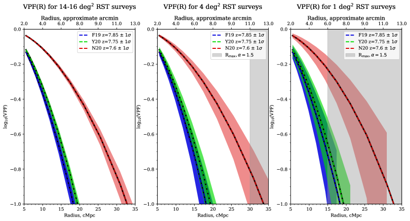
Figure 4: The complete VPF curves for the three ionization fractions–$\langle x_{i}\rangle_{v}$=0.22, 0.485, 0.66–predicted near $z\sim 7.75$ by the three models (N20, A20, F19 in red, green, blue respectively). The colored sharing are the 1$\sigma$ standard deviation across all independent $\Delta z=0.2$ slices of the given area. Grey shading indicates the approximate distance scales where the given survey area cannot measure the VPF (assuming $\alpha=1.5$, and that all models exist at $z=7.75$ for simplicity). We note that for the full-face 14-16 deg² surveys, the blue F19 and green Y20 1$\sigma$ shadings begin to overlap only at $R>15$ cMpc; and, that for the 4 deg² surveys, the mean Y20 VPF values are similar to the upper 1$\sigma$ bound of the F20 shading at nearly all distances.

To lay the framework for conceptualizing multi-redshift constraints from the VPF, let us first examine the complete VPF($R$) distribution of all our explored survey areas near just $7.6<z<7.9$. This mimics the detailed projection for the LAGER $z=6.9$ narrowband survey’s VPF we carried out in Paper 1. As Figure 1 details, each of the N20, Y20, and F19 models serendipitously correspond to one of the discrete ionization fractions of the J14 volumes around $7.6<z<7.9$. We can therefore answer: how do the complete VPF curves, for $5<R<40$ cMpc, behave for each of these distinct ionization scenarios near $7.6<z<7.9$?

Figure 4 compares the complete VPF(R) measurements for the three models in this narrow redshift window: F19 predicting $\langle x_{i}\rangle_{v}$=0.66 near $z=7.85$; Y20 predicting $\langle x_{i}\rangle_{v}$=0.485 near $z=7.7$; and N20 predicting $\langle x_{i}\rangle_{v}<$0.22 near $z=7.6$. The dashed colored lines indicate the mean VPF across all the independent $\Delta z=0.2$ slices of a given area. The colored shaded regions indicate the (log-space) errors corresponding to the 1$\sigma$ standard deviation across the slices. The drop-off of the colored shading indicates where most slices start to find VPF($R$)=0. We also show as grey shading the maximum distance scale to measure the VPF for each survey area we probe (Perez et al., 2021, given a precision to log₁₀(VPF)$>-1.5$). Since N20 predicts such a late and swift reionization, we assume the ionization fraction will be no higher than 22$\%$ near $z=7.75$, and that therefore the VPF measured for $\langle x_{i}\rangle_{v}$=0.22 near $z=7.6$ is a good approximation. Though the Roman grism becomes more sensitive past $z>7.7$, we assume that this effect would be offset by a much more neutral IGM in the N20 model.

Much like Paper 1 showed for LAGER at $z=6.9$, we find this single redshift can yield useful constraints on reionization even with small area surveys. We find similar results for $z\sim 7.7$: increasing the area of the survey yields VPF measurements that more accurately reflect the ‘true’ VPF value of the sample with lower variance. Due to this, and the results of upcoming sections, we advocate improving the VPF’s precision by increasing the continuous covered area of a single survey region, rather than combining several independent smaller survey regions of the sky (as in Paper 1 with LAGER). With a $\sim 1$ deg² survey, N20 can be well-distinguished from the Y20/F19 scenarios ($>3\sigma$), effectively ruling in or out a very late reionization history. Increasing to $\sim 4$ deg² improves the constraint notably ($>6\sigma$) and also expands the distance scales that allow this constraint (to $R<30$ cMpc). However, the Y20/F19 models cannot be distinguished until analyzing $\sim 15$ deg² ($\sim 1.5\sigma$ at $R<15$ cMpc).

Finally, we remind readers that we have focused the scope of this analysis to $7.6<z<7.9$ for two key reasons. First, we are limited to the ionized fractions of the existing J14 simulations. Second, we focus on the representative reionization models of F19, Y20, and N20, and when in cosmic history they predict each of the discrete fractions. However, once actually observing with Roman, we will find completely independent measurements of the VPF at more redshifts than we are able to probe under this analysis. As we have done in Paper 1 for LAGER, the exercise of this sub-section can be done at any redshift to constrain which J14 ionization fraction simulation’s clustering may best describe the VPF as measured in a deep Roman LAE survey. Therefore, the overall evolution of the VPF across $7.5<z<10.5$ will help confidently constrain the pacing of our universe’s reionization history.

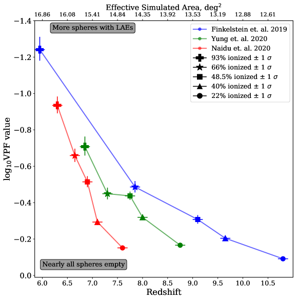
Figure 5: VPF($z$) for a Roman field covering 13-16 deg² at 11.86 cMpc. The colors indicate the model of reionization: N20 (red), F19 (blue), and Y20 (green). The shapes of the points indicate which J14 volume was used for the VPF measurement: $\langle x_{i}\rangle_{v}=$ 93 (plus sign, left-most), 66 (star), 48.5 (square), 40 (triangle), or 22 (circle, right-most) percent ionized. The effective simulated area in deg² corresponding to these slices, for a given redshift, is listed on the upper axis. Error bars correspond to the 1$\sigma$ standard deviation of the VPF across all full face $\sim 13-16$ deg² and $\Delta z=0.2$ slices created for each simulation-reionization model pairing. The detailed VPF distributions are shown in the Appendix.

3.2 Constraints from a 13-16 deg² survey

We now examine the evolution of the VPF across reionization history that Roman will observe, and identify what constraints on reionization models the VPF may yield. We focus on three representative models of reionization: the very early and slow F19 model, the quick yet middle-of-the-road Y20 model, and the very late and very fast N20 model. The complete histograms for each model’s redshift-reionization scenario VPF are shown at full scale in the Appendix A Figures 8 - 10. We ask: how well can Roman distinguish these reionization histories with the VPF using surveys of $\sim 1$ vs. $\sim 4$ vs. 13–16 deg²?

We first examine the results of the most ambitious survey we probe, for narrow slices encompassing 13-16 deg² of Roman grism observations. Figure 5 shows the VPF($z$) at $R\sim 12$ cMpc for each redshift-reionization scenario, using several independent full-face (602x607) cMpc² slices from each simulation. The 3 representative models of reionization are indicated by different colors: N20 (red), F19 (blue), and Y20 (green). The shape of each symbol indicates which J14 simulation was sliced up for the VPF measurement: 22, 40, 48.5, 66, or 93 percent ionized (marked using circles, triangles, square, stars, and crosses, respectively). The error bars are the 1$\sigma$ standard deviation across the 7-14 full-face slices’ VPFs at the given radius (some of which are smaller than the symbol sizes).

These VPF($z$) curves follow some trends: more neutral and higher-redshift slices have higher void probabilities (i.e. their $\log_{10}$(VPF) is closer to 0, meaning they have more empty dropped circles). This is not unsurprising, as lower density samples implicitly have more and larger voids. However, the pattern of the VPF also incorporates the predicted reionization histories, which Roman will be able to observe simultaneously across redshift history.

This largest explored survey area creates many opportunities for clear constraints on the timing and pace of reionization. First, we see the VPF is clearly different between different ionization fractions at the same redshift (as seen in Paper 1, and further explored for $z=7.75$ in §3.1). With the $\sim 16$ deg² survey area, the VPF of all models’ redshift-reionization scenarios are completely separated by at least 1.5$\sigma$ (e.g. F19 and Y20 near $z=7.8$), with most separated by $>4\sigma$ from the nearest scenario of another model. For example, the Y20 ($\langle x_{i}\rangle_{v}$=0.93) and the N20 ($\langle x_{i}\rangle_{v}$=0.485) VPF measurements at $z=7.8$ are distinguishable to 5$\sigma$, allowing Roman to decidedly constrain between a very late vs. somewhat early reionization. Past $z=8$, where the Roman grism reaches peak sensitivity, the F19 ($\langle x_{i}\rangle_{v}$=0.66) and Y20 ($\langle x_{i}\rangle_{v}$=0.485) may be separated enough for distinguishing constraints of 3$\sigma$ with a survey of $\sim 14$ deg². The measurement of the VPF near $z\sim 8.1$ would therefore clarify if reionization started very early or somewhat early. Additionally, the very late and fast N20 ($\langle x_{i}\rangle_{v}$=0.22) history can be distinguished from the earlier start of Y20 ($\langle x_{i}\rangle_{v}$=0.40, 0.485) or F19 ($\langle x_{i}\rangle_{v}$=0.66) to $>8\sigma$ near $z=7.75$. Finally, if the pacing and timing predicted by the F19 and Y20 VPF($z$) hold near $z\sim 9$, the Roman may distinguish the two reionization histories to more than 4$\sigma$ with the VPF.

Taken together, these results show that by combining at least two redshifts, we are able to distinguish any pair of reionization histories with the VPF of LAEs. More broadly, this VPF test will only be unable to distinguish two reionization models if they yield functionally identical reionization histories. Therefore, measurements of the Ly$\alpha$ VPF throughout the Roman grism will definitively identify which of the probed models best describes the reionization history of the universe. Additionally, we note the investment into a survey of this scale would offer other constraints on reionization, such as Ly$\alpha$-21cm cross-correlation (e.g. Hutter et al. 2019, who identified $\sim$20 deg² surveys to utilize SKA alongside the angular correlation function of LAEs).

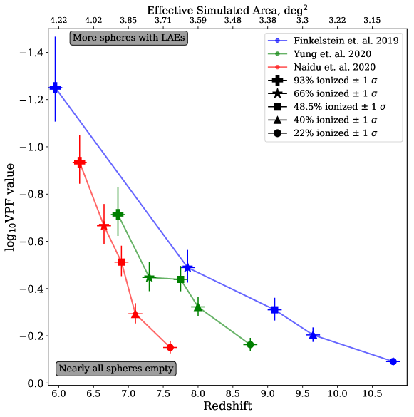
Figure 6: Like Figure 5, but instead for slices of $\sim 4$ deg² created for each simulation-reionization model pairing (at least $8\times 4$ slices, each with a redshift depth of $\Delta z=0.2$).

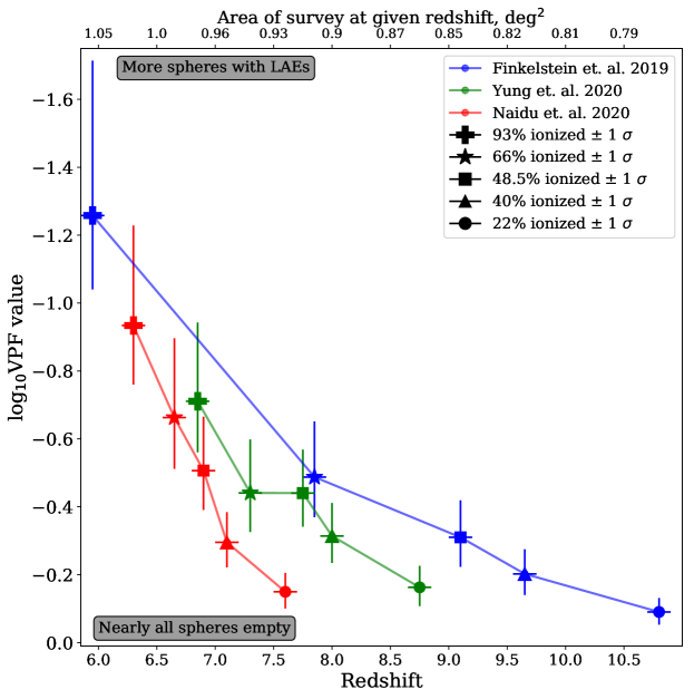
Figure 7: Like Figures 5 and 6, but instead for slices of approximately 1 deg² (one sixteenth of the face of the Jensen et al. 2014 simulations; at least 16$\times$8 total slices). Error bars are the 1$\sigma$ standard deviation across all slices’ VPF.

3.3 Constraints from 4 and 1 deg² surveys

A LAE survey of 13-16 deg² with Roman would yield excellent $>5\sigma$ constraints at several redshifts, and decisively rule in or out key features of reionization history. Might we reach similar constraints with smaller surveys? We repeat the process of Figure 6 using instead the $\sim 4$ deg² and $\sim 1$ deg² slices.

The primary effect of the smaller area is decreased precision in the VPF from Poisson noise and larger variance across slices due to the decreasing total number of LAEs. However, we find the VPF across the $\sim 4$ deg² slices can still reach multiple constraints for the epoch and pace of reionization, to between 2.5 - 8$\sigma$ across $6.8<z<9$. First, the Y20 ($\langle x_{i}\rangle_{v}$=0.93) and the N20 ($\langle x_{i}\rangle_{v}$=0.485) VPF measurements at $z\sim 6.8$ are distinguishable to about 2.5$\sigma$. This would identify a very late reionization at redshifts accessible with the Roman prism and ground-based surveys (consistent with our results in Paper 1 for LAGER). Additionally, near $z=7.5-8$ the F19 ($\langle x_{i}\rangle_{v}$=0.66) and N20 ($\langle x_{i}\rangle_{v}$=0.22) scenarios could be distinguished to 3$\sigma$ apart, independently constraining early vs. late and slow vs. fast reionization. Notably, more constraints for the timing of reionization are distinguishable to $6-8\sigma$ near $z=7.75$ between the N20 ($\langle x_{i}\rangle_{v}$=0.22) and Y20 ($\langle x_{i}\rangle_{v}$=0.40, 0.485) models. However, we note these constraints are within the redshift range where the sensitivity of the grism changes rapidly, so LAE selection must be done carefully to leverage this survey area. Finally, the F19 ($\langle x_{i}\rangle_{v}$=0.485) and Y20 ($\langle x_{i}\rangle_{v}$=0.22) scenarios at $z\sim 9$ may be at least $3-4\sigma$ apart if the apparent patterns hold beyond where the discrete fractions of the J14 simulations reach.

Is it possible to make constraints with an even smaller survey? Figure 7 repeats our process for the $\sim 1$ deg² slices at $R=11.86$ cMpc. The reduced area puts some of our earlier constraints out of reach, as fewer galaxies introduce more uncertainty to the VPF and makes fractions more difficult to distinguish. This scarcity of LAEs can still be a useful constraint: for example, an early investment of a few weeks of Roman observing time to cover 1 deg² may find fewer than 50 LAEs deg^-2 at $z>8$, which would provide some support for the later reionization models (i.e. measure a low surface density consistent with the more neutral ionization fractions). However, there are still strong constraints the VPF of LAEs will yield for the timing of reionization with a $\sim 1$ deg² survey. The N20 ($\langle x_{i}\rangle_{v}$=0.22) and Y20 ($\langle x_{i}\rangle_{v}$=0.40, 0.485) histories near $z=7.75$ are still distinguishable to $3-4\sigma$ (assuming LAE selection that accounts for the rapidly changing grism sensitivity to Ly$\alpha$). Additionally, the scenarios of F19 (near $\langle x_{i}\rangle_{v}$=0.485) and Y20 ($\langle x_{i}\rangle_{v}$=0.22) at $z\sim 9$ could perhaps be distinguished to more than $2\sigma$ apart, if the apparent trend of we see in the VPF($z$) holds.

4 Conclusion

This work explores the constraints the Roman Space Telescope will find for the timing and pace of reionization based on the clustering of LAEs. We use the Void Probability Function (VPF), which asks how many randomly dropped spheres are empty, is tied to all higher order correlation functions, and is a simple clustering statistic to implement and guide survey construction. We focus on three representative models for reionization: Finkelstein et al. (2019, very early and slow reionization), Yung et al. (2020, moderately early and quick reionization), and Naidu et al. (2020, late and very fast reionization). We analyze ($602\times 607\times 600$) cMpc³ simulations of LAEs through reionization at discrete ionized IGM fractions between $0.22<\langle x_{i}\rangle_{v}<0.93$ (Jensen et al., 2014). Informed by detailed simulations of Roman’s grism responsiveness to Ly$\alpha$ (Wold et al. in prep), we create flux-limited mock LAE samples as may be observed by Roman throughout reionization.

We mimic the three models’ reionization histories by redshifting each J14 simulation to the redshifts where each model predicts the given volume-averaged ionization fraction. We create mock Roman LAE surveys of $\Delta z=0.2$ that cover: 13-16 deg² (the full face of the simulation), $\sim 4$ deg² (quarter face of the simulation), or $\sim 1$ deg² (one sixteenth of the simulation face). We measure the VPF and answer: what constraints on the pacing and timing of reionization might Roman find with the clustering of LAEs, as a function of survey area?

We find that a $\sim 1$ deg² survey can distinguish between very late vs. early reionization near $z=7.7$ to $>3\sigma$, and between very early and slow vs. quick and late reionization near $z\sim 9$ to $>2\sigma$. By investing in $\sim 4$ deg², the VPF of LAEs is able to distinguish: early vs. late reionization to $3\sigma$ between $7.5<z<8$ and $z\sim 9$; and slow vs. fast reionization to $3\sigma$ at $z\sim 8$. Additionally, early and slow vs. fast and late reionization may be distinguished to $6\sigma$ or more near $z=7.5-8$. Finally, we find a 13-16 deg² area would give VPF measurements that would essentially trace out a precise reionization history of the universe, and determine with great confidence ($>4-5\sigma$) the most accurate model describing the timing and pace of reionization.

Appendix A Detailed VPF distributions

What do the distributions of the VPF across all the independent $\Delta z=0.2$ slices look like for each redshift-reionization scenario? We compare the distribution of the VPF measurements across: the ‘full-face’ slices of approximately 13-16 deg² (top row), the few dozen slices of approximately 4 deg² (middle row), and the several dozen slices of approximately 1 deg² (bottom row) in Figures 8 - 10. Columns indicate the J14 volume analyzed in the scenario, with the most neutral to the left and increasing in ionization fraction. Each figure shows, in a solid line whose color corresponds to the $\langle x_{i}\rangle_{v}$ value of the simulation (e.g. in Figure 1, the mean of the VPF across the several full-face slices). The histograms for the 4 deg² and 1 deg² slices also show the 1$\sigma$ standard deviation across the full face slices. Increasing the survey area steeply narrows the distribution of sampled slices about what is likely the true VPF value.

The histograms are not normalized, and we use (5, 15, 20) default-Matplotlib bins for the ($\sim 16$, $\sim 4$, $\sim 1$) deg² slices. We also remind readers that each slices’ VPF measurement is the average across 5 calculations of the VPF with the Banerjee & Abel (2021) $k$-NN method. Though not shown here, all valid distributions are clustered compared to random (e.g. Paper 1 Figures). Finally, a quirk of the VPF is that the spread of a distribution is related to its central value: more clustered VPFs (closer to zero) also have narrower distributions.

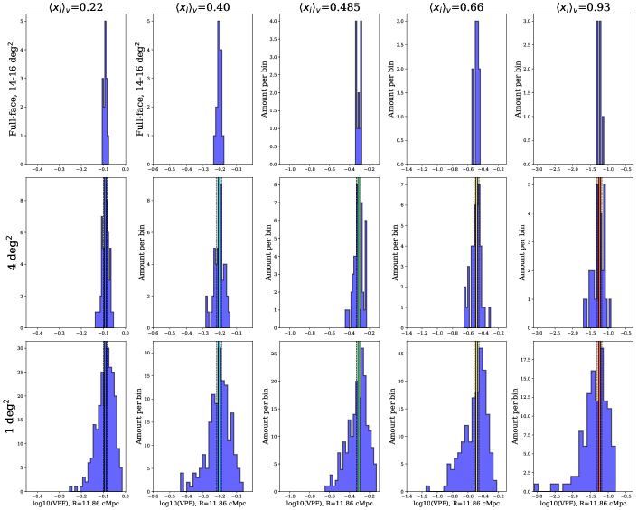
Figure 8: Focused distributions of the VPF measured at $R=11.86$ cMpc for the Finkelstein et al. (2019) redshift-reionization scenarios; the columns are the J14 simulation volume (left: $\langle x_{i}\rangle_{v}$=0.22, in increasing order until right: $\langle x_{i}\rangle$=0.93). The rows are for the Roman survey area probed: full-face 13-16 deg² (top), $\sim 4$ deg² (middle), $\sim 1$ deg² (bottom). The solid lines in all figures indicate the mean VPF across the full-face slices; the semi-transparent shading in the $\sim 4$ deg² and $\sim 1$ deg² histograms are the 1$\sigma$ standard deviation measured on the full-face distributions.

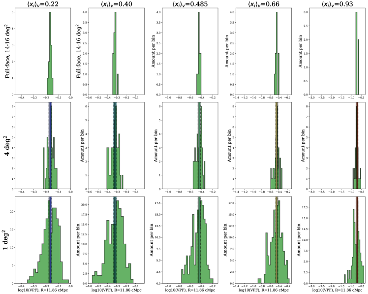
Figure 9: Like Figure 8, but for Yung et al. (2020).

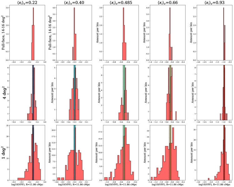
Figure 10: Like Figure 8, but for Naidu et al. (2020).

References

- Ajiki et al. (2003) Ajiki, M., Taniguchi, Y., Fujita, S. S., et al. 2003, AJ, 126, 2091, doi: 10.1086/378481
- Banerjee & Abel (2021) Banerjee, A., & Abel, T. 2021, MNRAS, 500, 5479, doi: 10.1093/mnras/staa3604
- Bowman et al. (2018) Bowman, J. D., Rogers, A. E. E., Monsalve, R. A., Mozdzen, T. J., & Mahesh, N. 2018, Nature, 555, 67, doi: 10.1038/nature25792
- Bunker et al. (2023) Bunker, A. J., Saxena, A., Cameron, A. J., et al. 2023, arXiv e-prints, arXiv:2302.07256, doi: 10.48550/arXiv.2302.07256
- Conroy et al. (2005) Conroy, C., Coil, A. L., White, M., et al. 2005, ApJ, 635, 990, doi: 10.1086/497682
- Dijkstra et al. (2007) Dijkstra, M., Wyithe, J. S. B., & Haiman, Z. 2007, MNRAS, 379, 253, doi: 10.1111/j.1365-2966.2007.11936.x
- Dunkley et al. (2009) Dunkley, J., Komatsu, E., Nolta, M. R., et al. 2009, ApJS, 180, 306, doi: 10.1088/0067-0049/180/2/306
- Endsley et al. (2021) Endsley, R., Stark, D. P., Charlot, S., et al. 2021, MNRAS, 502, 6044, doi: 10.1093/mnras/stab432
- Fan et al. (2006) Fan, X., Strauss, M. A., Becker, R. H., et al. 2006, AJ, 132, 117, doi: 10.1086/504836
- Finkelstein et al. (2019) Finkelstein, S. L., D’Aloisio, A., Paardekooper, J.-P., et al. 2019, ApJ, 879, 36, doi: 10.3847/1538-4357/ab1ea8
- Gangolli et al. (2021) Gangolli, N., D’Aloisio, A., Nasir, F., & Zheng, Z. 2021, MNRAS, 501, 5294, doi: 10.1093/mnras/staa3843
- Gunn & Peterson (1965) Gunn, J. E., & Peterson, B. A. 1965, ApJ, 142, 1633, doi: 10.1086/148444
- Haiman & Cen (2005) Haiman, Z., & Cen, R. 2005, ApJ, 623, 627, doi: 10.1086/428645
- Haiman & Spaans (1999) Haiman, Z., & Spaans, M. 1999, ApJ, 518, 138, doi: 10.1086/307276
- Harris et al. (2020) Harris, C. R., Millman, K. J., van der Walt, S. J., et al. 2020, Nature, 585, 357, doi: 10.1038/s41586-020-2649-2
- Hassan & Gronke (2021) Hassan, S., & Gronke, M. 2021, ApJ, 908, 219, doi: 10.3847/1538-4357/abd554
- Hoag et al. (2019) Hoag, A., Bradač, M., Huang, K., et al. 2019, ApJ, 878, 12, doi: 10.3847/1538-4357/ab1de7
- Hu et al. (2004) Hu, E. M., Cowie, L. L., Capak, P., et al. 2004, AJ, 127, 563, doi: 10.1086/381302
- Hu et al. (2019) Hu, W., Wang, J., Zheng, Z.-Y., et al. 2019, ApJ, 886, 90, doi: 10.3847/1538-4357/ab4cf4
- Hu et al. (2021) Hu, W., Wang, J., Infante, L., et al. 2021, Nature Astronomy, doi: 10.1038/s41550-020-01291-y
- Hunter (2007) Hunter, J. 2007, Matplotlib: A 2D Graphics Environment, doi: 10.1109/MCSE.2007.55
- Hutter et al. (2019) Hutter, A., Dayal, P., Malhotra, S., et al. 2019, BAAS, 51, 57. https://arxiv.org/abs/1903.03628
- Iye et al. (2006) Iye, M., Ota, K., Kashikawa, N., et al. 2006, Nature, 443, 186, doi: 10.1038/nature05104
- Jensen et al. (2014) Jensen, H., Hayes, M., Iliev, I. T., et al. 2014, MNRAS, 444, 2114, doi: 10.1093/mnras/stu1600
- Jensen et al. (2013) Jensen, H., Laursen, P., Mellema, G., et al. 2013, MNRAS, 428, 1366, doi: 10.1093/mnras/sts116
- Jung et al. (2020) Jung, I., Finkelstein, S. L., Dickinson, M., et al. 2020, ApJ, 904, 144, doi: 10.3847/1538-4357/abbd44
- Jung et al. (2022) Jung, I., Papovich, C., Finkelstein, S. L., et al. 2022, ApJ, 933, 87, doi: 10.3847/1538-4357/ac6fe7
- Kashikawa et al. (2006) Kashikawa, N., Shimasaku, K., Malkan, M. A., et al. 2006, ApJ, 648, 7, doi: 10.1086/504966
- Kashikawa et al. (2011) Kashikawa, N., Shimasaku, K., Matsuda, Y., et al. 2011, ApJ, 734, 119, doi: 10.1088/0004-637X/734/2/119
- Konno et al. (2014) Konno, A., Ouchi, M., Ono, Y., et al. 2014, ApJ, 797, 16, doi: 10.1088/0004-637X/797/1/16
- Konno et al. (2018) Konno, A., Ouchi, M., Shibuya, T., et al. 2018, PASJ, 70, S16, doi: 10.1093/pasj/psx131
- Kovač et al. (2007) Kovač, K., Somerville, R. S., Rhoads, J. E., Malhotra, S., & Wang, J. 2007, ApJ, 668, 15, doi: 10.1086/520668
- Landy & Szalay (1993) Landy, S. D., & Szalay, A. S. 1993, ApJ, 412, 64, doi: 10.1086/172900
- Laursen (2011) Laursen, P. 2011, IGMtransfer: Intergalactic Radiative Transfer Code. http://ascl.net/1101.003
- Laursen et al. (2011) Laursen, P., Sommer-Larsen, J., & Razoumov, A. O. 2011, ApJ, 728, 52, doi: 10.1088/0004-637X/728/1/52
- Madau & Haardt (2015) Madau, P., & Haardt, F. 2015, ApJ, 813, L8, doi: 10.1088/2041-8205/813/1/L8
- Madau et al. (1999) Madau, P., Haardt, F., & Rees, M. J. 1999, ApJ, 514, 648, doi: 10.1086/306975
- Malhotra & Rhoads (2004) Malhotra, S., & Rhoads, J. E. 2004, ApJ, 617, L5, doi: 10.1086/427182
- Malhotra & Rhoads (2006) —. 2006, ApJ, 647, L95, doi: 10.1086/506983
- Mason et al. (2019) Mason, C. A., Fontana, A., Treu, T., et al. 2019, MNRAS, 485, 3947, doi: 10.1093/mnras/stz632
- McGreer et al. (2015) McGreer, I. D., Mesinger, A., & D’Odorico, V. 2015, MNRAS, 447, 499, doi: 10.1093/mnras/stu2449
- McQuinn (2016) McQuinn, M. 2016, ARA&A, 54, 313, doi: 10.1146/annurev-astro-082214-122355
- McQuinn et al. (2007) McQuinn, M., Hernquist, L., Zaldarriaga, M., & Dutta, S. 2007, MNRAS, 381, 75, doi: 10.1111/j.1365-2966.2007.12085.x
- Miralda-Escudé (1998) Miralda-Escudé, J. 1998, ApJ, 501, 15, doi: 10.1086/305799
- Morales et al. (2021) Morales, A. M., Mason, C. A., Bruton, S., et al. 2021, ApJ, 919, 120, doi: 10.3847/1538-4357/ac1104
- Naidu et al. (2020) Naidu, R. P., Tacchella, S., Mason, C. A., et al. 2020, ApJ, 892, 109, doi: 10.3847/1538-4357/ab7cc9
- Oesch et al. (2015) Oesch, P. A., van Dokkum, P. G., Illingworth, G. D., et al. 2015, ApJ, 804, L30, doi: 10.1088/2041-8205/804/2/L30
- Ono et al. (2012) Ono, Y., Ouchi, M., Mobasher, B., et al. 2012, ApJ, 744, 83, doi: 10.1088/0004-637X/744/2/83
- Ota et al. (2008) Ota, K., Iye, M., Kashikawa, N., et al. 2008, ApJ, 677, 12, doi: 10.1086/529006
- Ouchi et al. (2003) Ouchi, M., Shimasaku, K., Furusawa, H., et al. 2003, ApJ, 582, 60, doi: 10.1086/344476
- Ouchi et al. (2010) —. 2010, ApJ, 723, 869, doi: 10.1088/0004-637X/723/1/869
- Ouchi et al. (2018) Ouchi, M., Harikane, Y., Shibuya, T., et al. 2018, PASJ, 70, S13, doi: 10.1093/pasj/psx074
- Pentericci et al. (2011) Pentericci, L., Fontana, A., Vanzella, E., et al. 2011, ApJ, 743, 132, doi: 10.1088/0004-637X/743/2/132
- Perez et al. (2022) Perez, L. A., Malhotra, S., Rhoads, J. E., Laursen, P., & Wold, I. G. B. 2022, ApJ, 940, 102, doi: 10.3847/1538-4357/ac9b57
- Perez et al. (2021) Perez, L. A., Malhotra, S., Rhoads, J. E., & Tilvi, V. 2021, ApJ, 906, 58, doi: 10.3847/1538-4357/abc88b
- Planck Collaboration et al. (2016) Planck Collaboration, Ade, P. A. R., Aghanim, N., et al. 2016, A&A, 594, A13, doi: 10.1051/0004-6361/201525830
- Qin et al. (2022) Qin, Y., Wyithe, J. S. B., Oesch, P. A., et al. 2022, MNRAS, 510, 3858, doi: 10.1093/mnras/stab3733
- Rhoads (2007) Rhoads, J. E. 2007, arXiv e-prints, arXiv:0708.2909. https://arxiv.org/abs/0708.2909
- Rhoads & Malhotra (2001) Rhoads, J. E., & Malhotra, S. 2001, ApJ, 563, L5, doi: 10.1086/338477
- Rhoads et al. (2013) Rhoads, J. E., Malhotra, S., Stern, D., et al. 2013, ApJ, 773, 32, doi: 10.1088/0004-637X/773/1/32
- Robertson et al. (2013) Robertson, B. E., Furlanetto, S. R., Schneider, E., et al. 2013, ApJ, 768, 71, doi: 10.1088/0004-637X/768/1/71
- Rosdahl et al. (2018) Rosdahl, J., Katz, H., Blaizot, J., et al. 2018, MNRAS, 479, 994, doi: 10.1093/mnras/sty1655
- Santos et al. (2016) Santos, S., Sobral, D., & Matthee, J. 2016, MNRAS, 463, 1678, doi: 10.1093/mnras/stw2076
- Schenker et al. (2012) Schenker, M. A., Stark, D. P., Ellis, R. S., et al. 2012, ApJ, 744, 179, doi: 10.1088/0004-637X/744/2/179
- Smith et al. (2022) Smith, A., Kannan, R., Garaldi, E., et al. 2022, MNRAS, 512, 3243, doi: 10.1093/mnras/stac713
- Sobacchi & Mesinger (2015) Sobacchi, E., & Mesinger, A. 2015, MNRAS, 453, 1843, doi: 10.1093/mnras/stv1751
- Somerville et al. (2008) Somerville, R. S., Hopkins, P. F., Cox, T. J., Robertson, B. E., & Hernquist, L. 2008, MNRAS, 391, 481, doi: 10.1111/j.1365-2966.2008.13805.x
- Somerville et al. (2015) Somerville, R. S., Popping, G., & Trager, S. C. 2015, MNRAS, 453, 4337, doi: 10.1093/mnras/stv1877
- Somerville & Primack (1999) Somerville, R. S., & Primack, J. R. 1999, MNRAS, 310, 1087, doi: 10.1046/j.1365-8711.1999.03032.x
- Stark et al. (2010) Stark, D. P., Ellis, R. S., Chiu, K., Ouchi, M., & Bunker, A. 2010, MNRAS, 408, 1628, doi: 10.1111/j.1365-2966.2010.17227.x
- Tilvi et al. (2020) Tilvi, V., Malhotra, S., Rhoads, J. E., et al. 2020, ApJ, 891, L10, doi: 10.3847/2041-8213/ab75ec
- Virtanen et al. (2020) Virtanen, P., Gommers, R., Oliphant, T. E., et al. 2020, Nature Methods, 17, 261, doi: 10.1038/s41592-019-0686-2
- White (1979) White, S. D. M. 1979, MNRAS, 186, 145, doi: 10.1093/mnras/186.2.145
- Wold et al. (2022) Wold, I. G. B., Malhotra, S., Rhoads, J., et al. 2022, ApJ, 927, 36, doi: 10.3847/1538-4357/ac4997
- Wright (2006) Wright, E. L. 2006, PASP, 118, 1711, doi: 10.1086/510102
- Yung et al. (2020) Yung, L. Y. A., Somerville, R. S., Finkelstein, S. L., et al. 2020, MNRAS, 496, 4574, doi: 10.1093/mnras/staa1800
- Zheng et al. (2017) Zheng, Z.-Y., Wang, J., Rhoads, J., et al. 2017, ApJ, 842, L22, doi: 10.3847/2041-8213/aa794f
- Zitrin et al. (2015) Zitrin, A., Labbé, I., Belli, S., et al. 2015, ApJ, 810, L12, doi: 10.1088/2041-8205/810/1/L12