Quantum quenches in driven-dissipative quadratic fermionic systems with parity-time symmetry

Abstract

We study the quench dynamics of noninteracting fermionic quantum many-body systems that are subjected to Markovian drive and dissipation and are described by a quadratic Liouvillian which has parity-time (PT) symmetry. In recent work, we have shown that such systems relax locally to a maximum entropy ensemble that we have dubbed the PT-symmetric generalized Gibbs ensemble (PTGGE), in analogy to the generalized Gibbs ensemble that describes the steady state of isolated integrable quantum many-body systems after a quench. Here, using driven-dissipative versions of the Su-Schrieffer-Heeger (SSH) model and the Kitaev chain as paradigmatic model systems, we corroborate and substantially expand upon our previous results. In particular, we confirm the validity of a dissipative quasiparticle picture at finite dissipation by demonstrating light cone spreading of correlations and the linear growth and saturation to the PTGGE prediction of the quasiparticle-pair contribution to the subsystem entropy in the PT-symmetric phase. Further, we introduce the concept of directional pumping phases, which is related to the non-Hermitian topology of the Liouvillian and based upon qualitatively different dynamics of the dual string order parameter and the subsystem fermion parity in the SSH model and the Kitaev chain, respectively: Depending on the postquench parameters, there can be pumping of string order and fermion parity through both ends of a subsystem corresponding to a finite segment of the one-dimensional lattice, through only one end, or there can be no pumping at all. We show that transitions between dynamical pumping phases give rise to a new and independent type of dynamical critical behavior of the rates of directional pumping, which are determined by the soft modes of the PTGGE.

I Introduction

Quantum quenches are a paradigmatic scenario for inducing and studying far-from-equilibrium dynamics in isolated quantum many-body systems. In a quantum quench, an initial state, often chosen to be the ground state of a prequench Hamiltonian, is evolved in time with a postquench Hamiltonian [1, 2]. Of particular interest are quenches across phase boundaries, which can lead to a variety of intriguing phenomena, especially in systems with nontrivial topology [3, 4, 5, 6, 7, 8, 9]. But the two basic questions that underlie the interest in nonequilibrium dynamics induced by quantum quenches read as follows: Does a given system equilibrate after a quench, i.e., do expectation values of local observables reach a steady state? And what is the nature of this steady state? It is well established that integrable quantum many-body systems, which are characterized by an extensive set of integrals of motion, relax locally to a statistical ensemble determined by the principle of maximum entropy [10]—the generalized Gibbs ensemble (GGE) [11, 12, 13, 14, 15, 16, 17]. The GGE can be regarded as being universal in the sense that its general structure is model-independent, whereas specific model-dependent details enter the GGE only through the form of the integrals of motion and as Lagrangian multipliers, the values of which are determined by the state in which the system is prepared before the quench. In this way, the GGE conserves an extensive amount of information about the initial state. Relaxation to the GGE is accompanied by a number of universal characteristic features, such as light cone propagation of correlations [16, 18], linear growth and volume-law saturation of the subsystem entropy [19, 20, 21, 22] and the equilibration of local order parameters [16, 17, 13, 14, 15].

In stark contrast, open many-body quantum systems, which are subjected to Markovian drive and dissipation, generally approach a highly model-dependent steady state that is determined by the interplay between internal Hamiltonian dynamics and the coupling to external reservoirs [23, 24, 25, 26, 27, 28, 29, 30, 31, 32]. Through these couplings, the system can exchange energy and particles with the reservoirs, breaking conservation laws the system would have in isolation. In particular, for integrable systems, this generically means that local integrals of motions of an isolated system are not conserved anymore if the system is open. As a result, after a quench, all memory of the initial state fades away with time, and the steady state takes the form of a GGE only in the limit of weak coupling $\gamma$ between the system and its environment [33, 34, 35, 36]. Yet, as we have shown in Ref. [37], the universal principles governing generalized thermalization after a quantum quench in an isolated integrable system do apply—in suitably generalized form—to specific driven-dissipative systems even for finite system-bath coupling $\gamma$; and further, key signatures, such as a driven-dissipative quasiparticle picture [38, 39, 40] and equilibration of local observables, still accompany relaxation to a maximum entropy ensemble. This unexpected robustness of generalized thermalization is ensured by parity-time (PT) symmetry of the Liouvillian that generates the dynamics of these driven-dissipative systems. To highlight the fundamental roles that are played by PT symmetry and the principle of maximum entropy, we have dubbed the ensemble such systems locally relax to the PT-symmetric GGE (PTGGE) [37].

Originally, PT symmetry has been studied as a framework for a non-Hermitian generalization of quantum mechanics. In conventional quantum mechanics, physical observables are represented by Hermitian operators, mainly because these operators have real spectra. However, as shown in seminal work by Bender et al. [41, *Bender2008], symmetry under the combination of spatial inversion or parity and time reversal can also lead to real spectra in non-Hermitian operators. In particular, an eigenvector of a PT-symmetric non-Hermitian operator is associated with a real eigenvalue if also the eigenvector itself is PT-symmetric, i.e., invariant under the PT transformation. Eigenvectors that are not invariant under the PT transformation are said to spontaneously break PT symmetry and are associated with complex eigenvalues. Typically, if a PT-symmetric operator depends on a parameter $\gamma$ that measures the degree of non-Hermiticity such that the operator is Hermitian for $\gamma=0$, all eigenvectors are PT-symmetric and the spectrum is entirely real if $\gamma$ is sufficiently small; this situation is referred to as the PT-symmetric phase. At intermediate values of $\gamma$, in the PT-mixed phase, PT-symmetric and PT-breaking eigenvectors coexist. And for large values of $\gamma$, typically all eigenvectors spontaneously break PT symmetry. Non-Hermitian generalizations of quantum mechanics, as envisioned originally in Refs. [41, *Bender2008], are restricted to the PT-symmetric phase with a real spectrum. More recently, PT-symmetric non-Hermitian versions of paradigmatic models of condensed matter theory such as the Kitaev chain [43] have received great interest due to their unconventional topological properties, in particular, in connection with the spontaneous breaking of PT symmetry that leads to the occurrence of complex eigenvalues [44, 45, 46, 47, 48, 49, 50, 51, 52]. Here, however, we are interested in PT symmetry of a special type of non-Hermitian operator: the Liouvillian that generates the dynamics of an open quantum many-body system [53, *Prosen2012a, 55, 56, 57, 58, 59, 60, 61, 62, 63, 64, 65, 66]. The coupling to external reservoirs generically induces exponential decay, which is reflected in the spectrum of the Liouvillian being complex. On the one hand, this implies that not only the PT-symmetric but also the PT-mixed and PT-broken phases can describe quantum dynamics of driven-dissipative systems; on the other hand, this puts into question the very existence of a PT-symmetric phase, since all eigenvalues of a generic Liouvillian become real only in the limit of vanishing dissipation—we choose here the convention that the real and imaginary parts of an eigenvalue of a Liouvillian determine, respectively, the oscillation frequency and decay rate of the corresponding eigenmode. However, after a shift by a constant decay rate, the single-particle spectrum of a quadratic Liouvillian, which describes a noninteracting open quantum many-body system, can become entirely real—a property that is known as passive PT symmetry [67, 68].

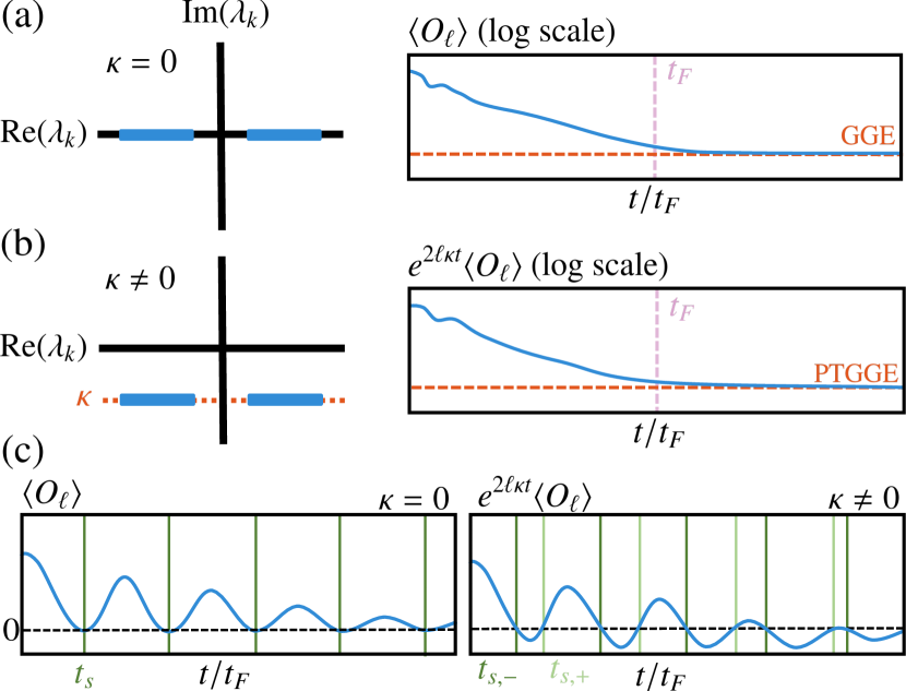
Figure 1: (a) Schematic representation of (left) the single-particle spectrum $\lambda_{k}$ of an isolated system (blue lines) with $\kappa=0$ and (right) relaxation of an observable $\langle O_{\ell}\rangle$ acting on $\ell$ sites to the GGE (red, dashed line) on a time scale $t_{F}$ (purple, dashed line). (b) For a driven-dissipative system with PT symmetry, (left) the spectrum acquires a global shift by $-i\kappa$, and (right) relaxation to the PTGGE (red, dashed line) is revealed by rescaling $\langle O_{\ell}\rangle$ with $e^{2\ell\kappa t}$. (c) Quenches from the trivial to the topological phase are accompanied by oscillatory dynamics of a topological disorder parameter are shown for (left) an isolated system, with zeros of $\langle O_{\ell}\rangle$ at multiples of a single soft-mode period $t_{s}$ (green vertical lines), and (right) a driven-dissipative system, where directional pumping is characterized by two soft-mode periods $t_{s,-}$ (dark green) and $t_{s,+}$ (light green).

Passive PT symmetry of quadratic Liouvillians is the key feature that underlies local relaxation to the PTGGE of the translationally invariant driven-dissipative fermionic lattice systems that we study below. In the PT-symmetric phase, the single-particle eigenvalues of such Liouvillians form two bands that are given by $\lambda_{\pm,k}=-i\kappa\pm\omega_{k}$, where $k$ is the quasimomentum. The momentum-independent decay rate $\kappa$ results in temporally uniform overall exponential relaxation. Independently from that, dephasing of modes with different frequencies $\omega_{k}\neq\omega_{k^{\prime}}$ leads to local relaxation to the PTGGE—this is completely analogous to isolated two-band models with single-particle dispersion $\pm\varepsilon_{k}$, where generalized thermalization to the GGE is induced by dephasing of purely oscillatory modes with $\varepsilon_{k}\neq\varepsilon_{k^{\prime}}$ [16, 69]. However, note that the PTGGE is intrinsically time-dependent due to the exponential decay at the rate $\kappa$. Relaxation of an isolated system to the GGE and of a driven-dissipative system to the PTGGE, and the underlying single-particle spectra, are illustrated in Figs. 1(a) and (b), respectively. After a quench in an isolated system, a suitably chosen observable $\langle O_{\ell}\rangle$ that acts on $\ell$ contiguous lattice sites equilibrates to the value predicted by the GGE after the Fermi time $t_{F}\sim\ell$ [14]. In contrast, after a quench to the PT-symmetric phase of a driven-dissipative system, the global shift of the spectrum by $-i\kappa$ results in exponential decay, $\langle O_{\ell}\rangle\sim e^{-2\ell\kappa t}$. Relaxation to the PTGGE through dephasing can thus be revealed by considering the rescaled expectation value $e^{2\ell\kappa t}\langle O_{\ell}\rangle$. For stronger coupling to the environment, PT symmetry is broken spontaneously and the imaginary part of $\lambda_{\pm,k}$ becomes dispersive. The long-time dynamics is then determined not by dephasing of all single-particle eigenmodes but rather by the single slowest-decaying mode that corresponds to the smallest value of $-\mathop{\mathrm{Im}}(\lambda_{\pm,k})$. Therefore, the spontaneous breaking of passive PT symmetry defines a sharp dynamical transition that delimits relaxation to the PTGGE and thus the validity of the principle of maximum entropy in driven-dissipative systems. An important caveat is that this argument for local relaxation to the PTGGE in the PT-symmetric phase is based solely on the form of the spectrum of the Liouvillian. Indeed, relaxation to the PTGGE applies as long as the overall decay with constant rate $\kappa$ causes the system to heat up to infinite temperature. Instead, for a nontrivial steady state, local relaxation to the PTGGE occurs only transiently up to a sharply-defined crossover time $t_{\times}$ [37].

In this work, we perform a detailed study of the quench dynamics and relaxation to the PTGGE of driven-dissipative fermionic many-body systems with PT symmetry, corroborating and substantially expanding upon our earlier results that we have presented in Ref. [37]. We consider two models, driven-dissipative versions of the Su-Schrieffer-Heeger (SSH) model [70, *Heeger1988] and the Kitaev chain [43], which are representative for broad classes of quadratic fermionic systems. Studying the time evolution of the dual string order parameter and the subsystem fermion parity, which serve as topological disorder parameters for the SSH model and the Kitaev chain, respectively, leads us to introduce directional pumping phases that are characterized by qualitatively different dynamics of the topological disorder parameters as illustrated in Fig. 1(c). Using the example of a Kitaev chain with long-range hopping and pairing, we show that directional pumping phases and the dynamical critical behavior at transitions between these phases are in general independent from the phases and the associated criticality that are defined in terms of PT symmetry and gap closings of the postquench Liouvillian.

This paper is organized as follows: In Sec. II, we summarize our key results. The models we study, which are driven-dissipative versions of the SSH and Kitaev chains, are introduced in Sec. III. We then establish the PTGGE as the maximum entropy ensemble for these models in Sec. IV. The spreading of correlations after a quench is studied in Sec. V, which is followed in Sec. VI by a discussion of the time evolution of the subsystem entropy. We study the dynamics of the dual string order parameter and the subsystem parity in Sec. VII, where we also introduce directional pumping phases and characterize the associated critical behavior. In Sec. VIII, we investigate directional pumping phases and phase transitions in a Kitaev chain with long-range hopping and pairing. Open research questions are presented in Sec. IX, and technical details are described in the Appendices A–E.

II Key results

We consider the following quench protocol: The system is initialized in the ground state $\lvert\psi_{0}\rangle$ of the Hamiltonian $H_{0}$ that describes an isolated SSH model or Kitaev chain, where we focus on quenches starting from the topologically trivial phases of these models. At $t=0$, a parameter of the Hamiltonian is changed abruptly; simultaneously, the system is coupled to Markovian reservoirs. The ensuing dynamics is generated by a quantum Liouvillian $\mathcal{L}$ in Lindblad form, such that the state of the system at time $t$ is given by $\rho(t)=e^{-i\mathcal{L}t}\rho_{0}$, where $\rho_{0}=\lvert\psi_{0}\rangle\langle\psi_{0}\rvert$ is the initial state. Our main results can be summarized as follows:

After quenches to the PT-symmetric phase, driven-dissipative free fermionic models relax to a maximum entropy ensemble, the parity-time symmetric generalized Gibbs ensemble (PTGGE). We have introduced the PTGGE as the maximum entropy ensemble that describes relaxation of a driven-dissipative Kitaev chain and have briefly discussed quench dynamics of an SSH model with incoherent loss and gain in Ref. [37]. Here, we present a detailed derivation of the PTGGE for the SSH model. As noted in the Introduction, dephasing of modes with different oscillation frequencies, but with a decay rate that is guaranteed to be equal for all modes by PT symmetry, is the fundamental process that underlies relaxation to the PTGGE in free fermionic systems. Due to the common decay rate of all modes, the PTGGE is inherently time-dependent. We choose the SSH model and the Kitaev chain as representatives of the two fundamental classes of quadratic fermionic systems: The isolated SSH model has a $\mathrm{U}(1)$ symmetry associated with the conservation of the number of particles, whereas due the presence of pairing terms in the isolated Kitaev chain only the fermion parity is conserved and the symmetry group is reduced to $\mathbb{Z}_{2}$. The driven-dissipative generalizations of these models combine their quadratic Hamiltonians with linear Lindblad operators, which enable the systems to exchange particles with external reservoirs and, therefore, always break particle number conservation. However, as detailed in Sec. III, we can still choose a particular form of dissipation so as to preserve a weak $\mathrm{U}(1)$ symmetry in the driven-dissipative SSH model [72]. Then, as in the isolated SSH model, no anomalous correlations are generated in the course of the dynamics. Therefore, the driven-dissipative versions of the SSH model and the Kitaev chain we consider in this work can be regarded as natural open-system generalizations of topological insulators and superconductors.

We illustrate relaxation to the PTGGE by considering the dynamics of topological disorder parameters, which take finite expectation values in the ground state in the trivial phase and vanish in the topological phase. Topological disorder parameters for the SSH model and the Kitaev chain are the dual string order parameter [73] and the subsystem fermion parity [37], respectively. The corresponding operators act nontrivially on $\ell$ contiguous lattice sites. As illustrated schematically in Fig. 1, relaxation of the topological disorder parameters to the PTGGE happens on a characteristic time scale given by the Fermi time $t_{F}\sim\ell$ [14]. We further provide analytical conjectures for the evolution of the topological disorder parameters, which we find to be in excellent agreement with our exact numerical results. These conjectures generalize analytical results for the quench dynamics of the isolated transverse field Ising model in the space-time scaling limit $\ell,t\to\infty$ with $\ell/t$ fixed [13, 14, 15], and show clearly how the dynamics are affected by drive and dissipation: Apart from the abovementioned uniform exponential decay, both the dispersion relation and the statistics of the eigenmodes of the adjoint Liouvillian, which generates the time evolution of operator expectation values, are modified, leading to pronounced quantitative differences even after rescaling of expectation values to compensate the exponential decay.

For the models we consider, a description of the late-time dynamics in terms of the PTGGE applies up to arbitrarily long times for balanced loss and gain, which leads to a steady state at infinite temperature. For a small imbalance, the PTGGE still provides an accurate description on intermediate time scales, up to a crossover time scale $t_{\times}$ that scales logarithmically with the difference between loss and gain rates. However, some observables such as the dual string order parameter are not affected at all by an imbalance between loss and gain.

Correlations show ballistic light cone spreading in the PT-symmetric phase. In contrast, after quenches to the PT-mixed and PT-broken phases, correlations spread diffusively. The single-particle spectra for isolated and PT-symmetric driven-dissipative systems shown in Figs. 1(a) and (b), respectively, suggest that PT-symmetric quadratic Liouvillians admit a notion of quasiparticles that propagate coherently with a velocity $v_{k}=d\omega_{k}/dk$, as is also the case for quasiparticle excitations of an isolated system, but have a finite lifetime $\sim 1/\kappa$. Based on this dissipative quasiparticle picture, we can expect many characteristic features of the dynamics of isolated systems to carry over to PT-symmetric driven-dissipative systems in the PT-symmetric phase. In particular, we find that the spreading of correlations after quenches to the PT-symmetric phase is described by a clear light cone structure. Interestingly, the speed at which correlations propagate is increased as compared to isolated systems; however, the finite lifetime of quasiparticles, which leads to an overall exponential decay of correlations, indicates that, in fact, it is not the case that in open systems more information is transported in a shorter time.

Light cone spreading of correlations is restricted to the PT-symmetric phase. But also after quenches to the PT-mixed and PT-broken phases there is a pronounced peak of correlations that propagates through the system. However, the peak position evolves diffusively rather than ballistically as in the PT-symmetric phase.

The growth and saturation of the subsystem entropy obeys the quasiparticle picture, adapted to driven-dissipative systems. For isolated systems, the quasiparticle picture leads to quantitative predictions for the full time evolution of the entropy of finite subsystems [19, 20, 21, 22]. One can regard the initial ground state as a source of pairs of entangled quasiparticles with opposite momenta, which propagate through the system with different velocities of at most $v_{\mathrm{max}}$. If one of the two quasiparticles that form a pair is located within the subsystem while the other one is outside of the subsystem, then this pair contributes to the entanglement between the subsystem and its complement and, therefore, to the subsystem entropy. Based on this picture, knowledge of the quasiparticle velocity and the stationary value of the subsystem entropy that is reached for $t\to\infty$ is sufficient to determine the full time evolution of the subsystem entropy in the space-time scaling limit $\ell,t\to\infty$, where $\ell$ is the size of the subsystem. The quasiparticle picture has been extended to open systems, where the requirement of ballistically propagating quasiparticles restricts its applicability to the limit of weak dissipation $\gamma\to 0$ [38, 39], and an additional contribution to the subsystem entropy due to the mixedness of the state has to be accounted for. If, however, the system under consideration has PT symmetry, then, as explained above, ballistically propagating quasiparticles exist within the entire PT-symmetric phase. Based on this observation, in Ref. [37], we have proposed an analytical conjecture for the quasiparticle-pair contribution to the subsystem entropy of a PT-symmetric Kitaev chain in the space-time scaling limit and for finite dissipation strength $\gamma$. Here, we provide further evidence for broad validity of our conjecture by applying it to the SSH model with incoherent loss and gain, where we again find excellent agreement with numerical data.

Quantum quenches in driven-dissipative systems can give rise to the unique phenomenon of directional pumping of topological disorder parameters. The time scales of directional pumping are determined by the soft modes of the PTGGE. As detailed in Sec. VII, in the isolated SSH model and the Kitaev chain, crossing the boundary between the trivial and the topological phase in the course of a quench is reflected in pumping of topological disorder parameters. That is, the dual string order parameter and the fermion parity of a subsystem of size $\ell$ exhibit oscillatory decay, crossing zero at multiplies of a time scale $t_{s}$ as illustrated in the left panel in Fig. 1(c). The period of zero crossings $t_{s}$ is determined by the momenta at which the GGE Hamiltonian vanishes—soft modes of the GGE [14, 16]. In contrast, for quenches within the trivial phase, the disorder parameters show nonoscillatory decay. Since the Hamiltonians of the SSH model and the Kitaev chain commute with the respective topological disorder parameters, processes that change the dual string order parameter and the fermion parity occur not in the bulk of the subsystem but at the interfaces between the subsystem and its complement. Interestingly, for quenches in driven-dissipative systems, the rates at which topological disorder parameters are pumped through the left and right ends of a subsystem are different. Therefore, as illustrated in the right panel in Fig. 1(c), there are two distinct time scales $t_{s,\pm}$ for zero crossings. These time scales are determined by soft modes of the PTGGE. As shown in Ref. [37] for the driven-dissipative Kitaev chain, necessary conditions for the phenomenon of directional pumping to occur are open-system dynamics leading to mixed states, and the breaking of inversion symmetry by the coupling to reservoirs.

A dynamical phase diagram can be defined in terms of directional pumping. The resulting phase boundaries and the dynamical critical behavior at these phase boundaries are, in general, different and independent from the corresponding properties defined in terms of gap closings and PT symmetry of the postquench Liouvillian. PT symmetry of the Liouvillian leads to the distinction between PT-symmetric, PT-breaking, and PT-mixed phases. For the models we consider here, the transition from the PT-symmetric to the PT-mixed phase occurs when the gap between the bands $\lambda_{\pm,k}=-i\kappa\pm\omega_{k}$ closes. Note that this corresponds to a purely dynamical phase transition that marks a qualitative change of only the coherent dynamics: As we demonstrate using the example of the density autocorrelation function, upon approaching the phase boundary from the PT-symmetric phase, a characteristic period of oscillations of local correlation functions diverges; in the PT-mixed phase, the decay of the density autocorrelation function is overdamped. Further, this transition is purely dynamical in the sense that it does not affect the steady state. Indeed, for this part of our analysis, we focus on balanced loss and gain, such that the steady state is always at infinite temperature.

Here, we show that a different and independent characterization of dynamical phases can be given in terms of directional pumping: As explained above, the pumping of topological disorder parameters for quenches from the trivial to the topological phase in isolated systems becomes directional in open systems. In particular, the topological phases of the isolated SSH model and Kitaev chain are continuously connected to phases with pumping at different rates through both ends of a subsystem. Surprisingly, we find transitions to phases with pumping through only the left or the right end of a subsystem. As the transition to such a phase is approached, one of the time scales $t_{s,\pm}$ of zero crossings diverges.

The Kitaev chain with long-range hopping and pairing represents an especially interesting model to study directional pumping phases and the associated critical behavior. In particular, we find that long-range couplings can modify the critical exponents that govern the divergence of the time scales $t_{s,\pm}$, whereas the exponents that describe the divergence of the period of oscillations of the density autocorrelation function at the gap closing at the transition from the PT-symmetric to the PT-mixed phase remain unchanged. Moreover, in the presence of long-range couplings, directional pumping phase boundaries do not always coincide with phase boundaries that are determined by gap closings, which implies that a divergence of one of the time scales $t_{s,\pm}$ does not require a gap closing in the spectrum of the Liouvillian. These findings establish directional pumping phases, phase transitions, and the associated critical behavior as new and independent concepts that are unique to quantum quenches in driven-open systems.

III Models

For the quench protocol outlined above, the postquench time evolution of the system density matrix $\rho$ is described by a Markovian quantum master equation in Lindblad form [74, *Gorini1976],

$$i\frac{d\rho}{dt}=\mathcal{L}\rho=(\mathcal{H}+i\mathcal{D})\rho,$$ (1)

where the Liouvillian $\mathcal{L}$ incorporates both unitary dynamics generated by the Hamiltonian superoperator $\mathcal{H}$ and Markovian drive and dissipation described by the dissipator $\mathcal{D}$. These superoperators are defined through their action on the density matrix $\rho$,

$$\mathcal{H}\rho =[H,\rho],$$ (2)

$$\mathcal{D}\rho =\sum_{l=1}^{L}\left(2L_{l}\rho L_{l}^{\dagger}-\{L_{l}^{\dagger}L_{l},\rho\}\right),$$ (3)

where $L_{l}$ are the quantum jump operators, describing the coupling between system and environment. In this work, we focus on noninteracting fermionic lattice models that are described by a Hamiltonian $H$ and jump operators $L_{l}$ that are quadratic and linear in fermionic operators, respectively, leading to a quadratic Liouvillian $\mathcal{L}$. For the Hamiltonian $H$, we study two models: the SSH model and the Kitaev chain, which are paradigmatic examples for a one-dimensional topological insulator and superconductor, respectively. We specify the Hamiltonians and jump operators in the following, and give a detailed description of the symmetries, spectrum, and time evolution for SSH model. For a detailed account of the driven-dissipative Kitaev chain, we refer to Ref. [37].

III.1 Driven-dissipative SSH model

The SSH model with $L$ unit cells is described by the following many-body Hamiltonian [70, *Heeger1988]:

$$H=\sum_{l=1}^{L}\left(J_{1}c_{A,l}^{\dagger}c_{B,l}+J_{2}c_{A,l+1}^{\dagger}c_{B,l}+\mathrm{H.c.}\right),$$ (4)

where $c_{s,l}$ and $c_{s,l}^{\dagger}$ are, respectively, annihilation and creation operators for fermions on sublattice $s\in\{A,B\}$ at lattice site $l$. Further, $J_{1},J_{2}\in\mathbb{R}_{>0}$ are the hopping amplitudes within and between unit cells. Unless stated otherwise, we assume periodic boundary conditions (PBC) with $c_{s,L+1}=c_{s,1}$; open boundary conditions (OBC) are implemented by setting $c_{s,L+1}=0$. We often find it convenient to parameterize $J_{1}$ and $J_{2}$ in terms of total and relative hopping amplitudes,

$$J=\frac{1}{2}\left(J_{1}+J_{2}\right),\qquad\Delta J=\frac{1}{2}\left(J_{1}-J_{2}\right).$$ (5)

As detailed below, the SSH model belongs to the Altland-Zirnbauer class BDI [76]. Therefore, the topology of the SSH model is characterized by an integer-valued invariant, the winding number $W$, and the ground state of the SSH model is topologically trivial and nontrivial for $\Delta J>0$ and $\Delta J<0$, respectively [77, 78, 79]. In this work, we study quench dynamics whereby the initial state $\lvert\psi(t)\rangle$ at $t=0$ is chosen to be the ground state $\lvert\psi_{0}\rangle$ for prequench parameters $J_{1,0}>0$ and $J_{2,0}=0$, corresponding to the topologically trivial phase. The ground state $\lvert\psi_{0}\rangle$ is Gaussian, i.e., the density matrix $\rho_{0}=\lvert\psi_{0}\rangle\langle\psi_{0}\rvert$ can be written as the exponential of a quadratic form in fermionic operators; further, since the Hamiltonian Eq. (4) is quadratic, also the time-evolved state $\rho(t)=e^{-iHt}\rho_{0}e^{iHt}$ is Gaussian [80]. Therefore, after a quench in the isolated SSH model, the state of the system is Gaussian at all times, and thus fully determined by the covariance matrix,

$$G_{l,l^{\prime}}^{s,s^{\prime}}(t)=\langle[c_{s,l},c_{s^{\prime},l^{\prime}}^{\dagger}](t)\rangle,$$ (6)

for $s,s^{\prime}\in\{A,B\}$ and $l,l^{\prime}\in\{1,\dots,L\}$, and where $\langle\cdots(t)\rangle=\mathop{\mathrm{tr}}(\cdots\rho(t))$. In particular, anomalous correlations vanish, $\langle(c_{s,l}c_{s^{\prime},l^{\prime}})(t)\rangle=\langle(c_{s,l}^{\dagger}c_{s^{\prime},l^{\prime}}^{\dagger})(t)\rangle=0$. Turning now to a driven-dissipative generalization of the SSH model, we note first that the dynamics generated by a quadratic Liouvillian $\mathcal{L}$ preserves the Gaussianity of the time-evolved mixed state $\rho(t)=e^{-i\mathcal{L}t}\rho_{0}$ [80, 81]. The vanishing of anomalous correlations, which for the isolated SSH model is a consequence of particle number conservation, can be ensured in an open SSH model by imposing the weak $\mathrm{U}(1)$ symmetry that is defined by the relation $\mathcal{L}(S\rho S^{\dagger})=S\mathcal{L}(\rho)S^{\dagger}$ for $S=e^{i\theta N}$ where the particle number operator is $N=\sum_{s\in\{A,B\}}\sum_{l=1}^{L}c_{s,l}^{\dagger}c_{s,l}$ and $\theta\in[0,2\pi)$ [72]. This weak symmetry condition guarantees that no correlations are established between Hilbert space sectors with different numbers of particles, and, therefore, anomalous correlations vanish. For the Hamiltonian part of the time evolution in Eq. (1), the weak symmetry is again a consequence of particle number conservation of the SSH Hamiltonian Eq. (4), $[H,N]=0$. A specific choice of dissipation that respects the weak $\mathrm{U}(1)$ is given by incoherent loss and gain as described by the dissipator $\mathcal{D}=\mathcal{D}_{l}+\mathcal{D}_{g}$ with

$$\begin{split}\mathcal{D}_{l}\rho&=\sum_{s\in\{A,B\}}\sum_{l=1}^{L}\left(2L_{l,s,l}\rho L_{l,s,l}^{\dagger}-\{L_{l,s,l}^{\dagger}L_{l,s,l},\rho\}\right),\\ \mathcal{D}_{g}\rho&=\sum_{s\in\{A,B\}}\sum_{l=1}^{L}\left(2L_{g,s,l}\rho L_{g,s,l}^{\dagger}-\{L_{g,s,l}^{\dagger}L_{g,s,l},\rho\}\right).\end{split}$$ (7)

The jump operators corresponding to local loss and gain are given by

$$L_{l,s,l}=\sqrt{\gamma_{l,s}}c_{s,l},\qquad L_{g,s,l}=\sqrt{\gamma_{g,s}}c_{s,l}^{\dagger},$$ (8)

where we consider loss and gain rates $\gamma_{l,s}$ and $\gamma_{g,s}$, respectively, that depend on the sublattice index. We parameterize these rates in terms of their mean and difference,

$$\gamma_{l/g}=\frac{\gamma_{l/g,A}+\gamma_{l/g,B}}{2},\qquad\Delta\gamma_{l/g}=\frac{\gamma_{l/g,A}-\gamma_{l/g,B}}{2}.$$ (9)

Below it will prove convenient to express the loss and gain rates in terms of the four independent parameters $\gamma$, $\delta$, $\Delta\gamma$, and $\Delta$, which are defined by

$$\gamma =\frac{\gamma_{l}+\gamma_{g}}{2}, \delta =\gamma_{l}-\gamma_{g},$$ (10)

$$\Delta\gamma =\frac{\Delta\gamma_{l}+\Delta\gamma_{g}}{2}, \Delta =\Delta\gamma_{l}-\Delta\gamma_{g}.$$

To determine the dynamics of the covariance matrix Eq. (6), let us first represent the jump operators in the general form

$$L_{l,l}=\sum_{l^{\prime}=1}^{2L}B_{l,l,l^{\prime}}c_{l^{\prime}},\qquad L_{g,l}=\sum_{l^{\prime}=1}^{2L}B_{g,l,l^{\prime}}c_{l^{\prime}}^{\dagger},$$ (11)

where we collect sublattice and lattice indices in a single index such that $c_{A,l}=c_{2l-1}$ and $c_{B,l}=c_{2l}$. With the $L\times 2L$ matrices $B_{l}$ and $B_{g}$, we can then introduce the bath matrices

$$M_{l}=B_{l}^{\dagger}B_{l},\qquad M_{g}=B_{g}^{{\mathchoice{\raisebox{0.0pt}{$\displaystyle\intercal$}}{\raisebox{0.0pt}{$\textstyle\intercal$}}{\raisebox{0.0pt}{$\scriptstyle\intercal$}}{\raisebox{0.0pt}{$\scriptscriptstyle\intercal$}}}}B_{g}^{*}.$$ (12)

Finally, the Liouvillian dynamics of a Gaussian state is described by the equation of motion for the covariance matrix which reads [82]

$$\frac{dG}{dt}=-i\left(ZG-GZ^{\dagger}\right)+2\left(M_{l}-M_{g}\right),$$ (13)

where the generator of the dynamics $Z$ can be interpreted as a non-Hermitian Hamiltonian and is defined by

$$Z=H-i\left(M_{l}+M_{g}\right).$$ (14)

The derivation of Eq. (13) is presented in Appendix A. In the following, we discuss some fundamental properties of the driven-dissipative SSH model. In particular, we examine symmetries of the isolated and driven-dissipative system, the corresponding spectrum and mode structure, non-Hermitian topology, and finally the dynamics of the covariance matrix.

III.1.1 Symmetries of the isolated and driven-dissipative SSH model

Symmetries of driven-dissipative systems are of fundamental importance not only for their topological classification but also—as highlighted, in particular, in our work [37]—for their quench dynamics. In our discussion of symmetries of the driven-dissipative SSH model, we will exploit translational invariance and work in momentum space. To that end, we first rewrite the Hamiltonian in Eq. (4) in terms of spinors $C_{l}=\left(c_{A,l},c_{B,l}\right)^{{\mathchoice{\raisebox{0.0pt}{$\displaystyle\intercal$}}{\raisebox{0.0pt}{$\textstyle\intercal$}}{\raisebox{0.0pt}{$\scriptstyle\intercal$}}{\raisebox{0.0pt}{$\scriptscriptstyle\intercal$}}}}$ as

$$H=\frac{1}{2}\sum_{l,l^{\prime}=1}^{L}C_{l}^{\dagger}h_{l-l^{\prime}}C_{l^{\prime}},$$ (15)

with the $2\times 2$ matrix $h_{l}=\mathbf{h}_{l}\cdot\boldsymbol{\sigma}$ where $\boldsymbol{\sigma}=(\sigma_{x},\sigma_{y},\sigma_{z})^{{\mathchoice{\raisebox{0.0pt}{$\displaystyle\intercal$}}{\raisebox{0.0pt}{$\textstyle\intercal$}}{\raisebox{0.0pt}{$\scriptstyle\intercal$}}{\raisebox{0.0pt}{$\scriptscriptstyle\intercal$}}}}$ is a vector of Pauli matrices. The momentum-space representation of the SSH model is given by the Bloch Hamiltonian $h_{k}$ that is defined as

$$h_{k}=\sum_{l=1}^{L}e^{-ikl}h_{l}=\mathbf{h}_{k}\cdot\boldsymbol{\sigma},$$ (16)

where

$$\mathbf{h}_{k}=\left(J_{1}+J_{2}\cos(k),J_{2}\sin(k),0\right)^{{\mathchoice{\raisebox{0.0pt}{$\displaystyle\intercal$}}{\raisebox{0.0pt}{$\textstyle\intercal$}}{\raisebox{0.0pt}{$\scriptstyle\intercal$}}{\raisebox{0.0pt}{$\scriptscriptstyle\intercal$}}}}.$$ (17)

Similarly, also the bath matrices in Eq. (12) can be expressed in terms of translationally invariant $2\times 2$ blocks:

$$m_{l,l}=\delta_{l,0}\begin{pmatrix}\gamma_{l,A}&0\\ 0&\gamma_{l,B}\end{pmatrix},\qquad m_{g,l}=\delta_{l,0}\begin{pmatrix}\gamma_{g,A}&0\\ 0&\gamma_{g,B}\end{pmatrix}.$$ (18)

Combining the block representations of the Hamiltonian and the bath matrices, we can write the matrix $Z$ given in Eq. (14) in the form

$$z_{l}=h_{l}-i\left(m_{l,l}+m_{g,l}\right).$$ (19)

Then, as in Eq. (16), we obtain the non-Hermitian Bloch Hamiltonian $z_{k}$ that generates the time evolution of the covariance matrix:

$$z_{k}=z_{\mathbbm{1}}\mathbbm{1}+\mathbf{z}_{k}\cdot\boldsymbol{\sigma},$$ (20)

with

$$z_{\mathbbm{1}}=-i2\gamma,\qquad\mathbf{z}_{k}=\mathbf{h}_{k}+i\mathbf{b},\qquad\mathbf{b}=-2\Delta\gamma\hat{\mathbf{e}}_{z},$$ (21)

where $\hat{\mathbf{e}}_{z}=\left(0,0,1\right)^{{\mathchoice{\raisebox{0.0pt}{$\displaystyle\intercal$}}{\raisebox{0.0pt}{$\textstyle\intercal$}}{\raisebox{0.0pt}{$\scriptstyle\intercal$}}{\raisebox{0.0pt}{$\scriptscriptstyle\intercal$}}}}$ is a unit vector along the $z$ axis.

Isolated system.

We first discuss symmetries of the isolated SSH model that is described by the Bloch Hamiltonian in Eq. (17). As stated above, the SSH model belongs to the Altland-Zirnbauer class BDI and has particle-hole symmetry (PHS), time reversal symmetry (TRS), and chiral symmetry (CS). Due to the Hermiticity of the Bloch Hamiltonian, $h_{k}=h_{k}^{\dagger}$, each of these symmetries can be expressed in two equivalent ways:

$$\begin{split}\text{PHS:}\qquad&h_{k}=-\sigma_{z}h_{-k}^{{\mathchoice{\raisebox{0.0pt}{$\displaystyle\intercal$}}{\raisebox{0.0pt}{$\textstyle\intercal$}}{\raisebox{0.0pt}{$\scriptstyle\intercal$}}{\raisebox{0.0pt}{$\scriptscriptstyle\intercal$}}}}\sigma_{z}=-\sigma_{z}h_{-k}^{*}\sigma_{z},\\ \text{TRS:}\qquad&h_{k}=h_{-k}^{{\mathchoice{\raisebox{0.0pt}{$\displaystyle\intercal$}}{\raisebox{0.0pt}{$\textstyle\intercal$}}{\raisebox{0.0pt}{$\scriptstyle\intercal$}}{\raisebox{0.0pt}{$\scriptscriptstyle\intercal$}}}}=h_{-k}^{*},\\ \text{CS:}\qquad&h_{k}=-\sigma_{z}h_{k}\sigma_{z}=-\sigma_{z}h_{k}^{\dagger}\sigma_{z},\end{split}$$ (22)

which can be confirmed by using $-\sigma_{z}\boldsymbol{\sigma}\sigma_{z}=(\sigma_{x},-\sigma_{y},-\sigma_{z})^{{\mathchoice{\raisebox{0.0pt}{$\displaystyle\intercal$}}{\raisebox{0.0pt}{$\textstyle\intercal$}}{\raisebox{0.0pt}{$\scriptstyle\intercal$}}{\raisebox{0.0pt}{$\scriptscriptstyle\intercal$}}}}$ and $\mathbf{h}_{-k}=(h_{x,k},-h_{y,k},h_{z,k})^{{\mathchoice{\raisebox{0.0pt}{$\displaystyle\intercal$}}{\raisebox{0.0pt}{$\textstyle\intercal$}}{\raisebox{0.0pt}{$\scriptstyle\intercal$}}{\raisebox{0.0pt}{$\scriptscriptstyle\intercal$}}}}$. Another symmetry that will play a key role in the following is inversion symmetry (IS). In real space and when expressed as a transformation of the fermionic operators $c_{s,l}$, inversion amounts to an exchange of the sublattices and a reflection across the middle of the chain, $c_{A/B,l}\mapsto c_{B/A,L+1-l}$. The combination of IS with TRS yields PT symmetry (PTS). In momentum space, IS and PTS are described by

$$\begin{split}\text{IS:}\qquad&h_{k}=\sigma_{x}h_{-k}\sigma_{x}=\sigma_{x}h_{-k}^{\dagger}\sigma_{x},\\ \text{PTS:}\qquad&h_{k}=\sigma_{x}h_{k}^{{\mathchoice{\raisebox{0.0pt}{$\displaystyle\intercal$}}{\raisebox{0.0pt}{$\textstyle\intercal$}}{\raisebox{0.0pt}{$\scriptstyle\intercal$}}{\raisebox{0.0pt}{$\scriptscriptstyle\intercal$}}}}\sigma_{x}=\sigma_{x}h_{k}^{*}\sigma_{x}.\end{split}$$ (23)

Driven-dissipative system.

For the driven-dissipative SSH model, we can regard the non-Hermitian matrix $z_{k}\neq z_{k}^{\dagger}$ in Eq. (20) as the generalization of the Bloch Hamiltonian to open systems. Of the two equivalent versions of the symmetries of the Bloch Hamiltonian $h_{k}$ stated in Eq. (22), only one of each applies to $z_{k}$:

$$\begin{split}\text{PHS${}^{\dagger}$:}\qquad&z_{k}=-\sigma_{z}z_{-k}^{*}\sigma_{z},\\ \text{TRS${}^{\dagger}$:}\qquad&z_{k}=z_{-k}^{{\mathchoice{\raisebox{0.0pt}{$\displaystyle\intercal$}}{\raisebox{0.0pt}{$\textstyle\intercal$}}{\raisebox{0.0pt}{$\scriptstyle\intercal$}}{\raisebox{0.0pt}{$\scriptscriptstyle\intercal$}}}},\\ \text{CS:}\qquad&z_{k}=-\sigma_{z}z_{k}^{\dagger}\sigma_{z}.\end{split}$$ (24)

Therefore, in the nomenclature of Ref. [83], the driven-dissipative SSH model belongs to the class $\mathrm{BDI}^{\dagger}$. Further, inversion symmetry in the form given in Eq. (23) is broken by the dissipative contributions to $z_{k}$. However, an inversion symmetry IS^† still applies to the traceless part $z_{k}^{\prime}=z_{k}-z_{\mathbbm{1}}\mathbbm{1}$ with $z_{\mathbbm{1}}$ given in Eq. (21); and by combining $\text{IS}^{\dagger}$ with $\text{TRS}^{\dagger}$ we obtain PTS of $z_{k}^{\prime}$:

$$\begin{split}\text{IS${}^{\dagger}$:}\qquad&z_{k}^{\prime}=\sigma_{x}z_{-k}^{\prime\dagger}\sigma_{x},\\ \text{PTS:}\qquad&z_{k}^{\prime}=\sigma_{x}z_{k}^{\prime\ast}\sigma_{x}.\end{split}$$ (25)

This form of a PT symmetry which applies after a shift that renders the generator of the dynamics traceless is called passive PT-symmety [67, 68, 64].

Let us now discuss the implication of PTS for the mode structure of the Liouvillian [41, *Bender2008]. The eigenvalues and eigenvectors of the shifted matrix $z_{k}^{\prime}$ are denoted by $\lambda_{\pm,k}^{\prime}=\pm\sqrt{\mathbf{z}_{k}\cdot\mathbf{z}_{k}}$ and $\lvert\psi_{\pm,k}\rangle$, respectively. Since $z_{k}^{\prime}$ and $z_{k}$ are related by a shift $z_{\mathbbm{1}}\mathbbm{1}$, they have the same eigenvectors, and their eigenvalues are related by $\lambda_{\pm,k}=\lambda_{\pm,k}^{\prime}+z_{\mathbbm{1}}$ with $z_{\mathbbm{1}}=-i2\gamma$. The PTS condition in Eq. (25) then leads to

$$z_{k}^{\prime}\sigma_{x}\lvert\psi_{\pm,k}\rangle^{*}=\lambda_{\pm,k}^{\prime\ast}\sigma_{x}\lvert\psi_{\pm,k}\rangle^{*}.$$ (26)

This implies that for any eigenvalue $\lambda_{\pm,k}^{\prime}$ of $z_{k}^{\prime}$ correpsonding to an eigenvector $\lvert\psi_{\pm,k}\rangle$, there is also an eigenvalue $\lambda_{\pm,k}^{\prime*}$ with eigenvector $\sigma_{x}\lvert\psi_{\pm,k}\rangle^{*}$. Since for a given value of $k$ there are only two eigenvalues which are related by $\lambda_{+,k}^{\prime}=-\lambda_{-,k}^{\prime}$, there are two possibilities: (i) PT-symmetric eigenmodes with $\lambda_{\pm,k}^{\prime}=\lambda_{\pm,k}^{\prime*}\in\mathbb{R}$ and $\sigma_{x}\lvert\psi_{\pm,k}\rangle^{*}=\lvert\psi_{\pm,k}\rangle$. For the eigenvalues $\lambda_{\pm,k}$ of the full matrix $z_{k}$ this implies that $\mathop{\mathrm{Im}}(\lambda_{\pm,k})=-2\gamma$ and $\mathop{\mathrm{Re}}(\lambda_{+,k})=-\mathop{\mathrm{Re}}(\lambda_{-,k})$. (ii) Alternatively, there exist PT-breaking eigenmodes with $\lambda_{\pm,k}^{\prime}=-\lambda_{\pm,k}^{\prime*}\in i\mathbb{R}$ and eigenvectors obeying $\sigma_{x}\lvert\psi_{\pm,k}\rangle^{*}=\lvert\psi_{\mp,k}\rangle$ such that $\mathop{\mathrm{Re}}(\lambda_{\pm,k})=0$ and $\mathop{\mathrm{Im}}(\lambda_{+,k})+2\gamma=-\left(\mathop{\mathrm{Im}}(\lambda_{-,k})+2\gamma\right)$. That is, the eigenvalues that are associated with PT-breaking eigenmodes are related by reflection across the line $-i2\gamma$.

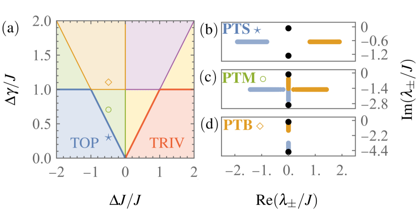
Figure 2: (a) Dynamical phase diagram of the driven-dissipative SSH model with topological phase for $\Delta J<0$ and trivial phase for $\Delta J>0$. The model features PT-symmetric (blue, red), PT-broken (orange, purple), and PT-mixed phases (green, yellow). Examples of the mode structure for the three topological phases are shown for (b) the PT-symmetric (PTS), (c) the PT-mixed (PTM), and (d) the PT-broken (PTB) phases. Positive (negative) bands are represented by orange (blue) dots and edge modes for a system with OBC by black dots. Star, circle and diamond markers in (a) indicate parameters corresponding to the spectra shown in (b)–(d).

Depending on the symmetry of the eigenvectors $\lvert\psi_{\pm,k}\rangle$ under the PT transformation, we can distinguish three different phases: (i) In the PT-symmetric phase, all eigenmodes are PT-symmetric; then, eigenvalues have a constant imaginary value, while the real part is dispersive. This is shown in Fig. 2(b). (ii) In the PT-broken phase, all eigenmodes are PT-breaking, and the corresponding eigenvalues are purely imaginary and dispersive as illustrated in Fig. 2(d). (iii) Finally, in the PT-mixed phase, PT-symmetric and PT-breaking modes exist simultaneously. Therefore, as shown in Fig. 2(c), there are two sets of eigenvalues: one that is dispersive only in the real part, and one that is dispersive only in the imaginary part. The resulting dynamical phase diagram of the driven-dissipative SSH model is shown in Fig. 2(a).

III.1.2 Spectrum of the Liouvillian

We next consider the spectra of the isolated and driven-dissipative SSH models with PBC. As shown in Appendix B, the Bloch Hamiltonian $h_{k}$ Eq. (16) can be diagonalized as

$$U_{k}^{\dagger}h_{k}U_{k}=\varepsilon_{k}\sigma_{z},$$ (27)

where the unitary matrix $U_{k}$ is given by Eq. (217) after setting $\gamma=\Delta\gamma=0$, and with the single particle dispersion relation $\varepsilon_{k}$ of the isolated SSH model defined by the magnitude of the Bloch vector,

$$\varepsilon_{k}=\left\lvert\mathbf{h}_{k}\right\rvert=\sqrt{J_{1}^{2}+J_{2}^{2}+2J_{1}J_{2}\cos(k)}.$$ (28)

For future reference, we note that in terms of the fermionic operators $d_{s,k}$ defined through

$$\begin{pmatrix}d_{A,k}\\ d_{B,k}\end{pmatrix}=U_{k}^{\dagger}\begin{pmatrix}c_{A,k}\\ c_{B,k}\end{pmatrix},\qquad c_{s,k}=\frac{1}{\sqrt{L}}\sum_{l=1}^{L}e^{-ikl}c_{s,l},$$ (29)

the Hamiltonian takes the following diagonal form:

$$H=\sum_{k\in\mathrm{BZ}}\varepsilon_{k}\left(d_{A,k}^{\dagger}d_{A,k}-d_{B,k}^{\dagger}d_{B,k}\right),$$ (30)

where the Brillouin zone is $\mathrm{BZ}=\{-\pi+\Delta k,-\pi+\Delta k,\dotsc,\pi\}$ with $\Delta k=2\pi/L$. The ground state $\lvert\psi_{0}\rangle$ is obtained by filling the band with negative energy,

$$\lvert\psi_{0}\rangle=\prod_{k\in\mathrm{BZ}}d_{B,k}^{\dagger}\left|\Omega\right\rangle,$$ (31)

where $\left|\Omega\right\rangle$ is the vacuum of particles.

Applying the formalism of third quantization [84, *Prosen2010], one can show that the spectrum of the Liouvillian is determined by the eigenvalues of the matrix $z_{k}$ in essentially the same way as the spectrum of the second-quantized Hamiltonian Eq. (4) is obtained by occupying single-particle states with energies $\pm\varepsilon_{k}$. The eigenvalues of $z_{k}$, which thus can be regarded as forming the single-particle spectrum of the Liouvillian, form two bands and are given by

$$\lambda_{\pm,k}=-i2\gamma\pm\omega_{k},$$ (32)

with the dispersion relation

$$\omega_{k}=\sqrt{\varepsilon_{k}^{2}-4\Delta\gamma^{2}},$$ (33)

where $\gamma$ and $\Delta\gamma$ are defined in Eq. (10). The dispersion relation $\omega_{k}$ determines the dynamical phase diagram of the driven-dissipative SSH model in the $\Delta J$-$\Delta\gamma$ plane depicted in Fig. 2(a). In particular, different phases can be defined in terms of the gap structure of the bands $\lambda_{\pm,k}$ [83]—as we explain next, this is equivalent to the distinction of phases in terms of PT symmetry: For small values of $\Delta\gamma$, the bands are separated by a real line gap (blue, red regions in the figure); that is, $\omega_{k}>0$ for all values of $k\in\mathrm{BZ}$, with a typical complex band structure shown in Fig. 2(b). This is the PT-symmetric phase. Upon increasing the value of $\Delta\gamma$, the real line gap closes, and the spectrum of $z_{k}$ is gapless in a finite region of the $\Delta J$-$\Delta\gamma$ plane (green, yellow). Then, for a range of momenta, $\omega_{k}$ is real; for all other values of $k$, $\omega_{k}=i\kappa_{k}$ is purely imaginary, with

$$\kappa_{k}=\sqrt{4\Delta\gamma^{2}-\varepsilon_{k}^{2}}.$$ (34)

A typical band structure in this gapless or PT-mixed phase is illustrated in Fig. 2(c). The phase boundary between PT-symmetric and PT-mixed phases is determined by a critical value $\Delta\gamma_{c}$. For $\left\lvert\Delta J\right\rvert<J$, the critical value is $\Delta\gamma_{c}=\left\lvert\Delta J\right\rvert$, and for $\left\lvert\Delta J\right\rvert>J$, it is given by $\Delta\gamma_{c}=J$. At $\left\lvert\Delta J\right\rvert=J$, the dispersion is flat, $\omega_{k}=2J$, which enables a direct transition between the phase with a real line gap and the phase with an imaginary line gap or PT-broken phase (orange, purple), where $\kappa_{k}>0$ for all values of $k\in\mathrm{BZ}$. The band structure in this phase is exemplified in Fig. 2(d).

III.1.3 Non-Hermitian topology

We have already mentioned that the SSH model is in the Altland-Zirnbauer class BDI. The class BDI in one spatial dimension is topologically nontrivial and characterized by an integer-valued invariant, called the winding number $W$. For models with a real line gap, the Altland-Zirnbauer classification can be extended to non-Hermitian systems, where in the nomenclature of Ref. [83], the driven-dissipative SSH model belongs to the class $\mathrm{BDI}^{\dagger}$. Accordingly, within the blue and red regions in Fig. 2(a), which correspond to the phase with a real line gap or, equivalently, the PT-symmetric phase, the topology of the driven-dissipative Kitaev chain is characterized by a non-Hermitian generalization of the winding number. To calculate the non-Hermitian winding number, we first find the left and right eigenstates of $z_{k}$, which we denote by $\lvert\psi_{\pm,k}^{L}\rangle$ and $\lvert\psi_{\pm,k}^{R}\rangle$, respectively. By employing the representation of $z_{k}$ given in Eq. (220), we find the eigenvalue equations

$$z_{k}^{\prime}U_{k}\left|\pm\right\rangle=\lambda_{\pm,k}U_{k}\left|\pm\right\rangle,\quad\left\langle\pm\right|U_{k}^{-1}z_{k}^{\prime}=\lambda_{\pm,k}\left\langle\pm\right|U_{k}^{-1},$$ (35)

where $\left|\pm\right\rangle$ are the eigenvectors of $\sigma_{z}$ with eigenvalues $\pm 1$. The left and right eigenvectors of $z_{k}$ are thus given by

$$\lvert\psi_{\pm,k}^{L}\rangle=U_{k}^{-\dagger}\left|\pm\right\rangle,\qquad\lvert\psi_{\pm,k}^{R}\rangle=U_{k}\left|\pm\right\rangle,$$ (36)

respectively, where $U_{k}^{-\dagger}$ is the short-hand notation for the inverse of the Hermitian adjoint of $U_{k}$. We can now define a projector on the $-$ band:

$$Q_{k}=\mathbbm{1}-\lvert\psi_{-,k}^{R}\rangle\langle\psi_{-,k}^{L}\rvert-\lvert\psi_{-,k}^{L}\rangle\langle\psi_{-,k}^{R}\rvert,$$ (37)

and determine the non-Hermitian winding number by

$$W=\frac{i}{4\pi}\int_{-\pi}^{\pi}dk\mathop{\mathrm{tr}}\!\left(\Gamma Q_{k}^{-1}\frac{d}{dk}Q_{k}\right),$$ (38)

where $\Gamma=\sigma_{z}$ is the matrix that appears in the chiral symmetry condition Eq. (24) [83], and we have replaced summation of $k\in\mathrm{BZ}$ by an integral over $k\in[-\pi,\pi]$ in the thermodynamic limit $L\to\infty$. With $\{Q_{k},\sigma_{z}\}=0$, following from chiral symmetry, and $Q=Q^{\dagger}$ by definition, we find that $Q_{k}$ is off-diagonal with

$$Q_{k}=\begin{pmatrix}0&q_{k}\\ q_{k}^{*}&0\end{pmatrix},$$ (39)

and the calculation reduces to

$$W=-\frac{i}{2\pi}\int_{-\pi}^{\pi}dk\frac{1}{q_{k}}\frac{dq_{k}}{dk}.$$ (40)

In the PT-symmetric phase, we find $q_{k}=\left.-\left(J_{1}+J_{2}e^{-ik}\right)\middle/\omega_{k}\right.$, and, therefore,

$$\frac{1}{q_{k}}\frac{dq_{k}}{dk}=-i\frac{J_{2}}{J_{2}+e^{ik}J_{1}}+\frac{J_{1}J_{2}\sin(k)}{J_{1}^{2}+J_{2}^{2}-4\Delta\gamma^{2}+2J_{1}J_{2}\cos(k)}.$$ (41)

The second term on the right-hand side of this equation is an odd function of $k$ and does not contribute to the symmetric integral in Eq. (40); the first term yields

$$W=\frac{1}{2\pi}\int_{-\pi}^{\pi}dk\frac{J_{2}}{J_{2}+e^{ik}J_{1}},$$ (42)

which is solved by substituting $z=e^{ik}$ and integrating over the unit circle $\left\lvert z\right\rvert=1$. Simple poles of the integrand are located at $z_{1}=0$ and $z_{2}=-J_{2}/J_{1}$. By using the residue theorem, we obtain the result

$$W=\begin{cases}0&\text{for }\Delta J>0,\\ 1&\text{for }\Delta J<0.\end{cases}$$ (43)

This is essentially the same result as for the isolated SSH chain, but extended to the whole PT-symmetric phase. The topological PT-symmetric phase is indicated in Fig. 2(a) by the blue area with the label “TOP,” and the trivial phase by the red area with the label “TRIV.” Interestingly, while the definition of the non-Hermitian winding number is restricted to the PT-symmetric phase with a real line gap, edge modes with $\lambda_{\mathrm{edge}}=0,\,-i4\Delta\gamma$ occur in a chain with OBC when $\Delta J<0$ and for arbitrarily large values of $\Delta\gamma$, including in the PT-mixed and PT-broken phases. In Figs. 2(b), (c), and (d), edge modes are indicated with black dots. The existence of these edge modes can be understood to be a consequence of chiral symmetry [86]: Due to chiral symmetry, each sublattice supports one edge mode. But on a given sublattice, the non-Hermitian contribution to $Z$ in Eq. (14) is constant, and its presence does not affect the eigenvectors with support on that sublattice. Therefore, the edge modes of $Z$ are identical to the edge modes of the Hamiltonian $H$, and their existence is determined by the topology of $H$. This concludes our discussion of the static properties of the SSH model, and we turn now to quench dynamics, which are the main interest of our work.

III.1.4 Dynamics of the driven-dissipative SSH model

As explained at the beginning of Sec. III.1, in this work, we consider quench dynamics with the system initially prepared in the ground state given in Eq. (31), for prequench parameters $J_{1,0}>0$ and $J_{2,0}=0$ corresponding to the trivial phase. Gaussianity of this state is preserved in the time evolution generated by a quadratic Liouvillian, and, therefore, the state of the system is fully determined by the covariance matrix $G$ defined in Eq. (6), whose dynamics are described by Eq. (13). For PBC, the covariance matrix is a $2L\times 2L$ block Toeplitz matrix, which is built from $2\times 2$ blocks given by

$$g_{l-l^{\prime}}=\begin{pmatrix}\langle[c_{A,l},c_{A,l^{\prime}}^{\dagger}]\rangle&\langle[c_{A,l},c_{B,l^{\prime}}^{\dagger}]\rangle\\ \langle[c_{B,l},c_{A,l^{\prime}}^{\dagger}]\rangle&\langle[c_{B,l},c_{B,l^{\prime}}^{\dagger}]\rangle\end{pmatrix}.$$ (44)

Further, for PBC and due to translational invariance of the Hamiltonian, the Markovian baths and the chosen initial state, all matrices in Eq. (13) are block-circulant Toeplitz matrices. Therefore, the representation of the blocks of the covariance matrix in momentum space, which is obtained through a discrete Fourier transform,

$$g_{k}=\sum_{l=1}^{L}e^{-ikl}g_{l},$$ (45)

obeys the following equation of motion:

$$\frac{dg_{k}}{dt}=-i\left(z_{k}g_{k}-g_{k}z_{k}^{\dagger}\right)+y_{k},$$ (46)

with

$$y_{k}=2\left(m_{l,k}-m_{g,k}\right)=2\left(\delta\mathbbm{1}+\Delta\sigma_{z}\right),$$ (47)

where $m_{l,k}$ and $m_{g,k}$ are the momentum-space representations of the blocks of the bath matrices defined in Eq. (18). The time-evolved covariance matrix in momentum space can be split into two contributions,

$$g_{k}(t)=g_{1,k}(t)+g_{2,k}(t),$$ (48)

where

$$g_{1,k}(t) =e^{-iz_{k}t}g_{k}(0)e^{iz_{k}^{\dagger}t},$$ (49)

$$g_{2,k}(t) =\int_{0}^{t}dt^{\prime}e^{-iz_{k}\left(t-t^{\prime}\right)}y_{k}e^{iz_{k}^{\dagger}\left(t-t^{\prime}\right)}.$$ (50)

Here, $g_{1,k}(t)$ encodes information of the initial condition $g_{k}(0)$; the second contribution $g_{2,k}(t)$ has no counterpart in isolated systems and describes the approach to the steady state $\rho_{\mathrm{SS}}$ for $t\to\infty$, where $\mathcal{L}(\rho_{\mathrm{SS}})=0$.

To evaluate the initial value $g_{k}(0)$, let us first define spinors $C_{k}=\left(c_{A,k},c_{B,k}\right)^{{\mathchoice{\raisebox{0.0pt}{$\displaystyle\intercal$}}{\raisebox{0.0pt}{$\textstyle\intercal$}}{\raisebox{0.0pt}{$\scriptstyle\intercal$}}{\raisebox{0.0pt}{$\scriptscriptstyle\intercal$}}}}$ and $D_{k}=\left(d_{A,k},d_{B,k}\right)^{{\mathchoice{\raisebox{0.0pt}{$\displaystyle\intercal$}}{\raisebox{0.0pt}{$\textstyle\intercal$}}{\raisebox{0.0pt}{$\scriptstyle\intercal$}}{\raisebox{0.0pt}{$\scriptscriptstyle\intercal$}}}}$, where the operators $c_{s,k}$ and $d_{s,k}$ are defined in Eq. (29). Further, by rearranging Eq. (27) and defining an initial unit vector $\hat{\mathbf{n}}_{0,k}=h_{0,k}/\varepsilon_{0,k}$, where $h_{0,k}$ and $\varepsilon_{0,k}$ are, respectively, the Bloch Hamiltonian and the single-particle dispersion relation for prequench parameters $J_{1,0}$ and $J_{2,0}$, we find $\hat{\mathbf{n}}_{0,k}=U_{k}\sigma_{z}U_{k}^{\dagger}$. Finally, by evaluating $\langle D_{k}D_{k}^{\dagger}\rangle_{0}=\langle\psi_{0}|D_{k}D_{k}^{\dagger}|\psi_{0}\rangle=\left(\mathbbm{1}+\sigma_{z}\right)\!/2$ for the ground state $\lvert\psi_{0}\rangle$ in Eq. (31), we obtain

$$g_{k}(0)=2\langle C_{k}C_{k}^{\dagger}\rangle_{0}-\mathbbm{1}=2U_{k}\langle D_{k}D_{k}^{\dagger}\rangle_{0}U_{k}^{\dagger}-\mathbbm{1}=\hat{\mathbf{n}}_{0,k}\cdot\boldsymbol{\sigma}.$$ (51)

In particular, for our choice of prequench parameters given by $J_{1,0}>0$ and $J_{2,0}=0$, we find

$$g_{k}(0)=\sigma_{x}.$$ (52)

With this result for the initial value, and after some algebraic simplifications, a general form for the time-dependent covariance matrix can be found [37]. We first split Eqs. (49) and (50) into two contributions that are proportional to the identity and traceless, respectively,

$$\begin{split}g_{1,k}(t)&=g_{1,\mathbbm{1},k}(t)\mathbbm{1}+\mathbf{g}_{1,k}(t)\cdot\boldsymbol{\sigma},\\ g_{2,k}(t)&=g_{2,\mathbbm{1},k}(t)\mathbbm{1}+\mathbf{g}_{2,k}(t)\cdot\boldsymbol{\sigma}.\end{split}$$ (53)

In the PT-symmetric phase, the components of $g_{1,k}(t)$ read

$$g_{1,\mathbbm{1},k}(t)=-\frac{e^{-4\gamma t}}{\omega_{k}^{2}}\left(1-\cos(2\omega_{k}t)\right)\hat{\mathbf{n}}_{0,k}\cdot\left(\mathbf{h}_{k}\times\mathbf{b}\right),$$ (54)

and

$$\mathbf{g}_{1,k}(t)=e^{-4\gamma t}\left[\hat{\mathbf{n}}_{0,k}-\frac{\varepsilon_{k}^{2}}{\omega_{k}^{2}}\left(1-\cos(2\omega_{k}t)\right)\mathbf{h}_{\perp,k}\right.\\ \left.+\frac{\varepsilon_{k}}{\omega_{k}}\sin(2\omega_{k}t)\mathbf{h}_{o,k}\right],$$ (55)

where we have introduced vectors $\mathbf{h}_{\parallel,k}$ and $\mathbf{h}_{\perp,k}$ which are parallel and perpendicular to $\hat{\mathbf{n}}_{k}=\mathbf{h}_{k}/\varepsilon_{k}$, respectively, and the out-of-plane vector $\mathbf{h}_{o,k}$ that is orthogonal to both $\hat{\mathbf{n}}_{0,k}$ and $\hat{\mathbf{n}}_{k}$:

$$\mathbf{h}_{\parallel,k}=\left(\hat{\mathbf{n}}_{0,k}\cdot\hat{\mathbf{n}}_{k}\right)\hat{\mathbf{n}}_{k},\quad\mathbf{h}_{\perp,k}=\hat{\mathbf{n}}_{0,k}-\mathbf{h}_{\parallel,k},\quad\mathbf{h}_{o,k}=-\hat{\mathbf{n}}_{0,k}\times\hat{\mathbf{n}}_{k}.$$ (56)

Here, for $\hat{\mathbf{n}}_{0,k}\nparallel\hat{\mathbf{n}}_{k}$ the dynamics of $e^{4\gamma t}\mathbf{g}_{1,k}(t)$ describe an ellipse with center $\hat{\mathbf{n}}_{0,k}-\left(\varepsilon_{k}^{2}/\omega_{k}^{2}\right)\mathbf{h}_{\perp,k}$, semi-major axis $\varepsilon_{k}^{2}/\omega_{k}^{2}$ pointing along $\mathbf{h}_{\perp,k}$, and semi-minor axis $\varepsilon_{k}/\omega_{k}$ along $\mathbf{h}_{o,k}$; for an isolated system with $\gamma=\Delta\gamma=0$, this reduces to the well-known precession of $\mathbf{g}_{1,k}(t)$ around $\mathbf{h}_{k}$.

The components of $g_{1,k}(t)$ given in Eqs. (54) and (55) decay exponentially at a rate $4\gamma$. Therefore, as indicated above, the steady state, which is determined by the limit $t\to\infty$ of $g_{k}(t)$, is described by $g_{2,k}(t)$ Eq. (50). In turn, $g_{2,k}(t)$ is proportional to $y_{k}$, which vanishes for balanced loss and gain, $\delta=\Delta=0$. The vanishing of all correlations indicates that balanced loss and gain lead to a steady state at infinite temperature, $\rho_{\mathrm{SS}}=\rho_{\infty}=\mathbbm{1}/2^{2L}$. In contrast, for $\delta,\Delta\neq 0$, also $g_{2,k}(t)\neq 0$ and the steady state is nontrivial. The integral in the expression for $g_{2,k}(t)$ in Eq. (50) can be solved by elementary means, but we omit the lengthy result.

Finally, for future reference, we briefly discuss the consequences of PHS for $g_{k}(t)$. In particular, PHS of the initial state and PHS^† of $z_{k}$ imply that

$$g_{1,k}=-\sigma_{z}g_{1,-k}^{\mathchoice{\raisebox{0.0pt}{$\displaystyle\intercal$}}{\raisebox{0.0pt}{$\textstyle\intercal$}}{\raisebox{0.0pt}{$\scriptstyle\intercal$}}{\raisebox{0.0pt}{$\scriptscriptstyle\intercal$}}}\sigma_{z},$$ (57)

where we omit the time argument to shorten the notation. In contrast, $y_{k}$ in Eq. (47) breaks PHS, but has TRS and commutes with $\sigma_{z}$. Combined with PHS^† of $z_{k}$ this leads to

$$g_{2,k}=\sigma_{z}g_{2,-k}^{\mathchoice{\raisebox{0.0pt}{$\displaystyle\intercal$}}{\raisebox{0.0pt}{$\textstyle\intercal$}}{\raisebox{0.0pt}{$\scriptstyle\intercal$}}{\raisebox{0.0pt}{$\scriptscriptstyle\intercal$}}}\sigma_{z}.$$ (58)

By inversion of Eq. (45), one then immediately finds

$$g_{1,l}=-\sigma_{z}g_{1,-l}^{\mathchoice{\raisebox{0.0pt}{$\displaystyle\intercal$}}{\raisebox{0.0pt}{$\textstyle\intercal$}}{\raisebox{0.0pt}{$\scriptstyle\intercal$}}{\raisebox{0.0pt}{$\scriptscriptstyle\intercal$}}}\sigma_{z},\quad g_{2,l}=\sigma_{z}g_{2,-l}^{\mathchoice{\raisebox{0.0pt}{$\displaystyle\intercal$}}{\raisebox{0.0pt}{$\textstyle\intercal$}}{\raisebox{0.0pt}{$\scriptstyle\intercal$}}{\raisebox{0.0pt}{$\scriptscriptstyle\intercal$}}}\sigma_{z}.$$ (59)

III.2 Driven-dissipative Kitaev chain

In Ref. [37], we have presented a detailed study of the quench dynamics of a driven-dissipative Kitaev chain with short-range hopping and pairing. We summarize key properties of this model in the following. These properties will form the basis for our discussion of new results that concern the spreading of correlations and the effects of long-range hopping and pairing in Secs. V and VIII, respectively.

The Hamiltonian of a Kitaev chain [43] of length $L$, with hopping matrix element $J$, pairing amplitude $\Delta$, and chemical potential $\mu$, reads

$$H=\sum_{l=1}^{L}\left(-Jc^{\dagger}_{l}c_{l+1}+\Delta c_{l}c_{l+1}+\mathrm{H.c.}\right)-\mu\sum_{l=1}^{L}\left(c^{\dagger}_{l}c_{l}-\frac{1}{2}\right),$$ (60)

where the fermionic annihilation and creation operators at lattice site $l$ are $c_{l}$ and $c_{l}^{\dagger}$, respectively, with canonical anticommutation relations $\{c_{l},c_{l^{\prime}}^{\dagger}\}=\delta_{l,l^{\prime}}$ and $\{c_{l},c_{l^{\prime}}\}=\{c_{l}^{\dagger},c_{l^{\prime}}^{\dagger}\}=0$. Depending on the observable under study, we consider both periodic boundary conditions with $c_{L+1}=c_{1}$ and open boundary conditions with $c_{L+1}=0$, which will be indicated accordingly. We assume that $J$ and $\Delta$ are positive and real, such that the Kitaev chain has TRS and belongs to the Altland-Zirnbauer class BDI. In the following, we keep $J$ and $\Delta$ as distinct parameters in most expressions. However, our main results are obtained for $J=\Delta$. For this choice, the ground state of the Kitaev chain is topologically nontrivial for $\left\lvert\mu\right\rvert<2J$. In Sec. VIII, we will also study a generalization of the Kitaev chain that incorporates long-range hopping and pairing.

We now subject the Kitaev chain to Markovian drive and dissipation in the form of local particle loss and gain as described by the jump operators [87, 88, 86]

$$L_{l}=\sqrt{\gamma_{l}}c_{l}+\sqrt{\gamma_{g}}c_{l}^{\dagger},$$ (61)

with loss and gain rates $\gamma_{l}$ and $\gamma_{g}$, respectively. A convenient parameterization of the coupling to Markovian reservoirs is obtained by introducing the mean and relative rates,

$$\gamma=\frac{\gamma_{l}+\gamma_{g}}{2},\qquad\delta=\gamma_{l}-\gamma_{g}.$$ (62)

The mean rate $\gamma$ determines the overall strength of dissipation; and the relative rate $\delta$ can be interpreted as an effective inverse temperature in the sense that for $\delta=0$, the steady state $\rho_{\mathrm{SS}}$ is at infinite temperature, $\rho_{\mathrm{SS}}=\rho_{\infty}=\mathbbm{1}/2^{L}$, while for $\delta\to\infty$, the jump operators Eq. (61) describe particle loss, leading to a pure steady state, $\rho_{\mathrm{SS}}=\lvert\Omega\rangle\langle\Omega\rvert$ [37].

In this work, we consider quenches originating from the trivial phase of the isolated chain with $\mu_{0}\to-\infty$. The initial state is then given by the vacuum of fermions $\lvert\Omega\rangle$. As in the case of the SSH model discussed above, Gaussianity of the state is preserved under the evolution generated by the quadratic Hamiltonian Eq. (60) and the linear jump operators Eq. (61), and the state is fully determined by two-point correlations. However, for the Kitaev chain, there are also nonvanishing anomalous correlations, $\langle c_{l}c_{l^{\prime}}\rangle,\langle c_{l}^{\dagger}c_{l^{\prime}}^{\dagger}\rangle\neq 0$, and, therefore, it is convenient to describe correlations by $2L$ real Majorana fermions instead of $L$ complex Dirac fermions. The transformation to Majorana operators $w_{l}$ reads

$$w_{2l-1}=c_{l}+c_{l}^{\dagger},\qquad w_{2l}=i\left(c_{l}-c_{l}^{\dagger}\right).$$ (63)

These operators obey the anticommutation relation $\{w_{l},w_{l^{\prime}}\}=2\delta_{l,l^{\prime}}$. The covariance matrix can then be defined using Majorana operators as

$$\Gamma_{l,l^{\prime}}(t)=\frac{i}{2}\langle[w_{l},w_{l^{\prime}}](t)\rangle,$$ (64)

where $\langle\cdots(t)\rangle=\mathop{\mathrm{tr}}(\cdots\rho(t))$. Quench dynamics can thus be described by the time evolution of $\Gamma(t)$. For details we refer to Ref. [37]. Finally, analogous to the phases of the SSH model discussed in Sec. III.1.1, the driven-dissipative Kitaev chain features PT-symmetric, PT-breaking, and PT-mixed phases. The phase boundaries can be defined in terms of the spectrum of the Liouvillian, determined by $\lambda_{\pm,k}=-i2\gamma\pm\omega_{k}$ with the dispersion relation

$$\omega_{k}=\sqrt{\varepsilon_{k}^{2}-4\gamma_{l}\gamma_{g}},$$ (65)

where

$$\varepsilon_{k}=\sqrt{\left(2J\cos(k)+\mu\right)^{2}+4\Delta^{2}\sin(k)^{2}}.$$ (66)

Of particular interest for this work is the PT-symmetric phase where $\omega_{k}\in\mathbb{R}_{>0}$ for all $k\in\mathrm{BZ}$, realized for

$$2\sqrt{\gamma_{l}\gamma_{g}}<\left|2J-\left\lvert\mu\right\rvert\right|,$$ (67)

while the PT-breaking phase, with $\omega_{k}=i\kappa_{k}$ and $\kappa_{k}\in i\mathbb{R}_{>0}$ for all $k\in\mathrm{BZ}$, is determined by

$$2\sqrt{\gamma_{l}\gamma_{g}}>2J+\left\lvert\mu\right\rvert.$$ (68)

For values of $2\sqrt{\gamma_{l}\gamma_{g}}$ between the boundaries given in Eqs. (67) and (68), the system is in the PT-mixed phase.

IV PT-symmetric generalized Gibbs ensemble

After the technical preliminaries of the previous section, let us now focus on the main purpose of this work, which is to study the quench dynamics and relaxation of noninteracting driven-dissipative fermionic models. We start by deriving the maximum entropy ensemble [10] for PT-symmetric free fermionic systems in the PT-symmetric phase, the PT-symmetric generalized Gibbs ensemble (PTGGE), using two different approaches: First, we present a derivation based on the dephasing of the covariance matrix, which has the benefit of being more practicable for analytical and numerical purposes; then, we show how the PTGGE can be derived from the quadratic eigenmodes of the adjoint Liouvillian. This, in comparison, is a more physically insightful approach, offering a better understanding in terms of the evolution of Liouvillian eigenmodes with modified dynamics and statistics, and connects neatly to the structure found in isolated systems.

We have discussed the derivation of the PTGGE for the driven-dissipative Kitaev chain in depth in Ref. [37]. Therefore, in Sec. IV.1, we present a detailed derivation of the PTGGE for the SSH model with incoherent loss and gain, and we provide only a brief summary of the corresponding results for the Kitaev chain in Sec. IV.2.

IV.1 Driven-dissipative SSH model

As stated above, we commence the derivation of the PTGGE for the SSH model in terms of the covariance matrix. This derivation can be divided into three steps: The first step, which we have taken in Sec. III.1.4, is to find an analytical result for the evolution of the covariance matrix. Then, we obtain the long-time asymptotic behavior, determined by dephasing of momentum modes. Finally, we relate the dephased covariance matrix to the density matrix of the system. The last two steps are presented in Sec. IV.1.1 below. After this we proceed with the derivation by finding quadratic eigenmodes of the Liouvillian in Sec. IV.1.2.

IV.1.1 Derivation of the PTGGE from dephasing of the covariance matrix

In isolated integrable models that can be mapped to noninteracting fermions, generalized thermalization to a maximum entropy ensemble following a quantum quench happens through dephasing of momentum modes that oscillate at different frequencies $\varepsilon_{k}\neq\varepsilon_{k^{\prime}}$ for $k\neq k^{\prime}$ [16, 69]. Consequently, local observables take on stationary expectation values predicted by the generalized Gibbs ensemble. In driven-dissipative integrable systems, the same mechanism is responsible for relaxation to a maximum entropy ensemble inside the PT-symmetric phase [37], yet there are fundamental differences which we will illustrate in the following. To that end, let us study a general block $g_{l}(t)$ of elements of the covariance matrix, determined by the momentum-space representation $g_{k}(t)$ given in Eq. (48) through inversion of Eq. (45),

$$g_{l}(t)=\int_{-\pi}^{\pi}\frac{dk}{2\pi}\,e^{ikl}\left(g_{1,k}(t)+g_{2,k}(t)\right).$$ (69)

For the moment, let us consider balanced loss and gain $\delta=\Delta=0$ such that $g_{2,k}(t)=0$; explicit expressions for $g_{1,k}(t)$ are given in Eqs. (54) and (55). Note that $g_{1,k}(t)$ depends on time through an overall factor $e^{-4\gamma t}$, and through oscillating factors $\sin(2\omega_{k}t)$ and $\cos(2\omega_{k}t)$. According to the Riemann-Lebesgue lemma, to obtain the behavior of $g_{l}(t)$ for $t\to\infty$, we have to drop these oscillating terms [16]. Stated in terms of $g_{1,k}(t)$, in the limit $t\to\infty$, we may write

$$g_{1,k}(t)\sim g_{d,1,k}(t)=e^{-4\gamma t}g_{d,1,k}^{\prime},$$ (70)

where the subscript “$d$” denotes the dephased value obtained by omitting oscillatory contributions, and where $g_{d,1,k}^{\prime}$ is time-independent and explicitly given by

$$g_{d,1,k}^{\prime}=g_{d,1,\mathbbm{1},k}^{\prime}\mathbbm{1}+\mathbf{g}_{d,1,k}^{\prime}\cdot\boldsymbol{\sigma},$$ (71)

where

$$g_{d,1,\mathbbm{1},k}^{\prime}=-\frac{1}{\omega_{k}^{2}}\hat{\mathbf{n}}_{0,k}\cdot\left(\mathbf{h}_{k}\times\mathbf{b}\right)=\frac{2\varepsilon_{k}\Delta\gamma}{\omega_{k}^{2}}\sin(\Delta\phi_{k}),$$ (72)

and

$$\mathbf{g}_{d,1,k}^{\prime}=\hat{\mathbf{n}}_{0,k}-\frac{\varepsilon_{k}^{2}}{\omega_{k}^{2}}\mathbf{h}_{\perp,k}=\cos(\Delta\phi_{k})\hat{\mathbf{n}}_{k}+\frac{4\Delta\gamma^{2}}{\omega_{k}^{2}}\sin(\Delta\phi_{k})\hat{\mathbf{e}}_{z}\times\hat{\mathbf{n}}_{k},$$ (73)

with the angle $\Delta\phi_{k}$ defined by

$$\cos\left(\Delta\phi_{k}\right)=\hat{\mathbf{n}}_{0,k}\cdot\hat{\mathbf{n}}_{k},\qquad\sin(\Delta\phi_{k})=(\hat{\mathbf{n}}_{0,k}\times\hat{\mathbf{n}}_{k})\cdot\hat{\mathbf{e}}_{z}.$$ (74)

The asymptotic behavior of $g_{l}(t)$ is thus given by

$$g_{l}(t)\sim e^{-4\gamma t}\int_{-\pi}^{\pi}\frac{dk}{2\pi}\,e^{ikl}g_{d,1,k}^{\prime}.$$ (75)

Since for a Gaussian state any expectation value can be expressed in terms of the covariance matrix by using Wick’s theorem, this result shows that after appropriate rescaling to compensate overall exponential decay, local observables relax to stationary values that are determined by the dephased covariance matrix. In particular, the expectation value of a product $O_{\ell}$ of $\ell$ fermionic operators becomes stationary after rescaling with a factor of $e^{2\ell\gamma t}$. We note that this applies only when $\langle O_{\ell}\rangle_{\mathrm{SS}}=\mathop{\mathrm{tr}}(O_{\ell}\rho_{\mathrm{SS}})=\mathop{\mathrm{tr}}(O_{\ell})/2^{2L}=0$. Otherwise, one should consider the tracless part $O_{\ell}-\mathop{\mathrm{tr}}(O_{\ell})/2^{2L}$, the expectation value of which measures actual correlations and vanishes in the steady state at infinite temperature. Further, similarly to isolated systems, in the equilibrated values of rescaled local observables, memory of the initial state is preserved through the angle defined in Eq. (74).

As a consequence of Gaussianity, not only arbitrary expectation values but also the full state of the system is determined by the covariance matrix. In particular, the density matrix that describes the PTGGE corresponding to the dephased covariance matrix,

$$g_{\mathrm{PTGGE},k}(t)=g_{d,1,k}(t),$$ (76)

is given by [89]

$$\rho_{\mathrm{PTGGE}}(t)=\frac{1}{Z(t)}e^{-2\sum_{k\in\mathrm{BZ}}C_{k}^{\dagger}\mathrm{arctanh}\left(g_{\mathrm{PTGGE},k}(t)\right)C_{k}},$$ (77)

where $Z(t)$ is a normalization such that $\mathop{\mathrm{tr}}(\rho_{\mathrm{PTGGE}}(t))=1$. We note that while our derivation of $\rho_{\mathrm{PTGGE}}(t)$ is based on explicit results for the covariance matrix for the driven-dissipative SSH model, our considerations clearly generalize to other open fermionic systems that are described by number-conserving quadratic fermionic Hamiltonians and are subjected to incoherent loss and gain.

Even though the same mechanism of dephasing underlies both relaxation of isolated systems to the GGE and of PT-symmetric systems to the PTGGE, there are several important differences: (i) The PTGGE is intrinsically time-dependent due to the exponential decay of correlations at a rate determined by the imaginary part of the eigenvalues $\lambda_{\pm,k}$ of $z_{k}$. Crucially, in the PT-symmetric phase, the decay rate is identical for all momentum modes. Relaxation of local observables to the PTGGE is then visualized best by factoring out the overall exponential decay. (ii) The oscillation frequencies in driven-dissipative models are given by the Liouvillian dispersion $\omega_{k}$ and not by the bare Hamiltonian dispersion relation $\varepsilon_{k}$. This affects the characteristic time scale of relaxation to the PTGGE. (iii) Until now, we have considered balanced loss and gain rates with $\delta=\Delta=0$. For finite values of $\delta$ and $\Delta$, also $g_{2,k}(t)\neq 0$ in Eq. (69) is nonzero, and this contribution to the covariance matrix has no counterpart in isolated systems. While in driven-dissipative systems information about the initial state is incorporated in $g_{1,k}(t)$, the contribution $g_{2,k}(t)$ describes the approach to the steady state, which is nontrivial for $\delta,\Delta\neq 0$. Hence, for finite $\delta$ and $\Delta$, the state of the system will deviate from the PTGGE for $t\to\infty$. However, as we explain in the following, for sufficiently small values of $\delta$ and $\Delta$, one can clearly observe transient relaxation to the PTGGE.

Similarly to $g_{1,k}(t)$, the contribution $g_{2,k}(t)$ dephases in the long-time limit and contains terms that decay exponentially. However, as mentioned before, the integral in Eq. (50) also includes a time-independent steady-state contribution,

$$g_{2,k}(t)\sim g_{d,2,k}(t)+g_{\mathrm{SS},k}=e^{-4\gamma t}g_{d,2,k}^{\prime}(t)+g_{\mathrm{SS},k},$$ (78)

where

$$g_{d,2,k}^{\prime}=-i\frac{\delta}{2\gamma\omega_{k}^{2}}\left[2\Delta\gamma\left(\mathbf{h}_{k}\times\hat{\mathbf{e}}_{z}\right)\cdot\boldsymbol{\sigma}-\varepsilon_{k}^{2}\mathbbm{1}\right],$$ (79)

and with the steady state contribution given by

$$g_{\mathrm{SS},k}=-i\frac{\Delta}{4\gamma^{2}+\omega_{k}^{2}}\left\{\left[\left(\mathbf{h}_{k}\times\hat{\mathbf{e}}_{z}\right)+2\gamma\hat{\mathbf{e}}_{z}\right]\boldsymbol{\sigma}-2\Delta\gamma\mathbbm{1}\right\}\\ -i\frac{\delta}{4\gamma^{2}+\omega_{k}^{2}}\frac{\Delta\gamma}{\gamma}\left\{\left(2\Delta\gamma+\frac{4\gamma^{2}+\omega_{k}^{2}}{2\Delta\gamma}\right)\mathbbm{1}-\left[2\gamma+\left(\mathbf{h}_{k}\times\hat{\mathbf{e}}_{z}\right)\right]\boldsymbol{\sigma}\right\}.$$ (80)

Hence, for $\delta,\Delta\neq 0$, Eq. (75) is replaced by

$$\begin{split}g_{l}(t)&\sim\int_{-\pi}^{\pi}\frac{dk}{2\pi}\,e^{ikl}\left[e^{-4\gamma t}\left(g_{d,1,k}^{\prime}+g_{d,2,k}^{\prime}\right)+g_{\mathrm{SS},k}\right]\\ &=e^{-4\gamma t}g_{d,l}^{\prime}+g_{\mathrm{SS},l}.\end{split}$$ (81)

Clearly, at some point the steady state contribution will dominate over the exponentially decaying terms, and the covariance matrix will assume its steady state form $g_{l}(t)\sim g_{\mathrm{SS},l}$. Yet, for sufficiently small values of $\delta$ and $\Delta$, the PTGGE still gives an accurate description for relaxation of local observables on intermediate time scales, up to the crossover time $t_{\times}$ at which $g_{\mathrm{SS},l}$ becomes dominant. The explicit value of $t_{\times}$ depends on the observable under consideration. For the example of correlations within a unit cell as measured by $\langle c_{B,l}c_{A,l}^{\dagger}(t)\rangle=G^{B,A}_{l,l}(t)/2=g_{0}^{2,1}(t)/2$, we can estimate the crossover time as follows: Assuming that dephasing happens on a time scale that is shorter than $t_{\times}$, the crossover time $t_{\times}$ is determined by the condition that the absolute value of the exponentially decaying term in Eq. (81) is equal to the steady state contribution, which leads to

$$t_{\times}=\frac{1}{4\gamma}\log\!\left(\left\lvert\left.g_{d,l}^{\prime 2,1}\middle/g_{\mathrm{SS},l}^{2,1}\right.\right\rvert\right).$$ (82)

Since $g_{\mathrm{SS},l}$ is proportional to $y_{k}$ given in Eq. (47), this estimate implies that $t_{\times}$ diverges logarithmically for $\delta,\Delta\to 0$. The time evolution of $\langle c_{B,l}c_{A,l}^{\dagger}(t)\rangle$ and the logarithmic divergence of $t_{\times}$ are illustrated in Fig. 3.

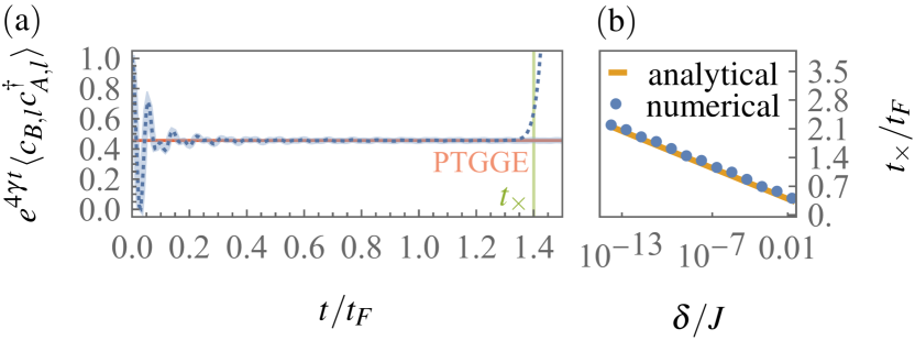
Figure 3: Relaxation of local correlations for a PT-symmetric quench with $\Delta J=-0.5J$, $\Delta\gamma=\gamma=0.2J$, and with small imbalance between loss and gain. (a) The dashed line corresponds to an imbalance of $\Delta=\delta/2=10^{-9}J$, while the solid line shows the evolution for balanced loss and gain, $\Delta=\delta=0$. For finite imbalance, the rescaled correlation function relaxes to the PTGGE prediction on intermediate time scales up to $t_{\times}$, indicated by a green vertical line. (b) The analytical prediction from Eq. (82) is in excellent agreement with the numerically determined values for a range of values of $\delta=2\Delta$. Numerically, we define $t_{\times}$ as the time at which the deviation from the PTGGE value equals one.

Finally, we want to contrast relaxation to the PTGGE with the asymptotic behavior of the covariance matrix in the PT-mixed and PT-breaking phases, again based on the dynamics of $\langle c_{B,l}c_{A,l}^{\dagger}(t)\rangle$, which, for $\delta=\Delta=0$, is given by

$$\langle c_{B,l}c_{A,l}^{\dagger}(t)\rangle=\int_{-\pi}^{\pi}\frac{dk}{4\pi}\,g_{1,k}^{2,1}(t).$$ (83)

In the PT-breaking phase, the dispersion is purely imaginary, $\omega_{k}=i\kappa_{k}$ with $\kappa_{k}\in\mathbb{R}_{>0}$ given in Eq. (34). After some algebraic simplifications of $g_{1,k}(t)$, the above integral reads [37]

$$\begin{split}\langle c_{B,l}c_{A,l}^{\dagger}(t)\rangle&=e^{-4\gamma t}\int_{-\pi}^{\pi}\frac{dk}{4\pi}\left(1-2\frac{h_{y,k}^{2}}{\kappa_{k}^{2}}\sinh(\kappa_{k}t)^{2}\right)\\ &\sim-e^{-4\gamma t}\int_{-\pi}^{\pi}\frac{dk}{8\pi}\frac{h_{y,k}^{2}}{\kappa_{k}^{2}}e^{2\kappa_{k}t}.\end{split}$$ (84)

Clearly, the dominant contribution is due to momenta in the vicinity of the maximum of $\kappa_{k}$. In the PT-mixed phase, the integration in Eq. (83) can be split into a contribution only consisting of PT-symmetric modes and another contribution due to PT-breaking modes, and again the dominant contribution at late times is due to PT-breaking modes in the vicinity of the maximum of $\kappa_{k}$. For example, for $\left\lvert\Delta J\right\rvert>J$, the dispersion $\kappa_{k}$ has a maximum at $k_{\mathrm{max}}=0$. Using standard asymptotic expansion techniques [90], we obtain

$$\langle c_{B,l}c_{A,l}^{\dagger}(t)\rangle\sim-e^{-4\gamma t}e^{4t\sqrt{\Delta\gamma^{2}-J^{2}}}t^{-3/2}.$$ (85)

That is, in the PT-mixed and PT-breaking phases, there is a single momentum mode $k_{\mathrm{max}}$ that maximizes $\kappa_{k}$ and dominates the dynamics, and the continuum of modes in the vicinity of $k_{\mathrm{max}}$ leads to additional algebraic decay. In contrast, all momenta $k\in\mathrm{BZ}$ contribute to the result for the PT-symmetric phase given in Eq. (75).

IV.1.2 Derivation of the PTGGE from the principle of maximum entropy

As we show next, the PTGGE can also be derived from the principle of maximum entropy [10] by properly taking into account the modified statistics of Liouvillian eigenmodes and the expectation values of their commutators. This approach is explained best by considering first the isolated SSH model. The dynamics of the isolated SSH model are generated by the Hamiltonian superoperator $\mathcal{H}$, whose action is defined in Eq. (2), and with eigenmodes $d_{s,k}$ given in Eq. (29). Since we are concerned with Gaussian states that are by definition fully determined by two-point functions, let us consider also quadratic forms of operators. Any quadratic form of eigenmodes $d_{s,k}$ can be expressed in terms of commutators and anticommutators through the decomposition

$$d_{s,k}d_{s^{\prime},k^{\prime}}^{\dagger}=\frac{1}{2}\left([d_{s,k},d_{s^{\prime},k^{\prime}}^{\dagger}]+\{d_{s,k},d_{s^{\prime},k^{\prime}}^{\dagger}\}\right).$$ (86)

For fermions, statistics are encoded in anticommutators,

$$\{d_{s,k},d_{s^{\prime},k^{\prime}}^{\dagger}\}=\delta_{s,s^{\prime}}\delta_{k,k^{\prime}},\quad\{d_{s,k},d_{s^{\prime},k^{\prime}}\}=\{d_{s,k}^{\dagger},d_{s^{\prime},k^{\prime}}^{\dagger}\}=0.$$ (87)

By contrast, commutators describe the dynamics. In particular, commutators of the modes $d_{s,k}$ are also eigenmodes of the Hamiltonian superoperator $\mathcal{H}$:

$$\begin{split}\mathcal{H}[d_{A,k},d_{A,k}^{\dagger}]&=0,\\ \mathcal{H}[d_{A,k},d_{B,k}^{\dagger}]&=-2\varepsilon_{k}[d_{A,k},d_{B,k}^{\dagger}].\end{split}$$ (88)

That is, mode-diagonal commutators are conserved, while mixed-index commutators oscillate with frequency $2\varepsilon_{k}$ and dephase. In quadratic fermionic models or in integrable models that can be mapped to noninteracting fermions, the GGE is usually stated as the maximum entropy ensemble that is compatible with conserved mode occupation numbers $n_{s,k}=d_{s,k}^{\dagger}d_{s,k}$ [16, 17]. According to our discussion, we can equivalently define the GGE as the maximum entropy ensemble that is consistent with canonical anticommutations relations Eq. (87) and the conservation of mode-diagonal commutators Eq. (88). Crucially, this latter definition generalizes to the PTGGE, however, with some important differences: First, the adjoint Liouvillian $\mathcal{L}^{\dagger}$ that generates the dynamics of operators in the driven-dissipative setting, and is specified below for the SSH model, is a non-Hermitian operator. Therefore, its eigenmodes obey modified noncanonical anticommutation relations. Second, mode-offdiagonal commutators of eigenmodes of $\mathcal{L}^{\dagger}$ oscillate at modified frequencies $2\omega_{k}$, directly affecting the dynamics. And third, mode-diagonal commutators are not conserved; instead, these commutators decay exponentially. But crucially, they do not oscillate and are, therefore, not affected by dephasing. Based on the above definition of the PTGGE, in the following, we present a detailed derivation of the PTGGE for the driven-dissipative SSH model. The computation consists of three steps: (i) Specifying the generator of operator dynamics $\mathcal{L}^{\dagger}$ and the corresponding eigenvalue equation. (ii) Solving the eigenvalue equation to obtain (ii.a) nonoscillatory, mode-diagonal and (ii.b) oscillatory, mode-offdiagonal commutators of eigenmodes of $\mathcal{L}^{\dagger}$. (iii) Constructing the PTGGE as the maximum entropy ensemble that is compatible with the statistics of the eigenmodes of the adjoint Liouvillian $\mathcal{L}^{\dagger}$ and the expectation values of nonoscillatory commutators.

(i) Adjoint Liouvillian.

As detailed in Appendix A, for a density matrix $\rho$ evolving according to a Liouvillian superoperator $\mathcal{L}$, the expectation value of an operator $O$ follows the equation of motion given by

$$\frac{d}{dt}\left\langle O\right\rangle=i\left\langle\mathcal{L}^{\dagger}O\right\rangle,$$ (89)

with the adjoint Liouvillian

$$\mathcal{L}^{\dagger}=\mathcal{H}-i\mathcal{D}^{\dagger}.$$ (90)

Hermitian conjugation is defined here with respect to the Hilbert-Schmidt scalar product, leading to $\mathcal{H}=\mathcal{H}^{\dagger}$, and

$$\begin{split}\mathcal{D}^{\dagger}O&=\sum_{l=1}^{L}\left(2L_{l}^{\dagger}OL_{l}-\{L_{l}^{\dagger}L_{l},O\}\right)\\ &=\sum_{l=1}^{L}\left([L_{l}^{\dagger},A]L_{l}+L_{l}^{\dagger}[A,L_{l}]\right).\end{split}$$ (91)

According to Eq. (89), the adjoint Liouvillian $\mathcal{L}^{\dagger}$ generates the dynamics of operator expectation values. Suppose now that $O$ is an eigenmode of $\mathcal{L}^{\dagger}$ in the following sense:

$$\mathcal{L}^{\dagger}O=\lambda^{*}\left(O-O_{\mathrm{SS}}\right),$$ (92)

where $O_{\mathrm{SS}}$ is a number. Then, the equation of motion of the expectation value $\langle O\rangle$ reduces to

$$\frac{d}{dt}\left\langle O\right\rangle=i\lambda^{*}\left(\left\langle O\right\rangle-O_{\mathrm{SS}}\right).$$ (93)

Dynamical stability requires the imaginary part of the eigenvalue $\lambda$ to be negative, such that the expectation value $\langle O\rangle$ approaches $O_{\mathrm{SS}}$ for $t\to\infty$.

(ii) Eigenmodes of the adjoint Liouvillian.

We want to solve the eigenvalue equation (92), where we consider quadratic eigenmodes of the adjoint Liouvillian. In particular, we seek eigenmodes in the form of mode-diagonal and mode-offdiagonal commutators,

$$\eta_{k}=[d_{s,k},d_{s,k}^{\dagger}],\qquad\chi_{k}=[d_{A,k},d_{B,k}^{\dagger}].$$ (94)

We note that only the commutators $\eta_{k}$ and $\chi_{k}$ and not the modes $d_{s,k}$ themselves satisfy the eigenvalue equation (92). Nevertheless, for simplicity, we refer to both the modes $d_{s,k}$ and the commutators $\eta_{k}$ and $\chi_{k}$ as eigenmodes of $\mathcal{L}^{\dagger}$. In analogy to Eq. (88), we anticipate that the expectation values of the diagonal commutators $\eta_{k}$ are nonoscillatory whereas the expectation values of the offdiagonal commutators $\chi_{k}$ are oscillatory and, therefore, subject to dephasing.

(ii.a) Nonoscillatory eigenmodes.

To find the nonoscillatory eigenmodes of the adjoint Liouvillian, we use a general bilinear ansatz given by

$$\eta=\sum_{l,l^{\prime}=1}^{2L}Q_{l,l^{\prime}}[c_{l},c_{l^{\prime}}^{\dagger}],$$ (95)

where the goal is to find $Q$ such that $\eta$ satisfies the eigenvalue equation (92). This approach does not rely on translational invariance and, therefore, we omit the momentum index for the time being. Plugging the ansatz into the eigenvalue equation (92), we obtain two contributions on the left-hand side that are due to the Hamiltonian superoperator $\mathcal{H}$ and the adjoint dissipator $\mathcal{D}^{\dagger}$, respectively. The Hamiltonian part reads

$$\mathcal{H}\eta=\sum_{l,l^{\prime}=1}^{2L}\left(c_{l}[Q,H]_{l,l^{\prime}}c_{l^{\prime}}^{\dagger}-c_{l^{\prime}}^{\dagger}[Q^{{\mathchoice{\raisebox{0.0pt}{$\displaystyle\intercal$}}{\raisebox{0.0pt}{$\textstyle\intercal$}}{\raisebox{0.0pt}{$\scriptstyle\intercal$}}{\raisebox{0.0pt}{$\scriptscriptstyle\intercal$}}}},H]_{l^{\prime},l}c_{l}\right),$$ (96)

and the action of the dissipator is given by

$$\mathcal{D}^{\dagger}\eta=-\sum_{l,l^{\prime}=1}^{2L}\left(c_{l}\{Q,M_{l}+M_{g}\}_{l,l^{\prime}}c_{l^{\prime}}^{\dagger}+c_{l^{\prime}}^{\dagger}\{M_{l}+M_{g},Q^{{\mathchoice{\raisebox{0.0pt}{$\displaystyle\intercal$}}{\raisebox{0.0pt}{$\textstyle\intercal$}}{\raisebox{0.0pt}{$\scriptstyle\intercal$}}{\raisebox{0.0pt}{$\scriptscriptstyle\intercal$}}}}\}_{l^{\prime},l}c_{l}\right)\\ +2\mathop{\mathrm{tr}}\!\left(\left(M_{l}-M_{g}\right)Q\right).$$ (97)

We write the eigenvalue $\lambda$ in Eq. (92) as $\lambda=-i\kappa$ with an undetermined real parameter $\kappa\in\mathbb{R}$, and we identify the steady-state value $\eta_{\mathrm{SS}}$ with the last term in Eq. (97),

$$\eta_{\mathrm{SS}}=\frac{2}{\kappa}\mathop{\mathrm{tr}}\!\left(\left(M_{l}-M_{g}\right)Q\right).$$ (98)

Then, the eigenvalue equation takes the form

$$\sum_{l,l^{\prime}=1}^{2L}\left[c_{l}\left(QZ^{\dagger}-ZQ\right)_{l,l^{\prime}}c_{l^{\prime}}^{\dagger}-c_{l^{\prime}}^{\dagger}\left(Z^{\dagger}Q^{{\mathchoice{\raisebox{0.0pt}{$\displaystyle\intercal$}}{\raisebox{0.0pt}{$\textstyle\intercal$}}{\raisebox{0.0pt}{$\scriptstyle\intercal$}}{\raisebox{0.0pt}{$\scriptscriptstyle\intercal$}}}}-Q^{{\mathchoice{\raisebox{0.0pt}{$\displaystyle\intercal$}}{\raisebox{0.0pt}{$\textstyle\intercal$}}{\raisebox{0.0pt}{$\scriptstyle\intercal$}}{\raisebox{0.0pt}{$\scriptscriptstyle\intercal$}}}}Z\right)_{l^{\prime},l}c_{l}\right]\\ =i\kappa\left(c_{l}Q_{l,l^{\prime}}c_{l^{\prime}}^{\dagger}-c_{l^{\prime}}^{\dagger}Q_{l^{\prime},l}^{{\mathchoice{\raisebox{0.0pt}{$\displaystyle\intercal$}}{\raisebox{0.0pt}{$\textstyle\intercal$}}{\raisebox{0.0pt}{$\scriptstyle\intercal$}}{\raisebox{0.0pt}{$\scriptscriptstyle\intercal$}}}}c_{l}\right).$$ (99)

Multiplying this equation with $c_{m}c_{m^{\prime}}^{\dagger}$ and using

$$\begin{split}\frac{1}{2^{2L}}\mathop{\mathrm{tr}}\!\left(c_{m}c_{m^{\prime}}^{\dagger}c_{l}c_{l^{\prime}}^{\dagger}\right)&=\frac{1}{4}\left(\delta_{m,m^{\prime}}\delta_{l,l^{\prime}}+\delta_{m,l^{\prime}}\delta_{l,m^{\prime}}\right),\\ \frac{1}{2^{2L}}\mathop{\mathrm{tr}}\!\left(c_{m}c_{m^{\prime}}^{\dagger}c_{l}^{\dagger}c_{l^{\prime}}\right)&=\frac{1}{4}\left(\delta_{m,m^{\prime}}\delta_{l,l^{\prime}}-\delta_{m,l}\delta_{m^{\prime},l^{\prime}}\right),\end{split}$$ (100)

we obtain two equations for $Q$ and its transpose $Q^{{\mathchoice{\raisebox{0.0pt}{$\displaystyle\intercal$}}{\raisebox{0.0pt}{$\textstyle\intercal$}}{\raisebox{0.0pt}{$\scriptstyle\intercal$}}{\raisebox{0.0pt}{$\scriptscriptstyle\intercal$}}}}$, respectively,

$$QZ^{\dagger}-ZQ =i\kappa Q$$ (101)

$$Z^{\dagger}Q^{{\mathchoice{\raisebox{0.0pt}{$\displaystyle\intercal$}}{\raisebox{0.0pt}{$\textstyle\intercal$}}{\raisebox{0.0pt}{$\scriptstyle\intercal$}}{\raisebox{0.0pt}{$\scriptscriptstyle\intercal$}}}}-Q^{{\mathchoice{\raisebox{0.0pt}{$\displaystyle\intercal$}}{\raisebox{0.0pt}{$\textstyle\intercal$}}{\raisebox{0.0pt}{$\scriptstyle\intercal$}}{\raisebox{0.0pt}{$\scriptscriptstyle\intercal$}}}}Z =i\kappa Q^{{\mathchoice{\raisebox{0.0pt}{$\displaystyle\intercal$}}{\raisebox{0.0pt}{$\textstyle\intercal$}}{\raisebox{0.0pt}{$\scriptstyle\intercal$}}{\raisebox{0.0pt}{$\scriptscriptstyle\intercal$}}}},$$ (102)

where $Z$ is defined in Eq. (14). Since $Z=Z^{{\mathchoice{\raisebox{0.0pt}{$\displaystyle\intercal$}}{\raisebox{0.0pt}{$\textstyle\intercal$}}{\raisebox{0.0pt}{$\scriptstyle\intercal$}}{\raisebox{0.0pt}{$\scriptscriptstyle\intercal$}}}}$, the two equations above are actually equivalent. To make further progress, we use translational invariance of the driven-dissipative SSH model, which implies that the eigenmodes $\eta_{k}$ are labeled by a momentum $k$, and that $Q_{k}$ are block Toeplitz matrices with $2\times 2$ blocks

$$q_{k,l-l^{\prime}}=\begin{pmatrix}Q_{k,2l-1,2l^{\prime}-1}&Q_{k,2l-1,2l^{\prime}}\\ Q_{k,2l,2l^{\prime}-1}&Q_{k,2l,2l^{\prime}}\end{pmatrix},$$ (103)

such that the commutator of Liouvillian eigenmodes in Eq. (94) now takes the form

$$\eta_{k}=\sum_{l,l^{\prime}=1}^{L}\left(C_{l}^{{\mathchoice{\raisebox{0.0pt}{$\displaystyle\intercal$}}{\raisebox{0.0pt}{$\textstyle\intercal$}}{\raisebox{0.0pt}{$\scriptstyle\intercal$}}{\raisebox{0.0pt}{$\scriptscriptstyle\intercal$}}}}q_{k,l-l^{\prime}}C_{l^{\prime}}^{\dagger{\mathchoice{\raisebox{0.0pt}{$\displaystyle\intercal$}}{\raisebox{0.0pt}{$\textstyle\intercal$}}{\raisebox{0.0pt}{$\scriptstyle\intercal$}}{\raisebox{0.0pt}{$\scriptscriptstyle\intercal$}}}}-C_{l^{\prime}}^{\dagger}q_{k,l-l^{\prime}}^{{\mathchoice{\raisebox{0.0pt}{$\displaystyle\intercal$}}{\raisebox{0.0pt}{$\textstyle\intercal$}}{\raisebox{0.0pt}{$\scriptstyle\intercal$}}{\raisebox{0.0pt}{$\scriptscriptstyle\intercal$}}}}C_{l}\right),$$ (104)

with $C_{l}=\left(c_{2l-1},c_{2l}\right)^{{\mathchoice{\raisebox{0.0pt}{$\displaystyle\intercal$}}{\raisebox{0.0pt}{$\textstyle\intercal$}}{\raisebox{0.0pt}{$\scriptstyle\intercal$}}{\raisebox{0.0pt}{$\scriptscriptstyle\intercal$}}}}$. Defining the discrete Fourier transformations of the blocks $q_{k,l}$ and the spinors $C_{l}$ as

$$q_{k,k^{\prime}}=\sum_{l=1}^{L}e^{-ik^{\prime}l}q_{k,l},\qquad C_{k}=\frac{1}{\sqrt{L}}\sum_{l=1}^{L}e^{-ikl}C_{l},$$ (105)

we can recast Eq. (102) as

$$z_{k^{\prime}}^{\dagger}q_{k,-k^{\prime}}^{{\mathchoice{\raisebox{0.0pt}{$\displaystyle\intercal$}}{\raisebox{0.0pt}{$\textstyle\intercal$}}{\raisebox{0.0pt}{$\scriptstyle\intercal$}}{\raisebox{0.0pt}{$\scriptscriptstyle\intercal$}}}}-q_{k,-k^{\prime}}^{{\mathchoice{\raisebox{0.0pt}{$\displaystyle\intercal$}}{\raisebox{0.0pt}{$\textstyle\intercal$}}{\raisebox{0.0pt}{$\scriptstyle\intercal$}}{\raisebox{0.0pt}{$\scriptscriptstyle\intercal$}}}}z_{k^{\prime}}=i\kappa q_{k,-k^{\prime}}^{{\mathchoice{\raisebox{0.0pt}{$\displaystyle\intercal$}}{\raisebox{0.0pt}{$\textstyle\intercal$}}{\raisebox{0.0pt}{$\scriptstyle\intercal$}}{\raisebox{0.0pt}{$\scriptscriptstyle\intercal$}}}},$$ (106)

and write the commutator in momentum space,

$$\eta_{k}=\sum_{k^{\prime}\in\mathrm{BZ}}\left(C_{k^{\prime}}^{{\mathchoice{\raisebox{0.0pt}{$\displaystyle\intercal$}}{\raisebox{0.0pt}{$\textstyle\intercal$}}{\raisebox{0.0pt}{$\scriptstyle\intercal$}}{\raisebox{0.0pt}{$\scriptscriptstyle\intercal$}}}}q_{k,-k^{\prime}}C_{k^{\prime}}^{\dagger{\mathchoice{\raisebox{0.0pt}{$\displaystyle\intercal$}}{\raisebox{0.0pt}{$\textstyle\intercal$}}{\raisebox{0.0pt}{$\scriptstyle\intercal$}}{\raisebox{0.0pt}{$\scriptscriptstyle\intercal$}}}}-C_{k^{\prime}}^{\dagger}q_{k,-k^{\prime}}^{{\mathchoice{\raisebox{0.0pt}{$\displaystyle\intercal$}}{\raisebox{0.0pt}{$\textstyle\intercal$}}{\raisebox{0.0pt}{$\scriptstyle\intercal$}}{\raisebox{0.0pt}{$\scriptscriptstyle\intercal$}}}}C_{k^{\prime}}\right).$$ (107)

In the PT-symmetric phase, $z_{k}$ can be diagonalized as stated in Eq. (220), and the spectrum of $z_{k}$ is given by $\sigma(z_{k})=\{-i2\gamma\pm\omega_{k}\}$ where $\omega_{k}\in\mathbb{R}_{>0}$. Using this representation of $z_{k}$ in Eq. (106), we obtain

$$\omega_{k^{\prime}}\left(U_{k^{\prime}}^{-\dagger}\sigma_{z}U_{k^{\prime}}^{\dagger}q_{k,-k^{\prime}}^{{\mathchoice{\raisebox{0.0pt}{$\displaystyle\intercal$}}{\raisebox{0.0pt}{$\textstyle\intercal$}}{\raisebox{0.0pt}{$\scriptstyle\intercal$}}{\raisebox{0.0pt}{$\scriptscriptstyle\intercal$}}}}-q_{k,-k^{\prime}}^{{\mathchoice{\raisebox{0.0pt}{$\displaystyle\intercal$}}{\raisebox{0.0pt}{$\textstyle\intercal$}}{\raisebox{0.0pt}{$\scriptstyle\intercal$}}{\raisebox{0.0pt}{$\scriptscriptstyle\intercal$}}}}U_{k^{\prime}}\sigma_{z}U_{k^{\prime}}^{-1}\right)=i\left(\kappa-4\gamma\right)q_{k,-k^{\prime}}^{{\mathchoice{\raisebox{0.0pt}{$\displaystyle\intercal$}}{\raisebox{0.0pt}{$\textstyle\intercal$}}{\raisebox{0.0pt}{$\scriptstyle\intercal$}}{\raisebox{0.0pt}{$\scriptscriptstyle\intercal$}}}},$$ (108)

with the shorthand notation $U_{k}^{-\dagger}=(U_{k}^{\dagger})^{-1}$. Then, identifying $\kappa=4\gamma$, we can rewrite this equation as a commutator,

$$\left[\sigma_{z},U_{k^{\prime}}^{\dagger}q_{k,-k^{\prime}}^{{\mathchoice{\raisebox{0.0pt}{$\displaystyle\intercal$}}{\raisebox{0.0pt}{$\textstyle\intercal$}}{\raisebox{0.0pt}{$\scriptstyle\intercal$}}{\raisebox{0.0pt}{$\scriptscriptstyle\intercal$}}}}U_{k^{\prime}}\right]=0.$$ (109)

Therefore, for $\eta_{k}$ to be an eigenmode of the adjoint Liouvillian with eigenvalue $\lambda=-i4\gamma$, $q_{k,k^{\prime}}$ has to satisfy the above commutation relation. The general solution for $q_{k,k^{\prime}}$ reads

$$q_{k,-k^{\prime}}^{{\mathchoice{\raisebox{0.0pt}{$\displaystyle\intercal$}}{\raisebox{0.0pt}{$\textstyle\intercal$}}{\raisebox{0.0pt}{$\scriptstyle\intercal$}}{\raisebox{0.0pt}{$\scriptscriptstyle\intercal$}}}}=U_{k^{\prime}}^{-\dagger}\left(\alpha_{\mathbbm{1},k,k^{\prime}}\mathbbm{1}+\alpha_{z,k,k^{\prime}}\sigma_{z}\right)U_{k^{\prime}}^{-1},$$ (110)

where $\alpha_{\mathbbm{1},k,k^{\prime}}$ and $\alpha_{z,k,k^{\prime}}$ are undetermined parameters. To obtain the solution anticipated in Eq. (94), we choose $\alpha_{\mathbbm{1},k,k^{\prime}}=\alpha_{z,k,k^{\prime}}=\alpha_{0,k}\delta_{k,k^{\prime}}/2$. Then, Eq. (107) takes the form

$$\eta_{k}=\frac{\alpha_{0,k}}{2}\left(C_{k}^{{\mathchoice{\raisebox{0.0pt}{$\displaystyle\intercal$}}{\raisebox{0.0pt}{$\textstyle\intercal$}}{\raisebox{0.0pt}{$\scriptstyle\intercal$}}{\raisebox{0.0pt}{$\scriptscriptstyle\intercal$}}}}U_{k}^{-{\mathchoice{\raisebox{0.0pt}{$\displaystyle\intercal$}}{\raisebox{0.0pt}{$\textstyle\intercal$}}{\raisebox{0.0pt}{$\scriptstyle\intercal$}}{\raisebox{0.0pt}{$\scriptscriptstyle\intercal$}}}}P_{z,+}U_{k}^{-\ast}C_{k}^{\dagger{\mathchoice{\raisebox{0.0pt}{$\displaystyle\intercal$}}{\raisebox{0.0pt}{$\textstyle\intercal$}}{\raisebox{0.0pt}{$\scriptstyle\intercal$}}{\raisebox{0.0pt}{$\scriptscriptstyle\intercal$}}}}-C_{k}^{\dagger}U_{k}^{-\dagger}P_{z,+}U_{k}^{-1}C_{k}\right),$$ (111)

where

$$P_{z,\pm}=\frac{1}{2}\left(\mathbbm{1}\pm\sigma_{z}\right).$$ (112)

Defining now the Liouvillian eigenmodes as

$$D_{k}=\begin{pmatrix}d_{A,k}\\ d_{B,k}\end{pmatrix}=V_{k}^{\dagger}C_{k}$$ (113)

with

$$V_{k}=\sqrt{\frac{2}{\mathop{\mathrm{tr}}\!\left(U_{k}^{-1}U_{k}^{-\dagger}\right)}}U_{k}^{-\dagger}=\frac{1}{\sqrt{2}}\begin{pmatrix}e^{-i\left(\phi_{k}+\psi_{k}\right)\!/2}&-e^{-i\left(\phi_{k}-\psi_{k}\right)\!/2}\\ e^{i\left(\phi_{k}+\psi_{k}\right)\!/2}&e^{i\left(\phi_{k}-\psi_{k}\right)\!/2}\end{pmatrix},$$ (114)

we obtain the final form of $\eta_{k}$:

$$\eta_{k}=[d_{A,k},d_{A,k}^{\dagger}].$$ (115)

The angle $\phi_{k}$ is defined in Eq. (218) and $\psi_{k}$ is determined by the relation

$$\varepsilon_{k}e^{i\psi_{k}}=\omega_{k}+i2\Delta\gamma.$$ (116)

In the transformation to the Liouvillian eigenmodes in Eq. (114), we have chosen the normalization such that $\{d_{A,k},d_{A,k}^{\dagger}\}=1$. This leads to

$$\alpha_{0,k}=\mathop{\mathrm{tr}}\!\left(U_{k}^{-1}U_{k}^{-\dagger}\right)=2\cosh(\theta_{k}),$$ (117)

with $\theta_{k}$ given in Eq. (219) and related to $\psi_{k}$ by

$$\tan(\psi_{k})=\sinh(\theta_{k}).$$ (118)

Note that the alternative choice $\alpha_{\mathbbm{1},k,k^{\prime}}=-\alpha_{z,k,k^{\prime}}=\alpha_{0,k}\delta_{k,k^{\prime}}/2$ in Eq. (110) leads to $\eta_{k}=[d_{B,k},d_{B,k}^{\dagger}]$. Further, the transformation $V_{k}$ given in Eq. (114) determines the statistics of the Liouvillian eigenmodes. Since $V_{k}$ is not unitary, the operators $d_{s,k}$ do not obey the usual canonical anticommutation relations. The statistics of these modes are encoded in the anticommutators collected in

$$\begin{pmatrix}\{d_{A,k},d_{A,k^{\prime}}\}&\{d_{A,k},d_{B,k^{\prime}}\}\\ \{d_{B,k},d_{A,k^{\prime}}\}&\{d_{B,k},d_{B,k^{\prime}}\}\end{pmatrix}=f_{k}\delta_{k,k^{\prime}},$$ (119)

where

$$f_{k}=V_{k}^{\dagger}V_{k}=\mathbbm{1}+\sin(\psi_{k})\sigma_{y}.$$ (120)

Next, having specified the solution for the matrix $Q$ that leads to eigenmodes $\eta_{k}$ in the form given in Eq. (115), we can determine the steady state contribution in Eq. (98). We find

$$\langle[d_{A,k},d_{A,k}^{\dagger}]\rangle_{\mathrm{SS}}=\eta_{\mathrm{SS}}=\frac{\delta}{\gamma}.$$ (121)

Finally, to fully determine the time evolution of the expectation value $\langle\eta_{k}\rangle$, we have to calculate its initial value. Relating the expectation value of the commutator to the covariance matrix by

$$\langle[d_{A,k},d_{A,k}^{\dagger}]\rangle=\frac{\omega_{k}}{\varepsilon_{k}}\mathop{\mathrm{tr}}\!\left(U_{k}^{-\dagger}P_{z,+}U_{k}^{-1}g_{k}\right),$$ (122)

we find the initial value, determined by the covariance matrix $g_{k}(0)$ in Eq. (51), to be given by

$$\langle[d_{A,k},d_{A,k}^{\dagger}]\rangle_{0}=\cos(\Delta\phi_{k}-\psi_{k}),$$ (123)

where the angle $\Delta\phi_{k}$ is defined in Eq. (74). Therefore, by solving Eq. (93) for the commutator in Eq. (115), we obtain the time evolution of the expectation value of diagonal commutators:

$$\langle[d_{A,k},d_{A,k}^{\dagger}](t)\rangle=e^{-4\gamma t}\langle[d_{A,k},d_{A,k}^{\dagger}]\rangle_{0}\\ +\left(1-e^{-4\gamma t}\right)\langle[d_{A,k},d_{A,k}^{\dagger}]\rangle_{\mathrm{SS}},$$ (124)

with the initial and steady-state values given in Eq. (123) and Eq. (121), respectively.

(ii.b) Oscillatory eigenmodes.

We proceed by showing that the offdiagonal commutators $\chi_{k}=[d_{A,k},d_{B,k}^{\dagger}]$ with mode operators $d_{s,k}$ given in Eq. (113) are oscillatory eigenmodes of the Liouvillian. To that end we write $\chi_{k}$ in the form

$$\chi_{k}=\sum_{k^{\prime}\in\mathrm{BZ}}\left(C_{k^{\prime}}^{{\mathchoice{\raisebox{0.0pt}{$\displaystyle\intercal$}}{\raisebox{0.0pt}{$\textstyle\intercal$}}{\raisebox{0.0pt}{$\scriptstyle\intercal$}}{\raisebox{0.0pt}{$\scriptscriptstyle\intercal$}}}}p_{k,k^{\prime}}^{{\mathchoice{\raisebox{0.0pt}{$\displaystyle\intercal$}}{\raisebox{0.0pt}{$\textstyle\intercal$}}{\raisebox{0.0pt}{$\scriptstyle\intercal$}}{\raisebox{0.0pt}{$\scriptscriptstyle\intercal$}}}}C_{k^{\prime}}^{\dagger{\mathchoice{\raisebox{0.0pt}{$\displaystyle\intercal$}}{\raisebox{0.0pt}{$\textstyle\intercal$}}{\raisebox{0.0pt}{$\scriptstyle\intercal$}}{\raisebox{0.0pt}{$\scriptscriptstyle\intercal$}}}}-C_{k^{\prime}}^{\dagger}p_{k,k^{\prime}}C_{k}\right),$$ (125)

where we define

$$p_{k,k^{\prime}}=\delta_{k,k^{\prime}}V_{k^{\prime}}\sigma_{-}V_{k^{\prime}}^{\dagger},$$ (126)

and $\sigma_{\pm}=(\sigma_{x}\pm i\sigma_{y})/2$. The fact that the offdiagonal commutators $\chi_{k}$ are eigenmodes of $\mathcal{L}^{\dagger}$ with eigenvalue $\lambda=-2\left(\omega_{k}+i2\gamma\right)$ can be confirmed by noting that $p_{k,k^{\prime}}$ satisfies the eigenvalue equation that is similar to Eq. (106):

$$z_{k^{\prime}}^{\dagger}p_{k,k^{\prime}}-p_{k,k^{\prime}}z_{k^{\prime}}=-\left(2\omega_{k}-i4\gamma\right)p_{k,k^{\prime}}.$$ (127)

The time evolution of expectation values of $\chi_{k}$ thus reads

$$\langle[d_{A,k},d_{B,k}^{\dagger}](t)\rangle=e^{-i2\left(\omega_{k}-i2\gamma\right)t}\langle[d_{A,k},d_{B,k}^{\dagger}]\rangle_{0}\\ +\left(1-e^{-i2(\omega_{k}-i2\gamma)t}\right)\langle[d_{A,k},d_{B,k}^{\dagger}]\rangle_{\mathrm{SS}},$$ (128)

where the initial and steady-state values are given by

$$\begin{split}\langle[d_{A,k},d_{B,k}^{\dagger}]\rangle_{0}&=i\sin(\Delta\phi_{k}),\\ \langle[d_{A,k},d_{B,k}^{\dagger}]\rangle_{\mathrm{SS}}&=\frac{i\Delta\cos(\psi_{k})-\delta\sin(\psi_{k})}{2\left(\omega_{k}-2i\gamma\right)}.\end{split}$$ (129)

(iii) Construction of the PTGGE.

We consider now the case of balanced loss and gain with $\delta=\Delta=0$, such that the steady state contributions to Eqs. (124) and (128) vanish,

$$\langle[d_{A,k},d_{A,k}^{\dagger}]\rangle_{\mathrm{SS}}=\langle[d_{A,k},d_{B,k}^{\dagger}]\rangle_{\mathrm{SS}}=0.$$ (130)

Further, due to the oscillatory exponent in (128), the contribution of offdiagonal commutators to local observables vanishes at late times due to dephasing between offdiagonal commutators with different momenta

$$\langle[d_{A,k},d_{B,k}^{\dagger}](t)\rangle\to 0.$$ (131)

Therefore, the state of the system at late times is determined by the expectation values of diagonal commutators given in Eq. (124) and the statistics of the modes $d_{s,k}$ that follow from the nonunitary transformation $V_{k}$ Eq. (114) and are encoded in the matrix $f_{k}$ in Eq. (120). The PTGGE can be defined as the maximum entropy ensemble that is compatible with these requirements. We can also collect the same information in the dephased covariance given in Eq. (76), which can be related to the eigenmodes by

$$g_{\mathrm{PTGGE},k}(t)=V_{k}^{-\dagger}\zeta_{k}(t)V_{k}^{-1}.$$ (132)

where $\zeta_{k}(t)=e^{-4\gamma t}\zeta_{k}^{\prime}$ with

$$\begin{split}\zeta_{k}^{\prime}&=\begin{pmatrix}\langle[d_{A,k},d_{A,k}^{\dagger}]\rangle_{0}&0\\ 0&\langle[d_{B,k},d_{B,k}^{\dagger}]\rangle_{0}\end{pmatrix}\\ &=\begin{pmatrix}\cos(\Delta\phi_{k}-\psi_{k})&0\\ 0&-\cos(\Delta\phi_{k}+\psi_{k})\end{pmatrix}.\end{split}$$ (133)

Then for the given two-point function $g_{\mathrm{PTGGE},k}(t)$, the entropy is maximized for the Gaussian state that is uniquely determined through Eq. (77). In terms of the eigenmodes of the adjoint Liouvillian, the PTGGE can be written as

$$\rho_{\mathrm{PTGGE}}(t)=\frac{1}{Z_{\mathrm{PTGGE}}(t)}e^{-2\sum_{k\in\mathrm{BZ}}D_{k}^{\dagger}f_{k}^{-1}\mathrm{arctanh}\left(\zeta_{k}(t)f_{k}^{-1}\right)D_{k}},$$ (134)

which shows most transparently both the dependence of the PTGGE on the initial conditions through $\zeta_{k}(t)$ and the effect of the noncanonical anticommutation relations of the Liouvillian eigenmodes described by $f_{k}$.

IV.2 Driven-dissipative Kitaev chain

Having presented the derivation of the PTGGE for the SSH model, we now turn to the driven-dissipative Kitaev chain. Since the latter has been discussed in detail in Ref. [37], we restrict ourselves here to highlighting the aspects in which the derivation for the Kitaev chain differs from the one for the SSH model. In particular, for the Kitaev chain, we define bilinear forms of eigenmodes as

$$\eta_{k}=[d_{k},d_{k}^{\dagger}],\qquad\chi_{k}=[d_{k},d_{-k}],$$ (135)

which can be regarded as normal and anomalous commutators, respectively, and where the Liouvillian eigenmodes $d_{k}$ are related to the original fermionic operators $c_{k}=\frac{1}{\sqrt{L}}\sum_{l=1}^{L}e^{-ikl}c_{l}$ via

$$D_{k}=\begin{pmatrix}d_{k}\\ d_{-k}^{\dagger}\end{pmatrix}=V_{k}^{\dagger}\begin{pmatrix}c_{k}\\ c_{-k}^{\dagger}\end{pmatrix},\quad V_{k}=\begin{pmatrix}\cos\!\left(\frac{\theta_{k}+\phi_{k}}{2}\right)&i\sin\!\left(\frac{\theta_{k}-\phi_{k}}{2}\right)\\ i\sin\!\left(\frac{\theta_{k}+\phi_{k}}{2}\right)&\cos\!\left(\frac{\theta_{k}-\phi_{k}}{2}\right)\end{pmatrix},$$ (136)

with angles $\theta_{k}$ and $\phi_{k}$ that are defined through the relations

$$\begin{split}\varepsilon_{k}e^{i\theta_{k}}&=-2J\cos(k)-\mu+i2\Delta\sin(k),\\ \varepsilon_{k}e^{i\phi_{k}}&=\omega_{k}+i2\sqrt{\gamma_{l}\gamma_{g}}.\end{split}$$ (137)

The Liouvillian eigenmodes $d_{k}$ obey noncanonical anticommutation relations,

$$\begin{pmatrix}\{d_{k},d_{k^{\prime}}^{\dagger}\}&\{d_{k},d_{-k^{\prime}}\}\\ \{d_{-k}^{\dagger},d_{k^{\prime}}^{\dagger}\}&\{d_{-k}^{\dagger},d_{-k^{\prime}}\}\end{pmatrix}=f_{k}\delta_{k,k^{\prime}},$$ (138)

where $f_{k}=V_{k}^{\dagger}V_{k}=\mathbbm{1}+\sin(\phi_{k})\sigma_{y}$. In analogy to the mode-diagonal commutators for the SSH model, the normal commutators $\eta_{k}$ are nonoscillatory,

$$\langle[d_{k},d_{k}^{\dagger}](t)\rangle=e^{-4\gamma t}\langle[d_{k},d_{k}^{\dagger}]\rangle_{0}+\left(1-e^{-4\gamma t}\right)\langle[d_{k},d_{k}^{\dagger}]\rangle_{\mathrm{SS}},$$ (139)

where $\langle[d_{k},d_{k}^{\dagger}]\rangle_{0}$ is determined by the initial conditions and $\langle[d_{k},d_{k}^{\dagger}]\rangle_{\mathrm{SS}}$ contains the steady state contribution. The nonoscillatory normal commutators decay with an overall decay rate $\gamma$ defined in Eq. (62), and are not affected by dephasing. In contrast, and analogously to the mode-offdiagonal commutators of the SSH model, the anomalous commutators $\chi_{k}$ are oscillatory,

$$\langle[d_{k},d_{-k}](t)\rangle=e^{-i2\left(\omega_{k}-i2\gamma\right)t}\langle[d_{k},d_{-k}]\rangle_{0}\\ +\left(1-e^{-i2(\omega_{k}-i2\gamma)t}\right)\langle[d_{k},d_{-k}]\rangle_{\mathrm{SS}},$$ (140)

with initial values $\langle[d_{k},d_{-k}]\rangle_{0}$ and steady-state contributions $\langle[d_{k},d_{-k}]\rangle_{\mathrm{SS}}$. The anomalous commutators oscillate with frequency $\omega_{k}$ and are thus affected by dephasing. As above, the PTGGE describes the late-time relaxation dynamics for vanishing steady-state contributions $\langle[d_{k},d_{k}^{\dagger}]\rangle_{\mathrm{SS}}=\langle[d_{k},d_{-k}]\rangle_{\mathrm{SS}}=0$, accomplished by balanced loss and gain rates $\delta=\gamma_{l}-\gamma_{g}=0$, and after dephasing of the contributions due to anomalous commutators. The explicit form of the PTGGE is given by

$$\rho_{\mathrm{PTGGE}}(t)=\frac{1}{Z_{\mathrm{PTGGE}}(t)}e^{-2\sum_{k\geq 0}D_{k}^{\dagger}f_{k}^{-1}\mathrm{arctanh}\left(\zeta_{k}(t)f_{k}^{-1}\right)D_{k}},$$ (141)

where $\zeta_{k}(t)=e^{-4\gamma t}\zeta_{k}^{\prime}$ with

$$\zeta_{k}^{\prime}=\begin{pmatrix}\langle[d_{k},d_{k}^{\dagger}]\rangle_{0}&0\\ 0&\langle[d_{-k}^{\dagger},d_{-k}]\rangle_{0}\end{pmatrix}.$$ (142)

The key difference between Eqs. (141) and (134) for the Kitaev chain and the SSH model, respectively, is that in general anomalous correlations such as $\langle c_{l}c_{l^{\prime}}\rangle$ do not vanish for the Kitaev chain; in contrast, the weak $\mathrm{U}(1)$ symmetry of the driven-dissipative SSH model ensures that anomalous correlations like $\langle c_{s,l}c_{s^{\prime},l^{\prime}}\rangle$ vanish at all times.

V Spreading of correlations

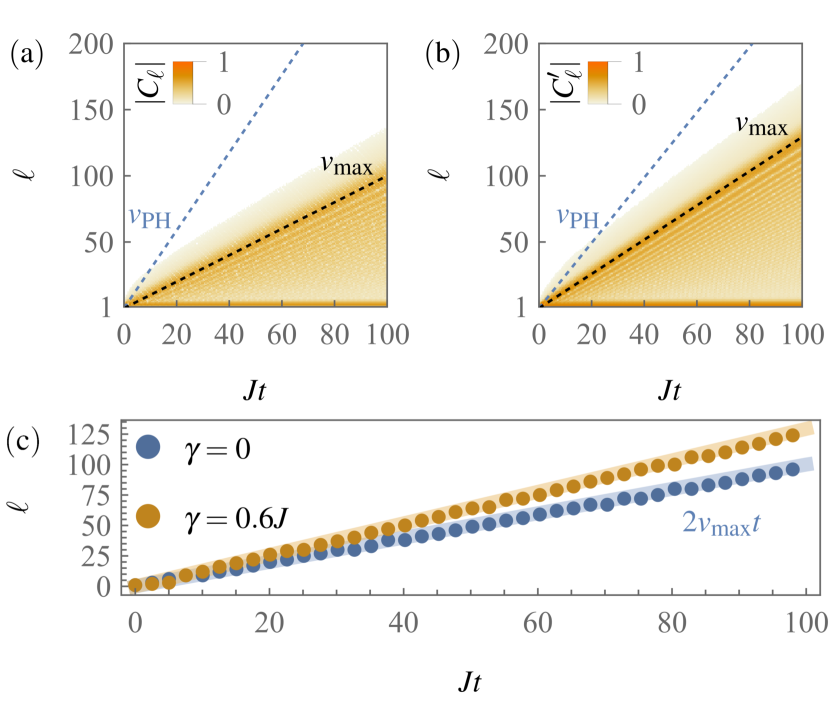
Figure 4: Propagation of correlations after quenches to the topological PT-symmetric phase ($\mu=-0.5J$) for (a) the isolated system ($\gamma=0$) and (b) the driven dissipative system ($\gamma=0.6J$). The black and blue dashed lines are described by $\ell=2v_{\mathrm{max}}t$ and $\ell=2v_{\mathrm{PH}}t$, respectively. (c) Direct comparison between the numerically determined peak positions (dots) and $\ell=2v_{\mathrm{max}}t$ (solid lines).

Now that we have derived the ensemble that describes the late-time dynamics for quenches to the PT-symmetric phase, we turn to a detailed study of relaxation to the PTGGE. In the following sections, both for the SSH model and the Kitaev chain, we focus on balanced loss and gain with $\delta=\Delta=0$, such that the steady state is at infinite temperature, and a description of the dynamics in terms of a PTGGE applies on arbitrarily long time scales.

A well-established property of isolated integrable systems that exhibit generalized thermalization after a quantum quench is the ballistic propagation of correlations through the system [16, 18]. This is also referred to as light cone spreading of correlations, since correlations outside of the light cone that is defined by the group velocity $v_{\mathrm{max}}$ are suppressed exponentially [91]. As we demonstrate in the following, light cone propagation of correlations is not unique to isolated systems [92, 93]. We illustrate this behavior for the driven-dissipative Kitaev chain, where we consider the evolution of the normal commutators $C_{l-l^{\prime}}(t)=\langle[c_{l},c_{l^{\prime}}^{\dagger}](t)\rangle$ for $\delta=\Delta=0$. In the PT-symmetric phase, we find ballistic propagation of quasiparticles which, however, have a finite lifetime, and a maximum velocity adjusted to the modified dispersion relation $\omega_{k}$; in contrast, in the PT-mixed and PT-broken phases, we observe diffusive spreading of correlations.

V.1 PT-symmetric phase

In Figs. 4(a) and (b), we show the absolute value of rescaled normal commutators $C^{\prime}_{\ell}(t)=e^{4\gamma t}C_{\ell}(t)$ for the isolated and the driven-dissipative Kitaev chain in the PT-symmetric phase, respectively. A clear light cone structure is visible in both figures. The peak of correlations, defining the boundary of the light cone and found at position $\ell=2v_{\mathrm{max}}t$, is well described by the ballistic propagation of quasiparticles with finite lifetime $\sim 1/\gamma$ and velocity

$$v_{\mathrm{max}}=\max_{k\in\mathrm{BZ}}\!\left(\left\lvert v_{k}\right\rvert\right)=\max_{k\in\mathrm{BZ}}\!\left(\left\lvert d\omega_{k}/dk\right\rvert\right).$$ (143)

We conclude that the spreading of correlations with finite velocity is maintained also in the driven-dissipative model throughout the whole PT-symmetric phase. For a finite rate of dissipation $\gamma$, the light cone velocity with dispersion $\omega_{k}$ is increased compared to the velocity corresponding to the isolated system with dispersion $\varepsilon_{k}$. This is further verified in Fig. 4(c), where the position of the light cone boundary is traced numerically and compared to the analytical prediction. However, the increased speed at which correlations propagate is offset by the exponential decay of correlations at rate $4\gamma$. Further, the phase velocity defined as [94]

$$v_{\mathrm{PH}}=\left\lvert\omega_{k}/k\right\rvert_{k=k_{\mathrm{max}}},$$ (144)

where $k_{\mathrm{max}}$ is the momentum for which $v_{k}=v_{\mathrm{max}}$, decreases with increasing reservoir coupling. While $v_{\mathrm{max}}$ defines the boundary beyond which correlators become exponentially suppressed, the phase velocity describes the propagation of local peaks within the light cone. At the boundaries of the PT-symmetric phase, the phase velocity and maximum particle velocity line up with $v_{\mathrm{max}}=v_{\mathrm{PH}}=\sqrt{2J\left\lvert\mu\right\rvert}$ for $\mu<0$, while for $\mu>0$ we still have $v_{\mathrm{max}}=\sqrt{2J\left\lvert\mu\right\rvert}$ but the phase velocity $v_{\mathrm{PH}}=0$. This behavior is depicted in Fig. 5, where $v_{\mathrm{max}}$ and $v_{\mathrm{PH}}$ are plotted as a function of $\mu$.

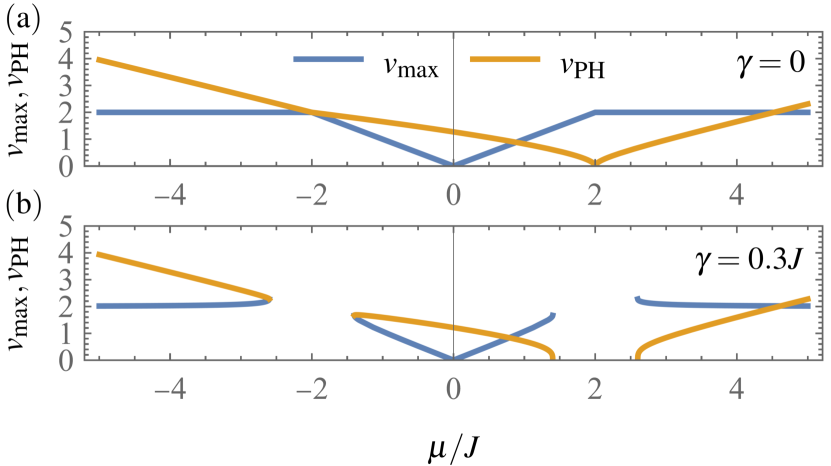
Figure 5: Maximum of the quasiparticle velocity $v_{\mathrm{max}}$ and the phase velocity $v_{\mathrm{PH}}$ as a function of the chemical potential $\mu$ for (a) the isolated system ($\gamma=0$) and (b) the driven-dissipative system ($\gamma=0.3J$). For $\mu<0$, at the phase boundary, $v_{\mathrm{max}}=v_{\mathrm{PH}}=\sqrt{2J\left\lvert\mu\right\rvert}$, while for $\mu>0$, we find $v_{\mathrm{max}}=\sqrt{2J\left\lvert\mu\right\rvert}$ and $v_{\mathrm{PH}}=0$.

V.2 PT-mixed and PT-broken phases

In the PT-mixed and PT-broken phases, where $\gamma>\gamma_{c}=\left|J-\left\lvert\mu\right\rvert/2\right|$, the spreading of correlations is dominated by the single slowest-decaying mode with decay rate

$$2\gamma_{s}=\min_{k\in\mathrm{BZ}}\!\left(-\mathop{\mathrm{Im}}(\lambda_{+,k})\right).$$ (145)

Accordingly, we define rescaled normal commutators as $C_{l}^{\prime}(t)=e^{4\gamma_{s}t}C_{l}(t)$. In Fig. 6(a) and (b), the absolute value of rescaled normal commutators is shown for the PT-mixed and PT-broken phase, respectively. It is worthwhile to first discuss the qualitative differences of correlations in the phases with PT-symmetric and PT-breaking modes. In the PT-symmetric phase, at any time, the normal commutators show multiple oscillations inside the light cone, with a peak at the boundary of the light cone and ensuing suppression of correlations outside the light cone. This creates the sharp boundaries in Fig. 4. In contrast, in the presence of PT-breaking modes, normal commutators show a single peak without oscillations and long decaying tails, giving the unstructured appearance inside the boundary in Fig. 6. Crucially, a correlation boundary can still be defined through this single peak. The correlation boundary, however, spreads diffusively according to $\ell=2(Dt)^{1/2}$, where the diffusion constant is given by

$$D=\left.-\frac{1}{2}\frac{d^{2}\kappa_{k}}{dk^{2}}\right\rvert_{k=k_{\mathrm{max}}}=\frac{J\left\lvert\mu\right\rvert}{\sqrt{4\gamma_{l}\gamma_{g}-\left(2J-\left\lvert\mu\right\rvert\right)^{2}}},$$ (146)

with $\kappa_{k}$ defined in Eq. (34) and $k_{\mathrm{max}}$ the momentum maximizing $\kappa_{k}$. The diffusive evolution of the peak position is illustrated further in Fig. 6(c).

Figure 6: Propagation of correlations after quenches to (a) the PT-mixed phase ($\mu=-0.5$, $\gamma=1J$) and (b) the PT-broken phase ($\mu=-0.5$, $\gamma=2J$). The red dots indicate the position of the peak of correlations, spreading diffusively as $\ell=2\left(Dt\right)^{1/2}$. (c) Direct comparison between the numerically determined peak positions (dots) and diffusive propagation in log-log scale.

Let us briefly comment on the spreading of correlations in the driven-dissipative SSH model. Based on the analytical form of the covariance matrix derived in Sec. III.1.4, which is structurally similar to the covariance matrix of the Kitaev chain, we can expect that the dynamics of correlations is qualitatively the same in both models. This expectation is confirmed by numerical results, which we do not show here.

VI Time evolution of the subsystem entropy

The linear growth and volume-law saturation of the von Neumann entropy of a finite subsystem is a key signature of thermalization in isolated systems[19, 20, 21, 22]. As we show in the following, the exact same phenomenology can be observed after quenches to the PT-symmetric phase of the driven-dissipative SSH model—if we consider the contribution to the entropy that measures the spreading of correlations due to the propagation of pairs of entangled quasiparticles, and after appropriate rescaling to compensate for exponential decay. The corresponding analysis for the driven-dissipative Kitaev chain is provided in Ref. [37].

We consider a subsystem of the SSH chain that contains $\ell$ contiguous unit cells. The corresponding reduced density matrix is obtained by tracing out the remaining $L-\ell$ unit cells, $\rho_{\ell}=\mathop{\mathrm{tr}}_{L-\ell}(\rho)$, and the von Neumann subsystem entropy is defined by $S_{\mathrm{vN},\ell}=-\mathop{\mathrm{tr}}(\rho_{\ell}\ln(\rho_{\ell}))$. For a Gaussian state, the subsystem entropy can be calculated as [89]

$$S_{\mathrm{vN},\ell}=\sum_{l=1}^{\ell}S(\xi_{l}),$$ (147)

where

$$S(\xi)=-\frac{1+\xi}{2}\ln\left(\frac{1+\xi}{2}\right)-\frac{1-\xi}{2}\ln\left(\frac{1-\xi}{2}\right),$$ (148)

and where $\pm\xi_{l}$ with $0\leq\xi_{l}\leq 1$ and $l\in\{1,\dots,\ell\}$ are the eigenvalues of the reduced covariance matrix $G_{\ell}$ defined by

$$G_{\ell}=\left(G^{s,s^{\prime}}_{l,l^{\prime}}\right)^{s,s^{\prime}\in\{A,B\}}_{l,l^{\prime}\in\{1,\dotsc,\ell\}},$$ (149)

with $G^{s,s^{\prime}}_{l,l^{\prime}}$ given in Eq. (6). The set of eigenvalues $\{\pm\xi_{l}\}$ of $G_{\ell}$ forms the single-particle entanglement spectrum [89]. In pure states of isolated systems, the subsystem entropy measures the entanglement between the subsystem and its compliment. After a quench, the subsystem entropy grows linearly in $t$ before it saturates to a volume-law value, $S_{\mathrm{vN},\ell}\propto\ell$. This behavior can be explained through a quasiparticle picture, which does not only provide a qualitative interpretation but also quantitative predictions for the full time evolution after a quench in the space-time scaling limit [19, 20, 21, 22]. In this picture, the initial state acts as a source of pairs of entangled quasiparticles with opposite momenta. After creation, these quasiparticles move ballistically with a velocity of at most $v_{\mathrm{max}}$ through the system. All pairs whose members are separated by the boundary between the subsystem and its compliment contribute to the subsystem entropy. Consequently, the subsystem entropy starts to saturate when all maximum-velocity pairs generated in the subsystem have left the subsystem.

In open systems, the time-evolved state is no longer pure and the subsystem entropy involves two contributions [95, 40, 39, 38]: $S_{\mathrm{vN},\ell}^{\mathrm{QP}}$, which describes correlations due to quasiparticle pairs as in an isolated system; and $S_{\mathrm{vN}}^{\mathrm{stat}}=S_{\mathrm{vN},L}$, the statistical entropy due to the mixedness of the state. The quasiparticle-pair contribution is thus given by the difference

$$S_{\mathrm{vN},\ell}^{\mathrm{QP}}=S_{\mathrm{vN},\ell}-\frac{\ell}{L}S_{\mathrm{vN}}^{\mathrm{stat}}.$$ (150)

In the following, we consider quenches to the PT-symmetric phase of the driven-dissipative SSH model. Building upon findings of Refs. [39, 38], in Ref. [37], we have proposed an analytical conjecture for the evolution of the quasiparticle-pair contribution $S_{\mathrm{vN},\ell}^{\mathrm{QP}}$ in the space-time scaling limit:

$$S_{\mathrm{vN},\ell}^{\mathrm{QP}}(t)\sim\int_{0}^{\pi}\min(2\left\lvert v_{k}\right\rvert t,\ell)\mathop{\mathrm{tr}}\left(S\!\left(\zeta_{k}(t)f_{k}^{-1}\right)-S(g_{k}(t))_{d}\right),$$ (151)

where for the SSH model $\zeta_{k}(t)$ and $f_{k}$ are defined in Eqs. (133) and (120), respectively, and $g_{k}(t)$ is given in Eq. (48) with the subscript “d,” which stands for dephasing, indicating that only nonoscillatory components contribute. For long times, $\gamma t\gg 1$, we can expand the quasiparticle-pair entropy in the exponentially decaying factors $\zeta_{k}(t),g_{k}(t)\sim e^{-4\gamma t}$. To lowest nontrivial order, we find $S(\xi)\sim\ln(2)-\xi^{2}/2$. Then, the constant contributions in Eq. (151) cancel, and we find $S_{\mathrm{vN},\ell}^{\mathrm{QP}}(t)\sim e^{-8\gamma t}$. Therefore, relaxation to the PTGGE can be revealed by considering the rescaled quasiparticle-pair entropy $e^{8\gamma t}S_{\mathrm{vN},\ell}^{\mathrm{QP}}(t)$, which is shown in Fig. 7. The rescaled quasiparticle-pair entropy grows linearly up to the Fermi time [14],

$$t_{F}=\ell/(2v_{\mathrm{max}}),$$ (152)

where saturation to the value predicted by the PTGGE sets in. As shown in the inset, the difference between the numerical results and the analytical conjecture Eq. (150) vanishes as $1/\ell$. The numerical method we have used to obtain this data is described in Ref. [37].

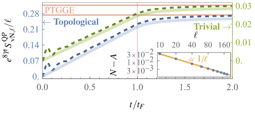
Figure 7: Quasiparticle-pair contribution to the subsystem entropy in the driven-dissipative SSH model after quenches to the trivial (green, $\Delta J=0.5J$) and topological (blue, $\Delta J=-0.5J$) PT-symmetric phases for $\gamma=\Delta\gamma=0.1J$, $\delta=\Delta=0$, and $\ell=20$. Dashed lines show numerical data, and solid lines correspond to the analytical conjecture Eq. (151) for the space-time scaling limit. The approach of the numerical results to the conjecture with increasing subsystem size is shown in the inset: For the topological quench at $t=2t_{F}$, the difference between the numerical data and Eq. (151) (blue dots) vanishes as $1/\ell$ (orange line).

VII Time evolution of string order and subsystem fermion parity

Generalized thermalization after a quantum quench in isolated systems is defined as relaxation of the averages of local observables to stationary values that are determined by the GGE. Similarly, based on the arguments given in Sec. IV, after quenches to the PT-symmetric phases of the driven-dissipative Kitaev and SSH chains, we expect to observe local relaxation to the PTGGE. To confirm this expectation, we proceed to study the time evolution of the dual string order parameter for the SSH model and the subsystem parity for the Kitaev chain, which are defined below in Secs. VII.1 and VII.2, respectively. These observables are of special interest due to their connection to topology: On the one hand, in the ground state of an isolated system, the dual string order parameter and the subsystem parity function as topological disorder parameters. That is, they are finite in the trivial phase and vanish in the topological phase. On the other hand, after quenches originating from the trivial phase, the decay of dual string order and subsystem parity carries a robust signature of the topology of the postquench Hamiltonian: For quenches across the topological phase boundary, the topological disorder parameters exhibit periodically recurring zero crossings; in contrast, they do not cross zero for quenches within the trivial phase. Physically, these zero crossings correspond to pumping of spin order and fermion parity between a finite subsystem and its complement. As we discuss in the following, in the presence of drive and dissipation, this phenomenology acquires qualitative modifications that are unique to open systems.

VII.1 Dual string order parameter

The concept of string order has originally been introduced and is mostly discussed in the context of spin chains [96, 97]. For the SSH model Eq. (4), an equivalent formulation in terms of a dimerized spin-$\nicefrac{{1}}{{2}}$ chain can be obtained through the Jordan-Wigner transformation [98], which yields

$$H=2\sum_{l=1}^{2L}\left(J-\left(-1\right)^{l}\Delta J\right)\left(S^{x}_{l}S^{x}_{l+1}+S^{y}_{l}S^{y}_{l+1}\right),$$ (153)

where $S_{l}^{\mu}$ with $\mu\in\{x,y,z\}$ are spin-$\nicefrac{{1}}{{2}}$ operators that act on the spin at site $l$ with $l\in\{1,\dotsc,2L\}$. The Jordan-Wigner transformation, which maps the set of $2L$ fermionic operators $c_{l}$ and $c_{l}^{\dagger}$ with $c_{A,l}=c_{2l-1}$ and $c_{B,l}=c_{2l}$ to spin operators $S_{l}^{\pm}=S_{l}^{x}\pm iS_{l}^{y}$, is given by

$$S_{l}^{-}=e^{i\pi\sum_{l^{\prime}=1}^{l-1}n_{l^{\prime}}}c_{l},\quad S_{l}^{+}=e^{i\pi\sum_{l^{\prime}=1}^{l-1}n_{l^{\prime}}}c_{l}^{\dagger},\quad S_{l}^{z}=n_{l}-\frac{1}{2}.$$ (154)

where $n_{l}=c_{l}^{\dagger}c_{l}$. For $\Delta J<0$, the ground state of the dimerized spin chain is topologically ordered. Indeed, the topologically ordered phase of the dimerized spin-$\nicefrac{{1}}{{2}}$ chain is continuously connected to the Haldane phase of the antiferromagnetic spin-1 Heisenberg chain [99]. The topological and trivial phases of the dimerized spin chain can be distinguished through the string order parameter, which takes a finite expectation value in the topological phase, and vanishes in the trivial phase. Equivalently, the dual string order parameter is nonzero in the trivial phase, and vanishes in the topological phase [73]. The designation as dual refers here to the self duality of the dimerized spin chain: Under a translation by one lattice site, $S_{l}^{\mu}\mapsto S_{l+1}^{\mu}$, the Hamiltonian Eq. (153) maps to itself with $\Delta J\mapsto-\Delta J$. Consequently, also the trivial and topological phases are exchanged, and, therefore, the dual string order parameter, which is obtained by performing the translation by one lattice site on the usual string order parameter, serves as a topological disorder parameter. The dual string order parameter for the dimerized spin-$\nicefrac{{1}}{{2}}$ chain is given by [73, 100]

$$O_{\ell}^{\mu}=e^{i\pi\sum_{l=1}^{2\ell}S_{l}^{\mu}},$$ (155)

with $\mu\in\{x,y\}$. We note that the invariance of the Hamiltonian Eq. (153) under rotations around the $z$-axis implies that $\langle O_{\ell}^{x}\rangle=\langle O_{\ell}^{y}\rangle$. An alternative interpretation of string order is obtained through a nonlocal unitary transformation that maps the dimerized spin chain Eq. (153) to two coupled Ising models [101], which have the doubled Ising symmetry $\mathbb{Z}_{2}\times\mathbb{Z}_{2}$. This symmetry is broken in the topologically ordered phase, and correlations of the Ising order parameters map to the string order parameters $O_{\ell}^{x}$ and $O_{\ell}^{y}$.

To compute the dual string order parameter for the SSH model, it is convenient to introduce $4L$ Majorana operators $w_{l}$ according to Eq. (63). For concreteness, we consider the dual string order parameter with $\mu=x$, which can be written in terms of Majorana fermions as

$$O_{\ell}^{x}=(-i)^{\ell}\prod_{l=1}^{\ell}w_{4l-2}w_{4l-1}.$$ (156)

Since the quench dynamics we consider here only involve Gaussian states, we can employ Wick’s theorem [102, 103, *Barouch1971II, *Barouch1971III, 106], according to which the expectation value of the dual string order parameter is given by the Pfaffian of a submatrix of the covariance matrix $\Gamma$ for Majorana fermions defined in Eq. (64),

$$\langle O_{\ell}^{x}\rangle=\mathop{\mathrm{pf}}(\Gamma_{\ell}).$$ (157)

The submatrix $\Gamma_{\ell}$ consists of the elements of $\Gamma$ that correspond to the Majorana operators appearing in Eq. (156),

$$\Gamma_{\ell}=\left(\Gamma_{l,l^{\prime}}\right)_{l,l^{\prime}\in\{2,3,6,7,\dotsc,4\ell-2,4\ell-1\}}.$$ (158)

As shown in Appendix C, up to a factor of $i$, $\Gamma_{\ell}$ is unitarily equivalent to the contribution $G_{1,\ell}$ to the reduced covariance matrix of complex fermions defined in Eq. (149),

$$\Gamma_{\ell}=iP_{\ell}^{\dagger}G_{1,\ell}P_{\ell},$$ (159)

where

$$P_{\ell}=\bigoplus_{l=1}^{\ell}\begin{pmatrix}1&0\\ 0&i\end{pmatrix}.$$ (160)

The decomposition of the reduced covariance matrix as $G_{\ell}=G_{1,\ell}+G_{2,\ell}$ employed here is analogous to that of $g_{k}$ in Eq. (48).

VII.1.1 Relaxation of the dual string order parameter

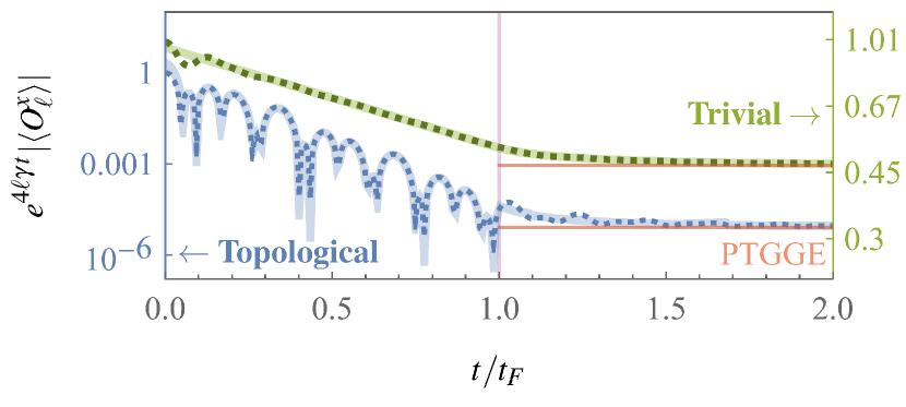
Figure 8: Dual string order parameter after quenches to the trivial (green, $\Delta J=0.5J$) and topological (blue, $\Delta J=-0.5J$) PT-symmetric phases for $\gamma=\Delta\gamma=0.3J$, $\delta=\Delta=0$, and $\ell=20$. Dashed lines correspond to numerical data, and the solid lines show the analytical conjectures in Eqs. (161) and (162) with $\alpha_{+}=\alpha_{-}=0.15$. We indicate the asymptotic PTGEE prediction by straight horizontal red lines and the the change of dynamics at the characteristic time scale $t=t_{F}$ by the purple vertical line. The system size $L$ is chosen sufficiently large to avoid finite-size effects.

To illustrate relaxation to the PTGGE, we consider the time evolution of the dual string order parameter after quenches to the trivial and topological PT-symmetric phases. As discussed in Sec. IV.1.1, the expectation value of a product of $\ell$ fermionic operators becomes stationary after rescaling with a factor of $e^{2\ell\gamma t}$. Accordingly, in Fig. 8, we show the evolution of the rescaled dual string order parameter $e^{4\ell\gamma t}\left\lvert\langle O_{\ell}^{x}\rangle\right\rvert$. For quenches to both the topological (blue) and the trivial (green) phase, we observe fast decay up to the Fermi time $t_{F}$ Eq. (152), followed by much slower relaxation to the value predicted by the PTGGE. As an aside, it is interesting to note that, since $G_{2,\ell}$ does not contribute to $\Gamma_{\ell}$ in Eq. (159), relaxation of the dual string order parameter is described by the PTGGE even if $\delta,\Delta\neq 0$. The numerical data for the quench to the trivial phase is in excellent agreement with the following analytical form:

$$\langle O^{x}_{\ell}(t)\rangle\sim O_{0}e^{-4\ell\gamma t+\int_{0}^{\pi}\frac{dk}{2\pi}\min(2\left\lvert v_{k}\right\rvert t,\ell)\mathop{\mathrm{tr}}\left(\ln\left(\left\lvert\zeta_{k}^{\prime}f_{k}^{-1}\right\rvert\right)\right)},$$ (161)

where $\zeta_{k}^{\prime}$ and $f_{k}$ are defined in Eqs. (133) and (120), respectively, and the prefactor $O_{0}$ is determined by fitting the late-time asymptotic behavior to the PTGGE prediction. Equation (161) is an analytical conjectures we have proposed originally for the dynamics of the subsystem parity in the driven-dissipative Kitaev chain [37], and which is based on analytical results obtained by Calabrese et al. [13, 14, 15] for the relaxation of order parameter correlations in the transverse field Ising model and in the space-time scaling limit $\ell,t\to\infty$ with $\ell/t$ fixed. As mentioned above, the SSH model can be mapped to two coupled Ising models by a nonlocal unitary transformation [101], which leads us to expect that our conjecture also applies to the dual string order parameter. Numerically, this expectation is confirmed in Fig. 8, where the solid lines indicate the analytical predictions.

The analytical conjecture Eq. (161) shows that as compared to the isolated SSH model, there are two important modifications: (i) The dynamics are determined the Liouvillian dispersion relation $\omega_{k}$ rather than the Hamiltonian dispersion relation $\varepsilon_{k}$, leading here to a shorter Fermi time $t_{F}$; (ii) noncanonical anticommuation relations of Liouvillian quasiparticles encoded in $f_{k}\neq\mathbbm{1}$ affect the result quantitatively.

For quenches to the topologically nontrivial phase with $\Delta J<0$, the dual string order parameter exhibits additional oscillatory dynamics for $t<t_{F}$, well described in the space-time scaling limit by

$$\langle O^{x}_{\ell}(t)\rangle\sim 2\cos(\omega_{k_{s,+}}t+\alpha_{+})\cos(\omega_{k_{s,-}}t+\alpha_{-})\langle O^{x}_{\ell}(t)\rangle_{\mathrm{nonosc}},$$ (162)

where $\langle O^{x}_{\ell}(t)\rangle_{\mathrm{nonosc}}$ is the nonoscillatory evolution described by Eq. (161), $\alpha_{\pm}$ are numerically determined phase shifts, and $k_{s,\pm}$ are the soft modes of the PTGGE. These modes are determined by the condition that the matrix in the exponent in Eq. (77) has an eigenvalue that is equal to zero. According to Eq. (132), this condition can be stated as

$$\det\!\left(g_{\mathrm{PTGGE},k}(t)\right)=e^{-8\gamma t}\det\!\left(V_{k}^{-\dagger}V_{k}^{-1}\right)\det\!\left(\zeta_{k}^{\prime}\right)\\ =-\frac{\varepsilon_{k}^{2}}{\omega_{k}^{2}}e^{-8\gamma t}\cos(\Delta\phi_{k}-\psi_{k})\cos(\Delta\phi_{k}+\psi_{k})=0,$$ (163)

or, equivalently, $\cos(\Delta\phi_{k}\pm\psi_{k})=0$. As we show below, $\cos(\Delta\phi_{k}-\psi_{k})=0$ has two solutions $k=k_{s,\pm}$. The solutions to $\cos(\Delta\psi_{k}+\psi_{k})=0$ are then given by $-k_{s,\pm}$: Indeed, IS of the Bloch Hamiltonian $h_{k}$ and IS^† of the non-Hermitian Bloch Hamiltonian $z_{k}$ imply that $\Delta\phi_{k}=-\Delta\phi_{k}$ and $\psi_{k}=\psi_{-k}$, respectively [37], and, therefore, $\cos\!\left(\Delta\phi_{-k_{s,\pm}}+\psi_{-k_{s,\pm}}\right)=\cos\!\left(\Delta\phi_{k_{s,\pm}}-\psi_{k_{s,\pm}}\right)=0$. It is thus sufficient to consider the condition $\cos(\Delta\phi_{k}-\psi_{k})=0$. For our choice of initial state with vanishing intercell hopping, $J_{2,0}=0$, this condition leads to

$$J_{1}+J_{2}\cos(k)=-\mathop{\mathrm{sgn}}(\sin(k))2\Delta\gamma,\quad\omega_{k}=J_{2}\left\lvert\sin(k)\right\rvert.$$ (164)

The two solutions are given by

$$k_{s,\pm}=\mp\mathop{\mathrm{sgn}}(J_{1})\arccos\!\left(-\left(J_{1}\mp\mathop{\mathrm{sgn}}(J_{1})2\Delta\gamma\right)\middle/J_{2}\right).$$ (165)

We have chosen the designation of each of the solutions of Eq. (164) as either $k_{s,+}$ or $k_{s,-}$ such that $k_{s,-}$ and $k_{s,+}$ are associated with the pumping of string order through the right and left boundary of a subsystem, respectively, as detailed below. Note that the designation is reversed when $J_{1}=J+\Delta J$ changes sign. Crucially, for this choice, the frequencies $\omega_{k_{s,\pm}}$ are continuous functions of $\Delta J$ and $\Delta\gamma$. For $\Delta\gamma\neq 0$, the PTGGE has two distinct soft modes $k_{s,+}\neq-k_{s,-}$. In contrast, for the GGE, which is obtained for $\Delta\gamma\to 0$, the soft modes are locked onto each other by inversion symmetry, $k_{s,+}=-k_{s,-}$. Associated with the soft modes are two time scales ,

$$t_{s,\pm}=\pi/\omega_{k_{s,\pm}}=\left.\pi\middle/\left(J_{2}\left\lvert\sin(k_{s,\pm})\right\rvert\right),\right.$$ (166)

which determine the oscillation periods of the dual string order parameter, and, in particular, the periodicity of the recurring zero crossings of the dual string order parameter. Note that since $\omega_{k}=\omega_{-k}$, there is only a single time scale $t_{s}=t_{s,+}=t_{s,-}$ for isolated systems. As shown in Fig. 8, the periodicity of zero crossings persists up to $t_{F}$, and the subsequent relaxation of the dual string order parameter for $t>t_{F}$ approximately follows the prediction given in Eq. (161).

The oscillatory dynamics of the dual string order parameter for quenches to the topological phase are connected to the topological zero crossings in the entanglement spectrum. We explore this connection in more detail in the following section.

VII.1.2 Topological zero crossings

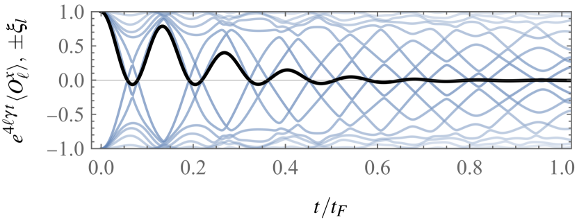
Figure 9: Simultaneous zero crossings of the dual string order parameter (black line) and in the single-particle entanglement spectrum (blue lines) for a quench to the topological phase, $\Delta J=-1.5J$ and $\gamma=\Delta\gamma=0.3J$, with balanced loss and gain $\delta=\Delta=0$, and for a subsystem of size $\ell=10$.

For quantum quenches in the isolated SSH model, zero crossings of the dual string order parameter are a robust signature of the topology of the postquench Hamiltonian. To explain why that is the case, we observe first that according to Eq. (157) zero crossings of the dual string order parameter occur whenever an eigenvalue of $\Gamma_{\ell}$, or, equivalently as per Eq. (159), of the reduced covariance matrix $G_{\ell}$, crosses zero. The coincidence of zero crossings of the dual string order parameter and in the single-particle entanglement spectrum applies to all Gaussian states, and is illustrated for a quench to the topological PT-symmetric phase in Fig. 9. Furthermore, the dynamical entanglement spectrum bulk-boundary correspondence for one-dimensional lattice models [4] that belong to the class BDI [108] states that for quenches originating from the trivial phase, zero crossings in the entanglement spectrum occur if and only if the postquench Hamiltonian is topologically nontrivial. Consequently, also zero crossings of the dual string order parameter occur if and only if the postquench Hamiltonian of the isolated SSH model is topologically nontrivial. As we discuss in more detail below, for the Kitaev chain, the role of the dual string order parameter is played by the subsystem fermion parity [37].

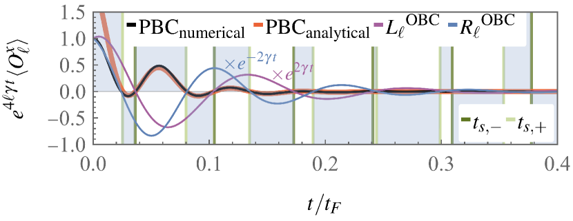
Figure 10: Directional string order pumping for a quench to the topological PT-symmetric phase with $\Delta J=-0.5J$, $\gamma=\Delta\gamma=0.2J$, $\delta=\Delta=0$, and $\ell=40$. For PBC, the numerical data (black line) crosses zero at multiples of both $t_{s,+}$ (light green) and $t_{s,-}$ (dark green), with blue shading indicating the sign of the dual string order parameter. The analytical conjecture Eq. (162) agrees well with the numerics (red line). For OBC, zero crossings occur at multiples of $t_{s,-}$ or $t_{s,+}$ depending on whether the subsystem is at the left ($L_{\ell}$, violet line) or the right end of the chain ($R_{\ell}$, blue line). Additional rescaling with $e^{\pm 2\gamma t}$ of the data for $L_{\ell}$ and $R_{\ell}$ compensates for exponential decay and growth, respectively, due to edge modes.

Turning now to the driven-dissipative SSH model, the continuity of non-Hermitian real-line-gap topology suggests that the relation between zero crossings of the dual string order parameter and nontrivial topology of the generator of the postquench dynamics remains valid through the entire PT-symmetric phase. An important qualitative modification due to drive and dissipation has already been mentioned above: There are now two distinct time scales for zero crossings of the dual string order parameter, which are determined by soft modes of the PTGGE. In Ref. [37], for the driven-dissipative Kitaev chain, we have provided a physical interpretation of these two time scales in terms of directional parity pumping: The two time scales correspond to different rates of the exchange of parity between a subsystem and its complement through the left and right ends of the subsystem. This effect requires the breaking of inversion symmetry and mixedness of the time-evolved state, and is thus unique to driven-dissipative systems. As we illustrate in Fig. 10, the driven-dissipative SSH model exhibits an analogous effect of directional string order pumping. The figure shows the dynamics of the rescaled dual string order parameter for a quench to the PT-symmetric topological phase. After a short initial period, the numerical data for PBC (black line) are well described by the analytical prediction Eq. (162) (red line), and exhibit zero crossings at multiples of both $t_{s,-}$ and $t_{s,+}$. In contrast, the dual string order parameter for subsystems $L_{\ell}=\{1,\dots,\ell\}$ at the left end and $R_{\ell}=\{L-\ell+1,\dots,L\}$ at the right end of a chain with OBC, crosses zero at multiples of only $t_{s,-}$ and $t_{s,+}$, respectively. These observations confirm that string order pumping does indeed occur at different rates through the left and right ends of a subsystem. We note that a previous study of topological entanglement spectrum crossings in the driven-dissipative Kitaev chain has focused on subsystems of type $L_{\ell}$ and has, therefore, not observed directional pumping [86].

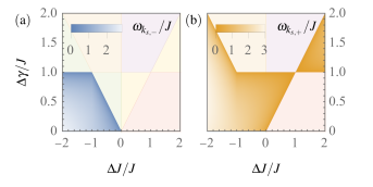
Figure 11: Directional string order pumping phase diagram of the driven-dissipative SSH model determined by the soft-mode frequencies (a) $\omega_{k_{s,-}}$ and (b) $\omega_{k_{{s,+}}}$. The phases determined by PT symmetry, introduced in Fig. 2, are shown in the background.

As explained above, our expectation for the occurrence of zero crossings of the dual string order parameter in the topological PT-symmetric phase is based on the continuity of topological properties throughout this phase. Indeed, for the driven-dissipative SSH model, two soft modes $k_{s,\pm}$ of the PTGGE given by Eq. (165) exist within the entire topological PT-symmetric phase. The corresponding frequencies $\omega_{k_{s,\pm}}$ are shown in Fig. 11. Upon increasing $\Delta\gamma$, one of the soft mode frequencies, $\omega_{s,-}$, vanishes at the transition from the PT-symmetric to the PT-mixed phase. In contrast, $\omega_{k_{s,+}}$ remains finite within the entire PT-mixed phase, and vanishes at the boundaries separating the PT-mixed from the trivial PT-symmetric and the PT-broken phases. This observation suggests that zero crossings of the dual string order parameter can also occur in the PT-mixed phase—an expectation that is confirmed in Fig. 12. The numerical analysis of zero crossings of the dual string order parameter for quenches to the PT-mixed phase is more challenging than for the PT-symmetric phase: In the PT-symmetric phase, through a simple rescaling, the overall exponential decay of the covariance matrix can be removed analytically before evaluating the covariance matrix numerically [37]. In contrast, due to the finite bandwidth of decay rates in the PT-mixed phase, exponential decay cannot be fully accounted for beforehand, leading at late times to extremely small numbers below the numerical precision. The data shown in Fig. 12 is rescaled by $e^{\left(4\ell\gamma_{s}+c\right)t}$, where $2\gamma_{s}$ is the decay rate of the slowest-decaying PT-breaking mode given in Eq. (145), and we have chosen $c=51$ to best present the numerical results. In agreement with our expectations based on the values of $\omega_{k_{s,\pm}}$ shown in Fig. 11, the dual string order parameter for the subsystem $L_{\ell}$ does not exhibit zero crossings, while for $R_{\ell}$ there are zero crossings at multiples of $t_{s,+}$. Note that the numerical data for $R_{\ell}$ stops abruptly due to the occurrence of exponentially small numbers in the calculation of the Pfaffian. For PBC we, further observe a transition from a fast initial decay to a much slower relaxation behavior, in analogy to but much smoother than the transition at $t_{F}$ for the quenches to the PT-symmetric phase shown in Fig. 8.

Our findings lead us to speculate that the non-Hermitian topology of a suitably defined restriction of the matrix $z_{k}$ to its PT-symmetric eigenmodes remains intact even upon crossing the transition to the PT-mixed phase, and that a finite gap is not essential for such a construction. In physical terms, our results suggest to define directional pumping phases based on the existence of soft modes. For the driven-dissipative SSH model, as can be seen in Fig. 11, the phase boundaries of directional pumping phases are also phase boundaries in terms of the gap structure and PT symmetry. However, as we discuss for the example of a driven-dissipative Kitaev chain with long-range hopping and pairing in Sec. VIII below, this does not have to be the case.

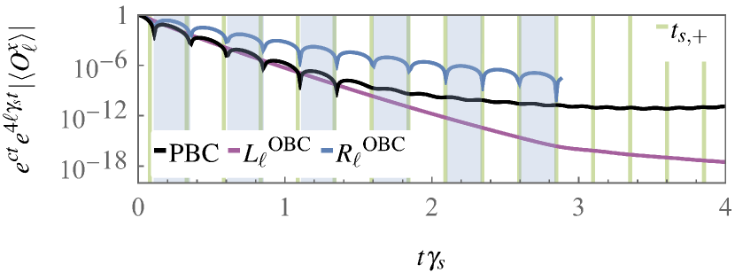
Figure 12: Directional string order pumping for quenches to the PT-mixed phase with $\Delta J=-5J$, $\Delta\gamma=\gamma=1.1J$, and $\ell=30$, for PBC (black line) and for OBC with subsystems located at the left ($L_{\ell}$, purple line) and the right edge of the chain ($R_{\ell}$, blue line). The blue shading indicates the sign of the dual string order parameter for the subsystem $R_{\ell}$. Zero crossings of the dual string order parameter for PBC and the subsystem $R_{\ell}$ for OBC fit well to the soft mode time scale $t_{s,+}$. We include an additional exponential rescaling $e^{ct}$ with $c=51$ to improve the presentation of the data.

VII.1.3 Dynamical criticality

Having introduced the concept of directional pumping phases, we may ask what kind of critical behavior occurs at the transitions between these phases, and whether this behavior is universal. Usually, dynamical critical phenomena in driven-dissipative systems are associated with symmetry-breaking second order phase transitions in the steady state [24, 25, 26, 27, 28, 29, 30, 31, 32]. Then, critical behavior is induced by the closing of the dissipative gap, given by the decay rate of the slowest-decaying eigenmode of the Liouvillian, at the critical point. In particular, the correlation length diverges as $\xi\sim\left\lvert\delta_{g}\right\rvert^{-\nu}$, where $\delta_{g}=g-g_{c}$ is the deviation of the parameter $g$ from its critical value $g_{c}$, and the divergence of the relaxation time scale $\tau\sim\left\lvert\delta_{g}\right\rvert^{-\nu z}$, where $z$ is the dynamical critical exponent, leads to the phenomenon of critical slowing down. Contrary to that, directional pumping phase transitions mark a qualitative change in the oscillatory dynamics of the dual string order parameter and are not associated with any changes in the steady state. Indeed, we consider here dynamics which, for $\delta=\Delta=0$, always lead to a steady state at infinite temperature with a vanishing correlation length. Further, the rate of relaxation to the steady state is finite for any value of $\gamma>0$. Instead, directional pumping phase transitions are characterized by divergences of the soft-mode time scales $t_{s,\pm}$, which determine the periodicity of zero crossings of the dual string order parameter. The soft modes $k_{s,\pm}$ and the associated time scales $t_{s,\pm}$ are genuinely dynamical quantities and depend on both pre- and postquench parameters. However, as we discuss in the following, the critical exponents that govern the power-law behavior of $k_{s,\pm}$ and $t_{s,\pm}$ at the phase boundaries do not depend on the specific choice of parameters. These exponents are determined by an effective long-wavelength description, which indicates that their values are indeed universal.

At the boundaries of the directional pumping phases, the soft modes $k_{s,\pm}$ approach values $k_{s,\pm,c}$. The frequencies $\omega_{k_{s,\pm}}=J_{2}\,\lvert\sin(k_{s,\pm})\rvert$ vanish at the phase boundaries, implying that $k_{s,\pm,c}=0,\pm\pi$. In analogy to the correlation length exponent $\nu$ and the dynamical exponent $z$, we define critical exponents $\nu^{\prime}$ and $z^{\prime}$ through the scaling behavior

$$\left\lvert k_{s,\pm}-k_{s,\pm,c}\right\rvert\sim\left\lvert\delta_{g}\right\rvert^{\nu^{\prime}},\qquad\omega_{k_{s,\pm}}\sim\left\lvert\delta_{g}\right\rvert^{\nu^{\prime}z^{\prime}},$$ (167)

for $\delta_{g}=g-g_{c,\pm}\to 0$, leading to a divergence of the soft-mode time scales $t_{s,\pm}\sim\left\lvert\delta_{g}\right\rvert^{-\nu^{\prime}z^{\prime}}$. For the SSH model, we consider the parameters $g=\Delta J$ and $g=\Delta\gamma$. Let us assume that the values $\Delta J_{c,\pm}$ and $\Delta\gamma_{c,\pm}$ correspond to a particular point on the phase boundary of $\omega_{k_{s,\pm}}$, where $k_{s,\pm}$ takes the value $k_{s,\pm,c}$. To obtain the behavior of $k_{s,\pm}$ and $\omega_{k_{s,\pm}}$ in the vicinity of this critical point, we set $\Delta J=\Delta J_{c,\pm}+\delta_{\Delta J}$ and $\Delta\gamma=\Delta\gamma_{c,\pm}+\delta_{\Delta\gamma}$ in Eq. (164), and expand in $k$ around $k_{s,\pm,c}$. We thus find

$$\left\lvert k_{s,\pm}-k_{s,\pm,c}\right\rvert\sim\omega_{k_{s,\pm}}\sim\left\lvert\delta_{g}\right\rvert^{1/2}\quad\text{for }\delta_{g}\to 0,$$ (168)

for both $g=\Delta J$ and $g=\Delta\gamma$. Therefore, the time scales $t_{s,\pm}$ exhibit a square-root divergence with critical exponents

$$\nu^{\prime}=1/2,\qquad z^{\prime}=1,$$ (169)

irrespective of the direction from which the phase boundary is approached in the $\Delta J$-$\Delta\gamma$ plane.

VII.2 Subsystem fermion parity

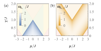
Figure 13: Directional parity pumping phases determined by the soft-mode frequencies (a) $\omega_{k_{s,-}}$ and (b) $\omega_{k_{s,+}}$ for the driven-dissipative Kitaev chain. The background colors indicate the phases defined by PT symmetry, with PT-symmetric phases (blue, red), PT-mixed phases (green, yellow) and a PT-broken phase (orange) [86, 37].

As mentioned above, the subsystem fermion parity serves as a topological disorder parameter for the Kitaev chain. This can be seen by noting that a combination of the Jordan-Wigner [98] and Kramers-Wannier [109, 110] transformations maps the Kitaev chain to the transverse field Ising model such that the trivial phase of the Kitaev chain corresponds to the ferromagnetically ordered phase of the Ising model. Then, order-parameter correlations of the Ising model over a distance $\ell$ are equivalent to the fermion parity $P_{\ell}$ of a subsystem of size $\ell$ of the Kitaev chain [37], which is defined by

$$P_{\ell}=e^{i\pi\sum_{l=1}^{\ell}c_{l}^{\dagger}c_{l}}.$$ (170)

For a Gaussian state, the expectation value $\langle P_{\ell}\rangle=\mathop{\mathrm{pf}}(\Gamma_{\ell})$ is given by the Pfaffian of the reduced covariance matrix $\Gamma_{\ell}$ defined in Eq. (64) [102, 103, *Barouch1971II, *Barouch1971III].

VII.2.1 Topological zero crossings

In complete analogy to our the discussion for the SSH model in Sec. VII.1.2, the subsystem parity can be seen to exhibit zero crossings for quenches of the isolated Kitaev chain from the trivial to the topological phase. As shown in Refs. [37], the connection between zero crossings and topology remains valid throughout the entire PT-symmetric phase of the driven-dissipative Kitaev chain. The periodicities $t_{s,\pm}$ of these zero crossings are determined by the soft modes $k_{s,\pm}$, which, for $\mu_{0}\to-\infty$, are given by the solutions to [37]

$$2J\cos(k)+\mu=\mathop{\mathrm{sgn}}(\sin(k))2\gamma,\quad\omega_{k}=2\Delta\left\lvert\sin(k)\right\rvert.$$ (171)

We find

$$k_{s,\pm}=\pm\mathop{\mathrm{sgn}}(\mu)\arccos\!\left(-\left(\mu\mp\mathop{\mathrm{sgn}}(\mu)2\gamma\right)\middle/\left(2J\right)\right),$$ (172)

and the corresponding frequencies $\omega_{k_{s,\pm}}$ determine the directional pumping phases shown in Fig. 13. As in the case of the SSH model, the frequency $\omega_{k_{s,-}}$, which describes parity pumping through the right end of a subsystem, is nonzero only within the topological PT-symmetric phase; in contrast, the frequency $\omega_{k_{s,+}}$, corresponding to parity pumping through the left end of a subsystem, remains finite within the entire PT-mixed phase. The phase boundaries defined by directional parity pumping coincide with those that are related to PT symmetry. However, as we show in Sec. VIII.1 where we consider a Kitaev chain with long-range hopping and pairing, this does not have to be the case.

VII.2.2 Dynamical criticality

The critical exponents $\nu^{\prime}$ and $z^{\prime}$, which describe the behavior of the soft modes $k_{s,\pm}$ and the frequencies $\omega_{k_{s,\pm}}$ in the vicinity of transitions between directional pumping phases according to Eq. (167), take on the same values for the Kitaev chain as for the SSH model. To obtain this result, we insert $\mu=\mu_{c}+\delta_{\mu}$ and $\gamma=\gamma_{c}+\delta_{\gamma}$ in Eq. (171) and expand in $k$ around $k_{s,\pm,c}=0,\pm\pi$. We obtain

$$\omega_{k_{s,\pm}}\sim\left\lvert k_{s,\pm}-k_{s,\pm,c}\right\rvert\sim\left\lvert\delta_{g}\right\rvert^{1/2}\quad\text{for }\delta_{g}\to 0,$$ (173)

for both $g=\mu$ and $g=\gamma$, which leads to the values of $\nu^{\prime}$ and $z^{\prime}$ given in Eq. (169). As we show in the next section, the values of these exponents can be modified in the presence of long-range hopping and pairing.

VIII Driven-dissipative Kitaev chain with long-range hopping and pairing

We have introduced the concept of directional pumping phases to distinguish parameter regions with qualitatively different dynamics of string order and fermion parity. Transitions between directional pumping phases are characterized by divergent time scales $t_{s,\pm}$ for string order and parity pumping, and there is evidence for universality of the exponents that govern the critical behavior of $t_{s,\pm}$: We have found the same exponents given in Eq. (169) for two models that differ by the presence of a weak $\mathrm{U}(1)$ symmetry but belong to the same Altland-Zirnbauer class; and these exponents can be obtained from an expansion in momenta around critical values $k_{s,\pm,c}$, which indicates that models with the same low-momentum or, equivalently, long-wavelength description will have the same exponents, while microscopic details that require the entire Brillouin zone for their description are irrelevant. However, in the examples we have considered so far, the boundaries of directional pumping phases coincide with gap closings of the Liouvillian single-particle spectrum in the complex plane, suggesting that also directional pumping phase transitions are a mere manifestation of gap closings, and that the exponents that describe the critical behavior of $t_{s,\pm}$ are determined by those that govern the divergences of oscillation periods of low-order correlation functions [86]. To better understand the relation between directional pumping phases and the more elementary notion of dynamical phases defined in terms of gap closings or PT symmetry, we now consider quench dynamics in a Kitaev chain with long-range hopping and pairing [111, 112, 113, 114, 115, 116, 117, 118, 119, 120, 121, 122, 123, 124, 125, 126, 127]. Long-range couplings are known to modify critical properties at gap closings in isolated systems. As we discuss in the following, for a Kitaev chain with Markovian drive and dissipation, the presence of long-range couplings can likewise lead to modifications of the critical exponents that are associated with the pumping time scales $t_{s,\pm}$, but does not affect the exponents that govern the divergence of the oscillation period of the density autocorrelation function. Furthermore, even the boundaries of the directional pumping phases of the driven-dissipative long-range Kitaev chain do not always coincide with gap closings. These results indicate that directional pumping phases and the associated critical behavior are indeed new and independent concepts.

VIII.1 Long-range Kitaev chain

We consider a Kitaev chain with long-range hopping and pairing as described by the Hamiltonian [125]

$$H=\sum_{l=1}^{L}\sum_{r=1}^{\lfloor L/2\rfloor}\left(-J_{r}c^{\dagger}_{l}c_{l+r}+\Delta_{r}c_{l}c_{l+r}+\mathrm{H.c.}\right)\\ -\mu\sum_{l=1}^{L}\left(c^{\dagger}_{l}c_{l}-\frac{1}{2}\right),$$ (174)

where both the hopping matrix element $J_{r}=\left.J\middle/\left(\mathcal{N}_{\alpha}r^{\alpha}\right)\right.$ and the pairing amplitude $\Delta_{r}=\left.\Delta\middle/\left(\mathcal{N}_{\alpha}r^{\alpha}\right)\right.$ decay with distance as a power law with exponent $\alpha>1$, and the Kac normalization factors are defined as $\mathcal{N}_{\alpha}=\sum_{r=1}^{\lfloor L/2\rfloor}r^{-\alpha}$ [128]. As with the short-range Kitaev chain, we assume that the coupling to Markovian reservoirs is described by the jump operators given in Eq. (61), where we focus on $\gamma_{l}=\gamma_{g}$ in this section. Consequently, the single-particle dispersion relation of the Liouvillian takes the form given in Eq. (65), but with the Hamiltonian dispersion relation $\varepsilon_{k}$ given by

$$\varepsilon_{k}=\sqrt{\left(2J_{k}+\mu\right)^{2}+4\Delta_{k}^{2}},$$ (175)

where, in the thermodynamic limit $L\to\infty$,

$$J_{k}=\frac{J}{\zeta\!\left(\alpha\right)}\mathop{\mathrm{Re}}\!\left(\mathrm{Li}_{\alpha}\!\left(e^{ik}\right)\right),\quad\Delta_{k}=\frac{\Delta}{\zeta\!\left(\alpha\right)}\mathop{\mathrm{Im}}\!\left(\mathrm{Li}_{\alpha}\!\left(e^{ik}\right)\right).$$ (176)

Explicit expressions for the polylogarithm $\mathrm{Li}_{\alpha}(z)$ and the Riemann zeta function $\zeta(\alpha)$ are provided in Appendix D.

VIII.2 Phase diagram of the long-range Kitaev chain

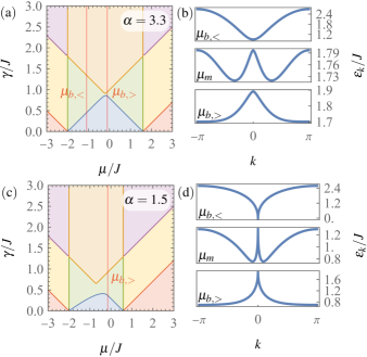
Figure 14: Phase diagrams and dispersion relations of the long-range Kitaev chain for (a), (b) $\alpha=3.3$ and (c), (d) $\alpha=1.5$. (a), (c) Colors indicate PT-symmetric (blue, red), PT-mixed (green, yellow) and PT-broken phases (orange, purple). (b), (d) Dispersion relations $\varepsilon_{k}$ with a single minimum at $k=0$ for $\mu=\mu_{b,<}$, two degenerate minima at $k=\pm k_{b}$ for $\mu=\mu_{m}$, and a single minimum at $k=\pi$ for $\mu=\mu_{b,>}$. The bifurcation points $\mu_{b,\lessgtr}$ are shown in (a), (c) as red lines. For $\alpha=1.5$, the first bifurcation occurs at $\mu_{b,<}=\mu_{c,<}=-2J$.

Long-range couplings do not affect the symmetry properties of the Kitaev chain; in particular, the driven-dissipative long-range Kitaev chain is PT-symmetric. The phase diagram of the long-range Kitaev chain, determined by the spontaneous breaking of PT symmetry, is shown in Figs. 14(a) and (c) for $\alpha=3.3$ and $\alpha=1.5$, respectively. In comparison to the phase diagram of the short-range Kitaev chain [37, 86], the key qualitative differences are the absence (i) of mirror symmetry with respect to axis $\mu=0$ and (ii) of a direct transition between the PT-symmetric and the PT-broken phase, and (iii) a segment of the boundary of the topological PT-symmetric phase being curved instead of described by straight lines.

To understand these modifications, let us first discuss how the corresponding properties come about in the short-range Kitaev chain: (i) The unitary transformation $c_{l}\mapsto\left(-1\right)^{l}c_{l}$ maps the Hamiltonian $H$ Eq. (60) and the chemical potential $\mu$ to $-H$ and $-\mu$, respectively. Therefore, gap closings that determine phase boundaries occur symmetrically with respect to $\mu=0$. This symmetry of the isolated Kitaev chain extends to the driven-dissipative model. However, in the isolated long-range Kitaev chain, the mapping $c_{l}\mapsto\left(-1\right)^{l}c_{l}$ does not result in a simple sign change and, therefore, the phase diagram does not have reflection symmetry with respect to $\mu=0$. The critical values $\mu_{c,\lessgtr}$ of the chemical potential that separate the topological phase from the trivial phase are given by

$$\mu_{c,<}=-2J_{0}=-2J,\quad\mu_{c,>}=-2J_{\pi}=2J\eta(\alpha)/\zeta(\alpha).$$ (177)

We note that also the midpoint between $\mu_{c,<}$ and $\mu_{c,>}$, given by $\mu_{m}=-\left(J_{\pi}+J_{0}\right)$, does not describe a mirror symmetry of the phasediagram, but will prove to be convenient in the characterization of the long-range Kitaev chain.

(ii) At $\mu=0$, the dispersion relation of the short-range Kitaev chain is flat, $\varepsilon_{k}=2\sqrt{J^{2}+\Delta^{2}}$. Therefore, upon increasing $\gamma$, the Liouvillian dispersion relation Eq. (65) becomes imaginary simultaneously for all $k\in\mathrm{BZ}$, leading to a direct transition from the PT-symmetric to the PT-broken phase. In contrast, for $1<\alpha<\infty$, the dispersion relation Eq. (175) of the long-range Kitaev chain is never flat. The resulting absence of a direct transition between the PT-symmetric and PT-broken phase is clearly visible in Fig. 14.

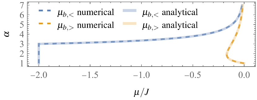
Figure 15: Numerical evaluation of the left and right bifurcation points $\mu_{b,<}$ (blue, dashed) and $\mu_{b,>}$ (orange, dashed), respectively, together with the analytical predictions in Eqs. (179) and (181) (blue, solid) and (178) (orange, solid).

(iii) Spontaneous breaking of PT symmetry, which determines the boundary of the PT-symmetric phase, occurs when $\omega_{k}$ Eq. (65) where $\gamma=\gamma_{l}=\gamma_{g}$ with $\varepsilon_{k}$ given in Eq. (175) becomes imaginary for some $k$. This happens when $\min_{k\in\mathrm{BZ}}(\varepsilon_{k})=2\gamma$. For the short-range Kitaev chain, the dispersion relation $\varepsilon_{k}$ takes its minimum value at $k_{\mathrm{min}}=0$ when $\mu<0$, and at $k_{\mathrm{min}}=\pi$ when $\mu>0$; the jump of $k_{\mathrm{min}}$ from $0$ to $\pi$ occurs at $\mu=0$ where the dispersion is flat. In contrast, in the long-range Kitaev chain with $1<\alpha<\infty$, there are two bifurcation points of the minimum of $\varepsilon_{k}$ at $\mu_{b,\lessgtr}$: There is a single minimum at $k=0$ for $\mu<\mu_{b,<}$; then, in the range $\mu_{b,<}<\mu<\mu_{b,>}$, there are two degenerate minima at momenta $\pm k_{b}$ with $k_{b}$ increasing monotonically from 0 to $\pi$ for $\mu$ increasing from $\mu_{b,<}$ to $\mu_{b,>}$; finally, for $\mu_{b,>}<\mu$, there is again a single minimum at $k=\pi$. This is illustrated for $\alpha=3.3$ and $\alpha=1.5$ in Figs. 14(b) and (d), respectively. To determine the precise shape of the phase boundary, we note that $\Delta_{k}$ defined in Eq. (176) vanishes at $k=0,\pi$. Therefore, for $\mu<\mu_{b,<}$ and $\mu_{b,>}<\mu$, the boundary of the PT-symmetric phase is determined by $\varepsilon_{0}=\left\lvert 2J_{0}+\mu\right\rvert=2\gamma$ and $\varepsilon_{\pi}=\left\lvert 2J_{\pi}+\mu\right\rvert=2\gamma$, respectively. These conditions describe straight lines and are symmetric with respect to $\mu_{m}$ defined above. But for $\mu_{b,<}<\mu<\mu_{b,>}$, PT symmetry breaking occurs for $\varepsilon_{k_{b}}=2\gamma$, yielding a smaller critical value of $\gamma$ as compared to an extension of the straight boundaries over the entire range of values of $\mu$.

The momenta $\pm k_{b}$ at which the dispersion relation takes on its minimum value for $\mu_{b,<}<\mu<\mu_{b,<}$ can only be found numerically. However, the bifurcation points $\mu_{b,\lessgtr}$ can be found analytically by using the series expansions of the polylogarithm given in Appendix D: To determine the right bifurcation point $\mu_{b,>}$, we employ the expansion of $\varepsilon_{k}$ around $k=\pi$ given by $\varepsilon_{k}\sim\varepsilon_{\pi}+(k-\pi)^{2}/(2m_{\pi})$, and solve the equation $1/m_{\pi}=0$ for $\mu$. Using Eq. (233), for $1<\alpha<\infty$, we find

$$\mu_{b,>}=-2\left[J_{\pi}+\left.\left(\Delta_{\pi}^{\prime}\right)^{2}\middle/J_{\pi}^{\prime\prime}\right.\right],$$ (178)

where primes denote derivatives with respect to $k$. The left bifurcation point $\mu_{b,<}$ is determined by $\varepsilon_{k}\sim\varepsilon_{0}+k^{2}/(2m_{0})$ and $1/m_{0}=0$, which holds for $3<\alpha<\infty$, where the term $\sim k^{\alpha-1}$ in Eq. (231) can be neglected. We obtain

$$\mu_{b,<}=-2\left[J_{0}+\left.\left(\Delta_{0}^{\prime}\right)^{2}\middle/J_{0}^{\prime\prime}\right.\right]\quad\text{for }3<\alpha<\infty.$$ (179)

For $1<\alpha<3$, using the same idea as above but keeping only the relevant terms in the expansion in Eq. (231), we are led to

$$\frac{\left(\Delta^{\prime}_{k}\right)^{2}}{J^{\prime\prime}_{k}}\propto\frac{\left(k^{\alpha-2}+c_{1}\right)^{2}}{k^{\alpha-3}+c_{2}}\xrightarrow{k\to 0}0,$$ (180)

where $c_{1},c_{2}\in\mathbb{R}$ are constants. Therefore,

$$\mu_{b,<}=-2J_{0}\qquad\text{for }1<\alpha<3.$$ (181)

In Fig. 15, our analytical expressions for the bifurcation points are shown to agree with numerical solutions.

VIII.3 Subsystem fermion parity

The time evolution of the subsystem parity after quenches to the topological PT-symmetric phase for $\alpha=2.5$ and $\alpha=1.5$ is shown in Fig. 16. In comparison to the short-range Kitaev chain with Markovian drive and dissipation, there are more pronounced oscillations after $t=t_{F}$. However, the stationary values of the rescaled subsystem parity are still well described by the PTGGE.

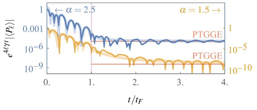
Figure 16: Relaxation of the subsystem parity after quenches in the driven-dissipative Kitaev chain with long-range couplings. Both quenches are to the topological phase, where the blue line corresponds to $\alpha=2.5$, $\mu=-J$, $\gamma=0.3J$, and $\ell=20$, and the orange line to $\alpha=1.5$, $\mu=-0.5J$, $\gamma=0.15J$, and $\ell=80$. Thin and thick lines show numerical data and the analytical conjecture in Eq. (162), respectively. For smaller values of $\alpha$ corresponding to longer-range couplings, finite-size effects are more strongly pronounced and larger system sizes are required. The purple vertical line indicates the characteristic relaxation time scale $t_{F}$ and the red horizontal lines show the PTGGE predictions.

VIII.3.1 Topological zero crossings

The time scale of topological zero crossings of the subsystem parity is determined by soft modes of the PTGGE. In the presence of long-range couplings, the conditions Eq. (171), which determine the soft modes and associated frequency scales for the short-range Kitaev chain, are generalized to

$$2J_{k}+\mu=\mathop{\mathrm{sgn}}(\Delta_{k})2\gamma,\quad\omega_{k}=2\left\lvert\Delta_{k}\right\rvert.$$ (182)

To solve these equations, we use the following properties of the function $J_{k}$ and $\Delta_{k}$ defined in Eq. (176), which hold for $1<\alpha<\infty$: (i) $J_{k}=J_{-k}$ and $\Delta_{k}=-\Delta_{-k}$ are even and odd, respectively. (ii) $J_{k}$ is monotonic for $k\in[0,\pi]$, and can thus be inverted on that interval. We denote the inverse by $k=J_{\mathrm{inv}}(J_{k})$. (ii) $\Delta_{k}\geq 0$ is nonnegative for $k\in[0,\pi]$. The solutions to Eq. (182) read

$$k_{s,\pm}=\pm\mathop{\mathrm{sgn}}(\mu-\mu_{s})J_{\mathrm{inv}}\!\left(-\left(\mu\mp\mathop{\mathrm{sgn}}(\mu-\mu_{s})2\gamma\right)\middle/\left(2J\right)\right),$$ (183)

where we have introduced a value $\mu_{s}$ of the chemical potential that depends on $\gamma$ and at which the designation of the solutions of Eq. (182) as $k_{s,\pm}$ is reversed. As in the case of the Kitaev chain with short-range couplings, we have chosen $k_{s,-}$ and $k_{s,+}$ to describe the pumping of parity through the right and left ends of a subsystem, respectively. The value of $\mu_{s}$ can be found numerically be requiring the frequencies $\omega_{k_{s,\pm}}$ to be continuous functions of $\mu$ and $\gamma$. As illustrated in Fig. 17 for the long-range Kitaev chain with $\alpha=2.5$, the soft mode periods $t_{s,\pm}=\pi/\omega_{k_{s,\pm}}$ agree with the zero crossings of the subsystem parity, both for PBC and OBC.

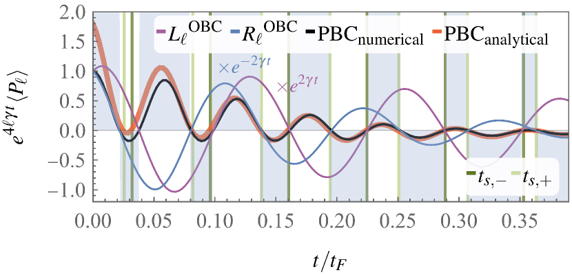
Figure 17: Directional pumping of subsystem parity for a quench to the topological PT-symmetric phase with $\alpha=2.5$, $\mu=-0.5J$, $\gamma=0.3J$, $\delta=0$, and $\ell=20$. For PBC, the subsystem parity (black line) crosses zero at multiples of both $t_{s,+}$ (light green) and $t_{s,-}$ (dark green), with blue shading indicating the sign of the subsystem parity. In contrast, for OBC, zero crossings occur at multiples of $t_{s,-}$ or $t_{s,+}$ for a subsystem located at the left ($L_{\ell}$, violet line) and right end of the chain ($R_{\ell}$, blue line). Factors $e^{\pm 2\gamma t}$ compensate for additional exponential decay and growth due to edge modes. The analytical conjecture Eq. (162) agrees well with the numerics also for the long-range model after stronger initial discrepancies (red line).

A unique property of the long-range model is the existence of a finite region in the $\mu$-$\gamma$ plane which lies outside of the PT-symmetric phase but in which the PTGGE has two soft modes as shown in Figs. 18(a), (b) for $\alpha=2.5$ and (c), (d) for $\alpha=1.5$, where the boundary of the PT-symmetric phase is indicated by a black line. This finding demonstrates that directional pumping phases are in fact not bound to dynamical phases determined by PT symmetry. To understand the origin of the difference in phase boundaries, note that solutions to Eq. (182) exist for values of $\mu$ and $\gamma$ between the extrema of $J_{k}$ at $k=0,\pi$ where $J_{0}=J$ and $J_{\pi}=-J\eta(\alpha)/\zeta(\alpha)$, leading to the conditions $\left\lvert 2J_{0}+\mu\right\rvert=2\gamma$ and $\left\lvert 2J_{\pi}+\mu\right\rvert=2\gamma$ that determine the boundaries of directional pumping phases. In particular, $\omega_{k_{s,-}}$ is nonzero for $\mu_{c,<}<\mu<\mu_{c,>}$ and $\gamma<2\left(J_{0}-J_{\pi}-\left\lvert\mu-\mu_{m}\right\rvert\right)$. The PT-symmetric phase is delimited by a smaller critical value of $\gamma$ for $\mu_{b,<}<\mu<\mu_{b,>}$. Outside of that range, the phase boundaries coincide.

VIII.3.2 Dynamical criticality

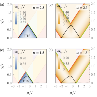
Figure 18: Directional parity pumping phase diagrams of the long-range Kitaev chain determined by the soft-mode frequencies $\omega_{k_{s,\pm}}$ for (a), (b) $\alpha=2.5$ and (c), (d) $\alpha=1.5$. Background colors indicate phases defined by PT symmetry as in Fig. 14. The boundary of the PT-symmetric topological phase is shown as a black line. Red and green lines indicate phase boundaries at which the critical exponents are and are not modified, respectively, in comparison to the short-range Kitaev chain.

The product $\nu^{\prime}z^{\prime}$ of critical exponents describes how the soft-mode time scales $t_{s,\pm}$ diverge at the boundaries of directional pumping phases. For the long-range Kitaev chain, this divergence is the same as in the short-range Kitaev chain for the phase boundaries that are shown as green lines in Fig. 18; but for the phase boundaries that are shown as red lines, long-range hopping and pairing lead to modified critical behavior. To derive the corresponding exponents, we note that according to Eq. (182), at directional pumping phase boundaries, $\left\lvert\Delta_{k_{s,\pm}}\right\rvert=\omega_{k_{s,\pm}}/2$ vanishes, which is the case for $k_{s,\pm,c}=0,\pm\pi$. We can then determine the scaling behavior of $k_{s,\pm}$ as in the short-range Kitaev chain by inserting $\mu=\mu_{c}+\delta_{\mu}$ and $\gamma=\gamma_{c}+\delta_{\gamma}$ in Eq. (182) and expanding in $k$ around $k_{s,\pm,c}=0,\pm\pi$. Modified scaling behavior of $k_{s,\pm}$ as compared to the short-range model occurs if the expansions of $J_{k}$ and $\Delta_{k}$ are modified as compared to $J\cos(k)$ and $\Delta\sin(k)$, respectively. This is the case for the expansions around $k=0$: Depending on the value of $\alpha$, different exponents dominate in Eq. (231), leading to

$$J_{k}-J_{0}\sim\begin{cases}k^{2}&\text{for }3<\alpha,\\ k^{\alpha-1}&\text{for }1<\alpha<3,\end{cases}$$ (184)

and

$$\Delta_{k}\sim\begin{cases}k&\text{for }2<\alpha,\\ k^{\alpha-1}&\text{for }1<\alpha<2.\end{cases}$$ (185)

For the phase boundaries with modified scaling behavior, which are indicated by red lines in Fig. 18, we thus find

$$\nu^{\prime} =1/2, z^{\prime} =1 3<\alpha,$$ for (186)

$$\nu^{\prime} =1/\left(\alpha-1\right), z^{\prime} =1 2<\alpha<3,$$ for

$$\nu^{\prime} =1/\left(\alpha-1\right), z^{\prime} =(\alpha-1) 1<\alpha<2.$$ for

Otherwise, when $k_{s,\pm,c}=\pm\pi$ which is the case for the phase boundaries that are shown as green lines, the leading powers in the expansions of $J_{k}$ and $\Delta_{k}$ and, therefore, the critical exponents $\nu^{\prime}$ and $z^{\prime}$ are the same as in the short-range Kitaev chain and the SSH model and given in Eq. (169).

An efficient way to probe the modified exponents numerically is to perform quenches for a range of values of $\mu$ and $\gamma$ close to a phase boundary and measure the time $t_{1}$ at which the first zero crossing of the subsystem fermion parity occurs. In Fig. 19(a), we set $\mu=\mu_{c,<}+\delta_{\mu}$ and $\gamma=0$, and we consider the fermion parity of the left half of the system $L_{L/2}=\{1,\dotsc,L/2\}$ in a chain with OBC and for different values of $\alpha$. By decreasing the value of $\delta_{\mu}$, we expect to observe a scaling behavior $t_{1}\sim\delta_{\mu}^{-\nu^{\prime}z^{\prime}}$ with exponents given in Eq. (186). Indeed, we find good agreement between the predicted exponents and the numerical data for $\alpha>2$. For $\alpha<2$, due to the limited system sizes in our simulations, we cannot fully reach the scaling regime, we still observe a clear tendency toward the analytically predicted scaling behavior. In Fig. 19(b), we present an analogous analysis for quenches to the PT-mixed phase, where we set $\mu=\mu_{c,<}$ and $\gamma=\delta_{\gamma}$. Here, pumping of fermion parity occurs only through the left end of a subsystem and, therefore, we consider a subsystem $R_{L/2}=\{L/2+1,\dotsc,L\}$ corresponding to the right half of the chain. Even though numerics in the PT-mixed phase are restricted to smaller system sizes, we again find compelling agreement with the analytical exponents for $\alpha>2$, and a clear trend toward the analytical prediction for $\alpha<2$.

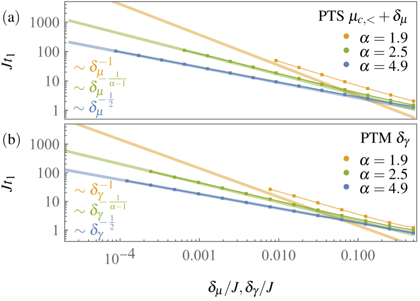
Figure 19: Scaling behavior of the first crossing time $t_{1}$ for the subsystem parity in the long-range Kitaev chain. The connected dots show numerical results for $\alpha=4.9$ (blue), $\alpha=2.5$ (green) and $\alpha=1.9$ (orange), and the expected scaling behavior according to Eq. (186) is indicated by solid lines, with scaling exponents given in the left lower corner of each panel. We consider quenches to (a) the PT-symmetric (PTS) phase with $\mu=\mu_{c,<}+\delta_{\mu}$ and $\gamma=0$, and (b) the PT-mixed (PTM) phase with $\mu=\mu_{c,<}$ and $\gamma=\delta_{\gamma}$, for a chain with OBC and subsystems located at (a) the left ($L_{\ell}$ with $\ell=L/2=500$) and (b) the right end of the chain ($R_{\ell}$ with $\ell=L/2=300$).

VIII.4 Connected density autocorrelation function

For each momentum mode $k$, the Liouvillian single-particle eigenvalues $\lambda_{\pm,k}=-i2\gamma\pm\omega_{k}$ are formally identical to the eigenfrequencies of a damped harmonic oscillator with undamped natural frequency $\varepsilon_{k}$ and damping rate $2\gamma$. When the damping rate is increased, the mode $k$ undergoes a transition from under- to overdamped oscillations—or, equivalently, from PT-symmetric to PT-breaking—when $\varepsilon_{k}=2\gamma$ in Eq. (65). It is interesting to compare how different observables are affected by this overdamping transition. The oscillation frequencies of the topological disorder parameters of the SSH model and the Kitaev chain are determined by the soft modes $k_{s,\pm}$, and directional pumping transitions occur when either of these modes becomes overdamped. According to our definition of these modes, $k_{s,-}$ is the first to become overdamped, as shown in the phase diagrams in Figs. 11, 13, and 18. But even when $k_{s,-}$ is overdamped while $k_{s,+}$ is not, for a system with PBC or a subsystem that is not on the left end of a system with OBC, the topological disorder parameters exhibit underdamped oscillatory decay as illustrated in Fig. 12. To observe this behavior, it seems to be crucial that the disorder parameters act nontrivially on sufficiently large subsystems of size $\ell$. Indeed, underdamped oscillatory decay persist until leveling, caused by the finiteness of $\ell$, sets in. As an important example of a local observable with support on only a small number of lattice sites, we consider the density autocorrelation function in the steady state of the driven-dissipative long-range Kitaev chain. As we show in the following, upon increasing the strength of dissipation $\gamma$, the decay of the density autocorrelation function becomes overdamped as soon as the first momentum mode becomes overdamped, i.e., at the transition from the PT-symmetric to the PT-broken phase. Concomitantly, one of the base oscillation periods of the density autocorrelation function diverges. However, the exponent that governs this divergence is fully determined by PT symmetry, and its value is not modified by long-range couplings.

The density autocorrelation function is defined as

$$A_{l}(t)=-4\left\langle\left(n_{l}(t)-1/2\right)\left(n_{l}(0)-1/2\right)\right\rangle_{\mathrm{SS}},$$ (187)

where $n_{l}=c_{l}^{\dagger}c_{l}$ and the normalization is chosen to obtain a simple expression in terms of Majorana fermions. We evaluate the density autocorrelation function in the steady state, which for $\gamma_{l}=\gamma_{g}$ is at infinite temperature. In Appendix E, we derive and solve the equation of motion for the density autocorrelation function. The solution can be expressed in terms of sums over contributions from momentum modes, each containing a factor $e^{-i\lambda_{\pm,k}t}$. This form immediately implies overdamped late-time decay in PT-mixed and PT-broken phases: In these phases, the dominant contribution stems from the mode with the smallest decay rate, given by $\gamma_{s}$ in Eq. (145). But this mode is nonoscillatory. In contrast, in the PT-symmetric phase, the density autocorrelation function shows oscillatory decay. As detailed in Appendix E, in the thermodynamic limit, the rescaled density autocorrelation function $e^{4\gamma t}A_{l}(t)$ can be written as a sum of squares of integrals of the form

$$I=\frac{1}{\pi}\mathop{\mathrm{Im}}\!\left(\int_{0}^{\pi}dk\,f_{k}\frac{e^{i\omega_{k}t}}{\omega_{k}}\right),$$ (188)

where $f_{k}=2J_{k}+\mu$ or $f_{k}=1$. We obtain the asymptotic behavior of the density autocorrelation function for $t\to\infty$ by evaluating these integrals in a stationary phase approximation [90]. To apply this method, we need to identify the stationary points $k_{0}$ determined by $\omega_{k}^{\prime}|_{k=k_{0}}=\varepsilon_{k}^{\prime}|_{k=k_{0}}=0$, where primes denote derivatives with respect to $k$. According to our discussion of the dispersion relation in Sec. VIII.2, the stationary points in the interval $0\leq k_{0}\leq\pi$ are given by $k_{0}\in\{0,k_{b},\pi\}$. The asymptotic behavior of the integral in Eq. (188) is determined by momenta close to the stationary points, and we obtain

$$I\sim\frac{1}{\sqrt{2\pi t}}\left(I_{s}(0)+2I_{s}(k_{b})+I_{s}(\pi)\right),$$ (189)

where the terms $I_{s}(k_{0})$ oscillate at the frequencies $\omega_{k_{0}}$,

$$I_{s}(k_{0})\sim\frac{f_{k_{0}}\sin\!\left(\omega_{k_{0}}t+\mathop{\mathrm{sgn}}\!\left(\omega^{\prime\prime}_{k_{0}}\right)\pi/4\right)}{\omega_{k_{0}}\left\lvert\omega^{\prime\prime}_{k_{0}}\right\rvert^{1/2}}.$$ (190)

For $\alpha<3$, the second derivative $\omega_{k}^{\prime\prime}$ is undefined at $k_{0}=0$, and the corresponding contribution to $I$ has to be dropped. We omit the lengthy explicit asymptotic expression for $A_{l}(t)$. But the asymptotic result for $I$ already shows that the density autocorrelation function exhibits oscillatory decay with the base frequencies $\omega_{0}$, $\omega_{k_{b}}$, and $\omega_{\pi}$.

As discussed in Sec. VIII.2, the minimum of $\varepsilon_{k}$ is at $0$, $k_{b}$, and $\pi$, for $\mu<\mu_{b,<}$, $\mu_{b,<}<\mu<\mu_{b,>}$, and $\mu_{b,>}<\mu$, respectively. Therefore, upon increasing $\gamma$, gap closings with $\omega_{k_{0}}\to 0$, which mark the transition to the PT-mixed phase, occur at these momenta, similarly to $\omega_{k_{s,\pm}}$ going to zero at directional pumping phase transitions. However, while the exponents that describe the critical behavior of $\omega_{k_{s,\pm}}$ are modified in the presence of long-range couplings as described by Eq. (186) and illustrated in Fig. 19, the base frequencies of the density autocorrelation function always vanish as a square root of the deviation $\delta_{\gamma}=\gamma-\gamma_{c}$ of the dissipation rate $\gamma$ from the critical value for the transition to the PT-mixed phase, $\omega_{k_{0}}\sim\left\lvert\delta_{\gamma}\right\rvert^{1/2}$.

The value of $1/2$ of the exponent is, in fact, determined by PT symmetry. For the Kitaev chain, the PT symmetry condition takes the same form as given in Eq. (25) for the SSH model, but for the matrix $x_{k}^{\prime}=\mathbf{x}_{k}\cdot\boldsymbol{\sigma}$ corresponding to the traceless part of the matrix $x_{k}$ defined in Appendix E, and given explicitly by $\mathbf{x}_{k}=\left(2\Delta_{k},-2J_{k}-\mu,-i2\gamma\right)$ [37]. Without resorting to the explicit form of $\mathbf{x}_{k}$ for the Kitaev chain, PTS implies that $x_{x,k},x_{y,k}\in\mathbb{R}$ whereas $x_{z,k}\in i\mathbb{R}$, such that $\omega_{k}=\sqrt{x_{x,k}^{2}+x_{y,k}^{2}-\left(ix_{z,k}\right)^{2}}$. At the transition to the PT-mixed phase, the difference under the square root vanishes for a particular momentum $k_{0}$. For the example of the Kitaev chain, $ix_{z,k}=2\gamma$, and a gap closing occurs at $\gamma=\gamma_{c}$, where $x_{x,k_{0}}^{2}+x_{y,k_{0}}^{2}-4\gamma_{c}^{2}=0$. If we now set $\gamma=\gamma_{c}+\delta_{\gamma}$ and approach the gap closing by taking the limit $\delta_{\gamma}\to 0$, we find

$$\omega_{k_{0}}=\sqrt{x_{x,k_{0}}^{2}+x_{y,k_{0}}^{2}-4\left(\gamma_{c}+\delta_{\gamma}\right)^{2}}\sim\left\lvert\delta_{\gamma}\right\rvert^{1/2},$$ (191)

in agreement with the analysis of response functions in Ref. [86]. We stress that this result follows directly from the reality conditions imposed upon $x_{x,k}$, $x_{y,k}$, and $ix_{z,k}$ by PT symmetry, and holds also for more general forms of $x_{z,k}$.

Finally, we note that for an isolated system with $x_{z,k}=0$ such that $\omega_{k}=\sqrt{x_{x,k}^{2}+x_{y,k}^{2}}$, gap closings require that $x_{x,k_{0}}=x_{y,k_{0}}=0$. Considering again the Kitaev chain with $x_{x,k}=2\Delta_{k}$ and $x_{y,k}=-2J_{k}-\mu$, gap closings occur at $k_{0}=0,\pi$ where $x_{x,k_{0}}=2\Delta_{k_{0}}=0$. Then, with $\mu=\mu_{c,\lessgtr}+\delta_{\mu}$, we obtain $\omega_{k_{0}}\sim\left\lvert\delta_{\mu}\right\rvert$. In contrast, the soft-mode frequencies vanish for $\gamma=0$ as $\omega_{k_{s,\pm}}\sim\left\lvert\delta_{\mu}\right\rvert^{1/2}$, which provides further evidence for the independence of dynamical criticality at the boundaries of directional pumping phases.

IX Conclusions and outlook

Through the study of quantum quenches in driven-dissipative many-body systems, our work determines PT symmetry as the principal driver of local relaxation to a PT-symmetric generalized Gibbs ensemble for two fundamental classes of quadratic fermionic models. In this way, we substantially extend the field of quantum quenches and relaxation of many-body systems by establishing local equilibration also for open systems with finite coupling to external reservoirs.

We have presented the theoretical framework of the PTGGE for driven-dissipative versions of the SSH model and the Kitaev chain, which can be regarded as natural open-system generalizations of paradigmatic examples of one-dimensional topological insulators and superconductors. These models differ by the presence of a weak $\mathrm{U}(1)$ symmetry [72], which leads to the vanishing of anomalous correlations in the open SSH model, even though the coupling to reservoirs breaks particle number conservation. Our analysis shows that PT symmetry of the quadratic Liouvillian is the fundamental property leading to coherent local relaxation in the presence of temporally uniform and spatially global exponential decay.

After rescaling observables to compensate this exponential decay, key features of the quench dynamics of isolated systems are revealed to persist in the PT-symmetric phase. This includes the light cone spreading of correlations and the linear-growth and volume-law saturation of the contribution to the subsystem entropy due to the propagation of pairs of entangled quasiparticles—however, with modified quasiparticle dynamics and statistics. Based on a dissipative quasiparticle picture [38, 39, 40], we have proposed an analytical conjecture for the time evolution of the quasiparticle-pair contribution to the subsystem entropy in the space-time scaling limit, which is in excellent agreement with our numerical results.

Furthermore, we have provided a detailed analysis of the dynamics of topological disorder parameters—the dual string order parameter and the subsystem fermion parity for the SSH model and the Kitaev chain, respectively. In the isolated versions of these models, the topological disorder parameters show oscillatory decay for quenches from the trivial to the topological phase. This pumping phenomenon becomes directional in driven-dissipative systems, i.e., the pumping of string order and fermion parity happens at different rates through the left and right ends of a subsystem. The pumping rates are determined by soft modes of the PTGGE, and based on this insight, we have formulated analytical conjectures for the time evolution of the topological disorder parameters, which we have found to match numerical simulations very well. Interestingly, there are parameter regimes in which there is pumping through only one end of a subsystem. This has led us to introduce the notion of directional pumping phases. As we have demonstrated using the example of a Kitaev chain with long-range hopping and pairing, directional pumping phases do, in general, not coincide with the phases determined by the breaking of PT symmetry. Moreover, we have identified a distinct form of dynamical criticality at the transitions between directional pumping phases, and we have shown that the critical exponents that govern the divergences of pumping rates are modified when the effective long-wavelength description is modified due to the presence of long-range couplings.

Our work opens up interesting prospects for future research. An important next step is to establish the generality of our results, in particular, of relaxation to the PTGGE. Our reasoning leading to the PTGGE applies to all fermionic many-body systems described by a quadratic Liouvillian with a fully PT-symmetric phase, and can be extended straightforwardly to more general quench protocols, such as for systems prepared in excited or mixed states; and we have presented first results for generalizations of the PTGGE to quadratic bosonic systems and to noninteracting fermionic systems with quadratic Hermitian jump operators in Ref. [37]. However, it remains to be seen whether relaxation to a suitably defined PTGGE occurs more generally in PT-symmetric integrable driven-dissipative systems [129, 130, 55, 131, 132, 133, 134, 135, 136, 137, 138, 139, 140, 65].

Furthermore, a possible topological origin of the zero crossings of the topological disorder parameters that occur after quenches to the gapless PT-mixed phase warrants further investigation. In Ref. [86], zero crossings of the subsystem parity were studied in a Kitaev chain with OBC and for a subsystems given by the left half of the chain. Then, crossings occur only within the gapped fully PT-symmetric phase, and have been attributed to the nontrivial non-Hermitian topology of the postquench Liouvillian. Our finding, that zero crossings occur for a subsystem at the right end of a chain with OBC and or in a chain with PBC also within the PT-mixed phase, raises the question whether the dynamical entanglement-spectrum bulk-boundary correspondence [4, 141, 108] can be extended to such phases and how it can be refined to distinguish between left and right entanglement cuts.

In addition to topological disorder parameter pumping or, equivalently, entanglement spectrum crossings, nonanalyticities of the Loschmidt echo, which have been dubbed dynamical quantum phase transitions [8, 142], have also been proposed as a dynamical signature of topology [6]. Indeed, for the isolated Kitaev chain, the soft-mode period $t_{s}$ coincides with the period of singularities of the Loschmidt echo. It will be interesting to see whether a suitable generalization of the Loschmidt echo to open systems [143, 144, 145] can capture the existence of two distinct soft-mode periods $t_{s,+}\neq t_{s,-}$ in the driven-dissipative Kitaev chain.

Appendix A Time evolution of the covariance matrix

In this appendix, we derive and solve the equation of motion of the covariance matrix for time evolution generated by a quadratic Liouvillian. We consider models with and without a weak $\mathrm{U}(1)$ symmetry, such that the state of the system is described by a covariance matrix of the form given in Eq. (6) for complex Dirac fermions and Eq. (64) for Majorana fermions, respectively. Representative examples are provided by the driven-dissipative SSH model and the Kitaev chain considered in the main text. In both cases, the covariance matrix takes the general form

$$\langle O(t)\rangle=\mathop{\mathrm{tr}}\!\left(O\rho(t)\right)=\mathop{\mathrm{tr}}\!\left(Oe^{-i\mathcal{L}t}\rho_{0}\right)=\mathop{\mathrm{tr}}\!\left(e^{i\mathcal{L}^{\dagger}t}(O)\rho_{0}\right),$$ (192)

where $O$ is quadratic in fermionic operators, and Hermitian conjugation of the Liouvillian $\mathcal{L}$ is defined with respect to the Hilbert-Schmidt inner product of operators, $\langle A,B\rangle_{\mathrm{HS}}=\mathop{\mathrm{tr}}\!\left(A^{\dagger}B\right)$. That is, the defining relation for $\mathcal{L}^{\dagger}$ reads $\langle A,\mathcal{L}B\rangle_{\mathrm{HS}}=\langle\mathcal{L}^{\dagger}A,B\rangle_{\mathrm{HS}}$. As stated in Eq. (90), we find $\mathcal{L}^{\dagger}=\mathcal{H}-i\mathcal{D}^{\dagger}$, where we have used that $\mathcal{H}=\mathcal{H}^{\dagger}$; the adjoint dissipator $\mathcal{D}^{\dagger}$ is given in Eq. (91). By taking the derivative of Eq. (192) with respect to time,

$$\frac{d}{dt}\langle O(t)\rangle=i\mathop{\mathrm{tr}}\!\left(e^{i\mathcal{L}^{\dagger}t}\left(\mathcal{L}^{\dagger}(O)\right)\rho_{0}\right)=i\langle(\mathcal{L}^{\dagger}O)(t)\rangle,$$ (193)

we see that in order to obtain the evolution equations for the covariance matrices in Eqs. (6) and (64), we have to identify the relevant operator $O$ and apply $\mathcal{L}^{\dagger}$ to this operator.

A.1 Complex Dirac fermions

We first consider a quadratic particle-number conserving Hamiltonian, defined in terms of $2L$ complex fermionic annihilation and creation operators $c_{l}$ and $c_{l}^{\dagger}$, respectively,

$$H=\sum_{l,l^{\prime}=1}^{2L}c_{l}^{\dagger}H_{l,l^{\prime}}c_{l^{\prime}}.$$ (194)

The Hamiltonian of the SSH model in Eq. (4) is obtained as a special case of this general form. Further, we consider linear jump operators that describe particle loss and gain as in Eq. (11), with bath matrices given in Eq. (12).

A.1.1 Equation of motion of the covariance matrix

To derive the equation of motion of the covariance matrix, it is convenient to consider the single-particle density matrix defined by (note the order of indices in the definition of $Q_{l,l^{\prime}}$)

$$C_{l,l^{\prime}}(t)=\langle Q_{l,l^{\prime}}(t)\rangle,\qquad Q_{l,l^{\prime}}=c_{l^{\prime}}^{\dagger}c_{l},$$ (195)

as an auxiliary quantity, which is related to the covariance matrix by $G=\mathbbm{1}-2C$. According to the discussion above, we can obtain the equation of motion of the single-particle density matrix by applying $\mathcal{L}^{\dagger}$ to $Q_{l,l^{\prime}}$. To that end, it is convenient to introduce the notation

$$Q_{l,l^{\prime}}=c_{l^{\prime}}^{\dagger}c_{l}=\sum_{m,m^{\prime}=1}^{2L}c_{m}^{\dagger}P^{l^{\prime},l}_{m,m^{\prime}}c_{m^{\prime}},\quad P^{l^{\prime},l}_{m,m^{\prime}}=\delta_{m,l^{\prime}}\delta_{m^{\prime},l}.$$ (196)

The action of the Hamiltonian $\mathcal{H}$ is then given by

$$\mathcal{H}Q_{l,l^{\prime}}=[H,Q_{l,l^{\prime}}]=\sum_{m,m^{\prime}=1}^{2L}[H,P^{l^{\prime},l}]_{m,m^{\prime}}Q_{m^{\prime},m},$$ (197)

and the contribution from the adjoint dissipator $\mathcal{D}^{\dagger}$ for arbitrary loss and gain coefficients reads

$$\mathcal{D}^{\dagger}Q_{l,l^{\prime}}=-\sum_{m,m^{\prime}=1}^{2L}\{M_{l}+M_{g},P^{l^{\prime},l}\}_{m,m^{\prime}}Q_{m^{\prime},m}+2M_{g,l,l^{\prime}}.$$ (198)

Combining Eqs. (197) and (198), we obtain

$$\mathcal{L}^{\dagger}Q_{l,l^{\prime}}=-\sum_{m,m^{\prime}=1}^{2L}\left(P^{l^{\prime},l}Z-Z^{\dagger}P^{l^{\prime},l}\right)_{m,m^{\prime}}Q_{m^{\prime},m}-i2M_{g,l,l^{\prime}},$$ (199)

where the matrix $Z$ is defined in Eq. (14), and we have used that the bath matrices defined in Eq. (12) are Hermitian. By inserting Eq. (199) in Eq. (193), and using relations such as

$$\sum_{m,m^{\prime}=1}^{2L}\left(P^{l^{\prime},l}Z\right)_{m,m^{\prime}}\mathop{\mathrm{tr}}(Q_{m^{\prime},m}\rho)=\mathop{\mathrm{tr}}\!\left(P^{l^{\prime},l}ZC\right)=\left(ZC\right)_{l,l^{\prime}},$$ (200)

where the trace on the left-hand side and after the first equality applies to operators and matrices, respectively, we obtain

$$\frac{dC}{dt}=-i\left(ZC-CZ^{\dagger}\right)+2M_{g},$$ (201)

which immediately leads to the equation of motion of the covariance matrix given in Eq. (13).

A.1.2 Formal solution of the equation of motion

To find the solution of Eq. (13), we employ the following ansatz [146]:

$$G(t)=Q(t)G_{0}Q(t)^{\dagger}-iP(t)Q(t)^{\dagger},$$ (202)

where initial conditions are given by $G_{0}=G(0)$, $Q(0)=\mathbbm{1}$ and $P(0)=0$. This ansatz satisfies Eq. (13) if

$$\frac{dQ}{dt}=-iZQ,\quad\frac{dP}{dt}=-iZP+i2\left(M_{l}-M_{g}\right)Q^{-\dagger}.$$ (203)

The solutions to these equations read $Q(t)=e^{-iZt}$ and

$$P(t)=i2Q(t)\int_{0}^{t}dt^{\prime}\,Q(t^{\prime})^{-1}\left(M_{l}-M_{g}\right)Q(t^{\prime})^{-\dagger}.$$ (204)

To perform the integration over time, we express the matrix $Z$ as $Z=V\Lambda V^{-1}$, where $\Lambda$ is a diagonal matrix with entries $\lambda_{l}$. For the last term in Eq. (202), $R(t)=-iP(t)Q(t)^{\dagger}$, we find

$$R_{l,l^{\prime}}(t)=-i2V\left[\left(V^{-1}\left(M_{l}-M_{g}\right)V^{-\dagger}\right)\circ K(t)\right]V^{\dagger},$$ (205)

where

$$K_{l,l^{\prime}}(t)=\frac{1-e^{-i\left(\lambda_{l}-\lambda_{l^{\prime}}^{*}\right)t}}{\lambda_{l}-\lambda_{l^{\prime}}^{*}},$$ (206)

and where $A\circ B$ denotes the Hadamard product, i.e., the element-wise product given by $\left(A\circ B\right)_{l,l^{\prime}}=A_{l,l^{\prime}}B_{l,l^{\prime}}$. The above form of $R(t)$ is particularly convenient to evaluate the covariance matrix numerically.

A.2 Majorana fermions

Next, we consider a quadratic Hamiltonian for $2L$ Majorana fermions,

$$H=\frac{i}{4}\sum_{l,l^{\prime}=1}^{2L}w_{l}A_{l,l^{\prime}}w_{l^{\prime}},$$ (207)

where without loss of generality we assume that $A$ is antisymmetric, $A=-A^{{\mathchoice{\raisebox{0.0pt}{$\displaystyle\intercal$}}{\raisebox{0.0pt}{$\textstyle\intercal$}}{\raisebox{0.0pt}{$\scriptstyle\intercal$}}{\raisebox{0.0pt}{$\scriptscriptstyle\intercal$}}}}$. The representation of the Hamiltonian of the Kitaev chain Eq. (60) in this form is provided in Ref. [37]. We further consider linear jump operators and define the bath matrix $M$ through

$$L_{l}=\sum_{l,l^{\prime}=1}^{2L}B_{l,l^{\prime}}w_{l^{\prime}},\qquad M=B^{{\mathchoice{\raisebox{0.0pt}{$\displaystyle\intercal$}}{\raisebox{0.0pt}{$\textstyle\intercal$}}{\raisebox{0.0pt}{$\scriptstyle\intercal$}}{\raisebox{0.0pt}{$\scriptscriptstyle\intercal$}}}}B^{*},$$ (208)

which includes Eq. (61) as a special case.

A.2.1 Equation of motion of the covariance matrix

In analogy to Eq. (195), we define a single-particle density matrix for Majorana fermions,

$$\Xi_{l,l^{\prime}}(t)=i\langle W_{l,l^{\prime}}(t)\rangle,\qquad W_{l,l^{\prime}}=w_{l}w_{l^{\prime}},$$ (209)

such that the covariance matrix in Eq. (64) is given by $\Gamma=\Xi-i\mathbbm{1}$. To calculate the action of $\mathcal{L}^{\dagger}$ on $W_{l,l^{\prime}}$ and thus obtain the equation of motion of the single-particle density matrix, we write $W_{l,l^{\prime}}$ as

$$W_{l,l^{\prime}}=w_{l}w_{l^{\prime}}=\sum_{m,m^{\prime}=1}^{2L}w_{m}P^{l,l^{\prime}}_{m,m^{\prime}}w_{m^{\prime}},\quad P^{l,l^{\prime}}_{m,m^{\prime}}=\delta_{m,l}\delta_{m^{\prime},l^{\prime}}.$$ (210)

The Hamiltonian contribution to $\mathcal{L}^{\dagger}W_{l,l^{\prime}}$ is given by

$$\mathcal{H}W_{l,l^{\prime}}=[H,W_{l,l^{\prime}}]=i\sum_{m,m^{\prime}=1}^{2L}[A,P^{l^{\prime},l}]_{m,m^{\prime}}W_{m^{\prime},m}.$$ (211)

Next, we calculate the action of the dissipator on $W_{l,l^{\prime}}$:

$$\mathcal{D}^{\dagger}W_{l,l^{\prime}}=-4\sum_{m,m^{\prime}=1}^{2L}\{M_{R},P^{l^{\prime},l}\}_{m,m^{\prime}}W_{m^{\prime},m}+8M_{l,l^{\prime}}^{{\mathchoice{\raisebox{0.0pt}{$\displaystyle\intercal$}}{\raisebox{0.0pt}{$\textstyle\intercal$}}{\raisebox{0.0pt}{$\scriptstyle\intercal$}}{\raisebox{0.0pt}{$\scriptscriptstyle\intercal$}}}},$$ (212)

where we have used that the real part $M_{R}=\mathop{\mathrm{Re}}(M)$ and the imaginary part $M_{I}=\mathop{\mathrm{Im}}(M)$ of the bath matrix are symmetric and antisymmetric, respectively. Combining Eqs. (211) and (212) we obtain

$$\mathcal{L}^{\dagger}W_{l,l^{\prime}}=i\sum_{m,m^{\prime}=1}^{2L}\left(X^{{\mathchoice{\raisebox{0.0pt}{$\displaystyle\intercal$}}{\raisebox{0.0pt}{$\textstyle\intercal$}}{\raisebox{0.0pt}{$\scriptstyle\intercal$}}{\raisebox{0.0pt}{$\scriptscriptstyle\intercal$}}}}P^{l^{\prime},l}+P^{l^{\prime},l}X\right)_{m,m^{\prime}}W_{m^{\prime},m}-i8M_{l,l^{\prime}}^{{\mathchoice{\raisebox{0.0pt}{$\displaystyle\intercal$}}{\raisebox{0.0pt}{$\textstyle\intercal$}}{\raisebox{0.0pt}{$\scriptstyle\intercal$}}{\raisebox{0.0pt}{$\scriptscriptstyle\intercal$}}}}$$ (213)

where

$$X=-A+4M_{R}.$$ (214)

We obtain the equation of motion for the single-particle density matrix by inserting Eq. (213) in Eq. (193), which then leads to the equation of motion for the covariance matrix,

$$\frac{d\Gamma}{dt}=-X\Gamma-\Gamma X^{{\mathchoice{\raisebox{0.0pt}{$\displaystyle\intercal$}}{\raisebox{0.0pt}{$\textstyle\intercal$}}{\raisebox{0.0pt}{$\scriptstyle\intercal$}}{\raisebox{0.0pt}{$\scriptscriptstyle\intercal$}}}}-Y,$$ (215)

where $Y=-8M_{I}$.

A.2.2 Formal solution of the equation of motion

For the sake of completeness, we note that the formal solution of Eq. (215) reads

$$\Gamma(t)=e^{-Xt}\Gamma(0)e^{-X^{{\mathchoice{\raisebox{0.0pt}{$\displaystyle\intercal$}}{\raisebox{0.0pt}{$\textstyle\intercal$}}{\raisebox{0.0pt}{$\scriptstyle\intercal$}}{\raisebox{0.0pt}{$\scriptscriptstyle\intercal$}}}}t}-\int_{0}^{t}dt^{\prime}\,e^{-X\left(t-t^{\prime}\right)}Ye^{-X^{{\mathchoice{\raisebox{0.0pt}{$\displaystyle\intercal$}}{\raisebox{0.0pt}{$\textstyle\intercal$}}{\raisebox{0.0pt}{$\scriptstyle\intercal$}}{\raisebox{0.0pt}{$\scriptscriptstyle\intercal$}}}}\left(t-t^{\prime}\right)}.$$ (216)

The integral over time can be performed as detailed in Ref. [37].

Appendix B Diagonalization of $z_{k}$

The non-Hermitian Bloch Hamiltonian of the driven-dissipative SSH model, $z_{k}=z_{\mathbbm{1}}\mathbbm{1}+\mathbf{z}_{k}\cdot\boldsymbol{\sigma}$ defined in Eq. (20), can be diagonalized in the PT-symmetric phase by applying two consecutive rotations by a real and an imaginary angle, respectively, as described by the nonunitary matrix

$$U_{k}=U_{z,-\phi_{k}}U_{y,-i\theta_{k}+\pi/2}=e^{-i\left(\phi_{k}/2\right)\sigma_{z}}e^{\left[\left(\theta_{k}-i\pi/2\right)/2\right]\sigma_{y}},$$ (217)

where the angles $\phi_{k}$ and $\theta_{k}$ are defined by the relations

$$\varepsilon_{k}e^{i\phi_{k}} =J_{1}+J_{2}\cos(k)+iJ_{2}\sin(k),$$ (218)

$$\theta_{k} =\mathop{\mathrm{acosh}}\!\left(\frac{\varepsilon_{k}}{\omega_{k}}\right)=\mathop{\mathrm{asinh}}\!\left(\frac{2\Delta\gamma}{\omega_{k}}\right).$$ (219)

This leads to the following representation of $z_{k}$:

$$z_{k}=z_{\mathbbm{1}}\mathbbm{1}+\omega_{k}U_{k}\sigma_{z}U_{k}^{-1},$$ (220)

with the dispersion relation of the driven-dissipative SSH model $\omega_{k}$ given in Eq. (33). For the isolated SSH model with $\Delta\gamma=0$, the above relation reduces to Eq. (27).

Appendix C Proof of Eq. (159)

As explained in Sec. III.1, due to the weak $\mathrm{U}(1)$ symmetry of the driven-dissipative SSH model, if there are no anomalous correlations in the initial state, no such correlations will be generated in the dynamics, and, therefore, the state of the system is at all times fully determined by the covariance matrix defined in Eq. (6). Consequently, describing the state in terms of a covariance matrix for Majorana fermions appears to be unnatural and inefficient. However, as stated in Eq. (156), the dual string order parameter has a simple representation in terms of Majorana fermions, which, by applying Wick’s theorem, immediately leads to the expression Eq. (157) for the expectation value of the dual string order parameter as the Pfaffian of a submatrix $\Gamma_{\ell}$ of the Majorana covariance matrix. In this appendix, we provide a proof for Eq. (159) which relates $\Gamma_{\ell}$ to the reduced covariance matrix $G_{1,\ell}$ defined in terms of complex fermions—confirming that there is no information in $\Gamma_{\ell}$ that is not already contained in $G_{1,\ell}$. For simplicity, we consider a translationally invariant state of a system with PBC, but these assumptions are not crucial.

We begin by defining a complex covariance matrix that includes anomalous correlations $\langle c_{l}c_{l^{\prime}}\rangle$ and $\langle c_{l}^{\dagger}c_{l^{\prime}}^{\dagger}\rangle$, even though these vanish for the SSH model:

$$F_{l,l^{\prime}}=\left\langle\left[C_{l},C_{l^{\prime}}^{\dagger}\right]\right\rangle,$$ (221)

with $C=\left(c_{1},c_{1}^{\dagger},\dotsc,c_{2L},c_{2L}^{\dagger}\right)^{{\mathchoice{\raisebox{0.0pt}{$\displaystyle\intercal$}}{\raisebox{0.0pt}{$\textstyle\intercal$}}{\raisebox{0.0pt}{$\scriptstyle\intercal$}}{\raisebox{0.0pt}{$\scriptscriptstyle\intercal$}}}}$. The Majorana covariance matrix for the SSH model, introduced in Sec.VII.1, can then be written as

$$\Gamma=iR_{2L}^{\dagger}FR_{2L},$$ (222)

where the matrix converting between Majorana and complex fermions is given by

$$R_{\ell}=\bigoplus_{l=1}^{\ell}\frac{1}{\sqrt{2}}\begin{pmatrix}1&-i\\ 1&i\end{pmatrix}.$$ (223)

We want to understand the structure of the submatrix $\Gamma_{\ell}$ introduced in Eq. (158). To that end, we first consider the structure of $F$. For a translationally invariant state, $F$ can be decomposed into $4\times 4$ blocks $f_{l}$ which can be expressed in terms of the elements of the covariance matrix Eq. (6) as

$$f_{l-l^{\prime}}=\begin{pmatrix}G_{2l-1,2l^{\prime}-1}&0&G_{2l-1,2l^{\prime}}&0\\ 0&-G_{2l^{\prime}-1,2l-1}&0&-G_{2l^{\prime},2l-1}\\ G_{2l,2l^{\prime}-1}&0&G_{2l,2l^{\prime}}&0\\ 0&-G_{2l^{\prime}-1,2l}&0&-G_{2l^{\prime},2l}\end{pmatrix},$$ (224)

where the zero entries are due to the vanishing of anomalous correlations. Next, we consider the transformation to Majorana fermions in Eq. (222). For a $4\times 4$ block $\gamma_{l}$ of $\Gamma$, we obtain

$$\gamma_{l}=iR_{2}^{\dagger}f_{l}R_{2}.$$ (225)

To calculate the dual string order parameter according to Eq. (157), we require not the full matrix $\Gamma$ but rather the submatrix $\Gamma_{\ell}$ specified in Eq. (158). This submatrix is composed of $2\times 2$ blocks $\left(\gamma_{\ell}\right)_{l}$ that are cut out from the center of the $4\times 4$ blocks $\gamma_{l}$ and given by

$$\left(\gamma_{\ell}\right)_{l-l^{\prime}}\\ =\frac{1}{2}\begin{pmatrix}i\left(G_{2l-1,2l^{\prime}-1}-G_{2l^{\prime}-1,2l-1}\right)&-\left(G_{2l-1,2l^{\prime}}+G_{2l^{\prime},2l-1}\right)\\ G_{2l,2l^{\prime}-1}+G_{2l^{\prime}-1,2l}&i\left(G_{2l,2l^{\prime}}-G_{2l^{\prime},2l}\right)\end{pmatrix}.$$ (226)

When we decompose the covariance matrix as $G=G_{1}+G_{2}$ in analogy to Eq. (48), a drastic simplification of $\left(\gamma_{\ell}\right)_{l}$ results from the symmetry properties of $G_{1}$ and $G_{2}$ stated in Eq. (59). In particular, we find that the contribution due to $G_{2}$ drops out,

$$\left(\gamma_{\ell}\right)_{l-l^{\prime}}=\begin{pmatrix}iG_{1,2l-1,2l^{\prime}-1}&-G_{1,2l-1,2l^{\prime}}\\ G_{1,2l,2l^{\prime}-1}&iG_{1,2l,2l^{\prime}}\end{pmatrix}.$$ (227)

Comparing this to the block structure of $G$ given by

$$g_{1,l-l^{\prime}}=\begin{pmatrix}G_{1,2l-1,2l^{\prime}-1}&G_{1,2l-1,2l^{\prime}}\\ G_{1,2l,2l^{\prime}-1}&G_{1,2l,2l^{\prime}}\end{pmatrix},$$ (228)

we find that

$$\left(\gamma_{\ell}\right)_{l}=iP_{1}^{\dagger}g_{1,l}P_{1},$$ (229)

where $P_{\ell}$ is defined in Eq. (160). For the full matrices $\Gamma_{\ell}$ and $G_{1,\ell}$, this relation leads to Eq. (159).

Appendix D Polylogarithm and Riemann zeta function

The polylogarithm and the Riemann zeta function are defined as [147]

$$\mathrm{Li}_{\alpha}(z)=\sum_{n=1}^{\infty}\frac{z^{n}}{n^{\alpha}},\qquad\zeta(\alpha)=\sum_{n=1}^{\infty}\frac{1}{n^{\alpha}}=\mathrm{Li}_{\alpha}(1).$$ (230)

To make analytical progress when working with the polylogarithm, we employ the series expansions of $\mathrm{Li}_{\alpha}\!\left(e^{ik}\right)$ around $k=0$ and $k=\pi$. The expansion around $k=0$ reads [147]

$$\mathrm{Li}_{\alpha}\!\left(e^{ik}\right)=\Gamma\!\left(1-\alpha\right)\left(-ik\right)^{\alpha-1}+\sum_{n=0}^{\infty}\frac{\zeta\!\left(\alpha-n\right)}{n!}\left(ik\right)^{n},$$ (231)

which holds for $\left\lvert k\right\rvert<2\pi$ and $\alpha\notin\mathbb{N}$, and where $\Gamma(\alpha)$ is the gamma function. For $\alpha\in\mathbb{N}$, the expansion is given by [148]

$$\mathrm{Li}_{\alpha}\!\left(e^{ik}\right)=\frac{\left(ik\right)^{\alpha-1}}{\left(\alpha-1\right)!}\left(H_{\alpha-1}-\log\!\left(-ik\right)\right)+\sum_{\begin{subarray}{c}n=0\\ n\neq\alpha-1\end{subarray}}^{\infty}\frac{\zeta\!\left(\alpha-n\right)}{n!}\left(ik\right)^{n},$$ (232)

where $H_{\alpha}=\sum_{n=1}^{\alpha}\frac{1}{n}$ is the $\alpha$-th harmonic number with $H_{0}=0$. The expansion of the polylogarithm around $k=\pi$ reads

$$\mathrm{Li}_{\alpha}\!\left(e^{ik}\right)=-\sum_{n=0}^{\infty}\frac{\eta\!\left(\alpha-n\right)}{n!}\left[i\left(k-\pi\right)\right]^{n},$$ (233)

where $\eta(\alpha)=\left(1-2^{1-\alpha}\right)\zeta(\alpha)$ is the Drichlet eta function.

Appendix E Density autocorrelation function

The connected density autocorrelation function defined in Eq. (187) can be regarded as a special case of the Majorana four-point function

$$B_{l_{1},l_{2},l_{3}}(t)=\langle W_{l_{1},l_{2}}(t)W_{2l_{3}-1,2l_{3}}(0)\rangle_{\mathrm{SS}},$$ (234)

where $W_{l,l^{\prime}}$ is given in Eq. (210) and, for $\gamma_{l}=\gamma_{g}$, the expectation value in the steady state reduces to taking the trace, $\langle\dots\rangle_{\mathrm{SS}}=\mathop{\mathrm{tr}}(\dotsb)/2^{L}$. Note that $l_{1},l_{2}\in\{1,\dotsc,2L\}$ label Majorana modes whereas $l_{3}\in\{1,\dotsc,L\}$ is a lattice-site index. The relation $W_{2l-1,2l}=i2\left(n_{l}-1/2\right)$ leads to

$$A_{l}(t)=\langle W_{2l-1,2l}(t)W_{2l-1,2l}\rangle_{\mathrm{SS}}=B_{2l-1,2l,l}(t).$$ (235)

As we show in the following, a closed equation of motion can be obtained for four-point functions of the general type given in Eq. (234). Solving this equation yields the full time dependence of the density autocorrelation function.

According to the quantum regression theorem, the two-time average in Eq. (234) can be calculated as [149]

$$\begin{split}B_{l_{1},l_{2},l_{3}}(t)&=\mathop{\mathrm{tr}}\!\left(W_{l_{1},l_{2}}e^{-i\mathcal{L}t}(W_{2l_{3}-1,2l_{3}}\rho_{\mathrm{SS}})\right)\\ &=\mathop{\mathrm{tr}}\!\left(e^{i\mathcal{L}^{\dagger}}(W_{l_{1},l_{2}})W_{2l_{3}-1,2l_{3}}\rho_{\mathrm{SS}}\right),\end{split}$$ (236)

where the adjoint Liouvillian is defined in Eq. (90). By taking the derivative with respect to time, we obtain

$$\frac{dB_{l_{1},l_{2},l_{3}}}{dt}=i\mathop{\mathrm{tr}}\!\left(\mathcal{L}^{\dagger}(W_{l_{1},l_{2}})e^{-i\mathcal{L}t}(W_{2l_{3}-1,2l_{3}}\rho_{\mathrm{SS}})\right),$$ (237)

and inserting here Eq. (213) leads to

$$\frac{dB_{l_{1},l_{2},l_{3}}}{dt}=-\sum_{m=1}^{2L}\left(X_{l_{1},m}B_{m,l_{2},l_{3}}+B_{l_{1},m,l_{3}}X^{{\mathchoice{\raisebox{0.0pt}{$\displaystyle\intercal$}}{\raisebox{0.0pt}{$\textstyle\intercal$}}{\raisebox{0.0pt}{$\scriptstyle\intercal$}}{\raisebox{0.0pt}{$\scriptscriptstyle\intercal$}}}}_{m,l_{2}}\right).$$ (238)

In the last term, we have used $\langle W_{2l_{3}-1,2l_{3}}\rangle_{\mathrm{SS}}=i2\langle n_{l_{3}}-1/2\rangle_{\mathrm{SS}}=0$. Let us now consider a system with PBC and exploit translational invariance to represent $B_{l_{1},l_{2},l_{3}}(t)$ in terms of $2\times 2$ blocks,

$$b_{l_{1}-l_{3},l_{2}-l_{3}}=\begin{pmatrix}B_{2l_{1}-1,2l_{2}-1,l_{3}}&B_{2l_{1}-1,2l_{2},l_{3}}\\ B_{2l_{1},2l_{2}-1,l_{3}}&B_{2l_{1},2l_{2},l_{3}}\end{pmatrix},$$ (239)

that depend only on relative coordinates. Indeed, note that here all three of $l_{1},l_{2},l_{3}\in\{1,\dotsc,L\}$ are lattice-site indices. Similarly, we introduce $2\times 2$ blocks of the matrix $X$. Rewritten in terms of block matrices, the equation of motion reads

$$\frac{db_{l,l^{\prime}}}{dt}=-\sum_{m=1}^{L}\left(x_{l-m}b_{m,l^{\prime}}+b_{l,m}x_{l^{\prime}-m}^{{\mathchoice{\raisebox{0.0pt}{$\displaystyle\intercal$}}{\raisebox{0.0pt}{$\textstyle\intercal$}}{\raisebox{0.0pt}{$\scriptstyle\intercal$}}{\raisebox{0.0pt}{$\scriptscriptstyle\intercal$}}}}\right).$$ (240)

This equation can be solved straightforwardly in momentum space. To this end, we introduce the discrete Fourier transforms of the block matrices,

$$b_{k,k^{\prime}}=-i\sum_{l,l^{\prime}=1}^{L}e^{-i\left(kl+k^{\prime}l^{\prime}\right)}b_{l,l^{\prime}},\quad x_{k}=-i\sum_{l=1}^{L}e^{-ikl}x_{l},$$ (241)

in terms of which Eq. (240) can be recast as

$$\frac{db_{k,k^{\prime}}}{dt}=-i\left(x_{k}b_{k,k^{\prime}}+b_{k,k^{\prime}}x_{k^{\prime}}^{\mathchoice{\raisebox{0.0pt}{$\displaystyle\intercal$}}{\raisebox{0.0pt}{$\textstyle\intercal$}}{\raisebox{0.0pt}{$\scriptstyle\intercal$}}{\raisebox{0.0pt}{$\scriptscriptstyle\intercal$}}}\right).$$ (242)

This equation of motion is solved by

$$b_{k,k^{\prime}}(t)=e^{-ix_{k}t}b_{k,k^{\prime}}(0)e^{-ix_{k^{\prime}}^{\mathchoice{\raisebox{0.0pt}{$\displaystyle\intercal$}}{\raisebox{0.0pt}{$\textstyle\intercal$}}{\raisebox{0.0pt}{$\scriptstyle\intercal$}}{\raisebox{0.0pt}{$\scriptscriptstyle\intercal$}}}t},$$ (243)

where the initial condition $b_{k,k^{\prime}}(0)$ in momentum space can be obtained by taking the discrete Fourier transform of $b_{l,l^{\prime}}(0)=-i\sigma_{y}\delta_{l,0}\delta_{l^{\prime},0}$, leading to $b_{k,k^{\prime}}(0)=-\sigma_{y}$. In the PT-symmetric phase, where $\omega_{k}\in\mathbb{R}_{>0}$ for all $k\in\mathrm{BZ}$, we find

$$b_{k,k^{\prime}}^{1,2}(t)=-ie^{-4\gamma t}\left[a_{k}(t)a_{k^{\prime}}(t)^{*}+\left(\cos\!\left(\omega_{k}t\right)-\frac{2\gamma}{\omega_{k}}\sin\!\left(\omega_{k}t\right)\right)\right.\\ \left.\times\left(\cos\!\left(\omega_{k^{\prime}}t\right)+\frac{2\gamma}{\omega_{k^{\prime}}}\sin\!\left(\omega_{k^{\prime}}t\right)\right)\right],$$ (244)

where $a_{k}(t)=\left(2J_{k}+\mu-i2\Delta_{k}\right)\sin(\omega_{k}t)/\omega_{k}$. Finally, we obtain the density autocorrelation function as

$$\begin{split}A_{l}(t)&=b_{0,0}^{1,2}(t)=\frac{i}{L^{2}}\sum_{k,k^{\prime}\in\mathrm{BZ}}b_{k,k^{\prime}}^{1,2}(t)\\ &=e^{-4\gamma t}\left[\left\lvert A_{1,l}(t)\right\rvert^{2}-4\gamma^{2}A_{2,l}(t)^{2}+\left(\frac{dA_{2,l}(t)}{dt}\right)^{2}\right],\end{split}$$ (245)

where

$$A_{1,l}(t)=\frac{1}{L}\sum_{k\in\mathrm{BZ}}a_{k}(t),\quad A_{2,l}(t)=\frac{1}{L}\sum_{k\in\mathrm{BZ}}\frac{\sin(\omega_{k}t)}{\omega_{k}}.$$ (246)

In the thermodynamic limit, sums over momenta are replaced by integrals over $k\in[-\pi,\pi]$. Since the range of integration is symmetric, the contribution to $a_{k}(t)$ that contains $\Delta_{k}$ and is odd in $k$ can be dropped. For $\omega_{k}\in\mathbb{R}_{>0}$, we may thus write

$$\begin{split}A_{1,l}(t)&=\frac{1}{\pi}\mathop{\mathrm{Im}}\!\left(\int_{0}^{\pi}dk\,\left(2J_{k}+\mu\right)\frac{e^{i\omega_{k}t}}{\omega_{k}}\right),\\ A_{2,l}(t)&=\frac{1}{\pi}\mathop{\mathrm{Im}}\!\left(\int_{0}^{\pi}dk\,\frac{e^{i\omega_{k}t}}{\omega_{k}}\right).\end{split}$$ (247)

The asymptotic behavior of these integrals for $t\to\infty$ can be obtained by means of a stationary phase approximation as described in Sec. VIII.4.

References

- Polkovnikov et al. [2011] A. Polkovnikov, K. Sengupta, A. Silva, and M. Vengalattore, Colloquium: Nonequilibrium dynamics of closed interacting quantum systems, Rev. Mod. Phys. 83, 863 (2011).
- Eisert et al. [2015] J. Eisert, M. Friesdorf, and C. Gogolin, Quantum many-body systems out of equilibrium, Nat. Phys. 11, 124 (2015).
- Chung et al. [2013] M.-C. Chung, Y.-H. Jhu, P. Chen, and C.-Y. Mou, Quench dynamics of topological maximally entangled states, J. Phys. Condens. Matter 25, 285601 (2013).
- Gong and Ueda [2018] Z. Gong and M. Ueda, Topological Entanglement-Spectrum Crossing in Quench Dynamics, Phys. Rev. Lett. 121, 250601 (2018).
- Yang et al. [2018] C. Yang, L. Li, and S. Chen, Dynamical topological invariant after a quantum quench, Phys. Rev. B 97, 060304 (2018).
- Vajna and Dóra [2015] S. Vajna and B. Dóra, Topological classification of dynamical phase transitions, Phys. Rev. B 91, 155127 (2015).
- Pastori et al. [2020] L. Pastori, S. Barbarino, and J. C. Budich, Signatures of topology in quantum quench dynamics and their interrelation, Phys. Rev. Res. 2, 033259 (2020).
- Heyl [2018] M. Heyl, Dynamical quantum phase transitions: a review, Reports Prog. Phys. 81, 054001 (2018).
- Budich and Heyl [2016] J. C. Budich and M. Heyl, Dynamical topological order parameters far from equilibrium, Phys. Rev. B 93, 085416 (2016).
- Jaynes [1957] E. T. Jaynes, Information Theory and Statistical Mechanics, Phys. Rev. 106, 620 (1957).
- Rigol et al. [2007] M. Rigol, V. Dunjko, V. Yurovsky, and M. Olshanii, Relaxation in a Completely Integrable Many-Body Quantum System: An Ab Initio Study of the Dynamics of the Highly Excited States of 1D Lattice Hard-Core Bosons, Phys. Rev. Lett. 98, 050405 (2007).
- Rossini et al. [2007] D. Rossini, T. Calarco, V. Giovannetti, S. Montangero, and R. Fazio, Decoherence induced by interacting quantum spin baths, Phys. Rev. A 75, 032333 (2007).
- Calabrese et al. [2011] P. Calabrese, F. H. L. Essler, and M. Fagotti, Quantum Quench in the Transverse-Field Ising Chain, Phys. Rev. Lett. 106, 227203 (2011).
- Calabrese et al. [2012a] P. Calabrese, F. H. L. Essler, and M. Fagotti, Quantum quench in the transverse field Ising chain: I. Time evolution of order parameter correlators, J. Stat. Mech. Theory Exp. 2012, P07016 (2012a).
- Calabrese et al. [2012b] P. Calabrese, F. H. L. Essler, and M. Fagotti, Quantum quenches in the transverse field Ising chain: II. Stationary state properties, J. Stat. Mech. Theory Exp. 2012, P07022 (2012b).
- Essler and Fagotti [2016] F. H. L. Essler and M. Fagotti, Quench dynamics and relaxation in isolated integrable quantum spin chains, J. Stat. Mech. Theory Exp. 2016, 064002 (2016).
- Vidmar and Rigol [2016] L. Vidmar and M. Rigol, Generalized Gibbs ensemble in integrable lattice models, J. Stat. Mech. Theory Exp. 2016, 064007 (2016).
- Calabrese and Cardy [2006] P. Calabrese and J. Cardy, Time Dependence of Correlation Functions Following a Quantum Quench, Phys. Rev. Lett. 96, 136801 (2006).
- Calabrese and Cardy [2005] P. Calabrese and J. Cardy, Evolution of entanglement entropy in one-dimensional systems, J. Stat. Mech. Theory Exp. 2005, P04010 (2005).
- Alba and Calabrese [2017] V. Alba and P. Calabrese, Entanglement and thermodynamics after a quantum quench in integrable systems, Proc. Natl. Acad. Sci. 114, 7947 (2017).
- Alba and Calabrese [2018] V. Alba and P. Calabrese, Entanglement dynamics after quantum quenches in generic integrable systems, SciPost Phys. 4, 017 (2018).
- Calabrese [2020] P. Calabrese, Entanglement spreading in non-equilibrium integrable systems, SciPost Phys. Lect. Notes 20, 20 (2020).
- Breuer and Petruccione [2007] H.-P. Breuer and F. Petruccione, The Theory of Open Quantum Systems (Oxford University Press, Oxford, 2007).
- Diehl et al. [2008] S. Diehl, A. Micheli, A. Kantian, B. Kraus, H. P. Büchler, and P. Zoller, Quantum states and phases in driven open quantum systems with cold atoms, Nat. Phys. 4, 878 (2008).
- Verstraete et al. [2009] F. Verstraete, M. M. Wolf, and J. Ignacio Cirac, Quantum computation and quantum-state engineering driven by dissipation, Nat. Phys. 5, 633 (2009).
- Eisert and Prosen [2010] J. Eisert and T. Prosen, Noise-driven quantum criticality, arXiv:1012.5013 (2010).
- Sieberer et al. [2013] L. M. Sieberer, S. D. Huber, E. Altman, and S. Diehl, Dynamical Critical Phenomena in Driven-Dissipative Systems, Phys. Rev. Lett. 110, 195301 (2013).
- Sieberer et al. [2016] L. M. Sieberer, M. Buchhold, and S. Diehl, Keldysh field theory for driven open quantum systems, Reports Prog. Phys. 79, 096001 (2016).
- Maghrebi and Gorshkov [2016] M. F. Maghrebi and A. V. Gorshkov, Nonequilibrium many-body steady states via Keldysh formalism, Phys. Rev. B 93, 014307 (2016).
- Jin et al. [2016] J. Jin, A. Biella, O. Viyuela, L. Mazza, J. Keeling, R. Fazio, and D. Rossini, Cluster Mean-Field Approach to the Steady-State Phase Diagram of Dissipative Spin Systems, Phys. Rev. X 6, 031011 (2016).
- Rota et al. [2017] R. Rota, F. Storme, N. Bartolo, R. Fazio, and C. Ciuti, Critical behavior of dissipative two-dimensional spin lattices, Phys. Rev. B 95, 134431 (2017).
- Halati et al. [2022] C.-M. Halati, A. Sheikhan, and C. Kollath, Breaking strong symmetries in dissipative quantum systems: Bosonic atoms coupled to a cavity, Phys. Rev. Res. 4, L012015 (2022).
- Lange et al. [2017] F. Lange, Z. Lenarčič, and A. Rosch, Pumping approximately integrable systems, Nat. Commun. 8, 15767 (2017).
- Lange et al. [2018] F. Lange, Z. Lenarčič, and A. Rosch, Time-dependent generalized Gibbs ensembles in open quantum systems, Phys. Rev. B 97, 165138 (2018).
- Lenarčič et al. [2018] Z. Lenarčič, F. Lange, and A. Rosch, Perturbative approach to weakly driven many-particle systems in the presence of approximate conservation laws, Phys. Rev. B 97, 024302 (2018).
- Reiter et al. [2021] F. Reiter, F. Lange, S. Jain, M. Grau, J. P. Home, and Z. Lenarčič, Engineering generalized Gibbs ensembles with trapped ions, Phys. Rev. Res. 3, 033142 (2021).
- Starchl and Sieberer [2022] E. Starchl and L. M. Sieberer, Relaxation to a Parity-Time Symmetric Generalized Gibbs Ensemble after a Quantum Quench in a Driven-Dissipative Kitaev Chain, Phys. Rev. Lett. 129, 220602 (2022).
- Alba and Carollo [2022] V. Alba and F. Carollo, Hydrodynamics of quantum entropies in Ising chains with linear dissipation, J. Phys. A Math. Theor. 55, 074002 (2022).
- Carollo and Alba [2022] F. Carollo and V. Alba, Dissipative quasiparticle picture for quadratic Markovian open quantum systems, Phys. Rev. B 105, 144305 (2022).
- Alba and Carollo [2021] V. Alba and F. Carollo, Spreading of correlations in Markovian open quantum systems, Phys. Rev. B 103, L020302 (2021).
- Bender and Boettcher [1998] C. M. Bender and S. Boettcher, Real Spectra in Non-Hermitian Hamiltonians Having Symmetry, Phys. Rev. Lett. 80, 5243 (1998).
- Bender [2007] C. M. Bender, Making sense of non-Hermitian Hamiltonians, Reports Prog. Phys. 70, 947 (2007).
- Kitaev [2001] A. Y. Kitaev, Unpaired Majorana fermions in quantum wires, Physics-Uspekhi 44, 131 (2001).
- Wang et al. [2015] X. Wang, T. Liu, Y. Xiong, and P. Tong, Spontaneous -symmetry breaking in non-Hermitian Kitaev and extended Kitaev models, Phys. Rev. A 92, 012116 (2015).
- Yuce [2016] C. Yuce, Majorana edge modes with gain and loss, Phys. Rev. A 93, 062130 (2016).
- San-Jose et al. [2016] P. San-Jose, J. Cayao, E. Prada, and R. Aguado, Majorana bound states from exceptional points in non-topological superconductors, Sci. Rep. 6, 21427 (2016).
- Zeng et al. [2016] Q.-B. Zeng, B. Zhu, S. Chen, L. You, and R. Lü, Non-Hermitian Kitaev chain with complex on-site potentials, Phys. Rev. A 94, 022119 (2016).
- Menke and Hirschmann [2017] H. Menke and M. M. Hirschmann, Topological quantum wires with balanced gain and loss, Phys. Rev. B 95, 174506 (2017).
- Klett et al. [2017] M. Klett, H. Cartarius, D. Dast, J. Main, and G. Wunner, Relation between -symmetry breaking and topologically nontrivial phases in the Su-Schrieffer-Heeger and Kitaev models, Phys. Rev. A 95, 053626 (2017).
- Kawabata et al. [2018] K. Kawabata, Y. Ashida, H. Katsura, and M. Ueda, Parity-time-symmetric topological superconductor, Phys. Rev. B 98, 085116 (2018).
- Li et al. [2020] C. Li, L. Jin, and Z. Song, Coalescing Majorana edge modes in non-Hermitian -symmetric Kitaev chain, Sci. Rep. 10, 6807 (2020).
- Agarwal and Joglekar [2021] K. S. Agarwal and Y. N. Joglekar, -symmetry breaking in a Kitaev chain with one pair of gain-loss potentials, Phys. Rev. A 104, 022218 (2021).
- Prosen [2012a] T. Prosen, -Symmetric Quantum Liouvillean Dynamics, Phys. Rev. Lett. 109, 090404 (2012a).
- Prosen [2012b] T. Prosen, Generic examples of -symmetric qubit (spin-1/2) Liouvillian dynamics, Phys. Rev. A 86, 044103 (2012b).
- Medvedyeva et al. [2016] M. V. Medvedyeva, F. H. Essler, and T. Prosen, Exact Bethe Ansatz Spectrum of a Tight-Binding Chain with Dephasing Noise, Phys. Rev. Lett. 117, 137202 (2016).
- van Caspel and Gritsev [2018] M. van Caspel and V. Gritsev, Symmetry-protected coherent relaxation of open quantum systems, Phys. Rev. A 97, 052106 (2018).
- Minganti et al. [2019] F. Minganti, A. Miranowicz, R. W. Chhajlany, and F. Nori, Quantum exceptional points of non-Hermitian Hamiltonians and Liouvillians: The effects of quantum jumps, Phys. Rev. A 100, 062131 (2019).
- Shibata and Katsura [2020] N. Shibata and H. Katsura, Quantum Ising chain with boundary dephasing, Prog. Theor. Exp. Phys. 2020, 12A108 (2020).
- Huber et al. [2020] J. Huber, P. Kirton, S. Rotter, and P. Rabl, Emergence of -symmetry breaking in open quantum systems, SciPost Phys. 9, 052 (2020).
- Huybrechts et al. [2020] D. Huybrechts, F. Minganti, F. Nori, M. Wouters, and N. Shammah, Validity of mean-field theory in a dissipative critical system: Liouvillian gap, -symmetric antigap, and permutational symmetry in the model, Phys. Rev. B 101, 214302 (2020).
- Arkhipov et al. [2020] I. I. Arkhipov, A. Miranowicz, F. Minganti, and F. Nori, Liouvillian exceptional points of any order in dissipative linear bosonic systems: Coherence functions and switching between and anti- symmetries, Phys. Rev. A 102, 033715 (2020).
- Curtis et al. [2021] J. B. Curtis, I. Boettcher, J. T. Young, M. F. Maghrebi, H. Carmichael, A. V. Gorshkov, and M. Foss-Feig, Critical theory for the breakdown of photon blockade, Phys. Rev. Research 3, 023062 (2021).
- Roccati et al. [2021] F. Roccati, S. Lorenzo, G. M. Palma, G. T. Landi, M. Brunelli, and F. Ciccarello, Quantum correlations in pt-symmetric systems, Quantum Science and Technology 6, 025005 (2021).
- Roccati et al. [2022] F. Roccati, G. M. Palma, F. Ciccarello, and F. Bagarello, Non-Hermitian Physics and Master Equations, Open Systems & Information Dynamics 29, 2250004 (2022).
- Claeys and Lamacraft [2022] P. W. Claeys and A. Lamacraft, Dissipative dynamics in open XXZ Richardson-Gaudin models, Phys. Rev. Res. 4, 013033 (2022).
- Nakanishi and Sasamoto [2022] Y. Nakanishi and T. Sasamoto, phase transition in open quantum systems with Lindblad dynamics, Phys. Rev. A 105, 022219 (2022).
- Ornigotti and Szameit [2014] M. Ornigotti and A. Szameit, Quasi -symmetry in passive photonic lattices, J. Opt. 16, 065501 (2014).
- Joglekar and Harter [2018] Y. N. Joglekar and A. K. Harter, Passive parity-time-symmetry-breaking transitions without exceptional points in dissipative photonic systems, Photonics Res. 6, A51 (2018).
- Barthel and Schollwöck [2008] T. Barthel and U. Schollwöck, Dephasing and the Steady State in Quantum Many-Particle Systems, Phys. Rev. Lett. 100, 100601 (2008).
- Su et al. [1979] W. P. Su, J. R. Schrieffer, and A. J. Heeger, Solitons in polyacetylene, Phys. Rev. Lett. 42, 1698 (1979).
- Heeger et al. [1988] A. J. Heeger, S. Kivelson, J. R. Schrieffer, and W. P. Su, Solitons in conducting polymers, Rev. Mod. Phys. 60, 781 (1988).
- Buča and Prosen [2012] B. Buča and T. Prosen, A note on symmetry reductions of the Lindblad equation: transport in constrained open spin chains, New J. Phys. 14, 073007 (2012).
- Hida [1992] K. Hida, Ground-state phase diagram of the spin- ferromagnetic-antiferromagnetic alternating Heisenberg chain with anisotropy, Phys. Rev. B 46, 8268 (1992).
- Lindblad [1976] G. Lindblad, On the generators of quantum dynamical semigroups, Commun. Math. Phys. 48, 119 (1976).
- Gorini [1976] V. Gorini, Completely positive dynamical semigroups of N-level systems, J. Math. Phys. 17, 821 (1976).
- Altland and Zirnbauer [1997] A. Altland and M. R. Zirnbauer, Nonstandard symmetry classes in mesoscopic normal-superconducting hybrid structures, Phys. Rev. B 55, 1142 (1997).
- Hasan and Kane [2010] M. Z. Hasan and C. L. Kane, Colloquium: Topological insulators, Rev. Mod. Phys. 82, 3045 (2010).
- Qi and Zhang [2011] X.-L. Qi and S.-C. Zhang, Topological insulators and superconductors, Rev. Mod. Phys. 83, 1057 (2011).
- Chiu et al. [2016] C.-K. Chiu, J. C. Teo, A. P. Schnyder, and S. Ryu, Classification of topological quantum matter with symmetries, Rev. Mod. Phys. 88, 035005 (2016).
- Surace and Tagliacozzo [2022] J. Surace and L. Tagliacozzo, Fermionic Gaussian states: an introduction to numerical approaches, SciPost Phys. Lect. Notes 54 (2022).
- Barthel and Zhang [2022] T. Barthel and Y. Zhang, Solving quasi-free and quadratic Lindblad master equations for open fermionic and bosonic systems, J. Stat. Mech. Theory Exp. 2022, 113101 (2022).
- Song et al. [2019] F. Song, S. Yao, and Z. Wang, Non-Hermitian Skin Effect and Chiral Damping in Open Quantum Systems, Phys. Rev. Lett. 123, 170401 (2019).
- Kawabata et al. [2019] K. Kawabata, K. Shiozaki, M. Ueda, and M. Sato, Symmetry and Topology in Non-Hermitian Physics, Phys. Rev. X 9, 041015 (2019).
- Prosen [2008] T. Prosen, Third quantization: a general method to solve master equations for quadratic open Fermi systems, New J. Phys. 10, 043026 (2008).
- Prosen [2010] T. Prosen, Spectral theorem for the Lindblad equation for quadratic open fermionic systems, J. Stat. Mech. Theory Exp. 2010, P07020 (2010).
- Sayyad et al. [2021] S. Sayyad, J. Yu, A. G. Grushin, and L. M. Sieberer, Entanglement spectrum crossings reveal non-Hermitian dynamical topology, Phys. Rev. Res. 3, 033022 (2021).
- van Caspel et al. [2019] M. van Caspel, S. E. T. Arze, and I. P. Castillo, Dynamical signatures of topological order in the driven-dissipative Kitaev chain, SciPost Phys. 6, 26 (2019).
- Lieu et al. [2020] S. Lieu, M. McGinley, and N. R. Cooper, Tenfold Way for Quadratic Lindbladians, Phys. Rev. Lett. 124, 040401 (2020).
- Peschel and Eisler [2009] I. Peschel and V. Eisler, Reduced density matrices and entanglement entropy in free lattice models, J. Phys. A Math. Theor. 42, 504003 (2009).
- Bender and Orszag [1999] C. M. Bender and S. A. Orszag, Advanced Mathematical Methods for Scientists and Engineers I (Springer New York, New York, NY, 1999).
- Lieb and Robinson [1972] E. H. Lieb and D. W. Robinson, The finite group velocity of quantum spin systems, Commun. Math. Phys. 28, 251 (1972).
- Bernier et al. [2018] J.-S. Bernier, R. Tan, L. Bonnes, C. Guo, D. Poletti, and C. Kollath, Light-cone and diffusive propagation of correlations in a many-body dissipative system, Phys. Rev. Lett. 120, 020401 (2018).
- Malo et al. [2018] J. Y. Malo, E. P. L. van Nieuwenburg, M. H. Fischer, and A. J. Daley, Particle statistics and lossy dynamics of ultracold atoms in optical lattices, Phys. Rev. A 97, 053614 (2018).
- Cevolani et al. [2018] L. Cevolani, J. Despres, G. Carleo, L. Tagliacozzo, and L. Sanchez-Palencia, Universal scaling laws for correlation spreading in quantum systems with short- and long-range interactions, Phys. Rev. B 98, 024302 (2018).
- Maity et al. [2020a] S. Maity, S. Bandyopadhyay, S. Bhattacharjee, and A. Dutta, Growth of mutual information in a quenched one-dimensional open quantum many-body system, Phys. Rev. B 101, 180301 (2020a).
- den Nijs and Rommelse [1989] M. den Nijs and K. Rommelse, Preroughening transitions in crystal surfaces and valence-bond phases in quantum spin chains, Phys. Rev. B 40, 4709 (1989).
- Tasaki [1991] H. Tasaki, Quantum liquid in antiferromagnetic chains: A stochastic geometric approach to the Haldane gap, Phys. Rev. Lett. 66, 798 (1991).
- Jordan and Wigner [1928] P. Jordan and E. Wigner, Über das Paulische Äquivalenzverbot, Zeitschrift für Phys. 47, 631 (1928).
- de Léséleuc et al. [2019] S. de Léséleuc, V. Lienhard, P. Scholl, D. Barredo, S. Weber, N. Lang, H. P. Büchler, T. Lahaye, and A. Browaeys, Observation of a symmetry-protected topological phase of interacting bosons with Rydberg atoms, Science 365, 775 (2019).
- Bahovadinov et al. [2019] M. S. Bahovadinov, O. Gülseren, and J. Schnack, Local entanglement and string order parameter in dimerized models, J. Phys. Condens. Matter 31, 505602 (2019).
- Takada [1992] S. Takada, Nonlocal Unitary Transformation and String Order in Heisenberg Chain with Bond Alternation, Journal of the Physical Society of Japan 61, 428 (1992).
- Lieb et al. [1961] E. Lieb, T. Schultz, and D. Mattis, Two soluble models of an antiferromagnetic chain, Ann. Phys. (N. Y). 16, 407 (1961).
- Barouch et al. [1970] E. Barouch, B. M. McCoy, and M. Dresden, Statistical Mechanics of the XY Model. I, Phys. Rev. A 2, 1075 (1970).
- Barouch and McCoy [1971a] E. Barouch and B. M. McCoy, Statistical Mechanics of the Model. II. Spin-Correlation Functions, Phys. Rev. A 3, 786 (1971a).
- Barouch and McCoy [1971b] E. Barouch and B. M. McCoy, Statistical Mechanics of the XY Model. III, Phys. Rev. A 3, 2137 (1971b).
- Kraus et al. [2009] C. V. Kraus, M. M. Wolf, J. I. Cirac, and G. Giedke, Pairing in fermionic systems: A quantum-information perspective, Phys. Rev. A 79, 012306 (2009).
- Note [1] We notice that the definition of the time scales in Ref. [37] erroneously contains a factor of .
- Lu and Yu [2019] S. Lu and J. Yu, Stability of entanglement-spectrum crossing in quench dynamics of one-dimensional gapped free-fermion systems, Phys. Rev. A 99, 033621 (2019).
- Kramers and Wannier [1941] H. A. Kramers and G. H. Wannier, Statistics of the Two-Dimensional Ferromagnet. Part I, Phys. Rev. 60, 252 (1941).
- Fisher [1995] D. S. Fisher, Critical behavior of random transverse-field Ising spin chains, Phys. Rev. B 51, 6411 (1995).
- Vodola et al. [2014] D. Vodola, L. Lepori, E. Ercolessi, A. V. Gorshkov, and G. Pupillo, Kitaev Chains with Long-Range Pairing, Phys. Rev. Lett. 113, 156402 (2014).
- Vodola et al. [2015] D. Vodola, L. Lepori, E. Ercolessi, and G. Pupillo, Long-range Ising and Kitaev models: phases, correlations and edge modes, New J. Phys. 18, 015001 (2015).
- Van Regemortel et al. [2016] M. Van Regemortel, D. Sels, and M. Wouters, Information propagation and equilibration in long-range Kitaev chains, Phys. Rev. A 93, 032311 (2016).
- Buyskikh et al. [2016] A. S. Buyskikh, M. Fagotti, J. Schachenmayer, F. Essler, and A. J. Daley, Entanglement growth and correlation spreading with variable-range interactions in spin and fermionic tunneling models, Phys. Rev. A 93, 053620 (2016).
- Viyuela et al. [2016] O. Viyuela, D. Vodola, G. Pupillo, and M. A. Martin-Delgado, Topological massive Dirac edge modes and long-range superconducting Hamiltonians, Phys. Rev. B 94, 1 (2016).
- Lepori et al. [2016] L. Lepori, D. Vodola, G. Pupillo, G. Gori, and A. Trombettoni, Effective theory and breakdown of conformal symmetry in a long-range quantum chain, Ann. Phys. (N. Y). 374, 35 (2016).
- Lepori and Dell’Anna [2017] L. Lepori and L. Dell’Anna, Long-range topological insulators and weakened bulk-boundary correspondence, New J. Phys. 19, 103030 (2017).
- Lepori et al. [2017] L. Lepori, A. Trombettoni, and D. Vodola, Singular dynamics and emergence of nonlocality in long-range quantum models, J. Stat. Mech. Theory Exp. 2017, 033102 (2017).
- Dutta and Dutta [2017] A. Dutta and A. Dutta, Probing the role of long-range interactions in the dynamics of a long-range Kitaev chain, Phys. Rev. B 96, 125113 (2017).
- Alecce and Dell’Anna [2017] A. Alecce and L. Dell’Anna, Extended Kitaev chain with longer-range hopping and pairing, Phys. Rev. B 95, 195160 (2017).
- Bhattacharya et al. [2019] U. Bhattacharya, S. Maity, A. Dutta, and D. Sen, Critical phase boundaries of static and periodically kicked long-range Kitaev chain, J. Phys. Condens. Matter 31, 174003 (2019).
- Su et al. [2020] K. Su, Z.-H. Sun, and H. Fan, Quench dynamics of entanglement spectra and topological superconducting phases in a long-range Hamiltonian, Phys. Rev. A 101, 063613 (2020).
- Maity et al. [2020b] S. Maity, U. Bhattacharya, and A. Dutta, One-dimensional quantum many body systems with long-range interactions, J. Phys. A Math. Theor. 53, 013001 (2020b).
- Jäger et al. [2020] S. B. Jäger, L. Dell’Anna, and G. Morigi, Edge states of the long-range Kitaev chain: An analytical study, Phys. Rev. B 102, 035152 (2020).
- Uhrich et al. [2020] P. Uhrich, N. Defenu, R. Jafari, and J. C. Halimeh, Out-of-equilibrium phase diagram of long-range superconductors, Phys. Rev. B 101, 245148 (2020).
- Francica and Dell’Anna [2022] G. Francica and L. Dell’Anna, Correlations, long-range entanglement, and dynamics in long-range Kitaev chains, Phys. Rev. B 106, 155126 (2022).
- Mondal et al. [2022] S. Mondal, S. Bandyopadhyay, S. Bhattacharjee, and A. Dutta, Detecting topological phase transitions through entanglement between disconnected partitions in a Kitaev chain with long-range interactions, Phys. Rev. B 105, 085106 (2022).
- Kac et al. [1963] M. Kac, G. E. Uhlenbeck, and P. C. Hemmer, On the van der Waals Theory of the Vapor-Liquid Equilibrium. I. Discussion of a One-Dimensional Model, J. Math. Phys. 4, 216 (1963).
- Torres [2014] J. M. Torres, Closed-form solution of Lindblad master equations without gain, Phys. Rev. A 89, 052133 (2014).
- Caspar et al. [2016] S. Caspar, F. Hebenstreit, D. Mesterházy, and U.-J. Wiese, Dissipative Bose–Einstein condensation in contact with a thermal reservoir, New J. Phys. 18, 073015 (2016).
- Foss-Feig et al. [2017] M. Foss-Feig, J. T. Young, V. V. Albert, A. V. Gorshkov, and M. F. Maghrebi, Solvable Family of Driven-Dissipative Many-Body Systems, Phys. Rev. Lett. 119, 190402 (2017).
- Mesterházy and Hebenstreit [2017] D. Mesterházy and F. Hebenstreit, Solvable Markovian dynamics of lattice quantum spin models, Phys. Rev. A 96, 010104 (2017).
- Rowlands and Lamacraft [2018] D. A. Rowlands and A. Lamacraft, Noisy Spins and the Richardson-Gaudin Model, Phys. Rev. Lett. 120, 090401 (2018).
- Shibata and Katsura [2019a] N. Shibata and H. Katsura, Dissipative quantum Ising chain as a non-Hermitian Ashkin-Teller model, Phys. Rev. B 99, 224432 (2019a).
- Shibata and Katsura [2019b] N. Shibata and H. Katsura, Dissipative spin chain as a non-Hermitian Kitaev ladder, Phys. Rev. B 99, 174303 (2019b).
- Essler and Piroli [2020] F. H. L. Essler and L. Piroli, Integrability of one-dimensional Lindbladians from operator-space fragmentation, Phys. Rev. E 102, 062210 (2020).
- Buča et al. [2020] B. Buča, C. Booker, M. Medenjak, and D. Jaksch, Bethe ansatz approach for dissipation: exact solutions of quantum many-body dynamics under loss, New J. Phys. 22, 123040 (2020).
- Ziolkowska and Essler [2020] A. A. Ziolkowska and F. Essler, Yang-Baxter integrable Lindblad equations, SciPost Phys. 8, 044 (2020).
- Nakagawa et al. [2021] M. Nakagawa, N. Kawakami, and M. Ueda, Exact Liouvillian Spectrum of a One-Dimensional Dissipative Hubbard Model, Phys. Rev. Lett. 126, 110404 (2021).
- de Leeuw et al. [2021] M. de Leeuw, C. Paletta, and B. Pozsgay, Constructing Integrable Lindblad Superoperators, Phys. Rev. Lett. 126, 240403 (2021).
- Chang [2018] P.-Y. Chang, Topology and entanglement in quench dynamics, Phys. Rev. B 97, 224304 (2018).
- Zvyagin [2016] A. A. Zvyagin, Dynamical quantum phase transitions (Review Article), Low Temp. Phys. 42, 971 (2016).
- Sedlmayr et al. [2018] N. Sedlmayr, M. Fleischhauer, and J. Sirker, Fate of dynamical phase transitions at finite temperatures and in open systems, Phys. Rev. B 97, 045147 (2018).
- Lang et al. [2018] H. Lang, Y. Chen, Q. Hong, and H. Fan, Dynamical quantum phase transition for mixed states in open systems, Phys. Rev. B 98, 134310 (2018).
- Pöyhönen and Ojanen [2021] K. Pöyhönen and T. Ojanen, Entanglement echo and dynamical entanglement transitions, Phys. Rev. Res. 3, L042027 (2021).
- Prosen and Ilievski [2011] T. Prosen and E. Ilievski, Nonequilibrium Phase Transition in a Periodically Driven Spin Chain, Phys. Rev. Lett. 107, 060403 (2011).
- Olver et al. [2010] F. W. Olver, D. W. Lozier, R. F. Boisvert, and C. W. Clark, NIST Handbook of Mathematical Functions, 1st ed. (Cambridge University Press, USA, 2010).
- Gradshteyn and Ryzhik [2007] I. Gradshteyn and I. Ryzhik, 8–9 - Special Functions, in Table of Integrals, Series, and Products (Seventh Edition), edited by A. Jeffrey and D. Zwillinger (Academic Press, Boston, 2007) seventh edition ed., pp. 859–1048.
- Gardiner and Zoller [2014] C. Gardiner and P. Zoller, The Quantum World of Ultra-Cold Atoms and Light Book I: Foundations of Quantum Optics, Cold Atoms, Vol. 2 (Imperial College Press, London, 2014).