A Byzantine-Resilient Aggregation Scheme for Federated Learning via Matrix Autoregression on Client Updates

Abstract

In this work, we propose FLANDERS, a novel federated learning (FL) aggregation scheme robust to Byzantine attacks. FLANDERS considers the local model updates sent by clients at each FL round as a matrix-valued time series. Then, it identifies malicious clients as outliers of this time series by comparing actual observations with those estimated by a matrix autoregressive forecasting model. Experiments conducted on several datasets under different FL settings demonstrate that FLANDERS matches the robustness of the most powerful baselines against Byzantine clients. Furthermore, FLANDERS remains highly effective even under extremely severe attack scenarios, as opposed to existing defense strategies.

1 Introduction

Recently, federated learning (FL) (McMahan & Ramage, 2017; McMahan et al., 2017) has emerged as the leading paradigm for training distributed, large-scale, and privacy-preserving machine learning (ML) systems. The core idea of FL is to allow multiple edge clients to collaboratively train a shared, global model without disclosing their local private training data.
Specifically, an FL system consists of a central server and many edge clients; a typical FL round involves the following steps: (i) the server sends the current, global model to the clients and appoints some of them for training; (ii) each selected client locally trains its copy of the global model with its own private data; then, it sends the resulting local model back to the server; (iii) the server updates the global model by computing an aggregation function on the local models received from clients (by default, the average, also referred to as FedAvg). The process above continues until the global model converges (e.g., after a certain number of rounds or other similar stopping criteria).

The advantages of FL over the traditional, centralized learning paradigm are undoubtedly clear in terms of flexibility/scalability (clients can join/disconnect from the FL network dynamically), network communications (only model weights are exchanged between clients and server), and privacy (each client’s private training data is kept local at the client’s end and is not uploaded to the centralized server).
However, the growing adoption of FL also raises security concerns (Costa et al., 2022), particularly about its confidentiality, integrity, and availability. Here, we focus on Byzantine model poisoning attacks, where an adversary attempts to tweak the global model weights (Bhagoji et al., 2019) by directly perturbing the local model’s parameters of some infected FL clients before these are sent to the central server for aggregation. It turns out that Byzantine model poisoning attacks severely impact standard FedAvg; therefore, more robust aggregation functions must be designed to make FL systems secure.

Several countermeasures have been proposed in the literature to combat Byzantine model poisoning attacks on FL systems, i.e., to discard possible malicious local updates from the aggregation performed at the server’s end. These techniques range from simple statistics more robust than plain average (e.g., Trimmed Mean and FedMedian (Yin et al., 2018)) to outlier detection heuristics (e.g., Krum/Multi-Krum (Blanchard et al., 2017) and Bulyan (Mhamdi et al., 2018)) or data-driven approaches (e.g., via K-means clustering (Shen et al., 2016)), or methods based on “source of trust” (e.g., FLTrust (Cao et al., 2020)).
Unfortunately, existing Byzantine-resilient strategies are either too simple, or rely on strong and unrealistic assumptions to work effectively (e.g., knowing in advance the number of malicious clients in the FL system, as for Krum and alike). Furthermore, outlier detection methods, such as K-means clustering, do not consider the temporal evolution of local model updates received. Finally, strategies like FLTrust require the server to collect its own dataset and act as a proper client, thereby altering the standard FL protocol.

In this work, we introduce a novel aggregation function robust to Byzantine model poisoning attacks based on a data-driven strategy that incorporates time dependency. Specifically, we formulate the problem of identifying Byzantine client updates as a multidimensional (i.e., matrix-valued) time series anomaly detection task. Inspired by the matrix autoregressive (MAR) framework for multidimensional time series forecasting (Chen et al., 2021), we present a method to actually implement this new Byzantine-resilient aggregation function, which we call FLANDERS (Federated Learning leveraging ANomaly DEtection for Robust and Secure) aggregation. The advantage of FLANDERS over existing approaches is its increased flexibility in quickly recognizing local model drifts caused by malicious clients.

Below, we summarize the main contributions of this work:
(i) We propose FLANDERS, which, to the best of our knowledge, is the first Byzantine-resilient aggregation for FL based on multidimensional time series anomaly detection.
(ii) We integrate FLANDERS into Flower, a popular FL simulation framework.
(iii) We compare the robustness of FLANDERS against that of the most popular baselines under multiple settings: different datasets (tabular vs. non-tabular), tasks (classification vs. regression), models (standard vs. deep learning), data distribution (i.i.d. vs. non-i.i.d.), and attack scenarios.
(iv) We publicly release all the implementation code of FLANDERS along with our experiments.

The remainder of the paper is structured as follows. Section 2 covers background and preliminaries. In Section 3, we discuss related work. Section 4 and Section 5 describe the problem formulation and the method proposed. Section 6 gathers experimental results. Finally, Section 7 discusses the limitations of this work and draws future research directions.

2 Background and Preliminaries

2.1 Federated Learning

We consider a typical supervised learning task under a standard FL setting, which consists of a central server $S$ and a set of distributed clients $\mathcal{C}$, such that $|\mathcal{C}|=K$. Each client $c\in\mathcal{C}$ has access to its own private training set $\mathcal{D}_{c}$, namely the set of its $n_{c}$ local labeled examples, i.e., $\mathcal{D}_{c}=\{\bm{x}_{c,i},y_{c,i}\}_{i=1}^{n_{c}}$.

The goal of FL is to train a global predictive model whose architecture and parameters $\bm{\theta}^{*}\in\mathbb{R}^{d}$ are shared amongst all the clients and found solving the following objective:

$$\bm{\theta}^{*}=\text{argmin}_{\bm{\theta}}\mathcal{L}(\bm{\theta})=\text{argmin}_{\bm{\theta}}\sum_{c=1}^{K}p_{c}\mathcal{L}_{c}(\bm{\theta};\mathcal{D}_{c}),$$

where $\mathcal{L}_{c}$ is the local objective function for client $c$. Usually, this is defined as the empirical risk calculated over the training set $\mathcal{D}_{c}$ sampled from the client’s local data distribution:

$$\mathcal{L}_{c}(\bm{\theta};\mathcal{D}_{c})=\frac{1}{n_{c}}\sum_{i=1}^{n_{c}}\ell(\bm{\theta};(\bm{x}_{c,i},y_{c,i})),$$

where $\ell$ is an instance-level loss (e.g., cross-entropy loss or squared error in the case of classification or regression tasks, respectively). Furthermore, each $p_{c}\geq 0$ specifies the relative contribution of each client. Since it must hold that $\sum_{c=1}^{K}p_{c}=1$, two possible settings for it are: $p_{c}=1/K$ or $p_{c}=n_{c}/n$, where $n=\sum_{c=1}^{K}n_{c}$.

The generic federated round at each time $t$ is decomposed into the following steps and iteratively repeated until convergence, i.e., for each $t=1,2,\ldots,T$:

(i) $S$ sends the current, global model $\bm{\theta}^{(t)}$ to every client and selects a subset ${\mathcal{C}}^{(t)}\subseteq\mathcal{C}$, so that $1\leq|{\mathcal{C}}^{(t)}|\leq K$. To ease of presentation, in the following, we assume that the number of clients picked at each round is constant and fixed, i.e., $|\mathcal{C}^{(t)}|=m,~{}\forall t\in\{1,2,\ldots,T\}$.
(ii) Each selected client $c\in{\mathcal{C}}^{(t)}$ trains its local model $\bm{\theta}_{c}^{(t)}$ on its own private data $\mathcal{D}_{c}$ by optimizing the following objective, starting from $\bm{\theta}^{(t)}$:

$$\bm{\theta}_{c}^{(t)}=\text{argmin}_{\bm{\theta}^{(t)}}\mathcal{L}_{c}(\bm{\theta}^{(t)};\mathcal{D}_{c}).$$ (3)

The value of $\bm{\theta}_{c}^{(t)}$ is computed via gradient-based methods (e.g., stochastic gradient descent) and sent to $S$.
(iii) $S$ computes $\bm{\theta}^{(t+1)}=\phi(\{\bm{\theta}_{c}^{(t)}~{}|~{}c\in\mathcal{C}^{(t)}\})$ as the updated global model, where $\phi$ is an aggregation function (e.g., FedAvg or one of its variants (Lu & Fan, 2020)).

It is worth noticing that, for the aggregation functions we consider in this paper, sending local model updates $\bm{\theta}_{c}^{(t)}$ is equivalent to sending “raw” gradients $\nabla\mathcal{L}_{c}^{(t)}$ to the central server; in the latter case, $S$ simply aggregates the gradients and uses them to update the global model, i.e., $\bm{\theta}^{(t+1)}=\bm{\theta}^{(t)}-\eta\phi(\{\nabla\mathcal{L}_{c}^{(t)}~{}|~{}c\in\mathcal{C}^{(t)}\})$, where $\eta$ is the learning rate.

2.2 Model Aggregation Under Byzantine Attacks

The most straightforward aggregation function $\phi$ the server can implement is FedAvg, which computes the global model weights as the average of the local model weights received from clients. This aggregation rule is widely used under non-adversarial settings (Dean et al., 2012; Konečný et al., 2016; McMahan et al., 2017), i.e., when all the clients participating in the FL network are supposed to behave honestly.
Instead, this work assumes that an attacker controls a fraction $b=\lceil r*K\rceil,r\in[0,1]$ of the $K$ clients, i.e., $0\leq b\leq K$. Moreover, each of these malicious clients can send a perturbed vector of parameters to the server that arbitrarily deviates from the vector it would send if it acted correctly. Note that this type of poisoning attack, also known as Byzantine, has been extensively investigated in previous work (Blanchard et al., 2017; Fang et al., 2020). We formalize the Byzantine attack model in Section 4.2.
It has been shown that including updates even from a single Byzantine client can wildly disrupt the global model if the server performs FedAvg aggregation (Blanchard et al., 2017; Yin et al., 2018). Therefore, several aggregation rules robust to Byzantine model poisoning attacks have been developed.

3 Related Work

3.1 Defenses against Byzantine Attacks on FL

In the following, we describe the most popular aggregation strategies for countering Byzantine model poisoning attacks on FL systems, which will also be used as the baselines for our comparison. We invite the reader to refer to (Hu et al., 2021) for a comprehensive overview of Byzantine-robust FL aggregation methods and to (Rodríguez-Barroso et al., 2023) for a survey on FL security threats in general.

FedMedian (Yin et al., 2018). With FedMedian, the central server sorts the $j$-th parameters received from all the $m$ local models and takes the median of those as the value of the $j$-th parameter of the global model. This process is applied for all the model parameters, i.e., $\forall j\in\{1,\ldots,d\}$.

Trimmed Mean (Xie et al., 2018). Trimmed Mean is a family of aggregation rules that contains multiple variants, but the general idea remains the same. This rule computes a model as FedMedian does, then it averages the $k$ nearest parameters to the median. Suppose at most $b$ clients are compromised, this aggregation rule achieves order-optimal error rate when $b\leq\frac{m}{2}-1$.

Krum (Blanchard et al., 2017). Krum selects one of the $m$ local models received from the clients that is most similar to all other models as the global model. The intuition is that, even if the selected local model is from a malicious client, its impact would be limited since it is similar to other local models, possibly from benign clients.

Bulyan (Mhamdi et al., 2018). Since the Euclidean distance between two high-dimensional vectors may be substantially affected by a single component, Krum could be influenced by a few abnormal local model weights and become ineffective for complex, high-dimensional parameter spaces. To address this issue, Bulyan combines Krum and a variant of Trimmed Mean. Specifically, it first iteratively applies Krum to select $\alpha$ local models, and then it uses a Trimmed Mean variant for aggregation.

FLTrust (Cao et al., 2020). This approach assumes the server acts itself as a client, i.e., it collects a trustworthy small dataset (called root dataset) on which it trains its own local model (called server model) for comparison against all the local models from other clients.

3.2 Multidimensional Time Series Analysis

Multidimensional time series analysis aims to identify patterns in datasets with more than one time-dependent variable. Two primary goals of (multidimensional) time series analysis are forecasting (Mahalakshmi et al., 2016; Basu & Michailidis, 2015) and anomaly detection (Chandola et al., 2009; Chalapathy & Chawla, 2019; Schmidl et al., 2022).

MSCRED (Zhang et al., 2019). This method performs anomaly detection in multivariate time series using a Multi-Scale Convolutional Recurrent Encoder-Decoder (MSCRED) network. In detail, MSCRED builds multi-scale signature matrices to characterize multiple levels of the system statuses in different time steps. Then, it uses a convolutional encoder to represent the inter-time series correlations and trains an attention-based convolutional Long-Short Term Memory network to capture temporal patterns. Anomalies correspond to residual errors computed as the difference between the input and reconstructed signature matrices.

4 Problem Formulation

4.1 Local Model Updates as Multidimensional Time Series Data

At the end of each FL round $t$, the central server $S$ collects the model updates $\{\bm{\theta}_{c}^{(t)}\}_{c\in\mathcal{C}^{(t)}}$ sent by a subset of selected clients. Without loss of generality, we assumed that the number of clients picked at each round is constant and fixed, i.e., $|\mathcal{C}^{(t)}|=m,~{}\forall t\in\{1,2,\ldots,T\}$. We can arrange the model updates received at round $t$ by clients $\mathcal{C}^{(t)}$ into an $d\times m$ matrix $\bm{\Theta}_{t}$, whose $c$-th column corresponds to the $d$-dimensional vector of parameters $\bm{\theta}_{c}^{(t)}$ sent by client $c$, i.e., $\bm{\Theta}_{t}=\Big{[}\bm{\theta}_{1}^{(t)},\ldots,\bm{\theta}_{c}^{(t)},\ldots,\bm{\theta}_{m}^{(t)}\Big{]}$. We consider the multidimensional time series represented by the $d\times\ m\times T$ tensor $\bm{\Theta}_{1:T}=\Big{[}\bm{\Theta}_{1},\bm{\Theta}_{2},\ldots,\bm{\Theta}_{T}\Big{]}$, as depicted in Fig. 1.

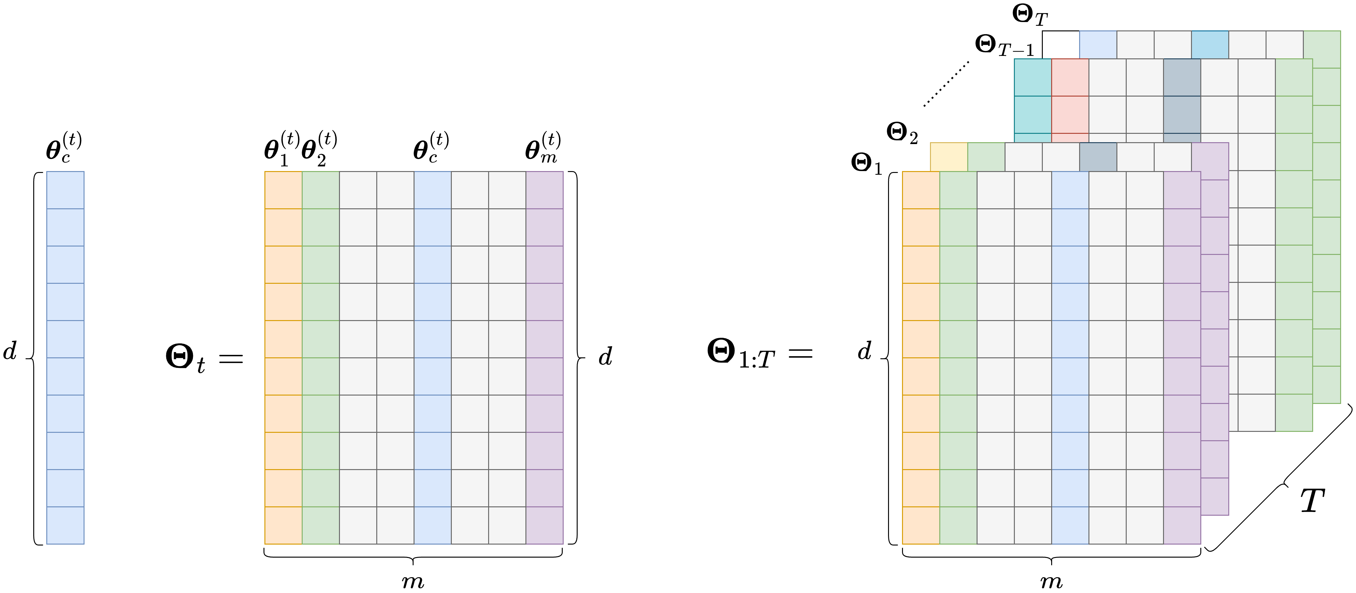
Figure 1: The $d$-dimensional vector of parameters $\bm{\theta}_{c}^{(t)}$ sent by client $c$ at round $t$ (left). The $d\times m$ matrix $\bm{\Theta}_{t}$ of all the $m$ client updates sent at round $t$ (middle). The $d\times m\times T$ tensor $\bm{\Theta}_{1:T}$ of all the client updates after $T$ rounds (right).

4.2 Byzantine Attack Model

Attacker’s goal. Like many studies on poisoning attacks (Rubinstein et al., 2009; Biggio et al., 2012, 2013; Xiao et al., 2015; Li et al., 2016; Yang et al., 2017; Jagielski et al., 2018; Fang et al., 2020), we consider the attacker’s goal is to manipulate the jointly learned global model with a high error rate indiscriminately for test examples. Such attacks are known as untargeted, as opposed to targeted poisoning attacks, where instead, the goal is to induce prediction errors only for some specific test instances.

Attacker’s capability. To achieve the goal above, we assume the attacker controls a fraction $b=\lceil r*K\rceil,r\in[0,1]$ of Byzantine clients, i.e., $0\leq b\leq K$. Like Sybil attacks (Douceur, 2002) to distributed systems, the attacker could inject $b$ fake clients into the FL system or compromise $b$ benign clients. The attacker can arbitrarily manipulate the local models sent by these malicious clients to the central server. More formally, let $x\in\mathcal{C}$ be one of the $b$ corrupted clients. On the generic $t$-th FL round, $x$ will send to $S$ its malicious local model update $\widetilde{\bm{\theta}}_{x}^{(t)}$ rather than the legitimate $\bm{\theta}_{x}^{(t)}$. As per how $x$ computes $\widetilde{\bm{\theta}}_{x}^{(t)}$, this can be done at least in two ways: via data or model poisoning, i.e., before or after local training. In the former case, $x$ finds $\widetilde{\bm{\theta}}_{x}^{(t)}$ as the result of performing its local training on a perturbed version $\widetilde{\mathcal{D}}_{x}$ of its private data $\mathcal{D}_{x}$ (e.g., via label flipping (Xiao et al., 2015)), i.e., $\widetilde{\bm{\theta}}_{x}^{(t)}=\text{argmin}_{\bm{\theta}^{(t)}}\mathcal{L}_{x}(\bm{\theta}^{(t)};\widetilde{\mathcal{D}}_{x})$. In the latter case, $x$ first legitimately computes $\bm{\theta}_{x}^{(t)}$ using Eq. (3) without modifying its local data $\mathcal{D}_{x}$; then it obtains $\widetilde{\bm{\theta}}_{x}^{(t)}$ by applying a post hoc perturbation $\bm{\varepsilon}\in\mathbb{R}^{d}$ to the correct local model update. For example, $\widetilde{\bm{\theta}}_{x}^{(t)}=\bm{\theta}_{x}^{(t)}+\bm{\varepsilon}$, where $\bm{\varepsilon}\sim\mathcal{N}(\bm{\mu},\bm{\Sigma})$ is a random Gaussian noise vector.
Notice that any data poisoning attack can be seen as a special case of a local model poisoning attack. However, recent studies (Bhagoji et al., 2019; Fang et al., 2020) show that direct local model poisoning attacks are more effective than indirect data poisoning attacks against FL. Therefore, we focus on the former in this work.

Attacker’s knowledge. We suppose the attacker knows the code, local training datasets, and local models on its controlled clients. Moreover, since this work is concerned with the robustness of the aggregation function, we consider the worst-case scenario (from an honest FL system’s perspective), where the attacker also knows the aggregation function used by the central server. Based on this knowledge, the attacker may design more effective (i.e., disruptive) poisoning strategies (Fang et al., 2020). Besides, this assumption is realistic as the FL service provider may want to publicly disclose the aggregation rule used to promote transparency and trust in the FL system (McMahan et al., 2017).

Attacker’s behavior. We suppose there is no anomaly in the client updates observed in the first $L<T$ rounds, i.e., either no malicious clients have joined the FL network yet ($b=r=0$) or, even if they have, they have been acting legitimately (e.g., to achieve stealthiness and elude possible detection mechanisms). Then, assuming the Byzantine attack starts after $L$ rounds, our goal is to detect anomalous model updates sent afterwards (i.e., at any round $L+j$, where $j>0$), and discard them from the input to the aggregation function (e.g., FedAvg).

4.3 Byzantine Model Updates as Matrix-Based Time Series Outliers

Our problem can be therefore formulated as a multidimensional time series anomaly detection task. At a high level, we want to equip the central server $S$ with an anomaly scoring function that, based on the historical observations of model updates seen so far from all the clients, estimates the degree of each client being malicious, i.e., its anomaly score. Such a score can in turn be used to restrict the set of candidate clients that are trustworthy for the aggregation.
More formally, at the generic $t$-th FL round, the central server $S$ must compute the anomaly score $s_{c}^{(t)}\in\mathbb{R}$ of every selected client $c\in\mathcal{C}^{(t)}$. To achieve that, we assume $S$ can leverage the past $w$ observations of model updates received, i.e., $\bm{\Theta}_{t-w:t-1}$, where $1\leq w\leq t-1$. The server will thus rank all the $m$ selected clients according to their anomaly scores (e.g., from the lowest to the highest). Hence, several strategies can be adopted to choose which model updates should be aggregated in preparation for the next round, i.e., to restrict from the initial set $\mathcal{C}^{(t)}$ to another (possibly smaller) set $\mathcal{C}_{*}^{(t)}\subseteq\mathcal{C}^{(t)}$ of trusted clients. For example, $S$ may consider only the model updates received from the top-$k$ clients ($1\leq k\leq m$) with the smallest anomaly score, i.e., $\mathcal{C}_{*}^{(t)}=\{c\in\mathcal{C}^{(t)}~{}|~{}s_{c}^{(t)}\leq s_{k}^{(t)}\}$, where $s_{k}^{(t)}$ indicates the $k$-th smallest anomaly score at round $t$. Alternatively, the raw anomaly scores computed by the server can be converted into well-calibrated probability estimates. Here, the server sets a threshold $\rho\in[0,1]$ and aggregates the weights only of those clients whose anomaly score is below $\rho$, i.e., $\mathcal{C}_{*}^{(t)}=\{c\in\mathcal{C}^{(t)}~{}|~{}s_{c}^{(t)}\leq\rho\}$. In the former case, the number of considered clients ($k$) is bound apriori, whereas the latter does not put any constraint on the size of final candidates $|\mathcal{C}_{*}^{(t)}|$. Eventually, $S$ will compute the updated global model $\bm{\theta}^{(t+1)}=\phi(\{\bm{\theta}_{c}^{(t)}~{}|~{}c\in\mathcal{C}_{*}^{(t)}\})$, where $\phi$ is any well-known aggregation function, e.g., FedAvg.
Several techniques can be used to compute the anomaly scoring function. In this work, we leverage the matrix autoregressive (MAR) framework for multidimensional time series forecasting proposed by Chen et al. (2021).

5 Proposed Method: FLANDERS

5.1 Matrix Autoregressive Model (MAR)

Many time series data involve observations that appear in a matrix form. For example, a set of atmospheric measurements like temperature, pressure, humidity, etc. (rows) are regularly reported by different weather stations spread across a given region (columns) every hour (time). In cases like this, the usual approach is to flatten matrix observations into long vectors, then use standard vector autoregressive models (VAR) for time series analysis. However, VAR has two main drawbacks: (i) it looses the original matrix structure as it mixes rows and columns, which instead may capture different relationships; (ii) it significantly increases the model complexity to a large number of parameters.
To overcome the two issues above, Chen et al. (2021) introduce the matrix autoregressive model (MAR). In its most generic form, MAR($p$) is a $p$-order autoregressive model:

$${\bm{X}}_{t}={\bm{A}}_{1}{\bm{X}}_{t-1}{\bm{B}}_{1}+\cdots+{\bm{A}}_{p}{\bm{X}}_{t-p}{\bm{B}}_{p}+{\bm{E}}_{t},$$

where ${\bm{X}}_{t}$ is a $d\times m$ matrix of observations at time $t$, ${\bm{A}}_{i}$ and ${\bm{B}}_{i}$ ($i\in\{1,\ldots,p\})$ are $d\times d$ and $m\times m$ autoregressive coefficient matrices, and ${\bm{E}}_{t}$ is a $d\times m$ white noise matrix. In this work, we consider the simplest MAR($1$) forecasting model, i.e., ${\bm{X}}_{t}={\bm{A}}{\bm{X}}_{t-1}{\bm{B}}+{\bm{E}}_{t}$, where the matrix of observations at time $t$ depends only on the previously observed matrix at time step $t-1$.
Let $\hat{\bm{X}}_{t}=\hat{{\bm{A}}}{\bm{X}}_{t-1}\hat{{\bm{B}}}$ be the estimated matrix of observations at time $t$, according to MAR for some coefficient matrices $\hat{{\bm{A}}}$ and $\hat{{\bm{B}}}$. Also, suppose we have access to $w>0$ historical matrix observations. Thus, we compute the best coefficients ${\bm{A}}$ and ${\bm{B}}$ by solving the following objective:

$${\bm{A}},{\bm{B}}=\operatorname*{arg\,min}_{\hat{{\bm{A}}},\hat{{\bm{B}}}}\Big{\{}\sum_{j=0}^{w-1}||{\bm{X}}_{t-j}-\hat{{\bm{A}}}{\bm{X}}_{t-j-1}\hat{{\bm{B}}}||^{2}_{\text{F}}\Big{\}},$$

where $||\cdot||_{\text{F}}$ indicates the Frobenius norm of a matrix. The coefficients ${\bm{A}}$ and ${\bm{B}}$ can thus be estimated via alternating least squares (ALS) optimization (Koren et al., 2009). We provide further details on MAR in Appendix B.

5.2 MAR-based Anomaly Score

So far, we have described an existing method for multidimensional time series forecasting, i.e., MAR. But how could MAR be helpful for detecting, and therefore discarding, local model sent by malicious FL clients? Indeed, MAR can be used to compute the anomaly score and thus identify possible outliers, as indicated in Section 4.3.
First of all, notice that the $d\times m$ matrix of $d$-dimensional model updates $\bm{\Theta}_{t}$ received by the central server from the $m$ clients at time $t$ nicely fits with the hypothesis under which MAR is supposed to work. We can set an analogy between FL training and our example in Section 5.1. Specifically, the matrix of observations of atmospheric measurements collected from distributed weather stations at a given time step resembles the matrix of local model weights sent by edge clients to the server at a given FL round. Therefore:

$$\bm{\Theta}_{t}={\bm{A}}\bm{\Theta}_{t-1}{\bm{B}}+{\bm{E}}_{t},$$ (5)

To estimate ${\bm{A}}$ and ${\bm{B}}$ we consider two separate cases: before malicious clients start sending corrupted updates (i.e., until the $L$-th time step), and from the $(L+1)$-th time step onward. We start focusing on the first $L$ matrices of observed weights, i.e., $\bm{\Theta}_{1},\bm{\Theta}_{2},\ldots,\bm{\Theta}_{L}$, and we set a fixed window size of observations $w$, which we will use for training. Then, following (5.1), we compute ${\bm{A}}$ and ${\bm{B}}$ as follows:

$${\bm{A}},{\bm{B}}=\operatorname*{arg\,min}_{\hat{{\bm{A}}},\hat{{\bm{B}}}}\Big{\{}\sum_{j=0}^{w-1}||{\bm{\Theta}}_{L-j}-\hat{{\bm{\Theta}}}_{L-j}||^{2}_{\text{F}}\Big{\}},$$ (6)

where $\hat{{\bm{\Theta}}}_{L-j}=\hat{{\bm{A}}}\bm{\Theta}_{L-1-j}\hat{{\bm{B}}}$ is the predicted weight matrix. Notice that $1\leq w\leq(L-1)$. In particular, if $w=1$ then ${\bm{A}}$ and ${\bm{B}}$ are computed using only $\bm{\Theta}_{L-1}$ and $\bm{\Theta}_{L}$. On the other side of the spectrum, if $w=L-1$ then ${\bm{A}}$ and ${\bm{B}}$ are estimated using all the $L$ previous observations: $\bm{\Theta}_{1},\bm{\Theta}_{2},\ldots,\bm{\Theta}_{L}$. This last setting is a natural choice for building a consistent MAR forecasting model under no attack. However, in the real world, the FL server does not know in advance if and when malicious clients kick in, i.e., the number $L$ of legitimate FL rounds is generally unknown apriori. Still, one could imagine that the initial parameters of a “clean” MAR model can be estimated during a bootstrapping stage in a “controlled” FL environment, where only well-known trusted clients are allowed to participate. Anyway, no matter how the MAR forecasting model is initially trained on clean observations, we use it to compute the anomaly score as follows. Consider the matrix of observed weights $\bm{\Theta}_{t}$ at the generic FL round $t>L$. We know that this matrix may contain one or more corrupted local model updates sent by malicious clients. Then, we compute the $m$-dimensional anomaly score vector ${\bm{s}}^{(t)}$ as follows:

$${\bm{s}}^{(t)}[c]=s_{c}^{(t)}=\delta(\bm{\Theta}_{t}[:,c],\hat{\bm{\Theta}}_{t}[:,c]),$$ (7)

where: $c$ is one of the $m$ clients; $\bm{\Theta}_{t}[:,c]$ indicates the $c$-th column of the observed $\bm{\Theta}_{t}$ and contains the $d$-dimensional vector of weights sent by client $c$; $\hat{\bm{\Theta}}_{t}={\bm{A}}\bm{\Theta}_{t-1}{\bm{B}}$ is the matrix predicted by MAR at time $t$, using the previous observation $\bm{\Theta}_{t-1}$ and the coefficients ${\bm{A}}$ and ${\bm{B}}$ learned so far; and $\delta(\cdot)$ is a function measuring the distance between the observed vector of weights sent to the server and the predicted vector of weights output by MAR. In this work, we set $\delta=||\bm{\Theta}_{t}[:,c]-\hat{\bm{\Theta}}_{t}[:,c]||_{2}^{2}$, where $||\cdot||_{2}^{2}$ is the squared $L^{2}$-norm. Other functions can be used (e.g., cosine distance), especially in high dimensional spaces, where $L^{p}$-norm with $p\in(0,1)$ has proven effective (Aggarwal et al., 2001). However, choosing the best $\delta$ is outside the scope of this work, and we leave it to future study.

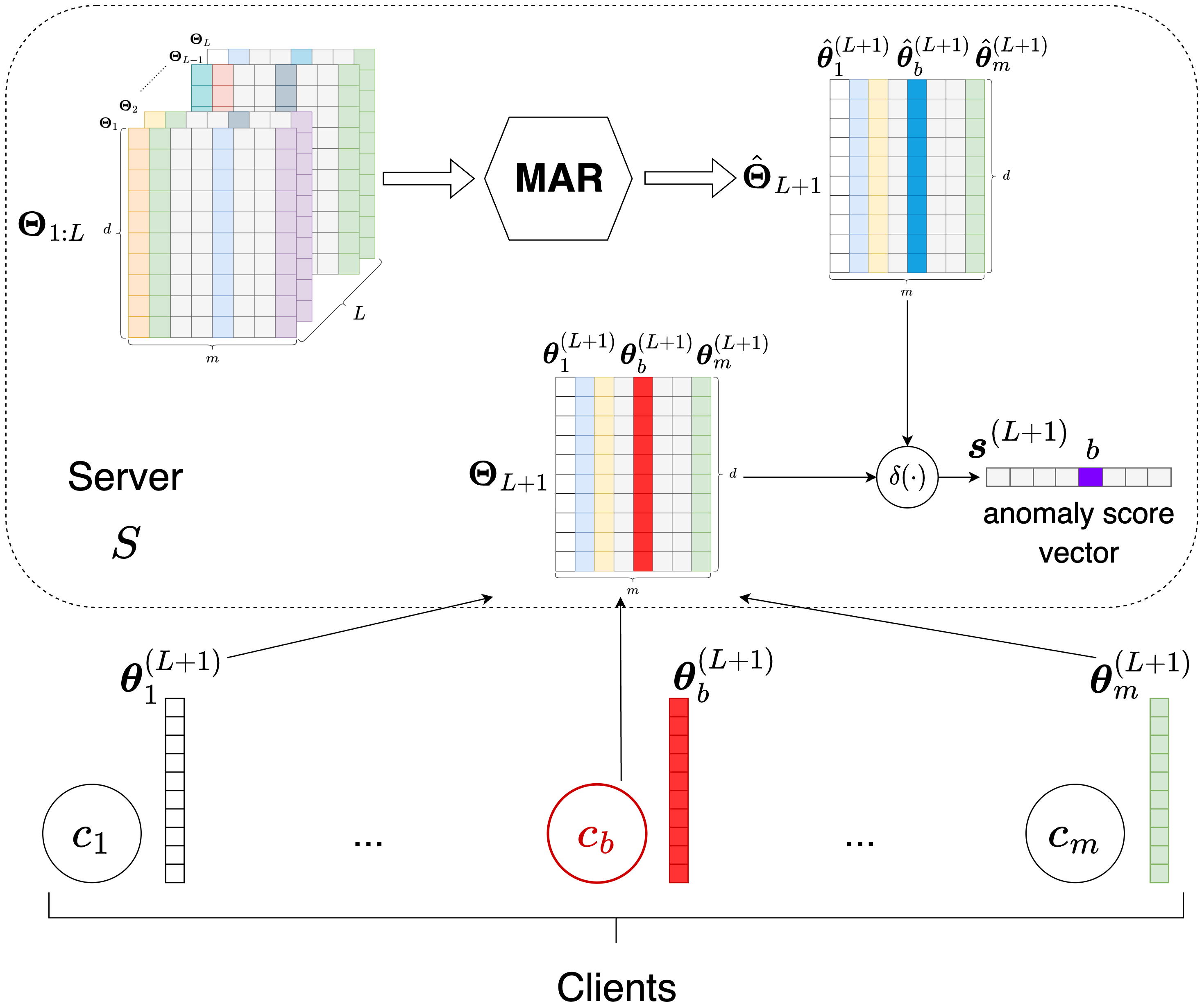
Figure 2: Overview of FLANDERS.

According to one of the filtering strategies discussed in Section 4.3, we retain only the $k$ clients with the smallest anomaly scores. The remaining $m-k$ clients will be discarded and not contribute to the aggregation performed by the server (e.g., FedAvg).
At the next round $t+1$, to compute the updated anomaly score vector as in Eq. (7), we need to refresh our MAR model, i.e., to update the coefficient matrices ${\bm{A}}$ and ${\bm{B}}$, based on the latest observed $\bm{\Theta}_{t}$, along with the other $w-1$ previous matrices of local updates. Since the initially observed matrix $\bm{\Theta}_{t}$ contains $m-k$ potentially malicious clients, we cannot use it as-is to update our MAR model. Otherwise, we may alter the estimated coefficients ${\bm{A}}$ and ${\bm{B}}$ by considering possibly corrupted matrix columns. The solution we propose to overcome this problem is to replace the original $\bm{\Theta}_{t}$ with $\bm{\Theta}^{\prime}_{t}$ before feeding it to train the new MAR model. Specifically, $\bm{\Theta}^{\prime}_{t}$ is obtained from $\bm{\Theta}_{t}$ by substituting the $m-k$ anomalous columns with the parameter vectors from the same clients observed at time $t-1$, which are supposed to be still legitimate. The advantage of this solution is twofold. On the one hand, a client labeled as malicious at FL round $t$ would likely still be considered so at $t+1$ if it keeps perturbing its local weights, thus improving robustness. On the other hand, our solution allows malicious clients to alternate legitimate behaviors without being banned, hence speeding up model convergence. Notice that the two considerations above might not be valid if we updated our MAR model using the original, partially corrupted $\bm{\Theta}_{t}$. Indeed, in the first case, the distance between two successive corrupted vectors of weights by the same client would realistically be small. So the client’s anomaly score will likely drop to non-alarming values, thereby increasing the number of false negatives. In the second case, the distance between a corrupted vector of weights and a legitimate one would likely be considerable. Therefore, a malicious client will maintain its anomaly score high even if it decides to act normally, thus impacting the number of false positives.
The overview of FLANDERS is depicted in Fig. 2.

6 Experiments

6.1 Experimental Setup

Datasets, Tasks, and FL Models. We consider a mix of four tabular and non-tabular (i.e., image) public datasets used for classification (Income, MNIST, and CIFAR-10) and regression (California Housing) tasks. Except for the MNIST and CIFAR-10 datasets that already come split into a training and a test portion, the remaining datasets are randomly shuffled and partitioned into two disjoint sets: 80% reserved for training and 20% for testing.
Eventually, for each dataset/task combination, we choose a dedicated FL model amongst the following: Logistic Regression (LogReg), Multilayer Perceptron (MLP), Convolutional Neural Network (CNN), and Linear Regression (LinReg). All models are trained by minimizing cross-entropy loss (in the case of classification tasks) or elastic net regularized mean squared error (in the case of regression). At each FL round, every client performs one iteration of cyclic coordinate descent (LogReg and LinReg) or one epoch of stochastic gradient descent (MLP and CNN).
The full details are shown in Table 1 of Appendix C.

FL simulation environment. To simulate a realistic FL environment, we integrate FLANDERS into Flower. Other valid FL frameworks are available (e.g., TensorFlow Federated and PySyft), but Flower was the most appropriate choice for our scope. Flower allows us to specify the number $K$ of FL clients, which in this work we set to $100$. Moreover, we assume that the server selects all these clients in every FL round; in other words, $K=m$. For the first $L=30$ rounds, no attack occurs; then, we monitor the performance of the global model for additional $20$ rounds, i.e., until $T=50$, while malicious clients possibly enter the FL system.
A complete description of our FL simulation environment is provided in Appendix D.

We run our experiments on a 4-node cluster; each node has a 48-core 64-bit AMD CPU running at 3.6 GHz with 512 GB RAM and an NVIDIA A100 GPU with 40 GB VRAM.

6.2 Attacks

We assess the robustness of FLANDERS under the following well-known attacks. Moreover, for each type of attack, we vary the number $b=\lceil r*m\rceil,r\in[0,1]$ of Byzantine clients by experimenting with several values of $r=\{0.05,0.1,0.2,0.3,0.4,0.5,0.6,0.7,0.8,0.9,0.95\}$.

Gaussian Noise Attack. This attack randomly crafts the local models on the compromised clients. Specifically, the attacker samples a random value from a Gaussian distribution $\varepsilon\sim\mathcal{N}(0,\sigma^{2})$ and sums it to the all the $d$ learned parameters. We refer to this attack as GAUSS.

“A Little Is Enough” Attack (Baruch et al., 2019). This attack lets the defender remove the non-Byzantine clients and shift the aggregation gradient by carefully crafting malicious values that deviate from the correct ones as far as possible. We call this attack LIE.

Optimization-based Attack (Fang et al., 2020). The authors formulate this attack as an optimization task, aiming to maximize the distance between the poisoned aggregated gradient and the aggregated gradient under no attack. By leveraging halving search, they obtain a crafted malicious gradient. We refer to this attack as OPT.

AGR Attack Series (Shejwalkar & Houmansadr, 2021). This improves the optimization program above by introducing perturbation vectors and scaling factors. Then, three instances are proposed: AGR-tailored, AGR-agnostic Min-Max, and Min-Sum, which maximize the deviation between benign and malicious gradients. In this work, we experiment with AGR Min-Max, which we call AGR-MM.

We detail the parameters of the attacks above in Appendix E.

6.3 Evaluation

We compare the robustness of FLANDERS against plain “vanilla” FedAvg and all the baselines already described in Section 3: Trimmed Mean, FedMedian, Krum, Bulyan, FLTrust, and MSCRED. For a fair comparison, we set the number of trusted clients to keep at each round to $k=1$. We discuss all the other critical parameters of these defense strategies in Appendix F.
For each classification task, we measure the best global model’s accuracy obtained with all the FL aggregation strategies after the $L$-th round (i.e., after the attack). We operate similarly for the regression task associated with the California Housing dataset, measuring the global model’s one minus mean absolute percentage error (1-MAPE).

Robustness. We show the result of our comparison in Fig. 3. Each row on this figure represents a dataset/task, whereas each column corresponds to a specific attack. Moreover, each plot depicts how the maximum accuracy (1-MAPE for the regression task) of the global model changes as the power of the attack (i.e., the percentage of Byzantine clients in the FL system) increases.

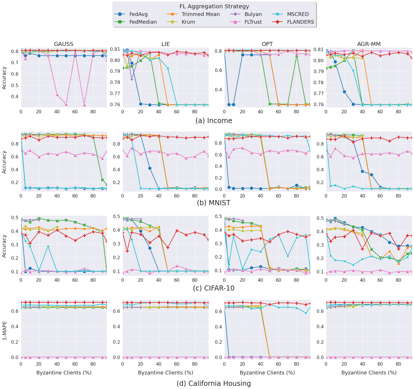
Figure 3: Comparing the robustness of FLANDERS against all the baselines on four datasets/tasks (rows) under four attacks (columns).

To comment on this result, we can distinguish between two cases: when the attack strength is low/moderate or when this is severe. In the former case, i.e., from $10\%$ up to $40\%$ of malicious clients, FLANDERS behaves similarly to its best-performing competitors. In fact, except for CIFAR-10, where FLANDERS performs slightly worse than other robust baselines, for all the other datasets/tasks, FLANDERS is either on par with (see Income and MNIST) or even constantly better (see California Housing) than baseline approaches. Instead, when the ratio of Byzantine clients gets above $40\%$, FLANDERS outperforms all the competitors. More generally, the robustness of FLANDERS is way more steady than that of other methods across the whole spectrum of the attack power. In addition, it is worth remarking that some approaches, like Krum and Bulyan, are not even designed to work under such severe attack scenarios (i.e., with more than $50\%$ and $25\%$ malicious clients, respectively). We further discuss the stability of the performance exhibited by FLANDERS in Appendix G.1.

Robustness vs. Cost. Evaluating the robustness is undoubtedly pivotal. However, any robust FL aggregation strategy may sacrifice the global model’s performance when no attack occurs. In other words, there is a price to pay in exchange for the level of security guaranteed. Thus, we introduce another evaluation metric that captures the robustness vs. cost trade-off. Our experiments show that FLANDERS achieves the best balance between robustness and cost under every attack when the ratio of corrupted clients is extremely severe (i.e., $80\%$). Due to space limitations, we report the full results of this analysis in Appendix G.2.

6.4 FLANDERS with Non-IID Local Training Data

A peculiarity of FL is that the local training datasets on different clients may not be independent and identically distributed (non-i.i.d.) (McMahan et al., 2017)). Hence, we also validate FLANDERS in this setting. Specifically, we simulate non-i.i.d. local training data of the CIFAR-10 dataset using the built-in capabilities provided by Flower. Indeed, Flower includes a dataset partitioning method based on Dirichlet sampling to simulate non-i.i.d. label distribution across federated clients as proposed by (Hsu et al., 2019). This technique uses a hyperparameter $\alpha_{D}$ to control client label identicalness. In this work, we set $\alpha_{D}=0.5$ to simulate a strong class label imbalance amongst clients.
We analyze the impact of non-i.i.d. training data on FLANDERS by measuring how the global model’s accuracy changes with the number of FL rounds, both under attack and with no malicious clients. In the first case, we consider all the attacks described in Section 6.2 with $20\%$ of Byzantine clients, and we vary the number of clients deemed to be legitimate at each round as $k\in\{1,5,20\}$. Due to space limitations, results are presented in Appendix G.3.

7 Conclusion and Future Work

We have introduced FLANDERS, a novel federated learning (FL) aggregation scheme robust to Byzantine attacks. FLANDERS treats the local model updates sent by clients at each FL round as a matrix-valued time series. Then, it identifies malicious clients as outliers of this time series by computing an anomaly score that compares actual observations with those estimated by a matrix autoregressive forecasting model. Experiments run on several datasets under different FL settings have demonstrated that FLANDERS matches the robustness of the most powerful baselines against Byzantine clients. Furthermore, FLANDERS remains highly effective even under extremely severe attacks (i.e., beyond $50\%$ malicious clients), as opposed to existing defense strategies that either fail or are not even designed to handle such settings as Krum and Bulyan.
In the future, we will address some limitations of this work. First, we expect to reduce the computational cost of FLANDERS further, especially for complex models with millions of parameters, leveraging the implementation tricks discussed in Appendix F. Then, we plan to extend FLANDERS using more expressive MAR($p$) models ($p>1$) and conduct a deeper analysis of its key parameters (e.g., $w$, $k$, and $\delta$).

Appendix A The Impact of Byzantine Clients at each FL Round

Under our assumptions, the FL system contains a total of $K$ clients, where $b$ of those are Byzantine controlled by an attacker ($0\leq b\leq K$). In addition, at each FL round, $m$ clients ($1\leq m\leq K$) are selected, and thus, some of the $m$ model updates received by the central server may be corrupted. The probability of this event can actually be computed by noticing that the outcome of the client selection at each round can be represented by a random variable $X\sim\text{Hypergeometric}(K,b,m)$, whose probability mass function is:

$$p_{X}(x)=\Pr(X=x)=\frac{\binom{b}{x}\binom{K-b}{m-x}}{\binom{K}{m}}.$$

The chance that, at a single round, at least one of the $b$ malicious clients ends up in the list of $m$ clients equals:

$$\Pr(X\geq 1)=1-\Pr(X=0)=1-\frac{\binom{b}{0}\binom{K-b}{m-0}}{\binom{K}{m}}=1-\frac{\binom{K-b}{m}}{\binom{K}{m}}.$$

For example, if the total number of clients is $K=100$, $b=5$ of them are malicious, and $m=20$ must be drawn at each round then $\Pr(X\geq 1)\approx 68\%$. In other words, there are about two out of three chances that at least one malicious client is picked at every FL round.

Appendix B Matrix Autoregressive Model (MAR)

In this work, we consider the simplest MAR($1$) forecasting model, which exhibits a bilinear structure as follows:

$${\bm{X}}_{t}={\bm{A}}{\bm{X}}_{t-1}{\bm{B}}+{\bm{E}}_{t}.$$

Thus, the key question here is how to estimate the best coefficient matrices ${\bm{A}}$ and ${\bm{B}}$. To achieve this goal, we first let $\hat{\bm{X}}_{t}=\hat{{\bm{A}}}{\bm{X}}_{t-1}\hat{{\bm{B}}}$ be the estimated matrix of observations at time $t$, according to MAR for some coefficient matrices $\hat{{\bm{A}}}$ and $\hat{{\bm{B}}}$. Hence, we can define an instance-level loss function as follows:

$$\ell(\hat{{\bm{A}}},\hat{{\bm{B}}};{\bm{X}}_{t})=||{\bm{X}}_{t}-\hat{{\bm{X}}}_{t}||^{2}_{\text{F}}=||{\bm{X}}_{t}-\hat{{\bm{A}}}{\bm{X}}_{t-1}\hat{{\bm{B}}}||^{2}_{\text{F}},$$ (8)

where $||\cdot||_{\text{F}}$ indicates the Frobenius norm of a matrix. More generally, if we have access to $w>0$ historical matrix observations, we can compute the overall loss function below:

$$\mathcal{L}(\hat{{\bm{A}}},\hat{{\bm{B}}};{\bm{X}}_{t},w)=\sum_{j=0}^{w-1}\ell(\hat{{\bm{A}}},\hat{{\bm{B}}};{\bm{X}}_{t-j}).$$ (9)

As we assume ${\bm{E}}_{t}$ is a white noise matrix, its entries are i.i.d. normal with zero-mean and constant variance. Eventually, ${\bm{A}}$ and ${\bm{B}}$ can be found as the solutions of the following objective:

$${\bm{A}},{\bm{B}}=\operatorname*{arg\,min}_{\hat{{\bm{A}}},\hat{{\bm{B}}}}\Big{\{}\mathcal{L}(\hat{{\bm{A}}},\hat{{\bm{B}}};{\bm{X}}_{t},w)\Big{\}}=\operatorname*{arg\,min}_{\hat{{\bm{A}}},\hat{{\bm{B}}}}\Big{\{}\sum_{j=0}^{w-1}||{\bm{X}}_{t-j}-\hat{{\bm{A}}}{\bm{X}}_{t-j-1}\hat{{\bm{B}}}||^{2}_{\text{F}}\Big{\}}.$$

To solve the optimization task defined in Eq. (B) above, with a slight abuse of notation, we may observe the following. A closed-form solution to find ${\bm{A}}$ can be computed by taking the partial derivative of the loss w.r.t. ${\bm{A}}$, setting it to $0$, and solving it for ${\bm{A}}$. In other words, we search for ${\bm{A}}$ such that:

$$\frac{\partial{\mathcal{L}({\bm{A}},{\bm{B}};{\bm{X}}_{t},w)}}{\partial{{\bm{A}}}}=0.$$

Using Eq. (9) and Eq. (8), the left-hand side of Eq. (B) can be rewritten as follows:

$$\frac{\partial{\mathcal{L}({\bm{A}},{\bm{B}};{\bm{X}}_{t},w)}}{\partial{{\bm{A}}}} =\frac{\partial{\sum_{j=0}^{w-1}||{\bm{X}}_{t-j}-{\bm{A}}{\bm{X}}_{t-j-1}{\bm{B}}||^{2}_{\text{F}}}}{\partial{{\bm{A}}}}=$$

$$=-2\sum_{j=0}^{w-1}({\bm{X}}_{t-j}-{\bm{A}}{\bm{X}}_{t-j-1}{\bm{B}}^{T}){\bm{B}}{\bm{X}}^{T}_{t-1}=$$

$$=-2\Bigg{[}\Bigg{(}\sum_{j=0}^{w-1}{\bm{X}}_{t-j}{\bm{B}}{\bm{X}}^{T}_{t-j-1}\Bigg{)}-{\bm{A}}\Bigg{(}\sum_{j=0}^{w-1}{\bm{X}}_{t-j-1}{\bm{B}}^{T}{\bm{B}}{\bm{X}}^{T}_{t-j-1}\Bigg{)}\Bigg{]}.$$ (11)

If we set Eq. (11) to $0$ and solve it for ${\bm{A}}$, we find:

$$-2\Bigg{[}\Bigg{(}\sum_{j=0}^{w-1}{\bm{X}}_{t-j}{\bm{B}}{\bm{X}}^{T}_{t-j-1}\Bigg{)}-{\bm{A}}\Bigg{(}\sum_{j=0}^{w-1}{\bm{X}}_{t-j-1}{\bm{B}}^{T}{\bm{B}}{\bm{X}}^{T}_{t-j-1}\Bigg{)}\Bigg{]}=0\iff$$

$$\Bigg{(}\sum_{j=0}^{w-1}{\bm{X}}_{t-j}{\bm{B}}{\bm{X}}^{T}_{t-j-1}\Bigg{)}-{\bm{A}}\Bigg{(}\sum_{j=0}^{w-1}{\bm{X}}_{t-j-1}{\bm{B}}^{T}{\bm{B}}{\bm{X}}^{T}_{t-j-1}\Bigg{)}=0.$$

Hence:

$$\Bigg{(}\sum_{j=0}^{w-1}{\bm{X}}_{t-j}{\bm{B}}{\bm{X}}^{T}_{t-j-1}\Bigg{)}-{\bm{A}}\Bigg{(}\sum_{j=0}^{w-1}{\bm{X}}_{t-j-1}{\bm{B}}^{T}{\bm{B}}{\bm{X}}^{T}_{t-j-1}\Bigg{)} =0$$ (12)

$$\Bigg{(}\sum_{j=0}^{w-1}{\bm{X}}_{t-j}{\bm{B}}{\bm{X}}^{T}_{t-j-1}\Bigg{)}={\bm{A}}\Bigg{(}\sum_{j=0}^{w-1}{\bm{X}}_{t-j-1}{\bm{B}}^{T}{\bm{B}}{\bm{X}}^{T}_{t-j-1}\Bigg{)}$$ (13)

$${\bm{A}}=\Bigg{(}\sum_{j=0}^{w-1}{\bm{X}}_{t-j}{\bm{B}}{\bm{X}}^{T}_{t-j-1}\Bigg{)}\Bigg{(}\sum_{j=0}^{w-1}{\bm{X}}_{t-j-1}{\bm{B}}^{T}{\bm{B}}{\bm{X}}^{T}_{t-j-1}\Bigg{)}^{-1}.$$ (14)

Notice that Eq. (14) is obtained by multiplying both sides of Eq. (13) by $\Big{(}\sum_{j=0}^{w-1}{\bm{X}}_{t-j-1}{\bm{B}}^{T}{\bm{B}}{\bm{X}}^{T}_{t-j-1}\Big{)}^{-1}$.

If we apply the same reasoning, we can also find a closed-form solution to compute ${\bm{B}}$. That is, we take the partial derivative of the loss w.r.t. ${\bm{B}}$, set it to $0$, and solve it for ${\bm{B}}$:

$$\frac{\partial{\mathcal{L}({\bm{A}},{\bm{B}};{\bm{X}}_{t},w)}}{\partial{{\bm{B}}}}=0.$$

Eventually, we obtain the following:

$${\bm{B}}=\Bigg{(}\sum_{j=0}^{w-1}{\bm{X}}^{T}_{t-j}{\bm{A}}{\bm{X}}_{t-j-1}\Bigg{)}\Bigg{(}\sum_{j=0}^{w-1}{\bm{X}}^{T}_{t-j-1}{\bm{A}}^{T}{\bm{A}}{\bm{X}}_{t-j-1}\Bigg{)}^{-1}.$$

We now have two closed-form solutions; one for ${\bm{A}}$ (see Eq. (14)) and one for ${\bm{B}}$ (see Eq. (B)). However, the solution to ${\bm{A}}$ involves ${\bm{B}}$, and the solution to ${\bm{B}}$ involves ${\bm{A}}$. In other words, we must know ${\bm{B}}$ to compute ${\bm{A}}$ and vice versa.

We can use the standard Alternating Least Squares (ALS) algorithm (Koren et al., 2009) to solve such a problem. The fundamental idea of ALS is to iteratively update the least squares closed-form solution of each variable alternately, keeping fixed the other. At the generic $i$-th iteration, we compute:

$${\bm{A}}^{(i+1)}=\Bigg{(}\sum_{j=0}^{w-1}{\bm{X}}_{t-j}{\bm{B}}^{(i)}{\bm{X}}^{T}_{t-j-1}\Bigg{)}\Bigg{(}\sum_{j=0}^{w-1}{\bm{X}}_{t-j-1}({\bm{B}}^{(i)})^{T}{\bm{B}}^{(i)}{\bm{X}}^{T}_{t-j-1}\Bigg{)}^{-1};$$

$${\bm{B}}^{(i+1)}=\Bigg{(}\sum_{j=0}^{w-1}{\bm{X}}^{T}_{t-j}{\bm{A}}^{(i+1)}{\bm{X}}_{t-j-1}\Bigg{)}\Bigg{(}\sum_{j=0}^{w-1}{\bm{X}}^{T}_{t-j-1}({\bm{A}}^{(i+1)})^{T}{\bm{A}}^{(i+1)}{\bm{X}}_{t-j-1}\Bigg{)}^{-1};$$

ALS repeats the two steps above until some convergence criterion is met, e.g., after a specific number of iterations $N$ or when the distance between the values of the variables computed in two consecutive iterations is smaller than a given positive threshold, i.e., $d({\bm{A}}^{(i+1)}-{\bm{A}}^{(i)})<\varepsilon$ and $d({\bm{B}}^{(i+1)}-{\bm{B}}^{(i)})<\varepsilon$, where $d(\cdot)$ is any suitable matrix distance function and $\varepsilon\in\mathbb{R}_{>0}$.

Appendix C Datasets, Tasks, and FL Models

In Table 1, we report the full details of our experimental setup concerning the datasets used, their associated tasks, and the models (along with their hyperparameters) trained on the simulated FL environment. The description of the hyperparameters is shown in Table 2.

Table 1: Experimental setup: datasets, tasks, and FL models considered.

Dataset	N. of Instances (training/test)	N. of Features	Task	FL Model	Hyperparameters
Income (1996)	$39,074$/$9,768$	$14$ (numerical+categorical)	binary classification	LogReg	{$\lambda_{1}$=$1.0$; $\lambda_{2}$=$0.0$; opt=CCD}
MNIST (1998)	$60,000$/$10,000$	$28$x$28$ (numerical)	multiclass classification	MLP	{batch=$32$; layers=$3$; opt=Adam; dropout=$0.2$; $\eta$=$10^{-3}$}
CIFAR-10 (2009)	$50,000$/$10,000$	$32$x$32$x$3$ (numerical)	multiclass classification	CNN	{batch=$32$; layers=$6$; opt=SGD; $\eta$=$10^{-2}$}
California Housing (1997)	$15,740$/$3,935$	$18$ (numerical)	regression	LinReg	{$\lambda_{1}$=$0.5$; $\lambda_{2}$=$0.5$; opt=CCD}

Table 2: Description of hyperparameters.

Hyperparameter	Description
$\lambda_{1}$	$L^{1}$-regularization term (LASSO)
$\lambda_{2}$	$L^{2}$-regularization term (Ridge)
$\eta$	learning rate
opt	optimizer: cyclic coordinate descent (CCD); stochastic gradient descent (SGD); Adam
batch	batch size
layers	number of neural network layers
dropout	neural network node’s dropout probability

LogReg and LinReg are optimized via cyclic coordinate descent (CCD) by minimizing $L^{1}$-regularized binary cross-entropy loss and $L^{1}$/$L^{2}$-regularized mean squared error, respectively. MLP is a $3$-layer fully-connected feed-forward neural network trained by minimizing multiclass cross-entropy loss using Adam optimizer with batch size equal to $32$. CNN is a $6$-layer convolutional neural network trained by minimizing multiclass cross-entropy loss via stochastic gradient descent (SGD) with batch size equal to $32$.

For LogReg and LinReg, at each FL round, every client performs one iteration of CCD (i.e., each model parameter is updated independently from the others). Instead, for MLP and CNN, at each FL round, every client performs one training epoch of Adam/SGD, which corresponds to the number of iterations needed to “see” all the training instances once, when divided into batches of size $32$. In any case, the updated local model is sent to the central server for aggregation.

We run our experiments on a 4-node cluster; each node has a 48-core 64-bit AMD CPU running at 3.6 GHz with 512 GB RAM and an NVIDIA A100 GPU with 40 GB VRAM.

Appendix D FL Simulation Environment

Table 3: Main properties of our FL environment simulated on Flower.

Total N. of Clients	$K=100$
N. of Selected Clients (at each round)	$m=K=100$
Ratio of Byzantine Clients	$r=\{0.05,0.1,0.2,0.3,0.4,0.5,0.6,0.7,0.8,0.9,0.95\}$
Total N. of FL Rounds	$T=50$
N. of Legitimate FL Rounds (with no attacks)	$L=30$
Historical Window Size of Past FL Rounds	$w=L=30$
Dataset Distribution across Clients	i.i.d. for all datasets (in addition, non-i.i.d. only for CIFAR-10)

Each training portion of the datasets listed in Table 1 is distributed across the FL clients so that every client observes the same local data distribution. For example, in the case of MNIST, we let each client observe the same proportion of digit samples. However, this setting – known as i.i.d. – may be an unrealistic scenario in FL systems, and, most likely, local training datasets on different clients follow different distributions, i.e., they are non-i.i.d. Notice that there are many types of “non-i.i.d.-ness” that may involve: (i) labels, (ii) number of instances, and (iii) features. Concerning (i), this occurs when the distribution of labels is very unbalanced across clients (i.e., each client observes only a subset of the possible outputs). As for (ii), this happens when some clients have more data than others. Finally, (iii) represents a situation where similar feature patterns are grouped and shared amongst a few clients. In this work, we experiment with the first type of non-i.i.d.-ness limitedly to the CIFAR-10 dataset, which is already implemented in Flower (see Appendix G.3).

We report the main properties of our FL environment simulated on Flower in Table 3.

Appendix E Attack Settings

Below, we describe the critical parameters for each attack considered, which are also summarized in Table 4.

GAUSS. This attack has only one parameter: the magnitude $\sigma$ of the perturbation to apply. We set $\sigma=10$ for all the experiments.

LIE. This method has no parameters to set.

OPT. The parameter $\tau$ represents the minimum value that $\lambda$ can assume. Below this threshold, the halving search stops. As suggested by the authors, we set $\tau=10^{-5}$.

AGR-MM. In addition to the threshold $\tau$, AGR-MM uses the so-called perturbation vectors ($\nabla^{p}$) in combination with the scaling coefficient $\gamma$ to optimize. We set $\tau=10^{-5}$ and $\nabla^{p}=\{std\}$, which is the vector obtained by computing the parameters’ inverse of the standard deviation. For Krum, we set $\nabla^{p}=\{uv\}$, which is the inverse unit vector perturbation.

Table 4: Key parameter settings for each attack strategy considered.

Attack	Parameters
GAUSS	$\sigma=10$
LIE	N/A
OPT	$\tau=10^{-5}$
AGR-MM	$\tau=10^{-5};\nabla^{p}=\{uv,std\};\gamma=5$

Appendix F Defense Settings

Below, we describe the critical parameters for each baseline considered.

Trimmed Mean. The key parameter of this defense strategy is the number $k$, which is used to select the closest parameters to the median. In this work, we set $k=1$ to be homogeneous with other baselines.

FedMedian. This method has no parameters to set.

Krum. We set the number of Byzantine clients to $b=\lceil r^{\prime}*m\rceil$, where $r^{\prime}\subset r=\{0.05,0.1,0.2,0.3,0.4\}$, i.e., $b=\{5,10,20,30,40\}$.

Bulyan. The two crucial parameters of this hybrid robust aggregation rule are $\alpha$ and $\beta$. The former determines the number of times Krum is applied to generate $\alpha$ local models; the latter is used to determine the number of parameters to select closer to the median. In this work, we set $\alpha=m-2*b,\beta=\alpha-2*b$, where $b=\{5,10,20\}$.

FLTrust. A key parameter is the so-called root dataset. In this work, we assume the server samples the root dataset from the union of the clients’ clean local training data uniformly at random as in (Cao et al., 2020). We set the global learning rate to $\alpha=2\times 10^{-3}$ for MNIST and CIFAR-10 and $\alpha=1.0$ for Income and California Housing. Furthermore, the number of training epochs performed by the server is the same as that performed by the clients, i.e., $R_{l}=1$.

MSCRED. Since MSCRED is designed to work with vector-valued rather than matrix-valued time series, we need to adapt it to work in our setting. Specifically, we transform (i.e., flatten) our matrix observations into vectors and apply MSCRED by setting $w=1$. Note, however, that $w$ is the size of the window used to compute the signature matrices, meaning that the generic signature matrix is dependent on the previous one. In FLANDERS, instead, it indicates the number of previous steps to consider for estimating the coefficient matrices ${\bm{A}}$ and ${\bm{B}}$.

FLANDERS. We set the window size $w=30$ and the number of clients to keep at every round $k=1$ for a fair comparison with other baselines. Furthermore, we use a sampling value $\widetilde{d}\leq d$ that indicates how many parameters we store in the history, the number $N$ of ALS iterations, and $\alpha$ and $\beta$ which are regularization factors. Random sampling is used to select the subset of parameters considered; this step is necessary when the model to train is too big, otherwise leading to extremely large tensors that would exhaust the server memory. On the other hand, the regularization factors are needed when the model parameters, the number of clients selected, or $\widetilde{d}$ cause numerical problems in the ALS algorithm, whose number of iterations is set to $N=100$. We always set $\alpha=1$ and $\beta=1$, meaning that there is no regularization since, in our experience, it reduces the capability of predicting the right model. For this reason, we set $\widetilde{d}=500$ when we train CIFAR-10 and MNIST. Finally, we set the distance function $\delta$ used to measure the difference between the observed vector of weights sent to the server and the predicted vector of weights output by MAR to squared $L^{2}$-norm.

Table 5 summarizes the values of the key parameters discussed above and those characterizing our method FLANDERS.

Table 5: Key parameter settings for each defense strategy considered.

Defense	Parameters
FedAvg	N/A
Trimmed Mean	$\beta=k=1$
FedMedian	N/A
Krum	$b=\{5,10,20,30,40\}$
Bulyan	$b=\{5,10,20\};\alpha=m-2*b;\beta=\alpha-2*b$
FLTrust	$\alpha=\{1.0,2\times 10^{-3}\};R_{l}=1;$ root dataset randomly sampled from $\bigcup_{c=1}^{K}\mathcal{D}_{c}$
MSCRED	$w=1$
FLANDERS	$w=30$; $k=1$; $\widetilde{d}=\{0,500\}$; $N=100$; $\alpha=1$; $\beta=1$; $\delta=\text{squared }L^{2}$-norm

Appendix G Additional Experimental Results

G.1 Performance Stability

In this section, we further show how stable is the robustness of FLANDERS even under highly severe attack scenarios. Specifically, for each dataset/task, we plot the distribution of the global model’s accuracy obtained with all the FL aggregation rules considered in two attack settings: when the ratio of Byzantine clients is below $50\%$ (see Fig. 4) or equal to or above $50\%$ (see Fig. 5). We may notice that FLANDERS exhibits a low variance across the two settings, thus indicating high stability (i.e., more predictable behavior) compared to other baselines.

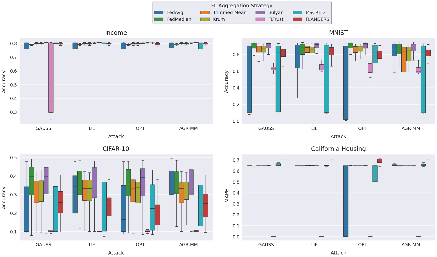
Figure 4: Distribution of the global model’s performance as measured with all the FL aggregation strategies under every attack when the ratio of Byzantine client is below $50\%$.

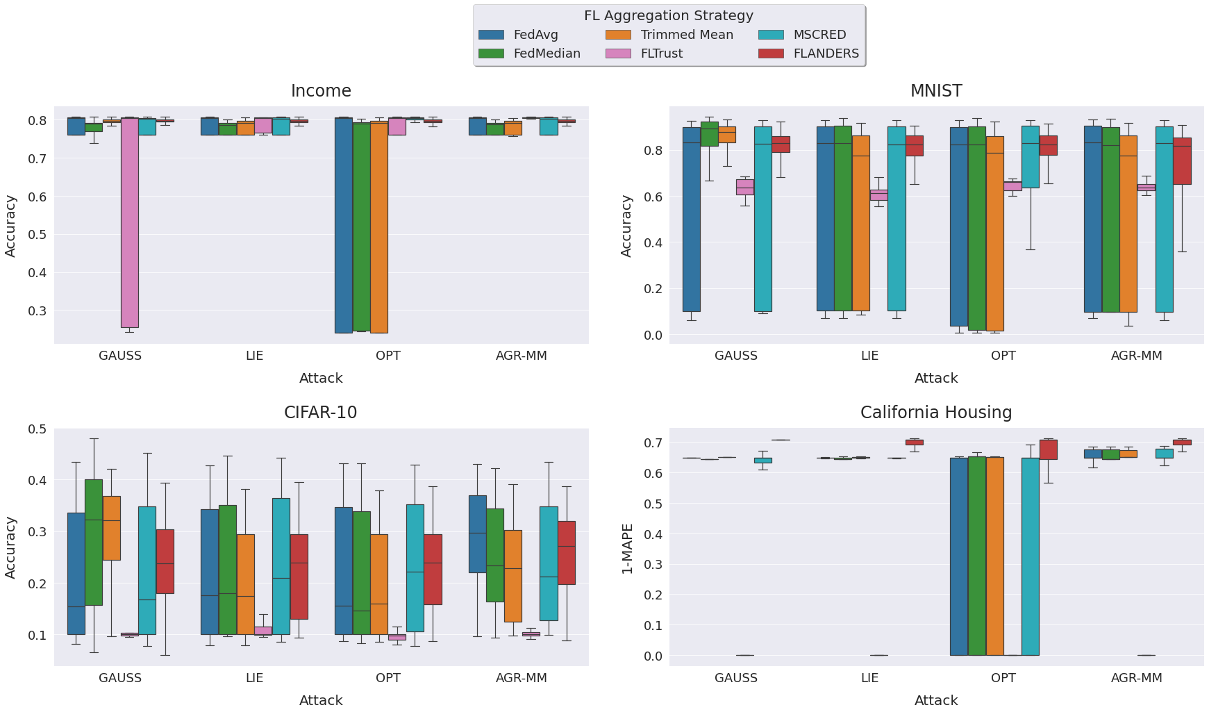
Figure 5: Distribution of the global model’s performance as measured with all the FL aggregation strategies under every attack when the ratio of Byzantine client is equal to or above $50\%$.

G.2 Robustness vs. Cost

Showing the global model’s performance drift before and after the attack helps understand the robustness of a specific FL aggregation scheme. However, this may not consider a possible cost due to the degradation introduced by the secure FL aggregation when no attack occurs. In other words, suppose that the best global model’s accuracy without attack is obtained with plain FedAvg, and let this value be $0.92$. Then, suppose that the accuracy drops to $0.65$ when Byzantine clients enter the FedAvg-based FL system. Undoubtedly, this is a remarkable accuracy loss. Now, consider some robust FL aggregation that achieves an accuracy of $0.71$ when no attack occurs and $0.66$ under attack. Clearly, this is far more robust than FedAvg as the accuracy values measured before and after the attack are closer than those obtained with FedAvg. In fact, we would draw a similar conclusion even if the accuracy under attack was $0.63$ instead of $0.66$ (i.e., if it was lower than the value observed with FedAvg). Still, we should also consider the accuracy drop observed with no attack (from $0.92$ to $0.71$).

Inspired by (Shejwalkar & Houmansadr, 2021), we design a unified metric that combines both the robustness and cost of an FL aggregation strategy. Specifically, let $v^{*}_{\text{pre}}$ be the overall best global model’s performance as measured within the $L$-th round (i.e., before any attack) for the generic task. Then, we compute $v^{\phi}_{\text{pre}}$ and $v^{\phi}_{\text{post}}$, namely the global model’s performance observed before and after a specific attack, using a fixed aggregation strategy $\phi$, where $\phi$ = {FedAvg, FedMedian, Trimmed Mean, Krum, Bulyan, FLTrust, MSCRED, FLANDERS}.

Thus, we define $R^{\phi}$ and $C^{\phi}$ respectively as the robustness and the cost of the aggregation strategy $\phi$, as follows:

$$R^{\phi}=\frac{v^{\phi}_{\text{post}}}{v^{\phi}_{\text{pre}}};~{}~{}~{}C^{\phi}=\frac{v^{*}_{\text{pre}}}{v^{\phi}_{\text{pre}}}-1.$$

The former captures the resiliency of an aggregation strategy to a given attack; the latter quantifies the drop w.r.t. the optimal model’s performance under no attack. Notice that $R^{\phi}=1$ iff the performance of the global model is unaffected by the attack, i.e., it is the same before and after the attack. Otherwise, $R^{\phi}<1$ indicates the defense mechanism struggles to compensate for the attack, and if $R^{\phi}>1$, the aggregation is so robust that the model keeps improving its performance even under attack. On the other hand, assuming $v^{*}_{\text{pre}}\geq v^{\phi}_{\text{pre}}$ for any $\phi$, $C^{\phi}\geq 0$ and $C^{\phi}=0$ iff the aggregation strategy achieves optimal performance under no attack. Eventually, we can calculate the net gain $G^{\phi}$ of an aggregation strategy as:

$$G^{\phi}=R^{\phi}-C^{\phi}.$$

Obviously, the larger $G^{\phi}$ the better.

It is worth remarking that, for each classification task, we measure the global model’s accuracy, whereas, for the regression task associated with the California Housing dataset, we compute the global model’s one minus mean absolute percentage error (1-MAPE). We report the result of this analysis in Table 6, focusing on two attack settings: when the ratio of Byzantine clients is $20\%$ and $80\%$, i.e., when $b=20$ and $b=80$.

Table 6: Evaluation of all the FL aggregation strategies on every dataset/task under four types of attack and two Byzantine settings: $20\%$ and $80\%$ malicious clients. The value in each cell is computed as the difference between the robustness and the cost of a specific defense mechanism as defined above, or N/A if that defense does not support the attack. Higher figures correspond to better performance.

Dataset	FL Aggregation	No Attack	GAUSS		LIE		OPT		AGR-MM
			$b=20$	$b=80$	$b=20$	$b=80$	$b=20$	$b=80$	$b=20$	$b=80$
Income	FedAvg	${\bf 1.00}$	$0.94$	$0.94$	$0.94$	$0.94$	$0.94$	$0.29$	$0.95$	$0.94$
	FedMedian	$0.98$	$0.98$	$0.99$	$0.99$	$0.94$	$0.98$	$0.93$	$0.99$	$0.94$
	Trimmed Mean	$0.99$	${\bf 1.00}$	$0.99$	${\bf 1.00}$	$0.94$	$0.99$	$0.29$	$0.99$	$0.94$
	Krum	$0.99$	$0.99$	N/A	$0.99$	N/A	$0.99$	N/A	$0.99$	N/A
	Bulyan	${\bf 1.00}$	${\bf 1.00}$	N/A	${\bf 1.00}$	N/A	$0.99$	N/A	${\bf 1.00}$	N/A
	FLTrust	${\bf 1.00}$	$0.99$	$0.96$	${\bf 1.00}$	$0.99$	$0.99$	$0.95$	${\bf 1.00}$	${\bf 1.00}$
	MSCRED	${\bf 1.00}$	$0.99$	$0.98$	${\bf 1.00}$	$0.94$	${\bf 1.00}$	${\bf 1.00}$	$0.99$	$0.94$
	FLANDERS	${\bf 1.00}$	${\bf 1.00}$	${\bf 1.00}$	$0.99$	${\bf 1.00}$	$0.99$	$0.99$	$0.99$	${\bf 1.00}$
MNIST	FedAvg	$1.01$	$0.11$	$0.10$	$1.00$	$0.12$	$0.00$	$0.07$	$0.97$	$0.10$
	FedMedian	${\bf 1.02}$	${\bf 1.01}$	$0.97$	${\bf 1.01}$	$0.10$	$1.01$	$0.02$	${\bf 1.01}$	$0.11$
	Trimmed Mean	$1.01$	$0.98$	${\bf 1.00}$	$1.00$	$0.09$	$0.99$	$-0.01$	$0.99$	$0.08$
	Krum	$1.00$	$0.99$	N/A	$1.00$	N/A	$0.99$	N/A	$0.97$	N/A
	Bulyan	$1.01$	${\bf 1.01}$	N/A	${\bf 1.01}$	N/A	${\bf 1.01}$	N/A	$1.00$	N/A
	FLTrust	$0.61$	$0.42$	$0.54$	$0.53$	$0.44$	$0.69$	$0.60$	$0.47$	$0.51$
	MSCRED	$1.00$	$0.11$	$0.10$	$0.11$	$0.10$	$1.00$	$0.97$	$0.10$	$0.10$
	FLANDERS	$0.96$	$0.91$	$0.96$	$0.99$	${\bf 0.96}$	$0.95$	${\bf 0.98}$	$0.99$	${\bf 0.97}$
CIFAR-10	FedAvg	${\bf 1.14}$	$0.20$	$0.20$	$0.94$	$0.21$	$0.24$	$0.21$	${\bf 1.10}$	${\bf 0.65}$
	FedMedian	$1.12$	${\bf 1.16}$	${\bf 0.96}$	${\bf 1.10}$	$0.16$	$1.08$	$0.21$	$1.08$	$0.37$
	Trimmed Mean	$1.00$	$1.02$	$0.95$	$0.98$	$0.10$	$0.99$	$0.09$	$0.97$	$0.17$
	Krum	$0.98$	$0.99$	N/A	$0.99$	N/A	$0.92$	N/A	$1.00$	N/A
	Bulyan	${\bf 1.14}$	$1.14$	N/A	$1.14$	N/A	${\bf 1.12}$	N/A	$1.07$	N/A
	FLTrust	$-2.16$	$-1.96$	$-2.42$	$-2.08$	$-2.40$	$-2.21$	$-2.40$	$-2.21$	$-2.42$
	MSCRED	$0.89$	$0.28$	$0.18$	$0.26$	$0.23$	$0.28$	$0.77$	$0.43$	$0.37$
	FLANDERS	$0.83$	$0.92$	$0.86$	$0.81$	${\bf 0.80}$	$0.58$	${\bf 0.79}$	$0.79$	$0.25$
California Housing	FedAvg	$0.90$	$0.90$	$0.90$	$0.91$	$0.91$	$-0.09$	$-0.09$	$0.96$	$0.96$
	FedMedian	$0.90$	$0.90$	$0.90$	$0.90$	$0.90$	$0.91$	$-0.07$	$0.93$	$0.96$
	Trimmed Mean	$0.91$	$0.91$	$0.91$	$0.90$	$0.91$	$0.93$	$-0.09$	$0.93$	$0.96$
	Krum	$0.91$	$0.91$	N/A	$0.90$	N/A	$0.91$	N/A	$0.91$	N/A
	Bulyan	$0.91$	$0.91$	N/A	$0.91$	N/A	$0.91$	N/A	$0.93$	N/A
	FLTrust	N/A	N/A	N/A	N/A	N/A	N/A	N/A	N/A	N/A
	MSCRED	$0.94$	$0.94$	$0.93$	$0.99$	${\bf 1.00}$	$0.94$	$0.90$	$0.96$	$0.96$
	FLANDERS	${\bf 1.00}$	${\bf 1.00}$	${\bf 1.00}$	${\bf 1.00}$	${\bf 1.00}$	${\bf 1.01}$	${\bf 0.99}$	${\bf 1.00}$	${\bf 1.00}$

G.3 FLANDERS with Non-IID Local Training Data

We simulate non-i.i.d. local training data distributions of the CIFAR-10 dataset using the built-in capabilities of Flower. Specifically, Flower includes a dataset partitioning method based on Dirichlet sampling to simulate non-i.i.d. label distribution across federated clients as proposed by (Hsu et al., 2019). Note that this is a common practice in FL research to obtain synthetic federated datasets (Wang et al., 2020; Reddi et al., 2021).

We assume every client training example is drawn independently with class labels following a categorical distribution over $N$ classes parameterized by a vector $\bm{q}$ such that $q_{i}\geq 0,i\in[1,\ldots,N]$ and $||\bm{q}||_{1}=1$.

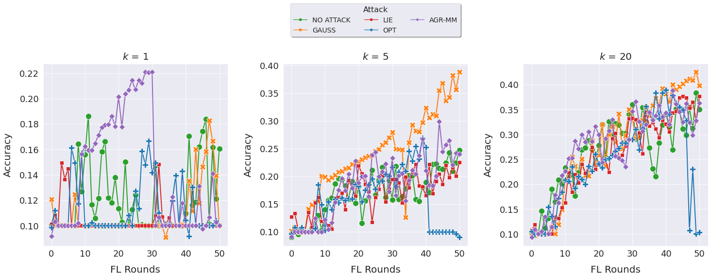
Figure 6: Global model’s accuracy on CIFAR-10 dataset with $20\%$ Byzantine clients and non-i.i.d. local training data using FLANDERS when $k=1$ (left), $k=5$ (middle), and $k=20$ (right).

To synthesize a population of non-identical clients, we draw $\bm{q}\sim\text{Dir}(\alpha_{D},\bm{p})$ from a Dirichlet distribution, where $\bm{p}$ characterizes a prior class distribution over $N$ classes, and $\alpha_{D}>0$ is a concentration parameter controlling the identicalness amongst clients. With $\alpha_{D}\rightarrow\infty$, all clients have identical label distributions; on the other extreme, with $\alpha_{D}\rightarrow 0$, each client holds examples from only one class chosen at random. In our experiment, we set $\alpha_{D}=0.5$ to simulate a strong class label imbalance amongst clients. Specifically, the CIFAR-10 dataset contains $60,000$ images ($50,000$ for training and $10,000$ for testing) from $N=10$ classes. We start from balanced populations consisting of $K=100$ clients, each holding $500$ images. Then, we set the prior distribution $\bm{p}$ to be uniform across $10$ classes. For every client, we sample $\bm{q}\sim\text{Dir}(0.5,\bm{p})$ and assign the client with the corresponding number of images from $10$ classes.

We analyze the impact of non-i.i.d. training data on FLANDERS by measuring how the global model’s accuracy changes with the number of FL rounds, both under attack and with no malicious clients. In the first case, we consider all the attacks described in Section 6.2 with $20\%$ of Byzantine clients (i.e., $b=20$), and we vary the number of clients deemed to be legitimate at each round as $k\in\{1,5,20\}$. The result of this study is shown in Fig. 6. We may observe that model training under a highly non-i.i.d. setting results in low and oscillating accuracy, disregarding the type of attack when the number of clients deemed to be legitimate is small (i.e., when $k=1$). The negative impact of non-i.i.d. is mitigated when we increase the number of legitimate clients $k$ included in the aggregation, except for the OPT attack, which preserves its detrimental effect on the global model’s accuracy. This result can be explained as follows. Intuitively, the more (legitimate) client updates we consider for aggregation, the better we cope with possible parameter variation due to local non-i.i.d. training.

References

- inc (1996) Adult Income Dataset. [Online]. Available from: https://archive.ics.uci.edu/ml/datasets/adult, 1996.
- cal (1997) California Housing Prices Dataset. [Online]. Available from: https://www.kaggle.com/datasets/camnugent/california-housing-prices, 1997.
- mni (1998) MNIST Dataset. [Online]. Available from: http://yann.lecun.com/exdb/mnist/, 1998.
- cif (2009) CIFAR-10 Dataset. [Online]. Available from: https://www.cs.toronto.edu/~kriz/cifar.html, 2009.
- Aggarwal et al. (2001) Aggarwal, C. C., Hinneburg, A., and Keim, D. A. On the Surprising Behavior of Distance Metrics in High Dimensional Space. In Proc. of ICDT’01, pp. 420–434. Springer, 2001.
- Baruch et al. (2019) Baruch, G., Baruch, M., and Goldberg, Y. A Little Is Enough: Circumventing Defenses For Distributed Learning. In NeurIPS’19, pp. 8632–8642, 2019. URL https://proceedings.neurips.cc/paper/2019/hash/ec1c59141046cd1866bbbcdfb6ae31d4-Abstract.html.
- Basu & Michailidis (2015) Basu, S. and Michailidis, G. Regularized Estimation in Sparse High-Dimensional Time Series Models. The Annals of Statistics, 43(4):1535–1567, 2015. URL https://doi.org/10.1214/15-AOS1315.
- Bhagoji et al. (2019) Bhagoji, A. N., Chakraborty, S., Mittal, P., and Calo, S. Analyzing Federated Learning through an Adversarial Lens. In ICML’19, pp. 634–643. PMLR Press, 2019.
- Biggio et al. (2012) Biggio, B., Nelson, B., and Laskov, P. Poisoning Attacks against Support Vector Machines. In ICML’12, pp. 1467–1474. Omnipress, 2012. URL http://icml.cc/2012/papers/880.pdf.
- Biggio et al. (2013) Biggio, B., Didaci, L., Fumera, G., and Roli, F. Poisoning Attacks to Compromise Face Templates. In ICB’13, pp. 1–7. IEEE, 2013. URL https://doi.org/10.1109/ICB.2013.6613006.
- Blanchard et al. (2017) Blanchard, P., El Mhamdi, E. M., Guerraoui, R., and Stainer, J. Machine Learning with Adversaries: Byzantine Tolerant Gradient Descent. In NeurIPS’17, pp. 118–128. Curran Associates Inc., 2017.
- Cao et al. (2020) Cao, X., Fang, M., Liu, J., and Gong, N. Z. FLTrust: Byzantine-Robust Federated Learning via Trust Bootstrapping. arXiv preprint arXiv:2012.13995, abs/2012.13995, 2020.
- Chalapathy & Chawla (2019) Chalapathy, R. and Chawla, S. Deep Learning for Anomaly Detection: A Survey. CoRR, abs/1901.03407, 2019.
- Chandola et al. (2009) Chandola, V., Banerjee, A., and Kumar, V. Anomaly Detection: A Survey. ACM computing surveys (CSUR), 41(3):1–58, 2009.
- Chen et al. (2021) Chen, R., Xiao, H., and Yang, D. Autoregressive Models for Matrix-Valued Time Series. Journal of Econometrics, 222(1):539–560, 2021.
- Costa et al. (2022) Costa, G., Pinelli, F., Soderi, S., and Tolomei, G. Turning Federated Learning Systems into Covert Channels. IEEE Access, 10:130642–130656, 2022. doi: 10.1109/ACCESS.2022.3229124.
- Dean et al. (2012) Dean, J., Corrado, G., Monga, R., Chen, K., Devin, M., Mao, M., Ranzato, M., Senior, A., Tucker, P., Yang, K., et al. Large Scale Distributed Deep Networks. In NeurIPS’12, pp. 1223–1231, 2012.
- Douceur (2002) Douceur, J. R. The Sybil Attack. In IPTPS’02, volume 2429 of LNCS, pp. 251–260. Springer, 2002. URL https://doi.org/10.1007/3-540-45748-8_24.
- Fang et al. (2020) Fang, M., Cao, X., Jia, J., and Gong, N. Local Model Poisoning Attacks to Byzantine-Robust Federated Learning. In USENIX’20, pp. 1605–1622. USENIX Association, 2020.
- Hsu et al. (2019) Hsu, T.-M. H., Qi, H., and Brown, M. Measuring the Effects of Non-Identical Data Distribution for Federated Visual Classification, 2019. URL https://arxiv.org/abs/1909.06335.
- Hu et al. (2021) Hu, S., Lu, J., Wan, W., and Zhang, L. Y. Challenges and Approaches for Mitigating Byzantine Attacks in Federated Learning. CoRR, abs/2112.14468, 2021. URL https://arxiv.org/abs/2112.14468.
- Jagielski et al. (2018) Jagielski, M., Oprea, A., Biggio, B., Liu, C., Nita-Rotaru, C., and Li, B. Manipulating Machine Learning: Poisoning Attacks and Countermeasures for Regression Learning. In IEEE SP’18, pp. 19–35. IEEE, 2018. doi: 10.1109/SP.2018.00057.
- Konečný et al. (2016) Konečný, J., McMahan, H. B., Yu, F. X., Richtárik, P., Suresh, A. T., and Bacon, D. Federated Learning: Strategies for Improving Communication Efficiency. CoRR, abs/1610.05492, 2016. URL http://arxiv.org/abs/1610.05492.
- Koren et al. (2009) Koren, Y., Bell, R., and Volinsky, C. Matrix Factorization Techniques for Recommender Systems. Computer, 42(8):30–37, Aug 2009. URL https://doi.org/10.1109/MC.2009.263.
- Li et al. (2016) Li, B., Wang, Y., Singh, A., and Vorobeychik, Y. Data Poisoning Attacks on Factorization-Based Collaborative Filtering. In NeurIPS’16, pp. 1885–1893. Curran Associates, Inc., 2016. URL https://proceedings.neurips.cc/paper/2016/hash/83fa5a432ae55c253d0e60dbfa716723-Abstract.html.
- Lu & Fan (2020) Lu, Y. and Fan, L. An Efficient and Robust Aggregation Algorithm for Learning Federated CNN. In SPML’20, SPML 2020, pp. 1–7. ACM, 2020.
- Mahalakshmi et al. (2016) Mahalakshmi, G., Sridevi, S., and Rajaram, S. A Survey on Forecasting of Time Series Data. In ICCTIDE’16, pp. 1–8, 2016. doi: 10.1109/ICCTIDE.2016.7725358.
- McMahan & Ramage (2017) McMahan, B. and Ramage, D. Federated Learning: Collaborative Machine Learning without Centralized Training Data. Google Research Blog, 3, 2017.
- McMahan et al. (2017) McMahan, B., Moore, E., Ramage, D., Hampson, S., and Arcas, B. A. y. Communication-Efficient Learning of Deep Networks from Decentralized Data. In AISTATS’17, volume 54, pp. 1273–1282. PMLR, 2017.
- Mhamdi et al. (2018) Mhamdi, E. M. E., Guerraoui, R., and Rouault, S. The Hidden Vulnerability of Distributed Learning in Byzantium. In Dy, J. G. and Krause, A. (eds.), ICML’18, volume 80, pp. 3518–3527. PMLR, 2018. URL http://proceedings.mlr.press/v80/mhamdi18a.html.
- Reddi et al. (2021) Reddi, S. J., Charles, Z., Zaheer, M., Garrett, Z., Rush, K., Konečný, J., Kumar, S., and McMahan, H. B. Adaptive Federated Optimization. In ICLR’21. OpenReview.net, 2021.
- Rodríguez-Barroso et al. (2023) Rodríguez-Barroso, N., Jiménez-López, D., Luzón, M. V., Herrera, F., and Martínez-Cámara, E. Survey on Federated Learning Threats: Concepts, Taxonomy on Attacks and Defences, Experimental Study and Challenges. Information Fusion, 90:148–173, 2023. URL https://www.sciencedirect.com/science/article/pii/S1566253522001439.
- Rubinstein et al. (2009) Rubinstein, B. I. P., Nelson, B., Huang, L., Joseph, A. D., Lau, S., Rao, S., Taft, N., and Tygar, J. D. ANTIDOTE: Understanding and Defending against Poisoning of Anomaly Detectors. In IMC’09, pp. 1–14. ACM, 2009. URL https://doi.org/10.1145/1644893.1644895.
- Schmidl et al. (2022) Schmidl, S., Wenig, P., and Papenbrock, T. Anomaly Detection in Time Series: A Comprehensive Evaluation. Proceedings of the VLDB Endowment, 15(9):1779–1797, Jul 2022. URL https://doi.org/10.14778/3538598.3538602.
- Shejwalkar & Houmansadr (2021) Shejwalkar, V. and Houmansadr, A. Manipulating the Byzantine: Optimizing Model Poisoning Attacks and Defenses for Federated Learning. In NDSS’21, 2021.
- Shen et al. (2016) Shen, S., Tople, S., and Saxena, P. Auror: Defending Against Poisoning Attacks in Collaborative Deep Learning Systems. In ACSAC’16, pp. 508–519. ACM, 2016.
- Wang et al. (2020) Wang, J., Liu, Q., Liang, H., Joshi, G., and Poor, H. V. Tackling the objective inconsistency problem in heterogeneous federated optimization. In NeurIPS’20, pp. 7611–7623. Curran Associates Inc., 2020. ISBN 9781713829546.
- Xiao et al. (2015) Xiao, H., Biggio, B., Brown, G., Fumera, G., Eckert, C., and Roli, F. Is Feature Selection Secure against Training Data Poisoning? In ICML’15, volume 37 of JMLR Workshop and Conference Proceedings, pp. 1689–1698. JMLR.org, 2015. URL http://proceedings.mlr.press/v37/xiao15.html.
- Xie et al. (2018) Xie, C., Koyejo, O., and Gupta, I. Generalized Byzantine-Tolerant SGD. CoRR, abs/1802.10116, 2018. URL http://arxiv.org/abs/1802.10116.
- Yang et al. (2017) Yang, G., Gong, N. Z., and Cai, Y. Fake Co-visitation Injection Attacks to Recommender Systems. In NDSS’17. The Internet Society, 2017. URL https://www.ndss-symposium.org/ndss2017/ndss-2017-programme/fake-co-visitation-injection-attacks-recommender-systems/.
- Yin et al. (2018) Yin, D., Chen, Y., Kannan, R., and Bartlett, P. Byzantine-Robust Distributed Learning: Towards Optimal Statistical Rates. In ICML’18, volume 80, pp. 5650–5659. PMLR, 10–15 Jul 2018. URL https://proceedings.mlr.press/v80/yin18a.html.
- Zhang et al. (2019) Zhang, C., Song, D., Chen, Y., Feng, X., Lumezanu, C., Cheng, W., Ni, J., Zong, B., Chen, H., and Chawla, N. V. A Deep Neural Network for Unsupervised Anomaly Detection and Diagnosis in Multivariate Time Series Data. In AAAI’19, volume 33, pp. 1409–1416. AAAI Press, 2019.