Long time behavior for collisional strongly magnetized plasma in three space dimensions
Abstract
We consider the long time evolution of a population of charged particles, under strong magnetic fields and collision mechanisms. We derive a fluid model and justify the asymptotic behavior toward smooth solutions of this regime. In three space dimensions, a constraint ocurs along the parallel direction. For eliminating the corresponding Lagrange multiplier, we average along the magnetic lines.
Keywords:
Long time behavior, Strongly magnetized plasmas, Relative entropy.
AMS classification:
35Q75, 78A35, 82D10.
1 Introduction
We consider a population of charged particles of charge , mass , whose density in the phase space , at time , is denoted by . We concentrate on the long time behavior, that is
Here is a small parameter, related to the ratio between the cyclotronic period and the observation time . The notation , , stands for the magnetic field, assumed to be divergence free. We know that and therefore we consider strong magnetic fields
where is a reference magnetic field, corresponding to , i.e., . The collision mechanism accounts for friction and diffusion effects and is described by Fokker-Planck operator
where is the relaxation time and is the velocity diffusion, see [33] for the introduction of this operator, based on the principle of Brownian motion.
The self consistent electric field writes
where the potential satisfies the Poisson equation
and where stands for the particle density. Here is the electric permittivity of the vacuum. We obtain the Vlasov-Poisson-Fokker-Planck (VPFP) system, with external magnetic field
| (1) |
| (2) |
We complete the above system by the initial condition
| (3) |
There are many works dealing with the existence and uniqueness of solutions to the VPFP system, in the three dimensional setting. For the existence of weak solutions for the VPFP problem (1), (2) and (3) we refer to [31, 58]. Existence and uniqueness results for strong solutions of the VPFP problem can be found in [24, 25, 35, 52, 54].
The VPFP system (1), (2) and (3) describes the dynamic of charged particles under the action of strong magnetic field , as , and also accounts for collisions between particles. The mathematical literature in this field, we refer interested readers to the works [1, 11, 22]. Other asymptotic regimes for strongly magnetized plasmas, incorporating collision effects, are discussed in [20, 21, 16].
We are interested in the asymptotic behavior of the problem (1), (2) and (3) as . This study is motivated by the description of tokamak plasma [37]. In the large magnetic field regime, charged particles get trapped along the magnetic field lines and they rotate around these lines with small radius. This gyration radius of the particles, called the Larmor radius, is inversely proportional to the strength of the magnetic field. Therefore, charged particles are well-confined within the tokamak. However, numerically solving the kinetic equation in the presence of such large magnetic fields requires the resolution of small time steps (typycally smaller than ) due to high oscillations in time of the particles around the magnetic lines, leading to a huge time computations cost. Hence, the question of deriving asymptotic model to reduce the cost of numerical simulation is of great importance. Many kinetic models with strong magnetic field have been studied, usually leading to the so-called guiding-center or gyro-kinetic models. We refer to [46, 47] for a physical references and [10, 27, 40, 41, 49, 55, 56] for mathematical results on this topic.
We derive a new asymptotic model as . Let us now analyze the Vlasov-Fokker-Planck equation (1). The dynamics of the charged particles are dominated by the transport in velocity along the magnetic force , while the transport and the collision operator are of the same order, leading to the guiding-center approximation as goes to . The limit distribution function is constant along the characteristic flow associated with the dominant advection field . It depends only on space, time and two components of the velocity, corresponding to the parallel component along the magnetic field line and the magnitude of the perpendicular velocity. Moreover, for collision plasma, the charged particles seem to reach a thermal equilibrium. By performing the balance of the free energy functional associated with the VPFP system
then the analysis of the dissipation term
which allows us to conclude that the limit distribution function of the family , as , is an equilibrium of the form of local Maxwellian distribution in velocity, parametrized by macroscopic quantities (particle concentration), for any , ,
The concentration satisfies the following transport equation with a constraint
| (4) |
| (5) |
coupled to the Poisson equation
| (6) |
with initial condition
where is thought as a Lagrange multiplier associated to the constraint (5). At the limit, the concentration is advected along the electric cross-field drift, magnetic gradient drift, and magnetic curvature drift. The model obtained in the three dimensional framework is much more complex in the two-dimensional one (see [23]), since in this case, we need to handle extra constraints. The constraint (5) arises from the perturbation of the limit particle densities as , , leading to the following equation
| (7) |
We want to find a closure for the dominant term or the concentration , so we need to eliminate the magnetic term of enters (7) as a Lagrange multiplier. In the absence of magnetic fields, equation (7) becomes
Substituting in the previous equality, and by direct computations yield the following relation
This constraint implies that the concentration has the form
| (8) |
which is the so-called Boltzmann-Gibbs relation, relating the electron density to the electric potential, cf. [2]. In the general case of the magnetic field , we apply the average along the characteristic flow with respect to the operator . Employing this method, we rigorously derive the constraint (5) for the concentration . Moreover, when the magnetic field is uniform , , the constraint (5) becomes
which leads to the concentration can be written as
| (9) |
where , cf. [44, 51]. It is worth noting that our limit model (4) is consistent with the limit model of the electron distribution function obtained in [44]. Indeed, in the case of a uniform magnetic field, the limit equation (4) becomes
Integrating in to eliminate the Lagrange multiplier and using (9) we obtain
where is an averaged of
which is exactly the limit model introduced in [44].
The asymptotic regime will be investigated by appealing to the relative entropy or modulated energy method, as introduced in [59]. By this technique one gets strong converges, provided that the solution of the limit system is smooth as well as the convergence of the initial data. Many asymptotic regimes were obtained using this technique, see [27, 28, 41, 53] for quasineutral regimes in collisionless plasma physics, [56, 4] for hydrodynamic limits in gaz dynamics, [42] for fluid-particle interaction, [7, 6] for high electric or magnetic field limits in plasma physics.
Before writing our main result, we define the modulated energy by
where is the convex function defined by , . This quantity splits into the standard norm of the electric field plus the relative entropy between the particle density of (1), (2) and (3) and the particle concentration of the limit model (4), (5) and (6). For any nonnegative integer and , stands for the -th order Sobolev space. stands for times continuously differentiable functions, whose partial derivatives, up to order , are all bounded and is the set of -times continuously differentiable functions from an interval into a Banach space . is the set of measurable functions from an interval to a Banach space , whose -th power of the -norm is Lebesgue measurable. The main result of this paper is the following
Theorem 1.1
Let be a smooth magnetic field, such that .
Assume that the initial particle densities satisfy , , where
Let . We denote by the solutions of (1), (2) and (3) in the sense of Definition 2.1 below on . We assume that is a non-negative smooth solution of (4), (5) and (6) on such that belongs to , , , . We suppose that
where . Then we have
In particular we have the convergences in and in .
Our paper is organized as follows. In Section , we establish some a priori estimates on the three dimensional VPFP system. In the next section, using Hilbert expansion, we derive the asymptotic model. The limit model is a transport equation that involves a Lagrange multiplier with a constraint in the direction of the magnetic field lines. Section is devoted to finding an equivalent model by eliminating the Lagrange multiplier. The idea is to apply the average along the characteristic flow associated with the magnetic field. The new limit model, after averaging, needs analysis of the commutation property between the average operator and . We establish a result for this commutation property for the special class of vector fields which present angle variables in Section . In particular, we apply this formula to tokamak magnetic fields in the next section. The convergence towards the asymptotic model is rigorously proved in Section under the assumption that the solution of the limit problem is smooth. In the last section we investigate the well-posedness of the limit model obtained from Section .
2 Preliminaires
We start by introducing the concept of weak solution to the VPFP system (1), (2) and (3) for any fixed .
Definition 2.1
The global-in-time of weak solution for the nonlinear VPFP system (1)-(3) comes from almost the same argument as presented in [30, 34], we merely state the existence theorem for the solution and do not give any details on that here.
Theorem 2.1
The asymptotic behavior of the Vlasov-Fokker-Planck-Poisson equation (1) when becomes small comes from the balance of the free energy functional
Multiplying the left hand side of (1) by and integrating with respect to yield
| (10) |
Thanks to the continuty equation
we write
| (11) | ||||
Multiplying the right hand side of (1) by and then integrating with respect to imply
| (12) | ||||
where stands for the Maxwellian equilibrium , . Combining (2), (11) and (12) leads to the balance
| (13) | ||||
or equivalently
Notice that weak solutions may only satisfy an inequality in the above relation that is enough for our purposes. At least formally, we deduce that , as , where the leading order density f satisfies
Therefore we have and it remains to determine the time evolution of the concentration .
We establish uniform bounds for the kinetic energy.
Lemma 2.1
Proof.
We will establish the results for smooth solutions, and we observe that the same conclusions hold true in the framework of weak solutions by combining the formal arguments to be exposed here with the choice of an appropriate sequence of test functions in Definition 2.1 for every studied property (cf. [5, 26]).
Multiplying (1) by and integrating with respect to yield
and therefore we obtain
which yields the results.
3 Formal derivation of the limit model
This section is devoted to deriving the limit model for (1), (2) and (3) when becomes very small, using the properties of the average dominant operator transport. At the formal level, we initiate our analysis with a Hilbert expansion
Plugging the above ansatz into the kinetic equation (1) yields
Identifying the contributions to any power of leads to
| (14) |
| (15) |
| (16) |
Multiplying (15) by and integrating with respect to yields
| (17) |
Integrating (15) with respect to we deduce that and therefore we have
Using also (14), the last contribution in the right hand side of (3) cancels, and therefore we obtain
saying that , for some function to be determined. In that case, the constraint (14) is satisfied and (15) becomes
For any , we denote by the rotation of angle around the axis
The characteristic flow of the field
is given by
For any function in the range of the operator , we have
and by the periodicity of the flow we obtain
Therefore, for any , the average along the characteristic flow with respect to of the function vanishes. But
and since
finally we obtain the constraint
Here the potential writes
The time evolution for the concentration comes by integrating (16) with respect to
| (18) |
Multiplying (15) by and integrating with respect to we obtain
Since is a Maxwellian equilibrium, we have and the previous equality becomes
or equivalently
The divergence with respect to of writes
Coming back in (18) we obtain the limit model
| (19) |
for some function such that the following constraint holds true
| (20) |
The limit model involves a Lagrange multiplier , associated to the constraint (20). One of the main difficulty is that the unknown is the concentration , whereas the constraint relies on . Formally, we have the balances
Proposition 3.1
Proof.
Clearly we have the total mass conservation. For the energy conservation, we multiply (19) by and integrate with respect to , observing that
Recall the usual drift velocities when dealing with magnetic confinement: the electric field drift, the magnetic gradient drift, and the magnetic curvature drift
When working at the fluid level, the averages with respect to of the above drift velocities become
The flux in the limit model (19) also writes , where .
Proposition 3.2
Any non-negative smooth function satisfying
also verifies
and .
Proof.
Recall the formula , for any smooth vector fields and . Therefore we can write
Notice that we can write
implying that
Finally we obtain
and our conclusion follows.
4 Reformulation of the limit model
We intend to find an equivalent formulation for (19), (20) by eliminating the Lagrange multiplier which appears in (19). For doing that, we will average along the characteristic flow of the magnetic field cf. [8, 9, 10, 12, 13, 14, 15]. Let us recall briefly the definition of the average operators along a characteristic flow for functions and vector fields cf. [17]. Consider a smooth, divergence free vector field
| (21) |
with at most linear growth at infinity
| (22) |
We denote by the characteristic flow associated to
Under the above hypothese, this flow has the regularity and is measure preserving. We concentrate on periodic characteristic flows (the tokamak characteristic flows are periodic, with uniform period) that is:
For any function we define the average along the flow of by
When applied to functions, the above operator coincides with the orthogonal projection in , over the subspace of constant functions along the flow of , cf. [9]. Indeed, it is easily seen that for any ,
and for any which is constant along the flow we have
For any vector field , we define the average along the flow of by
Notice that the family of transformations , , is a one parameter group. The average operators for functions and vector fields are related by the following formulas:
| (23) |
for any function which is constant along the flow and
| (24) |
for any vector field which is in involution with respect to , that is, their Poisson bracket vanishes
Indeed, as , we have and therefore
In the previous computations, we utilized the equality which, upon differentiation with respect to , implies
Similarly, the condition expresses the commutation between the flows associated to the vector fields and
| (25) |
where denotes the characteristic flow associated to
Taking the derivative of (25) with respect to at we obtain
Hence we have
We come back to the limit model (19), (20) and we consider a smooth magnetic field , whose characteristic flow is periodic, with a uniform period . The properties of the average along the magnetic field lines are investigated in the mathematical literature, cf. [51]. If we denote by the flow of the magnetic field, we have by periodicity
Therefore the Lagrange multiplier can be eliminated, by taking the average in (19)
| (26) |
The difficulty task is how to express the average of the divergence term, with respect to , such that we get a model for the new unknown .
Proposition 4.1
For any zero average function , and constant along the flow function , we have
Proof.
We are done if we prove that for any constant along the flow function we have
| (27) |
As , , therefore we have . The vector field is divergence free
and therefore there is a constant function along the flow such that . We deduce that
and therefore (27) holds true.
Applying Proposition 4.1 with the function , which is constant along the flow of , we obtain
We also need to express , with respect to , where the concentration is such that the constraint (20) holds true.
Lemma 4.1
The first variation of the free energy
is . For any concentration we have
with equality iff .
Proof.
By direct computations one gets
which equality iff . Obviously we have
saying that .
Thanks to the previous lemma we deduce that there is at most one concentration with a given average, such that .
Lemma 4.2
Let be two concentrations such that and . Therefore we have . In particular, for a given average, there is at most one concentration such that .
If is such that , then for any concentration having the same average as we have
saying that for any given average , the unique concentration such that and , satisfies
We denote by the application which maps to such that , .
Lemma 4.3
The application is convex and its first variation is .
Proof.
Consider and such that . We have
since is convex and
because
Consider now and . The convexity of implies
Passing to the limit when and we deduce that
5 A commutation formula for angular vector fields
The last step will concern a commutation formula between the operators and . We establish this formula for the special class of vector fields which present angle variables. In particular, this formula will apply for tokamak magnetic fields. We start with a very simple example. Consider the vector field , whose characteristic flow is -periodic
The gradient of any invariant function , that is a function satisfying , verifies
| (29) |
There are other vector fields verifying similar properties. Let us consider the angle given by
The function is smooth in and we have
The function is discontinuous across
but its gradient, which is well defined on is the restriction of a smooth vector field on
For any and small enough we have
implying that and small enough. Taking the gradient with respect to we obtain
or
| (30) |
Actually it is easily seen that the previous formula holds true for any and . The vector field also satisfies
but it is not the gradient of a smooth function on , because, in that case, for any , we would obtain
Generally, given a smooth divergence free vector field in , with global characteristic flow , we call angular vector field in any vector field satisfying
for some constant , where is an open subset of , which is left invariant by the flow We intend to establish the following commutation formula.
Proposition 5.1
Let us consider a vector field in satisfying (21), (22) with -periodic characteristic flow , . We denote by the gradient of an invariant function with respect to the flow , or an angular vector field, in some open subset of , which is left invariant by the flow . Therefore, for any function , we have
| (31) |
In particular, if , then is in involution with respect to in .
We will use the following lemmas.
Lemma 5.1
We denote by the matrix of the linear transformation , that is . For any , and such that , we have
Proof.
By direct computations one gets
where we have used that , since .
For any function or vector field, the notation stands for .
Lemma 5.2
Proof.
For any invariant functions with respect to the flow we have and . Therefore there is such that , saying that the vector field is in involution with respect to . We have
Therefore, by Lemma 5.1 we obtain
which reduce, thanks to the equalities , to
As and are left invariant by the flow , we have
implying that
Observe that
and therefore we obtain
or equivalently
Finally we have
for any invariant function , and our conclusions follows.
Lemma 5.3
Proof.
By formula (23) we know that for any function which is left invariant by in , we have in . Similarly, for any we write
Clearly, if in , then for any function such that and . Conversely, if for any function such that and , then , . We deduce that there is a function in such that
Taking the scalar product by , we obtain
Since , we deduce that vanishes in and .
We are ready to prove the commutation formula (31).
Proof. (of Proposition 5.1)
All the computations are performed in .
We assume for the moment that and we prove that is in involution with respect to . We have by Lemma 5.1 and Lemma 5.2
where we have used that
Assume now that and we prove that . If for some function , which is left invariant by in we have
where we used the following formulas in the calculations above
and
We obtain
If is an angular vector field in , we appeal to Lemma 5.3. Obviously we have and for any function such that , we can write since is in involution with in cf. the first part of this proof, and thanks to (24)
Therefore we deduce that
Finally, for any function we have
6 Tokamak magnetic fields
In this section we apply the previous results to some examples of magnetic fields. We start by a simplified framework, that of a magnetic field, whose magnetic lines wind on cylindrical surfaces.
6.1 Cylindrical case
We consider the magnetic field , , where are some reference values for the magnetic field and length. The characteristic flow is given by
where
We have two angular vector fields
All the functions are supposed periodic with respect to . Taking , we define the average operator for a function by
and for a vector field by
We use the following decomposition of
Thanks to Proposition 5.1, we compute the term appearing in the limit model (28). Observe that
and therefore
since the functions , and belong to . We obtain
In that case, the vector field is in involution with , and (28) becomes
In this case we work in the -periodic domain with respect to , , where . The potential solves the Poisson equation
with the boundary condition
The Jacobian matrix of the flow is orthogonal
which implies that the Laplace operator commutes with the translations along the flow, that is
for any smooth function . Indeed, for any we have
saying that . If is the potential corresponding to the -periodic concentration with respect to , then
for any we have
and is -periodic with respect to
Therefore we have . In particular, if then . By construction is the unique concentration such that , . Clearly we have and and thus for any . The constraint in (20) is automatically satisfied. In that case, our limit model simply writes
| (32) |
Remark 6.1
Since we know that at any time , belongs to , we can reduce the above model to a two dimensional problem. We appeal to the invariants of the flow
We introduce the new unknown function such that
and we are looking for the model satisfied by .
Lemma 6.1
Let us consider a smooth function , and , . We have
Proof.
Consider and , . Integrating by parts, thanks to the -periodicity, one gets
where is the Jacobian matrix of the apllication
The matrix product writes
and we obtain
The previous computation shows that is orthogonal on . But this function belongs to , because belongs to , together with , since the Laplace operator commutes with the flow . Finally we obtain
Lemma 6.2
Let us consider two smooth functions and , , . We have
Proof.
As before, we perform the computation in distribution sense. We already know that the vector field is in involution with , and therefore
it is enough to consider test functions
By direct computations we obtain
and therefore the previous calculations lead to
We deduce that
Combining Lemma 6.1 and Lemma 6.2 we derive the limit model with respect to the new unknown . The potential writes where solves the elliptic equation
We supplement this elliptic equation by the condition and we denote by the solution corresponding to the concentration . We introduce . The time evolution for the concentration is given by
and the initial condition
where .
6.2 The toroidal case
We consider now a magnetic field whose magnetic lines wind on toroidal surfaces (called magnetic surface). We denote by the toroidal angle in the plan , by the poloidal angle and is the mean radius of the torus, as shown in Figure 1
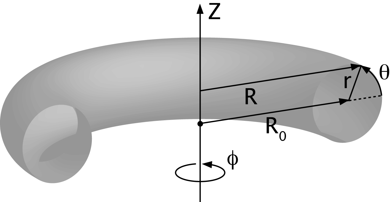
The magnetic field writes cf. [48]
where and stand the unit vectors of toroidal and poloidal coordinates system
with
Here is the quality factor, that is the number of toroidal winds of a magnetic line, corresponding to one poloidal wind. The magnetic field lines are either closed or dense on magnetic surface, depending whether the quality factor is rational, ( , are integers) or not. If is rational, the field line is closed otherwise the field line is dense on a magnetic surface. It is obvious that a field line on a magnetic surface with closes itself after traveling toroidal turns and poloidal turns.
In Cartesian coordinates, the magnetic field writes
Both the fields , leave invariant the function and therefore we have . We denote by the characteristic flow of . We have
implying that
| (33) |
In order to determine the evolution of the toroidal angle , we write
leading to
| (34) |
The differential equation (33) also writes
| (35) |
and thus we obtain
As , the poloidal angle is increasing and there is such that , . The number comes by the above equality that
and thus . By (33) and (34) we have , implying that
Therefore the magnetic lines wind times along the toroidal angle while doing one wind along the poloidal angle. As is left invariant by the flow , we have and thus if , saying that the characteristic flow is -periodic. Observe that
and therefore the magnetic field is divergence free. We are looking for angular vector fields. Motivated by (35), we consider
Since , we also have from (35) that and we take
Proposition 6.1
The vector fields are angular. The magnetic field
writes
with
Proof.
It is easily seen that the vector and are angular fields. For the decomposition of magnetic field , notice that, in the definition of , the gradients of the angles are understood as the continuous vector fields
and
By direct computations we have
and
and
Taking the scalar product with we obtain the coefficients in the decomposition of the magnetic field .
7 Convergence result
We concentrate now on the asymptotic behavior as of the family of weak solutions of the Vlasov-Poisson-Fokker-Planck system (1), (2), and (3) and we establish rigorously the connection to the fluid model (4), (5), and (6).
We are looking a model for the concentration , similar to the equation (4) of the limit concentration and we perform the balance of the relative entropy between and . As usual, these computations require the smoothness of the solution for the limit model. We justify the asymptotic behavior of when , provided that there is a smooth solution for the fluid model (4), (5), and (6). We do not concentrate on the well posedness of this fluid model, nevertheless we refer to Section 6.1 for some examples of smooth solutions. We are working with weak solutions .
The balance for the number of particles writes
| (36) |
We are using the balance momentum as well
| (37) |
which allows us to express the orthogonal component of
where we denote
and in the above computation, we have used that .
Observe that
and finally, thanks to (36), we obtain a similar model for , as in (4)
| (38) |
We are also looking for a equation, analogous to (5), in order to complete the evolution equation (38), involving the Lagrange multiplier . Considering the parallel component in the momentum balance (37), we obtain
Thanks to (5), the above equation also writes
| (39) |
We intend to estimate the modulated energy of with respect to by writing as
| (40) |
We introduce as well the modulated energy of with respect to , given by
Thanks to the free energy balance (13) and mass conservation of (1) one gets
| (41) | ||||
Thanks to Proposition 3.1 and combining (7), (41) leads to
| (42) |
The next task is to evaluate the time derivative of . Notice that for any smooth concentration , we can write
where . Clearly, we have
| (43) |
Proof.
By straightforward computations, we obtain
| (44) | ||||
where in the last integral we have used the contraint which allows us to deduce that
| (45) | ||||
Thanks to (43) again, the last integral in (7) writes easily
| (46) | ||||
Observe that
Coming back to (7), the modulated energy balance becomes
| (47) | ||||
where . In order to apply Gronwall lemma, we estimate the terms in the last integral of (7). Thanks to the formula
we obtain
where for any matrix , the notation stands for . Similarly, we have for some value to be precised later on
Since we have
Plugging the above computations in (7), the modulated energy balance becomes for
Taking and large enough, we obtain by Lemma 2.1 and (7), for some constant , ,
Applying Gronwall lemma, we deduce that for ,
The above inequality says that the particle density remains close to the Maxwellian with the same concentration, , and stays near , provided that analogous behaviour occur for the initial conditions. Therefore, we are ready to prove our main theorem.
Proof. (of Theorem 1.1)
We justify the convergence of toward in , the other convergences being obvious. We use the Csisár -Kullback inequality in order to control the norm by the relative entropy, cf. [32, 45]
for any non negative integrable functions . Applying two times the Csisár -Kullback inequality we obtain
In the same manner we perform the balance of the relative between two smooth solutions of the limit model.
Proposition 7.2
8 Example of smooth solutions for limit model
In this section we construct smooth solution for the limit model obtained in Section 6.1. We focus on the existence of the limit model
| (48) |
where stands for the Poisson electric potential which solves
| (49) |
Denoting the electric field derives from the potential . We supplement our model by the initial condition
| (50) |
where is a smooth function and belongs to . The external magnetic field we consider here . Notice that the vector field .
We follow the same arguments as in the well-posedness proof for the Vlasov-Poisson problem with an external magnetic field, as discussed in [18, 19]. Our goal is to obtain a priori bounds for the norm of and , not in the full space , but in . These bounds rely on estimating the fundamental solution of Laplace’s equation on . Therefore, we begin by investigating the Poisson equation for a given density in this domain and finding a fundamental solution for this purpose.
8.1 Fundamental solution of Laplace’s equation on
Consider a function satisfying
| (51) |
in the sense of distributions, where denotes the Dirac measure on giving unit mass to the point .
Lemma 8.1
Proof.
We have
| (52) |
where we have used the Poisson summation formula
Indeed, the is periodic with period , it can be represented as a Fourier series
where the Fourier coefficients are
On the other hand, as is periodic in of period , we also have
therefore
| (53) |
Comparing (52) and (53) yields the following linear elliptic equation in the whole space for any
| (54) |
A solution to (54) can be found by using the Fourier transform for linear equation. It is known that the solution to this equation is given in term of the Bessel potential as , cf. [38] where Thus, we have the solution formula
In the case , the equation (54) becomes the Laplace equation on . It is well known that the fundamental solution is given by . Finally, we obtain
Let us denote and . It is know that is a heat kernel on of the heat equation
while is a heat kernel on of
For a proof of this property, we refer to [29]. We define now . Then is the fundamental solution of heat equation on , that means
Thus, we have that the function in the fundamental solution for Laplace’s equation (51) is related to the previous solution of heat equation as
| (55) |
Remark 8.1
The heat kernel on can also be given by the heat kernel on the real line as follows
| (56) |
Indeed, the function since
where is Haar measure on , . Thus, the periodic function can be written in the form of the Fourier serie
where is the sequence of the Fourier coeffiecients which is given by
where is the Fourier transform of the function .
Since we need the bounds of the function and its derivatives in the following, we must to estimate the function and also the first and second derivates of from (55). We shall use the arguments in [50] to obtain the bound of . Firstly, using the formula (56), we can rewrite the function on as follows:
Lemma 8.2
For any and for any , we have
Proof.
Using the definition of , we have
which gives the claim, using .
Next, using Lemma 8.2, we obtain the following estimate
Lemma 8.3
For any and any , we have
| (57) |
Proof.
Using Lemma 8.2 and the fact that from we get the lower bound. Indeed, for any
For the upper bound, let us write
For any , using
Therefore
Together with implies the upper bound we wanted to prove.
We need the estimate of the function at .
Lemma 8.4
For any , we have
and
Consequently, there exist positive constants such that .
Proof.
Using Lemma 8.2 with gives . By formula (56) we have
Since is positive and decreasing, bounding a sum by an integral we get
hence . Moreover, we have . Finally, since , for any , we deduce that which gives . To finish Lemma, it remains to prove , for any . Indeed, we have
for some positive constants and .
Now, the following lemma provides estimates of and its derivatives on .
Lemma 8.5
Let be the heat kernel on . Then there exist constants and which can change from line to line such that
| (58) |
| (59) |
| (60) |
Proof.
Readers can find these results in [29], even when is replaced by more general compact manifold, cf. [57, 60]. We provide here the main lines of the proof.
For the bound (58), it is easily obtained from the consequence of Lemma 8.4 for . If , first using (56) yields
then (57) we have
| (61) |
Using the upper bound in (61) and Lemma 8.4 we deduce that
If , for some , it’s not hard to show from the previous inequality that there exist positive constants and such that . On the other hand, for any positive test function , since and , where is the heat kernel on , we deduce that we can choose the positive constants as above to obtain the previous estimate of as . Together, these arguments give us the upper bound of (58). Similarly, by using the lower bound in (61), we infer the lower bound in (58). Therefore, we obtain the estimate (58). Now, for the estimates (59) and (60), we apply Lemma in [57], which can be extended to the parabolic case, see Lemma in [57]
where is asolution of the heat equation in the domain , with for any fixed point .
In the next lemma, we provide estimates for the function and its derivatives using the relation (55) and the inequalities (58), (59) and (60).
Lemma 8.6
Let be the function on provided by Lemma 8.1. Then we have the following estimates
where denotes the second order derivative. Here, stands for a positive constant, which can vary in each estimate.
Proof.
We will first estimate . Thanks to (55) and (58), we deduce that
for some positive constant , where we have used that
| (62) |
see the proof of Lemma 8.12 in Appendix.
Next we estimate . Taking the derivative with respect to in the formula (55) we deduce that
A simple computation show that
and thanks to the estimates (58) and (59) we obtain
where . Using where for the first integral on the last line of the previous inequality, we deduce that
for some positive constant .
Finally, we estimate . By direct computation in (58), we have
Since
it implies that
Using the inequalities (58), (59) and (60) we deduce that
The estimates of the integrals and are performed as above. Thus we get
For the integral , we have that
Using again where , we obtain that , for some positive constant . Similarly for integral , we also have
Together, the estimations of , for any will provide us the estimate of .
8.2 Estimations for the electric field and its gradient on
We give now some estimates of the electric field which can be proved by treating the singular term in the fundamental solution as in, cf. [3] for the space domain and [43] for .
Lemma 8.7
Let be a positive concentration and belongs to . Then, there exists a constant such that the electric field satisfies the following estimate:
Proof.
For any , by the formula (63) we have
The first integral in the previous expression can be estimated as
For the second integral, we make a decomposition of in the following way
where
It is obviously that . Thus the last integral in the previous equality can be written
Thanks to Lemma 8.6, we deduce that
where we have used that . Combining these estimates, we obtain the desired result in Lemma.
Lemma 8.8
Let and . There exists a constant such that the gradient of the electric field satisfies the following estimates
where the notation stands for the positive part of .
Proof.
Observe that
because the functions and are periodic with respect to of period . We estimate now . In other cases, we can do the same. Taking the derivative in the variable of the above equality, we have
which implies that
The estimation of , see [3]. We estimate now . Let such that verify
Then we make a decomposition of in the following way
where
For the integral on , thanks to the integration by parts with respect to and noticing that the boundary of is , we get
| (64) |
Similarly, the integral on can be written as
| (65) |
For the integral on , since and then using the integration by parts, we obtain
| (66) |
Combining the equalities (8.2), (8.2) and (8.2) we deduce that
Thanks to Lemma 8.6, we will estimate the integrals , for any .
For the integral , using the estimate of we have
For the integral , using the estimate of we also get
Similarly for the integral and the integral , we obtain
Finally, together these estimates of , for any we obtain
Taking and which gives us the result of the lemma.
8.3 Local existence of smooth solutions
Let’s begin to establish strong solutions for the limit model. It is sufficient to construct a solution on some time interval , . We present only the main arguments, the other details being left to the reader. We assume that the initial condition satisfies the hypotheses
-
H1)
,
-
H2)
.
Solution integrated along the characteristics
A standard computation, we can rewrite the equation (48) as
| (67) |
For any smooth field , we consider the associated characteristics flow of this equation
| (70) |
where is the solution of the ODE, represents the time variable, is the initial time and is the initial position. is our initial condition. Notice that the vector field is also smooth and belongs to . Therefore, the characteristics in (70) are well defined for any and there are smooth with respect to . From (70), the equation (67) can be written as
The solution of the transport equation (67) is given by
| (71) |
Conservation law on a volume
We have the following conservation law
| (72) |
Indeed, we denote is the Jacobian matrix of with respect to at . The determinant of the Jacobian matrix is given by
Hence, we obtain
Integrating the equality (71) with respect to and then changing the variable to , we obtain
A priori estimates
The bound in of the solutions
We have the following bounds
| (73) |
| (74) | ||||
where we denote the constants and .
We will first prove (73). By the formular (71), for any we have
We then prove (74). By taking the derivative with respect to in the formula (71), we imply
We estimate now . Since
therefore it remains to estimate . Taking the derivative with respect to in (70), we deduce that
for some constant depending on . Thanks to Grönwall’s inequality, we have
| (75) |
which implies for anty that
Next we estimate the following norm
A straightforward computations and then using (75) yield
for some constant depending on . Combining these estimates yield
where we used the notation for a universal constant depending on .
The bound in of the solutions
| (76) |
| (77) |
where is the constant depending on . Now we will prove (77). By taking the derivative with respect to in (71), we have
Then, we integrate with respect to and change the variable to . Notice that the Jacobian formula is given by
therefore we deduce that
Thanks to (75) we obtain
where we use same the notation for a universal constant depending on .
Local existence of solutions
We define
where are two constants to be fixed later. Given an electric field in . We consider the solution by characteristic of the equation (67) on , corresponding to the electric field and denote by which is given by the formula (71). We construct the following map on , whose fixed point gives the solution of the system (67), (49) and (50) at least locally in time such solutions exist
| (78) |
We will prove that the map is left invariant on the set for a convenient choice of the constants and , then we want to establish an estimate like
| (79) |
for some constant , not depending on and . After that, the existence of the system (67), (49) and (50) immediately, based on the construction of an iterative method for .
Lemma 8.9
There exist positive constants , and such that .
Proof.
Let . Thanks to Lemma 8.7 and the formulas (73) and (76), we have
Here, we fix as a constant such that , and we choose , where is a universal constant. Hence, we obtain
The bound of norm for the density in (73) becomes
| (80) |
It remains to estimate . Thanks to Lemma 8.8, we need to estimate . By the formula (74) we have
Thus, together with (80) we deduce that
Here, we fix as a constant such that and we take . Therefore we obtain
Now we establish the inequality (79). Consider and and denote by and the solutions by characteristics of (67), (50) with the same initial data corresponding to the electric fields and , respectively. It is easily seen from Lemma 8.7 that
Notice that the constant is not depend on and .
Lemma 8.10
We have
for some positive constant , not depending on .
Proof.
Thanks to (71), we deduce that
where and denote the characteristic of (70) corresponding to the vector fields and . We estimate now the integral . Since
so we need to estimate . We claim that
| (81) |
for some constant depending on . Indeed, from the equations in (70) we imply that
Integrating between and we find
Notice that , since . Then, the Gronwall lemma allows us to conclude that (81) holds. Therefore we have
Next, we estimate the integral . We utilize the inequality , valid for any . Applying the same argument as in the estimate of , we obtain
Notice that, for the sake of simplicity, we use the same notation in the inequalities for both and standing for a universal constant depending on . Finally, we combine the estimate for the integrals and to derive the result.
Lemma 8.11
We have
for some positive constant , not depending on .
Proof.
Since and are the solutions of (67) therefore we deduce that
Multiplying this equation by , then integrating with respect to , we obtain
Using the inequality (77) and a straightforward estimations yield
for some positive constant depending only on . Integrating between and and thanks to the Gronwall lemma we obtain the desired result.
Based on these arguments and Proposition 7.2, we establish the following result
Appendix
Lemma 8.12
For any , we have
Proof.
Let us denote . It is easily seen that
For any , by taking the derivative with respect to , we obtain that
which yields
| (82) |
Observer that
and by changing the variable one gets
Substituting in (82), we have
which implies is independant of value of and thus , for any .
Acknowledgement
This work has been carried out within the framework of the EUROfusion Consortium, funded by the European Union via the Euratom Research and Training Programme (Grant Agreement No 101052200 — EUROfusion). Views and opinions expressed are however those of the author(s) only and do not necessarily reflect those of the European Union or the European Commission. Neither the European Union nor the European Commission can be held responsible for them.
References
- [1] N.B. Abdallah, R. El Hajj, Diffusion and guiding center approximation for particle transport in strong magnetic fields, Kinet. Relat. Models, 1 (2008), 331-354.
- [2] C.W. Bardos, F. Golse, Toan T. Nguyen, R. Sentis, The Maxwell–Boltzmann approximation for ion kinetic modeling, Physica D: Nonlinear Phenomena, 376-377 (2016), 94-107.
- [3] J. Batt, Global symmetric solutions of the initial value problem of stellar dynamics, J. Diff. Equations, 25(1977) 342-364.
- [4] F. Berthelin, A. Vasseur, From Kinetic Equations to Multidimensional Isentropic Gas Dynamics Before Shocks, SIAM Journal on Mathematical Analysis. 36(2005) 1807-1835.
- [5] L. L. Bonilla, J. A. Carrillo and J. Soler, Asymptotic behaviour of the initial boundary value problem for the three dimensional Vlasov–Poisson–Fokker–Planck system, SIAM J. Appl. Math. 57 (1997) 1343–1372.
- [6] M. Bostan, The Vlasov–Maxwell System with Strong Initial Magnetic Field: Guiding-Center Approximation. Multiscale Modeling & Simulation, 6 (2007) 1026-1058.
- [7] M. Bostan, T. Goudon, High-electric-field limit for the Vlasov-Maxwell-Fokker-Planck system. Annales de l’I.H.P. Analyse non linéaire, 25 (2008) 1221-1251.
- [8] N.N. Bogoliubov, and Y.A. Mitropolsky, Asymptotic Methods in the Theory of Non-linear Oscillations, Published by Gordon & Breach, New York, 1961.
- [9] M. Bostan, Transport equations with disparate advection fields. Application to the gyrkinetic models in plasma physics, Journal of Differential Equations, 249 (2010), 1620-1663.
- [10] M. Bostan, The Vlasov-Poisson system with strong external magnetic field. Finite Larmor radius regime, Asymptot. Anal., 61 (2009), 91-123.
- [11] M. Bostan, Collisional models for strongly magnetized plasmas. The gyrokinetic Fokker-Planck equation, Libertas Math, 30 (2010), 99-117.
- [12] M. Bostan, Gyrokinetic Vlasov Equation in Three Dimensional Setting. Second Order Approximation, Multiscale Modeling & Simulation, 8 (2010), 1923-1957.
- [13] M. Bostan, A. Finot, M. Haurray, The effective Vlasov-Poisson system for strongly magnetized plasma, C. R. Acad. Sci. Paris, Ser. I 354(2016) 771-777.
- [14] M. Bostan, A. Finot, The Effective Vlasov-Poisson System for the Finite Larmor Radius Regime, SIAM J. Multiscale Model. Simul., 14 (2016), 1238-1275.
- [15] M. Bostan, Transport of Charged Particles Under Fast Oscillating Magnetic Fields, SIAM Journal on Mathematical Analysis, 44 (2012) 1415-1447.
- [16] M. Bostan, High magnetic field equilibria for the Fokker-Planck-Landau equation, Ann. Inst. H. Poincaré Anal. Non Linéaire, Vol. 33 (2016) 899-931.
- [17] M. Bostan, Multi-scale analysis for linear first order PDEs. The finite Larmor radius regime, SIAM J. Math. Anal. 48 (2016) 2133-2188.
- [18] M. Bostan, Asymptotic Behavior for the Vlasov–Poisson Equations with Strong External Magnetic Field. Straight Magnetic Field Lines, SIAM Journal on Mathematical Analysis, 51 (2019).
- [19] M. Bostan, Asymptotic behavior for the Vlasov-Poisson equations with strong external curved magnetic field. Part I : well prepared initial conditions, hal.inria.fr/hal-02088870/.
- [20] M. Bostan, C. Caldini-Queiros, Finite Larmor radius approximation for collisional magnetic confinement. Part I: the linear Boltzmann equation, Quart. Appl. Math., Vol. LXXII, No. 2(2014) 323-345.
- [21] M. Bostan, C. Caldini-Queiros, Finite Larmor radius approximation for collisional magnetic confinement. Part II: the Fokker-Planck-Landau equation, Quart. Appl. Math., Vol. LXXII, No. 3 (2014) 513-548.
- [22] M. Bostan, I.M. Gamba, Impact of strong magnetic fields on collision mechanism for transport of charged particles, J. Stat. Phys., 148(2012), 856–895.
- [23] M. Bostan, A-T. Vu, Asymptotic behavior of the two-dimensional Vlasov-Poisson-Fokker-Planck equation with strong external magnetic field, Preprint.
- [24] F. Bouchut, Existence and uniqueness of a global smooth solution for the Vlasov-Poisson-Fokker-Planck system in three dimension, J. Funct. Anal. 111(1993) 239-258.
- [25] F. Bouchut, Smoothing effect for the nonliear Vlasov-Poisson-Fokker-Planck system, J. Differential Equations, 122(1995) 225-238.
- [26] F. Bouchut and J. Dolbeaut, On long asymptotics of the Vlasov–Fokker–Planck equa- tion and of the Vlasov–Poisson–Fokker–Planck system with Coulombic and Newtonian potentials, Differential Integ. Equations 8 (1995) 487–515.
- [27] Y. Brenier, Convergence of the Vlasov-Poisson system to the incompressible Euler equations, Comm. Paryial Differential Equations 25(2000) 737-754.
- [28] Y. Brenier, N. Mauser, M. Puel, Incompressible Euler and e-MHD scaling limits of the Vlasov-Maxwell system, Commun. Math. Sci. 1(2003) 437-447.
- [29] B. Carrillo, X. Pan, Qi S. Zhang, Decay and vanishing of some axially symmetric D-solutions of the Navier-Stokes equations, Journal of Functional Analysis, 279(2020).
- [30] J.-A. Carrillo, Y.-P. Choi, J. Jung, Quantifying the hydrodynamic limit of Vlasov-type equations with alignment and nonlocal forces, Math. Models and Methods Appl. Sci Vol. 31(2021) 327-408.
- [31] J.-A. Carrillo, J. Soler, On the initial value problem for the Vlasov-Poisson-Fokker-Planck system with initial data in spaces, Math. Methods Appl. Sci 18(1995) 825-839.
- [32] I. Csiszár , Information-type measures of difference of probability distributons and indirect observation, Studia Sci. Math. Hungar, 2(1967) 299-318.
- [33] S. Chandrasekhar, Brownian motion, dynamic friction and stellar dynamics, Rev. Mod. Physics 21(1949) 383-388.
- [34] Y.-P. Choi, and I.-J. Jeong, Global-in-time existence of weak solutions for Vlasov–Manev–Fokker–Planck system, Kinetic and Related Models 16(2023) 41-53.
- [35] P. Degond, Global existence of smooth solutions for the Vlasov-Fokker-Planck equation in 1 and 2 space dimension, Annales Scientifiques de l’ENS, Série 4, 19(1986) 519-542.
- [36] P. Degond, F. Filbet, On the Asymptotic Limit of the Three Dimensional Vlasov–Poisson System for Large Magnetic Field: Formal Derivation, Journal of Statistical Physics 165(2016), 765–784.
- [37] J.-L. Delcroix, A. Bers, Physiquue des plasmas, EDP Sciences 2000.
- [38] L.-C. Evans, Partial Differential Equations: Second Edition (Graduate Studies in Mathematics) 2nd Edition, American Mathematical Soc., 2010 - 749 pages.
- [39] E. Fénod, E. Sonnendücker, Long time behavior of two-dimensional Vlasov equation with strong external magnetic field, Math. Models Methods Appl. Sci. 10(2000) 539-553.
- [40] F. Golse, L. Saint-Raymond, The Vlasov-Poisson system with strong magnetic field, J. Math. Pures Appl. 78(1999) 791-817.
- [41] F. Golse, L. Saint-Raymond, The Vlasov-Poisson system with strong magnetic field in quasineutral regime, Math. Models Methods Appl. Sci., 13(2003) 661-714.
- [42] T. Goudon, P.-E. Jabin, A. Vasseur, Hydrodynamic limits for the Vlasov-Navier-Stokes equations. Part II: Fine particles regimes, Indiana Univ. Math. J. 53(2004) 1517-1536.
- [43] G. Rein, A.-D. Rendall, Global existence of classical solutions to the vlasov-poisson system in a three-dimensional, cosmological setting, Archive for Rational Mechanics and Analysis, 126(1994) 183–201.
- [44] M. Herda, L.M. Rodrigues, Anisotropic Boltzmann-Gibbs dynamics of strongly magnetized Vlasov-Fokker-Planck equations, Kinetic and Related Models, 2019.
- [45] S. Kullback, A lower bound for discrimination in information in terms of variation, IEEE TRans. Information Theory 4(1967) 126-127.
- [46] W. W. Lee, Gyrokinetic approach in particle simulation, Physics of Fluids, 26(1983), 556–562.
- [47] R. G. Littlejohn, Hamiltonian formulation of guiding center motion, Phys. Fluids, 24(1981), 1730–1749.
- [48] M. Lutz, Etude mathématique et numérique d’un modèle gyrocinétique incluant des effets électromagnétique pour la simulation d’un plasma de Tokamak, Thèse de Doctorat.
- [49] E. Miot, On the gyrokinetic limit for the two-dimensional Vlasov-Poisson system, arXiv:1603.04502.
- [50] P. Maheux, Notes on Heat Kernels on Infinite dimensional Torus. Lecture note.
- [51] C. Negulescu, Kinetic Modelling of Strongly Magnetized Tokamak Plasmas with Mass Disparate Particles. The Electron Boltzmann Relation, Multiscale Modeling & Simulation, 16(2018), 1732-1755.
- [52] B.O’Dwyer, H.D. Victory Jr., On classocal solutions of the Vlasov-Poisson-Fokker-Planck system, Indiana Univ. Math. J. 39(1990) 105-156.
- [53] M. Puel, L. Saint-Raymond, Quasineutral limit for the relativistic Vlasov-Maxwell system, Asymptot. Anal. 40(2004) 303-352.
- [54] G. Rein, J. Weckler, Generic global classical solutions of the Vlasov-Poisson-Fokker-Planck system in three dimensions, Diff. Equations 99(1992) 59-77.
- [55] L. Saint-Raymond, Control of large velocities in the two-dimensional gyro-kinetic approximation, J. Math. Pures Appl. 81(2002) 379-399.
- [56] L. Saint-Raymond, Convergence of solutions to the Boltzmann equation in the incompressible Euler lomit, Arch. Ration. Mech. Anal. 166(2003) 47-80.
- [57] G. Tian, Qi S. Zhang, Isoperimetric inequality under Kähler Ricci flow, American Journal of Mathematics, 136(2014), 1155-1173.
- [58] H.D. Victory Jr., On the existence of global weak solutions for the Vlasov-Poisson-Fokker-Planck system, J. Math. Anal. Appl. 160(1991) 525-555.
- [59] H.T. Yau, relative entropy and hydrodynamics of Ginzburg-Landau models, Lett. Math. Phys. 22(1991) 63-80.
- [60] Qi S. Zhang, A formula for backward and control problems of the heat equation, arxiv.org/abs/2005.08375.