Distillation of optical Fock-states using atom-cavity systems.

Abstract

Fock states are quantized states of electromagnetic waves with diverse applications in quantum optics and quantum communication. However, generation of arbitrary optical Fock states still remains elusive. Majority of Fock state generation proposals rely on precisely controlling the atom-cavity interactions and are experimentally challenging. We propose a scheme to distill an optical Fock state from a coherent state. A conditional phase flip (CPF) with arbitrary phase is implemented between the atom and light. The CPF along with the unitary rotations and measurements on the atoms enables us to distil required Fock-state. As an example, we show the distillation of Fock-sate $\ket{100}$.

I introduction

The second quantization of electromagnetic fields reveals the equivalence of light modes with harmonic oscillators Loudon (2003). The eigenstates of these oscillators are called the Fock states and they describe the number of photons present in a specific mode of a light field. Due to their highly non-classical nature, they are extremely useful in various areas such as quantum metrology, quantum key distribution (QKD) protocols, and quantum computation Kok et al. (2007); Ralph (2006). However, their quantum nature also makes it difficult to produce them. In existing experiments, optical Fock states are produced using parametric down-conversion and photon number detectors. These techniques have been shown to produce Fock states up to 5 photons Waks et al. (2006); Tiedau et al. (2019); Cooper et al. (2013); Brańczyk et al. (2010); Lingenfelter et al. (2021), however, it is still a challenging task to produce higher Fock states in the optical regime.

Atom-cavity systems have been widely studied for deterministic generation of optical Fock states, Fock states are created inside the cavity by controlling the interaction between atoms and cavities Brown et al. (2003); Xia et al. (2012); Law and Eberly (1996). However, this requires precise control which is limited by the coherence time of the system. As the number of photons increases, control becomes harder and the fidelity of generated Fock states decreases Uria et al. (2020), making it difficult to generate high photon number states.

In addition to controlling the dynamics of atom-cavity systems, schemes based on feedback mechanisms have also been proposed for the deterministic generation of Fock states Dotsenko et al. (2009); Geremia (2006) . These schemes involve using a controller to probe the cavity mode with weak measurements, which provide information about the cavity field. Based on the information obtained from these measurements, an actuator applies feedback to the cavity. By repeatedly measuring and applying feedback, the cavity state can be prepared in any desired state. This method has been experimentally verified using Rydberg atoms and superconducting cavities Sayrin et al. (2011).

Further, another method for Fock-state sorting has been demonstrated using chiral coupling of a two-level system to a waveguide. In this method, the light acquires a Fock-number-dependent delay, and the incident pulse is sorted temporally by its Fock numbers Mahmoodian et al. (2020); Yang et al. (2022).

In this article, we propose a protocol to distil Fock states from a coherent state. It is based on repeated reflection of light from the atom-cavity system. Unlike the existing protocols, this doesn’t require precise control or feedback mechanisms. Also the Fock states in this scheme are generated outside the cavity avoiding further extraction which can effect the statistics of the light.

In Sec. II we discuss the conditional phase flip (CPF) between the atom and the light mode and study effects of cavity-light detuning on the CPF. Then in Sec. III the atom-photon phase gate along with unitary rotations and measurements are used to distil a Fock-state from a coherent state. Finally we conclude by discussing possible implementations.

II Atom-photon gate

Atom-photon gates aim to create a CPF between an atom and a flying photon. Typically this is confined only to a phase of $\pi$ as this is sufficient to implement a general unitary operation on atom-photon and photon-photon systems. To obtain a conditional phase shift, we consider a three level atom with ground states $\ket{g}$ and $\ket{s}$, and an excited state $\ket{e}$ as shown in with two dipole allowed transitions ($\ket{e}\leftrightarrow\ket{g}$ and $\ket{e}\leftrightarrow\ket{s}$), see Fig. 1. Here, only one of them $(\ket{e}\leftrightarrow\ket{g})$ is coupled to the cavity mode. The Hamiltonian of such system can be written as

$$H=\hbar\omega_{c}a^{\dagger}a+\hbar\omega_{eg}\outerproduct{e}{e}+\hbar g(\sigma_{eg}\hat{a}+\sigma_{ge}\hat{a}^{\dagger}),$$ (1)

$\omega_{eg}~{}(\omega_{c})$ is the transition frequency for the atom (cavity), $g$ is the atom cavity coupling strength. $\sigma_{eg}=\outerproduct{e}{g}$ is the atomic operator and $\hat{a}$ is the cavity mode operator. Although we are considering a single two-level atom interacting with the cavity mode, following results can be extend to dark states in $N$ two-level systems and $N$ atoms under Rydberg blockade conditions Sun and Chen (2018); Hao et al. (2019).

On solving the Eq. (1) for the dynamics yields the following reflection coefficients $r_{(1,0)}=\hat{a}_{\text{in}}/\hat{a}_{\text{out}}$ (see Appendix. A for details)

$$r_{1}=1-\dfrac{2}{(1+4C)-\mathrm{i}\Delta}, r_{0}=1-\dfrac{2}{1-\mathrm{i}\Delta},$$ (2)

where $\hat{a}_{\text{in}}$ ($\hat{a}_{\text{out}}$) is the operator for the input (output) mode. $r_{1}$ is the reflection coefficient for the coupled transition. $r_{0}$ is the reflection coefficient for the decoupled transition (empty cavity) Collett and Gardiner (1984). $C=g^{2}/\kappa\gamma$ is the cooperativity. $\Delta=2\Delta_{c}/\kappa$, $\Delta_{c}=\omega_{c}-\omega_{L}$ with $\omega_{L}$ being the mean frequency of the input pulse. Now by assuming $C\gg 1$ gives $r_{1}\simeq 1$ and $r_{0}$ can be any phase $e^{\mathrm{i}\phi}$. For example, numerically solving $r_{0}$ for $\phi=\quantity{\pi/2,\pi/4,\pi/8,\pi/16}$ gives $\Delta=\quantity{-1,-2.4142,-5.0273,-10.1531}$.

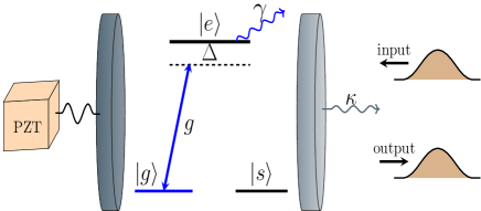
Figure 1: Atom cavity system for the CPF. A $\Lambda$-type atom with only $\ket{e}\leftrightarrow\ket{g}$ transition interacts with the cavity mode. $g$ and $\kappa$ are the coupling strength and the cavity decay rate of the cavity mode. $\Delta$ is detuning of the cavity mode with input light and the atom. The second mirror is attached to a Piezo actuator to tune the cavity resonant frequency.

On using Eq. (2) under strong atom-cavity coupling, the operation for the atom-cavity reflection can be written as (see Appendix. A)

$$\hat{\mathcal{D}}(\phi)=\outerproduct{g}{g}\otimes\mathcal{I}+\outerproduct{s}{s}\otimes\exp{\mathrm{i}\phi\hat{\Large n}}.$$ (3)

Note that cavity-light resonance $\Delta=0$ gives $r_{0}=-1$ ($\hat{\mathcal{D}}(\pi)$). This resonance condition has been exploited to generate atom-photon gates between atom and a single photon Reiserer and Rempe (2015). Further Eq. (3) transforms a coherent state into

$$\hat{\mathcal{D}}(\pi)[\psi_{a}\otimes\ket{\alpha}]=\dfrac{1}{\sqrt{2}}(\ket{g}\ket{\alpha}+\ket{s}\ket{-\alpha}),$$ (4)

where $\psi_{a}=\frac{1}{\sqrt{2}}(\ket{g}+\ket{s})$. Performing a $\small{\pi/2}$-rotation and a measurement on the atom, projects the light to a cat-state. This has been experimentally verified by trapping $\prescript{87}{}{\text{Rb}}$ to generate cat states with strength $\alpha=1.4$ Hacker et al. (2019).

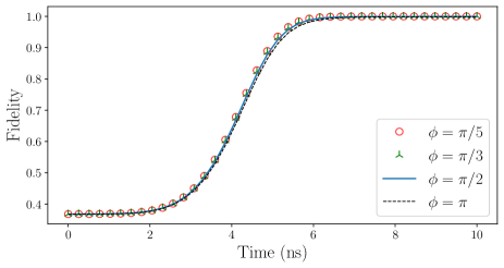
Figure 2: $\hat{\mathcal{D}}(\phi)$ operation attained from the steady state dynamics of atom-cavity system. We set $\quantity(g,\kappa,\gamma)=2\pi\times\quantity(16,~{}5,~{}0.05)~{}\text{GHz}$ for the numerical simulations.

The reflection coefficients are derived under the assumption that the atom-cavity system quickly attains a steady state. Though this is true on resonance Kiilerich and Mølmer (2020), detuning can effect the dynamics. In order to verify that steady states are attained even with detuning, we use input-output theory with quantum pulses to solve for the complete dynamics Kiilerich and Mølmer (2019, 2020). Upon reflection of light from the atom-cavity system, the following transformation is expected:

$$\psi_{a}\ket{\psi}_{\text{in}}\ket{0}_{\text{out}}\xrightarrow[\text{tion}]{\text{reflec}}\ket{0}_{\text{in}}\dfrac{\ket{g}\ket{\psi}_{\text{out}}+\ket{s}e^{\mathrm{i}\phi\Huge{\hat{n}}}\ket{\psi}_{\text{out}}}{\sqrt{2}}$$ (5)

and $\ket{\psi}_{\text{in,out}}=\sum_{n}C_{n}\ket{n}$ represents the quantum state of the input and output light modes.

In Fig. 2 we plot the fidelity for various phases. Here an input light is reflected from the atom-cavity system and the quantum state of the atom and the output light is numerically obtained. Then the fidelity is evaluated between the obtained and the expected output state Eq. (5) (see Appendix. B for more details). From the plot it is clear that reflection from atom-cavity yields the operation $\hat{\mathcal{D}}(\phi)$ on the output light mode and a steady is obtained even in the presence of cavity-light detuning.

III distillation of Fock states

We now use the phase shift operation $\hat{\mathcal{D}}(\phi)$, local unitary and measurement on atom to distil a Fock state. The protocol consists of the following steps:

1. To prepare the Fock state $\ket{\mathcal{A}}$, we start with a coherent state of amplitude $\alpha=\sqrt{\mathcal{A}}$.

2. Atom is prepared in the state $\psi_{a}=\frac{1}{\sqrt{2}}(\ket{g}+\ket{s})$

3. The light is reflected from the atom-cavity setup to perform $\hat{\mathcal{D}}(\phi)$.

4. A unitary rotation $U_{a}$ is performed on the atom Vitanov et al. (2017). $U_{a}[\theta]=\dfrac{1}{\sqrt{2}}\matrixquantity[e^{\mathrm{i}\theta}&1\\ 1&-e^{-\mathrm{i}\theta}],\matrixquantity{&\ket{g}\to\frac{1}{\sqrt{2}}(e^{\mathrm{i}\theta}\ket{g}+\ket{s})\\ &\ket{s}\to\frac{1}{\sqrt{2}}(\ket{g}-e^{-\mathrm{i}\theta}\ket{s})}$

5. Finally a measurement is performed on the atom Hacker et al. (2019).
   

Choosing $\alpha=\sqrt{\mathcal{A}}$ is not a stringent condition, this choice is based on the fact that coherent state has Poisson distribution with peak value at $\alpha^{2}$. The state of the “atom+output light” after step-$3$ can be written as

$$\Psi= \dfrac{1}{\sqrt{2}}\quantity[\psi_{l}\ket{g}+\exp{\mathrm{i}\phi\hat{n}}\psi_{l}\ket{s}],$$ (6)

where $\psi_{l}=\sum_{n}C_{n}\ket{n}$, is the state of light. Applying an appropriate $U_{a}[\theta]$, the atom-cavity state can always be cast in the form

$$\Psi=\sum_{k}C_{k}\ket{k}\ket{g}+\sum_{l}C_{l}\ket{l}\ket{s},$$ (7)

where $k\neq l$ and $\sum_{k}\absolutevalue{C_{k}}^{2}+\sum_{l}\absolutevalue{C_{l}}^{2}=1$ and measurement on the atom gives the photonic state

$$\psi_{l}=\sum_{k}C_{k}\ket{k}~{}\text{or}~{}\psi_{l}=\sum_{l}C_{l}\ket{l},$$ (8)

where $\sum_{k}\absolutevalue{C_{k}}^{2}$ and $\sum_{l}\absolutevalue{C_{l}}^{2}$ are the probabilities for the atomic measurements $\ket{g}$ and $\ket{s}$ .

By repeating the steps $2$ to $5$, it is possible to distil a general Fock state. We establish this by explicitly showing the distillation of the Fock state $\ket{100}$. The atom is initialized in the state $\psi_{a}$ and the input light in the coherent state $\ket{\alpha=10}$. The initial state of atom and light can be written as (see Appendix. C)

$$\Psi=\sum_{k=70}^{130}C_{k}\ket{k}\otimes\dfrac{1}{\sqrt{2}}(\ket{g}+\ket{s}),$$ (9)

where the coherent state is approximated as $\bm{\ket{\alpha=10}}\simeq\sum_{k=70}^{130}$ $C_{k}\ket{k}$. The explicit form $C_{k}$ is irrelevant to the distillation protocol and is only used to calculate measurement probabilities. Performing $\hat{\mathcal{D}}(\pi)$ on $\Psi$ yields

$$\Psi_{\pi}=\sum_{k=70}^{130}C_{k}e^{\mathrm{i}\pi\hat{n}}\ket{k}\ket{s}+\sum_{n=70}^{130}C_{k}\ket{k}\ket{g},$$ (10)

where $\Psi_{l}$ represents the state of output light after applying $\hat{\mathcal{D}}(l)$ operation. Note that $\hat{\mathcal{D}}(\pi)$ is obtained on resonance i.e. $\Delta=0$. Performing the atomic unitary $U_{a}[0]$ and measuring the atom in the state $\ket{g}$ removes the odd photons to give the even cat state Hacker et al. (2019)

$${\Psi_{\pi}}=\sum_{k=36}^{64}C_{2k}\ket{2k},$$ (11)

here the normalization is absorbed into the $C_{2k}$ i.e. $\sum_{k=36}^{64}\absolutevalue{C_{2k}}^{2}=1$ .

Preparing the atom in $\psi_{a}$ and reflecting the state ${\Psi}_{\pi}$ with $\hat{\mathcal{D}}(\pi/2)$ yields

$${\Psi_{\frac{\pi}{2}}}=\sum_{k=36}^{64}C_{2k}\quantity[(-1)^{k}\ket{s}+\ket{g}]\ket{2k},$$ (12)

performing $U_{a}[0]$ and a measurement in $\ket{g}$ projects the photonic state to $\Psi_{\pi/2}=\sum_{k=18}^{32}C_{4k}\ket{4k}$. Now reflecting the state ${\Psi}_{{\pi}/{2}}$ with $\hat{\mathcal{D}}(\pi/4)$ yields

$${\Psi_{\frac{\pi}{4}}}=\sum_{k=18}^{32}C_{4k}\quantity[(-1)^{k}\ket{s}+\ket{g}]\ket{4k},$$ (13)

applying $U_{a}[0]$ and a measurement in $\ket{s}$, projects the light state to $\Psi_{\pi/4}=\sum_{k=9}^{15}C_{8k+4}\ket{8k+4}.$ Reflecting ${\Psi}_{\pi/4}$ with $\hat{\mathcal{D}}(\pi/8)$ yields To cancel the extra factor of $\pi/2$, we perform $U_{a}[\pi/2]$. Now, measuring the atom in $\ket{g}$ projects the light state to Again reflecting $\Psi_{\pi/8}$ with $\hat{\mathcal{D}}(\pi/16)$ gives

$${\Psi_{\frac{\pi}{16}}}=\sum_{k=5}^{7}C_{16k+4}\quantity[(-1)^{k}e^{\frac{\mathrm{i}\pi}{4}}\ket{s}+\ket{g}]\ket{16k+4},$$ (14)

and finally performing $U_{a}[\pi/4]$ and measurement in $\ket{s}$ distils the Fock state $\ket{100}$.

Distilled Fock Nos.		$\phi$	$\theta$	$\mathcal{M}$	$\mathcal{P}$
$\quantity(k)_{k=70}^{130}$	70, 71…100…129, 130	$\pi$	0	$~{}\ket{g}~{}$
$\quantity(2k)_{k=36}^{64}$	70, 72…100…126, 128	$\pi/2$	0	$\ket{g}$	0.5
$\quantity(4k)_{k=18}^{32}$	72, 76…100…124, 128	$\pi/4$	0	$\ket{s}$	0.5
$\quantity(8k+4)_{k=9}^{15}$	76, 84…100…116, 124	$\pi/8$	$\pi/2$	$\ket{g}$	0.5
$\quantity(16k+4)_{k=5}^{7}$	84, 100, 116	$~{}\pi/16~{}$	$~{}\pi/4~{}$	$\ket{g}$	0.5
$\quantity(16k+4)_{k=6}$	100	-	-	-	0.64

Table 1: Distillation of Fock states. First column shows the sequence of distilled Fock numbers after each iteration. Second column shows the atom-cavity phase, $\hat{\mathcal{D}}(\phi)$. Other columns show the unitary operation $U_{a}[\theta]$ and the measurement ($\mathcal{M}$) on the atom. $\mathcal{P}$ is the probability of the outcome after each iteration. Note that atomic is prepared in $\psi_{a}$ after each iteration.

The distillation protocol discussed above is summarized in Table. 3 and it is clear that an arbitrary Fock state can be distilled by multiple iterations. We started with a coherent state with mean $\tiny(\expectationvalue{\hat{n}})$ and variance $\small(\expectationvalue{\hat{n}^{2}}-\expectationvalue{\hat{n}^{2}})$ of $\absolutevalue{\alpha}^{2}$. For high $\mathcal{A}$, the probability distribution can be approximated with a Gaussian and $\pm 3\sqrt{\mathcal{A}}$ covers the 0.997 of the total area of a Gaussian distribution (see Appendix. C). Also from the Table. 3, we notice that in each iteration, the total Fock numbers reduce by half. Thus the total number of iterations ($\mathcal{Q}$) required to distil a Fock state form the coherent state can be written as

$$6\sqrt{\mathcal{A}}=2^{\mathcal{Q}+1}~{}\Rightarrow~{}\mathcal{Q}=\lceil{\log_{2}{(6\expectationvalue{\Delta\hat{n}})}}\rceil-1,$$ (22)

where $\lceil{.}\rceil$ is the ceiling function and $\expectationvalue{\Delta\hat{n}}=[\expectationvalue{\hat{n}^{2}}-\expectationvalue{\hat{n}}^{2}]^{1/2}$ is the standard deviation of the coherent state. Although Eq. (22) is obtained assuming high coherent state amplitude, it works even for small amplitudes. Further squeezed coherent states with optimized squeezing Gerry et al. (2005) can be used to reduce the numbers of iterations to $\mathcal{Q}-1$ (see Appendix. C).

It is also interesting to note that a general CPF is not required and only phase shifts of the form $\phi=\pi/2^{n}$ are sufficient for the distillation protocol. Since every iteration requires an atomic measurement, the probability of success is $\sim 1/2^{M}$. Even though the probability of success decreases by increasing reflections, every iteration produces a highly non-classical state irrespective of the measurement outcome. Also the probability of success to generate a Fock state in the range $[\mathcal{A}-3\sqrt{\mathcal{A}},\,\mathcal{A}+3\sqrt{\mathcal{A}}]$ is unity.

Another special case of the distillation protocol is the deletion of prime numbered Fock states. Prime numbers by definition cannot be factored by any other number, this can be exploited to delete a Fock number from a given state. For example, reflecting the coherent state $\Psi$ (Eq. (9)) with phase $\hat{\mathcal{D}}(\pi/101)$, performing $U_{a}[0]$ and measuring the atom in $\ket{g}$ gives the photonic state $\Psi=\sum_{n=70}^{100}C_{n}\ket{n}+\sum_{n=102}^{130}C_{n}\ket{n}$.

IV Implementations and Discussion

Atom-cavity systems are used to implement a variety of protocols Reiserer and Rempe (2015). To implement this protocol, the cavity resonant frequency can be tuned to adjust the detuning $\Delta$. This can be achieved by attaching the cavity mirror to a peizo electric actuator Möhle et al. (2013). Besides tuning the cavity frequency, multiple atom-cavity systems with different detunings can also be considered. Waveguide QED is an effective approach to study such systems, where an array of atoms are trapped above waveguides to realize many atom-cavity systems on a single chipChang et al. (2018). Further, the amount of non-classicality of the output light increases after each iteration, which in-turn can make the quantum states strongly susceptible to transmission and photon losses Chuang et al. (1997). This discussion is beyond the scope of this article and will be studied separately.

Also, the coherent state pulses used in the distillation protocol typically have a narrow temporal widths and this can be used to realized highly non-classical bath. When the temporal width of the pulse is much narrower than the cavity linewidth, the pulse can effectively act as a bath for an atom-cavity system. This means that the first Markov approximation is satisfied, which assumes that the system-reservoir coupling strength is frequency independent Gardiner and Collett (1985).

V Acknowledgments

We would like to thank Dr Sandeep K. Goyal and Dr. G. Krishna Teja for their helpful discussions. Chanchal acknowledges the Council of Scientific and Industrial Research (CSIR), Government of India, for financial support through a research fellowship [Award No. 09/947(0106)/2019-EMR-I].

Appendix A Reflection coefficients for the atom-cavity system

Here we derive the reflection coefficients in the main text. The Hamiltonian of the atom cavity system is written as

$$H=\hbar\omega_{c}a^{\dagger}a+\hbar\omega_{a}\outerproduct{e}{e}+\hbar g(\sigma_{eg}a+\sigma_{ge}a^{\dagger}),$$ (23)

The dynamics of the system are governed by the Langevin equation and the input-output relation (Collett and Gardiner, 1984)

$$\begin{aligned} \derivative{\hat{\mathbf{x}}}{t}=&-\mathrm{i}\commutator{\hat{\mathbf{x}}}{H}-\Big{(}\commutator{\hat{\mathbf{x}}}{\hat{a}^{\dagger}}(-\dfrac{\kappa}{2}\hat{a}+\sqrt{\kappa}\hat{a}_{\text{out}})-\\ &\qquad(-\dfrac{\kappa}{2}\hat{a}^{\dagger}+\sqrt{\kappa}\hat{a}_{\text{out}})\commutator{\hat{\mathbf{x}}}{\hat{a}}\Big{)}\\ &-\Big{(}-\dfrac{\gamma}{2}\commutator{\hat{\mathbf{x}}}{\sigma_{eg}}\sigma_{ge}+\dfrac{\gamma}{2}\sigma_{eg}\commutator{\hat{\mathbf{x}}}{\sigma_{ge}}\Big{)}\end{aligned}$$ (24)

where $\hat{\mathbf{x}}$ is any operator of the atom-cavity system. $\gamma$ and $\kappa$ are the decay rates of atom and cavity. Note that the noise term for atomic decay are omitted because $\omega_{eg}$ is in the optical regime, hence the noise can be assumed to be vacuum. The dynamical equations are obtained as

$$\derivative{\hat{a}}{t}= -\mathrm{i}\omega_{c}\hat{a}-\mathrm{i}g\sigma_{ge}-\sqrt{\kappa}\hat{a}_{\text{out}}+\dfrac{\kappa}{2}\hat{a},$$ (25)

$$\derivative{\sigma_{ge}}{t}= -\mathrm{i}\omega_{a}\sigma_{ge}-\mathrm{i}g(\sigma_{gg}-\sigma_{ee})\hat{a}+\dfrac{\gamma}{2}\sigma_{ge},$$ (26)

Transforming $\matrixquantity[\hat{a},\sigma_{ge},\hat{a}_{\text{out}}]\to\matrixquantity[\hat{a},\sigma_{ge},\hat{a}_{\text{out}}]e^{-\mathrm{i}\omega_{L}t}$ gives

$$\derivative{\hat{a}}{t}= -\mathrm{i}\Delta_{c}\hat{a}-\mathrm{i}g\sigma_{ge}-\sqrt{\kappa}\hat{a}_{\text{out}}+\dfrac{\kappa}{2}\hat{a},$$ (27)

$$\derivative{\sigma_{ge}}{t}= -\mathrm{i}\Delta_{a}\sigma_{ge}-\mathrm{i}g(\sigma_{gg}-\sigma_{ee})\hat{a}+\dfrac{\gamma}{2}\sigma_{ge},$$ (28)

where $\Delta_{c}=\omega_{c}-\omega_{L}$ and $\Delta_{a}=\omega_{a}-\omega_{L}$. The input light is on resonance with the atomic transition ($\Delta_{a}=0$). Also atom is assumed to be weakly excited hence $\sigma_{gg}=1$. By setting $\partialderivative{\mathbf{x}}{t}=0$, the steady state solutions are obtained as

$$\hat{a}=\dfrac{-\sqrt{\kappa}}{\mathrm{i}\Delta_{c}-\kappa/2-\dfrac{g^{2}}{\gamma/2}}\hat{a}_{\text{out}}$$ (29)

On using the input-output relation $\hat{a}_{\text{out}}-\hat{a}_{\text{in}}=\sqrt{\kappa}\hat{a}$ yields

$$r_{1} =1-\dfrac{2}{1+4C-\mathrm{i}\Delta}, r_{0}=1-\dfrac{2}{1-\mathrm{i}\Delta},$$ (30)

where $\Delta=2\Delta_{c}/\kappa$ and the cooperativity $C={g^{2}}/{\kappa\gamma}$. The reflection coefficient for the non-interacting transition ($r_{0}$) is obtained using $C=0$. On using Eq. (30) an input state

$$\Psi_{\text{in}}=(c_{g}\ket{g}+c_{s}\ket{s})\otimes\sum_{n}c_{n}\dfrac{(\hat{a}_{\text{in}}^{\dagger})^{n}}{\sqrt{n!}}\ket{0}$$ (31)

upon reflection is transformed as follows:

$$\Psi_{\text{{out}}}=\quantity(c_{g}\ket{g}r_{1}^{\hat{n}}+c_{s}\ket{s}r_{0}^{\hat{n}})\otimes\sum_{n}c_{n}\ket{n},$$ (32)

here $\absolutevalue{c_{g}}^{2}+\absolutevalue{c_{s}}^{2}=1$ and $\absolutevalue{c_{n}}^{2}=1$. Form the Eq. (32) the transformation for general input state can be written as

$$\hat{\mathcal{D}}(\phi)=\outerproduct{g}{g}\otimes(r_{1})^{\hat{n}}+\outerproduct{s}{s}\otimes(r_{0})^{\hat{n}},$$ (33)

with $r_{1}\simeq 1$ and $r_{0}=e^{\mathrm{i}\phi}$ gives the Eq. (3).

$\Delta$	$e^{\mathrm{i}\phi}$	$r_{1}$
-1	$e^{\mathrm{i}\pi/2}$	$0.998+2\times 10^{-6}\mathrm{i}$
-2.41421	$e^{\mathrm{i}\pi/4}$	$0.998+4.8\times 10^{-6}\mathrm{i}$
-5.02734	$e^{\mathrm{i}\pi/8}$	$0.998+10^{-5}\mathrm{i}$
-10.15317	$e^{\mathrm{i}\pi/16}$	$0.998+2.02\times 10^{-5}\mathrm{i}$
-20.35547	$e^{\mathrm{i}\pi/32}$	$0.998+4.06\times 10^{-5}\mathrm{i}$

Table 2: Numerical solutions for reflection coefficients, here the cooperativity $C=250$. $\Delta$ represents the detuning required for $r_{0}=e^{\mathrm{i}\phi}$. We notice that $r_{1}\simeq 1$ .

Appendix B Verification of general phase

Here we discuss the verification of the general phase as described in Eq. (3). For this, we use the general input-output theory with quantum pulses Kiilerich and Mølmer (2019, 2020). It is based on density matrix formalism where the input and output pulses are replaced by virtual cavities coupled to the quantum system. This formalism explicitly incorporates the information of the pulse shapes and quantum states of the input and output pulses. The Hamiltonian governing the dynamics of the virtual cavities and the quantum system are given by

$$\begin{split}\hat{H_{\rm eff}}=\hat{H}_{s}+&\dfrac{\mathrm{i}}{2}\sqrt{\kappa}\quantity[g_{u}(t)\hat{a}^{\dagger}_{u}\hat{a}+g_{v}^{*}(t)\hat{a}^{\dagger}\hat{a}_{v}]\\ +&\quantity[g_{u}(t)g_{v}^{*}(t)\hat{a}_{u}^{\dagger}\hat{a}_{v}-h.c.],\end{split}$$ (40)

where $H_{s}$ denotes the system Hamiltonian given in Eq. (1) and $\hat{a}$ is the system cavity operator. $\hat{a}_{u}$ and $\hat{a}_{v}$ represent the input and output virtual cavity field operators with the corresponding time-dependent coupling strengths $g_{u}(t)$ and $g_{v}(t)$, respectively.

The time-dependent coupling strengths of these virtual cavities are chosen such that the input virtual cavity releases an input field with the required pulse shape $u(t)$, while the output virtual cavity acquires the output field mode with pulse shape $v(t)$. The relation between time profiles and coupling strengths is given by

$$g_{u}(t)=\dfrac{u^{*}(t)}{\sqrt{1-\int_{0}^{t}\absolutevalue{u^{\prime}(t)}^{2}dt^{\prime}}}, g_{v}(t)=-\dfrac{v^{*}(t)}{\sqrt{\int_{0}^{t}\absolutevalue{v^{\prime}(t)}^{2}dt^{\prime}}}.$$ (41)

The dynamics of the system are obtained by the solving the following Lindblad master equation

$$\derivative{\rho_{usv}}{t}=\dfrac{1}{\mathrm{i}\hbar}\commutator{\hat{H}}{\rho_{usv}}+\mathcal{D}[\hat{L}_{\rm eff}]\rho_{us},$$ (42)

where $\rho_{usv}$ is the density matrix of the full system including the input-virtual cavity, atom-cavity system and output-virtual cavity and $\mathcal{D}[\hat{L}_{\rm eff}]$ represents the time-dependent Lindblad dissipator with

$$\hat{L}_{\rm eff}(t)=\sqrt{\kappa}\hat{c}+g^{*}_{u}(t)\hat{a}_{u}+g^{*}_{v}(t)\hat{a}_{v}.$$ (43)

The output field mode can be obtained by considering only the input virtual cavity attached with the system with the Hamiltonian given by Kiilerich and Mølmer (2019)

$$\hat{H_{\rm 0}}=\hat{H}_{s}+\dfrac{\mathrm{i}}{2}\quantity[\sqrt{\kappa}g_{u}(t)\hat{a}^{\dagger}_{u}\hat{a}-\sqrt{\kappa}g^{*}_{u}(t)\hat{a}_{u}\hat{a}^{\dagger}],$$ (44)

along with the damping term given by the Lindblad operator

$$\hat{L_{0}}(t)=\sqrt{\kappa}\hat{c}+g^{*}_{u}(t)\hat{a}_{u}$$ (45)

The prominent output field modes along with the amount of excitation carried by them can be obtained by calculating the eigenmode decompostion of the following two-time correlation function Kiilerich and Mølmer (2020)

$$g^{(1)}(t,t^{\prime})=\expectationvalue{[\hat{L}_{0}(t)]^{\dagger}\hat{L}_{0}(t^{\prime})}\equiv\sum_{i}n_{i}v_{i}(t)$$ (46)

Using this, we can solve the master equation for the full system given in Eq. (42) and calculate the fidelity with time for state given in Eq. (3).

Appendix C Distillation using squeezed coherent states (SCS)

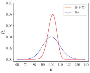
(a)

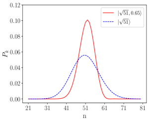
(b)

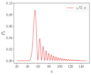
(c)

Figure 3: 3(a) and 3(b): Number squeezing for the SCS. $\ket{\alpha,r}$ and $\ket{\alpha}$ represents the SCS and the coherent state. An optimal squeezing can result in quantum states which are similar to a coherent state but with reduced variance. Due to the reduced variance SCS can be useful in minimizing iterations. 3(c) The effect of photon number oscillations for higher squeezing.

Distilled Fock No.	$\phi$	$\theta$	$\mathcal{M}$
36, 37…51 …65, 66	$\pi$	0	$\ket{s}$
37, 39…51 …63, 65	$\pi/2$	$\pi/2$	$\ket{s}$
39, 43…51 …59, 63	$\pi/4$	$3\pi/4$	$\ket{g}$
43, 51, 59	$\pi/8$	$3\pi/8$	$\ket{g}$
51	-	-

Distilled Fock Nos.	$\phi$	$\theta$	$\mathcal{M}$
85, 86…100…114, 115	$\pi$	0	$\ket{g}$
86, 88…100…112, 114	$\pi/2$	0	$\ket{g}$
88, 92…100…108, 118	$\pi/4$	0	$\ket{s}$
92, 100, 108	$\pi/8$	$\pi/2$	$\ket{g}$
100	-	-	-

Table 3: Distillation of the Fock states $\ket{51}$ and $\ket{100}$. First column shows the distilled Fock numbers after each iteration. Second column shows the atom-cavity phase, $\mathcal{D}(\phi)$. Other columns show the unitary operation $U_{a}[\theta]$ and the measurement ($\mathcal{M}$) on the atom.

In the main draft, we demonstrated distillation utilizing coherent states. It was evident that the number of iterations required depends on the Fock distribution. However, using squeezed coherent states (SCS) with squeezing can narrow the Fock distribution, potentially leading to a reduction in the required number of iterations. Here, we provide two examples using SCS and compare them with coherent states. These techniques can be applied for a general SCS. First we define the mean and variance of a quantum light

$$\expectationvalue{\hat{a}^{\dagger}\hat{a}}\equiv\expectationvalue{\hat{n}}, \expectationvalue{(\Delta\hat{n})^{2}}\equiv\expectationvalue{\hat{n}^{2}}-\expectationvalue{\hat{n}}^{2},$$ (59)

$$Q=\dfrac{\expectationvalue{(\Delta\hat{n})^{2}}-\expectationvalue{\hat{n}}}{\expectationvalue{\hat{n}}},$$ (60)

When $Q<0$ ($Q>0$), the light mode is said to obey sub (super) Poissonian statistics. The coherent state is written as

$$\ket{\alpha}=e^{-\dfrac{\absolutevalue{\alpha}^{2}}{2}}\sum_{k=0}^{\infty}\dfrac{\alpha^{k}}{\sqrt{k!}}\ket{k}, P_{k}=e^{-\expectationvalue{\hat{n}}}\dfrac{\expectationvalue{\hat{n}}^{k}}{k!},$$ (61)

where $P(k)$ is the probability for the $k^{\text{th}}$-Fock state and $\expectationvalue{\hat{n}}=\expectationvalue{(\Delta\hat{n})^{2}}=\absolutevalue{\alpha}^{2}$. For higher amplitudes $P(k)$ can be approximated with a Gaussian, further three standards are expected to include all the statistics

$$\sum_{n=0}^{\infty}P_{k}\approx\sum_{\expectationvalue{\hat{n}}-3\expectationvalue{\Delta\hat{n}}}^{\expectationvalue{\hat{n}}+3\expectationvalue{\Delta\hat{n}}}{P_{k}}=0.997.$$ (62)

A general SCS is written as Gerry et al. (2005)

$$\ket{\alpha,\xi}=\hat{\mathcal{D}}(\alpha^{\prime})\hat{\mathcal{S}}({\xi})\ket{0}$$ (63)

where $\xi=re^{\mathrm{i}\theta}$, $\alpha^{\prime}=\alpha e^{\mathrm{i}\phi}$ and $\phi=\theta/2$ . $\hat{\mathcal{D}}(\alpha^{\prime})$ is the displacement operator and $\hat{\mathcal{S}}(r)$ is the squeezing operator. The probability distribution, variance and the mean are obtained as Gerry et al. (2005)

$$\absolutevalue{\innerproduct{n}{\alpha^{\prime},\xi}}^{2}\equiv P^{\text{sq}}_{k}= ~{}\dfrac{(\frac{1}{2}\tanh r)^{k}}{k!\cosh r}~{}e^{-\alpha^{2}(1+\tanh r)}$$ (64)

$$\qquad\absolutevalue{H_{k}\quantity[\dfrac{{\alpha}e^{r}}{\sqrt{\sinh{2r}}}]}^{2},$$

$$\expectationvalue{(\Delta\hat{n})^{2}}= ~{}\alpha^{2}e^{-2r}+2\sinh^{2}r\cosh^{2}r,$$ (65)

$$\expectationvalue{\hat{n}}= ~{}\alpha^{2}+\sinh^{2}r,$$ (66)

where $H_{k}$ represents the $k^{\text{th}}$ order Hermite polynomial. with large coherent part ($\alpha\gg\sinh r$) and sub-Poissonian statistics $\expectationvalue{(\Delta\hat{n})^{2}}<\expectationvalue{\hat{n}}$, a SCS can give raise to the non-classical effect of number squeezing (see Fig. 3)

Similar to the coherent state (Eq. (62)) the SCS $\ket{10,0.75}$ and $\ket{\sqrt{51},0.65}$ are numerically verified to saitisfy

$$\sum_{n=0}^{\infty}P_{k}^{\text{sq}}\approx\sum_{\expectationvalue{\hat{n}}-3\expectationvalue{\Delta\hat{n}}}^{\expectationvalue{\hat{n}}+3\expectationvalue{\Delta\hat{n}}}P_{k}^{\text{sq}}=0.9995.$$ (67)

Using Eq. (22) and Eq. (65), we can determine that four iterations are required to distill Fock states $\quantity{\ket{51},\ket{100}}$ form $\quantity{\ket{10,0.75},\ket{\sqrt{51},0.65}}$, while using coherent states $\quantity{\ket{10},\ket{\sqrt{51}}}$ requires five iterations. We performed the distillation protocol to verify this, see Table. 3. By optimizing over the squeezing parameter, we can reduce the number of iterations by one. However, increasing the squeezing beyond a certain level may cause oscillations in the photon number distribution and require more iterations Gerry et al. (2005), as shown in Fig. 3(c).

References

- Loudon (2003) R. Loudon, The Quantum Theory of Light, Oxford science publications (Oxford University Press, 2003).
- Kok et al. (2007) P. Kok, W. J. Munro, K. Nemoto, T. C. Ralph, J. P. Dowling, and G. J. Milburn, Rev. Mod. Phys. 79, 135 (2007).
- Ralph (2006) T. Ralph, Reports on Progress in Physics 69, 853 (2006).
- Waks et al. (2006) E. Waks, E. Diamanti, and Y. Yamamoto, New Journal of Physics 8, 4 (2006).
- Tiedau et al. (2019) J. Tiedau, T. J. Bartley, G. Harder, A. E. Lita, S. W. Nam, T. Gerrits, and C. Silberhorn, Phys. Rev. A 100, 041802 (2019).
- Cooper et al. (2013) M. Cooper, L. J. Wright, C. Söller, and B. J. Smith, Optics express 21, 5309 (2013).
- Brańczyk et al. (2010) A. M. Brańczyk, T. Ralph, W. Helwig, and C. Silberhorn, New Journal of Physics 12, 063001 (2010).
- Lingenfelter et al. (2021) A. Lingenfelter, D. Roberts, and A. A. Clerk, Science Advances 7, 10.1126/sciadv.abj1916 (2021).
- Brown et al. (2003) K. R. Brown, K. M. Dani, D. M. Stamper-Kurn, and K. B. Whaley, Phys. Rev. A 67, 043818 (2003).
- Xia et al. (2012) K. Xia, G. K. Brennen, D. Ellinas, and J. Twamley, Optics Express 20, 27198 (2012).
- Law and Eberly (1996) C. K. Law and J. H. Eberly, Phys. Rev. Lett. 76, 1055 (1996).
- Uria et al. (2020) M. Uria, P. Solano, and C. Hermann-Avigliano, Phys. Rev. Lett. 125, 093603 (2020).
- Dotsenko et al. (2009) I. Dotsenko, M. Mirrahimi, M. Brune, S. Haroche, J.-M. Raimond, and P. Rouchon, Phys. Rev. A 80, 013805 (2009).
- Geremia (2006) J. Geremia, Phys. Rev. Lett. 97, 073601 (2006).
- Sayrin et al. (2011) C. Sayrin, I. Dotsenko, X. Zhou, B. Peaudecerf, T. Rybarczyk, S. Gleyzes, P. Rouchon, M. Mirrahimi, H. Amini, M. Brune, et al., Nature 477, 73 (2011).
- Mahmoodian et al. (2020) S. Mahmoodian, G. Calajó, D. E. Chang, K. Hammerer, and A. S. Sørensen, Phys. Rev. X 10, 031011 (2020).
- Yang et al. (2022) F. Yang, M. M. Lund, T. Pohl, P. Lodahl, and K. Mølmer, Phys. Rev. Lett. 128, 213603 (2022).
- Sun and Chen (2018) Y. Sun and P.-X. Chen, Optica 5, 1492 (2018).
- Hao et al. (2019) Y. Hao, G. Lin, X. Lin, Y. Niu, and S. Gong, Scientific reports 9, 4723 (2019).
- Collett and Gardiner (1984) M. J. Collett and C. W. Gardiner, Phys. Rev. A 30, 1386 (1984).
- Reiserer and Rempe (2015) A. Reiserer and G. Rempe, Rev. Mod. Phys. 87, 1379 (2015).
- Hacker et al. (2019) B. Hacker, S. Welte, S. Daiss, A. Shaukat, S. Ritter, L. Li, and G. Rempe, Nature Photonics 13, 110 (2019).
- Kiilerich and Mølmer (2020) A. H. Kiilerich and K. Mølmer, Phys. Rev. A 102, 023717 (2020).
- Kiilerich and Mølmer (2019) A. H. Kiilerich and K. Mølmer, Phys. Rev. Lett. 123, 123604 (2019).
- Vitanov et al. (2017) N. V. Vitanov, A. A. Rangelov, B. W. Shore, and K. Bergmann, Rev. Mod. Phys. 89, 015006 (2017).
- Gerry et al. (2005) C. Gerry, P. Knight, and P. L. Knight, Introductory quantum optics (Cambridge university press, 2005) Chap. 7.
- Möhle et al. (2013) K. Möhle, E. V. Kovalchuk, K. Döringshoff, M. Nagel, and A. Peters, Applied Physics B 111, 223 (2013).
- Chang et al. (2018) D. E. Chang, J. S. Douglas, A. González-Tudela, C.-L. Hung, and H. J. Kimble, Rev. Mod. Phys. 90, 031002 (2018).
- Chuang et al. (1997) I. L. Chuang, D. W. Leung, and Y. Yamamoto, Phys. Rev. A 56, 1114 (1997).
- Gardiner and Collett (1985) C. W. Gardiner and M. J. Collett, Phys. Rev. A 31, 3761 (1985).