Quantitative Measurement of Cyber Resilience: Modeling and Experimentation

Abstract

Cyber resilience is the ability of a system to resist and recover from a cyber attack, thereby restoring the system’s functionality. Effective design and development of a cyber resilient system requires experimental methods and tools for quantitative measuring of cyber resilience. This paper describes an experimental method and test bed for obtaining resilience-relevant data as a system (in our case – a truck) traverses its route, in repeatable, systematic experiments. We model a truck equipped with an autonomous cyber-defense system and which also includes inherent physical resilience features. When attacked by malware, this ensemble of cyber-physical features (i.e., “bonware”) strives to resist and recover from the performance degradation caused by the malware’s attack. We propose parsimonious mathematical models to aid in quantifying systems’ resilience to cyber attacks. Using the models, we identify quantitative characteristics obtainable from experimental data, and show that these characteristics can serve as useful quantitative measures of cyber resilience.

I Introduction

Resilience continues to gain attention as a key property of cyber and cyber-physical systems, for the purposes of cyber defense. Although definitions vary, it is generally agreed that cyber resilience refers to the ability of a system to resist and recover from a cyber compromise that degrades the performance of the system [1, 2, 3]. One way to conceptualize resilience is as the ability of a system to absorb stress elastically and return to the original functionality once the stress is removed or nullified [4]. Resilience should not be conflated with risk or security [5].

To make the discussion more concrete, consider the example of a truck which attempts to complete its goal of delivering heavy cargo. The cyber adversary’s malware successfully gains access to the Controller Area Network (CAN bus) of the truck [6]. Then, the malware executes cyber attacks by sending a combination of messages intended to degrade the truck’s performance and diminish its ability to complete its goal. We assume that the malware is at least partly successful, and the truck indeed begins to experience a degradation of its goal-relevant performance.

At this point, we expect the truck’s resilience-relevant elements to resist the degradation and then to recover its performance to a satisfactory level, within an acceptably short time period. These “resilience-relevant elements” might be of several kinds. First, because the truck is a cyber-physical system, certain physical characteristics of the truck’s mechanisms will provide a degree of resilience. For example, the cooling system of the truck will exhibit a significant resistance to overheating even if the malware succeeds in misrepresenting the temperature sensors data. Second, appropriate defensive software residing on the truck continually monitors and analyzes the information passing through the CAN bus [7]. When the situation appears suspicious, it may take actions such as blocking or correcting potentially malicious messages. Third, it is possible that a remote monitoring center, staffed with experienced human cyber defenders, will detect a cyber compromise and will provide corrective actions remotely [8].

For the purposes of this paper, we assume that the remote monitoring and resilience via external intervention is impossible [9]. This may be the case if the truck cannot use radio communications due to environmental constraints (e.g., operating in a remote mountainous area), or if the malware spoofs or blocks communication channels of the truck. Therefore, in this paper we assume that resilience is provided by the first two classes of resilience-relevant elements. Here, by analogy with malware, we call these “bonware” – a combination of physical and cyber features of the truck that serve to resist and recover from a cyber compromise.

A key challenge in the field of cyber resilience is quantifying or measuring resilience. Indeed, no engineering discipline achieved significant maturity without being able to measure the properties of phenomena relevant to the discipline [8]. Developers of systems like a truck must be able to quantify the resilience of the truck under development in order to know whether the features they introduce in the truck improve its cyber resilience, or make it worse. Similarly, buyers of the truck need to know how to specify quantitatively the resilience of the truck, and how to test resilience quantitatively in order to determine whether the product meets their specifications.

In this paper, we report results of a project called Quantitative Measurement of Cyber Resilience (QMoCR) in which our research team seeks to identify quantitative characteristics of systems’ responses to cyber compromises that can be derived from repeatable, systematic experiments. Briefly, we have constructed a test-bed in which a surrogate truck is subjected to controlled cyber attacks produced by malware. The truck is equipped with an autonomous cyber-defense system [7, 9] and also has some inherent physical resilience features. This ensemble of cyber-physical features (i.e., bonware) strives to resist and recover from the performance degradation caused by the malware’s attack. The test bed is instrumented in such a way that we can measure observable manifestations of this contest between the malware and bonware, especially the performance parameters of the truck.

The remainder of the paper is organized as follows. In the next section, we briefly describe prior work related to quantification of cyber resilience. In the following section, we propose a class of parsimonious models in which effects of both malware and bonware are approximated as deterministic, continuous differentiable variables, and we explore several variations of such models. In addition, we discuss how parameters of such models can be obtained from experimental data and whether these parameters might be considered quantitative characteristics (i.e., measurements) of the bonware’s cyber resilience. In the next section, we introduce the experimental approach we used to obtain resiliency-relevant data; we describe various components of the overall experimental apparatus and the process of performing experiments. The ensuing sections illustrate the experimentation and analysis using a case study, discuss the experimental results, and offer conclusions.

II Prior work

A growing body of literature explores quantification of resilience in general and cyber resilience in particular. Approximately, the literature can be divided into two categories: (1) qualitative assessments of a system (actually existing or its design) by subject matter experts (SMEs) [10, 11] and (2) quantitative measurements based on empirical or experimental observations of how a system (or its high-fidelity model) responds to a cyber compromise [3, 12]. In the first category, a well-cited example is the approach called the cyber-resilience matrix [13]. In this approach, a system is considered as spanning four domains: (1) physical (i.e., the physical resources of the system, and the design, capabilities, features and characteristics of those resources); (2) informational (i.e., the system’s availability, storage, and use of information); (3) cognitive (i.e., the ways in which informational and physical resources are used to comprehend the situation and make pertinent decisions); and (4) social (i.e., structure, relations, and communications of social nature within and around the system). For each of these domains of the system, SMEs are asked to assess, and to express in metrics, the extent to which the system exhibits the ability to (1) plan and prepare for an adverse cyber incident; (2) absorb the impact of the adverse cyber incident; (3) recover from the effects of the adverse cyber incident; and (4) adapt to the ramifications of the adverse cyber incident. In this way, the approach defines a 4-by-4 matrix that serves as a framework for structured assessments by SMEs.

Another example within the same category (i.e., qualitative assessments of a system by SMEs) is a recent, elaborate approach proposed by [14]. The approach is called Framework for Operational Resilience in Engineering and System Test (FOREST), and a key methodology within FOREST is called Testable Resilience Efficacy Elements (TREE). For a given system or subsystem, the methodology requires SMEs to assess, among others, how well the resilience solution is able to (1) sense or discover a successful cyber-attack; (2) identify the part of the system that has been successfully attacked; (3) reconfigure the system in order to mitigate and contain the consequences of the attack. Assessment may include tests of the system, although the methodology does not prescribe the tests.

Undoubtedly, such methodologies can be valuable in finding opportunities in improvements of cyber-resilience in a system that is either at the design stage or is already constructed. Still, these are essentially qualitative assessments, not quantitative measurements derived from an experiment.

In the second category (i.e., quantitative measurements based on empirical or experimental observations of how a system, or its high-fidelity model, responds to a cyber compromise), most approaches tend to revolve around a common idea we call here the area under the curve (AUC) method [15, 16].

The general idea is depicted in Figure 1. The functionality is plotted over time $t$. At time $t=t_{0},$ a cyber attack begins to degrade the functionality of the system, as compared to the normal level of functionality. The system resists the effects of the cyber attack, and eventually stabilizes the functionality at a reduced level. At $t=t_{1},$ the system resilience mechanisms begin to overcome the effect of the attack and eventually recover the functionality to a normal level. The area under the curve (AUC) reflects the degree of resilience – the closer AUC is to its normal level, the higher is the system’s resilience.

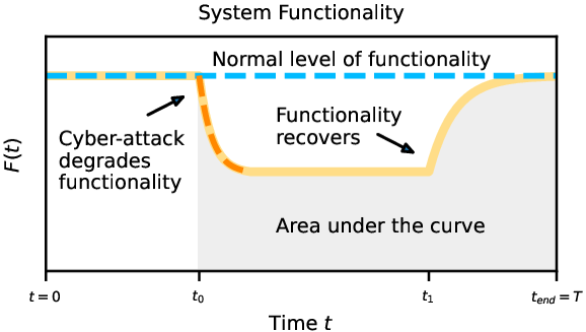
Figure 1: The functionality $F(t)$ is plotted over time $t$. At time $t=t_{0},$ a cyber attack begins to degrade the functionality of the system, as compared to the normal level of functionality. The system resists the effects of the cyber attack, and eventually stabilizes the functionality at a reduced level. At $t=t_{1},$ the system resilience mechanisms begin to overcome the effect of the attack and eventually recover the functionality to a normal level. The area under the curve (AUC) reflects the degree of resilience – the closer AUC is to its normal level, the higher is the system’s resilience.

In an experiment/test, a system engages in the performance of a representative goal, and then is subjected to an ensemble or sequence of representative cyber attacks. A goal-relevant quantitative functionality of the system is observed and recorded. The resulting average functionality, divided by normal functionality, can be used as a measure of resilience.

However, AUC-based resilience measures are inherently cumulative, aggregate measures, and do not tell us much about the underlying processes. For example, is it possible to quantify the resilience effectiveness of the bonware of the given system? Similarly, is it possible to quantify the effectiveness of malware? In addition, is it possible to gain insights into how these values of effectiveness vary over time during an incident? We will offer steps toward answering such questions in addition to evaluating the AUC as a resilience measure.

With respect to experimental approaches, much of the early experimental work on the cybersecurity of automobiles used actual vehicles [17, 18, 19, 20, 21]. This approach offers high fidelity but also high costs, especially when multiple experimental runs are required.

Other approaches avoided the expensive use of actual vehicles by connecting multiple electronic control units (ECUs) together on a Controller Area Network (CAN) bus independent of a vehicle [22, 23, 24]. This is an inexpensive method to test malware and bonware in a vehicular network; however, it cannot characterize impacts on the vehicle’s performance parameters.

Yet another experimental approach is to use a Digital Twin: a system to reproduce real-world events in a digital environment, e.g., [25]. A virtualized vehicle with realistic virtual performance would provide high fidelity at low cost in terms of time to test and measure cyber resilience. However, constructing a virtual vehicle can be prohibitively expensive, too.

III Quantitative Measurement of Cyber Resilience

In this section, we will first formalize our thinking about cyber resilience, and then use our new formalism to define the AUC-based measures of resilience as well as the mathematical models that we will apply to our experimental runs.

III-A Formal Definition of Concepts

We define goal-relevant resilience as the ability of a system to accomplish its goal—or at least maximize the degree of accomplishment of its goal—in spite of effects of a cyber attack, as a run unfolds over time. To this end, we postulate that for a given run, there exists a function $\mathcal{A}(t)$ that represents accomplishment and that is cumulative from the run start time $t_{0}$ up until the present time $t$. We define functionality, ${{F}}(t)$, to be the time derivative of goal accomplishment. Thus,

$${{F}}(t)=\frac{d\mathcal{A}}{dt},\quad\mathcal{A}(t)=\int_{t_{0}}^{t}{{F}}(\tau)\,d\tau.$$ (1)

Note that, in practice, functionality may vary with time, even when the system performs normally and is not experiencing the effects of a cyber attack. To be able to account for this, we will often distinguish between performance under baseline conditions, $F_{\text{baseline}}(t)$ and performance during an attack scenario, $F_{\text{attack}}(t)$. We will require $F_{\text{baseline}}(t)>0$ everywhere where it is defined.

III-B Resilience Based on Area Under the Curve

In Section II, we discussed the area under the functionality curve, which is precisely normalized goal accomplishment $\mathcal{A}(T)$ evaluated at the final time of the run:

$$\text{AUC}=\frac{1}{T-t_{0}}\int_{t_{0}}^{T}F(\tau)\,d\tau.$$

Here we expand on this concept to make a measure of resilience that calculates the accomplishment—that is, the area under the functionality curve—in a cyber attack scenario relative to the accomplishment in a baseline scenario:

$$R=\frac{\int_{t_{0}}^{T}{{F}}_{\text{attack}}(\tau)\,d\tau}{\int_{t_{0}}^{T}{{F}}_{\text{baseline}}(\tau)\,d\tau}=\frac{\mathcal{A}_{\text{attack}}(T)}{\mathcal{A}_{\text{baseline}}(T)}.$$ (2)

As a measure of resilience, $R$ has a number of advantages. By contrasting behavior in an attack scenario to behavior in a comparable baseline scenario, it is able to account for idiosyncratic differences between vehicles, terrain, or any other features we hold constant between the two scenarios. Additionally, $R$ can be interpreted as the fraction of normal functionality maintained during a cyber attack. If it is close to $1.0$, then the effect of the attack was small; if it is $0.0$, then functionality was completely disrupted.

Finally, there may be multiple objectives to be considered jointly. Given a vector of resiliences, $\mathbf{R}=(R_{1},R_{2},\ldots,R_{j},\ldots,R_{n})$, we define the overall cyber resilience to be a weighted average of the various objectives, using each $R_{j}$’s utility $u_{j}$ as a weight: $\operatorname{{\mathcal{R}}}={\sum_{j=1}^{n}{u_{j}R_{j}}}$, where $\sum_{j=1}^{n}{u_{j}=1.}$ The utilities $u_{j}$ must be determined by subject matter experts and may be situationally dependent.

IV Mathematical Modeling

Here we introduce a class of parsimonious models in which effects of both malware and bonware on goal accomplishments are approximated as deterministic, continuous differentiable variables. Our models describe the behavior of a system’s functionality over the course of a run during which it is being attacked by malware and defended by bonware. To simplify our modeling, we assume the normal functionality to be constant in time, $F_{\text{N}}{}(t)=F_{\text{N}}{}$. When we apply our mathematical models to our experimental results in Section VI, we will ensure this assumption by explicitly dividing the functionality during a cyber attack scenario, $F_{\text{attack}}(t)$, by the functionality during a baseline scenario, $F_{\text{baseline}}(t)$, to obtain $F(t)$. With this definition of $F(t)$, we ensure $F_{\text{N}}{}(t)=F_{\text{N}}{}=1.$

In the first set of models, we assume that there is an observable, sufficiently smooth function representing goal accomplishment, and we define functionality to be its time derivative. Then, we motivate a parsimonious model for the differential equation governing functionality, give the general solution, and discuss a few specific cases.

IV-A Linear Differential Equation and General Solution

We make the assumption that goal accomplishment is twice continuously differentiable: $\mathcal{A}\in C^{2}$, and thus functionality is continuously differentiable: ${{F}}\in C^{1}$.

Malware degrades the system’s functionality while bonware aims to increase functionality over time. We define the effectiveness of malware, $\mathcal{M}{},$ to be a function that, in the absence of bonware, when multiplied by the functionality at the present time, causes the time rate of change in functionality to decrease by that amount:

$$\frac{dF_{\mathcal{M}}(t)}{dt}=-\mathcal{M}(t)F(t).$$ (3)

Similarly, the effectiveness of bonware, $\mathcal{B}$, restores the functionality by causing the time rate of change in functionality to increase by the product of $\mathcal{B}$ with the difference between normal and current functionality:

$$\frac{dF_{\mathcal{B}}(t)}{dt}=\mathcal{B}(t)(F_{\text{N}}{}(t)-F(t)).$$ (4)

Both malware effectiveness and bonware effectiveness are continuous functions of time, $\mathcal{M},\mathcal{B}\in C^{0}.$ The effectiveness on functionality is the sum of the effectivenesses of malware and bonware: $\frac{dF(t)}{dt}=\frac{dF_{\mathcal{M}}(t)}{dt}+\frac{dF_{\mathcal{B}}(t)}{dt}$, thus

$$\frac{d{{F}}}{dt}+\mathcal{Q}(t){{F}}(t)=F_{\text{N}}{}\mathcal{B}(t),$$ (5)

where $\mathcal{Q}(t)=\mathcal{M}(t)+\mathcal{B}(t).$

Since we expect bonware to help (or at least not harm) and malware to not help, we assume $\mathcal{B}(t)\geq 0$ and $\mathcal{M}(t)\geq 0$. We also assume normal functionality is positive, $F_{\text{N}}{}>0,$ and functionality is always positive and less than or equal to normal functionality, $0<{{F}}(t)\leq F_{\text{N}}{}.$ This first-order linear differential equation has the following solution:

$$F(t)=e^{-\int_{0}^{t}\mathcal{Q}(p)\,dp}\left(F(0)+F_{\text{N}}{}\int_{0}^{t}e^{\int_{0}^{\tau}\mathcal{Q}(p)\,dp}\mathcal{B}(\tau)\,d\tau\right).$$

To help us understand how the model works, we find explicit solutions for a number of examples.

IV-B Constant model

Assuming $\mathcal{M},\mathcal{B},$ and $\mathcal{Q}$ are constant, we have

$$\frac{d{{F}}}{dt}+\mathcal{Q}{{F}}(t)=F_{\text{N}}{}\mathcal{B}.$$ (6)

IV-B1 No bonware

If $\mathcal{B}=0$, then Equation 6 reduces to $\frac{d{{F}}}{dt}+\mathcal{M}{{F}}(t)=0$ and ${{F}}(t)={{F}}(0)e^{-\mathcal{M}t}$. If also $\mathcal{M}=0$ (no bonware and no malware), then $\frac{d{{F}}}{dt}=0$ and ${{F}}(t)={{F}}(0)$.

IV-B2 Bonware

With bonware present, the solution is

$${{F}}(t)=\left[{{F}}(0)-\frac{F_{\text{N}}{}\mathcal{B}}{\mathcal{Q}}\right]e^{-\mathcal{Q}t}+\frac{F_{\text{N}}{}\mathcal{B}}{\mathcal{Q}}.$$ (7)

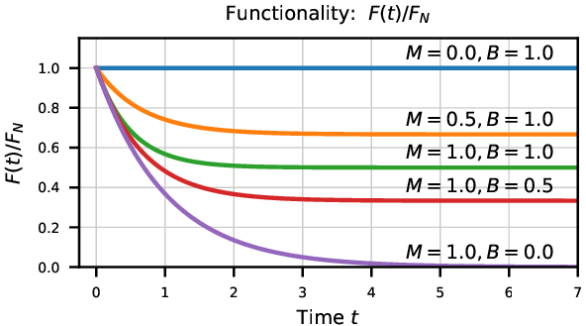
Figure 2: Normalized functionality, ${{F}}(t)/F_{\text{N}}{}$, is shown for various values of $\mathcal{M}$ (malware attacking) and $\mathcal{B}$ (bonware defending) and initial condition ${{F}}(0)=F_{\text{N}}{}$. The functionality over time depends on the relative strengths of bonware and malware. With the system initially at normal functionality and malware effectiveness nonzero, functionality exhibits exponential decay.

If ${{F}}(0)>\nicefrac{{F_{\text{N}}{}\mathcal{B}}}{{\mathcal{Q}}},$ then ${{F}}(t)$, initially at ${{F}}(0)$ at time $t\leavevmode\nobreak\ =\leavevmode\nobreak\ 0$, will decrease to $\nicefrac{{F_{\text{N}}{}\mathcal{B}}}{{\mathcal{Q}}}$ (see Figure 2). If ${{F}}(0)\leavevmode\nobreak\ >\leavevmode\nobreak\ \nicefrac{{F_{\text{N}}{}\mathcal{B}}}{{\mathcal{Q}}},$ then the function ${{F}}(t)={{F}}(0)$ will be constant. If ${{F}}(0)<\nicefrac{{F_{\text{N}}{}\mathcal{B}}}{{\mathcal{Q}}},$ the function will start at ${{F}}={{F}}(0)$ and increase to $\nicefrac{{F_{\text{N}}{}\mathcal{B}}}{{\mathcal{Q}}}.$ The plots for $\mathcal{M}>0$ in Figure 2 show that even in the presence of bonware, malware has an impact on the system. The steady-state of the system is obtained either by setting $\frac{d{{F}}}{dt}=0$ in Equation 6 or letting $t\to\infty:$

$${{F}}_{\infty}=\lim_{t\to\infty}{{F}}(t)=F_{\text{N}}{}\frac{\mathcal{B}}{\mathcal{M}+\mathcal{B}}$$ (8)

so that the antidote to malware is to overwhelm it with bonware. The exponent, $-\mathcal{Q}t=(-\mathcal{M}-\mathcal{B})t$ in the solution given by Equation 7 indicates that increasing the effectiveness of either malware or bonware will cause the system to more quickly approach steady-state. At steady-state,

$$\frac{F_{\text{N}}{}-{{F}}_{\infty}}{{{F}}_{\infty}}=\frac{\mathcal{M}}{\mathcal{M}+\mathcal{B}}.$$ (9)

Equation 9 gives us further insight into the trade-off between effectivenesses of both malware and bonware. The relative decrease of the function from normal functionality is equal to the ratio of malware effectiveness to the sum of malware and bonware effectivenesses.

IV-C Piecewise constant model

If either malware’s or bonware’s effectiveness diminishes at some point in the incident, the model may switch from one set of constants defining malware and bonware to another set of constants. The differential equation (Eq. 5) may now be expressed as

$$\frac{d{{F}}}{dt}=\sum_{j=0}^{N-1}(F_{\text{N}}{}-{{F}}(t))\mathcal{B}_{j}(t)-{{F}}(t)\mathcal{M}_{j}(t),$$ (10)

where the vectors $\boldsymbol{\mathcal{M}}=({\mathcal{M}}_{0},{\mathcal{M}}_{1},\cdots{\mathcal{M}}_{N-1})$ and $\boldsymbol{\mathcal{B}}=({\mathcal{B}}_{0},{\mathcal{B}}_{1},\cdots,{\mathcal{B}}_{N-1})$ contain the malware effectivenesses and bonware effectivenesses within time windows whose end points are defined by $\{t_{0},t_{1},\cdots,t_{N}\}$. The solution will be a function which, in each time interval, is the solution found in Equation 7:

$${{F}}(t)=\left[{{F}}(t_{j})-\frac{F_{\text{N}}{}\mathcal{B}_{j}}{\mathcal{Q}_{j}}\right]e^{-\mathcal{Q}_{j}\cdot(t-t_{j})}+\frac{F_{\text{N}}{}\mathcal{B}_{j}}{\mathcal{Q}_{j}},$$

$$\quad(t_{j}\leq t<t_{j+1}),\quad(j=0,\cdots,N-1)$$

where $\mathcal{Q}_{j}=\mathcal{M}_{j}+\mathcal{B}_{j}$. The purple curve in Figure 3 is an example realization of this model.

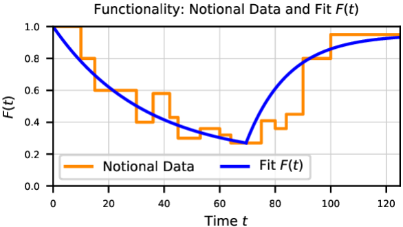
Figure 3: The smooth curve is an example functionality curve with piecewise constant malware and bonware effectivenesses. The notional data and piecewise constant model fit are described in Section IV-F.

IV-D Linear model

The effectivenesses of malware and bonware may also be linear functions of $t$, so that $\mathcal{M}(t)=\nu-\mu t$, $\mathcal{B}(t)\leavevmode\nobreak\ =\leavevmode\nobreak\ \alpha\leavevmode\nobreak\ -\leavevmode\nobreak\ \beta\leavevmode\nobreak\ t$, and $\mathcal{Q}(t)=\lambda-\omega t$, where $\lambda=\alpha+\nu$ and $\omega=\beta+\mu$. Under this linear model, Equation 5 becomes

$$\frac{d{{F}}}{dt}+(\lambda-\omega t){{F}}(t)=F_{\text{N}}{}(\alpha-\beta t).$$ (11)

The solution can be expressed in terms of the error function $\operatorname{erf}(z)=\frac{2}{\sqrt{\pi}}\int_{0}^{z}e^{-\tau^{2}}\,d\tau$:

$$\frac{{{F}}(t)}{F_{\text{N}}{}} =\frac{1}{\Omega(t)}\left\{\frac{{{F}}(0)}{F_{\text{N}}{}}-\frac{\beta}{\omega}\left(1-{\Omega(t)}\right)+(\alpha\omega-\beta\lambda)\right.$$ (12)

$$\times \left.\frac{\sqrt{\frac{\pi}{2}}e^{\Lambda^{2}}}{\omega^{3/2}}\left[\operatorname{erf}\left(\Lambda\right)+\operatorname{erf}\left(\frac{\omega t}{\sqrt{2\omega}}-\Lambda\right)\right]\right\}$$

where $\Omega(t)=e^{\lambda t-\frac{1}{2}\omega t^{2}}$, and $\Lambda=\nicefrac{{\lambda}}{{\sqrt{2\omega}}}$.

IV-E Piecewise linear model

Both malware and bonware effectivenesses may initially be linear, but if the situation changes and a different linear model holds after a time, the model should be able to account for it. In particular, if malware effectiveness is decreasing over time, at some point we will reach $\mathcal{M}=0$ and the model switches to a new linear model. Equation 11 can be written

$$\frac{d{{F}}}{dt}=\sum_{j=0}^{N-1}\left[(\lambda_{j}-\omega_{j}t){{F}}(t)-F_{\text{N}}{}(\alpha_{j}-\beta_{j}t)\right].$$

The solution follows from Equation 12:

$$\frac{{{F}}(t)}{F_{\text{N}}{}} =\frac{1}{\Omega_{j}(t)}\left\{\frac{{{F}}(t_{j})}{F_{\text{N}}{}}-\frac{\beta_{j}}{\omega_{j}}\left(1-\Omega_{j}(t)\right)+(\alpha_{j}\omega_{j}-\beta_{j}\lambda_{j})\right.$$

$$\times \left.\frac{\sqrt{\frac{\pi}{2}}e^{\Lambda_{j}^{2}}}{\omega_{j}^{3/2}}\left[\text{erf}\left(\Lambda_{j}\right)+\text{erf}\left(\frac{\omega_{j}(t-t_{j})}{\sqrt{2\omega_{j}}}-\Lambda_{j}\right)\right]\right\},$$

$$\quad(t_{j}\leq t<t_{j+1}),\quad(j=0,\cdots,N-1)$$

where $\Omega_{j}(t)=e^{\lambda_{j}(t-t_{j})-\frac{1}{2}\omega_{j}(t-t_{j})^{2}}$ and $\Lambda_{j}=\nicefrac{{\lambda_{j}}}{{\sqrt{2\omega_{j}}}}$.

Example realizations of the piecewise linear models are shown in Figure 4.

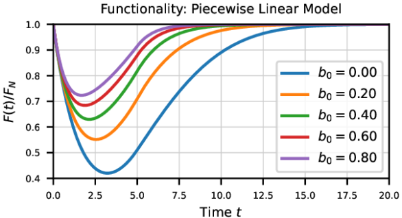
Figure 4: Normalized functionality, ${{F}}(t)/F_{\text{N}}{}$, is shown for piecewise linear models and initial condition $F(0)=F_{\text{N}}{}$. Both malware and bonware effectivenesses are initially linear functions of time: $\mathcal{M}\leavevmode\nobreak\ =\leavevmode\nobreak\ \max(0.5-0.1t,0),\mathcal{B}=b_{0}+0.04t.$ When malware effectiveness reaches $\mathcal{M}=0$, bonware effectiveness continues to increase.

IV-F Obtaining model parameters

Given data that represents functionality over the course of an incident where malware and bonware are active, we develop a fast method to estimate the continuous model parameters for a curve that approximates the data, and use these parameters to generate further realizations based on this model. In Figure 3, notional data is shown (in orange) and the parameters $\mathcal{M}$ and $\mathcal{B}$ are estimated and a fit for the functionality $F(t)$ is found that solves the piecewise constant model expressed by Equation 10. In this section, we illustrate our fast method to extract the model parameters from this curve.

The set $P=\{t_{0},\ldots,t_{K}\}$ partitions the scenario timeline, and malware and bonware are constant in each interval $(t_{i-1},t_{i}),\,\,i=1,\ldots,K.\,\,$ In each interval, $\mathcal{Q}_{i}=\mathcal{M}_{i}+\mathcal{B}_{i}$ and the differential equation governing Continuous Model I is $\frac{dF(t)}{dt}+\mathcal{Q}_{i}F(t)=F_{\text{N}}{}(t)\mathcal{B}_{i}.$ Thus, in each interval $(t_{i-1},t_{i}),$ the solution is

$${{F}}(t)=\left[{{F}}(t_{i-1})-\frac{F_{\text{N}}{}\mathcal{B}_{i}}{\mathcal{Q}_{i}}\right]e^{-\mathcal{Q}_{i}(t-t_{i-1})}+\frac{F_{\text{N}}{}\mathcal{B}_{i}}{\mathcal{Q}_{i}}.$$

We compute the effectiveness of malware $\mathcal{M}_{i}$ and the effectiveness of bonware $\mathcal{B}_{i}$ in each interval.

We observe that there is a unique switching time $t^{\star}$ where the functionality’s trend reverses, and thus we take $K=2.$ Before the switch, the effectiveness of malware is greater than that of bonware. From the time of the switch until the end of the run, bonware is stronger. To estimate the switching time $t^{\star}$, we find the minimum of the data to occur over the interval from 64 s to 75 s. There, the minimum value of the data curve is $m=0.27$. Taking the midpoint, our estimate for $t^{\star}$ is 69.5 s.

We numerically solve this system of equations:

$$\alpha m =F_{\text{N}}{}\frac{\mathcal{B}_{1}}{\mathcal{Q}_{1}},$$

$$m ={{F}}(0)-F_{\text{N}}{}\frac{\mathcal{B}_{1}}{\mathcal{Q}_{1}}e^{-\mathcal{Q}_{1}t^{\star}}+F_{\text{N}}{}\frac{\mathcal{B}_{1}}{\mathcal{Q}_{1}}.$$

The first equation says that where the curve meets the minimum of the data, it has experienced exponential decay of $\alpha$ toward the asymptotic minimum. We take $\alpha$ to be $\alpha=1-\nicefrac{{1}}{{e}}$. The second equation says that the minimum occurs at the switching time (the time when the model switches from malware dominating bonware, to bonware dominating malware). Solving this system of equations yields (with $\mathcal{M}_{1}=\mathcal{Q}_{1}-\mathcal{B}_{1}$), $\mathcal{M}_{1}\approx 0.025$ and $\mathcal{B}_{1}\approx 0.005$. To the right of $t^{\star}$, we fit an exponentially increasing function by numerically solving this system of equations:

$$\zeta =\frac{F(0)\mathcal{B}_{2}}{\mathcal{Q}_{2}},$$

$$\tilde{\alpha}\zeta =\left(m-\frac{F_{\text{N}}{}\mathcal{B}_{2}}{\mathcal{Q}_{2}}\right)\!\!\left(e^{-\mathcal{Q}_{2}(125-t^{\star})}+\frac{F_{\text{N}}{}\mathcal{B}_{2}}{\mathcal{Q}_{2}}\right).$$

We have found that $\tilde{\alpha}=1-e^{-4}$ and $\zeta=0.95$ are satisfactory values to use for these hyperparameters. We compute $\mathcal{M}_{2}\approx 0.005$ and $\mathcal{B}_{2}\approx 0.088$.

V Experimental Testbed and Method

A key role of the mathematical models presented above is to help analyze results of actual experimental measurements of resilience. In this section, we introduce the experimental test bed and experimental process we use to observe and characterize cyber resilience of a truck [26]. In a typical resilience-measuring experiment, the following occurs, conceptually: (1) The truck is assigned a goal (delivering a cargo to a destination, along a specified route). The truck begins to accomplish the goal. The driver controls the truck aiming to maximize probability of the goal’s success. (2) At some point along the route, an adversarial cyber effect is activated and begins to degrade goal-relevant performance of the truck. (3) Physical and cyber elements within the truck begin to resist the impact of the cyber effect. After some time, these elements (i.e., bonware, collectively) may succeed in recovering some or all of the degraded performance. (4) The data collection and logging system obtains and records the performance parameters of the truck over time, from the beginning of the run until its end (successful or otherwise). The data are later analyzed using the models presented earlier.

These processes and functions are implemented in several components of the test bed, which include automotive hardware and simulation software: the Toyota Portable Automotive Security Testbed with Adaptability (PASTA) by Toyota Motor Corporation, the Unity game development platform, Active Defense Framework (ADF) developed at the DEVCOM Army Research Laboratory, and the OpenTAP test automation framework by Keysight Technologies. These components and their roles are described in subsections below. In terms of interactions between the components, Unity generates messages via the Message Queue Telemetry Transport (MQTT) publish-subscribe network protocol. ADF ingests these messages and translates them to Controller Area Network (CAN) format, which are then injected onto the appropriate CAN bus within PASTA. Figure 5 illustrates the flow of data between components.

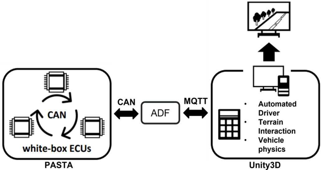
Figure 5: A high-level overview of the data flow between components. Portions are derived from [27].

V-A PASTA

PASTA is a cyber-physical product by Toyota, intended to develop and evaluate new vehicle security technology and approaches on realistic “white-box” electronic control units [27]. There are three vehicle ECUs provided within the product, each with its own CAN bus: powertrain, body, and chassis. These three ECUs are responsible for their respective group of messages, each generating and responding to traffic on their bus. A fourth ECU, the central gateway (CGW), acts as a junction between the three previously mentioned buses. Based on the message and source bus, the CGW ferries messages to their appropriate destination bus. The firmware for all ECUs is open-source, and is accompanied by an integrated development environment (IDE).

PASTA includes simulation boards which calculate how the current CAN messages on the buses would physically influence a commercial sedan. These boards then update the vehicle ECUs with appropriate values. For example, when acceleration pedal operation is inputted, the chassis ECU sends a message with the indicated value. The simulation boards observe this message and calculate the physical effects that would result from the input. The results are used to update the values reported by the powertrain ECU, which it outputs onto its bus. In this instance, the powertrain ECU would send messages indicating the new engine throttle position, revolutions per minute (RPM), and speed. Unfortunately, we found the simulation boards rather constraining, for our purposes. We cannot alter, for instance, the parameters involving the engine (e.g., torque and horsepower), the weight of the vehicle, or the terrain that the boards are assuming is being traversed. To overcome these constraints, we integrated a simulation engine (Unity, see below) that would allow for user-defined vehicle details as well as custom terrain. In this configuration, PASTA becomes hardware-in-the-loop for the simulation engine. Cyber attacks or defenses that affect the ECUs present in PASTA will also affect the performance of the truck within the simulation.

V-B Unity

Unity is a widely used game development platform [28]. In particular, Unity provides built-in assets and classes regarding vehicle physics, which we leverage to model interactions between our simulated truck and custom terrain.

V-B1 Simulated Trucks

We implemented three types of truck within Unity – light, medium, and heavy. They are designed to interface with data inputs from the white-box ECUs within PASTA. In an experiment, the current chosen truck produces inputs in response to the simulated terrain. These inputs are sent to the corresponding ECUs within PASTA. We then gather responses to these inputs from the ECUs and send them back to the truck, which it uses to calculate parameters like torque and fuel consumption. For example, assume the truck reports that the accelerator is set to 50%. This message is injected into PASTA as if the chassis ECU had generated it. The powertrain ECU responds to the message with the corresponding amount of engine throttle. A message with the engine throttle is sent back to Unity, which is then applied to engine power calculations. With this flow, any cyber attacks impacting the ECUs within PASTA will affect the truck.

An automated driver is responsible for generating steering, acceleration, and braking inputs as the truck traverses the terrain. Steering is guided using a waypoint system. Both acceleration and braking inputs are calculated via a proportional-integral-derivative (PID) controller guided by a target speed. The controller responds to changes in the terrain or truck performance, and maintains the target speed while preventing oscillation. Optional target speed variability simulates driver attention drift, which may be used to generate multiple unique realizations of the simulation under otherwise identical conditions.

Engine performance is calculated through the use of torque, horsepower, and brake-specific fuel consumption (BSFC) curves. Engine RPM is derived using the speed, wheel circumference, and effective gear ratio. Using this RPM value, the curves are evaluated to discern the corresponding torque, horsepower, and BSFC value. Torque is multiplied by the throttle and the current effective gear ratio to obtain the total amount of torque that can be applied to the wheels. Since our trucks are all-wheel drive (AWD), each wheel receives the total amount of torque divided by the number of wheels on the truck. Horsepower and the BSFC value are used in conjunction to calculate the amount of fuel that has been used per physics update.

The truck is capable of providing sensor information that is either not present in PASTA or needs its functionality altered for our purposes. Currently, this applies to the engine coolant temperature, attitude sensor, and a set of backup engine ECUs. Engine temperature is present in PASTA, but is aligned to the temperature characteristics of a static commercial sedan. Within Unity, we implemented a temperature model that can be controlled by an external fan controller ECU. The fan controller monitors the coolant temperature reported by the truck and dictates the operation of a simulated fan on the truck. The fan itself takes significant power to operate, which results in a drop in the available torque that can be applied to the wheels.

V-B2 Terrain

The truck within Unity traverses a custom terrain map that is roughly 81.8 km by 100 km with altitudes up to 910 m. We crafted a course approximately 151 km in length across the map that encompasses multiple terrain types: flat main road, flat off-road, hilly, prolonged ascent, and prolonged descent. On a flat main road, the target speed is 60 km per hour. Otherwise, the target speed is 40 km per hour.

V-C Active Defense Framework

ADF is a government-developed framework for prototyping active cyber-defense techniques. ADF currently supports Internet Protocol (IP) networks and vehicle control networks, namely the CAN bus and Society of Automotive Engineers (SAE) J1708 bus. The framework acts as an intermediary for network traffic, as depicted in Figure 5, allowing it to control network message flow, as well as inspect, modify, drop, or generate network messages. In our experimental test bed, ADF enables communication between PASTA and Unity by translating CAN messages to and from MQTT, a standard publish-subscribe IP-based messaging protocol. ADF plugins are also used to provide simulated ECU hardware, and to implement cyber attack and defense methods on the CAN bus via ADF’s ability to monitor, modify, inject, or drop CAN traffic.

V-C1 Unity-to-PASTA Message Translation

ADF and Unity run on a standalone laptop and are connected to PASTA via two universal serial bus (USB) CAN over Serial (SLCAN) interface modules. One module is connected to the powertrain CAN bus, and the other module is connected to the chassis CAN bus. The PASTA CGW is disconnected from the CAN buses for our experiments, and the body CAN bus and body ECU are not used. ADF is configured to serve as a CGW between Unity and PASTA. Since Unity does not natively communicate with CAN interfaces, ADF translates CAN messages in real-time to MQTT messages and back. Unlike the PASTA CGW, ADF does not relay messages between the powertrain and chassis CAN buses themselves. ADF relays powertrain CAN messages between Unity and PASTA, and sends parameters from Unity to the chassis CAN bus for display on the PASTA instrument cluster. All communication channels are two-way.

V-C2 Virtual ECUs within ADF

For some cyber attacks, a virtual ECU is needed. For example, as mentioned before, the PASTA platform does not simulate a controllable cooling fan or provide fan controller ECU functionality. Therefore, we simulate a fan controller ECU using an ADF plugin. The fan controller engages the engine cooling fan on the truck when the engine coolant temperature reaches a defined upper limit, and disengages the fan when temperature drops below a lower limit. For the purposes of our experiments, the fan controller ECU plugin can simulate an attack on its own firmware, stop the attack, or reset/“re-flash” itself (i.e., replace the ECU firmware). During a reset, the fan controller is offline for a period of time. Use of ADF enables creation of other simulated ECUs and corresponding cyber attacks.

V-C3 Performing Cyber Attacks via ADF

A class of attacks on a vehicle bus involves injecting messages. Messages are broadcast on a CAN bus, so one message injected at any point on the bus will reach all ECUs on the bus. While injection attacks cannot block or modify normal CAN bus traffic, they can impact vehicle performance if injected messages cause undesired vehicle behavior. If an attacker can physically sever the CAN bus wiring at a strategic point and place additional hardware there, it is possible to block or modify the normal bus traffic. Cyber attacks that block or modify messages can prevent ECUs from controlling the vehicle or falsify vehicle data.

As a man-in-the-middle between PASTA and Unity, ADF can execute any of these bus-level attack types.

Cyber attacks on ECU firmware, by embedding malware, are also feasible. We have simulated the effects of embedded malware in three instances: on the fan controller, the suspension controller, and the main engine ECU. Malware on the fan controller simulates a “stuck fan” attack in which malware has modified the fan control ECU to not disengage the fan once engaged, even when the coolant temperature has dropped below the minimum operational temperature; the suspension controller attack creates the appareance that the truck is abnormally tilted, forcing the truck into a safe “limp home” mode that reduces the amount of available gears; the main engine ECU attack causes erratic performance behavior.

V-C4 Performing Cyber Defensive Actions via ADF

Defending against message injection, blocking, and modification at the bus-level requires detecting and filtering injected messages before they reach the ECU. The CAN bus can be split at potential access points and hardware placed in-line, hardware can be placed between the CAN bus and critical ECUs, or defenses can be integrated into the ECUs themselves. Examples of these defenses implemented previously using ADF include cryptographic watermarking and modeling observable vehicle states to compare current parameters to the model’s prediction.

Cyber attacks on ECUs themselves must be approached differently. If an ECU is compromised, measures need be taken to restore proper ECU function. Many ECUs can be re-flashed while the vehicle is operational. The ECU may or may not be functional for some duration while being reset or re-flashed, and the impact this will have on vehicle performance depends on the function of the ECU. For the ECUs simulated by ADF plugins, the behavior is to make the ECU unresponsive for a set duration, after which normal ECU operation is restored. Note, for ECUs like the main engine ECU, this is not possible because the vehicle will become inoperable in its absence. To address this, a manually-crafted ECU backup is used while the main ECU is re-flashed.

V-D OpenTAP and Data Collection

OpenTAP is an open-source test automation framework developed by Keysight Technologies [29]. It provides a test sequencer to promote test repeatability, a customizable plugin facility capable of integrating plugin classes implemented in C# or Python, and result listeners responsible for capturing test data for further analysis. OpenTAP is used to automate the execution of experiments and provide a GUI for testing practitioners to configure experiment steps.

Data are captured from the truck. Examples of data are fuel efficiency, speed, engine torque, and acceleration pedal input; each data value comes with a timestamp of the value occurrence.

V-E Execution of Experiments

Each individual experimental run follows the same set of steps. During setup, we establish CAN connections to PASTA, ensure the messaging infrastructure is running, and start Unity. During parameter selection, we determine the truck type, cargo weight, type of cyber attack, etc., and designate the number of runs. During execution, we run automated test scripts with the given parameters and capture the data in a desired format. Finally, we parse and preprocess the data, fit our mathematical models, and generate graphs and results.

An experiment reflects execution of a single run as described in the beginning of this section. On our terrain, a typical run would take 2-3 hours to traverse in its entirety. However, we focus on shorter 15-minute runs that encompass a cyber attack at variable moments within the run and a potential recovery. Note that it may take the truck several minutes to recover from the attack. We are also capable of executing faster-than-real-time when using solely simulated components, further decreasing execution time of experiment runs.

To form a series of experiments, within our test bed, there are multiple parameters that can be configured to generate varied data captures. Currently, these include: truck type, experiment duration, cyber attack start time, terrain type(s), starting location, ending location, target speed, cyber attack-defense pairings, cargo weight, and target speed variability.

VI Experimental Data

Using our test bed, we conducted a series of experimental runs in which a truck is subjected to a cyber attack. Here we focus on one of these series. In this series of experiments, we considered three types of trucks with four possible cargo weights including $0$, the five unique terrains described above, and three types of cyber attacks, including one “baseline” scenario with no cyber attack (see Table I). For each combination of these, we conducted 30 experimental runs and recorded the truck’s speed, fuel efficiency, and other operating parameters. The 30 runs were made unique by adding random variability to the driver’s interaction with the accelerator (i.e., “driver attention drift” as described in Subsection V-B).

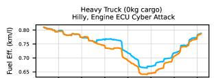
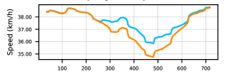
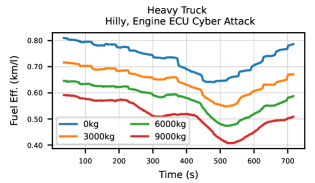
Figure 6: Examples of experimental data, illustrating that cyber attacks reduce performance both in fuel efficiency (top panel) and speed (middle panel), and that changes in cargo weight reduce fuel efficiency in the expected manner (bottom panel). Top panel: The fuel efficiency of a heavy truck, carrying no cargo, during a run on hilly terrain. The orange curve indicates the fuel efficiency in the “engine ECU attack” run, which is contrasted with the (partly occluded) cyan curve that indicates the baseline run. Middle panel: Recorded speed during the same run. Bottom panel: Fuel efficiency, now for all four cargo conditions (from top to bottom: 0, 3,000, 6,000, and 9,000kg).

Table I: Overview of Experimental Design

Independent variable	Possible values
3 trucks	{ Light, Medium, Heavy }
5 terrains	{ Steady Descent, Flat Road, Flat Off-Road, Hilly, Steady Ascent }
4 cyber attack scenarios	{ Baseline, Fan, ECU, Suspension }
4 cargo weights	{ None, Light, Medium, Heavy }
30 random seeds	{1 …30}

VI-A Data Preprocessing

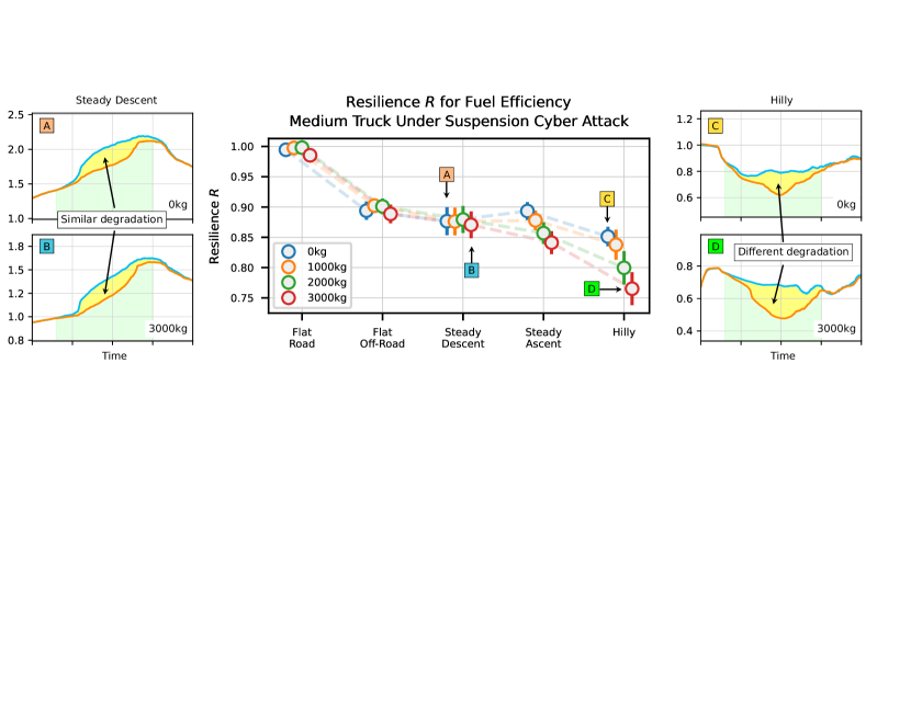
Figure 7: An illustration of the resilience measure $R$. The central panel shows the value of $R$ for 20 different conditions (five subroutes and four cargo weights). Each marker shows $R$ computed using the average of 30 runs of a suspension cyber attack and the average of 30 baseline runs (error bars indicating 95% confidence intervals), in this case by a medium-weight truck. The panel thus summarizes 1,200 experimental runs. The four side panels illustrate the construction of $R$. Each side panel shows the construction of one marker in the central panel. The blue (upper) curve indicates functionality under the baseline scenario. Note that the baseline functionality differs between subroutes (left vs. right panels) and between cargo weight conditions (top vs. bottom). The orange (bottom) curve indicates the functionality during the cyber attack. The shaded yellow region between the curves is the effect of the attack: a temporary reduction in functionality. $R$ is the ratio of area under the orange curve to that under the blue curve (Eq. 2) and can be interpreted as a measure of resilience: it is the remaining fraction of functionality while under attack. Those values of $R$ are displayed in the central panel, which shows that resilience is high on flat road, but lower on hilly terrain. It further shows a notable effect of cargo weight in the hilly terrain as well as during the steady ascent, but no effect of cargo weight in the steady descent, flat road, or flat off-road subroutes.

The operating parameters were recorded at a relatively high frequency of about 50 Hz, which sometimes causes numerical instability (e.g., in calculating fuel efficiency over a 20 ms period). For this reason, we first applied a smoothing filter to the data. We chose a running median filter with a window of 72 s. The running median has the advantage that it downweights extreme values that might result from numerical inaccuracy. We then took the mean of the 30 runs in each condition to obtain the relatively smooth time series seen in Figure 6.

The three panels of Figure 6 each show the time course of a performance parameter. The top two panels each show one curve for the baseline run (cyan) and one for an attack run (orange). The bottom panel shows four attack runs with different cargo weights.

VI-B Resilience $R$

We will use the experimental data to compute the $R$ statistic introduced in Equation 2 in subsection III-B. The computation of $R$ is illustrated in Figure 7. The calculation involves (1) finding the area $\mathcal{A}_{\text{attack}}$ under the performance curve during the time when the cyber attack is active, then (2) finding the corresponding area $\mathcal{A}_{\text{baseline}}$ under the baseline performance curve, and (3) dividing the former by the latter. If the resulting $R$ is $1.0$, then the cyber attack had no detrimental effect on performance. $R$ of $0.0$ means that performance was reduced by 100%.

VI-C Modeling Approach

Our modeling approach requires one further data processing step, which is illustrated in Figure 8. The top panel shows a baseline and attack performance curve. The ratio of these curves (i.e., performance under attack divided by the baseline value) is shown in the middle panel – this ratio is close to $1.0$ when performance under cyber attack is similar to the baseline performance, and less than $1.0$ when the cyber attack is detrimental to performance. This performance ratio is the measure of functionality that we use for our modeling. In the bottom panel, we show the fitted “piecewise constant” model that is described in Subsection IV-C. The red and green intervals indicate the activity periods of the malware and bonware, respectively. When they are inactive, these effectiveness parameters are $0$, otherwise they are $M$ and $B$ respectively. We can see that the model captures the drop in performance when the malware is active.

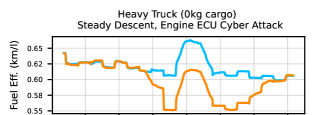
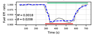
Figure 8: Progression of data over time. Top panel: Fuel efficiency of a heavy truck, carrying no cargo, during a run on steadily descending terrain (orange: Engine ECU attack run; cyan: baseline run). Bottom panel: The fuel efficiency ratio (solid grey line) is the performance in the attack run divided by the performance in the baseline run. The overlaid, blue dashed line, is the fit of the continuous model. The green and red horizontal lines at the top and bottom indicate the times when the bonware and malware (resp.) are active. The model captures the rapid decline to an equilibrium state around 92% performance as well as the more gradual recovery after the cyber attack.

To summarize and interpret our data, we applied this model to the data from each experimental condition separately. In order to automate the parameter estimation process, we implemented our piecewise constant model using a Bayesian inference engine [30, 31]. To further facilitate the automation, we additionally allowed the model to estimate the time points where performance begins to decline ($t_{1}$) and recover ($t_{2}$). This implementation is considerably slower than the fast method developed above in subsection IV-F, but it has the advantage of being fully automatic and easily extendable for future projects. The method has the additional advantage that it lets us quantify the uncertainty in parameter estimates.

VII Discussion of Results

VII-A Experimental Results

Considering the large scope of our experiment, we focus on examples of the types of conclusions we are able to draw.

First, as Figures 6, 7, and 8 show, our cyber attacks cause decreases in performance in the expected parameters at the expected times. For example, the cyber attack on the suspension causes a reduction in fuel efficiency and speed compared to the baseline scenario. We also see a slight square-wave pattern with a period of 72 s, corresponding to the normal behavior of the engine cooling fan periodically engaging and disengaging. We also see that fuel efficiency decreases as cargo weight increases.

VII-B Resilience $R$

Figure 7 illustrates that the resilience measure $R$ (based on the area under the curve concept) follows our intuitive understanding of what a measure of cyber resilience should do: it is higher if performance is impacted by cyber attack less, and lower if it is impacted more. It is relatively unimpacted in cases where no impact was expected (e.g., on the flat road subroutes in Fig. 7, there is no difference between cargo weight conditions), and it gives orderly results when differences are expected (e.g., when in Fig. 7 the $R$ is affected by cargo weights, it is consistently lower for heavier cargo).

The top panel of Figure 9 shows results for the same truck when it is subjected to the cyber attack on the engine fan controller. Here, we see a different pattern of results, with the effect generally being greater when the cargo is lighter. However, the results remain ordered and show a great deal of consistency. There seems to be much less difference between subroutes during this attack. Also, on average, the loss of functionality due to this attack is smaller than that due to the attack on the engine ECU.

Taken together, our experimental data support the validity of the $R$ measure as a quantitative measure of cyber resilience.

VII-C Modeling Results

As illustrated in Figure 8, our mathematical model and the experimental data exhibit a similar pattern and the model produces a good fit. Moreover, the estimates of parameters $M$ and $B$ attain values that reflect the temporal behaviors of experimental data (e.g., high $B$ is associated with rapid recovery, and the ratio of $B/(M+B)$ approximates the performance equilibrium when the cyber attack is active).

The modeling approach allows us to summarize complex time series with two interpretable parameters: the malware effectiveness $M$ and the bonware effectiveness $B$. This facilitates comparison of the cyber resilience of our trucks under various conditions. For example, Figure 9 shows the pattern of results of an engine ECU cyber attack on a heavy truck (note: higher $B$ means more effective bonware and higher $M$ means more effective malware). At a glance at the middle panel, we can determine that the truck resists the cyber attack better when it is not hauling cargo (blue markers are always higher), and especially so when the terrain is a steady ascent (the difference is especially pronounced in that subroute). The bottom panel shows that the cyber attack is relatively more effective when the cargo is light (blue markers are often higher) and especially the road is flat (the blue line has its peak there). Comparing the magnitude of the parameter estimates between the two panels ($B$ is greater than $M$ by at least an order of magnitude) tells us that this cyber attack, even at its most effective, only has a modest effect on functionality.

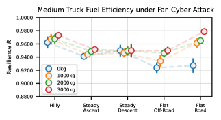
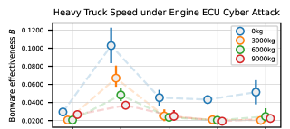
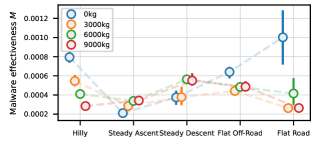
Figure 9: Example results of experiments. Round markers indicate parameter estimates, the intervals around the markers are 95% credible intervals. Each panel summarizes 1,200 runs (5 terrains by 4 cargo weights by 30 repetitions, once under baseline and once under cyber attack). Top: The $R$ measure for a medium truck subjected to a fan cyber attack. Middle and bottom: Parameter estimates of the piecewise continuous model applied to performance of a heavy truck under a cyber attack on the engine ECU. The middle panel displays the effectiveness of the bonware as a function of terrain and cargo weight, while the bottom panel displays effectiveness of the malware. One observation is that the effectiveness of the bonware is generally much higher than that of the malware, largely due to the physical resilience of the truck machinery.

VIII Conclusions and Future Work

We have reported results of the Quantitative Measurement of Cyber Resilience project, in which we obtain experimental data with physical-digital twins of several cargo trucks and analyze the data with mathematical modeling of time series in order to quantify and measure the cyber resilience of the trucks. We were successful in generating data with apparent fidelity, showing that changes in the setup of the experimental runs (e.g., heavier cargo, more challenging terrain) result in differences in performance that accord with our subject matter expertise as well as common sense expectations.

We proposed two types of summary statistics. One is a measure of resilience based on the area under the performance curve. Another type is based on fits of a mathematical model to temporal evolution of the performance curve, and measures the effectiveness of malware and bonware. These measures seem to capture the salient patterns in the experimental data succinctly, supporting their use as quantitative measures of cyber resilience.

We believe there is much that could still be learned with our (or a similar) test bed. Data is relatively easy and fast to gather, and more variables can still be introduced. Additionally, similar test beds could be constructed for other types of vehicles, but also for other diverse types of complex equipment, infrastructure, or critical digital services. For the trucks, the test bed could still be augmented with additional derived measures of functionality, such as maneuverability.

Similarly, there are further potential developments in the mathematical modeling aspect. New models could be implemented to allow for multivariate functionality, to account for trade-offs between different performance parameters.

References

- [1] A. Kott, M. Weisman, and J. Vandekerckhove, “Mathematical modeling of cyber resilience,” Proceedings of IEEE Military Communications Conference, pp. 835–840, Dec. 2022.
- [2] M. Weisman, A. Kott, and J. Vandekerckhove, “Piecewise linear and stochastic models for the analysis of cyber resilience,” 57th Annual Conference on Information Sciences and Systems, Mar. 2023.
- [3] A. Kott and I. Linkov, Cyber resilience of systems and networks. New York, NY: Springer International Publishing, 2019.
- [4] S. C. Smith, “Towards a scientific definition of cyber resilience,” in 18th International Conference on Cyber Warfare and Security (ICCWS 2023). Red Hook, NY: Academic Conferences Ltd, Mar.9–10 2023, pp. 1–9.
- [5] I. Linkov, B. D. Trump, and J. Keisler, “Risk and resilience must be independently managed,” Nature, vol. 555, p. 7694, 2018.
- [6] M. Bozdal, M. Samie, and I. Jennions, “A survey on CAN bus protocol: Attacks, challenges, and potential solutions.” in 2018 International Conference on Computing, Electronics & Communications Engineering. Ieee, August 2018, pp. 201–205.
- [7] A. Kott, P. Théron, M. Drašar, E. Dushku, B. LeBlanc, P. Losiewicz, …, and K. Rzadca, “Autonomous intelligent cyber-defense agent (aica) reference architecture,” 2018, arXiv:1803.10664.
- [8] A. Kott, M. S. Golan, B. D. Trump, and I. Linkov, “Cyber resilience: by design or by intervention?” Computer, vol. 54, no. 8, pp. 112–117, 2021.
- [9] A. Kott and P. Theron, “Doers, not watchers: Intelligent autonomous agents are a path to cyber resilience,” IEEE Security & Privacy, vol. 18, no. 3, pp. 62–66, 2020.
- [10] A. Alexeev, D. S. Henshel, K. Levitt, P. McDaniel, B. Rivera, S. Templeton, and M. Weisman, “Constructing a science of cyber-resilience for military systems,” in NATO IST-153 Workshop on Cyber Resilience, 2017, pp. 23–25.
- [11] D. S. Henshel, K. Levitt, S. Templeton, M. G. Cains, A. Alexeev, B. Blakely, P. McDaniel, G. Wehner, J. Rowell, and M. Weisman, “The science of cyber resilience: Characteristics and initial system taxonomy,” Fifth World Conference on Risk, 2019.
- [12] A. K. Ligo, A. Kott, and I. Linkov, “How to measure cyber-resilience of a system with autonomous agents: Approaches and challenges,” IEEE Engineering Management Review, vol. 49, no. 2, pp. 89–97, 2021.
- [13] I. Linkov, D. A. Eisenberg, K. Plourde, T. P. Seager, J. Allen, and A. Kott, “Resilience metrics for cyber systems,” Environment Systems and Decisions, vol. 33, no. 4, pp. 471–476, 2013.
- [14] P. Beling, B. Horowitz, and T. McDermott, “Developmental test and evaluation (DTE&A) and cyberattack resilient systems,” Systems Engineering Research Center, Hoboken, NJ, Technical Report Serc-2021-tr-015, September 2021.
- [15] S. Hosseini, K. Barker, and J. E. Ramirez-Marquez, “A review of definitions and measures of system resilience,” Reliability Engineering & System Safety, vol. 145, pp. 47–61, 2016.
- [16] A. Kott and I. Linkov, “To improve cyber resilience, measure it,” Computer, vol. 54, no. 2, pp. 80–85, Feb. 2021.
- [17] T. Hoppe and J. Dittman, “Sniffing/replay attacks on can buses: A simulated attack on the electric window lift classified using an adapted cert taxonomy,” in Proceedings of the 2nd workshop on embedded systems security (WESS), 2007, pp. 1–6.
- [18] K. Koscher, A. Czeskis, F. Roesner, S. Patel, T. Kohno, S. Checkoway, D. McCoy, B. Kantor, D. Anderson, H. Shacham et al., “Experimental security analysis of a modern automobile,” in 2010 IEEE symposium on security and privacy. Ieee, 2010, pp. 447–462.
- [19] C. Miller and C. Valasek, “Adventures in automotive networks and control units,” Def Con, vol. 21, no. 260-264, pp. 15–31, 2013.
- [20] ——, “Remote exploitation of an unaltered passenger vehicle,” Black Hat USA, vol. 2015, no. S 91, 2015.
- [21] I. Foster, A. Prudhomme, K. Koscher, and S. Savage, “Fast and vulnerable: A story of telematic failures,” in 9th USENIX Workshop on Offensive Technologies (WOOT 15). Washington, D.C.: USENIX Association, Aug. 2015. [Online]. Available: https://www.usenix.org/conference/woot15/workshop-program/presentation/foster
- [22] J. Daily, R. Gamble, S. Moffitt, C. Raines, P. Harris, J. Miran, I. Ray, S. Mukherjee, H. Shirazi, and J. Johnson, “Towards a cyber assurance testbed for heavy vehicle electronic controls,” SAE International Journal of Commercial Vehicles, vol. 9, no. 2, pp. 339–349, 2016.
- [23] M. Bozdal, M. Randa, M. Samie, and I. Jennions, “Hardware trojan enabled denial of service attack on can bus,” Procedia Manufacturing, vol. 16, pp. 47–52, 2018.
- [24] Q. Wang, Y. Qian, Z. Lu, Y. Shoukry, and G. Qu, “A delay based plug-in-monitor for intrusion detection in controller area network,” in 2018 Asian Hardware Oriented Security and Trust Symposium (AsianHOST), Dec 2018, pp. 86–91.
- [25] H. Shikata, T. Yamashita, K. Arai, T. Nakano, K. Hatanaka, and H. Fujikawa, “Digital twin environment to integrate vehicle simulation and physical verification,” SEI Technical Review, vol. 88, pp. 18–21, 2019.
- [26] J. Ellis, T. Parker, J. Vandekerckhove, B. Murphy, S. Smith, A. Kott, and M. Weisman, “Experimental infrastructure for study of measurements of resilience,” Proceedings of IEEE Military Communications Conference, pp. 841–846, Dec. 2022.
- [27] T. Toyama, T. Yoshida, H. Oguma, and T. Matsumoto, “PASTA: Portable automotive security testbed with adaptability,” Black Hat Europe 2018, Dec. 3–6, 2018.
- [28] The leading platform for creating interactive, real-time content. (v2020.3.18f1). [Online]. Available: https://unity.com/
- [29] “Open source in test automation”. Keysight Technologies. (2021). [Online]. Available: https://opentap.io/assets/Open-Source-in-Test-Automation-v3.pdf/
- [30] T. Miasko, “pyjags (version 1.3.8),” 2017, [computer software] (available at: https://github.com/tmiasko/pyjags.
- [31] D. Matzke, U. Boehm, and J. Vandekerckhove, “Bayesian inference for psychology, part III: Parameter estimation in nonstandard models,” Psychonomic Bulletin & Review, vol. 25, no. 1, pp. 77–101, Nov. 2017. [Online]. Available: https://doi.org/10.3758/s13423-017-1394-5
- ADF
- Active Defense Framework
- AUC
- area under the curve
- AutoCRAT
- Automated Cyber Resilience Assessment Tool
- AWD
- all-wheel drive
- BSFC
- brake-specific fuel consumption
- CA
- Collaborative Agreement
- CAN
- Controller Area Network
- CGW
- central gateway
- DIR
- detect, isolate, and recover
- DoD
- Department of Defense
- ECU
- electronic control unit
- IDE
- integrated development environment
- IP
- Internet Protocol
- KPP
- key performance parameter
- LDI
- livelihood diversification index
- MEF
- mission essential function
- MGV
- military ground vehicle
- MQTT
- Message Queue Telemetry Transport
- OBD2
- on-board diagnostics 2
- PASTA
- Toyota Portable Automotive Security Testbed with Adaptability
- PGN
- parameter group number
- PID
- proportional-integral-derivative
- POI
- point of interest
- PSU/ARL
- Penn State University Applied Research Laboratory
- QMoCR