Provable Robustness for Streaming Models with a Sliding Window

Abstract

The literature on provable robustness in machine learning has primarily focused on static prediction problems, such as image classification, in which input samples are assumed to be independent and model performance is measured as an expectation over the input distribution. Robustness certificates are derived for individual input instances with the assumption that the model is evaluated on each instance separately. However, in many deep learning applications such as online content recommendation and stock market analysis, models use historical data to make predictions. Robustness certificates based on the assumption of independent input samples are not directly applicable in such scenarios. In this work, we focus on the provable robustness of machine learning models in the context of data streams, where inputs are presented as a sequence of potentially correlated items. We derive robustness certificates for models that use a fixed-size sliding window over the input stream. Our guarantees hold for the average model performance across the entire stream and are independent of stream size, making them suitable for large data streams. We perform experiments on speech detection and human activity recognition tasks and show that our certificates can produce meaningful performance guarantees against adversarial perturbations.

1 Introduction

Deep neural network (DNN) models are increasingly being adopted for real-time decision-making and prediction tasks. Once a neural network is trained, it is often required to make fast predictions on an evolving stream of inputs, as in algorithmic trading (Zhang et al., 2017; Krauss et al., 2017; Korczak & Hemes, 2017; Fischer & Krauss, 2018; Ozbayoglu et al., 2020), human action recognition (Yang et al., 2015; Ordonez & Roggen, 2016; Ronao & Cho, 2016) and speech detection (Graves & Schmidhuber, 2005; Dennis et al., 2019; Hsiao et al., 2020). However, despite their impressive performance, DNNs are known to malfunction under tiny perturbations of the input, designed to fool them into making incorrect predictions (Szegedy et al., 2014; Biggio et al., 2013; Goodfellow et al., 2015; Madry et al., 2018; Carlini & Wagner, 2017). This vulnerability is not limited to static models like image classifiers and has been demonstrated for streaming models as well (Braverman et al., 2021; Mladenovic et al., 2022; Ben-Eliezer et al., 2020; Ben-Eliezer & Yogev, 2020). Such input corruptions, commonly known as adversarial attacks, make DNNs especially risky for safety-critical applications of streaming models such as health monitoring (Ignatov, 2018; Stamate et al., 2017; Lee et al., 2019; Cai et al., 2020) and autonomous driving (Bojarski et al., 2016; Xu et al., 2017; Janai et al., 2020). What makes the adversarial streaming setting more challenging than the static one is that the adversary can exploit historical data to strengthen its attack. For instance, it could wait for a critical decision-making point, such as a trading algorithm making a buy/sell recommendation or an autonomous vehicle approaching a stop sign, before generating an adversarial perturbation.

Over the years, a long line of research has been dedicated to mitigating the adversarial vulnerabilities of DNNs. These methods seek to improve the empirical robustness of a model by introducing input corruptions during training (Kurakin et al., 2017; Buckman et al., 2018; Guo et al., 2018; Dhillon et al., 2018; Li & Li, 2017; Grosse et al., 2017; Gong et al., 2017). However, such empirical defenses have been shown to break down under stronger adversarial attacks (Carlini & Wagner, 2017; Athalye et al., 2018; Uesato et al., 2018; Tramer et al., 2020). This motivated the study of provable robustness in machine learning which seeks to obtain verifiable guarantees on the predictive performance of a DNN. Several certified defense techniques have been developed over the years, most notable of which are based on convex relaxation (Wong & Kolter, 2018; Raghunathan et al., 2018; Singla & Feizi, 2019; Chiang et al., 2020; Singla & Feizi, 2020), interval-bound propagation (Gowal et al., 2018; Huang et al., 2019; Dvijotham et al., 2018; Mirman et al., 2018) and randomized smoothing (Cohen et al., 2019; Lécuyer et al., 2019; Li et al., 2019; Salman et al., 2019; Levine & Feizi, 2021). Most research in provable robustness has focused on static prediction tasks like image classification and the streaming machine learning (ML) setting has not yet been considered.

In this work, we derive provable robustness guarantees for the streaming setting where inputs are presented as a sequence of potentially correlated items. Our objective is to design robustness certificates that produce guarantees on the average model performance over long, potentially infinite, data streams. Our threat model is defined as a man-in-the-middle adversary present between the DNN and the data stream that can perturb the input items before they are passed to the DNN. The adversary is constrained by a limit on the average perturbation added to the inputs. We show that a DNN that randomizes the inputs before making predictions is guaranteed to achieve a certain performance level for any adversary within the threat model. Unlike many randomized smoothing-based approaches that aggregate predictions over several noised samples ($\sim 10^{6}$) of the input instance, our procedure only requires one sample of the randomized input, keeping the computational complexity of the DNN unchanged. Our certificates are independent of the stream length, making them suitable for large streams.

Technical Challenges: Provable robustness procedures developed for static tasks like image classification assume that the inputs are sampled independently from the data distribution. Robustness certificates are derived for individual input instances with the assumption that the DNN is applied to each instance separately and the adversarial perturbation added to one instance does not affect the DNN’s predictions on another. However, in the streaming ML setting, the prediction at a given time-step is dependent on past input items in the data stream and a worst-case adversary can exploit this dependence between inputs to adapt its strategy and strengthen its attack. A robustness certificate that is derived based on the assumption of independence of input samples may not hold for such correlated inputs. Thus, there is a need to design provable robustness techniques tailored specifically for the streaming ML setting.

Out of the existing certified robustness techniques, randomized smoothing has become prominent due to its model-agnostic nature, scalability for high-dimensional problems (Lécuyer et al., 2019), and flexibility to adapt to different machine learning paradigms like reinforcement learning and structured outputs (Kumar et al., 2021; Wu et al., 2021; Kumar & Goldstein, 2021). This makes randomized smoothing a suitable candidate for provable robustness in streaming ML. However, conventional randomized smoothing approaches require several evaluations ($\sim 10^{6}$) of the prediction model on different noise vectors in order to produce a robust output. This significantly increases the computational requirements of the model making them infeasible for real-world streaming applications which require decisions to be made in a short time frame such as high-frequency trading and autonomous driving. Our goal is to obtain robustness guarantees for a simple technique that only adds a single noise vector to the DNN’s input.

Existing works on provable robustness in reinforcement learning (Kumar et al., 2021; Wu et al., 2021) indicate that if the prediction at a given time-step is a function of the entire stream till that step, the robustness guarantees worsen with the length of the stream and become vacuous for large stream sizes. The tightness analysis of these certificates suggests that it might be difficult to achieve robustness guarantees that are independent of the stream size. However, many practical streaming models use only a bounded number of past input items in order to make predictions at a given time step. Recent work by Efroni et al. (2022) has also shown that near-optimal performance can be achieved by only observing a small number of past inputs for several real-world sequential decision-making problems. This raises the natural question:

Can we obtain better certificates if the DNN only used a fixed number of inputs from the stream?

Figure 1: Adversarial Streaming Threat Model.

Our Contributions: We design a robustness certificate for streaming models that use a fixed-sized sliding window over the data stream to make predictions (see Figure 1). In our setting, the DNN only uses the part of the data stream inside the window at any given time step. We certify the average performance $Z$ of the model over a stream of size $t$:

$$Z=\frac{\sum_{i=1}^{t}f_{i}}{t},$$

where each $f_{i}$ measures the predictive performance of the DNN at time-step $i$ as a value in the range $[0,1]$.

The adversary is allowed to perturb the input items inside the window at every time step separately. The strength of the adversary is limited by a bound $\epsilon$ on the average size of the perturbation added:

$$\frac{\sum_{i=1}^{t}\sum_{k=1}^{w}d(x_{i},x_{i}^{k})}{wt}\leq\epsilon,$$

where $x_{i}$ and $x_{i}^{k}$ are the input item at time-step $i$ and its $k$th adversarial perturbation respectively, $w$ is the window size and $d$ is a distance function to measure the size of the adversarial perturbations, e.g., $d(x_{i},x_{i}^{k})=\|x_{i}-x_{i}^{k}\|_{2}$. Our adversarial threat model is general enough to subsume the scenario where the attacker only perturbs each stream element only once as a special case where all $x_{i}^{k}$s are set to some $x_{i}^{\prime}$.

Our main theoretical result shows that the difference between the clean performance of a robust streaming model $\tilde{Z}$ and that in the presence of an adversarial attack $\tilde{Z}_{\epsilon}$ is bounded as follows:

$$|\tilde{Z}-\tilde{Z}_{\epsilon}|\leq w\psi(\epsilon),$$ (1)

where $\psi(.)$ is a concave function that bounds the total variation between the smoothing distributions at two input points as a function of the distance between them (condition (4) in Section 3). Such an upper bound always exists for any smoothing distribution. For example, when the distance between the points is measured using the $\ell_{2}$-norm and the smoothing distribution is a Gaussian $\mathcal{N}(0,\sigma^{2}I)$ with variance $\sigma^{2}$, then the concave upper bound is given by $\psi(\cdot)=\operatorname{erf}(\cdot/2\sqrt{2}\sigma)$. Our robustness certificate is independent of the length of the stream and depends only on the window size $w$ and average perturbation size $\epsilon$. This suggests that streaming ML models with smaller window sizes are provably more robust to adversarial attacks.

We perform experiments on two real-world applications – human activity recognition and speech keyword detection. We use the UCI HAR datset (Reyes-Ortiz et al., 2012) for human activity recognition and the Speech commands dataset (Warden, 2018) for speech keyword detection. We train convolutional networks that take sliding windows as inputs and provide robustness guarantees for their performance. In our experiments, we consider two different scenarios for the adversary. In the first case, the adversary can perturb an input only once. In the more general second scenario, the adversary can perturb each sliding window separately, making it a powerful attacker. We develop strong adversaries for both of these scenarios and show their effectiveness in our experiments. We then show that our certificates provide meaningful robustness guarantees in the presence of such strong adversaries. Consistent with our theory, our experiments also demonstrate that a smaller window size $w$ gives a stronger certificate.

2 Related Work

The adversarial streaming setup has been studied extensively in recent years. Mladenovic et al. (2022) designed an attack for transient data streams that do not allow the adversary to re-attack past input items. In their setting, the adversary only has partial knowledge of the target DNN and the perturbations applied in previous time steps are irrevocable. Their objective is to produce an adversarial attack with minimal access to the data stream and the target model. Our goal, on the other hand, is to design a provably robust method that can defend against as general and as strong an adversary as possible. We assume that the adversary has full knowledge of the parameters of the target DNN and can change the adversarial perturbations added in previous time steps. Our threat model includes transient data streams as a special case and applies even to adversaries that only have partial access to the DNN. Streaming adversarial attacks have also been studied for sampling algorithms such as Bernoulli sampling and reservoir sampling (Ben-Eliezer & Yogev, 2020). Here, the goal of the adversary is to create a stream that is unrepresentative of the actual data distribution. Other works have studied the adversarial streaming setup for specific data analysis problems like frequency moment estimation (Ben-Eliezer et al., 2020), submodular maximization (Mitrovic et al., 2017), coreset construction and row sampling (Braverman et al., 2021). In this work, we focus on a robustness certificate for general DNN models in the streaming setting under the conventional notion of adversarial attacks in machine learning literature. We use a sliding-window computational model which has been extensively studied over several years for many streaming applications (Ganardi et al., 2019; Feigenbaum et al., 2005; Datar & Motwani, 2007). Recently Efroni et al. (2022) also showed that a short-term memory is sufficient for several real-world reinforcement learning tasks.

A closely related setting is that of adversarial reinforcement learning. Adversarial attacks have been designed that either directly corrupt the observations of the agent (Huang et al., 2017; Behzadan & Munir, 2017; Pattanaik et al., 2018) or introduce adversarial behavior in a competing agent (Gleave et al., 2020). Robust training methods, such as adding adversarial noise (Kamalaruban et al., 2020; Vinitsky et al., 2020) and training with a learned adversary in an online alternating fashion (Zhang et al., 2021), have been proposed to in improve the robustness of RL agents. Several certified defenses have also been developed over the years. For instance, Zhang et al. (2020) developed a method that can certify the actions of an RL agent at each time step under a fixed adversarial perturbation budget. It can certify the total reward obtained at the end of an episode if each of the intermediate actions is certifiably robust. Our streaming formulation allows the adversary to choose the budget at each time step as long as the average perturbation size remains below $\epsilon$ over time. Our framework also does not require each prediction to be robust in order to certify the average performance of the DNN. More recent works in certified RL can produce robustness guarantees on the total reward without requiring every intermediate action to be robust or the adversarial budget to be fixed (Kumar et al., 2021; Wu et al., 2021). However, these certificates degrade for longer streams and the tightness analysis of these certificates indicates that this dependence on stream size may not be improved. Our goal is to keep the robustness guarantees independent of stream size so that they are suitable even for large streams.

The literature on provable robustness has primarily focused on static prediction problems like image classification. One of the most prominent techniques in this line of research is randomized smoothing. For a given input image, this technique aggregates the output of a DNN on several noisy versions of the image to produce a robust class label (Lécuyer et al., 2019; Cohen et al., 2019). This is the first approach that scaled up to high-dimensional image datasets like ImageNet for $\ell_{2}$-norm bounded adversaries.. It does not make any assumptions on the underlying neural network such as Lipschitz continuity or a specific architecture, making it suitable for conventional DNNs that are several layers deep. However, randomized smoothing also suffers some fundamental limitations for higher norms such as the $\ell_{\infty}$-norm (Kumar et al., 2020). Due to its flexible nature, randomized smoothing has also been adapted for tasks beyond classification, such as segmentation and deep generative modeling, with multi-dimensional and structured outputs like images, segmentation masks, and language (Kumar & Goldstein, 2021). For such outputs, robustness certificates are designed in terms of a distance metric in the output space such as LPIPS distance, intersection-over-union and total variation distance. However, provable robustness in the static setting assumes a fixed budget on the size of the adversarial perturbation for each input instance and does not allow the adversary to choose a different budget for each instance. In our streaming threat model, we allow the adversary the flexibility of allocating the adversarial budget to different time steps in an effective way, attacking more critical input items with a higher budget and conserving its budget at other time steps. Recent work on provable robustness against Wasserstein shifts of the data distribution allows the adversary to choose the attack budget for each instance differently (Kumar et al., 2022). However, unlike our streaming setting, the input instances are drawn independently from the data distribution and the adversarial perturbation applied to one instance does not impact the performance of the DNN on another.

3 Preliminaries and Notation

Streaming ML Setting: We define a data stream of size $t$ as a sequence of input items $x_{1},x_{2},\ldots,x_{i},\ldots,x_{t}$ generated one-by-one from an input space $\mathcal{X}$ over discrete time steps. At each time step $i$, a DNN model $\mu$ makes a prediction that may depend on no more than $w$ of the previous inputs. We refer to the contiguous block of past input items as a window $W_{i}\in\mathcal{X}^{\min(i,w)}$ of size $w$ defined as follows:

$$W_{i}=\begin{cases}(x_{1},x_{2},\ldots,x_{i})&\text{for }i\leq w\\ (x_{i-w+1},x_{i-w+2},\ldots,x_{i})&\text{otherwise.}\end{cases}$$

The performance of the model $\mu$ at time step $i$ is given by a function $f_{i}:\mathcal{X}^{\min(i,w)}\rightarrow[0,1]$ that passes the window $W_{i}$ through the model $\mu$, compares the prediction with the ground truth and outputs a value in the range $[0,1]$. For instance, in speech recognition, the window $W_{i}$ would represent the audio from the past few seconds which gets fed to the model $\mu$. The function $f_{i}=\mathbf{1}\{\mu(W_{i})=y_{i}\}$ could indicate whether the prediction of $\mu$ matches the ground truth $y_{i}$. Similarly, in autonomous driving, we can define a performance function $f_{i}=\text{IoU}(\mu(W_{i}),y_{i})$ that measures the average intersection-over-union of the segmentation mask of the surrounding environment. We define the overall performance $Z$ of the model $\mu$ as an average over the $t$ time-steps:

$$Z=\frac{\sum_{i=1}^{t}f_{i}}{t}.$$

Threat Model: An adversary $A$ is present between the DNN and the data stream which can perturb the inputs with the objective of minimizing the average performance $Z$ of the DNN (see Figure 1). Let $x_{i}^{\prime}$ be the perturbed input at step $i$. We define a constraint on the amount by which the adversary can perturb the inputs as a bound on the average distance between the original input items $x_{i}$ and their perturbed versions $x_{i}^{\prime}$:

$$\frac{\sum_{i=1}^{t}d(x_{i},x_{i}^{\prime})}{t}\leq\epsilon,$$ (2)

where $d$ is a function that measures the distance between a pair of input items from $\mathcal{X}$, e.g., $d(x_{i},x_{i}^{\prime})=\|x_{i}-x_{i}^{\prime}\|_{2}$. The adversary seeks to minimize the overall performance $Z$ of the model without violating the above constraint, i.e.,

$$\min_{A\in\mathcal{A}_{\epsilon}}\sum_{i=1}^{t}f_{i}(A(x_{i}),A(x_{i-1}),\ldots,A(x_{i-w+1}))/t,$$

where $\mathcal{A}_{\epsilon}$ is the set of all adversaries satisfying constraint (2). We also study another threat model where the adversary is allowed to attack an input item $x_{i}$ in every window that it appears in. We denote the $k$-th attack of $x_{i}$ as $x_{i}^{k}$ and redefine the above constraint as follows:

$$\frac{\sum_{i=1}^{t}\sum_{k=1}^{w}d(x_{i},x_{i}^{k})}{wt}\leq\epsilon$$ (3)

This threat model is more general than the one defined by constraint (2) because it subsumes this constraint as a special case when all $x_{i}^{k}$ are equal to $x_{i}^{\prime}$. Thus, any robustness guarantee that holds for this stronger threat model must also hold for the previous one.

Robustness Procedure: Our goal is to design a procedure that has provable robustness guarantees against the above threat models. We define a robust prediction model $\tilde{\mu}$: Given an input $x_{i}\in\mathcal{X}$, we sample a point $\tilde{x}_{i}$ from a probability distribution $\mathcal{S}(x_{i})$ around $x_{i}$ (e.g., $\mathcal{N}(x_{i},\sigma^{2}I)$) and evaluate the model $\mu$ on $\tilde{x}_{i}$. Define the performance of $\tilde{\mu}$ at time-step $i$ to be the expected value of $f_{i}$ under the randomized inputs, i.e.,

$$\tilde{f}_{i}=\mathbb{E}_{\tilde{x_{i}}\sim\mathcal{S}(x_{i})}[f_{i}(\tilde{x}_{i},\tilde{x}_{i-1},\ldots,\tilde{x}_{i-w+1})]$$

and the overall performance as $\tilde{Z}=\sum_{i=1}^{t}\tilde{f}_{i}/t$.

Let $\psi(\cdot)$ be a concave function bounding the total variation between the distributions $\mathcal{S}(x_{i})$ and $\mathcal{S}(x_{i}^{\prime})$ as a function of the distance between them, i.e.,

$$\mathsf{TV}(\mathcal{S}(x_{i}),\mathcal{S}(x_{i}^{\prime}))\leq\psi(d(x_{i},x_{i}^{\prime})).$$ (4)

Such a bound always exists regardless of the shape of the smoothing distribution because as the distance between the points $x_{i}$ and $x_{i}^{\prime}$ goes from 0 to $\infty$, the total variation goes from 0 to 1. A trivial concave bound could be obtained by simply taking the convex hull of the region under the total variation curve (see Figure 2). However, to find a closed-form expression for $\psi$, we need to analyze different smoothing distributions and distance functions separately. If the smoothing distribution is a Gaussian $\mathcal{N}(0,\sigma^{2}I)$ with variance $\sigma^{2}$ and the distance is measured using the $\ell_{2}$-norm, as in all of our experiments, then $\psi(\|x_{i}-x_{i}^{\prime}\|_{2})=\operatorname{erf}(\|x_{i}-x_{i}^{\prime}\|_{2}/2\sqrt{2}\sigma)$, where $\operatorname{erf}$ is the Gauss error function. For a uniform smoothing distribution within an interval of size $b$ in each dimension of $x_{i}$ and the $\ell_{1}$-distance metric, $\psi(\|x_{i}-x_{i}^{\prime}\|_{1})=\|x_{i}-x_{i}^{\prime}\|_{1}/b$. See Appendix C for proof.

Figure 2: Constructing a concave upper bound $\psi(\cdot)$ for any smoothing distribution $\mathcal{S}$.

4 Robustness Certificate

In this section, we prove robustness guarantees for the simpler threat model defined by constraint (2) where each input item is allowed to be attacked only once. We include complete proofs of our theorems for this threat model in this section for clarity. The proofs for the more general case in the next section use similar techniques and have been included in the appendix. In the following lemma, we bound the change in the performance function $\tilde{f}_{i}$ at each time-step $i$ using the function $\psi$ and the size of the adversarial perturbation added at each step. For the proof, we first decompose the change in the value of this function into components for each input item. Since each of these components can be expressed as the difference of the expected value of a function in the range $[0,1]$ under two probability distributions, they can be bounded by the total variation of these distributions.

Lemma 4.1.

The change in each $\tilde{f}_{i}$ under an adversary in $\mathcal{A}_{\epsilon}$ is bounded as

$$|\tilde{f}_{i}(x_{i},x_{i-1},\ldots,x_{i-s+1}) -\tilde{f}_{i}(x_{i}^{\prime},x_{i-1}^{\prime},\ldots,x_{i-s+1}^{\prime})|$$

$$\leq\sum_{j=i}^{i-s+1}\psi(d(x_{j},x_{j}^{\prime})),$$

where $s=\min(i,w)$.

Proof.

The left-hand side of the above inequality can be re-written as:

$$|\tilde{f}_{i}(x_{i},x_{i-1},\ldots,x_{i-s+1})-\tilde{f}_{i}(x_{i}^{\prime},x_{i-1}^{\prime},\ldots,x_{i-s+1}^{\prime})|$$

$$=|\tilde{f}_{i}(x_{i},x_{i-1},\ldots,x_{i-s+1})-\tilde{f}_{i}(x_{i}^{\prime},x_{i-1},\ldots,x_{i-s+1})$$

$$\quad+\tilde{f}_{i}(x_{i}^{\prime},x_{i-1},\ldots,x_{i-s+1})-\tilde{f}_{i}(x_{i}^{\prime},x_{i-1}^{\prime},\ldots,x_{i-s+1}^{\prime})|$$

$$=\Bigg{|}\sum_{j=i}^{i-s+1}\tilde{f}_{i}(x_{i}^{\prime},\ldots x_{j},\ldots,x_{i-s+1})$$

$$\quad\quad\quad\quad-\tilde{f}_{i}(x_{i}^{\prime},\ldots,x_{j}^{\prime},\ldots,x_{i-s+1})\Bigg{|}$$

$$\leq\sum_{j=i}^{i-s+1}\Big{|}\tilde{f}_{i}(x_{i}^{\prime},\ldots x_{j},\ldots,x_{i-s+1})$$

$$\quad\quad\quad\quad-\tilde{f}_{i}(x_{i}^{\prime},\ldots,x_{j}^{\prime},\ldots,x_{i-s+1})\Big{|}$$

The two terms in each summand differ only in the $j$th input. Thus, the $j$th term in the above summation can be written as the difference of the expected value of some $[0,1]$-function $q_{j}$ under the distributions $\mathcal{S}(x_{j})$ and $\mathcal{S}(x_{j}^{\prime})$, i.e., $|\mathbb{E}_{\tilde{\chi}\sim\mathcal{S}(x_{j})}[q_{j}(\tilde{\chi})]-\mathbb{E}_{\tilde{\chi}\sim\mathcal{S}(x_{j}^{\prime})}[q_{j}(\tilde{\chi})]|$, which can be upper bounded by the total variation between $\mathcal{S}(x_{j})$ and $\mathcal{S}(x_{j}^{\prime})$. Here, $q_{j}$ is given by:

$$q_{j}(\chi)=\mathbb{E}[f_{i}(\tilde{x}_{i}^{\prime},\ldots,\tilde{x}_{j-1}^{\prime},\chi,\tilde{x}_{j+1}\ldots,\tilde{x}_{i-s+1})],$$

where $\chi\in\mathcal{X}$ is the $j$th input item, the inputs before $\chi$ are drawn from the respective adversarially shifted smoothing distributions and the inputs after $\chi$ are drawn from the original distributions, i.e., $\tilde{x}_{i}^{\prime}\sim\mathcal{S}(x_{i}^{\prime}),\ldots,\tilde{x}_{j-1}^{\prime}\sim\mathcal{S}(x_{j-1}^{\prime})$ and $\tilde{x}_{j+1}\sim\mathcal{S}(x_{j+1}),\ldots,\tilde{x}_{i-s+1}\sim\mathcal{S}(x_{i-s+1})$.

Without loss of generality, assume $\mathbb{E}_{\tilde{\chi}\sim\mathcal{S}(x_{j})}[q_{j}(\tilde{\chi})]\geq\mathbb{E}_{\tilde{\chi}\sim\mathcal{S}(x_{j}^{\prime})}[q_{j}(\tilde{\chi})]$. Then,

$$\big{|}\mathbb{E}_{\tilde{\chi}\sim\mathcal{S}(x_{j})}[q_{j}(\tilde{\chi})]-\mathbb{E}_{\tilde{\chi}\sim\mathcal{S}(x_{j}^{\prime})}[q_{j}(\tilde{\chi})]\big{|}$$

$$=\int_{\mathcal{X}}q_{j}(x)\mu_{1}(x)dx-\int_{\mathcal{X}}q_{j}(x)\mu_{2}(x)dx \mu_{1} \mu_{2} \mathcal{S}(x_{j}) \mathcal{S}(x_{j}^{\prime})$$ ( and are the PDFs of and )

$$=\int_{\mathcal{X}}q_{j}(x)(\mu_{1}(x)-\mu_{2}(x))dx$$

$$=\int_{\mu_{1}>\mu_{2}}q_{j}(x)(\mu_{1}(x)-\mu_{2}(x))dx$$

$$\quad\quad-\int_{\mu_{2}>\mu_{1}}q_{j}(x)(\mu_{2}(x)-\mu_{1}(x))dx$$

$$\leq\int_{\mu_{1}>\mu_{2}}\max_{x^{\prime}\in\mathcal{X}}q_{j}(x^{\prime})(\mu_{1}(x)-\mu_{2}(x))dx$$

$$\quad\quad-\int_{\mu_{2}>\mu_{1}}\min_{x^{\prime}\in\mathcal{X}}q_{j}(x^{\prime})(\mu_{2}(x)-\mu_{1}(x))dx$$

$$\leq\int_{\mu_{1}>\mu_{2}}(\mu_{1}(x)-\mu_{2}(x))dz \max_{x^{\prime}\in\mathcal{X}}q_{j}(x^{\prime})\leq 1 \min_{x^{\prime}\in\mathcal{X}}q_{j}(x^{\prime})\geq 0$$ (since and )

$$=\frac{1}{2}\int_{\mathcal{X}}|\mu_{1}(x)-\mu_{2}(x)|dx=\operatorname{\mathsf{TV}}(\mathcal{S}(x_{1}),\mathcal{S}(x_{2})).$$

The equality in the last line follows from the fact that $\int_{\mu_{1}>\mu_{2}}(\mu_{1}(x)-\mu_{2}(x))dx=\int_{\mu_{2}>\mu_{1}}(\mu_{2}(x)-\mu_{1}(x))dx=\frac{1}{2}\int_{\mathcal{X}}|\mu_{1}(x)-\mu_{2}(x)|dx$.

Therefore, from condition (4), we have:

$$|\tilde{f}_{i}( x_{i}^{\prime},\ldots x_{j},\ldots,x_{i-w+1})-\tilde{f}_{i}(x_{i}^{\prime},\ldots,x_{j}^{\prime},\ldots,x_{i-w+1})|$$

$$\leq\mathsf{TV}(\mathcal{S}(x_{j}),\mathcal{S}(x_{j}^{\prime}))\leq\psi(d(x_{j},x_{j}^{\prime})).$$

This proves the statement of the lemma. ∎

Now we use the above lemma to prove the main robustness guarantee. We first decompose the change in the average performance into the average of the differences at each time step. Then we apply lemma 4.1 to bound each difference with the function $\psi$ of the per-step perturbation size. We then utilize the convex nature of $\psi$ to convert this average over the performance differences to an average of perturbation sizes, which completes the proof.

Theorem 4.2.

Let $\tilde{Z}_{\epsilon}$ to be the minimum $\tilde{Z}$ for an adversary in $\mathcal{A}_{\epsilon}$. Then,

$$|\tilde{Z}-\tilde{Z}_{\epsilon}|\leq w\psi(\epsilon).$$

Proof.

Let $\tilde{Z}^{\prime}$ be the overall performance of $\tilde{M}$ under an adversary. Then,

$$|\tilde{Z}-\tilde{Z}^{\prime}| =\Bigg{|}\frac{\sum_{i=1}^{t}\tilde{f}_{i}(x_{i},x_{i-1},\ldots,x_{i-s+1})}{t}$$

$$-\frac{\sum_{i=1}^{t}\tilde{f}_{i}(x_{i}^{\prime},x_{i-1}^{\prime},\ldots,x_{i-s+1}^{\prime})}{t}\Bigg{|} s=\min(i,w)$$ (where )

$$\leq\frac{1}{t}\sum_{i=1}^{t}\Big{|}\tilde{f}_{i}(x_{i},x_{i-1},\ldots,x_{i-s+1})$$

$$\quad\quad\quad\quad-\tilde{f}_{i}(x_{i}^{\prime},x_{i-1}^{\prime},\ldots,x_{i-s+1}^{\prime})\Big{|}$$

$$\leq\sum_{i=1}^{t}\sum_{j=i}^{i-s+1}\psi(d(x_{j},x_{j}^{\prime}))/t$$ (from lemma 4.1)

$$\leq w\sum_{i=1}^{t}\psi(d(x_{i},x_{i}^{\prime}))/t w$$ (since each term appears at most times)

$$\leq w\psi\left(\sum_{i=1}^{t}d(x_{i},x_{i}^{\prime})/t\right) \psi$$ ( is concave and Jensen’s inequality)

Therefore, for the worst-case adversary in $\mathcal{A}_{\epsilon}$, we have

$$|\tilde{Z}-\tilde{Z}_{\epsilon}|\leq w\psi(\epsilon)$$

from constraint (2) on the average distance between the original and perturbed inputs. ∎

Although the above certificate is designed for the sliding-window computational model for streaming applications, it may also be applied to the static tasks like classification with a fixed adversarial budget for all inputs by setting $w=1$. In Appendix D, we compare the our bound with that obtained by Cohen et al. (2019) for an $\ell_{2}$-norm bounded adversary and a Gaussian smoothing distribution. While the above bound is not tight, our analysis shows that the gap with static $\ell_{2}$-certificate is small for meaningful robustness guarantees.

5 Attacking Each Window

Now we consider the case where the adversary is allowed to attack each window seen by the target DNN separately. The threat model in this section is defined using constraint (3). It is able to re-attack an input item $x_{i}$ in each new window. Similar to the definition of a window in Section 3, define an adversarially corrupted window $W_{i}^{\prime}$ as:

$$W_{i}^{\prime}=\begin{cases}(x_{1}^{i},x_{2}^{i-1},\ldots,x_{i}^{1})&\text{for }i\leq w\\ (x_{i-w+1}^{w},x_{i-w+2}^{w-1},\ldots,x_{i}^{1})&\text{otherwise,}\end{cases}$$

where $x_{i}^{k}$ is the $k^{\text{th}}$ perturbed instance of $x_{i}$.

Similar to the certificate derived in Section 4, we first bound the change in the per-step performance function and then use that result to prove the final robustness guarantee. We formulate the following lemma similar to Lemma 4.1 but accounting for the fact that each input item can be perturbed multiple times.

Lemma 5.1.

The change in each $\tilde{f}_{i}$ under an adversary in $\mathcal{A}_{\epsilon}$ is bounded as

$$|\tilde{f}_{i}(W_{i})-\tilde{f}_{i}(W_{i}^{\prime})|\leq\sum_{j=i-s+1}^{i}\psi(d(x_{j},x_{j}^{i+1-j})),$$

where $s=\min(i,w)$.

The proof is available in Appendix A.

We prove the same certified robustness bound as in Section 4 but the $\epsilon$ here is defined according to constraint (3).

Theorem 5.2.

Let $\tilde{Z}_{\epsilon}$ to be the minimum $\tilde{Z}$ for an adversary in $\mathcal{A}_{\epsilon}$. Then,

$$|\tilde{Z}-\tilde{Z}_{\epsilon}|\leq w\psi(\epsilon).$$

The proof is available in Appendix B.

6 Experiments

(a) Speech keyword detection

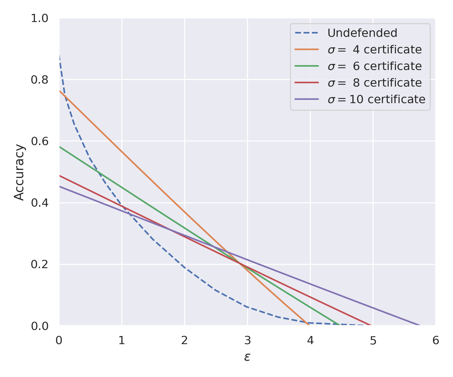
(b) Human activity recognition

Figure 3: Certificates against online adversarial attacks for varying smoothing noises. Here we can perturb each input only once. The average size of perturbation is computed as per equation 2.

We test our certificates for two streaming tasks – speech keyword detection and human activity recognition. We use a subset of the Speech commands dataset (Warden, 2018) for our speech keyword detection task. The subset we use contains ten keyword classes, corresponding to utterances of numbers from zero to nine recorded at a sample rate of 16 kHz. This dataset also contains noise clips such as audio of running tap water and exercise bike. We add these noise clips to the speech audio to simulate real-world scenarios and stitch them together to generate longer audio clips. We use the UCI HAR dataset (Reyes-Ortiz et al., 2012) for human activity recognition. This contains a 6-D triaxial accelerometer and gyroscope readings measured with human subjects. The objective in HAR is to recognize various human activities based on sensor readings. The UCI HAR dataset contains signals recorded at 50 Hz that correspond to six human activities such as standing, sitting, laying, walking, walking up, and walking down.

We use the M5 network described in (Dai et al., 2017) with an SGD optimizer and an initial learning rate of 0.1, which we anneal using a cosine scheduler. For the speech detection task, we train a M5 network with 128 channels for 30 epochs with a batch size of 128. For the human activity recognition task, we use a M5 network with 32 channels for 30 epochs with a batch size of 256. We apply isotropic Gaussian noise for smoothing and use the $\ell_{2}$-norm to define the average distance measure $d$. For the speech keyword detection task, we use smoothing noises with standard deviations of 0.1, 0.2, 0.4, 0.6, and 0.8. For the human activity recognition task, we use smoothing noises with standard deviations of 4, 6, 8, and 10. See Appendix E for more details on the experiments. We compute certificates for both scenarios, where the input is attacked only once and where each window can be attacked with the ability to re-attack inputs. These experiments show that our certificates provide meaningful guarantees against adversarial perturbations.

Algorithm 1 Our streaming attack

  Input: time-step $j$, clean inputs $x_{j},x_{j-1},...,x_{j-w+1}$, perturbed inputs $x^{\prime}_{j-1},...,x^{\prime}_{j-w+1}$, attack budget $\epsilon$, search parameter $\alpha\in\mathbb{N}$.

  $d_{j-1}=\sum_{i=1}^{j-1}d(x_{i},x_{i}^{\prime})$

  $budget_{j}=j\epsilon-d_{j-1}$

  for $i=0$ to $\alpha$ do

     $\epsilon^{\prime}=\frac{i}{\alpha}\cdot budget_{j}$

     $x=\arg\min_{x}f_{j}(x,...,x_{j-w+1}^{\prime})$ s.t. $d(x,x_{j})\leq\epsilon^{\prime}$

     if $f_{j}(x_{j}^{\prime},...,x_{j-w+1}^{\prime})=0$ then

        $x_{j}^{\prime}=x$

        break

     else

        $x_{j}^{\prime}=x_{j}$

     end if

  end for

6.1 Attacking an input only once

(a) Speech keyword detection

(b) Human activity recognition

Figure 4: Best certificates across varying smoothing noises for different window sizes. Streaming models with smaller window sizes are more robust to adversarial perturbations.

(a) Speech keyword detection

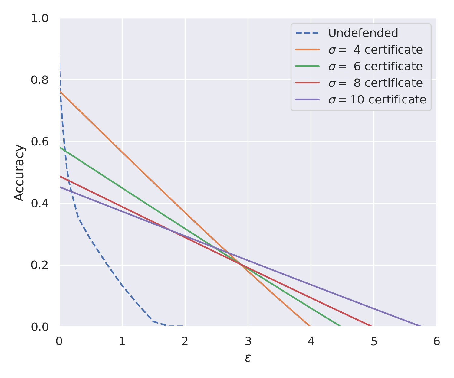
(b) Human activity recognition

Figure 5: Certificates against online adversarial attacks for varying smoothing noises. Here we attack each window with the ability to re-attack inputs. The average size of perturbation is computed as per equation 3.

We evaluate the robustness of undefended models using a custom-made attack that is constrained by the $\ell_{2}$-norm budget, as described in equation 2. To adhere to this constraint at each time-step $j$, the attacker must only perturb the input $x_{j}$, since the previous inputs $(x_{j-w+1},...,x_{j-1})$ have already been perturbed. This creates a significant challenge in creating a strong adversary. We design an adversary that only perturbs the last input $x_{j}$ at every time-step $j$ using projected gradient descent to minimize $f_{j}$. In our experiments, we set $f_{j}=1$ if the model outputs the correct class and $f_{j}=0$ when the model misclassifies. We linearly search using grid search parameter $\alpha$ for the smallest distance $d(x_{j},x_{j}^{\prime})$ such that the input $(x_{j-w+1}^{\prime},...,x_{j}^{\prime})$ leads to a misclassification at time-step $j$. We perturb $x_{j}$ if $(x_{j-w+1}^{\prime},...,x_{j}^{\prime})$ leads to misclassification and the average distance budget at time-step $j$ is less than $\epsilon$. Else, we do not perturb $x_{j}$. In this manner, our attack perturbs the streaming input in a greedy fashion. See Algorithm 1 for details.

We conduct our streaming attack on the keyword recognition task with a window size of $w=2$, where each input $x_{j}$ is a 4000-dimensional vector in the range [0,1]. We also perform the attack on the human activity recognition task with $w=2$, where each input $x_{j}$ is a 250x6-dimensional matrix. We use search parameter $\alpha=15$. We plot the results of our certificates for various smoothing noises (see Figure 3). Note that the attack budget $\epsilon$ is calculated as per the definition in equation 2. In Figure 4, we also plot our best certificates across various smoothing noises for different window sizes $w$. This plot supports our theory that streaming models with smaller window sizes are more robust to adversarial perturbations. Figures 7 and 8 in Appendix F show that the empirical performance of smooth models after the online adversarial attack is lower bound by our certificates. These plots validate our certificates.

6.2 Attacking each window

Now, we perform experiments for the attack setting described in Section 5. Note that here we need to calculate the attack budget $\epsilon$ based on equation 3. In this setting, we can re-attack an input for every window, making it a stronger attack. To attack the undefended models, we search for window perturbations that lead to misclassification using a minimum distance budget. Similar to our previous attack in Section 6.1, we only perturb a window at time-step $j$ if the average window distance at time-step $j$ is less than $\epsilon$. Also, we do not perturb a window if the window can not be perturbed to reduce the performance $f_{j}$. In Figure 5, we plot our certificates for this attack setting along with the accuracy of the undefended model for different attack budgets. These experiments show that our certificates produce meaningful performance guarantees against adversarial perturbations even if an attacker has the ability to re-attack the inputs. Figure 9 in Appendix F shows that the empirical performance of smooth models after the online adversarial attack is lower bound by our certificates. These plots validate our certificates.

7 Conclusion

In this work, we design provable robustness guarantees for streaming machine learning models with a sliding window. Our certificates provide a lower bound on the average performance of a streaming DNN model in the presence of an adversary. The adversarial budget in our threat model is defined in terms of the average size of the perturbations added to the input items across the entire stream. This allows the adversary to allocate a different budget to each input item and leads to a more general threat model than the static setting. Our certificates are independent of the stream length and can handle long, potentially infinite, streams. They are also applicable for adversaries that are allowed to re-attack past inputs leading to strong robustness guarantees covering a wide range of attack strategies.

Our robustness procedure simply augments the inputs with random noise. Unlike conventional randomized smoothing techniques, our method only requires one noised sample per prediction keeping the computational requirements of the DNN model unchanged. It does not make any assumptions about the DNN model such as Lipschitz continuity or a specific architecture and is applicable for conventional DNNs that are several layers deep. Our experimental results show that our certificates can obtain meaningful robustness guarantees for real-world streaming applications. Our results show that the certified performance of a robust model depends only on the window size and smaller windows lead to models that are provably more robust than larger windows.

To the best of our knowledge, this is the first attempt at designing adversarial robustness certificates for the streaming setting. We note that our robustness guarantees are not proven to be tight and could be improved upon by future work. We hope our work inspires further investigation into provable robustness methods for streaming ML models.

8 Acknowledgements

This project was supported in part by HR001119S0026 (GARD), NSF CAREER AWARD 1942230, ONR YIP award N00014-22-1-2271, Army Grant No. W911NF2120076, Meta grant 23010098, a capital one grant, NIST 60NANB20D134, and the NSF award CCF2212458.

Appendix A Proof of Lemma 5.1

Statement.

The change in each $\tilde{f}_{j}$ under an adversary in $\mathcal{A}_{\epsilon}$ is bounded as

$$|\tilde{f}_{j}(W_{j})-\tilde{f}_{j}(W_{j}^{\prime})|\leq\sum_{i=j-w+1}^{j}\psi(d(x_{i},x_{i}^{j+1-i})).$$

Proof.

The left-hand side of the above inequality can be re-written as:

$$|\tilde{f}_{j}(W_{j})-\tilde{f}_{j}(W_{j}^{\prime})| =|\tilde{f}_{j}(x_{j-w+1},\ldots,x_{j})-\tilde{f}_{j}(x_{j-w+1}^{w},\ldots,x_{j}^{1})|$$

$$=|\tilde{f}_{j}(x_{j-w+1},\ldots,x_{j-1},x_{j})-\tilde{f}_{j}(x_{j-w+1},\ldots,x_{j-1},x_{j}^{1})$$

$$+\tilde{f}_{j}(x_{j-w+1},\ldots,x_{j-1},x_{j}^{1})-\tilde{f}_{j}(x_{j-w+1}^{w},\ldots,x_{j-1}^{2},x_{j}^{1})|$$

$$=\Bigg{|}\sum_{k=1}^{w}\tilde{f}_{j}(x_{j-w+1},\ldots x_{j-k+1},x_{j-k+2}^{k-1},\ldots,x_{j}^{1})-\tilde{f}_{j}(x_{j-w+1},\ldots x_{j-k+1}^{k},x_{j-k+2}^{k-1},\ldots,x_{j}^{1})\Bigg{|}$$

$$\leq\sum_{k=1}^{w}\left|\tilde{f}_{j}(x_{j-w+1},\ldots x_{j-k+1},x_{j-k+2}^{k-1},\ldots,x_{j}^{1})-\tilde{f}_{j}(x_{j-w+1},\ldots x_{j-k+1}^{k},x_{j-k+2}^{k-1},\ldots,x_{j}^{1})\right|$$

The two terms in each summand differ only in the $(j-k+1)$-th input. Thus, it can be written as the difference of the expected value of some $[0,1]$-function $q$ under the distributions $\mathcal{S}(x_{j-k+1})$ and $\mathcal{S}(x_{j-k+1}^{k})$, i.e., $|\mathbb{E}_{\tilde{x}_{j-k+1}\sim\mathcal{S}(x_{j-k+1})}[q(\tilde{x}_{j-k+1})]-\mathbb{E}_{\tilde{x}_{j-k+1}^{k}\sim\mathcal{S}(x_{j-k+1}^{k})}[q(\tilde{x}_{j-k+1}^{k})]|$ which can be upper bounded by the total variation between $\mathcal{S}(x_{j-k+1})$ and $\mathcal{S}(x_{j-k+1}^{k})$. Therefore, from condition (4), we have:

$$|\tilde{f}_{j}(x_{j-w+1},\ldots, x_{j-k+1},x_{j-k+2}^{k-1},\ldots,x_{j}^{1})-\tilde{f}_{j}(x_{j-w+1},\ldots x_{j-k+1}^{k},x_{j-k+2}^{k-1},\ldots,x_{j}^{1})|$$

$$\leq\mathsf{TV}(\mathcal{S}(x_{j-k+1}),\mathcal{S}(x_{j-k+1}^{k}))\leq\psi(d(x_{j-k+1},x_{j-k+1}^{k})).$$

This proves the statement of the lemma. ∎

Appendix B Proof of Theorem 5.2

Statement.

Let $\tilde{Z}_{\epsilon}$ to be the minimum $\tilde{Z}$ for an adversary in $\mathcal{A}_{\epsilon}$. Then,

$$|\tilde{Z}-\tilde{Z}_{\epsilon}|\leq w\psi(\epsilon).$$

Proof.

Let $\tilde{Z}^{\prime}$ be the overall performance of $\tilde{M}$ under an adversary. Then,

$$|\tilde{Z}-\tilde{Z}^{\prime}| =\left|\frac{\sum_{j=1}^{t}\tilde{f}_{j}(W_{j})}{t}-\frac{\sum_{j=1}^{t}\tilde{f}_{j}(W_{j}^{\prime})}{t}\right|$$

$$\leq\frac{\sum_{j=1}^{t}|\tilde{f}_{j}(W_{j}))-\tilde{f}_{j}(W_{j}^{\prime})|}{t}$$

$$\leq\sum_{j=1}^{t}\sum_{k=1}^{w}\psi(d(x_{j-k+1},x_{j-k+1}^{k}))/t$$ (from lemma 5.1)

$$\leq\sum_{j=1}^{t}\sum_{k=1}^{w}\psi(d(x_{j},x_{j}^{k}))/t$$

$$=w\sum_{j=1}^{t}\sum_{k=1}^{w}\psi(d(x_{j},x_{j}^{k}))/wt$$

$$\leq w\psi\left(\sum_{j=1}^{t}\sum_{k=1}^{w}d(x_{j},x_{j}^{k}))/wt\right) \psi$$ ( is concave and Jensen’s inequality)

Therefore, for the worst-case adversary in $\mathcal{A}_{\epsilon}$, we have

$$|\tilde{Z}-\tilde{Z}_{\epsilon}|\leq w\psi(\epsilon)$$

from constraint (2) on the average distance between the original and perturbed inputs. ∎

Appendix C Function $\psi$ for Different Distributions

For an isometric Gaussian distribution,

$$\operatorname{\mathsf{TV}}(\mathcal{N}(x_{i},\sigma^{2}I),\mathcal{N}(x_{i}^{\prime},\sigma^{2}I))=\operatorname{erf}(\|x_{i}-x_{i}^{\prime}\|_{2}/2\sqrt{2}\sigma).$$

Proof.

Due to the isometric symmetry of the Gaussian distribution and the $\ell_{2}$-norm, the total variation between the two distributions is the same as when they are separated by the same $\ell_{2}$-distance but only in the first coordinate. It is equivalent to shifting a univariate normal distribution by the same amount. Therefore, the total variation between the two distributions is equal to the difference in the probability of a normal random variable with variance $\sigma^{2}$ being less than $\|x_{i}-x_{i}^{\prime}\|_{2}/2$ and $-\|x_{i}-x_{i}^{\prime}\|_{2}/2$, i.e., $\Phi(\|x_{i}-x_{i}^{\prime}\|_{2}/2\sigma)-\Phi(-\|x_{i}-x_{i}^{\prime}\|_{2}/2\sigma)$ where $\Phi$ is the standard normal CDF.

$$\operatorname{\mathsf{TV}}(\mathcal{N}(x_{i},\sigma^{2}I),\mathcal{N}(x_{i}^{\prime},\sigma^{2}I)) =\Phi(\|x_{i}-x_{i}^{\prime}\|_{2}/2\sigma)-\Phi(-\|x_{i}-x_{i}^{\prime}\|_{2}/2\sigma)$$

$$=2\Phi(\|x_{i}-x_{i}^{\prime}\|_{2}/2\sigma)-1$$

$$=2\left(\frac{1+\operatorname{erf}(\|x_{i}-x_{i}^{\prime}\|_{2}/2\sqrt{2}\sigma)}{2}\right)-1$$

$$=\operatorname{erf}(\|x_{i}-x_{i}^{\prime}\|_{2}/2\sqrt{2}\sigma).$$

∎

For a uniform smoothing distribution $\mathcal{U}(x_{i},b)$ between ${x_{i}}_{j}-b/2$ and ${x_{i}}_{j}+b/2$ in each dimension $j$ of $x_{i}$ for some $b\geq 0$, $\operatorname{\mathsf{TV}}(\mathcal{U}(x_{i},b),\mathcal{U}(x_{i}^{\prime},b))\leq\|x_{i}-x_{i}^{\prime}\|_{1}/b$. When $\|x_{i}-x_{i}^{\prime}\|_{1}$ is constrained, the overlap between $\mathcal{U}(x_{i},b)$ and $\mathcal{U}(x_{i}^{\prime},b)$ is minimized when the shift is only along one dimension.

Appendix D Comparison with Existing Certificates for Static Tasks

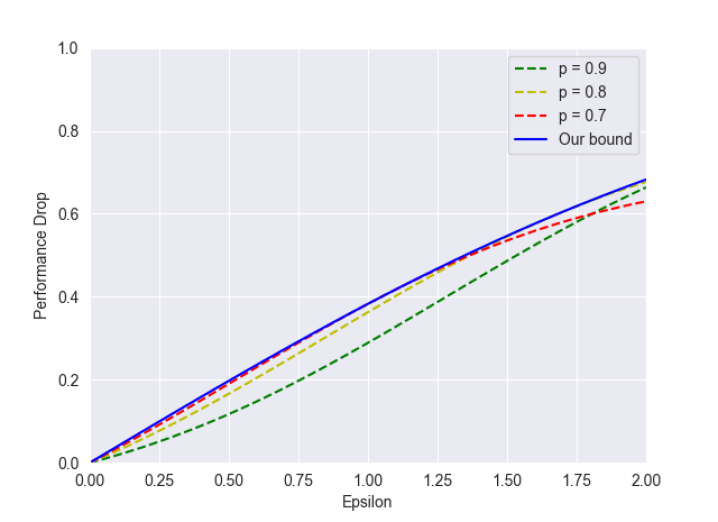
Figure 6: Comparison between our bound and Cohen et al. (2019)’s certificate for an $\ell_{2}$ adversary and a Gaussian smoothing distribution. The solid blue curve corresponds to our bound and the dashed curves represent bound (5) for different values of $p$. We keep $\sigma=1$ as it only has a scaling effect along the $x$-axis.

In this section, we compare our bound when applied to the static setting of classification, i.e., window size $w=1$ in bound (1), to that obtained by Cohen et al. (2019) for an $\ell_{2}$ adversary and a Gaussian smoothing distribution. As discussed in Appendix C, the $\psi$ function for this case takes the form of the Gauss error function $\operatorname{erf}$. Thus our bound on the drop in the smoothed model’s performance against an $\ell_{2}$ adversary is given by:

$$|\tilde{Z}-\tilde{Z}_{\epsilon}|\leq\operatorname{erf}(\epsilon/2\sqrt{2}\sigma).$$

Cohen et al. (2019)’s certificate bounds the worst-case adversarial performance as a function of the clean performance. If the probability of predicting the correct class is $p$ on the original input, the probability of that in the presence of an adversary is bounded by $\Phi(\Phi^{-1}(p)-\epsilon/\sigma)$. Therefore, the performance drop $\Delta p$ is bounded by:

$$\Delta p\leq p-\Phi\left(\Phi^{-1}(p)-\frac{\epsilon}{\sigma}\right).$$ (5)

Figure 6 compares the two bounds for different values of $p$. We keep $\sigma=1$ as it only has a scaling effect along the $x$-axis. The bound from the $\ell_{2}$ certificate by Cohen et al. (2019) is tighter than ours, mainly because it takes the clean performance $p$ of the smoothed model into account. However, the gap between the two bounds is small in the range where $\epsilon$ goes from 0 to 2, by which point the certified performance drops by more than 60%. Thus for most meaningful robustness guarantees, our certificates are almost at par with the best-known $\ell_{2}$ certificates. The key advantage of our certificates over those for the static setting is that they are applicable for an adaptive adversary that can allocate different attack budgets for different input items in the stream.

Appendix E Experimental details

We use a single NVIDIA RTX A4000 GPU with four AMD EPYC 7302P Processors. For our main experiments with UCI HAR and Speech Commands datasets, we use window size $w=2$ with inputs belonging to $\mathbb{R}^{250\times 6}$ and $\mathbb{R}^{4000}$. The UCI HAR dataset consists of long streaming inputs with sample-level annotations. For a window $W_{j}$, the label is the majority class that is present in that window. The signals in the HAR dataset are standardized to have mean 0 and variance 1. For the speech keyword detection task, we use a subset of the Speech commands dataset that consists of long noise clips and one-second-long speech keyword clips. The labels for each audio clip are available. We utilize all the long noise clips and clips belonging to the classes belonging speech utterances of numbers from zero to nine to make longer clips for our streaming case. We add noise clips to the keyword audios to make them more similar to real-world scenarios. Each clip is stitched together (Li et al., 2018) with arbitrarily long noise between each keyword clip. To make transitions between the audio smooth, we use exponential decays to overlap keyworrd audio clips for stitching, with noise in the background. Hence, for the speech keyword detection, we have 11 classes for labels – zero to nine and a noise class. A window is labeled to be the majority class in that window.

For training, we use M5 networks with 32 channels for HAR. We train for 30 epochs with a bath-size of 256 using SGD with an initial learning rate of 0.1, momentum of 0.9, and weight decay of 0.0001. We use a cosine annealing learning rate scheduler. For training the robust models, we use different smoothing noises with standard deviations 4, 6, 8, and 10. For training on the keyword detection data, we use M5 networks with 128 channels for HAR. We train for 30 epochs with a bath-size of 128 using SGD with an initial learning rate of 0.1, momentum of 0.9, and weight decay of 0.0001. We use a cosine annealing learning rate scheduler. For training the robust models, we use different smoothing noises with standard deviations 0.1, 0.2, 0.4, 0.6, and 0.8. For attacking the trained models, we use PGD $\ell_{2}$ attacks for both the datasets. PGD is run for 100 steps with a step size of $2\epsilon^{\prime}/100$ where $\epsilon^{\prime}$ is the $\ell_{2}$ attack budget.

Appendix F Attacking the Smooth Models

In this section, we empirically validate our certificates by showing that the performance of the smoothed models in the presence of an adversary is lower-bounded by our certificates. For the first set of experiments (Figures 7 and  8), we consider an adversary that is allowed to attack an input item only once, as in Section 6.1. We show our results on the Human Activity Recognition dataset in Figure 7 and the keyword detection task in Figure 8 for a window size of $w=2$. In Figure 9, we show our results on the HAR dataset where the adversary can attack each window separately as per equation 3. As seen in the plots, the empirical performance of the smooth models after the online adversarial attacks is always better than the performance guaranteed by our certificates. By comparing Figures 7 and 9, we observe that allowing the adversary to attack each window separately makes it significantly stronger and brings the adversarial performance of the smoothed model closer to the certified performance.

(a) Attacking model with smoothing noise $\sigma=4$

(b) Attacking model with smoothing noise $\sigma=6$

(c) Attacking model with smoothing noise $\sigma=8$

(d) Attacking model with smoothing noise $\sigma=10$

Figure 7: Certificates against online adversarial attacks for varying smoothing noises for the human activity recognition task. We attack smooth models trained with different smoothing noises in these plots. Here we can perturb each input only once. The average size of perturbation is computed as per equation 2.

(a) Attacking model with smoothing noise $\sigma=0.2$

(b) Attacking model with smoothing noise $\sigma=0.4$

(c) Attacking model with smoothing noise $\sigma=0.6$

(d) Attacking model with smoothing noise $\sigma=0.8$

Figure 8: Certificates against online adversarial attacks for varying smoothing noises for the speech keyword detection task. We attack smooth models trained with different smoothing noises in these plots. Here we can perturb each input only once. The average size of perturbation is computed as per equation 2.

(a) Attacking model with smoothing noise $\sigma=4$

(b) Attacking model with smoothing noise $\sigma=6$

(c) Attacking model with smoothing noise $\sigma=8$

(d) Attacking model with smoothing noise $\sigma=10$

Figure 9: Certificates against online adversarial attacks for varying smoothing noises for the human activity recognition task. We attack smooth models trained with different smoothing noises in these plots. Here we can attack each window separately. The average size of perturbation is computed as per equation 3.

References

- Athalye et al. (2018) Athalye, A., Carlini, N., and Wagner, D. Obfuscated gradients give a false sense of security: Circumventing defenses to adversarial examples. In Dy, J. and Krause, A. (eds.), Proceedings of the 35th International Conference on Machine Learning, volume 80 of Proceedings of Machine Learning Research, pp. 274–283, Stockholmsmässan, Stockholm Sweden, 10–15 Jul 2018. PMLR.
- Behzadan & Munir (2017) Behzadan, V. and Munir, A. Vulnerability of deep reinforcement learning to policy induction attacks. In Perner, P. (ed.), Machine Learning and Data Mining in Pattern Recognition - 13th International Conference, MLDM 2017, New York, NY, USA, July 15-20, 2017, Proceedings, volume 10358 of Lecture Notes in Computer Science, pp. 262–275. Springer, 2017. doi: 10.1007/978-3-319-62416-7“˙19. URL https://doi.org/10.1007/978-3-319-62416-7_19.
- Ben-Eliezer & Yogev (2020) Ben-Eliezer, O. and Yogev, E. The adversarial robustness of sampling. In Suciu, D., Tao, Y., and Wei, Z. (eds.), Proceedings of the 39th ACM SIGMOD-SIGACT-SIGAI Symposium on Principles of Database Systems, PODS 2020, Portland, OR, USA, June 14-19, 2020, pp. 49–62. ACM, 2020. doi: 10.1145/3375395.3387643. URL https://doi.org/10.1145/3375395.3387643.
- Ben-Eliezer et al. (2020) Ben-Eliezer, O., Jayaram, R., Woodruff, D. P., and Yogev, E. A framework for adversarially robust streaming algorithms. In Suciu, D., Tao, Y., and Wei, Z. (eds.), Proceedings of the 39th ACM SIGMOD-SIGACT-SIGAI Symposium on Principles of Database Systems, PODS 2020, Portland, OR, USA, June 14-19, 2020, pp. 63–80. ACM, 2020. doi: 10.1145/3375395.3387658. URL https://doi.org/10.1145/3375395.3387658.
- Biggio et al. (2013) Biggio, B., Corona, I., Maiorca, D., Nelson, B., Srndic, N., Laskov, P., Giacinto, G., and Roli, F. Evasion attacks against machine learning at test time. In Blockeel, H., Kersting, K., Nijssen, S., and Zelezný, F. (eds.), Machine Learning and Knowledge Discovery in Databases - European Conference, ECML PKDD 2013, Prague, Czech Republic, September 23-27, 2013, Proceedings, Part III, volume 8190 of Lecture Notes in Computer Science, pp. 387–402. Springer, 2013. doi: 10.1007/978-3-642-40994-3“˙25. URL https://doi.org/10.1007/978-3-642-40994-3_25.
- Bojarski et al. (2016) Bojarski, M., Testa, D. D., Dworakowski, D., Firner, B., Flepp, B., Goyal, P., Jackel, L. D., Monfort, M., Muller, U., Zhang, J., Zhang, X., Zhao, J., and Zieba, K. End to end learning for self-driving cars. CoRR, abs/1604.07316, 2016. URL http://arxiv.org/abs/1604.07316.
- Braverman et al. (2021) Braverman, V., Hassidim, A., Matias, Y., Schain, M., Silwal, S., and Zhou, S. Adversarial robustness of streaming algorithms through importance sampling. In Beygelzimer, A., Dauphin, Y., Liang, P., and Vaughan, J. W. (eds.), Advances in Neural Information Processing Systems, 2021. URL https://openreview.net/forum?id=83A-0x6Pfi_.
- Buckman et al. (2018) Buckman, J., Roy, A., Raffel, C., and Goodfellow, I. J. Thermometer encoding: One hot way to resist adversarial examples. In 6th International Conference on Learning Representations, ICLR 2018, Vancouver, BC, Canada, April 30 - May 3, 2018, Conference Track Proceedings, 2018.
- Cai et al. (2020) Cai, L., Gao, J., and Zhao, D. A review of the application of deep learning in medical image classification and segmentation. Annals of translational medicine, 8(11), 2020.
- Carlini & Wagner (2017) Carlini, N. and Wagner, D. A. Adversarial examples are not easily detected: Bypassing ten detection methods. In Proceedings of the 10th ACM Workshop on Artificial Intelligence and Security, AISec@CCS 2017, Dallas, TX, USA, November 3, 2017, pp. 3–14, 2017.
- Chiang et al. (2020) Chiang, P.-y., Ni, R., Abdelkader, A., Zhu, C., Studer, C., and Goldstein, T. Certified defenses for adversarial patches. In 8th International Conference on Learning Representations, 2020.
- Cohen et al. (2019) Cohen, J., Rosenfeld, E., and Kolter, Z. Certified adversarial robustness via randomized smoothing. In Chaudhuri, K. and Salakhutdinov, R. (eds.), Proceedings of the 36th International Conference on Machine Learning, volume 97 of Proceedings of Machine Learning Research, pp. 1310–1320, Long Beach, California, USA, 09–15 Jun 2019. PMLR.
- Dai et al. (2017) Dai, W., Dai, C., Qu, S., Li, J., and Das, S. Very deep convolutional neural networks for raw waveforms. In 2017 IEEE international conference on acoustics, speech and signal processing (ICASSP), pp. 421–425. IEEE, 2017.
- Datar & Motwani (2007) Datar, M. and Motwani, R. The Sliding-Window Computation Model and Results, pp. 149–167. Springer US, Boston, MA, 2007. ISBN 978-0-387-47534-9. doi: 10.1007/978-0-387-47534-9˙8. URL https://doi.org/10.1007/978-0-387-47534-9_8.
- Dennis et al. (2019) Dennis, D., Acar, D. A. E., Mandikal, V., Sadasivan, V. S., Saligrama, V., Simhadri, H. V., and Jain, P. Shallow rnn: Accurate time-series classification on resource constrained devices. In Wallach, H., Larochelle, H., Beygelzimer, A., d'Alché-Buc, F., Fox, E., and Garnett, R. (eds.), Advances in Neural Information Processing Systems, volume 32. Curran Associates, Inc., 2019. URL https://proceedings.neurips.cc/paper/2019/file/76d7c0780ceb8fbf964c102ebc16d75f-Paper.pdf.
- Dhillon et al. (2018) Dhillon, G. S., Azizzadenesheli, K., Lipton, Z. C., Bernstein, J., Kossaifi, J., Khanna, A., and Anandkumar, A. Stochastic activation pruning for robust adversarial defense. In 6th International Conference on Learning Representations, ICLR 2018, Vancouver, BC, Canada, April 30 - May 3, 2018, Conference Track Proceedings, 2018.
- Dvijotham et al. (2018) Dvijotham, K., Gowal, S., Stanforth, R., Arandjelovic, R., O’Donoghue, B., Uesato, J., and Kohli, P. Training verified learners with learned verifiers, 2018.
- Efroni et al. (2022) Efroni, Y., Jin, C., Krishnamurthy, A., and Miryoosefi, S. Provable reinforcement learning with a short-term memory. In Chaudhuri, K., Jegelka, S., Song, L., Szepesvári, C., Niu, G., and Sabato, S. (eds.), International Conference on Machine Learning, ICML 2022, 17-23 July 2022, Baltimore, Maryland, USA, volume 162 of Proceedings of Machine Learning Research, pp. 5832–5850. PMLR, 2022. URL https://proceedings.mlr.press/v162/efroni22a.html.
- Feigenbaum et al. (2005) Feigenbaum, J., Kannan, S., and Zhang, J. Computing diameter in the streaming and sliding-window models. Algorithmica, 41(1):25–41, 2005. doi: 10.1007/s00453-004-1105-2. URL https://doi.org/10.1007/s00453-004-1105-2.
- Fischer & Krauss (2018) Fischer, T. and Krauss, C. Deep learning with long short-term memory networks for financial market predictions. European Journal of Operational Research, 270(2):654–669, 2018. ISSN 0377-2217. doi: https://doi.org/10.1016/j.ejor.2017.11.054. URL https://www.sciencedirect.com/science/article/pii/S0377221717310652.
- Ganardi et al. (2019) Ganardi, M., Hucke, D., and Lohrey, M. Derandomization for sliding window algorithms with strict correctness. In van Bevern, R. and Kucherov, G. (eds.), Computer Science - Theory and Applications - 14th International Computer Science Symposium in Russia, CSR 2019, Novosibirsk, Russia, July 1-5, 2019, Proceedings, volume 11532 of Lecture Notes in Computer Science, pp. 237–249. Springer, 2019. doi: 10.1007/978-3-030-19955-5“˙21. URL https://doi.org/10.1007/978-3-030-19955-5_21.
- Gleave et al. (2020) Gleave, A., Dennis, M., Wild, C., Kant, N., Levine, S., and Russell, S. Adversarial policies: Attacking deep reinforcement learning. In 8th International Conference on Learning Representations, ICLR 2020, Addis Ababa, Ethiopia, April 26-30, 2020. OpenReview.net, 2020. URL https://openreview.net/forum?id=HJgEMpVFwB.
- Gong et al. (2017) Gong, Z., Wang, W., and Ku, W. Adversarial and clean data are not twins. CoRR, abs/1704.04960, 2017.
- Goodfellow et al. (2015) Goodfellow, I. J., Shlens, J., and Szegedy, C. Explaining and harnessing adversarial examples. In 3rd International Conference on Learning Representations, ICLR 2015, San Diego, CA, USA, May 7-9, 2015, Conference Track Proceedings, 2015.
- Gowal et al. (2018) Gowal, S., Dvijotham, K., Stanforth, R., Bunel, R., Qin, C., Uesato, J., Arandjelovic, R., Mann, T., and Kohli, P. On the effectiveness of interval bound propagation for training verifiably robust models, 2018.
- Graves & Schmidhuber (2005) Graves, A. and Schmidhuber, J. Framewise phoneme classification with bidirectional lstm and other neural network architectures. Neural Networks, 18(5):602–610, 2005. ISSN 0893-6080. doi: https://doi.org/10.1016/j.neunet.2005.06.042. URL https://www.sciencedirect.com/science/article/pii/S0893608005001206. IJCNN 2005.
- Grosse et al. (2017) Grosse, K., Manoharan, P., Papernot, N., Backes, M., and McDaniel, P. D. On the (statistical) detection of adversarial examples. CoRR, abs/1702.06280, 2017.
- Guo et al. (2018) Guo, C., Rana, M., Cissé, M., and van der Maaten, L. Countering adversarial images using input transformations. In 6th International Conference on Learning Representations, ICLR 2018, Vancouver, BC, Canada, April 30 - May 3, 2018, Conference Track Proceedings, 2018.
- Hsiao et al. (2020) Hsiao, R., Can, D., Ng, T., Travadi, R., and Ghoshal, A. Online automatic speech recognition with listen, attend and spell model. IEEE Signal Processing Letters, 27:1889–1893, 2020.
- Huang et al. (2019) Huang, P., Stanforth, R., Welbl, J., Dyer, C., Yogatama, D., Gowal, S., Dvijotham, K., and Kohli, P. Achieving verified robustness to symbol substitutions via interval bound propagation. In Proceedings of the 2019 Conference on Empirical Methods in Natural Language Processing and the 9th International Joint Conference on Natural Language Processing, EMNLP-IJCNLP 2019, Hong Kong, China, November 3-7, 2019, pp. 4081–4091, 2019. doi: 10.18653/v1/D19-1419. URL https://doi.org/10.18653/v1/D19-1419.
- Huang et al. (2017) Huang, S. H., Papernot, N., Goodfellow, I. J., Duan, Y., and Abbeel, P. Adversarial attacks on neural network policies. In 5th International Conference on Learning Representations, ICLR 2017, Toulon, France, April 24-26, 2017, Workshop Track Proceedings. OpenReview.net, 2017. URL https://openreview.net/forum?id=ryvlRyBKl.
- Ignatov (2018) Ignatov, A. Real-time human activity recognition from accelerometer data using convolutional neural networks. Applied Soft Computing, 62:915–922, 2018. ISSN 1568-4946. doi: https://doi.org/10.1016/j.asoc.2017.09.027. URL https://www.sciencedirect.com/science/article/pii/S1568494617305665.
- Janai et al. (2020) Janai, J., Güney, F., Behl, A., Geiger, A., et al. Computer vision for autonomous vehicles: Problems, datasets and state of the art. Foundations and Trends® in Computer Graphics and Vision, 12(1–3):1–308, 2020.
- Kamalaruban et al. (2020) Kamalaruban, P., Huang, Y.-T., Hsieh, Y.-P., Rolland, P., Shi, C., and Cevher, V. Robust reinforcement learning via adversarial training with langevin dynamics. In Larochelle, H., Ranzato, M., Hadsell, R., Balcan, M. F., and Lin, H. (eds.), Advances in Neural Information Processing Systems, volume 33, pp. 8127–8138. Curran Associates, Inc., 2020.
- Korczak & Hemes (2017) Korczak, J. and Hemes, M. Deep learning for financial time series forecasting in a-trader system. In 2017 Federated Conference on Computer Science and Information Systems (FedCSIS), pp. 905–912, 2017. doi: 10.15439/2017F449.
- Krauss et al. (2017) Krauss, C., Do, X. A., and Huck, N. Deep neural networks, gradient-boosted trees, random forests: Statistical arbitrage on the s&p 500. European Journal of Operational Research, 259(2):689–702, 2017. ISSN 0377-2217. doi: https://doi.org/10.1016/j.ejor.2016.10.031. URL https://www.sciencedirect.com/science/article/pii/S0377221716308657.
- Kumar & Goldstein (2021) Kumar, A. and Goldstein, T. Center smoothing: Certified robustness for networks with structured outputs. Advances in Neural Information Processing Systems, 34, 2021.
- Kumar et al. (2020) Kumar, A., Levine, A., Goldstein, T., and Feizi, S. Curse of dimensionality on randomized smoothing for certifiable robustness. In Proceedings of the 37th International Conference on Machine Learning, ICML 2020, 13-18 July 2020, Virtual Event, volume 119 of Proceedings of Machine Learning Research, pp. 5458–5467. PMLR, 2020. URL http://proceedings.mlr.press/v119/kumar20b.html.
- Kumar et al. (2021) Kumar, A., Levine, A., and Feizi, S. Policy smoothing for provably robust reinforcement learning. CoRR, abs/2106.11420, 2021. URL https://arxiv.org/abs/2106.11420.
- Kumar et al. (2022) Kumar, A., Levine, A., Goldstein, T., and Feizi, S. Certifying model accuracy under distribution shifts. CoRR, abs/2201.12440, 2022. URL https://arxiv.org/abs/2201.12440.
- Kurakin et al. (2017) Kurakin, A., Goodfellow, I. J., and Bengio, S. Adversarial machine learning at scale. In 5th International Conference on Learning Representations, ICLR 2017, Toulon, France, April 24-26, 2017, Conference Track Proceedings, 2017. URL https://openreview.net/forum?id=BJm4T4Kgx.
- Lécuyer et al. (2019) Lécuyer, M., Atlidakis, V., Geambasu, R., Hsu, D., and Jana, S. Certified robustness to adversarial examples with differential privacy. In 2019 IEEE Symposium on Security and Privacy, SP 2019, San Francisco, CA, USA, May 19-23, 2019, pp. 656–672, 2019.
- Lee et al. (2019) Lee, G., Nho, K., Kang, B., Sohn, K.-A., and Kim, D. Predicting alzheimer’s disease progression using multi-modal deep learning approach. Scientific reports, 9(1):1–12, 2019.
- Levine & Feizi (2021) Levine, A. and Feizi, S. Improved, deterministic smoothing for L1 certified robustness. CoRR, abs/2103.10834, 2021. URL https://arxiv.org/abs/2103.10834.
- Li et al. (2019) Li, B., Chen, C., Wang, W., and Carin, L. Certified adversarial robustness with additive noise. In Advances in Neural Information Processing Systems 32: Annual Conference on Neural Information Processing Systems 2019, NeurIPS 2019, 8-14 December 2019, Vancouver, BC, Canada, pp. 9459–9469, 2019.
- Li et al. (2018) Li, D., Langlois, T. R., and Zheng, C. Scene-aware audio for 360 videos. ACM Transactions on Graphics (TOG), 37(4):1–12, 2018.
- Li & Li (2017) Li, X. and Li, F. Adversarial examples detection in deep networks with convolutional filter statistics. In IEEE International Conference on Computer Vision, ICCV 2017, Venice, Italy, October 22-29, 2017, pp. 5775–5783, 2017.
- Madry et al. (2018) Madry, A., Makelov, A., Schmidt, L., Tsipras, D., and Vladu, A. Towards deep learning models resistant to adversarial attacks. In 6th International Conference on Learning Representations, ICLR 2018, Vancouver, BC, Canada, April 30 - May 3, 2018, Conference Track Proceedings, 2018.
- Mirman et al. (2018) Mirman, M., Gehr, T., and Vechev, M. Differentiable abstract interpretation for provably robust neural networks. In Dy, J. and Krause, A. (eds.), Proceedings of the 35th International Conference on Machine Learning, volume 80 of Proceedings of Machine Learning Research, pp. 3578–3586. PMLR, 10–15 Jul 2018. URL http://proceedings.mlr.press/v80/mirman18b.html.
- Mitrovic et al. (2017) Mitrovic, S., Bogunovic, I., Norouzi-Fard, A., Tarnawski, J., and Cevher, V. Streaming robust submodular maximization: A partitioned thresholding approach. In Guyon, I., von Luxburg, U., Bengio, S., Wallach, H. M., Fergus, R., Vishwanathan, S. V. N., and Garnett, R. (eds.), Advances in Neural Information Processing Systems 30: Annual Conference on Neural Information Processing Systems 2017, December 4-9, 2017, Long Beach, CA, USA, pp. 4557–4566, 2017. URL https://proceedings.neurips.cc/paper/2017/hash/3baa271bc35fe054c86928f7016e8ae6-Abstract.html.
- Mladenovic et al. (2022) Mladenovic, A., Bose, J., berard, H., Hamilton, W. L., Lacoste-Julien, S., Vincent, P., and Gidel, G. Online adversarial attacks. In International Conference on Learning Representations, 2022. URL https://openreview.net/forum?id=bYGSzbCM_i.
- Ordonez & Roggen (2016) Ordonez, F. J. and Roggen, D. Deep convolutional and lstm recurrent neural networks for multimodal wearable activity recognition. Sensors, 16(1), 2016. ISSN 1424-8220. doi: 10.3390/s16010115. URL https://www.mdpi.com/1424-8220/16/1/115.
- Ozbayoglu et al. (2020) Ozbayoglu, A. M., Gudelek, M. U., and Sezer, O. B. Deep learning for financial applications: A survey. Applied Soft Computing, 93:106384, 2020.
- Pattanaik et al. (2018) Pattanaik, A., Tang, Z., Liu, S., Bommannan, G., and Chowdhary, G. Robust deep reinforcement learning with adversarial attacks. In André, E., Koenig, S., Dastani, M., and Sukthankar, G. (eds.), Proceedings of the 17th International Conference on Autonomous Agents and MultiAgent Systems, AAMAS 2018, Stockholm, Sweden, July 10-15, 2018, pp. 2040–2042. International Foundation for Autonomous Agents and Multiagent Systems Richland, SC, USA / ACM, 2018. URL http://dl.acm.org/citation.cfm?id=3238064.
- Raghunathan et al. (2018) Raghunathan, A., Steinhardt, J., and Liang, P. Semidefinite relaxations for certifying robustness to adversarial examples. In Proceedings of the 32nd International Conference on Neural Information Processing Systems, NIPS’18, pp. 10900–10910, Red Hook, NY, USA, 2018. Curran Associates Inc.
- Reyes-Ortiz et al. (2012) Reyes-Ortiz, J., Anguita, D., Ghio, A., Oneto, L., and Parra, X. Uci machine learning repository: Human activity recognition using smartphones data set, 2012.
- Ronao & Cho (2016) Ronao, C. A. and Cho, S.-B. Human activity recognition with smartphone sensors using deep learning neural networks. Expert Systems with Applications, 59:235–244, 2016. ISSN 0957-4174. doi: https://doi.org/10.1016/j.eswa.2016.04.032. URL https://www.sciencedirect.com/science/article/pii/S0957417416302056.
- Salman et al. (2019) Salman, H., Li, J., Razenshteyn, I. P., Zhang, P., Zhang, H., Bubeck, S., and Yang, G. Provably robust deep learning via adversarially trained smoothed classifiers. In Advances in Neural Information Processing Systems 32: Annual Conference on Neural Information Processing Systems 2019, NeurIPS 2019, 8-14 December 2019, Vancouver, BC, Canada, pp. 11289–11300, 2019.
- Singla & Feizi (2019) Singla, S. and Feizi, S. Robustness certificates against adversarial examples for relu networks. CoRR, abs/1902.01235, 2019.
- Singla & Feizi (2020) Singla, S. and Feizi, S. Second-order provable defenses against adversarial attacks. In Proceedings of the 37th International Conference on Machine Learning, ICML 2020, 13-18 July 2020, Virtual Event, volume 119 of Proceedings of Machine Learning Research, pp. 8981–8991. PMLR, 2020. URL http://proceedings.mlr.press/v119/singla20a.html.
- Stamate et al. (2017) Stamate, C., Magoulas, G., Kueppers, S., Nomikou, E., Daskalopoulos, I., Luchini, M., Moussouri, T., and Roussos, G. Deep learning parkinson’s from smartphone data. In 2017 IEEE International Conference on Pervasive Computing and Communications (PerCom), pp. 31–40, 2017. doi: 10.1109/PERCOM.2017.7917848.
- Szegedy et al. (2014) Szegedy, C., Zaremba, W., Sutskever, I., Bruna, J., Erhan, D., Goodfellow, I. J., and Fergus, R. Intriguing properties of neural networks. In 2nd International Conference on Learning Representations, ICLR 2014, Banff, AB, Canada, April 14-16, 2014, Conference Track Proceedings, 2014.
- Tramer et al. (2020) Tramer, F., Carlini, N., Brendel, W., and Madry, A. On adaptive attacks to adversarial example defenses, 2020.
- Uesato et al. (2018) Uesato, J., O’Donoghue, B., Kohli, P., and van den Oord, A. Adversarial risk and the dangers of evaluating against weak attacks. In Proceedings of the 35th International Conference on Machine Learning, ICML 2018, Stockholmsmässan, Stockholm, Sweden, July 10-15, 2018, pp. 5032–5041, 2018.
- Vinitsky et al. (2020) Vinitsky, E., Du, Y., Parvate, K., Jang, K., Abbeel, P., and Bayen, A. M. Robust reinforcement learning using adversarial populations. CoRR, abs/2008.01825, 2020. URL https://arxiv.org/abs/2008.01825.
- Warden (2018) Warden, P. Speech Commands: A Dataset for Limited-Vocabulary Speech Recognition. ArXiv e-prints, April 2018. URL https://arxiv.org/abs/1804.03209.
- Wong & Kolter (2018) Wong, E. and Kolter, J. Z. Provable defenses against adversarial examples via the convex outer adversarial polytope. In Proceedings of the 35th International Conference on Machine Learning, ICML 2018, Stockholmsmässan, Stockholm, Sweden, July 10-15, 2018, pp. 5283–5292, 2018.
- Wu et al. (2021) Wu, F., Li, L., Huang, Z., Vorobeychik, Y., Zhao, D., and Li, B. CROP: certifying robust policies for reinforcement learning through functional smoothing. CoRR, abs/2106.09292, 2021. URL https://arxiv.org/abs/2106.09292.
- Xu et al. (2017) Xu, H., Gao, Y., Yu, F., and Darrell, T. End-to-end learning of driving models from large-scale video datasets. In 2017 IEEE Conference on Computer Vision and Pattern Recognition, CVPR 2017, Honolulu, HI, USA, July 21-26, 2017, pp. 3530–3538. IEEE Computer Society, 2017. doi: 10.1109/CVPR.2017.376. URL https://doi.org/10.1109/CVPR.2017.376.
- Yang et al. (2015) Yang, J. B., Nguyen, M. N., San, P. P., Li, X. L., and Krishnaswamy, S. Deep convolutional neural networks on multichannel time series for human activity recognition. In Proceedings of the 24th International Conference on Artificial Intelligence, IJCAI’15, pp. 3995–4001. AAAI Press, 2015. ISBN 9781577357384.
- Zhang et al. (2020) Zhang, H., Chen, H., Xiao, C., Li, B., Boning, D. S., and Hsieh, C. Robust deep reinforcement learning against adversarial perturbations on observations. CoRR, abs/2003.08938, 2020. URL https://arxiv.org/abs/2003.08938.
- Zhang et al. (2021) Zhang, H., Chen, H., Boning, D. S., and Hsieh, C.-J. Robust reinforcement learning on state observations with learned optimal adversary. In International Conference on Learning Representations, 2021. URL https://openreview.net/forum?id=sCZbhBvqQaU.
- Zhang et al. (2017) Zhang, L., Aggarwal, C., and Qi, G.-J. Stock price prediction via discovering multi-frequency trading patterns. In Proceedings of the 23rd ACM SIGKDD International Conference on Knowledge Discovery and Data Mining, KDD ’17, pp. 2141–2149, New York, NY, USA, 2017. Association for Computing Machinery. ISBN 9781450348874. doi: 10.1145/3097983.3098117. URL https://doi.org/10.1145/3097983.3098117.