Software implementation for calculating Chern and $\mathbb{Z}_{2}$ topological invariants of crystalline solids with WIEN2k all-electron density functional package

Abstract

We present two modules that expand functionalities of the all-electron full-potential density functional theory package WIEN2k for computation of the Chern and $\mathbb{Z}_{2}$ topological invariants. Characterization of topological properties relies on two methods: computing an evolution of hybrid Wannier charge centers for $\mathbb{Z}_{2}$ topological insulators (construction of maximally localized Wannier functions is not needed) and computing the Berry phase for a multitude of Wilson loops that discretize a 2D Brillouin zone for Chern insulators as well as for mapping the Berry curvature. The implementation is validated by testing on well-known materials that feature topologically non-trivial electronic states.

1 Introduction

Topological materials are new phases of matter outside the scope of Landau’s theory of phase transitions that have generated considerable interest due to their unusual electronic transport properties [1]. Topological materials led to a paradigm shift in the theoretical description of condensed matter. It becomes necessary to expand the band theory of solids by introducing new concepts, namely the Berry phase and curvature [2, 3], needed to explain observable physical phenomena, such as the quantum anomalous Hall (QAH) and quantum spin Hall (QSH) effects. Both topological phases (QAH and QSH) are associated with presence of an electronic bulk gap and gapless edge states [4, 5]. The QAH phase is related to a single spin conducting channel at the edge, while there are two channels (with opposite spins and group velocities) for the QSH phase [6]. These materials hold the potential for the development of innovative devices and applications in the emerging areas of quantum computing and spintronics [7, 8, 9].

Topological phases can be characterized by a global property of their electronic structure, i.e., a topological invariant [10]. The QAH phase in 2D systems with broken time reversal symmetry (TRS) is characterized by the total Chern number ($C$) given by [4], [11, chap. 3.2.2]

$$C=\frac{1}{2\pi}\sum_{n}^{\text{occ.}}\int_{\mathrm{BZ}}\mathbf{\Omega}^{(n)}(\mathbf{k})\cdot d\mathbf{S}.$$ (1)

Here the integral is taken over the whole Brillouin zone (BZ), $n$ is the band index (the summation runs over all occupied bands), and the integrand is a Berry curvature pseudovector. It is defined as ${\mathbf{\Omega}^{(n)}}(\mathbf{k})=\nabla_{\mathbf{k}}\times\mathcal{A}^{(n)}(\mathbf{k})$, where $\mathbf{k}$ is an electron wave vector and $\mathcal{A}^{(n)}(\mathbf{k})$ is the Berry potential $\mathcal{A}^{(n)}(\mathbf{k})=i\langle u_{\mathbf{k}}^{(n)}|\nabla_{\mathbf{k}}u_{\mathbf{k}}^{(n)}\rangle$ with $|u_{\mathbf{k}}^{(n)}\rangle$ being a cell-periodic part of the Bloch function. The Chern number is an integer that determines the value of QAH conductivity as $\sigma_{\text{QAH}}=C\,e^{2}/h$ [4], where $e$ and $h$ are the charge of the electron and Planck’s constant, respectively.

The Berry curvature ${\Omega}(\mathbf{k})$ is not readily available in practical density functional theory (DFT) calculations. This limitation precludes straightforward integration of Eq. (1). Instead, Soluyanov and Vanderbilt [12] proposed to evaluate the Chern number by tracking the evolution of hybrid Wannier charge centers (HWCCs) [13] from one boundary in the BZ ($k=0$) to its periodical image (e.g., $k=2\pi/a_{i}$)

$$C=\sum_{v}^{\text{occ.}}w^{(v)}(2\pi/a_{i})-\sum_{v}^{\text{occ.}}w^{(v)}(0).$$ (2)

Here $\mathbf{a}_{i}$ ($i=1,2,3$) are real space lattice vectors, $v$ is the Wannier function index (not to be confused with the band index, although the number of Wannier function for occupied states corresponds to the number of occupied bands). The HWCCs $w^{(v)}$ are calculated at discrete intermediate ($k=0\ldots 2\pi/a_{i}$) points in the BZ to ensure a smooth evolution of $\sum_{v}w^{(v)}(k)$ between boundaries due to the gauge uncertainty of $2\pi$ in the phase. Fractional coordinates for HWCCs are implied.

For the QSH phase Kane, Mele, and Fu proposed a $\mathbb{Z}_{2}$ invariant present in TRS 2D or 3D materials [14, 15]. As a consequence of TRS, the Bloch states are divided into Kramer’s pairs $|u_{\pm\mathbf{k},\alpha}^{I}\rangle$ and $|u_{\mp\mathbf{k},\alpha}^{II}\rangle$, where the $2N$ occupied bands are divided in $N$ pairs ($\alpha=1,\ldots,N$). Labels $I$ and $II$ distinguish the pairs such that under the TRS operation $\mathcal{T}$ they transform, up to a phase factor ($e^{i\theta_{k,\alpha}}$), as [16]

$$e^{i\theta_{k,\alpha}}\mathcal{T}|u_{\mathbf{k},\alpha}^{I}\rangle =|u_{-\mathbf{k},\alpha}^{II}\rangle,$$

$$-e^{i\theta_{-k,\alpha}}\mathcal{T}|u_{\mathbf{k},\alpha}^{II}\rangle =|u_{-\mathbf{k},\alpha}^{I}\rangle.$$ (3)

$\mathcal{T}$ is defined in terms of the spin ($S$) and complex conjugation ($K$) operators as $\mathcal{T}=e^{i\pi S/\hbar}K$. Each class of pairs has a corresponding Chern number $C_{I}$ and $C_{II}$ of equal magnitude but opposite in sign ($C_{I}=-C_{II}$). Thus, the total $C=C_{I}+C_{II}$ vanishes, resulting in a null Hall conductance [14]. Nevertheless, the $\mathbb{Z}_{2}$ invariant related to the Chern number as $\mathbb{Z}_{2}=|C_{I~{}\text{or}~{}II}|\mod 2$ allows us to distinguish between a trivial insulator and the QSH topological phase, which originates from the relativistic spin-orbit interaction. 2D materials are characterized by only one $\mathbb{Z}_{2}$ index; for the 3D case four independent indices are necessary [11, chap. 5.3.1], [15, 17]

$$\mathbb{Z}_{2}=(\nu_{0};\nu^{\prime}_{1}\nu^{\prime}_{2}\nu^{\prime}_{3}).$$ (4)

The so-called ‘weak’ indices $\nu^{\prime}_{1}$, $\nu^{\prime}_{2}$, and $\nu^{\prime}_{3}$ represent $|C_{I~{}\text{or}~{}II}|\mod 2$ invariants taken at three planes in reciprocal space cutting through time-reversal invariant momentum (TRIM) points at which $|u_{\mathbf{k},\alpha}^{I}\rangle=|u_{\mathbf{k},\alpha}^{II}\rangle$. The strong index $\nu_{0}$ differentiates between a weak and strong topological insulator [14, 15, 18]. The latter implies that metallic surface states are present on any exposed surface of the material [11, chap. 5.3.3].

Various methodologies for determining the $\mathbb{Z}_{2}$ topological invariant have been proposed [16, 19, 12, 20, 21]. The calculation of the surface states from first principles can be done, but it is cumbersome due to a great computational cost associated with the need of a super-cell construction. For the case of materials presenting inversion symmetry (IS), knowledge of the parity eigenvalues at TRIM points in the BZ is utilized [14]. Otherwise, for the general case of systems lacking this symmetry, a calculation can be done by integrating $\Omega(\mathbf{k})$ and $\mathcal{A}(\mathbf{k})$ over half of the Brillouin zone through an appropriate discretization method to avoid complications associated with the gauge fixing [16, 19, 20]. Soluyanov and Vanderbilt [20] analyzed obstructions associated with construction of Wannier functions for topological materials, which evolved into a practical approach for computing the $\mathbb{Z}_{2}$ indices by tracking the evolution of HWCCs in planes cutting through TRIM points in reciprocal space [21, 12]. The latter approach builds upon the concept of time-reversal polarization introduced by Liang and Kane [16] and became the most popular choice in ab initio calculations. Topological invariants are related to a gapless character of HWCCs as the wave vector evolves between TRIM points [21, 12, 20] (see section 2 for more details).

Z2Pack [22] and WannierTools [23] are open-source packages which offer numerical implementations for computing the aforementioned topological invariants. The Z2Pack accepts physical models based on an analytical Hamiltonian, a tight-binding Hamiltonian, or an input from ab initio DFT codes, such as VASP, Quantum ESPRESSO, and ABINIT. Those codes belong to the pseudopotential, plane-wave basis family. WannierTools, on the other hand, requires construction of a Wannier function tight-binding model based on the results obtained from an ab initio code via the Wannier90 package [24]. To the best of our knowledge, only one numerical implementations for computing the $C$ and $\mathbb{Z}_{2}$ topological invariants based on the all-electron full-potential DFT code has been reported so far [25]. Nonetheless, the program is not publicly available for use.

In this communication we introduce the implementation of two open-source programs that broaden the capability of the all-electron full-potential DFT package WIEN2k [26, 27] to the characterization of topological phases by computing both the $C$ and $\mathbb{Z}_{2}$ invariants. In addition to computing the topological invariants, this contribution allows us to generate a map of the Berry curvature $\Omega(\mathbf{k})$ in an arbitrary plane of the Brillouin zone, which can be employed for identifying regions with inhomogeneous $\Omega(\mathbf{k})$ values. The latter functionality complements the growing interest to direct experimental reconstruction of the Berry curvature in reciprocal space, which becomes a target for measuring an underlying topology of Bloch bands [28, 29, 30, 31, 32]. We employ the programs Wien2wannier [33] and BerryPI [34] for the calculation of overlap matrix elements and the Berry phase, respectively (both codes are implemented in WIEN2k). Our implementation does not require construction of Wannier functions thereby making characterization of topological materials more straightforward. This development complements the WloopPHI module [35] for characterization of Weyl semimetals and completes the set of tools for computational characterization of topological materials in the WIEN2k DFT package. Finally, the program was validated by computing topological invariants of a well-established $\mathbb{Z}_{2}$ topological insulator Bi2Se3 and a predicted Chern insulator FeBr3, as well as the Berry curvature map in monolayer MoS2.

2 Method

We consider the electronic ground-state for a periodic crystal, which is described by a single-particle mean-field Hamiltonian $H(\mathbf{k})$, which is a smooth function of the $\mathbf{k}$ crystalline wave vector. The eigenstates of this Hamiltonian are found through the solution of the Kohn-Sham equations given by the DFT [36, 37].

2.1 Hybrid Wannier charge centers

Our approach to computing HWCCs builds upon the method used in Z2Pack [22]. Figure 1a shows the construction of a string of $k$ points that form a closed loop (Wilson loop) due to periodicity of the BZ (i.e., equivalent initial and final $k$ points $\mathbf{k}_{1}\equiv\mathbf{k}_{J}$). The string is oriented along one of the reciprocal lattice vectors (the ‘Wannierization’ direction). The Wilson loop is discretized with $J$ points. All points on the string have a common $k_{i,\{1\}}$ coordinate (here $i$ is the point index, and the vector component index is in the curly brackets).

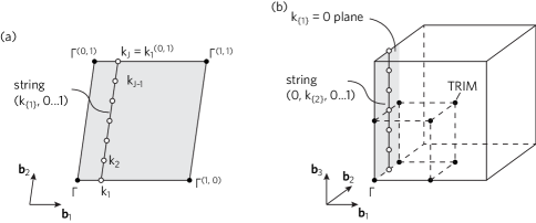
Figure 1: (a) String of $k$ points forming a Wilson loop in a 2D BZ used for calculation of HWCCs along direction of the second lattice vector. (b) The same construction in a 3D BZ for tracking of HWCCs along the third lattice vector and determination of $\mathbb{Z}_{2}$ indices. $k$ point coordinates are fractional in the basis of reciprocal lattice vectors $\mathbf{b}_{i}$ ($i=1,2,3$). The superscript indicates a periodic translation, e.g. $(0,1)$ implies translation along $\mathbf{b}_{2}$.

Overlap matrix elements are defined between the cell-periodic parts of two eigenstates as

$$S_{mn}(\mathbf{k}_{i},\mathbf{k}_{j})=\langle u^{(m)}_{\mathbf{k}_{i}}|u^{(n)}_{\mathbf{k}_{j}}\rangle\quad m,n\in[B_{\text{in}},B_{\text{fin}}].$$ (5)

Here $S$ is a square matrix with dimension given by the number of bands in the interval of interest $[B_{\text{in}},B_{\text{fin}}]$. A cumulative overlap matrix for the Wilson loop of $k$ points is expressed as the matrix product

$$M=\prod_{i=1}^{J-1}S(\mathbf{k}_{i},\mathbf{k}_{i+1}).$$ (6)

Note the equivalency $\mathbf{k}_{1}\equiv\mathbf{k}_{J}$ due to periodicity of the BZ (Fig. 1a). Eigenvalues of the cumulative overlap matrix

$$\lambda=\text{eig}(M)$$ (7)

are used to obtain HWCCs (fractional coordinates) from a complex argument of each eigenvalue

$$w_{\{\alpha\}}=\frac{\arg(\lambda)}{2\pi}\mod 1.$$ (8)

Here $\alpha\in\{1,2,3\}$ labels the direction of Wannierization (e.g., $w_{\{2\}}$ in Fig. 1a). It should not necessary be aligned with one of Cartesian directions ($x$, $y$, or $z$). Instead, the Wannierization direction is related to one of reciprocal lattice vector. For instance, if the Wannierization is performed along the first reciprocal lattice vector, the HWCCs will correspond to fractional coordinates along the first lattice vector in the real space. It should be emphasised that construction of maximally localized Wannier functions is not required when computing HWCCs.

2.2 Chern number

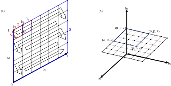
Figure 2: (a) Discretization of the BZ for the calculation of the Chern topological invariant. For each loop $S_{i}$ the Berry phase is calculated counterclockwise ($k_{1},..,k_{4},k_{1}$) and all the contributions are summed. The phase calculation direction consistency implies that the contributions from segments shared between two loops cancel each other, and the Berry phase for the boundary $\partial S$ is obtained. One of the Berry phase unwrapping schemes (horizontal) for adjacent k point loops is presented. The unwrapping starts from $\gamma_{2}$ with respect to $\gamma_{1}$ and follows the direction of the black arrow (a vertical scheme is also performed and a continuity criterion is checked for both). (b) Boundary (light blue) discretization of the BZ (light gray) at the selected plane with height $\lambda$.

For the calculation of the Chern number as per Eq. (1) it is necessary to perform an integration of the Berry curvature $\Omega(\mathbf{k})$ over the whole 2D BZ. In this context, the BZ is not taken as the Wigner-Seitz cell of the reciprocal space, but a primitive cell consisting of the parallelogram formed by the reciprocal lattice vectors as in Fig. 2. This integration can be performed by subdividing the 2D BZ (S) into patches ($\mathbf{S}_{i}$) such that the total Chern number is given by the sum of Berry phases $\gamma^{(n)}_{\partial S_{i}}$ of occupied states accumulated on the boundary of each patch as originally proposed by Fukui et al. [38]. The Berry phase is a $2\pi$ gauge-invariant quantity which represents a rotation in the complex phase of the cell-periodic part of the Bloch state $|u_{\mathbf{k}}^{(n)}\rangle$ as it traverses adiabatically a closed path over the BZ. It is defined in terms of the Berry potential $\mathcal{A}(\mathbf{k})$ and is related to the Berry curvature via Stoke’s theorem as

$$\gamma^{(n)}_{\partial S}=\oint_{\partial S}\mathcal{A}^{(n)}(\mathbf{k})\cdot d\mathbf{k}=\int_{S}{\mathbf{\Omega}^{(n)}}(\mathbf{k})\cdot d\mathbf{S},$$ (9)

where $\mathbf{S}$ is the vector of area normal to the surface, $S$ and $\partial S$ are the surface and its boundary, respectively. The calculation of the Chern number directly from ‘raw’ $\gamma_{\partial S}$ values is hindered by the gauge uncertainty. For instance, if we were to compute the Berry phase on the whole boundary $\partial S$ of the BZ, it would not be possible to differentiate between the phase of 0 and $2\pi$, or equivalently between the Chern number of 0 and 1. Therefore, an alternative approach involves dividing $S$ into subspaces $S_{i}$ sufficiently small, so that the obtained change in phase between adjacent loops $\partial S_{i}$ is smooth enough in comparison to the gauge uncertainty of $2\pi$. Thus, for a patch $\mathbf{S}_{i}$ we have the Berry phase expressed in terms of HWCCs (8) computed on a Wilson loop (Fig. 2a) comprised of discrete $k$ points [39]

$$\gamma_{\partial S_{i}}=2\pi\sum_{v}^{\text{occ.}}w^{(v)}\equiv\Phi_{i}.$$ (10)

This quantity is also referred to as a flux of Berry curvature (or the Berry flux) $\Phi_{i}$ through the patch. For a discrete grid, the magnitude of the Berry curvature pseudovector projection onto a normal $\hat{\mathbf{n}}$ to the plane $S_{i}$ can be approximated as

$$\mathbf{\Omega}(\mathbf{k})\cdot\hat{\mathbf{n}}_{S_{i}}\approx\frac{\gamma_{\partial S_{i}}}{S_{i}}.$$ (11)

Finally, the Chern number (1) is computed as [39, 38, 40, 41]

$$C=\frac{1}{2\pi}\sum_{i}^{\text{BZ}}\gamma_{\partial S_{i}}.$$ (12)

Since the Chern number is defined as the total flux of Berry curvature in the BZ, Eq. (12) can be viewed as a sum of locally calculated Berry fluxes through each patch, where the $i$ index runs over $\partial S_{i}$ in such way that the whole surface $\mathbf{S}$ is covered. The BZ constitutes a vectorial manifold, for the 2D case a $T^{2}$ torus, owing to the periodic boundary conditions of the crystal. Hence, the Chern number can be comprehended as the winding number of the Berry phase around this torus [18].

3 Program Implementation

3.1 Hybrid Wannier charge centers

It is implied that the user has converged an SCF calculation with SOC, and we continue to work in the same case directory. Calculation of HWCCs is managed by the wcc.py Python script, which is a part of the BerryPI package. The user needs to select the range of bands $[B_{\text{in}},B_{\text{fin}}]$, the Wannierization direction $\alpha$, the $k$ evolution direction and the range $k_{\text{evol}}\in[k_{\text{in}},k_{\text{fin}}]$, and fix the $k$ point coordinate in the remaining direction. For example, in Fig. 1b the Wilson loop is constructed along the third direction, the HWCCs evolution is recorded along the second direction $k_{\text{evol}}\in[0,0.5]$, and $k_{\text{fix}}=0$ in the first direction. The user also selects the number of points $J$ on the Wilson loop and the number of discretization intervals along the $k$ evolution direction. Sensible numbers are about 10 and 20, respectively, to begin with.

The main loop is performed over the $k_{\text{evol}}$ variable. For each value, a Wilson loop is constructed (one at a time) and corresponding fractional coordinates of $k$ points are stored in the case.klist file in a native WIEN2k format as three integer numbers per $k$ point with a common integer divisor. It is important to note conventions used within WIEN2k to interpret $k$ point coordinates in the case.klist file [26]. The BZ of a conventional lattice is implied for F, B, CXY, CXZ, and CXZ orthorhombic lattices. The BZ of a primitive lattice is used for other lattice types (P, H, R, CXZ monoclinic).

Once the case.klist file is set up, the script executes BerryPI to compute HWCCs for a given $k_{\text{evol}}$. Within BerryPI, the WIEN2k is called to compute wavefunctions for $k$ points on the Wilson loop followed by Wien2wannier to compute $S(\mathbf{k}_{i},\mathbf{k}_{i+1})$ overlap matrices between adjacent $k$ point on the loop. The $S(\mathbf{k}_{i},\mathbf{k}_{i+1})$ matrices are stored in the case.mmn file. Then, BerryPI reads the case.mmn file and computes HWCCs following Eqs. (6)-(8). The HWCCs $w_{\alpha}(k_{\text{evol}})$ are stored in a temporary wcc_i.csv file, which concludes one cycle. Data on the evolution of HWCCs are consolidated in the wcc.csv file as a function of $k_{\text{evol}}$.

Sample of wcc.csv listing with $w^{(v)}$ values defined by Eq. (8) for each Wilson loop stored in rows:

#k values are fractional coordinates in direction of the recip. latt. vec. G[2]
#WCC are evaluated on a Wilson loop in direction of the recip. latt. vec. G[3]
#k,WCC 1,WCC 2,WCC 3,WCC 4,WCC 5,WCC 6,WCC 7,...
0.000000,0.000000,0.000000,0.077836,0.077836,0.203946,0.203946,0.296585,...
0.026316,0.004659,0.004896,0.075512,0.078418,0.143604,0.233400,0.290768,...
0.052632,0.005981,0.013466,0.061571,0.080237,0.093847,0.246264,0.288668,...
0.078947,0.007861,0.020868,0.045604,0.079165,0.087893,0.251583,0.288239,...
0.105263,0.008441,0.023783,0.036129,0.077025,0.086447,0.257375,0.288128,...
0.131579,0.008095,0.023359,0.029160,0.075123,0.085686,0.264259,0.287875,...
0.157895,0.007344,0.021672,0.023798,0.073264,0.085003,0.270890,0.287507,...
...

Sample of wcc.py screen output that shows evolution of the total Berry phase $\sum_{v}w^{(v)}$ for each Wilson loop, which can be used to characterize Chern insulators:

Total Berry phase on each Wislon loop for bands 85-130:
------------------------------------------------------
 i           k            Phase wrap.    Phase unwrap.
                            (rad)           (rad)
------------------------------------------------------
 1  [***, 0.000, 0.000]     141.372           3.142
 2  [***, 0.026, 0.000]     141.544           3.314
 3  [***, 0.051, 0.000]     141.684           3.454
 4  [***, 0.077, 0.000]     141.780           3.550
...
39  [***, 0.974, 0.000]     147.482           9.252
40  [***, 1.000, 0.000]     147.655           9.425
------------------------------------------------------
Here "***" refer to the direction of the Wilson loop.

Users have an option to enable a parallel WIEN2k calculation (it requires setting up a .machines file [26]), add spin polarization, and an orbital potential (e.g., DFT+$U$). The SOC is enabled automatically.

3.2 Chern Number

CherN is a Python script that divides a plane $S$ in the BZ into subsets $S_{i}$ and evaluates the Berry phase for each boundary $\partial S_{i}$ following the method described in section 2 by recursively invoking the main BerryPI program. The script must be executed in the case directory after performing the standard WIEN2k self-consistent field calculation. For this purpose, the program receives as input: the band’s range [$B_{\text{in}},B_{\text{fin}}$], the plane normal direction and height, the boundary range [$b_{1}^{\text{initial}},b_{1}^{\text{final}},b_{2}^{\text{initial}},b_{2}^{\text{final}}$] (if $b_{3}$ is selected as the plane normal direction) and finally, the discretization parameters $n_{1}$ and $n_{2}$. For example, Fig. 2b presents a scenario for a plane in $b_{3}$ direction with height $\lambda$ and a boundary [$0,\alpha,0,\beta$]. It is worth noting that for the computation of the Chern number the boundary should cover the whole 2D BZ, i.e, $[0,1,0,1]$, and the band range selected should be separated from other bands by an energy gap (isolated individual band analysis can be performed). Moreover, it is possible to switch the spin-polarized, parallel, and orbital potential (DFT+$U$) calculation flags. SOC is implied by default.

Sample of CherN.py input:

    bands= [1,70]
    n_1 = 10
    n_2 = 10
    plane_dir = 3
    plane_height = 0.0
    boundary = [0,1.0,0,1.0]
    parallel = False
    spinpolar = True
    orbital = False

The script generates a mesh-grid discretization of $(n_{1}-1)\times(n_{2}-1)$ for the chosen boundary at a plane perpendicular to the selected direction and located at the constant height (see Fig. 2b). Following this, the program generates the appropriate case.klist file for each loop $\partial S_{i}$ in the discretized grid and invokes the BerryPI code with the specified flags. As the Berry phase calculation inherently carries a $2\pi$ uncertainty, two phase unwrapping schemes are utilized (the python numpy.unwrap function) for all the calculated phases (see Fig. 2b) to ensuring continuity of the Berry flux between adjacent patches. The acceptable criterion for continuity is $\Delta\gamma<\pi/2$ between any two adjacent patches. If the continuity criterion is not fulfilled, a warning message will be displayed at the end of the run. In the latter case it is imperative to increase the mesh grid ($n_{1},n_{2}$) until continuity is achieved. There is no a priori way to estimate values of the discretization parameters. In general, materials with a smaller gap require a denser mesh. According to a Kubo formula for the Berry curvature based on the perturbation theory (written as a sum over all states [42]), the Berry curvature is inversely proportional to the square of the energy difference between states. Thus, the curvature is more localized in materials with a smaller gap, especially near to band crossings [43, 44]. This fact should be taken as a marker for initial selection of the mesh density based on the band-structure analysis. Later we will give two examples of materials (MoS2 and FeBr3) and encourage the reader to verify this trend.

Finally, the program calculates the total Chern number $C$ by employing Eq. (12) and stores the result, as well as the Berry curvature projection data (image matrix with values in units of rad bohr² separated by comma) obtained from Eq. (11) in the berrycurv.dat file. This methodology differs from that chosen in the previously mentioned codes (Z2Pack and WannierTools) where Eq. (2) was employed, which implies the discretization of the Brillouin zone in a set of strings along the direction of one of the reciprocal lattice vectors. The two methods are equivalent from the Chern number perspective. In our case, however, the selection of loops also allow us to generate a map of the Berry curvature $\Omega(\mathbf{k})$ according to Eq. (11). If the Matplotlib library is installed, a Berry curvature map is saved in .png and .pdf formats. The source code of CherN is available in the BerryPI GitHub repository [45]. The execution of CherN requires WIEN2k [27] and BerryPI [34] (along with its dependencies) installed, as well as the NumPy library.

4 Validation

4.1 $\mathbb{Z}_{2}$ invariant in Bi2Se3 topological insulator

To validate the HWCCs implementation we compute invariants for Bi2Se3, the well-known topological insulator [46, 47]. The structure of Bi2Se3 (space group 166, $R\bar{3}m$ from Ref. 48) is shown in Fig. 3a (a conventional unit cell). The corresponding BZ (primitive cell) is depicted in Fig. 3b. Figure 3c presents the band structure of Bi2Se3 calculated in WIEN2k with SOC. It should be noted that SOC in WIEN2k is added perturbatively using a second variational method [49], and users need to be aware of the requirement to expand the basis set by adding empty states during the first scalar-relativistic step in LAPW1 (the default is 5 Ry above the Fermi energy, but materials with strong SOC may require 10 Ry [50, 26]). (Calculation parameters are: Perdew-Burke-Ernzerhof (PBE) [51] exchange-correlation functional; muffin tin radii $R_{\text{MT}}=2.5,2.47$ bohr for Bi and Se, respectively; 18 and 16 valence electrons for Bi and Se, respectively; $\min(R_{\text{MT}})K_{\text{max}}=8$; $5\times 5\times 5$ shifted k-mesh.) The obtained electronic structure corresponds to an insulator, but it is not possible to confirm the band inversion at $\Gamma$ due to SOC without an additional analysis.

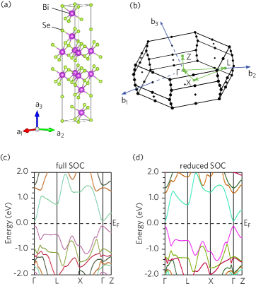
Figure 3: Bi2Se3: (a) conventional unit cell, (b) primitive Brillouin zone with the $k$ path (green), (c) band structure with SOC (full strength, a non-trivial topological phase), (d) band structure with a reduced SOC strength (a trivial insulator).

We investigate evolution of HWCCs between TRIM points using BerryPI/wcc.py in order to differentiate between a topologically trivial and non-trivial phase [21, 12]. For this purpose we selected a bundle of the 18 higher energy valence states. These states are well separated by a gap of ca. 3 eV from the remaining valence states. Results are shown in Fig. 4a,b. The panel (a) corresponds to HWCCs computed in a plane that starts at $\Gamma$ ($k_{1}=0,k_{2}=0$) and evolves towards L point ($k_{1}=0,k_{2}=0.5$), which is also one of TRIM points. The remaining dimension, i.e., the reciprocal lattice vector $\mathbf{b}_{3}$, is the Wannierization direction. The flow of HWCCs is gapless on panel (a). The panel (b) shows an evolution of HWCCs between another set of TRIM points L ($k_{1}=0.5,k_{2}=0$) and X ($k_{1}=0.5,k_{2}=0.5$). The HWCCs evolution becomes gaped when the plane passes away from $\Gamma$. We can conclude that the band inversion takes place at $\Gamma$ since the HWCCs evolution gap vanishes when approaching the center of the BZ indicating a non-trivial topological phase [12, 21]. This result is reminiscent of prior HWCCs calculations in Bi2Se3 (e.g., see Fig. 4 in Ref. 21 and Fig. 7 in Ref. 22). Adding more occupied states to the analysis will not change the outcome, but can obscure the flow (see Fig. 4 in Ref. 12 where 28 bands were used). It is worth mentioning that there is no exact mapping between band and HWCCs indices ($n\rightarrow v$) since more than one band generally contributes to one hybrid Wannier function. This information is contained in eigenvectors obtained when solving the eigenvalue problem (7). However, these eigenvectors are presently neither stored nor analyzed.

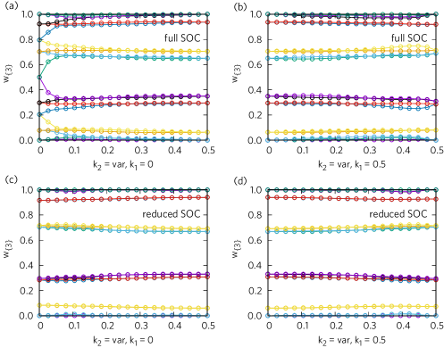
Figure 4: Evolution of HWCCs for Bi2Se3 in the BZ: (a,b) full SOC strength leads to a non-trivial topological insulator phase, (c,d) reduced SOC strength leads to a trivial insulator phase. HWCCs are derived from a bundle of 18 bands below the Fermi energy. Coordinates of $k$ points vary between TRIM points. The Wannierization direction is given in brackets $\{\ldots\}$.

To show a contrast between the non-trivial and trivial insulator phases we artificially adjusted the SOC strength in WIEN2k (LAPWSO module) by increasing the speed of light $c$ from ca. 137 to 300 at. units. Since the SOC strength is proportional to $c^{-2}$, the effective SOC was reduced by a factor of 4.8. At first glance, there are only minor visible changes to the band structure with reduced SOC (Fig. 3d). However, the flow of HWCCs changes drastically (Fig. 4c,d). The evolution of HWCCs becomes gaped also in the plane passing through $\Gamma$ indicating that this change in the SOC strength tunes Bi2Se3 away from the topological insulator phase as also noticed by Zhang et al. [46].

The gapless flow of HWCCs in an insulator (as in Fig. 4a) indicates winding of the HWCCs around the BZ, which is intimately connected with an adiabatic Thouless charge pumping in the bulk and leads to metallic edge states in a finite system [12, 16, 52, 53]. This bulk-boundary correspondence [54] is captured by topological invariants. The full set of $\mathbb{Z}_{2}$ topological indices can be inferred from the flow of HWCCs between various TRIM points [12]. In 3D time-reversal-invariant insulators we need HWCCs for the following set [11, chap. 5.3.1]

$$k_{1}=0,k_{2}=0\ldots 0.5,w_{\{3\}}\quad \text{and}\quad k_{1}=0.5,k_{2}=0\ldots 0.5,w_{\{3\}},$$ (13)

$$k_{1}=0\ldots 0.5,k_{2}=0,w_{\{3\}}\quad \text{and}\quad k_{1}=0\ldots 0.5,k_{2}=0.5,w_{\{3\}},$$ (14)

$$k_{2}=0,k_{3}=0\ldots 0.5,w_{\{1\}}\quad \text{and}\quad k_{2}=0.5,k_{3}=0\ldots 0.5,w_{\{1\}}.$$ (15)

Here the first (second) member in the set (13) is related to the $\nu_{1}$ ($\nu^{\prime}_{1}$) weak index. Panels (a) and (b) in Fig. 4 correspond to the set (13) leading to $\nu_{1}=1$ (gapless flow, one Wannier band is crossed when following the largest gap in the HWCC spectrum [12] as a function of $k_{2}$) and $\nu^{\prime}_{1}=0$ (gaped flow) indices, respectively. Results for the remaining two sets (14) and (15) are identical due to symmetry of the rhombohedral lattice and, therefore, are not shown. The remaining weak indices are $\nu_{2}=\nu_{3}=1$ and $\nu^{\prime}_{2}=\nu^{\prime}_{3}=0$. Since the flow of HWCCs is gapless in all directions originating at $\Gamma$, we should expect metallic states on any surface plane, hence the strong topological insulator ($\nu_{0}=1$) [12]. Following the definition (4), the complete topological invariant of Bi2Se3 is $\mathbb{Z}_{2}=(1;000)$, which is consistent with numerous prior studies [46, 12, 21].

4.2 Chern number of FeBr3

2D magnetic materials are profiled as appropriate systems to host the AHC topological phase. The intrinsic magnetic ordering fulfills the time-reversal symmetry-breaking condition and, as a result, conductive edge states are expected to appear in materials with non-trivial Chern numbers. Therefore, we validate our CherN module by employing it on the FeBr3 monolayer, reported as a hypothetical Chern insulator with a topological invariant value $|C|=1$ [55, 56, 57].

First, to obtain the FeBr3 monolayer structure we performed the ionic relaxation employing the VASP DFT package [58, 59]. The projector augmented wave pseudopotential (PAW) method [60, 61] was utilized with cut-off energy of 500 eV for the plane-wave basis. Pseudopoltentials with 8 and 7 valence electrons were selected for Fe and Br, respecively. The exchange and correlation functional used was the Perdew-Burke-Ernzerhof (PBE) [51] and the $\Gamma$-centered Monkhorst-Pack k-mesh grid [62] of $13\times 13\times 1$ was selected. Both the cell parameters and internal atomic positions were fully relaxed with a force criterion of less than $10^{-2}$ eV $\text{\AA}^{-1}$ on all atoms. Additionally, a vacuum of 20 Å was set to avoid inter-layer coupling. The obtained structure belongs to the $P\overline{3}$1m (162) space group and the optimized lattice parameter of $a=6.297~{}\text{\AA}$ is in good agreement with Ref. 57.

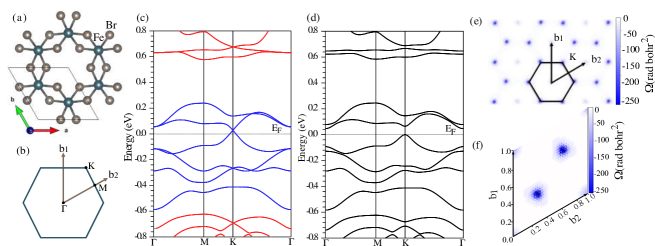
Figure 5: Monolayer FeBr3: (a) crystal structure, (b) BZ and high-symmetry points, (c,d) electronic band structure (spin-up:red, spin-down:blue) without and with SOC, respectively, (e) map of the Berry curvature pseudovector component $\Omega_{z}(\mathbf{k})$ in reciprocal space, (f) distribution of the Berry curvature pseudovector component $\Omega_{z}(\mathbf{k})$ in the primitive BZ (fractional coordinates).

The obtained structure was verified with the WIEN2k package to ensure that the atomic forces do not exceed 2 mRy bohr^-1 (ca. 0.05 eV Å^-1). Following this, the self-consistent field electronic structure calculation was performed within the spin-polarized and second-variational SOC framework, a parameter $\min(R_{\text{MT}})K_{\text{max}}=7$, and a k-point mesh grid of $15\times 15\times 1$ were taken. Here $K_{\text{max}}$ is the largest reciprocal-lattice vector size (plane wave cut-off), and atomic sphere radii are $R_{\text{MT}}$= 2.26, 2.15 bohr for Fe and Br, respectively. The energy cut-off separating the core from valence states was such that 14 and 17 electrons were considered as valence for Fe and Br, respectively. The calculation was initialized with a magnetic moment value of 1$\mu_{B}$ per formula unit, with Fe as the magnetically active atom, and the ground state found was ferromagnetic with a magnetic moment of 0.99$\mu_{B}$ per formula unit, henceforth, breaking the time-reversal symmetry of the system. Figure 5a,b shows the FeBr3 monolayer structure and the BZ, respectively. In Fig. 5c the electronic bandstructure without SOC is presented, where a crossing at the Fermi level (between bands 130 and 131) can be observed at the $K$ high-symmetry point. A SOC-induced gap opening of $47$ meV can be evidenced in Fig. 5d, which lifts the degeneracy at $E_{\text{F}}$ and may suggest the Chern insulator phase [55, 56, 57].

The projected Berry curvature map for FeBr3 is presented in Fig. 5e along with the detailed map in the primitive BZ (fractional coordinates) shown in Fig. 5f. It can be observed that the source of Berry curvature comes from the high symmetry point $K$ where the SOC gap emerged. The calculation was performed with the spin polar and parallel flags, the range of occupied bands $[1,130]$ was selected, and the discretization parameters $n_{1}=n_{2}=33$ were used. It should be noted that for obtaining reliable results these parameters must be increased until the continuity criterion is achieved, in this case for values higher than $n_{1}=n_{2}=21$ (higher values were employed for better graph resolution). Moreover, the lattice vector perpendicular to the monolayer ($\textbf{a}_{3}$) was selected as the plane_dir parameter, and the plane height was set to 0. The obtained Chern number given by Eq. (12) is $|C|=1$, which agrees with prior theoretical studies [55, 56, 57].

4.3 Berry curvature of MoS2

For the validation of the Berry curvature maps, the MoS2 monolayer was selected due to its characteristic behaviour, namely, the opposite Berry curvature at the corners of the hexagonal Brillouin zone ($K$ and $K^{\prime}$ high symmetry points as in Fig. 6b) [63, 64]. For this reason this material has attracted attention due to the potential uses in the emerging field of valleytronics [64, 65, 66, 67]. Nevertheless, as this is a non-magnetic monolayer the TRS breaking condition is not met, and it cannot be a Chern insulator ($C=0$).

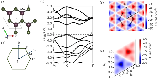
Figure 6: Monolayer MoS2: (a) crystal structure, (b) BZ, (c) calculated electronic band structure with SOC, (d) map of the Berry curvature pseudovector component $\Omega_{z}(\mathbf{k})$ in reciprocal space, (e) distribution of the Berry curvature pseudovector component $\Omega_{z}(\mathbf{k})$ in the primitive BZ (fractional coordinates).

The self-consistent field calculations were carried out with the full-potential linearized augmented plane-wave DFT method implemented in WIEN2k. The experimental data from Ref. 68 were utilized for the crystal structure, fixing the lattice parameter of the monolayer to $a_{1}=3.16~{}\text{\AA}$, which belongs to the $P\overline{6}m2$ (187) space group, as presented in Fig. 6a. To avoid interlayer coupling the distance between layers (center to center) was set at $a_{3}=12.3$ Å, which corresponds to the double value of interlayer distance in bulk. The PBE generalized gradient approximation [51] was selected for the exchange and correlation functional. For the electronic ground states the parameter $\min(R_{\text{MT}})K_{\text{max}}=7$ was utilized (muffin tin radii $R_{\text{MT}}=2.44,2.10$ bohr for Mo and S, respectively) with a k-mesh grid of $16\times 16\times 1$. The energy cut-off separating the core from valence states was such that 14 and 6 electrons were considered as valence for Mo and S, respectively; the charge leakage was checked. The spin-orbit coupling was taken into account.

The calculated ground state was found to be nonmagnetic (resulting in $|C|=0$), and the electronic band structure is presented in Fig. 6c. Here it can be seen that monolayer MoS2 is a semiconductor with a direct band gap of 1.8 eV [64]. For calculation of the Berry curvature map, the k-parallel flag was employed, the selected range of occupied bands was $[1,26]$, the selected plane_dir parameter corresponded to the lattice vector perpendicular to the monolayer (i.e., $\textbf{a}_{3}$), and the plane height was set to 0. The discretization parameters $n_{1}=n_{2}=51$ were selected, while the continuity of Berry curvature was achieved starting from $n_{1}=n_{2}=32$. The inherent inversion symmetry breaking due to the monolayer configuration combined with the strong SOC result in appearance of opposite sign contributions to the Berry curvature with peaks at the $K$ and $K^{\prime}$ high symmetry k-points. Moreover, $\Omega(\mathbf{k})$ vanishes at the $\Gamma$ and $M$ high symmetry points. These features of the Berry curvature map are in good agreement with prior theoretical studies by Feng et al. [63].

Data availability: All structure files, WIEN2k workflow and input sections for wcc.py and CherN.py required to reproduce results reported here are freely available from Zenodo repository [69].

5 Conclusion

We introduced two software modules for computing topological invariants from the density functional theory framework implemented in the all-electron full-potential package WIEN2k. Characterization of topological properties relies on computing an evolution of hybrid Wannier charge centers (for $\mathbb{Z}_{2}$ topological insulators) and Berry phase for a multitude of Wilson loops that discretize a 2D Brillouin zone (for Chern insulators and the Berry curvature map). Validation of the program was confirmed by testing on the well-known materials with topological features: Bi2Se3 as a $\mathbb{Z}_{2}$ topological insulator, monolayer FeBr3 as a Chern insulator, and monolayer MoS2 with a peculiar Berry curvature map. The acquired results agree with the available experimental and computational data. The analysis of topological characteristics can be performed directly after completing a self-consistent field calculation without constructing maximally localized Wannier functions. This feature makes these computational tools attractive for the study and prediction of topological materials especially in a high-throughput computational screening environment.

6 Acknowledgements

We thank to Peter Blaha (TU Vienna) for reading the manuscript and giving us constructive feedback. A.F.G.-B. would like to thank the MITACS organization for the financial support and logistics provided through the Globalink program. Calculations were performed using the Compute Canada infrastructure supported by the Canada Foundation for Innovation under John R. Evans Leaders Fund.

References

- Haldane [2017] D. Haldane. Nobel lecture: Topological quantum matter. Rev. Mod. Phys., 89:040502, 2017.
- Berry [1984] M. V. Berry. Quantal phase factors accompanying adiabatic changes. Proc. R. Soc. Lond. Series A, 392(1802):45–57, 1984.
- Zak [1989] J. Zak. Berry’s phase for energy bands in solids. Phys. Rev. Lett., 62:2747–2750, 1989.
- Thouless et al. [1982] D. Thouless, M. Kohmoto, M. Nightingale, and M. Nijs. Quantized Hall conductance in a two-dimensional periodic potential. Phys. Rev. Lett., 49:405–408, 1982.
- Haldane [1988] D. Haldane. Model for a quantum Hall effect without Landau levels: Condensed-matter realization of the "parity anomaly". Phys. Rev. Lett., 61:2015–2018, 1988.
- Liu et al. [2016] C. Liu, S. Zhang, and X. Qi. The quantum anomalous Hall effect: Theory and experiment. Annu. Rev. Condens. Matter Phys., 7:301–321, 2016.
- Hasan and Kane [2010] M. Z. Hasan and C. L. Kane. Colloquium: Topological insulators. Rev. Mod. Phys., 82:3045–3067, 2010.
- Ando [2013] Y. Ando. Topological insulator materials. J. Phys. Soc. Jpn., 82:1–32, 2013.
- Qi and Zhang [2011] X. Qi and S. Zhang. Topological insulators and superconductors. Rev. Mod. Phys., 83:1057–1110, 2011.
- Simon [2018] D. Simon. Tying light in knots: Applying topology to optics. Iop Concise Physics, 2018.
- Vanderbilt [2018] D. Vanderbilt. Chapter 5.3.1:topological index set. In Berry phases in electronic structure theory: Electric polarization, orbital magnetization and topological insulators. Cambridge University Press, Cambridge, England, 2018.
- Soluyanov and Vanderbilt [2011a] A. Soluyanov and D. Vanderbilt. Computing topological invariants without inversion symmetry. Phys. Rev. B, 83:235401, 2011a.
- Sgiarovello et al. [2001] C. Sgiarovello, M. Peressi, and R. Resta. Electron localization in the insulating state: Application to crystalline semiconductors. Phys. Rev. B, 64:115202, 2001.
- Kane and Mele [2005] C. L. Kane and E. J. Mele. topological order and the quantum spin Hall effect. Phys. Rev. Lett., 95:146802, 2005.
- Liang et al. [2007] F. Liang, C. L. Kane, and E. J. Mele. Topological insulators in three dimensions. Phys. Rev. Lett., 98:106803, 2007.
- Liang and Kane [2006] F. Liang and C. L. Kane. Time reversal polarization and a adiabatic spin pump. Phys. Rev. B, 74:195312, 2006.
- Fu and Kane [2007] L. Fu and C. L. Kane. Topological insulators with inversion symmetry. Phys. Rev. B, 76:045302, 2007.
- Bercioux et al. [2018] D. Bercioux, J. Cayssol, M.G. Vergniory, and C.M Reyes, editors. Topological matter:Lectures from the topological matter school 2017. Springer International Publishing, Basel, Switzerland, 1 edition, 2018.
- Fukui and Hatsugai [2007] T. Fukui and Y. Hatsugai. Quantum spin Hall effect in three dimensional materials: Lattice computation of topological invariants and its application to \ceBi and \ceSb. J. Phys. Soc. Jpn., 76(5):053702, 2007.
- Soluyanov and Vanderbilt [2011b] A. Soluyanov and D. Vanderbilt. Wannier representation of topological insulators. Phys. Rev. B, 83:035108, 2011b.
- Yu et al. [2011] R. Yu, X.Q. Liang, A. Bernevig, Z. Fang, and X. Dai. Equivalent expression of topological invariant for band insulators using the non-abelian Berry connection. Phys. Rev. B, 84:075119, 2011.
- Gresch et al. [2017] D. Gresch, G. Autès, O.V Yazyev, M. Troyer, D. Vanderbilt, B.A. Bernevig, and A. Soluyanov. Z2Pack: Numerical implementation of hybrid Wannier centers for identifying topological materials. Phys. Rev. B, 95:075146, 2017.
- Wu et al. [2018] Q. Wu, S. Zhang, H. Song, M. Troyer, and A. Soluyanov. WannierTools : An open-source software package for novel topological materials. Comput. Phys. Commun., 224:405 – 416, 2018.
- et al. [2020] G. Pizzi et al. Wannier90 as a community code: new features and applications. J. Phys. Condens. Matter, 32(16):165902, 2020.
- W.Feng et al. [2012] W.Feng, J. Wen, J. Zhou, D. Xiao, and Y. Yao. First-principles calculation of topological invariants within the fp-lapw formalism. Comput. Phys. Commun., 183(9):1849–1859, 2012.
- Blaha et al. [2018] P. Blaha, K. Schwarz, G.K.H. Madsen, D. Kvasnicka, J. Luitz, R. Laskowski, F. Tran, and L.D. Marks. WIEN2k: An augmented plane wave plus local orbitals program for calculating crystal properties. 2018.
- Blaha et al. [2020] P. Blaha, K. Schwarz, G.K.H. Madsen, D. Kvasnicka, J. Luitz, R. Laskowski, F. Tran, and L.D. Marks. WIEN2k: An apw+lo program for calculating the properties of solids. J. Chem. Phys., 152(7):074101, 2020.
- Mikitik and Sharlai [1999] G. P. Mikitik and Y.V. Sharlai. Manifestation of Berry’s phase in metal physics. Phys. Rev. Lett., 82:2147–2150, 1999.
- Liu et al. [2011] Y. Liu, G. Bian, T. Miller, and T.C Chiang. Visualizing electronic chirality and Berry phases in graphene systems using photoemission with circularly polarized light. Phys. Rev. Lett., 107:166803, 2011.
- Mikitik and Sharlai [2004] G. P. Mikitik and Y.V. Sharlai. Berry phase and de Haas-van Alphen effect in \ceLaRhIn5. Phys. Rev. Lett., 93:106403, 2004.
- Mak et al. [2014] K. F. Mak, K. L. McGill, J. Park, and P. L. McEuen. The valley Hall effect in \ceMoS2 transistors. Science, 344(6191):1489–1492, 2014.
- Liu et al. [2017] H. Liu, Y. Li, Y.S You, S. Ghimire, T.F Heinz, and D.A. Reis. High-harmonic generation from an atomically thin semiconductor. Nat. Phys., 13(3):262–265, 2017.
- Kuneš et al. [2010] J. Kuneš, R. Arita, P. Wissgott, A. Toschi, H. Ikeda, and K. Held. Wien2wannier: From linearized augmented plane waves to maximally localized Wannier functions. Comput. Phys. Commun., 181(11):1888–1895, 2010.
- Ahmed et al. [2013] S.J. Ahmed, J. Kivinen, B. Zaporzan, L. Curiel, S. Pichardo, and O. Rubel. BerryPI: A software for studying polarization of crystalline solids with WIEN2k density functional all-electron package. Comput. Phys. Commun., 184(3):647–651, 2013.
- Saini et al. [2022] H. Saini, M. Laurien, P. Blaha, and O. Rubel. WloopPHI: A tool for ab initio characterization of weyl semimetals. Comput. Phys. Commun., 270:108147, 2022.
- Hohenberg and Kohn [1964] P. Hohenberg and W. Kohn. Inhomogeneous electron gas. Phys. Rev., 136:B864–B871, 1964.
- Kohn and Sham [1965] W. Kohn and L. J. Sham. Self-consistent equations including exchange and correlation effects. Phys. Rev., 140:A1133–A1138, 1965.
- Fukui et al. [2005] T. Fukui, Y. Hatsugai, and H. Suzuki. Chern numbers in discretized brillouin zone: Efficient method of computing (spin) Hall conductances. J. Phys. Soc. Jpn., 74(6):1674–1677, 2005.
- Martin [2020] R.M. Martin. Electronic structure: Basic theory and practical methods. Cambridge University Press, Cambridge, England, 2 edition, 2020.
- Palyi et al. [2016] A. Palyi, J.K Asboth, and L. Oroszlany. A short course on topological insulators: Band structure and edge states in one and two dimensions. Springer International Publishing, Cham, Switzerland, 1 edition, 2016.
- de Paz et al. [2020] M. Blanco de Paz, C. Devescovi, G. Giedke, J.J Saenz, M.G Vergniory, B. Bradlyn, D. Bercioux, and A. García-Etxarri. Tutorial: Computing topological invariants in 2D photonic crystals. Adv. Quantum Technol., 3(2):1900117, 2020.
- Garg [2010] Anupam Garg. Berry phases near degeneracies: Beyond the simplest case. Amer. J. Phys., 78(7):661–670, 2010. 10.1119/1.3377135.
- Yao et al. [2004] Y. Yao, L. Kleinman, A.H MacDonald, J. Sinova, T. Jungwirth, D. Wang, E. Wang, and Q. Niu. First principles calculation of anomalous hall conductivity in ferromagnetic bcc fe. Phys. Rev. Lett., 92, 2004.
- Stejskal et al. [2022] O. Stejskal, M. Veis, and J. Hamrle. The flow of the berry curvature vector field. Sci. Rep., 12(1), 2022.
- Rubel [2022] O. Rubel. BerryPI: Software to study polarization and topological properties of crystalline solids. https://github.com/rubel75/BerryPI, 2022.
- Zhang et al. [2009] Haijun Zhang, Chao-Xing Liu, Xiao-Liang Qi, Xi Dai, Zhong Fang, and Shou-Cheng Zhang. Topological insulators in \ceBi2Se3, \ceBi2Te3 and \ceSb2Te3 with a single Dirac cone on the surface. Nat. Phys., 5(6):438–442, 2009.
- Xia et al. [2009] Y Xia, D Qian, D Hsieh, L Wray, A Pal, H Lin, A Bansil, D Grauer, Y S Hor, R J Cava, and M Z Hasan. Observation of a large-gap topological-insulator class with a single Dirac cone on the surface. Nat. Phys., 5(6):398–402, 2009.
- Nakajima [1963] S. Nakajima. The crystal structure of \ceBi2Te_3-xSe_x. J. Phys. Chem. Solids, 24(3):479–485, 1963.
- MacDonald et al. [1980] A. H. MacDonald, W. E. Picket, and D. D. Koelling. A linearised relativistic augmented-plane-wave method utilising approximate pure spin basis functions. J. Phys. C: Solid State Phys., 13(14):2675–2683, 1980. 10.1088/0022-3719/13/14/009.
- Kuneš et al. [2001] J. Kuneš, P. Novák, R. Schmid, P. Blaha, and K. Schwarz. Electronic structure of fcc Th: Spin-orbit calculation with 6 local orbital extension. Phys. Rev. B, 64(15):153102, 2001. 10.1103/physrevb.64.153102.
- Perdew et al. [1996] J.P. Perdew, K. Burke, and M. Ernzerhof. Generalized gradient approximation made simple. Phys. Rev. Lett., 77:3865–3868, 1996.
- Thouless [1983] D. J. Thouless. Quantization of particle transport. Phys. Rev. B, 27:6083–6087, 1983.
- Altshuler and Glazman [1999] B. L. Altshuler and L. I. Glazman. Pumping electrons. Science, 283(5409):1864–1865, 1999.
- Hatsugai [1993] Y. Hatsugai. Chern number and edge states in the integer quantum Hall effect. Phys. Rev. Lett., 71:3697–3700, 1993.
- Olsen et al. [2019] T. Olsen, E. Andersen, T. Okugawa, D. Torelli, T. Deilmann, and K.S Thygesen. Discovering two-dimensional topological insulators from high-throughput computations. Phys. Rev. Materials, 3:024005, 2019.
- Li [2019] P. Li. Prediction of intrinsic two dimensional ferromagnetism realized quantum anomalous Hall effect. Phys. Chem. Chem. Phys., 21:6712–6717, 2019.
- Zhang and Liu [2017] S.H. Zhang and B.G Liu. Intrinsic 2D ferromagnetism, quantum anomalous Hall conductivity, and fully-spin-polarized edge states of \ceFeBr3 monolayer, 2017.
- Kresse and Hafner [1993] G. Kresse and J. Hafner. Ab initio molecular dynamics for liquid metals. Phys. Rev. B, 47:558–561, 1993.
- Kresse and Furthmüller [1996] G. Kresse and J. Furthmüller. Efficiency of ab-initio total energy calculations for metals and semiconductors using a plane-wave basis set. Comput. Mater. Sci., 6(1):15–50, 1996.
- Blöchl [1994] P. E. Blöchl. Projector augmented-wave method. Phys. Rev. B, 50:17953–17979, 1994.
- Kresse and Joubert [1999] G. Kresse and D. Joubert. From ultrasoft pseudopotentials to the projector augmented-wave method. Phys. Rev. B, 59:1758–1775, 1999.
- Monkhorst and Pack [1976] H.J. Monkhorst and J.D Pack. Special points for Brillouin-zone integrations. Phys. Rev. B, 13:5188–5192, 1976.
- Feng et al. [2012] W. Feng, Y. Yao, W. Zhu, J. Zhou, W. Yao, and D. Xiao. Intrinsic spin Hall effect in monolayers of group-VI dichalcogenides: A first-principles study. Phys. Rev. B, 86:165108, 2012.
- Xiao et al. [2012] Di. Xiao, G.B Liu, W. Feng, X. Xu, and W. Yao. Coupled spin and valley physics in monolayers of \ceMoS2 and other group-VI dichalcogenides. Phys. Rev. Lett., 108:196802, 2012.
- Lembke et al. [2015] D. Lembke, S. Bertolazzi, and A. Kis. Single-layer \ceMoS2 electronics. Accounts Chem. Res., 48(1):100–110, 2015.
- Wang and Mi [2017] Z. Wang and B. Mi. Environmental applications of 2D molybdenum disulfide (\ceMoS2) nanosheets. Environ. Sci. Technol., 51(15):8229–8244, 2017.
- Li et al. [2014] H. Li, J. Wu, Z. Yin, and H. Zhang. Preparation and applications of mechanically exfoliated single-layer and multilayer \ceMoS2 and \ceWSe2 nanosheets. Accounts Chem. Res., 47(4):1067–1075, 2014.
- [68] \ceMoS2 crystal structure. https://materials.springer.com/isp/crystallographic/docs/sd_0309036.
- Gomez-Bastidas and Rubel [2023] A. F. Gomez-Bastidas and O. Rubel. Software implementation for calculating Chern and topological invariants with WIEN2k (workflows), 2023. URL https://zenodo.org/record/7761199. doi:10.5281/zenodo.7761198.