Non-planar corrections in orbifold/orientifold $\bm{\mathcal{N}=2}$ superconformal theories from localization

Abstract

We study non-planar corrections in two special $\mathcal{N}=2$ superconformal $SU(N)$ gauge theories that are planar-equivalent to $\mathcal{N}=4$ SYM theory: two-nodes quiver model with equal couplings and $\mathcal{N}=2$ vector multiplet coupled to two hypermultiplets in rank-2 symmetric and antisymmetric representations. We focus on two observables in these theories that admit representation in terms of localization matrix model: free energy on 4-sphere and the expectation value of half-BPS circular Wilson loop. We extend the methods developed in arXiv:2207.11475 to derive a systematical expansion of non-planar corrections to these observables at strong ’t Hooft coupling constant $\lambda$. We show that the leading non-planar corrections are given by a power series in $\lambda^{3/2}/N^{2}$ with rational coefficients. Sending $N$ and the coupling constant $\lambda$ to infinity with $\lambda^{3/2}/N^{2}$ kept fixed corresponds to the familiar double scaling limit in matrix models. We find that in this limit the observables in the two models are related in a remarkably simple way: the free energies differ by the factor of $2$, whereas the Wilson loop expectation values coincide. Surprisingly, these relations hold only at strong coupling, they are not valid in the weak coupling regime. We also discuss a dual string theory interpretation of the leading corrections to the free energy in the double scaling limit suggesting their relation to curvature corrections in type IIB string effective action.

1 Introduction and summary

Localization Pestun:2007rz ; Pestun:2016zxk is a remarkable tool that allows us to compute exactly various observables in conformal $\mathcal{N}=2$ supersymmetric 4d gauge theories (free energy on 4-sphere, circular half-BPS Wilson loop, correlation functions of chiral primary operators) in terms of special matrix models. It offers the possibility to study AdS/CFT correspondence beyond the planar limit and, in this way, understand better the structure of higher loop corrections in the dual string theory.

According to the standard AdS/CFT dictionary, (see, e.g., Aharony:1999ti )

$$g_{s}={\lambda\over 4\pi N}\,,\qquad\qquad T={L^{2}\over 2\pi\alpha^{\prime}{}}={\sqrt{\lambda}\over 2\pi}\,,$$ (1)

the expansion of observables in gauge theory in $1/N$ and, then, in inverse powers of large ’t Hooft coupling $\lambda\equiv g_{{}_{\small{\rm YM}}}^{2}N$ corresponds on the string side to expanding in string coupling $g_{s}\sim 1/N$ and, then, in the inverse string tension $T^{-1}\sim 1/\sqrt{\lambda}$. Within the localization approach, this expansion is well understood in maximally supersymmetric $SU(N)$ $\mathcal{N}=4$ Yang-Mills theory where the underlying matrix model is Gaussian (see, e.g., Erickson:2000af ; Drukker:2000rr ; Beccaria:2020ykg ; Beccaria:2021alk ). In $\mathcal{N}=2$ superconformal theories the localization matrix models contain nontrivial interaction potentials given by an infinite sum of single and double trace terms Pestun:2007rz ; Fiol:2015mrp ; Fiol:2020bhf ; Fiol:2020ojn . This makes the derivation of large $N$, large $\lambda$ expansion in these theories a non-trivial problem.

For the special class of superconformal $\mathcal{N}=2$ theories that are planar-equivalent to $\mathcal{N}=4$ SYM, the leading non-planar corrections to free energy and circular Wilson loop were studied using localization in a number of recent papers Beccaria:2020ykg ; Beccaria:2021ksw ; Beccaria:2021vuc ; Beccaria:2021ism ; Beccaria:2021hvt ; Beccaria:2022ypy ; Bobev:2022grf ; Beccaria:2022kxy . The aim of the present paper is to develop a systematical expansion of these observables beyond the leading order in $1/N$ and understand the properties of non-planar corrections at strong coupling. We shall consider two particular examples of $\mathcal{N}=2$ superconformal theories that we denote as $\mathsf{Q}_{2}$ and $\mathsf{SA}$ models.

The $\mathsf{Q}_{2}$ model is the $2-$node quiver $\mathcal{N}=2$ gauge theory (hence the name $\mathsf{Q}_{2}$) obtained as $\mathbb{Z}_{2}$ orbifold projection of the $SU(2N)$ $\mathcal{N}=4$ SYM. It describes an adjoint $SU(N)$ vector multiplet coupled to two $SU(N)\times SU(N)$ bi-fundamental $\mathcal{N}=2$ hypermultiplets with the same coupling constant. This model is dual to type IIB superstring on the orbifold ${\rm AdS}_{5}\times(S^{5}/\mathbb{Z}^{\rm orb}_{2})$ Kachru:1998ys ; Lawrence:1998ja ; Oz:1998hr ; Gukov:1998kk .

The $\mathsf{SA}$ model describes a vector multiplet coupled to two $\mathcal{N}=2$ hypermultiplets in the rank-2 symmetric and antisymmetric representations of the $SU(N)$ (hence the name $\mathsf{SA}$ for “symmetric-antisymmetric”). This theory may be viewed as an “orientifold” projection of the $\mathsf{Q}_{2}$ model. Its string theory dual is a special orientifold AdS${}_{5}\times(S^{5}/\Gamma)$, where $\Gamma=\mathbb{Z}_{2}^{\rm orb}\times\mathbb{Z}_{2}^{\rm orient}$ is the product of the orbifold projection and an orientifold action that, besides inversions of target space coordinates, also involves a product of world-sheet parity and $(-1)^{F_{L}}$ Park:1998zh ; Ennes:2000fu .

We shall mostly focus on computing the two important observables in these models – the free energy on the unit 4-sphere and the vacuum expectation value of a circular half-BPS Wilson loop. Due to the large $N$ planar equivalence, at leading order in $1/N$ these observables coincide with those of planar $\mathcal{N}=4$ SYM. The leading non-planar correction was found using the localization matrix model in Beccaria:2021ksw ; Beccaria:2021vuc ; Beccaria:2021hvt ; Beccaria:2022ypy ; Bobev:2022grf . Here we will compute the subleading non-planar corrections to the free energy and the circular Wilson loop in the $\mathsf{SA}$ and $\mathsf{Q}_{2}$ models and also discuss their interpretation on the dual string theory side.

Let us summarize our main results found from the corresponding localization matrix model.

Strong coupling expansion of free energy

The localization yields a matrix model representation of the partition function $Z(\lambda,N)$ of the $\mathsf{Q}_{2}$ and $\mathsf{SA}$ models on the 4-sphere. As these models are planar equivalent to $\mathcal{N}=4$ SYM, it is convenient to split their free energy $F(\lambda,N)=-\log Z(\lambda,N)$ into the sum of the free energy of the $SU(N)$ $\mathcal{N}=4$ SYM theory and the difference function

$$F^{\mathsf{SA}}(\lambda;N)=F^{\mathcal{N}=4}(\lambda;N)+\Delta F^{\mathsf{SA}}(\lambda;N)\,,$$

$$F^{\mathsf{Q}_{2}}(\lambda;N)=2F^{\mathcal{N}=4}(\lambda;N)+\Delta F^{\mathsf{Q}_{2}}(\lambda;N)\ ,$$

$$F^{\mathcal{N}=4}(\lambda;N)=-\frac{1}{2}(N^{2}-1)\log\lambda\,.$$ (2)

In the $\mathsf{Q}_{2}$ model, the $SU(N)$ $\mathcal{N}=4$ SYM contribution is doubled as in the planar limit each node of the quiver gives rise to $F^{\mathcal{N}=4}(\lambda;N)$.

In contrast to $F^{\mathcal{N}=4}(\lambda;N)$, the difference free energy $\Delta F(\lambda;N)$ remains finite at large $N$ and has the following expansion in powers of $1/N^{2}$

$$\Delta F(\lambda;N)=\mathsf{F}_{0}(\lambda)+\frac{1}{N^{2}}\mathsf{F}_{1}(\lambda)+\frac{1}{N^{4}}\mathsf{F}_{2}(\lambda)+\cdots\ .$$ (3)

As was mentioned above, the partition functions of the $\mathsf{SA}$ and $\mathsf{Q}_{2}$ models are given by the $SU(N)$ matrix model integrals containing the interaction potential given by an infinite sum of double traces of powers of the $SU(N)$ matrices. A peculiar feature of the interaction potential is that the double traces are accompanied by powers of the coupling constant. As a consequence, the weak coupling expansion of the difference free energy $\Delta F(\lambda;N)$ can be obtained by expanding the matrix integrals in powers of the interaction potential and evaluating them in a free Gaussian model.

For the same reason, the evaluation of $\Delta F(\lambda;N)$ at strong coupling becomes an extremely nontrivial problem because it requires taking into account an infinite number of terms in the interaction potential. For the leading term in (3), this leads to a representation of $\mathsf{F}_{0}(\lambda)$ as the determinant of a certain (model-dependent) semi-infinite matrix $K(\lambda)$. Early attempts to extract the strong coupling expansion of $\mathsf{F}_{0}(\lambda)$ used various approximations or numerical approaches in the $\mathsf{SA}$ model Beccaria:2021vuc ; Beccaria:2021hvt ; Bobev:2022grf and a numerical analysis Beccaria:2021ksw in the $\mathsf{Q}_{2}$ model.

Recently, it was observed Beccaria:2022ypy that the semi-infinite matrix $K(\lambda)$ in the $\mathsf{SA}$ model coincides with the matrix elements of the so called truncated (or temperature dependent) Bessel operator. It is interesting to note that this operator has previously appeared in the study of level spacing distributions in matrix models Tracy:1993xj and in the computation of four-point correlation functions of infinitely heavy half-BPS operators in planar $\mathcal{N}=4$ SYM Belitsky:2019fan ; Belitsky:2020qrm ; Belitsky:2020qir . Applying the methods developed in these papers, made it possible not only to compute the strong coupling expansion of $\mathsf{F}_{0}(\lambda)$ to any order in $1/\sqrt{\lambda}$ but also determine non-perturbative (exponentially suppressed) $O(e^{-\sqrt{\lambda}})$ corrections Beccaria:2022ypy .

Similarly, it was shown that in the $\mathsf{Q}_{2}$ model the matrix $K(\lambda)$ can be split into two irreducible blocks (associated with the untwisted and twisted sectors of states), whose determinants are captured by the extended Szegő-Akhiezer-Kac formula for the Fredholm determinant of the Bessel operator Beccaria:2022ypy .

The resulting strong coupling expansion of the leading term in (3) was found to be Beccaria:2022ypy

$$\mathsf{F}_{0}^{\mathsf{SA}}(\lambda)= \frac{1}{8}\lambda^{1/2}-\frac{3}{8}\log\lambda-3\log\mathsf{A}+\frac{1}{4}-\frac{11}{12}\log 2+{3\over 4}\log(4\pi)$$

$$+\frac{3}{32}\log{\lambda^{\prime}\over\lambda}-\frac{15\zeta(3)}{64\,{\lambda^{\prime}}^{3/2}}-\frac{945\zeta(5)}{512\,{\lambda^{\prime}}^{5/2}}-\frac{765\zeta(3)^{2}}{128\,{\lambda^{\prime}}^{3}}+O({\lambda^{\prime}}^{-7/2}),$$ (4)

$$\mathsf{F}_{0}^{\mathsf{Q}_{2}}(\lambda)= \frac{1}{4}\lambda^{1/2}-{1\over 2}\log\lambda-6\log\mathsf{A}+\frac{1}{2}-\frac{4}{3}\log 2+\log(4\pi)$$

$$+\frac{1}{16}\log{\lambda^{\prime}\over\lambda}-\frac{3\zeta(3)}{32\,{\lambda^{\prime}}^{3/2}}-\frac{135\zeta(5)}{256\,{\lambda^{\prime}}^{5/2}}-\frac{99\zeta(3)^{2}}{64\,{\lambda^{\prime}}^{3}}+O({\lambda^{\prime}}^{-7/2}),$$ (5)

where $\mathsf{A}$ is the Glaisher constant and $\lambda^{\prime}{}^{1/2}\equiv\lambda^{1/2}-4\log 2$ is a shifted coupling constant. The rationale for redefining the expansion parameter $\lambda\to\lambda^{\prime}$ is that it allows us to perform a resummation of all terms with coefficients containing powers of $\log 2$. Let us note that in the $\mathsf{Q}_{2}$ model (5) the coefficient of the leading $O(\lambda^{1/2})$ term is doubled as compared to the $\mathsf{SA}$ one in (4) (just like the planar $O(N^{2})$ contribution to the free energies $F^{\mathsf{Q}_{2}}$ and $F^{\mathsf{SA}}$ in (1)).

In this paper we extend the analysis of Beccaria:2022ypy and derive the strong coupling expansion of subleading non-planar corrections to (3). We show that in both models the functions $\mathsf{F}_{1}(\lambda),\mathsf{F}_{2}(\lambda),\dots$ in (3) are given by polynomials in the basic traces $\operatorname{\text{tr}}\big{[}RK(\lambda)/{\left({1-K(\lambda)}\right)}\big{]}$ involving again the leading-order matrix $K$ and some specific coupling-independent semi-infinite matrices $R$. We demonstrate that these traces can be expressed in terms of matrix elements of the resolvent of the Bessel operator mentioned above. We develop a technique for computing these matrix elements at strong coupling in a systematic way and, thus, find the corresponding expansions of coefficient functions in (3).

Explicitly, we find for the functions $\mathsf{F}_{1}$ and $\mathsf{F}_{2}$ in the $\mathsf{SA}$ model

$$\mathsf{F}_{1}^{\mathsf{SA}}(\lambda)={} -\frac{\lambda^{3/2}}{2048}-\frac{3\lambda}{2048}+\lambda^{1/2}\Big{(}\frac{11}{2048}-\frac{\log 2}{128}\Big{)}+\Big{(}\frac{3}{128}-\frac{\log^{2}2}{32}-\frac{\log 2}{512}\Big{)}$$

$$+{\frac{1}{\lambda^{1/2}}}\Big{(}-\frac{15\zeta(3)}{2048}-\frac{\log^{3}2}{8}-\frac{3\log^{2}2}{128}+\frac{279\log 2}{2048}\Big{)}$$

$$+{1\over\lambda}{\left({\frac{105\zeta(3)}{8192}-\frac{15\zeta(3)\log 2}{128}-\frac{\log^{4}2}{2}-\frac{5\log^{3}2}{32}+\frac{441\log^{2}2}{512}}\right)}+\dots,$$ (6)

$$\mathsf{F}_{2}^{\mathsf{SA}}(\lambda)={} \frac{\lambda^{3}}{2949120}-\frac{\lambda^{5/2}}{1310720}+\lambda^{2}\Big{(}\frac{\log 2}{61440}-\frac{251}{7864320}\Big{)}$$

$$+\lambda^{3/2}\Big{(}\frac{107}{3145728}+\frac{\log^{2}2}{15360}-\frac{47\log 2}{245760}\Big{)}$$

$$+\lambda\Big{(}\frac{409}{524288}+\frac{\zeta(3)}{65536}+\frac{\log^{3}2}{3840}-\frac{19\log^{2}2}{20480}-\frac{191\log 2}{262144}\Big{)}+\dots,$$ (7)

and for the function $\mathsf{F}_{1}$ in the $\mathsf{Q}_{2}$ model

$$\mathsf{F}_{1}^{\mathsf{Q}_{2}}(\lambda)= -\frac{\lambda^{3/2}}{1024}-\frac{\lambda}{3072}+\lambda^{1/2}\Big{(}\frac{5}{1024}-\frac{\log 2}{192}\Big{)}-\frac{\log^{2}2}{48}+\frac{\log 2}{256}$$

$$+\frac{1}{\lambda^{1/2}}\Big{(}-\frac{3\zeta(3)}{1024}-\frac{\log^{3}2}{12}+\frac{\log^{2}2}{64}+\frac{35\log 2}{1024}\Big{)}+\dots.$$ (8)

These expressions involve terms with powers of $\log 2$. Their resummation is less obvious than in the leading terms $\mathsf{F}_{0}^{\mathsf{SA}}(\lambda)$ in (4) and $\mathsf{F}_{0}^{\mathsf{Q}_{2}}(\lambda)$ in (5) and will be discussed below.

Double scaling limit

The obtained expressions for the non-planar corrections $\mathsf{F}_{0}(\lambda)$, $\mathsf{F}_{1}(\lambda)$ and $\mathsf{F}_{2}(\lambda)$ reveal an interesting structure. Namely, keeping only the leading large $\lambda$ terms in (4)–(8), we get for the corresponding $\Delta F$ in (3)

$$\Delta F^{\mathsf{SA}}(\lambda;N) =\frac{1}{8}\,\lambda^{1/2}-\frac{1}{N^{2}}\frac{\lambda^{3/2}}{2048}+\frac{1}{N^{4}}\frac{\lambda^{3}}{2949120}+\dots\,,$$

$$\Delta F^{\mathsf{Q}_{2}}(\lambda;N) =\frac{1}{4}\,\lambda^{1/2}-\frac{1}{N^{2}}\frac{\lambda^{3/2}}{1024}+\dots\,,$$ (9)

where dots stand for terms with subleading powers of $\lambda$ at each order in $1/N^{2}$. We observe that the coefficients of $1/N^{2}$ have increasing power of $\lambda$. The relation (9) suggests that in this limit (i.e. $N\to\infty$ and then $\lambda\to\infty$) the expansion of the free energy effectively runs in powers of $\lambda^{3/2}/N^{2}$. Moreover, we again observe that, as it happened at the $O(N^{2})$ and $O(N^{0})$ orders, the coefficients of the subleading $\lambda^{3/2}/N^{2}$ terms in (9) are again related by the factor of 2.

We shall argue that these properties can be understood as a consequence of the familiar double-scaling limit in the matrix models, see e.g. DiFrancesco:1993cyw ; Eynard:2015aea . In the present context it corresponds to the limit

$$N\to\infty\,,\qquad\lambda\to\infty\,,\qquad\ \frac{\lambda^{3/2}}{N^{2}}={\rm fixed}\,.$$ (10)

Taking this limit directly in the localization matrix model representation of the gauge theory partition function gives an efficient way of computing the coefficients of the leading large $\lambda$ terms in $\mathsf{F}_{n}$ in (3). By exploiting some recent results in the matrix models, we find that in the $\mathsf{SA}$ theory

$$\Delta F^{\mathsf{SA}}\simeq{} \frac{1}{8}\,\sqrt{\lambda}-\frac{1}{2048}\,\frac{\lambda^{3/2}}{N^{2}}+\frac{1}{2949120}\,\Big{(}\frac{\lambda^{3/2}}{N^{2}}\Big{)}^{2}-\frac{1}{1486356480}\,\Big{(}\frac{\lambda^{3/2}}{N^{2}}\Big{)}^{3}$$

$$-\frac{1}{304405807104}\,\Big{(}\frac{\lambda^{3/2}}{N^{2}}\Big{)}^{4}+\frac{17}{365286968524800}\,\Big{(}\frac{\lambda^{3/2}}{N^{2}}\Big{)}^{5}+\ldots\,,$$ (11)

where the sign ‘$\simeq$’ indicates that this relation is valid in the limit (10).

In addition, we prove that in the double scaling limit the free energies in the $\mathsf{SA}$ and $\mathsf{Q}_{2}$ models are related to each other as (to all orders in $1/N^{2}$)

$$\Delta F^{\mathsf{Q}_{2}}\simeq 2\Delta F^{\mathsf{SA}}\,.$$ (12)

We would like to emphasize that this relation is not satisfied at weak coupling. The appearance of this relation at strong coupling admits a possible interpretation on the string theory side as being a consequence of the fact that the $\mathsf{SA}$ model may be obtained from the $\mathsf{Q}_{2}$ one by an extra projection (see section 7).

The relation of (11) suggests that, in the double scaling limit (10), the difference free energy takes the following general form 

$$\Delta F\simeq c_{0}\sqrt{\lambda}+\sum_{n=1}^{\infty}c_{n}\Big{(}{\lambda^{3/2}\over N^{2}}\Big{)}^{n}=2\pi c_{0}T+\sum_{n=1}^{\infty}c_{n}\Big{(}8\pi{g^{2}_{s}\over T}\Big{)}^{n}\,,$$ (13)

where $c_{n}$ are rational coefficients. Here in the second relation we switched to the expansion parameters (1) of the dual string theory. We shall discuss the string theory interpretation of this expansion and coefficients $c_{n}$ in section 7 below.

Remarkably, a similar scaling behaviour was observed earlier in the strong coupling expansion of the circular Wilson loop in the $\mathcal{N}=4$ SYM theory in Drukker:2000rr (its dual $AdS_{5}\times S^{5}$ string-theory interpretation was given in Giombi:2020mhz ). However, in contrast to that case where the $(\lambda^{3/2}/N^{2})^{n}$ corrections to the Wilson loop exponentiated into $\exp(\lambda^{3/2}/(96N^{2}))=\exp(\pi{g^{2}_{s}/(12T)})$, here the series in (11) and (13) is likely to develop Borel singularities indicating the need to include non-perturbative, exponentially suppressed corrections.

Strong coupling expansion of circular Wilson loop

The expectation value of the half-BPS circular Wilson loop in the $\mathsf{SA}$ and $\mathsf{Q}_{2}$ models admits a representation in the localization matrix model similar to that for the free energy. Its large $N$ expansion in both models takes the form

$$N^{-1}{W}=\mathsf{W}_{0}+\frac{1}{N^{2}}\mathsf{W}_{1}+\frac{1}{N^{4}}\mathsf{W}_{2}+\cdots\,.$$ (14)

As for the free energy (1), the leading planar correction $\mathsf{W}_{0}$ is the same in the $\mathsf{SA}$ and $\mathsf{Q}_{2}$ models. It is equal to the planar term in the $SU(N)$ $\mathcal{N}=4$ SYM expression $\mathsf{W}_{0}=2{\sl I}_{1}(\sqrt{\lambda})/\sqrt{\lambda}$ where $I_{1}$ is a Bessel function Erickson:2000af ; Drukker:2000rr .

The deviation of $W$ from the exact $\mathcal{N}=4$ SYM result Drukker:2000rr in the $\mathsf{SA}$ and $\mathsf{Q}_{2}$ models starts at order $O(1/N^{2})$. It was observed in Beccaria:2021ksw ; Beccaria:2021vuc that at this order it is proportional to a derivative of the free energy with respect to the coupling constant. We found that a similar relation to the free energy holds also at higher orders of $1/N^{2}$ expansion. Namely, the ratios of the Wilson loop expectation values expanded in $1/N^{2}$ may be written as

$${{W}^{\mathsf{SA}}\over{W}^{\mathcal{N}=4}}= 1-\frac{\lambda^{2}}{4N^{2}}\,\mathsf{F}_{0}^{\prime}+\frac{1}{N^{4}}\,\Big{(}-\frac{\lambda^{3}}{48}\,\mathsf{F}_{0}^{\prime}+\frac{\lambda^{4}}{96}\,\mathsf{F}_{0}^{\prime}{}^{2}-\frac{\lambda^{4}}{96}\mathsf{F}_{0}^{\prime\prime}-\frac{\lambda^{3/2}}{4}\frac{{\sl I}_{2}(\sqrt{\lambda})}{{\sl I}_{1}(\sqrt{\lambda})}\,\mathsf{F}_{1}-\frac{\lambda^{2}}{4}\,\mathsf{F}_{1}^{\prime}\Big{)}+...$$

$${{W}^{\mathsf{Q}_{2}}\over{W}^{\mathcal{N}=4}}= 1-\frac{\lambda^{2}}{8N^{2}}\,\mathsf{F}_{0}^{\prime}+\frac{1}{N^{4}}\,\Big{(}-\frac{\lambda^{3}}{192}\,\mathsf{F}_{0}^{\prime}+\frac{\lambda^{4}}{384}\,\mathsf{F}_{0}^{\prime}{}^{2}-\frac{\lambda^{4}}{384}\mathsf{F}_{0}^{\prime\prime}-\frac{\lambda^{3/2}}{8}\frac{{\sl I}_{2}(\sqrt{\lambda})}{{\sl I}_{1}(\sqrt{\lambda})}\,\mathsf{F}_{1}-\frac{\lambda^{2}}{8}\,\mathsf{F}_{1}^{\prime}\Big{)}+\dots\,,$$ (15)

where $\mathsf{F}_{0}$ and $\mathsf{F}_{1}$ are the coefficients of the $1/N^{2}$ expansion (3) of the free energy $\Delta F^{\mathsf{SA}}$ and $\Delta F^{\mathsf{Q}_{2}}$ given by (4) – (8) and prime denotes derivative over $\lambda$. The leading $O(1/N^{2})$ terms in (1) were found in Beccaria:2021ksw ; Beccaria:2021vuc .

The relations (1) hold for an arbitrary coupling $\lambda$. In the double scaling limit (10), keeping the leading term at strong coupling at each order in $1/N^{2}$, the above relations simplify as

$${{W}^{\mathsf{SA}}\over{W}^{\mathcal{N}=4}}\simeq{{W}^{\mathsf{Q}_{2}}\over{W}^{\mathcal{N}=4}}\simeq 1-{1\over 64}\frac{\lambda^{3/2}}{N^{2}}+{1\over 6144}\Big{(}\frac{\lambda^{3/2}}{N^{2}}\Big{)}^{2}+\cdots\,.$$ (16)

Thus the Wilson loops in the $\mathsf{SA}$ and $\mathsf{Q}_{2}$ models coincide in the double scaling limit,

$${W}^{\mathsf{SA}}\simeq{W}^{\mathsf{Q}_{2}}\,.$$ (17)

The matrix model origin of this strong-coupling equality will be discussed below.

Structure of the paper

The rest of the paper is organized as follows.

In section 2 we discuss the localization matrix models for the $\mathsf{SA}$ and $\mathsf{Q}_{2}$ models and describe the structure of the diagrammatic expansion of the free energy in $1/N$.

In section 3 we present explicit representations for the leading $O(N^{0})$ term of the free energy (3) and also for the next two $O(1/N^{2})$ and $O(1/N^{4})$ non-planar corrections. The latter are expressed in terms of certain matrix elements of the resolvent of the truncated (finite temperature) Bessel operator.

Section 4 is devoted to the explicit evaluation of these matrix elements in the non-trivial strong coupling regime. It contains the main results of the paper.

In section 5 we clarify the origin of the peculiar structure that the strong coupling expansion of the free energy in the $\mathsf{SA}$ and $\mathsf{Q}_{2}$ models takes when only the highest power of $\lambda$ is kept at each order in the $1/N^{2}$ expansion. This limit is related to the familiar double scaling limit in matrix models. The explicit results for the coefficients of $(\lambda^{3/2}/N^{2})^{n}$ terms in (11) and (13) are obtained up to order $O(1/N^{10})$.

Section 6 describes the computation of the subleading non-planar corrections to the circular half-BPS Wilson loop in the $\mathsf{SA}$ and $\mathsf{Q}_{2}$ models and their form in the the double scaling limit.

In section 7 we suggest the dual string theory interpretation of the leading strong coupling terms in the non-planar corrections to free energy in (11) and (13), relating the values of the coefficients $c_{n}$ in (13) to those of the few leading higher-derivative $D^{n}R^{4}-$like corrections in the type IIB superstring effective action.

There are also four appendices containing derivations of some of the results used in the text.

2 Matrix model representation

In this section we discuss the matrix model representation for the partition function of the $\mathsf{SA}$ and quiver $\mathsf{Q}_{2}$ models with a gauge group $SU(N)$ on the unit sphere $S^{4}$.

The partition function of the $\mathsf{SA}$ model is given by a matrix integral Pestun:2007rz (see Beccaria:2021vuc for details)

$$Z_{\mathsf{SA}}=\int\prod_{r=1}^{N}da_{r}\,\delta\Big{(}\sum_{r}a_{r}\Big{)}\,\Delta^{2}(\bm{a})\,e^{-S_{\mathsf{SA}}(\bm{a})}\,,$$ (18)

where integration goes over eigenvalues $\bm{a}=\{a_{1},\dots,a_{N}\}$ of a hermitian traceless $N\times N$ matrix $A$ describing zero modes of a scalar field on $S^{4}$. Here $\Delta(\bm{a})=\prod_{r<s}(a_{r}-a_{s})$ is a Vandermonde determinant and the potential $S_{\mathsf{SA}}(\bm{a})$ has the following form

$$S_{\mathsf{SA}}(\bm{a}) =\frac{8\pi^{2}N}{\lambda}\sum_{r=1}^{N}a_{r}^{2}+\sum_{r,s=1}^{N}\Big{[}\log H(a_{r}+a_{s})-\log H(a_{r}-a_{s})\Big{]}.$$ (19)

It contains the function $H(x)$ given by the product of the Barnes $G-$function

$$H(x) =e^{-(1+\gamma_{\rm E})\,x^{2}}\,G(1+ix)G(1-ix)=\exp\left(\sum_{n=1}^{\infty}\frac{(-1)^{n}}{n+1}\zeta(2n+1)\,x^{2n+2}\right)\,.$$ (20)

The second relation yields its expansion at small $x$ and it involves the Riemann zeta values.

In a similar manner, the partition function of the quiver $\mathsf{Q}_{2}$ model with equal coupling constants on the two nodes is given by

$$Z_{\mathsf{Q}_{2}}=\int\prod_{r=1}^{N}da_{1,r}da_{2,r}\,\delta\Big{(}\sum_{r}a_{1,r}\Big{)}\delta\Big{(}\sum_{r}a_{2,r}\Big{)}\,\big{[}\Delta(\bm{a}_{1})\Delta(\bm{a}_{2})\big{]}^{2}\,e^{-S_{\mathsf{Q}_{2}}(\bm{a}_{1},\bm{a}_{2})}\,,$$ (21)

where $a_{\alpha,i}$ are eigenvalues of the $SU(N)$ matrices $A_{\alpha}$ (with $\alpha=1,2$). The potential is given by

$$S_{\mathsf{Q}_{2}}(\bm{a}_{1},\bm{a}_{2}){} =\frac{8\pi^{2}N}{\lambda}\sum_{r=1}^{N}(a_{1,r}^{2}+a_{2,r}^{2})$$

$$+\sum_{r,s=1}^{N}\Big{[}2\log H(a_{1,r}-a_{2,s})-\log H(a_{1,r}-a_{1,s})-\log H(a_{2,r}-a_{2,s})\Big{]},$$ (22)

where the function $H$ is defined in (20). Writing down (18) and (21), we neglected the instanton contribution to the partition function as it is exponentially small at large $N$.

It is convenient to express the potentials (19) and (2) in terms of traces of the hermitian matrices

$$\mathcal{O}_{i}(A)=\operatorname{\text{tr}}\Big{(}{A\over\sqrt{N}}\Big{)}^{i}=\sum_{r=1}^{N}\left(a_{r}\over\sqrt{N}\right)^{i}\,,$$ (23)

where $\mathcal{O}_{1}(A)=0$ for the $SU(N)$ matrices. Expanding the $H-$functions in (19) and (2) in powers of eigenvalues $a_{r}$ and rescaling them as $a_{r}\to(8\pi^{2}N/\lambda)^{-1/2}a_{r}$, we get

$$S_{\mathsf{SA}}(\bm{a}){} =\operatorname{\text{tr}}A^{2}-S_{\rm int}(A)\,,$$

$$S_{\mathsf{Q}_{2}}(\bm{a}_{1},\bm{a}_{2}){} =\operatorname{\text{tr}}A_{1}^{2}+\operatorname{\text{tr}}A_{2}^{2}-S_{\rm int}(A_{1},A_{2})\,.$$ (24)

The interaction terms in both models are given by infinite bilinear combinations of the single traces (23)

$$S_{\rm int}(A) =\frac{1}{2}\sum_{i,j\geq 1}C^{-}_{ij}(\lambda)\,\mathcal{O}_{2i+1}(A)\mathcal{O}_{2j+1}(A)\,,$$ (25)

$$S_{\rm int}(A_{1},A_{2}) =\frac{1}{4}\sum_{i,j\geq 1}C^{-}_{ij}(\lambda)\left[\mathcal{O}_{2i+1}(A_{1})-\mathcal{O}_{2i+1}(A_{2})\right]\left[\mathcal{O}_{2j+1}(A_{1})-\mathcal{O}_{2j+1}(A_{2})\right]$$

$$+\frac{1}{4}\sum_{i,j\geq 1}C^{+}_{ij}(\lambda)\left[\mathcal{O}_{2i}(A_{1})-\mathcal{O}_{2i}(A_{2})\right]\left[\mathcal{O}_{2j}(A_{1})-\mathcal{O}_{2j}(A_{2})\right]\,,$$ (26)

where the expansion coefficients $C^{\pm}_{ij}$ with $i,j\geq 1$ are

$$C^{-}_{ij}(\lambda) =8\,\Big{(}\frac{\lambda}{8\pi^{2}}\Big{)}^{i+j+1}\,(-1)^{i-j+1}\,\zeta(2(i+j)+1)\,\frac{\Gamma(2(i+j)+2)}{\Gamma(2i+2)\Gamma(2j+2)}\,,$$

$$C^{+}_{ij}(\lambda) =8\,\Big{(}\frac{\lambda}{8\pi^{2}}\Big{)}^{i+j}\,(-1)^{i-j+1}\,\zeta(2(i+j)-1)\,\frac{\Gamma(2(i+j))}{\Gamma(2i+1)\Gamma(2j+1)}\,.$$ (27)

They define two semi-infinite matrices whose entries are proportional to a power of ’t Hooft coupling and odd Riemann zeta values. Notice that the interaction term in the $\mathsf{SA}$ model (25) is given by the sum of double traces containing odd powers of matrices. At the same time, the interaction term in the $\mathsf{Q}_{2}$ model (2) involves the double traces with both even and odd powers of matrices. The superscript in $C_{ij}^{\pm}$ refers to the parity of the powers of matrices in the double traces.

The partition function of $\mathcal{N}=4$ $SU(N)$ super Yang-Mills theory $Z_{\mathcal{N}=4}$ is given by the same integral (18) but with the interaction term $S_{\mathsf{SA}}$ set to zero. Taking the ratio of the partition functions, we can express (18) and (21) as the following matrix integrals

$${Z_{\mathsf{SA}}\over Z_{\mathcal{N}=4}}=\int DA\,e^{-\operatorname{\text{tr}}A^{2}+S_{\rm int}(A)}\equiv\big{\langle}e^{S_{\rm int}(A)}\big{\rangle}\,,$$

$${Z_{\mathsf{Q}_{2}}\over[Z_{\mathcal{N}=4}]^{2}}=\int DA_{1}DA_{2}\,e^{-\operatorname{\text{tr}}A_{1}^{2}-\operatorname{\text{tr}}A_{2}^{2}+S_{\rm int}(A_{1},A_{2})}\equiv\big{\langle}e^{S_{\rm int}(A_{1},A_{2})}\big{\rangle}\,,$$ (28)

where the integration measure is normalized in such a way that $\int DA\,e^{-\operatorname{\text{tr}}A^{2}}=1$. As a consequence, the free energy $F=-\log Z$ may be written as (1).

According to (2), the difference free energy (3) in both models can be computed as expectation values of interaction terms (25) and (2) in a Gaussian matrix model

$$e^{-\Delta F_{\mathsf{SA}}}=\big{\langle}e^{S_{\rm int}(A)}\big{\rangle}\,,\qquad\qquad e^{-\Delta F_{\mathsf{Q}_{2}}}=\big{\langle}e^{S_{\rm int}(A_{1},A_{2})}\big{\rangle}\,,$$ (29)

where the average is computed using the measure defined in (2).

At large $N$ and fixed $\lambda$, the matrix integrals in (2) admit a topological expansion over the so-called touching surfaces Das:1989fq ; Korchemsky:1992tt ; Alvarez-Gaume:1992idg ; Klebanov:1994pv . A somewhat unusual feature of these surfaces, that follows from the double-trace form of the potentials (25) and (2), is that they are given by a collection of spherical bubbles that touch other bubbles at two isolated points at least. At large $N$ the leading contribution to (2) comes from the touching bubbles with neckless configuration and it scales as $O(N^{0})$. This implies that the difference free energy, $\Delta F_{\mathsf{SA}}$ and $\Delta F_{\mathsf{Q}_{2}}$, stays finite in the large $N$ limit and it takes the form (3). The leading $O(N^{2})$ contribution to the free energy (1) in the two models coincides (up to a factor of $2$ in the $\mathsf{Q}_{2}$ model) with that of $\mathcal{N}=4$ $SU(N)$ SYM theory.

2.1 Free energy at weak coupling

At weak coupling, for $\lambda\ll 1$, the free energy (3) can be computed by expanding the expectation values on the right-hand side of (29) in powers of $S_{\rm int}$ and doing Gaussian averages.

This way we get, for instance, the first three functions in (3) in the $\mathsf{SA}$ model,

$$\mathsf{F}_{0} =5\zeta_{5}\bigg{(}\frac{\lambda}{8\pi^{2}}\bigg{)}^{3}-\frac{105}{2}\zeta_{7}\bigg{(}\frac{\lambda}{8\pi^{2}}\bigg{)}^{4}+441\zeta_{9}\bigg{(}\frac{\lambda}{8\pi^{2}}\bigg{)}^{5}+(-25\zeta_{5}^{2}-3465\zeta_{11})\bigg{(}\frac{\lambda}{8\pi^{2}}\bigg{)}^{6}+\cdots,$$

$$\mathsf{F}_{1} =-25\zeta_{5}\bigg{(}\frac{\lambda}{8\pi^{2}}\bigg{)}^{3}+\frac{735}{2}\zeta_{7}\bigg{(}\frac{\lambda}{8\pi^{2}}\bigg{)}^{4}-3780\zeta_{9}\bigg{(}\frac{\lambda}{8\pi^{2}}\bigg{)}^{5}+(-650\zeta_{5}^{2}+32340\zeta_{11})\bigg{(}\frac{\lambda}{8\pi^{2}}\bigg{)}^{6}+\cdots,$$

$$\mathsf{F}_{2} =20\zeta_{5}\bigg{(}\frac{\lambda}{8\pi^{2}}\bigg{)}^{3}-735\zeta_{7}\bigg{(}\frac{\lambda}{8\pi^{2}}\bigg{)}^{4}+11907\zeta_{9}\bigg{(}\frac{\lambda}{8\pi^{2}}\bigg{)}^{5}+(9075\zeta_{5}^{2}-127050\zeta_{11})\bigg{(}\frac{\lambda}{8\pi^{2}}\bigg{)}^{6}+\cdots\,.$$ (30)

In the $\mathsf{Q}_{2}$ model we have instead

$$\mathsf{F}_{0} =3\zeta_{3}\bigg{(}\frac{\lambda}{8\pi^{2}}\bigg{)}^{2}-15\zeta_{5}\bigg{(}\frac{\lambda}{8\pi^{2}}\bigg{)}^{3}+\bigg{(}-9\zeta_{3}^{2}+\frac{315\zeta_{7}}{4}\bigg{)}\bigg{(}\frac{\lambda}{8\pi^{2}}\bigg{)}^{4}+(120\zeta_{3}\zeta_{5}-441\zeta_{9})\bigg{(}\frac{\lambda}{8\pi^{2}}\bigg{)}^{5}+\cdots,$$

$$\mathsf{F}_{1} =-3\zeta_{3}\bigg{(}\frac{\lambda}{8\pi^{2}}\bigg{)}^{2}+25\zeta_{5}\bigg{(}\frac{\lambda}{8\pi^{2}}\bigg{)}^{3}+\bigg{(}-9\zeta_{3}^{2}-\frac{735\zeta_{7}}{4}\bigg{)}\bigg{(}\frac{\lambda}{8\pi^{2}}\bigg{)}^{4}+(120\zeta_{3}\zeta_{5}+1260\zeta_{9})\bigg{(}\frac{\lambda}{8\pi^{2}}\bigg{)}^{5}+\cdots,$$

$$\mathsf{F}_{2} =-10\zeta_{5}\bigg{(}\frac{\lambda}{8\pi^{2}}\bigg{)}^{3}+\bigg{(}18\zeta_{3}^{2}+\frac{315\zeta_{7}}{2}\bigg{)}\bigg{(}\frac{\lambda}{8\pi^{2}}\bigg{)}^{4}+(-420\zeta_{3}\zeta_{5}-1701\zeta_{9})\bigg{(}\frac{\lambda}{8\pi^{2}}\bigg{)}^{5}+\cdots\,.$$ (31)

Higher order terms of the expansion have increasing complexity and involve multilinear combinations of the Riemann $\zeta$-values $\zeta_{n}\equiv\zeta(n)$.

Notice that the expansion of $\mathsf{F}_{0}$ and $\mathsf{F}_{1}$ in (2.1) and (2.1) starts at different order in $\lambda$ and there is no obvious relation between the functions $\Delta F_{\mathsf{SA}}$ and $\Delta F_{\mathsf{Q}_{2}}$ at weak coupling. As we will see below, the situation is different at strong coupling.

2.2 Hubbard–Stratonovich transformation

As was already mentioned, the interaction terms (25) and (2) are bilinear in single traces (23). We can linearize $S_{\rm int}$ by introducing auxiliary fields coupled to the traces (23). For instance, in the $\mathsf{SA}$ model we use (25) to get

$$e^{S_{\rm int}(A)}=(\det C^{-})^{-1/2}\int dJ^{-}\exp\Big{(}\sum_{i\geq 1}J_{i}^{-}\mathcal{O}_{2i+1}(A)-\frac{1}{2}\sum_{i,j\geq 1}J_{i}^{-}J_{j}^{-}(C^{-})_{ij}^{-1}\Big{)},$$ (32)

where the integration measure is $dJ^{-}=\prod_{i\geq 1}dJ_{i}^{-}/\sqrt{2\pi}$. Substituting this identity into the first relation in (2), the matrix integral over $A$ takes the form

$$Z(J^{-})=\big{\langle}e^{\sum_{i\geq 1}J_{i}^{-}\mathcal{O}_{2i+1}(A)}\big{\rangle}=\int DA\,e^{-\operatorname{\text{tr}}A^{2}+\sum_{i\geq 1}J_{i}^{-}\mathcal{O}_{2i+1}(A)}\,.$$ (33)

It coincides with a generating function of the correlators of single traces (23) in a Gaussian unitary ensemble. In this way, we arrive at the following representation for the difference free energy (29) in the $\mathsf{SA}$ model

$$e^{-\Delta F_{\mathsf{SA}}}=(\det C^{-})^{-1/2}\int dJ^{-}Z(J^{-})\,e^{-\frac{1}{2}J_{i}^{-}J_{j}^{-}(C^{-})_{ij}^{-1}}\,.$$ (34)

Repeating the same calculation for the $\mathsf{Q}_{2}$ model we obtain a similar representation

$$e^{-\Delta F_{\mathsf{Q}_{2}}}=(\det C^{-}\det C^{+})^{-1/2}\int dJ^{-}dJ^{+}Z(J^{-},J^{+})Z(-J^{-},-J^{+})\,e^{-J_{i}^{-}J_{j}^{-}(C^{-})_{ij}^{-1}-J_{i}^{+}J_{j}^{+}(C^{+})_{ij}^{-1}}\,,$$ (35)

where $dJ^{\pm}=\prod_{i\geq 1}dJ_{i}^{\pm}/\sqrt{2\pi}$. Here the factors of $Z(J^{-},J^{+})$ and $Z(-J^{-},-J^{+})$ come from integration over $A_{1}$ and $A_{2}$, respectively. They are given by

$$Z(J^{-},J^{+})=\big{\langle}e^{\sum_{i\geq 1}(J_{i}^{+}\mathcal{O}_{2i}(A)+J_{i}^{-}\mathcal{O}_{2i+1}(A))}\big{\rangle}=\int DA\,e^{-\operatorname{\text{tr}}A^{2}+J_{i}^{+}\mathcal{O}_{2i}(A)+J_{i}^{-}\mathcal{O}_{2i+1}(A)}\,,$$ (36)

and similarly for $Z(-J^{-},-J^{+})$.

As we show below, the relations (34) and (35) can be effectively used to derive the strong coupling expansion of the free energy (3) to any order in $1/N^{2}$. Notice that the dependence of (34) and (35) on the coupling constant comes from the semi-infinite matrices $C^{\pm}_{ij}$ defined in (2). At the same time, the dependence on $1/N^{2}$ comes from the correlators (33) and (36) in a Gaussian unitary ensemble.

2.3 Correlators in a Gaussian unitary ensemble

In this subsection, we examine the properties of the function $Z(J^{-},J^{+})$ defined in (36). The function $Z(J^{-})$ introduced in (33) can be considered as its special value for $J_{i}^{+}=0$

$$Z(J^{-})=Z(J^{-},0)\,,\qquad\qquad Z(J^{-},J^{+})=Z(-J^{-},J^{+})\,.$$ (37)

The second relation follows from invariance of (36) under $A\to-A$. It implies that the product $Z(J^{-},J^{+})Z(-J^{-},-J^{+})$ that enters (35) is an even function of $J^{-}$ and $J^{+}$ separately.

According to its definition (36), $Z(J^{-},J^{+})$ is a generating function of correlators in a Gaussian matrix model

$$Z(J^{-},J^{+})=\big{\langle}e^{\sum_{i\geq 2}J_{i}\mathcal{O}_{i}}\big{\rangle}=e^{\sum J_{i}G_{i}+\frac{1}{2}\sum J_{i}J_{j}G_{ij}+\frac{1}{3!}\sum J_{i}J_{j}J_{k}G_{ijk}+\dots}\,.$$ (38)

Here $J_{i}$ coincides with $J_{i}^{+}$ or $J_{i}^{-}$ depending on the parity of index, i.e. $J^{+}_{i}=J_{2i}$ and $J^{-}_{i}=J_{2i+1}$, and $G_{i_{1}\dots i_{L}}$ is a connected $L-$point correlator (see Appendix A)

$$G_{i}=\big{\langle}\mathcal{O}_{i}\big{\rangle}\,,\qquad\quad G_{ij}=\big{\langle}\mathcal{O}_{i}\mathcal{O}_{j}\big{\rangle}_{c}\,,\qquad\quad G_{ijk}=\big{\langle}\mathcal{O}_{i}\mathcal{O}_{j}\mathcal{O}_{k}\big{\rangle}_{c}\,,\quad...\ .$$ (39)

Recall that $\mathcal{O}_{1}=0$ for the $SU(N)$ group and, therefore, $G_{i_{1}\dots i_{L}}$ is different from zero for $i_{p}\geq 2$.

At large $N$, the correlators (39) admit an expansion in powers of $1/N^{2}$

$$G_{i_{1}\dots i_{L}}={\beta_{i_{1}}\dots\beta_{i_{L}}\over N^{L-2}}\Big{[}P_{L-3}+{1\over N^{2}}P_{L}+{1\over N^{4}}P_{L+3}+\dots\Big{]},$$ (40)

where $\beta_{i}$ is given by a ratio of $\Gamma-$functions and depends on the parity of $i$, see (51) below.

The correlator (40) scales as $O(1/N^{L-2})$. The leading term $P_{L-3}$ is a polynomial in $i_{1},\dots,i_{L}$ of degree $L-3$ for $L\geq 3$. For $L=2$ we have $P_{-1}\sim 1/(i_{1}+i_{2}+c)$ with the constant $c$ depending on the parity of indices (see (3.1)). The subleading corrections to (40) involve polynomials in $i$’s of increasing degree. To the next order in $1/N^{2}$ their degree increases by $3$. Notice that for $i_{p}=O(N^{2/3})$ each term inside the brackets in (40) scales as $O(N^{2(L-3)/3})$ leading to $G_{i_{1}\dots i_{L}}=O(1/N^{2L/3})$. This property will play an important role in what follows.

The explicit expressions for the polynomials $P_{L-3},P_{L},P_{L+3},\dots$ in (40) depend on the parity of indices $i_{1},\dots,i_{L}$. For all indices even and for all but two indices even, the leading polynomials $P_{L-3}$ are known in a literature for a long time tutte_1962 . For arbitrary values of indices and any $L$, a general expression for $P_{L-3}$ was derived only recently Bouttier . A general expression for the subleading polynomials in (40) remains unknown. Luckily, for the purpose of computing the first few terms of $1/N^{2}$ expansion of the free energy (3), we only need the correlators (40) of finite length $L\leq 6$. The corresponding expressions are summarized in Appendix A.

Replacing the correlators with their expressions (40), we find that the terms in (38) containing the product $J_{i_{1}}\dots J_{i_{p}}$ are suppressed by the factor of $1/N^{p-2}$. Therefore, computing the free energy (34) and (35) to order $O(1/N^{2(g-1)})$ we are allowed to retain in the exponent of (38) only the first $2g$ terms.

An additional simplification occurs after we take into account the relation (37). For the function $Z(J^{-})=Z(-J^{-})$ it leads to

$$Z(J^{-})=e^{\frac{1}{2}J_{i}^{-}J_{j}^{-}\mathsf{Q}_{ij}^{-}+\frac{1}{4!}J_{i}^{-}J_{j}^{-}J_{k}^{-}J_{l}^{-}\mathsf{Q}_{ijkl}^{-}+\frac{1}{6!}J_{i}^{-}J_{j}^{-}J_{k}^{-}J_{l}^{-}J_{n}^{-}J_{m}^{-}\mathsf{Q}_{ijklnm}^{-}+O(1/N^{6})}\,,$$ (41)

where the exponent only involves even powers of $J^{-}_{i}=J_{2i+1}$. Here the notation was introduced for the correlators with odd indices

$$\mathsf{Q}_{i_{1}\dots i_{n}}^{-}=G_{2i_{1}+1,\dots,2i_{n}+1}=\big{\langle}\mathcal{O}_{2i_{1}+1}\dots\mathcal{O}_{2i_{n}+1}\big{\rangle}_{c}\,.$$ (42)

For the product of $Z-$functions in (35) we get in a similar manner

$$Z(J^{-},J^{+})Z(-J^{-},-J^{+})$$

$$=e^{J_{i}^{-}J_{j}^{-}\mathsf{Q}_{ij}^{-}+J_{i}^{+}J_{j}^{+}\mathsf{Q}_{ij}^{+}+\frac{1}{12}J_{i}^{-}J_{j}^{-}J_{k}^{-}J_{l}^{-}\mathsf{Q}_{ijkl}^{-}+\frac{1}{12}J_{i}^{+}J_{j}^{+}J_{k}^{+}J_{l}^{+}\mathsf{Q}_{ijkl}^{+}+\frac{1}{2}J_{i}^{+}J_{j}^{+}J_{k}^{-}J_{l}^{-}\mathsf{Q}_{ijkl}^{+-}+O(1/N^{4})}\,,$$ (43)

where $J^{+}_{i}=J_{2i}$ and the following notation was introduced

$$\mathsf{Q}_{i_{1}\dots i_{n}}^{+}=G_{2i_{1},\dots,2i_{n}}=\big{\langle}\mathcal{O}_{2i_{1}}\dots\mathcal{O}_{2i_{n}}\big{\rangle}_{c}\,,$$

$$\mathsf{Q}_{ijkl}^{+-}=G_{2i,2j,2k+1,2l+1}=\big{\langle}\mathcal{O}_{2i}\mathcal{O}_{2j}\mathcal{O}_{2k+1}\mathcal{O}_{2l+1}\big{\rangle}_{c}\,.$$ (44)

As follows from their definition (42) and (2.3), the functions $\mathsf{Q}_{i_{1}\dots i_{n}}^{+}$ and $\mathsf{Q}_{i_{1}\dots i_{n}}^{-}$ are completely symmetric in their indices, whereas $\mathsf{Q}_{ijkl}^{+-}$ is symmetric with respect to the first and second pair of indices.

2.4 Diagrammatic technique

Substituting (41) into (34) we can express the free energy in the $\mathsf{SA}$ model as an integral over the auxiliary $J-$fields. This integral can be evaluated using a Feynman diagram technique.

To this end, we combine together the two factors in the integrand of (34) and identify the quadratic form in the exponent as defining a propagator of the auxiliary field

$$X_{ij}^{-}\equiv\big{\langle}J_{i}^{-}J_{j}^{-}\big{\rangle}=\left[C^{-}(1-\mathsf{Q}^{-}C^{-})^{-1}\right]_{ij}\,.$$ (45)

Here semi-infinite matrix $C^{-}_{ij}$ is defined in (2) and $\mathsf{Q}^{-}_{ij}$ is the two-point correlator in a Gaussian matrix model (42). The remaining terms in the exponent of (41), proportional to the matrix model correlators $\mathsf{Q}_{i_{1}\dots i_{n}}^{-}$, define interaction vertices with $n\geq 4$ outgoing lines. Then, the free energy in the $\mathsf{SA}$ model is given by the sum of vacuum diagrams involving an arbitrary number of interaction vertices as shown in Figure 1.

Figure 1: Diagrammatic representation of various terms in (2.4) involving the product of $X^{-}$ and $\mathsf{Q}$ matrices. Solid lines denote the propagators (45) and grey disks represent the $\mathsf{Q}-$matrices.

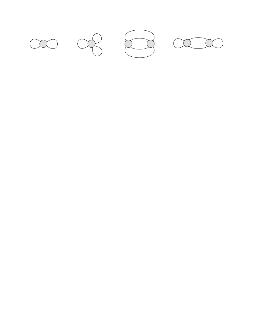
Their contribution to the difference free energy (34) is given by

$$\Delta F_{\mathsf{SA}}{} =\frac{1}{2}\log\det(1-\mathsf{Q}^{-}C^{-})-\frac{1}{8}X_{ij}^{-}X_{kl}^{-}\,\mathsf{Q}_{ijkl}^{-}-\frac{1}{48}X_{ij}^{-}X_{kl}^{-}X_{nm}^{-}\,\mathsf{Q}_{ijklnm}^{-}$$

$$-\frac{1}{48}X_{i_{1}i_{2}}^{-}X_{j_{1}j_{2}}^{-}X_{k_{1}k_{2}}^{-}X_{l_{1}l_{2}}^{-}\mathsf{Q}_{i_{1}j_{1}k_{1}l_{1}}^{-}\mathsf{Q}_{i_{2}j_{2}k_{2}l_{2}}^{-}$$

$$-\frac{1}{16}X_{i_{1}j_{1}}^{-}X_{i_{2}j_{2}}^{-}X_{k_{1}k_{2}}^{-}X_{l_{1}l_{2}}^{-}\mathsf{Q}_{i_{1}j_{1}k_{1}l_{1}}^{-}\mathsf{Q}_{i_{2}j_{2}k_{2}l_{2}}^{-}+O(1/N^{6})\,.$$ (46)

Notice that the semi-infinite matrices $X^{-}$ and $\mathsf{Q}^{-}$ have an expansion in powers of $1/N^{2}$ and, therefore, each term in (2.4) generates a series in $1/N^{2}$.

In the $\mathsf{Q}_{2}$ model, the coefficient in front of the quadratic term in the exponent of (2.3) is two times bigger as compared with that in (41). To use the same propagator as in (45) it is convenient to rescale auxiliary fields in (35) as $J^{-}_{i}\to J^{-}_{i}/\sqrt{2}$ and $J^{+}_{i}\to J^{+}_{i}/\sqrt{2}$. Then, the propagator of $J_{+}$ is defined similar to (45)

$$X_{ij}^{+}\equiv\big{\langle}J_{i}^{+}J_{j}^{+}\big{\rangle}=\left[C^{+}(1-\mathsf{Q}^{+}C^{+})^{-1}\right]_{ij}\,.$$ (47)

The resulting expression for the difference free energy in the $\mathsf{Q}_{2}$ model (35) is

$$\Delta F_{\mathsf{Q}_{2}}{} =\frac{1}{2}\log\det(1-\mathsf{Q}^{-}C^{-})+\frac{1}{2}\log\det(1-\mathsf{Q}^{+}C^{+})$$

$$-\frac{1}{16}X_{ij}^{+}X^{+}_{kl}\mathsf{Q}_{ijkl}^{+}-\frac{1}{16}X_{ij}^{-}X^{-}_{kl}\mathsf{Q}_{ijkl}^{-}-\frac{1}{8}X_{ij}^{+}X^{-}_{kl}\mathsf{Q}_{ijkl}^{+-}+O(1/N^{4})\,.$$ (48)

The first four terms in this relation are analogous to those in (2.4). The last term proportional to $\mathsf{Q}_{ijkl}^{+-}$ takes into account the interaction of $J^{+}$ and $J^{-}$ fields.

In the next section, we first evaluate the individual terms in (2.4) and (2.4) and, then, compute the difference free energy (3) in the two models.

3 Large $N$ expansion of the free energy

The relations (2.4) and (2.4) express the difference free energy in the $\mathsf{SA}$ and $\mathsf{Q}_{2}$ models in terms of two sets of semi-infinite matrices $\mathsf{Q}^{\pm}$ and $C^{\pm}$ defined in (42), (2.3) and (2), respectively. The former are given by correlators in a Gaussian matrix model that are independent of the coupling constant. The latter are fixed by the localization to be nontrivial functions of the coupling constant and are independent of $N$.

The relations (2.4) and (2.4) are valid for any coupling constant. It follows from (2) that $C_{ij}^{\pm}=O(\lambda^{i+j+1})$ at weak coupling and, therefore, the matrices $C^{\pm}$ can be replaced in (2.4) and (2.4) by their finite dimensional minors. Expanding (2.4) and (2.4) in powers of $C^{\pm}$ one can reproduce the weak coupling expansion (2.1) and (2.1).

At strong coupling, we have to find an efficient way to deal with the product of semi-infinite matrices in (2.4) and (2.4). It proves convenient to think about semi-infinite matrices $C^{\pm}$ and $X^{\pm}$ as matrix elements of certain integral operators. In this way, the product of these matrices can be cast into a convolution of the corresponding integral kernels. We show in this section that the integral operators defined by $C^{\pm}$ and $X^{\pm}$ coincide with the temperature dependent (or truncated) Bessel operator. We exploit this property in Section 4 to work out the strong coupling expansion of the difference free energy (2.4) and (2.4).

3.1 Leading order

At large $N$, the leading contribution to (2.4) and (2.4) comes from terms involving $\log\det(1-\mathsf{Q}^{\pm}C^{\pm})$. The contribution of the remaining terms is suppressed by powers of $1/N^{2}$ in virtue of (42), (2.3) and (40).

Let us first summarize the properties of the matrices $\mathsf{Q}_{ij}^{\pm}$ that enter the leading term in (2.4) and (2.4). According to (42) and (2.3), they are given by two-point correlators in a Gaussian matrix model

$$\mathsf{Q}^{-}_{ij}=\big{\langle}\mathcal{O}_{2i+1}\mathcal{O}_{2j+1}\big{\rangle}\,,\qquad\qquad\mathsf{Q}^{+}_{ij}=\big{\langle}\mathcal{O}_{2i}\mathcal{O}_{2j}\big{\rangle}-\big{\langle}\mathcal{O}_{2i}\big{\rangle}\big{\langle}\mathcal{O}_{2j}\big{\rangle}\,.$$ (49)

To the first few orders in $1/N^{2}$ they take the following form

$$\mathsf{Q}^{-}_{ij} =\beta_{i}^{-}\beta_{j}^{-}\left[{2\over i+j+1}+\frac{1}{6N^{2}}(i^{2}+ij+j^{2}-5(i+j)-13)+O(1/N^{4})\right]\,,$$

$$\mathsf{Q}^{+}_{ij} =\beta_{i}^{+}\beta_{j}^{+}\left[{2\over i+j}+\frac{1}{6N^{2}}(i^{2}+ij+j^{2}-8(i+j)+7)+O(1/N^{4})\right]\,,$$ (50)

where normalization factors are

$$\beta_{i}^{+}=2^{1/2-i}{\Gamma(2i)\over\Gamma^{2}(i)}\,,\qquad\qquad\beta_{i}^{-}=2^{-1-i}{\Gamma(2i+2)\over\Gamma(i+2)\Gamma(i)}\,.$$ (51)

These relations match (40) for $L=2$.

The leading $O(N^{0})$ term in (3.1) admits the following representation

$$\mathsf{Q}^{\pm}=U^{\pm}(U^{\pm})^{t}+O(1/N^{2})\,,$$ (52)

where $U^{\pm}$ are lower triangular matrices and $(U^{\pm})^{t}$ denote transposed matrices. The explicit expression for these matrices can be found in (B).  We apply the matrices $U^{\pm}$ to define

$$K^{\pm}=(U^{\pm})^{t}C^{\pm}U^{\pm}\,.$$ (53)

A distinguished feature of these matrices is that they admit an integral representation in terms of Bessel functions, see (77) and (75) below. Combining together (52) and (53) we obtain

$$\log\det(1-\mathsf{Q}^{\pm}C^{\pm})=\log\det(1-K^{\pm})+O(1/N^{2})\,.$$ (54)

As we will see in a moment, the expression on the right-hand side coincides with a Fredholm determinant of the Bessel operator.

To summarize, the leading corrections to the difference free energy (2.4) and (2.4) in the $\mathsf{SA}$ and $\mathsf{Q}_{2}$ models are given by

$$\mathsf{F}_{0}^{\mathsf{SA}}=\frac{1}{2}\log\det(1-K^{-})\,,$$

$$\mathsf{F}_{0}^{\mathsf{Q}_{2}}=\frac{1}{2}\log\det(1-K^{-})+\frac{1}{2}\log\det(1-K^{+})\,.$$ (55)

3.2 Subleading corrections

To compute subleading corrections to (54) in $1/N^{2}$, we generalize (52) as

$$\mathsf{Q}^{\pm}=U^{\pm}\mathsf{R}^{\pm}(U^{\pm})^{t}\,,$$ (56)

where $\mathsf{R}^{\pm}=1+O(1/N^{2})$. To determine the (matrix) coefficients in the expansion of $\mathsf{R}^{\pm}$ in powers of $1/N^{2}$, we apply an inverse transformation to the matrices (3.1).

To any order in $1/N^{2}$, the correlators (3.1) are given by a sum of terms of the form $\beta_{i}\beta_{j}i^{n}j^{m}$

$$\mathsf{Q}^{\pm}=U^{\pm}(U^{\pm})^{t}+{1\over N^{2}}\beta_{i}\beta_{j}\sum_{n,m\geq 0}c_{nm}^{\pm}i^{n}j^{m}\,,$$ (57)

where the expansion coefficients $c_{nm}^{\pm}$ are series in $1/N^{2}$ with rational coefficients. They can be found by matching (57) to the expression (3.1) of the two-point correlators $\mathsf{Q}^{\pm}$. For instance, for $N\to\infty$ the only nonzero entries are

$$c_{02}^{\pm}=c_{11}^{\pm}=\tfrac{1}{6}\,,\qquad c_{01}^{+}=-\tfrac{4}{3}\,,\qquad c_{01}^{-}=-\tfrac{5}{6}\,,\qquad c_{00}^{+}=\tfrac{7}{6}\,,\qquad c_{00}^{-}=-\tfrac{13}{6}\,.$$ (58)

and $c_{nm}^{\pm}=c_{mn}^{\pm}$.

Combining together (56) and (57), we find

$$\mathsf{R}^{\pm}=1+{1\over N^{2}}\sum_{n,m}c_{nm}^{\pm}R_{nm}^{\pm}\,.$$ (59)

As compared to (57), each term of the sum gets replaced by a matrix $R_{n,m}=R_{n}\otimes R_{m}$ defined as

$$(R_{nm})_{ij}=(R_{n})_{i}(R_{m})_{j}\,,\qquad\qquad(R_{n})_{i}=\sum_{k\geq 1}U_{ik}^{-1}k^{n}\beta_{k}\,.$$ (60)

To simplify the formula, we do not display here the superscript ‘$\pm$’. The explicit expressions for the vectors $R_{n}^{\pm}$ can be found in Appendix B.

It follows from (59) and (58) that the semi-infinite matrices $\mathsf{R}^{\pm}$ are given to order $O(1/N^{2})$ by

$$\mathsf{R}^{+}=1+{1\over 6N^{2}}\left[R_{0,2}^{+}+R_{2,0}^{+}+R_{1,1}^{+}-8R_{1,0}^{+}-8R_{0,1}^{+}+7R_{0,0}^{+}\right]+O(1/N^{4})\,,$$

$$\mathsf{R}^{-}=1+{1\over 6N^{2}}\left[R_{0,2}^{-}+R_{2,0}^{-}+R_{1,1}^{-}-5R_{1,0}^{-}-5R_{0,1}^{-}-13R_{0,0}^{-}\right]+O(1/N^{4})\,.$$ (61)

The main advantage of dealing with matrices $\mathsf{R}^{\pm}$ is that they allow us to express the subleading corrections to the free energy (2.4) and (2.4) in terms of the same matrices $K^{\pm}$ that appeared at the leading order (3.1).

To show this we take into account (53), (56) and (59) to obtain

$$\log\det(1-\mathsf{Q}^{\pm}C^{\pm}) =\log\det(1-\mathsf{R}^{\pm}K^{\pm})$$

$$=\log\det(1-K^{\pm})+\log\det\Big{(}1-{1\over N^{2}}\sum_{n,m}c^{\pm}_{nm}R_{n,m}^{\pm}{K^{\pm}\over 1-K^{\pm}}\Big{)}\,.$$ (62)

Expanding the second term on the right-hand side in powers of $R^{\pm}$ and using a factorized form of this matrix, $R_{nm}=R_{n}\otimes R_{m}$, we get

$$\log\det(1-\mathsf{Q}^{\pm}C^{\pm})=\log\det(1-K^{\pm})-\sum_{L\geq 1}{1\over LN^{2L}}c^{\pm}_{n_{1},m_{1}}W^{\pm}_{m_{1},n_{2}}c^{\pm}_{n_{2},m_{2}}\dots c^{\pm}_{n_{L},m_{L}}W^{\pm}_{m_{L},n_{1}}\,,$$ (63)

where the notation was introduced for the scalar quantity

$$W^{\pm}_{nm}=(R^{\pm}_{n}{)}_{i}{\left({K^{\pm}\over 1-K^{\pm}}\right)}_{ij}(R^{\pm}_{m}{)}_{j}\,,\qquad\qquad(n,m\geq 0)\,.$$ (64)

It is symmetric in indices, $W^{\pm}_{nm}=W^{\pm}_{mn}$, depends on the ’t Hooft coupling $\lambda$ but is independent of $N$. Expansion of $W^{\pm}_{nm}$ at strong coupling is derived in Section 4.

The relation (63) can be used to systematically expand $\log\det(1-\mathsf{Q}^{\pm}C^{\pm})$ in powers of $1/N^{2}$. In particular, the $O(1/N^{2})$ correction to (63) is given by

$$\frac{1}{2}\log\det(1-\mathsf{Q}^{+}C^{+})\Big{|}_{O(1/N^{2})}=-\frac{7}{12}W^{+}_{0,0}+\frac{4}{3}W^{+}_{0,1}-\frac{1}{6}W^{+}_{0,2}-\frac{1}{12}W^{+}_{1,1}\,,$$

$$\frac{1}{2}\log\det(1-\mathsf{Q}^{-}C^{-})\Big{|}_{O(1/N^{2})}=\frac{13}{12}W^{-}_{0,0}+\frac{5}{6}W^{-}_{0,1}-\frac{1}{6}W^{-}_{0,2}-\frac{1}{12}W^{-}_{1,1}\,.$$ (65)

Let us now examine the remaining terms in (2.4) and (2.4). They contain the product of matrices $X^{\pm}$ whose indices are contracted with the $\mathsf{Q}-$tensors, e.g. $X_{ij}^{-}X^{-}_{kl}\mathsf{Q}_{ijkl}^{-}$ and $X_{ij}^{+}X^{-}_{kl}\mathsf{Q}_{ijkl}^{+-}$. Applying (53) and (56), we can express the matrices $X^{\pm}$ defined in (45) and (47), in terms of the Bessel matrices (78)

$$X^{\pm}=(U^{\pm\,t})^{-1}K^{\pm}(1-\mathsf{R}^{\pm}K^{\pm})^{-1}(U^{\pm})^{-1}\,.$$ (66)

According to (40), (42) and (2.3), the $\mathsf{Q}-$tensors are proportional to the product of $\beta-$factors and certain polynomials in indices. As a result, $X_{ij}^{-}X^{-}_{kl}\mathsf{Q}_{ijkl}^{-}$ and $X_{ij}^{+}X^{-}_{kl}\mathsf{Q}_{ijkl}^{+-}$ are given by a sum of terms each of which factorizes into a product of terms of the form

$$i^{n}j^{m}\beta_{i}^{\pm}\beta_{j}^{\pm}X^{\pm}_{ij}{} =(R_{n})_{i}(K^{\pm}(1-\mathsf{R}^{\pm}K^{\pm})^{-1})_{ij}(R_{m})_{j}$$

$$=W^{\pm}_{nm}+\sum_{L\geq 1}{1\over N^{2L}}W^{\pm}_{nn_{1}}c^{\pm}_{n_{1}m_{1}}W^{\pm}_{m_{1}n_{2}}\dots c^{\pm}_{n_{L}m_{L}}W^{\pm}_{m_{L}m}\,.$$ (67)

Here in the first relation we took into account (60) and in the second relation expanded the right-hand side in powers of $\mathsf{R}^{\pm}$ and applied (59) and (64).

The relation (3.2) allows us to express various terms in (2.4) and (2.4) in terms of the matrix elements (64). As an example, the leading $O(1/N^{2})$ correction to the second term in (2.4) can be computed as

$$-\frac{1}{8}X_{ij}^{-}X_{kl}^{-}\,\mathsf{Q}_{ijkl}^{-}{} =-(2+i+j)\beta_{i}^{-}\beta_{j}^{-}X^{-}_{ij}\beta_{k}^{-}\beta_{l}^{-}X^{-}_{kl}+O(1/N^{4})$$

$$=-2(W_{0,0}^{-}+W^{-}_{0,1})W^{-}_{0,0}+O(1/N^{4})\,,$$ (68)

where we replaced $\mathsf{Q}_{ijkl}^{-}$ with its expression (A) and applied (3.2).

Combining together the above relations we obtain from (2.4) and (2.4) the $O(1/N^{2})$ correction to the difference free energy (3) in the $\mathsf{SA}$ and $\mathsf{Q}_{2}$ models

$$\mathsf{F}_{1}^{\mathsf{SA}}={} -2W_{0,0}^{-}(W_{0,0}^{-}+W^{-}_{0,1})+\frac{13}{12}W^{-}_{0,0}+\frac{5}{6}W^{-}_{0,1}-\frac{1}{6}W^{-}_{0,2}-\frac{1}{12}W^{-}_{1,1}\,,$$

$$\mathsf{F}_{1}^{\mathsf{Q}_{2}}={} -(W^{+}_{0,0}+W^{-}_{0,0})(W^{+}_{0,1}+W^{-}_{0,1})-(W^{-}_{0,0})^{2}+\frac{1}{4}(W^{+}_{0,0})^{2}$$

$$+\frac{13}{12}W^{-}_{0,0}+\frac{5}{6}W^{-}_{0,1}-\frac{1}{6}W^{-}_{0,2}-\frac{1}{12}W^{-}_{1,1}-\frac{7}{12}W^{+}_{0,0}+\frac{4}{3}W^{+}_{0,1}-\frac{1}{6}W^{+}_{0,2}-\frac{1}{12}W^{+}_{1,1}\,.$$ (69)

Notice that the expression for $\mathsf{F}_{1}^{\mathsf{Q}_{2}}$ contains mixed terms proportional to the product of $W^{+}$ and $W^{-}$. They come from $X_{ij}^{+}X^{-}_{kl}\mathsf{Q}_{ijkl}^{+-}$ term in (2.4).

The same technique can be used to determine subleading $O(1/N^{4})$ correction to the free energy (3). Going through the calculation we obtain in the $\mathsf{SA}$ model

$$\mathsf{F}_{2}^{\mathsf{SA}} =-\frac{64}{3}W_{0,0}^{4}-\frac{128}{3}W_{0,1}W_{0,0}^{3}-\frac{10}{3}W_{1,1}W_{0,0}^{3}-18W_{0,1}^{2}W_{0,0}^{2}+\frac{11}{3}W_{0,0}^{3}-\frac{86}{3}W_{0,1}W_{0,0}^{2}-\frac{49}{3}W_{0,2}W_{0,0}^{2}$$

$$-W_{0,3}W_{0,0}^{2}-\frac{31}{3}W_{1,1}W_{0,0}^{2}-\frac{10}{3}W_{1,2}W_{0,0}^{2}-\frac{131}{3}W_{0,1}^{2}W_{0,0}-13W_{0,1}W_{0,2}W_{0,0}-\frac{37}{3}W_{0,1}W_{1,1}W_{0,0}$$

$$-\frac{25}{3}W_{0,1}^{3}-\frac{133}{144}W_{0,0}^{2}+\frac{499}{36}W_{0,1}W_{0,0}+\frac{307}{36}W_{0,2}W_{0,0}-\frac{1}{6}W_{0,3}W_{0,0}-\frac{1}{6}W_{0,4}W_{0,0}+\frac{443}{72}W_{1,1}W_{0,0}$$

$$+\frac{41}{36}W_{1,2}W_{0,0}-\frac{1}{2}W_{1,3}W_{0,0}-\frac{25}{72}W_{2,2}W_{0,0}+\frac{77}{6}W_{0,1}^{2}-\frac{49}{72}W_{0,2}^{2}-\frac{37}{144}W_{1,1}^{2}+\frac{77}{36}W_{0,1}W_{0,2}$$

$$-W_{0,1}W_{0,3}+\frac{131}{36}W_{0,1}W_{1,1}-W_{0,2}W_{1,1}-\frac{73}{36}W_{0,1}W_{1,2}+\frac{37}{60}W_{0,0}+\frac{41}{180}W_{0,1}-\frac{151}{120}W_{0,2}-\frac{31}{240}W_{0,3}$$

$$+\frac{1}{10}W_{0,4}-\frac{1}{144}W_{0,5}-\frac{151}{240}W_{1,1}-\frac{251}{360}W_{1,2}+\frac{71}{240}W_{1,3}-\frac{1}{48}W_{1,4}+\frac{5}{24}W_{2,2}-\frac{29}{720}W_{2,3}\,,$$

where $W_{n,m}\equiv W_{n,m}^{-}$.

We would like to emphasize that the relations (3.1), (3.2) and (3.2) hold for an arbitrary ’t Hooft coupling. We verified that at weak coupling they are in agreement with (2.1) and (2.1).

3.3 Relation to the Bessel operator

In what follows we shall use the notation

$$g\equiv{\sqrt{\lambda}\over 4\pi}\ .$$ (71)

Let us show that the semi-infinite matrices (53) are given by matrix elements of the truncated Bessel operator $\bm{K}_{\ell}$. This operator is defined as

$$\bm{K}_{\ell}f(x) =\int_{0}^{\infty}dy\,K_{\ell}(x,y)\chi{\left({\sqrt{y}\over 2g}\right)}f(y)\,,$$ (72)

where $f(x)$ is a test function and $K_{\ell}(x,y)$ is expressed in terms of the Bessel functions (hence the name of the operator)

$$K_{\ell}(x,y) =\sum_{i\geq 1}\psi_{i}(x)\psi_{i}(y)={\sqrt{x}J_{\ell+1}(\sqrt{x})J_{\ell}(\sqrt{y})-\sqrt{y}J_{\ell+1}(\sqrt{y})J_{\ell}(\sqrt{x})\over 2(x-y)}\,.$$ (73)

Here $\ell$ is an arbitrary positive real parameter and $\psi_{i}(x)$ is an orthonormal basis of functions

$$\psi_{i}(x)=(-1)^{i}\sqrt{2i+\ell-1}{J_{2i+\ell-1}(\sqrt{x})\over\sqrt{x}}\,,$$

$$\big{\langle}\psi_{i}|\psi_{j}\big{\rangle}=\int_{0}^{\infty}dx\,\psi_{i}(x)\psi_{j}(x)=\delta_{ij}\,.$$ (74)

The function $\chi(x)$ is conventionally called the “symbol” of the Bessel operator. In what follows we choose this function as

$$\chi(x)=-{1\over\sinh^{2}(x/2)}\,.$$ (75)

It vanishes at infinity and truncates the integral in (72) at $y=O(g^{2})$.

The Bessel operator (72) can be realized as a semi-infinite matrix on the space of functions spanned by $\psi_{i}(x)$

$$\bm{K}_{\ell}\,\psi_{i}(x)=(K_{\ell})_{ij}\psi_{j}(x)\,.$$ (76)

Its matrix elements $(K_{\ell})_{ij}=\big{\langle}\psi_{i}|\bm{K}_{\ell}|\psi_{j}\big{\rangle}$ are given by

$$(K_{\ell})_{ij}=(-1)^{i+j}\sqrt{2i+\ell-1}\sqrt{2j+\ell-1}\,\int_{0}^{\infty}\frac{dt}{t}\,J_{2i+\ell-1}(\sqrt{t})\,J_{2j+\ell-1}(\sqrt{t})\chi{\left({\sqrt{t}\over 2g}\right)}\,.$$ (77)

where $i,j\geq 1$.

The reason for the choice of the symbol function (75) is that the resulting matrix $K_{\ell}$ coincides for $\ell=1$ and $\ell=2$ with the semi-infinite matrices $K^{\pm}$ defining the leading contribution to the free energy (3.1) ,

$$K^{+}=K_{\ell=1}\,,\qquad\qquad K^{-}=K_{\ell=2}\,.$$ (78)

Being combined with (3.1), this relation implies that the $O(N^{0})$ contribution to the difference free energy in $\mathsf{SA}$ and $\mathsf{Q}_{2}$ models is given by a Fredholm determinant of the Bessel operator

$$\mathsf{F}_{0}^{\mathsf{SA}}=\frac{1}{2}\log\det(1-\bm{K}_{\ell=2})\,,$$

$$\mathsf{F}_{0}^{\mathsf{Q}_{2}}=\frac{1}{2}\log\det(1-\bm{K}_{\ell=1})+\frac{1}{2}\log\det(1-\bm{K}_{\ell=2})\,.$$ (79)

For the special choice of the symbol $\chi(x)=\theta(1-x)$, the Fredholm determinant of the Bessel operator coincides with the celebrated Tracy-Widom distribution describing statistics of the spacing of the eigenvalues in Laguerre ensemble Tracy:1993xj . In application to the $\mathsf{SA}$ and $\mathsf{Q}_{2}$ models, we encounter the symbol of the form (75).

Strong coupling expansion of (3.3) was derived in Beccaria:2022ypy using the technique developed in Belitsky:2019fan ; Belitsky:2020qrm ; Belitsky:2020qir . It relies on the relation

$$\log{} \det(1-\bm{K}_{\ell})=\pi g-\frac{1}{2}{\left({2\ell-1}\right)}\log g+B_{\ell}+\frac{1}{8}(2\ell-3)(2\ell-1)\log(g^{\prime}/g)$$ (80)

$$+(2\ell-5)(2\ell-3)(4\ell^{2}-1){\zeta(3)\over 2048\pi^{3}g^{\prime}{}^{3}}-(2\ell-7)(2\ell-5)(4\ell^{2}-9)(4\ell^{2}-1){3\zeta(5)\over 262144\pi^{5}g^{\prime}{}^{5}}+\dots\ .$$

Here $g$ is defined in (71),   $g^{\prime}=g-{\log 2/\pi}$ and dots denote subleading corrections suppressed by powers of $1/g$ as well as exponentially small $O(e^{-4\pi g})$ corrections. Expanding again the series in powers of $1/g$, one can produce terms proportional to powers of $\log 2/\pi$. The constant term $B_{\ell}$ in (80), conventionally called the Widom-Dyson constant, is given by

$$B_{\ell}=-6\log\mathsf{A}+\frac{1}{2}+\frac{1}{6}\log 2-\ell\log 2+\log\Gamma(\ell)\,,$$ (81)

where $\mathsf{A}$ is the Glaisher’s constant. Substituting (80) into (3.3) we arrive at

$$\mathsf{F}_{0}^{\mathsf{SA}}=\frac{\pi g}{2}-\frac{3\log g}{4}-3\log\mathsf{A}+\frac{1}{4}-\frac{11\log 2\,}{12}+\frac{3}{16}\log\frac{g^{\prime}}{g}-\frac{15\zeta(3)}{4096(\pi g^{\prime})^{3}}-\frac{945\zeta(5)}{524288(\pi g^{\prime})^{5}}+\dots\,,$$

$$\mathsf{F}_{0}^{\mathsf{Q}_{2}}=\pi g-\log g-6\log\mathsf{A}+\frac{1}{2}-\frac{4\log 2\,}{3}+\frac{1}{8}\log\frac{g^{\prime}}{g}-\frac{3\zeta(3)}{2048(\pi g^{\prime})^{3}}-\frac{135\zeta(5)}{262144(\pi g^{\prime})^{5}}+\dots\,,$$ (82)

where $g^{\prime}$ is defined in (80). For $g={\sqrt{\lambda}/4\pi}$ these relations coincide with (4) and (5).

Subleading corrections to the free energy (3.2) and (3.2) involve the quantities $W_{nm}^{\pm}$ defined in (64). To establish the relation between $W_{nm}^{\pm}$ and the Bessel operator, it is convenient to introduce auxiliary functions $\phi_{n}^{\pm}(x)$ with $n\geq 0$

$$\phi_{n}^{\pm}(x)=\sum_{i\geq 1}(R^{\pm}_{n}{)}_{i}\,\psi_{i}^{\pm}(x)\,,$$ (83)

where $\psi_{i}^{+}(x)$ and $\psi_{i}^{-}(x)$ coincide with (3.3) for $\ell=1$ and $\ell=2$, respectively, and the expansion coefficients $(R^{\pm}_{n}{)}_{i}$ are defined in (60). The matrices (78) and (77) admit the representation

$$K^{\pm}_{ij}=\int_{0}^{\infty}dt\,\psi_{i}^{\pm}(t)\chi{\left({\sqrt{t}\over 2g}\right)}\psi_{j}^{\pm}(t)\,.$$ (84)

Their product can be expressed using (73) as a convolution of the Bessel kernels

$$[(K^{\pm})^{L}]_{ij}=\int_{0}^{\infty}{} dt_{1}\dots dt_{L}\,\psi_{i}^{\pm}(t_{1})\chi{\left({\sqrt{t}_{1}\over 2g}\right)}$$

$$\times K^{\pm}(t_{1},t_{2})\chi{\left({\sqrt{t}_{2}\over 2g}\right)}\dots K^{\pm}(t_{L},t_{L-1})\chi{\left({\sqrt{t}_{L}\over 2g}\right)}\psi_{j}^{\pm}(t_{L})\,,$$ (85)

where $K^{\pm}(x,y)$ is the kernel (73) evaluated at $\ell=1$ and $\ell=2$. This relation can be written in a compact form as

$$[(K^{\pm})^{L}]_{ij}=\big{\langle}\psi_{i}^{\pm}|\bm{\chi}\,(\bm{K}^{\pm})^{L-1}|\psi_{j}^{\pm}\big{\rangle}\ ,$$ (86)

where the operator $\bm{\chi}$ has a diagonal kernel $\delta(x-y)\chi(\sqrt{x}/(2g))$.

We apply the relation (86) to obtain the following representation of (64)

$$W^{\pm}_{nm}{} =(R^{\pm}_{n}{)}_{i}\big{\langle}\psi_{i}^{\pm}|\bm{\chi}\,{1\over 1-\bm{K}^{\pm}}|\psi_{j}^{\pm}\big{\rangle}(R^{\pm}_{m}{)}_{j}=\big{\langle}\phi_{n}^{\pm}|\bm{\chi}{1\over 1-\bm{K}^{\pm}}|\phi_{m}^{\pm}\big{\rangle}\,,$$ (87)

where in the second relation we used (83). Thus, the quantities $W_{nm}^{\pm}$ are given by matrix elements of the resolvent of the Bessel operator with respect to the special states $\phi_{n}^{\pm}(x)$ defined in (83).

According to (83), the functions $\phi_{n}^{\pm}(x)$ are given by infinite sums of the Bessel functions (3.3) with the expansion coefficients (60). These sums can evaluated in a closed form leading to (see Appendix B)

$$\phi_{n}^{-}(x)=-\frac{1}{2\sqrt{2}}(x\partial_{x})^{n}J_{2}(\sqrt{x})\,,$$

$$\phi_{n}^{+}(x)=-\frac{1}{2\sqrt{2}}\sum_{i=0}^{n}2^{i-n}{\left({n\atop i}\right)}(x\partial_{x})^{i}J_{1}(\sqrt{x})\,.$$ (88)

To summarize, we demonstrated in this section that non-planar corrections to the free energy admit a compact representation (3.2) and (3.2) in terms of the matrix elements $W^{\pm}_{nm}$ of the resolvent (87) of the truncated Bessel operator. In the next section, we develop a technique for computing $W^{\pm}_{nm}$ and, then, apply it to derive the strong coupling expansion of the free energy (3.2) and (3.2).

4 Resolvent of the Bessel operator

The matrix elements (87) involve the Bessel operator (72) for $\ell=1$ and $\ell=2$ (see (78)). To treat them in a unified manner, we generalize (87) to arbitrary $\ell$ and define the matrix elements of the resolvent of the Bessel operator (72)

$$w_{nm}=\big{\langle}\phi_{n}|\bm{\chi}{1\over 1-\bm{K}_{\ell}}|\phi_{m}\big{\rangle}\,,$$ (89)

where the functions $\phi_{n}(x)$ (with $n\geq 0$) are given by

$$\phi_{0}(x)=J_{\ell}(\sqrt{x})\,,\qquad\qquad\phi_{n}(x)=(x\partial_{x})^{n}\phi_{0}(x)\,.$$ (90)

The operator $\bm{\chi}$ is defined in (86), it acts on a test function as $\bm{\chi}f(x)=\chi(\sqrt{x}/(2g))f(x)$.

In the previous section, we encountered different matrix elements (87). As follows from (87) and (3.3), they are given by a linear combination of $w_{nm}$ evaluated for $\ell=1$ and $\ell=2$

$$W_{nm}^{-}=\frac{1}{8}w_{nm}\Big{|}_{\ell=2}\,,$$

$$W_{nm}^{+}=\frac{1}{8}\sum_{i=0}^{n}\sum_{j=0}^{m}2^{i+j-n-m}{\left({n\atop i}\right)}{\left({m\atop j}\right)}w_{ij}\Big{|}_{\ell=1}\,.$$ (91)

The matrix elements (89) depend on the integer $\ell$ and the coupling constant $g=\sqrt{\lambda}/(4\pi)$. They have the following important properties. Expanding (89) in powers of $\bm{K}_{\ell}$ and taking into account the definition (72) of the Bessel operator, we find that $w_{nm}$ are symmetric in indices

$$w_{mn}=w_{nm}\,.$$ (92)

Besides, the matrix elements (89) are not independent. We show in Appendix C that $w_{nm}$ satisfy a functional equation

$${\left({\frac{1}{2}g\partial_{g}-1}\right)}w_{nm}=\frac{1}{4}w_{0n}w_{0m}+w_{n+1,m}+w_{n,m+1}\,.$$ (93)

For lowest values of $n,m\geq 0$ it leads to

$$w_{01}{} =-\frac{1}{8}w_{00}^{2}+{\left({\frac{1}{4}g\partial_{g}-\frac{1}{2}}\right)}w_{00}\,,$$

$$w_{11}{} =-w_{02}-\frac{1}{4}w_{01}w_{00}+{\left({\frac{1}{2}g\partial_{g}-1}\right)}w_{01}\,,$$

$$w_{12}{} =-\frac{1}{8}w_{01}^{2}+{\left({\frac{1}{4}g\partial_{g}-\frac{1}{2}}\right)}w_{11}\,,\qquad\dots\,.$$ (94)

These relations hold for an arbitrary coupling. They allow us to express $w_{01}$, $w_{11}$ and $w_{12}$ in terms of $w_{00}$ and $w_{02}$. Examining the relation (93) for arbitrary $m$ and $n$, we find that the matrix elements $w_{nm}$ can be expressed in terms of independent quantities $w_{00},w_{02},w_{04},\dots$. We discuss them in the next subsection.

4.1 Method of differential equations

The matrix element $w_{00}$ is related to the Fredholm determinant of the Bessel operator (see Belitsky:2019fan ; Belitsky:2020qrm ; Belitsky:2020qir )

$$w_{00}=-2g\partial_{g}\log\det(1-\bm{K}_{\ell})\,.$$ (95)

Its expansion at strong coupling follows from (80)

$$w_{00}={} -2\pi g+(2\ell-1)-\frac{(2\ell-3)(2\ell-1)\log 2}{4\pi g}-\frac{(2\ell-3)(2\ell-1)\log^{2}2}{4(\pi g)^{2}}$$

$$+\frac{(2\ell-3)(2\ell-1)\left(3\zeta(3)(2\ell-5)(2\ell+1)-256\log^{3}2\right)}{1024(\pi g)^{3}}+\dots\,,$$ (96)

where $g=\sqrt{\lambda}/(4\pi)$. Substituting this expression into the first relation in (4), we can obtain the strong coupling expansion of $w_{01}$.

The strong coupling expansion of $w_{0n}$ can be found by applying the method of differential equations Korepin:1993kvr ; Tracy:1993xj . It is based on the following identify Belitsky:2019fan (see (C) in Appendix C)

$$\partial_{g}w_{0n}{} =\int_{0}^{\infty}dx\,Q_{0}(x)Q_{n}(x)\partial_{g}\chi{\left({\sqrt{x}\over 2g}\right)}\,,$$ (97)

where the functions $Q_{n}(x)$ (with $n\geq 0$) are matrix elements of the resolvent of the Bessel operator

$$Q_{n}(x)=\big{\langle}x|{1\over 1-\bm{K}_{\ell}}|\phi_{n}\big{\rangle}\,.$$ (98)

It is tacitly assumed that $Q_{n}(x)$ also depends on the coupling $g$.

We show in Appendix C that the functions $Q_{n}(x)$ satisfy recurrence relations

$$Q_{n+1}(x)=-\frac{1}{4}Q_{0}(x)w_{0n}(g)+\frac{1}{2}{\left({g\partial_{g}+2x\partial_{x}}\right)}Q_{n}(x)\,.$$ (99)

They can be used to express $Q_{n}(x)$ for $n\geq 1$ in terms of $Q_{0}(x)$. In its turn, the function $Q_{0}(x)$ satisfies a second-order partial differential equation Belitsky:2020qrm ; Belitsky:2020qir

$$\Big{[}(g\partial_{g}+2x\partial_{x})^{2}+x-\ell^{2}+(1-g\partial_{g})w_{00}\Big{]}Q_{0}(x)=0\,.$$ (100)

It involves a nontrivial function of the coupling $w_{00}$ given by (95) and (4.1). A solution to the differential equation (100) at strong coupling is described in Appendix C. Being combined with (99), it allows us to expand the integral on the right-hand side of (97) in powers of $1/g$ and, then, obtain the strong coupling expansion of $w_{0n}$.

In this way we obtain

$$w_{02}{} =\frac{(\pi g)^{3}}{4}+\frac{1}{8}(\pi g)^{2}(2\ell-1)+\pi g\left(-\frac{\ell^{2}}{2}-\frac{1}{32}(2\ell-3)(2\ell-1)\log 2\right)$$

$$+\left(\frac{1}{32}(2\ell-1)\left(4\ell^{2}+4\ell+3\right)+\frac{1}{32}(2\ell-3)(2\ell-1)\log 2\,(2\ell+1-\log 2\,)\right)+O(1/g)\,,$$

$$w_{04}{} =-\frac{23(\pi g)^{5}}{64}-\frac{5(\pi g)^{4}}{128}(2\ell-9)+{(\pi g)^{3}\over 8}\left(\left(\ell^{2}-2\ell+2\right)+\frac{5}{64}(2\ell-3)(2\ell-1)\log 2\right)$$

$$+{(\pi g)^{2}\over 256}\left(\left(12\ell^{2}-12\ell+11\right)(2\ell-1)-\frac{1}{2}(2\ell-3)(2\ell-1)(2(2\ell-7)\log 2-5\log^{2}2)\right)+O(g)\,.$$ (101)

We recall that all other matrix elements $w_{nm}$ follow unambiguously from the functional relations (93).

Examining the relations (4.1) and (4.1), we observe that the matrix elements $w_{0n}$ behave at strong coupling as a power of $g$

$$w_{0n}=\omega_{0n}\,g^{n+1}+O(g^{n})\,.$$ (102)

It follows from (93) that $w_{nm}$ have a similar behaviour

$$w_{nm}=\omega_{nm}\,g^{n+m+1}+O(g^{n+m})\,.$$ (103)

The explicit expressions for the leading coefficients $\omega_{nm}$ are given by relations (127) – (129) below. Most importantly they are independent of $\ell$. 

We recall that the free energy in the $\mathsf{SA}$ and $\mathsf{Q}_{2}$ models is expressed in terms of the matrix elements (4) evaluated at $\ell=1$ and $\ell=2$. The fact that the leading asymptotic behaviour of $w_{nm}$ at strong coupling is independent of $\ell$ suggests that the free energy in the two models should be related to each other. Indeed, we establish such a relation in Section 5.1 below.

4.2 Next-to-leading corrections to the free energy

We are now ready to compute the subleading corrections to the (difference) free energy (3.2).

Applying the relations (4) we can express $F_{1}^{\mathsf{SA}}$ and $F_{1}^{\mathsf{Q}_{2}}$ in terms of the matrix elements $w_{nm}$

$$F_{1}^{\mathsf{SA}}={} -{1\over 32}w_{00}^{-}(w_{00}^{-}+w_{01}^{-})+\frac{13}{96}w_{00}^{-}+\frac{5}{48}w_{01}^{-}-\frac{1}{48}w_{02}^{-}-\frac{1}{96}w_{11}^{-}\,,$$

$$F_{1}^{\mathsf{Q}_{2}}={} -\frac{1}{64}(w^{+}_{01}+w^{-}_{01})(w^{+}_{0,0}+w^{-}_{00})-\frac{1}{128}w^{+}_{00}w^{-}_{00}-\frac{1}{64}(w^{-}_{00})^{2}-\frac{1}{256}(w^{+}_{00})^{2}$$

$$+\frac{w^{+}_{00}}{384}+\frac{13}{96}w^{+}_{01}-\frac{1}{48}w^{+}_{02}-\frac{1}{96}w^{+}_{11}+\frac{13}{96}w^{-}_{00}+\frac{5}{48}w^{-}_{01}-\frac{1}{48}w^{-}_{02}-\frac{1}{96}w^{-}_{11}\,,$$ (104)

where $w_{nm}^{+}$ and $w_{nm}^{-}$ are given by $w_{nm}$ for $\ell=1$ and $\ell=2$, respectively.

Replacing the matrix elements with their expressions (4.1), (4.1) and (4), we obtain the strong coupling expansion of the difference free energy in the two models

$$F^{\mathsf{SA}}_{1} =-\frac{(\pi g)^{3}}{32}-\frac{3(\pi g)^{2}}{128}+\pi g\left(\frac{11}{512}-\frac{\log 2\,}{32}\right)+\left(\frac{3}{128}-\frac{\log^{2}2}{32}-\frac{\log 2\,}{512}\right)$$

$$+{\left({-\frac{15\zeta(3)}{8192}-\frac{\log^{3}2}{32}-\frac{3\log^{2}2}{512}+\frac{279\log 2\,}{8192}}\right)}{1\over\pi g}$$

$$+{\left({\frac{105\zeta(3)}{131072}-\frac{15\zeta(3)\log 2\,}{2048}-\frac{\log^{4}2}{32}-\frac{5\log^{3}2}{512}+\frac{441\log^{2}2}{8192}}\right)}{1\over(\pi g)^{2}}+O(1/g^{3})\,,$$ (105)

$$F_{1}^{\mathsf{Q}_{2}} =-\frac{(\pi g)^{3}}{16}-\frac{(\pi g)^{2}}{192}+\pi g\left(\frac{5}{256}-\frac{\log 2\,}{48}\right)+\left(\frac{\log 2\,}{256}-\frac{\log^{2}2}{48}\right)$$

$$+{\left({-\frac{3\zeta(3)}{4096}-\frac{\log^{3}2}{48}+\frac{\log^{2}2}{256}+\frac{35\log 2\,}{4096}}\right)}{1\over\pi g}$$

$$+{\left({\frac{21\zeta(3)}{65536}-\frac{3\zeta(3)\log 2\,}{1024}-\frac{\log^{4}2}{48}+\frac{\log^{3}2}{256}+\frac{53\log^{2}2}{4096}}\right)}{1\over(\pi g)^{2}}+O(1/g^{3})\,.$$ (106)

For $g=\sqrt{\lambda}/(4\pi)$ these relations coincide with (6) and (8).

The following comments are in order.

A close examination of (3.3) shows that the leading $O(N^{0})$ terms of the strong coupling expansion (3) of the free energy in the $\mathsf{SA}$ and $\mathsf{Q}_{2}$ models differ by the factor of $2$. It follows from (4.2) and (4.2) that the same relation holds at order $O(1/N^{2})$

$${F_{0}^{\mathsf{SA}}\over F_{0}^{\mathsf{Q}_{2}}}=\frac{1}{2}+O(1/g)\,,\qquad\qquad{F_{1}^{\mathsf{SA}}\over F_{1}^{\mathsf{Q}_{2}}}=\frac{1}{2}+O(1/g)\,.$$ (107)

This relation is yet another manifestation of universality of matrix elements mentioned in the previous subsection. We show in Section 5.1 that it holds to any order of $1/N^{2}$ expansion (3).

It is important to emphasize that the relations (107) only hold at strong coupling. At weak coupling, one uses (2.1) and (2.1) to verify that the ratios of functions differ already at order $O(g^{2})$

$${F_{0}^{\mathsf{SA}}\over F_{0}^{\mathsf{Q}_{2}}}={10\zeta(5)\over 3\zeta(3)}g^{2}+O(g^{4})\,,\qquad\qquad{F_{1}^{\mathsf{SA}}\over F_{1}^{\mathsf{Q}_{2}}}={50\zeta(5)\over 3\zeta(3)}g^{2}+O(g^{4})\,.$$ (108)

Higher order corrections to (4.2) and (4.2) involve powers of $\log 2$. The leading order $O(N^{0})$ functions $F_{0}^{\mathsf{SA}}$ and $F_{0}^{\mathsf{Q}_{2}}$ given by (3.3) have the same property. In this case, terms containing $\log 2\,$ can be absorbed into redefinition of the coupling constant $g^{\prime}=g-{\log 2/\pi}$. It turns out that the functions $F_{1}^{\mathsf{SA}}$ and $F_{1}^{\mathsf{Q}_{2}}$ have the same property.

Indeed, it is easy to see from (4.2) and (4.2) that terms with the maximal power of $\log 2$ to each order in $1/g$ form a geometrical progression. As a consequence, the relations (4.2) and (4.2) can be written in the following form

$$F^{\mathsf{SA}}_{1} =-{\left({\frac{(\pi g)^{3}}{32}-\frac{(\pi g)^{2}}{128}}\right)}-{(\pi g)^{2}\over 32}{g\over g^{\prime}}+\dots\,,$$

$$F_{1}^{\mathsf{Q}_{2}} =-{\left({\frac{(\pi g)^{3}}{16}-\frac{(\pi g)^{2}}{64}}\right)}-{(\pi g)^{2}\over 48}{g\over g^{\prime}}+\dots\,,$$ (109)

where dots denote the remaining terms. Notice that the expressions inside the curly brackets satisfy the relation (107).

4.3 Next-to-next-to-leading correction to the free energy

The $O(1/N^{4})$ correction to the difference free energy (3) in the $\mathsf{SA}$ model is given by (3.2). We use the first relation in (4) and replace the matrix elements $w_{nm}$ with their expressions to get

$$F^{\mathsf{SA}}_{2}{} =\frac{(\pi g)^{6}}{720}-\frac{(\pi g)^{5}}{1280}+(\pi g)^{4}\left(\frac{\log 2}{240}-\frac{251}{30720}\right)$$

$$+(\pi g)^{3}\left(\frac{\log^{2}2}{240}-\frac{47\log 2\,}{3840}+\frac{107}{49152}\right)$$

$$+(\pi g)^{2}\left(\frac{\zeta(3)}{4096}+\frac{\log^{3}2}{240}-\frac{19\log^{2}2}{1280}-\frac{191\log 2}{16384}+\frac{409}{32768}\right)+O(g)\,.$$ (110)

For $g=\sqrt{\lambda}/(4\pi)$ this relation coincides with (7).

We observe that the terms with the maximal power of $\log 2$ can be again eliminated through the redefinition of the coupling

$$F^{\mathsf{SA}}_{2}=\frac{(\pi g)^{6}}{720}-\frac{19(\pi g)^{5}}{3840}+\frac{(\pi g)^{5}}{240}{g\over g^{\prime}}+\dots\,,$$ (111)

where $g^{\prime}=g-{\log 2/\pi}$.

The relations (3.3), (4.2) and (4.3) define the corrections to the difference free energy (3) in the $\mathsf{SA}$ and $\mathsf{Q}_{2}$ models at strong coupling.

5 Double scaling limit

As follows from (4.2) and (4.3), the subleading corrections to the free energy (3) in the $\mathsf{SA}$ model exhibit an interesting scaling behaviour at strong coupling, $F_{n}^{\mathsf{SA}}=O(g^{3n})$ for $n=1,2$.

This suggests to consider the double scaling limit

$$N\to\infty\,,\qquad g\to\infty,\qquad g^{3}/N^{2}=\text{fixed}\,.$$ (112)

In this limit we retain the leading $O(g^{3n})$ terms in the expression for $F_{n}^{\mathsf{SA}}$ to arrive at the following remarkably simple result

$$\Delta F^{\mathsf{SA}} =F^{\mathsf{SA}}_{0}+{1\over N^{2}}F^{\mathsf{SA}}_{1}+{1\over N^{4}}F^{\mathsf{SA}}_{2}+\dots$$

$$\simeq\frac{1}{2}\pi g-{1\over N^{2}}\frac{(\pi g)^{3}}{32}+{1\over N^{4}}\frac{(\pi g)^{6}}{720}+\dots\,,$$ (113)

where ‘$\simeq$’ denotes the limit (112).

Moreover, taking into account the relation (107), we expect that, in the double scaling limit, the free energy in the $\mathsf{Q}_{2}$ model differs from (5) by the factor of $2$

$$\Delta F^{\mathsf{Q}_{2}}\simeq 2\Delta F^{\mathsf{SA}}\,.$$ (114)

In this section we elucidate the meaning of the double scaling limit (112) and prove the relation (114).

5.1 Gaussian correlators in the double scaling limit

We recall that, in the matrix model representation (34) and (35), the dependence of the free energy (3) on $1/N^{2}$ is generated by non-planar corrections to the correlators (33) and (36) in a Gaussian matrix model. The main observation is that in the double scaling limit (112), the dominant contribution to the free energy (2.4) and (2.4) comes from the correlators (40) with large indices. Indeed, for $i_{p}=O(N^{2/3})$ (with $p=1,\dots,L$) all terms inside the brackets in (40) scale at large $N$ as $O(N^{2(L-3)/3})$. As we show below, it is this property that leads to the scaling behaviour of the free energy (5) for $g=O(N^{2/3})$.

As was mentioned above, the correlators (40) with even and odd indices are described by two different functions, see e.g. (42) and (2.3). It turns out that for large values of indices these functions coincide. Indeed, one can see from (3.1) that this is true for the functions $\mathsf{Q}_{ij}^{+}$ and $\mathsf{Q}_{ij}^{-}$ for $i,j=O(N^{2/3})$ as $N\to\infty$. The same property holds for $L-$point correlators.

It can be understood by writing the correlators (40) as integrals over eigenvalues in the Gaussian matrix model (see e.g. (178)). It is well-known that the distribution density of the eigenvalues in this model has a finite support. In the limit of large indices, the dominant contribution to the correlator (40) comes from integration close to the edge of the spectrum. The distribution density of eigenvalues has remarkable universal properties in this region. This allows one to determine the correlators (40) for $i_{p}=O(N^{2/3})$ in a closed form. For instance, the two-point correlators are given in this limit by, see e.g. Dijkgraaf:1990qw ; Eynard:2021zcj

$$\mathsf{Q}^{-}_{ij}=2\beta^{-}_{i}\beta^{-}_{j}e^{i^{3}+j^{3}\over 12N^{2}}\sum_{k=0}^{\infty}{1\over(2k+1)!!}{(i+j)^{k-1}(ij)^{k}\over 2^{k}N^{2k}}\,.$$ (115)

One can verify that $O(N^{0})$ and $O(1/N^{2})$ terms in this relation are in agreement with (3.1) for $i,j=O(N^{2/3})$. For $L-$point correlator, the analogous expressions are known to the first four orders of $1/N^{2}$ expansion Eynard:2021zcj ; eynard2022new . As we show below, they can be used to compute the subleading corrections to the free energy (5) in the double scaling limit at order $O(1/N^{10})$.

We can exploit a universality of the correlators $\mathsf{Q}^{+}_{i_{1},\dots,i_{L}}$ and $\mathsf{Q}^{-}_{i_{1},\dots,i_{L}}$ for $i_{p}=O(N^{2/3})$ to establish the relation between the free energy in the $\mathsf{SA}$ and $\mathsf{Q}_{2}$ models. Let us examine the relations (34) and (35) in the limit when all matrix indices are large. According to (2), the matrix elements $C_{ij}^{-}$ can be obtained from $C_{ij}^{+}$ by replacing the indices $i\to i+\frac{1}{2}$ and $j\to j+\frac{1}{2}$. In the limit of large $i$ and $j$ we can neglect this shift and identity the two matrices. In the similar manner, we identify $\mathsf{Q}^{+}$ and $\mathsf{Q}^{-}$ tensors in (41) and (2.3) to get from (34) and (35)

$$e^{-\Delta F^{\mathsf{SA}}}=(\det C)^{-1/2}\int dJ^{-}\,e^{-\frac{1}{2}J_{i}^{-}J_{j}^{-}(C^{-1}-\mathsf{Q})_{ij}+V(J^{-})}\,,$$

$$e^{-\Delta F^{\mathsf{Q}_{2}}}=(\det C)^{-1}\int dJ^{-}dJ^{+}\,e^{-(J_{i}^{-}J_{j}^{-}+J_{i}^{+}J_{j}^{+})(C^{-1}-\mathsf{Q})_{ij}+V(J^{+}+J^{-})+V(J^{+}-J^{-})}\,.$$ (116)

Going from (34) and (35), we separated the terms quadratic in $J$’s in the exponent of (41) and (2.3) and absorbed the remaining terms into the potential

$$V(J)=\frac{1}{4!}J_{i}J_{j}J_{k}J_{l}\mathsf{Q}_{ijkl}+\frac{1}{6!}J_{i}J_{j}J_{k}J_{l}J_{n}J_{m}\mathsf{Q}_{ijklnm}+O(1/N^{6})\,.$$ (117)

Changing the integration variables in the second relation (5.1) as $J^{\pm}{}^{\prime}=(J^{+}\pm J^{-})$ we observe that the integrals over $J^{+}{}^{\prime}$ and $J^{-}{}^{\prime}$ factorize leading to

$$e^{-\Delta F^{\mathsf{Q}_{2}}}\simeq e^{-2\Delta F^{\mathsf{SA}}}\,.$$ (118)

We would like to emphasize that this relation only holds in the double scaling limit (112).

5.2 Free energy in the double scaling limit

As follows from the calculation presented in the previous section, the free energy in the $\mathsf{SA}$ and $\mathsf{Q}_{2}$ models takes a remarkably simple form (5) and (114) in the double scaling limit. In this subsection we use the representation (5.1) of the partition function in this limit to extend the relations (5) and (114) to order $O(1/N^{10})$.

The calculation of (5.1) can be significantly simplified by replacing the correlators $\mathsf{Q}_{i_{1}i_{2}\dots}$ with their leading expressions in the double scaling limit (see (172)). In addition, the corrections to the free energy (3.2) and (3.2) depend on matrices $W_{nm}^{\pm}$ defined in (87). According to (4), these matrices are given by linear combinations of matrix elements $w_{nm}$ which have the scaling behaviour (102) and (103) at strong coupling. As a consequence, in the double scaling limit (112) the relations (4) and (103) can be simplified as

$$W_{nm}^{-}=W_{nm}^{+}\simeq\frac{1}{8}w_{nm}=\frac{1}{8}\omega_{nm}g^{n+m+1}+O(g^{n+m})\,,$$ (119)

where we took into account that the leading coefficients $\omega_{nm}$ are independent of $\ell$.

Applying the relation (119), we observe that various terms in (3.2) and (3.2) have different behaviour in $g$. In the double scaling limit, we can retain the terms with the maximal power of $g$ and neglect remaining ones. For instance, the first relation in (3.2) simplifies as

$$\mathsf{F}_{1}^{\mathsf{SA}}={} -2W_{0,0}W_{0,1}-\frac{1}{6}W_{0,2}-\frac{1}{12}W_{1,1}+O(g^{2})\,,$$ (120)

where we suppressed the superscript of $W_{nm}^{\pm}$ in virtue of (119).

As follows from (3.2), (3.2) and (119), the subleading $O(1/N^{2L})$ corrections to the free energy (3) are given in the double-scaling limit by a multilinear combination of $w$’s, schematically

$$\mathsf{F}_{L}=\sum f_{n_{1}\dots n_{2p}}\,w_{n_{1}n_{2}}\dots w_{n_{2p-1}n_{2p}}=O(g^{3L})\,,$$ (121)

where the sum runs over non-negative integers $n_{i}\geq 0$ satisfying the condition $\sum_{i}(n_{i}+\frac{1}{2})=3L$.

To illustrate (121) we use the first relation in (5.1) to obtain the following representation of $\Delta F_{\mathsf{SA}}$ in the double scaling limit

$$\Delta F^{\mathsf{SA}}=\Delta F^{\mathsf{SA},(0)}+\Delta F^{\mathsf{SA},\rm(int)}\,.$$ (122)

Here $\Delta F^{\mathsf{SA},(0)}$ takes into account the contribution of quadratic in $J$ terms in the exponent of (5.1). It is given by the integral (5.1) with the potential $V(J^{-})$ put to zero

$$\Delta F^{\mathsf{SA},(0)}=\frac{1}{2}\log\det(1-\mathsf{Q}C)\,.$$ (123)

The second term in (122) yields the contribution of the interaction terms described by the potential (117)

$$\Delta F_{\mathsf{SA}}^{\rm(int)}={} -\frac{\big{\langle}J^{4}\big{\rangle}}{24N^{2}}-{1\over N^{4}}\Big{(}{\frac{\big{\langle}J^{4}J^{4}\big{\rangle}-\big{\langle}J^{4}\big{\rangle}^{2}}{1152}+\frac{\big{\langle}J^{6}\big{\rangle}}{720}}\Big{)}$$

$$-{1\over N^{6}}\Big{(}{\frac{\big{\langle}J^{4}J^{4}J^{4}\big{\rangle}-3\big{\langle}J^{4}\big{\rangle}\big{\langle}J^{4}J^{4}\big{\rangle}+2\big{\langle}J^{4}\big{\rangle}^{3}}{82944}+\frac{\big{\langle}J^{4}J^{6}\big{\rangle}-\big{\langle}J^{4}\big{\rangle}\big{\langle}J^{6}\big{\rangle}}{17280}+\frac{\big{\langle}J^{8}\big{\rangle}}{40320}}\Big{)}+\dots,$$ (124)

where $\big{\langle}J^{2p_{1}}J^{2p_{2}}\dots\big{\rangle}$ denotes an expectation value of $J^{2p}=N^{2p-2}J_{i_{1}}\dots J_{i_{2p}}\mathsf{Q}_{i_{1}\dots i_{2p}}$ (with $p=2,3,\dots$) with respect to a Gaussian measure in (5.1). The factor of $N^{2p-2}$ was inserted to ensure that $J^{2p}=O(N^{0})$ at large $N$. In a close analogy with (2.4), the right-hand side of (5.2) can be expanded over the product of ‘propagators’

$$X_{ij}\equiv\big{\langle}J_{i}J_{j}\big{\rangle}=\left[C(1-\mathsf{Q}C)^{-1}\right]_{ij}\,,$$ (125)

whose indices are contracted with the $\mathsf{Q}-$tensors. Going through the same steps as in Section 3.2, we can express (5.2) in terms of matrix elements (119).

The relation (123) admits an expansion (63) in powers of $1/N^{2}$. As was explained above, the matrices with ‘$\pm$’ superscripts coincide in the double scaling limit and for this reason we suppress this superscript in what follows. The relation (63) involves the coefficients $c_{nm}$ defined in (57). Their values can be found to any order in $1/N^{2}$ by matching (57) to the exact expression for the correlator (115). To leading order in $1/N^{2}$ they are given by (58). Going through the calculation and taking into account (119) and (3.1) we obtain from (63)

$$\Delta F^{\mathsf{SA},(0)}{} =\mathsf{F}_{0}^{\mathsf{SA}}-\frac{1}{N^{2}}{\left({\frac{w_{0,2}}{48}+\frac{w_{1,1}}{96}}\right)}$$

$$-\frac{1}{N^{4}}\Big{(}\frac{w_{0,2}^{2}}{4608}+\frac{w_{1,1}^{2}}{9216}+\frac{w_{0,5}}{1152}+\frac{w_{0,1}w_{1,2}}{2304}+\frac{w_{1,4}}{384}+\frac{w_{0,0}w_{2,2}}{4608}+\frac{29w_{2,3}}{5760}\Big{)}+\dots$$ (126)

where $\mathsf{F}_{0}^{\mathsf{SA}}$ is given by (3.3). It is straightforward to expand (5.2) to any order in $1/N^{2}$. The resulting expressions are lengthy and we do not present them here to save space. It is easy to see that the coefficients in front of powers of $1/N^{2}$ in (5.2) have the expected form (121). The coefficient of $1/N^{2}$ in (5.2) agrees with (3.2) up to subleading correction in $1/g$.

The expressions for the matrix elements $w_{nm}$ at strong coupling (119) are defined by the set of parameters $\omega_{nm}$. It is convenient to define their generating functions

$$G(x)=\sum_{n\geq 0}\omega_{0n}\,x^{-n}\,,\qquad\qquad G(x,y)=\sum_{n,m\geq 0}\omega_{nm}\,x^{-n}y^{-m}\,,$$ (127)

where $G(x,y)=G(y,x)$. As we argue in Appendix C, the function $G(x)$ should be given by

$$G(x) =8\pi\bigg{[}{\Gamma^{2}(\frac{1}{2}-\frac{x}{2\pi})\over\Gamma^{2}(-\frac{x}{2\pi})}+{x\over 2\pi}\bigg{]}.$$ (128)

It is well defined for $x<0$ and its expansion at large negative $x$ generates the coefficients $\omega_{0n}$. It follows from (93) that the two functions in (127) are related to each other as

$$(x+y)G(x,y)=-\frac{1}{4}G(x)G(y)+xG(y)+yG(x)\,.$$ (129)

Being combined together the relations (127), (128) and (129) allows us to determine the parameters $\omega_{nm}$ and, as a consequence, the matrix elements (102) and (103). For instance,

$$w_{00}=-2\pi g\,,\qquad w_{01}=-\frac{1}{2}(\pi g)^{2}\,,\qquad w_{11}=-\frac{1}{2}(\pi g)^{3}\,,\qquad w_{02}=\frac{1}{4}(\pi g)^{3}\,.$$ (130)

These relations are valid up to corrections suppressed by powers of $1/g$. We check that they are in agreement with (4.1) and (4.1).

Replacing $w_{nm}$ in (5.2) with their expressions we find after some algebra

$$\Delta F^{\mathsf{SA},(0)}={} \frac{1}{2}\pi g-\frac{7(\pi g)^{6}}{92160N^{4}}-\frac{221(\pi g)^{9}}{743178240N^{6}}+\frac{21253(\pi g)^{12}}{23781703680N^{8}}+\frac{18670639(\pi g)^{15}}{45660871065600N^{10}}+O(1/N^{12})\,,$$ (131)

where we added the additional terms in $1/N^{2}$ expansion as compared with (5.2). This relation holds in the double scaling limit (112). The $O(1/N^{2})$ term is absent in (131) due to the relation $w_{02}=-w_{11}/2+O(g^{2})$.

In a similar manner, repeating the calculation of (5.2) we get in the double scaling limit

$$\Delta F^{\mathsf{SA},\rm(int)}=-\frac{(\pi g)^{3}}{32N^{2}}+\frac{3(\pi g)^{6}}{2048N^{4}}-\frac{2077(\pi g)^{9}}{11796480N^{6}}-\frac{147997(\pi g)^{12}}{2642411520N^{8}}+\frac{754343579(\pi g)^{15}}{15220290355200N^{10}}+O({1/N^{12}})\,,$$ (132)

where compared to (131) the expansion starts at order $O(1/N^{2})$.

Finally, adding together (131) and (132), we obtain the following expression for the difference free energy in the double-scaling limit

$$\Delta F^{\mathsf{SA}} =\frac{1}{2}\pi g-\frac{(\pi g)^{3}}{32N^{2}}+\frac{(\pi g)^{6}}{720N^{4}}-\frac{(\pi g)^{9}}{5670N^{6}}-\frac{(\pi g)^{12}}{18144N^{8}}+\frac{17(\pi g)^{15}}{340200N^{10}}+O(1/N^{12})\,.$$ (133)

This relation is one of the main results of this paper. Compared to (5), it contains three additional terms.

Notice that the expansion coefficients of the series (131) and (132) are rather complicated rational numbers but their sum is remarkably simple. We believe that this property is not accidental and hints at the existence of hidden properties of the free energy (133) in the double scaling limit.

In a close analogy with the known solution of two-dimensional quantum gravity and $c<1$ noncritical strings (for a review, see e.g. DiFrancesco:1993cyw ), one might expect that the free energy in the double scaling limit satisfies a certain nonlinear differential equation. This will open up an exciting possibility to compute the free energy of the $\mathsf{SA}$ and $\mathsf{Q}_{2}$ models non-perturbatively, to any order in $1/N$.

6 Circular Wilson loop

Let us now apply the technique developed in the previous sections to compute non-planar corrections to expectation value of the circular half-BPS Wilson loop in the $\mathsf{SA}$ and $\mathsf{Q}_{2}$ models.

In the $\mathsf{SA}$ model the Wilson loop is defined as (see also Beccaria:2021vuc )

$$W^{\mathsf{SA}}=\Big{\langle}{\operatorname{\text{tr}}\,\mathcal{P}\,\exp\Big{\{}g_{{}_{\small{\rm YM}}}\,\oint ds\Big{[}i\,A_{\mu}(x)\dot{x}^{\mu}(s)+\frac{1}{\sqrt{2}}(\phi(x)+\phi^{*}(x))\Big{]}\Big{\}}}\Big{\rangle},$$ (134)

where the gauge field $A_{\mu}$ and scalar field $\phi(x)$ from the $\mathcal{N}=2$ vector multiplet are integrated along a circle of unit radius, $x_{\mu}^{2}(s)=1$ and $\dot{x}_{\mu}^{2}(s)=1$. In the $\mathsf{Q}_{2}$ model, the Wilson loop $W^{\mathsf{Q}_{2}}$ is given by the same expression (134) where $A_{\mu}$ and $\phi$ correspond to one of the two $SU(N)$ $\mathcal{N}=2$ vector multiplets.

The large $N$ expansion of the Wilson loop in the $\mathsf{SA}$ and $\mathsf{Q}_{2}$ models has the form (14). Due to the planar equivalence of these models with $\mathcal{N}=4$ SYM theory, the leading term of the expansion $\mathsf{W}_{0}$ coincides with the analogous expression in the latter theory. Below we present the results for the subleading corrections $\mathsf{W}_{1}(\lambda)$ and $\mathsf{W}_{2}(\lambda)$ in (14).

In the localization approach, the Wilson loop in both models can be represented as the matrix model expectation values

$$W^{\mathsf{SA}}={\big{\langle}\operatorname{\text{tr}}e^{\sqrt{\lambda\over 2N}A}e^{S_{\rm int}(A)}\big{\rangle}\over\big{\langle}e^{S_{\rm int}(A)}\big{\rangle}}\,,\qquad\qquad W^{\mathsf{Q}_{2}}={\big{\langle}\operatorname{\text{tr}}e^{\sqrt{\lambda\over 2N}A_{1}}e^{S_{\rm int}(A_{1},A_{2})}\big{\rangle}\over\big{\langle}e^{S_{\rm int}(A_{1},A_{2})}\big{\rangle}}\,,$$ (135)

where the average is taken with the same Gaussian measure as in (2). Expanding the exponential functions in powers of the matrices, we get

$$W=N+\sum_{n\geq 1}{1\over(2n)!}{\left({\lambda\over 2}\right)}^{n}{\big{\langle}\mathcal{O}_{2n}e^{S_{\rm int}}\big{\rangle}\over\big{\langle}e^{S_{\rm int}}\big{\rangle}},$$ (136)

where the single-trace operators $\mathcal{O}_{2n}$ are defined in (23).

6.1 Non-planar corrections

The expectation value $\big{\langle}\mathcal{O}_{2i}e^{S_{\rm int}}\big{\rangle}$ can be evaluated in the same manner as the difference free energy $\big{\langle}e^{S_{\rm int}}\big{\rangle}=e^{-\Delta F}$, see Section 2.2. To accommodate for $\mathcal{O}_{2i}$ inside the expectation value, we can differentiate the generating function (36) with respect to the $J_{i}^{+}$. In this way, we get from (34) and (35)

$$W^{\mathsf{SA}}=\mathcal{N}_{\mathsf{SA}}\int dJ^{-}\,e^{-\frac{1}{2}J_{i}^{-}J_{j}^{-}(C^{-})_{ij}^{-1}}\Big{[}1+\sum_{n\geq 1}{1\over(2n)!}{\left({\lambda\over 2}\right)}^{n}{\partial\over\partial J_{n}^{+}}\Big{]}Z(J^{-},J^{+})\Big{|}_{J^{+}=0}\,,$$ (137)

$$W^{\mathsf{Q}_{2}}=\mathcal{N}_{\mathsf{Q}_{2}}\int dJ^{-}dJ^{+}\,e^{-J_{i}^{-}J_{j}^{-}(C^{-})_{ij}^{-1}-J_{i}^{+}J_{j}^{+}(C^{+})_{ij}^{-1}}Z(-J^{-},-J^{+})\Big{[}1+\sum_{n\geq 1}{1\over(2n)!}{\left({\lambda\over 2}\right)}^{n}{\partial\over\partial J_{n}^{+}}\Big{]}Z(J^{-},J^{+})\,,$$

where the normalization factors $\mathcal{N}_{\mathsf{SA}}$ and $\mathcal{N}_{\mathsf{Q}_{2}}$ are such that both integrals equal $N$ after one neglects the derivatives inside the brackets. Here in the first relation one has to put $J_{n}^{+}=0$ after applying the derivative because the interaction potential in the $\mathsf{SA}$ model (25) only involves $\mathcal{O}_{i}$ with odd indices. In the second relation, the derivatives act on the generating function corresponding to one of the nodes of the $\mathsf{Q}_{2}$ model.

Replacing the generating function $Z(J^{-},J^{+})$ with its expression (38) in terms of the connected correlation function (39) we get from (137)

$${W}=N+\sum_{n\geq 1}{1\over(2n)!}{\left({\lambda\over 2}\right)}^{n} \Big{[}G_{2n}+\frac{1}{2!}\langle J_{i}J_{j}\rangle G_{2n,ij}+\frac{1}{3!}\langle J_{i}J_{j}J_{k}\rangle G_{2n,ijk}+\frac{1}{4!}\langle J_{i}J_{j}J_{k}J_{l}\rangle G_{2n,ijkl}+\dots\Big{]},$$ (138)

where $\big{\langle}J_{i}J_{j}\dots\big{\rangle}$ denotes the average with respect to the measure (34) or (35) with $J_{2k}=J_{k}^{+}$ and $J_{2k+1}=J_{k}^{-}$. Due to the symmetry of the integration measure under $J_{i}\to-J_{i}$, the terms in (138) with odd number of $J$’s vanish. At large $N$, the connected correlators scale as $G_{2n,i_{1}\dots i_{L}}=O(1/N^{L-1})$ and their contribution to (138) takes the expected form (14).

We recall that the auxiliary fields $J_{i}$ were introduced to linearize the double-trace interaction term (32). The first term inside the brackets in (138) is independent of these fields. It arises from evaluating (135) for $S_{\rm int}=0$ and coincides with the expectation value of the circular Wilson loop in $\mathcal{N}=4$ SYM theory

$$W^{\mathcal{N}=4}=N+\sum_{n\geq 1}{1\over(2n)!}{\left({\lambda\over 2}\right)}^{n}G_{2n}\,.$$ (139)

Using known results for the correlators $G_{2n}$ in the Gaussian matrix model, $W^{\mathcal{N}=4}$ can be found exactly for arbitrary $\lambda$ and $N$ in terms of a Laguerre polynomial Drukker:2000rr . For our purposes we need its large $N$ expansion

$$W^{\mathcal{N}=4}=N\mathsf{W}_{0}+\frac{1}{N}\Big{(}-\frac{\lambda}{8}\mathsf{W}_{0}+\frac{\lambda^{2}}{48}\partial_{\lambda}\mathsf{W}_{0}\Big{)}+\frac{1}{N^{3}}\Big{(}\frac{\lambda^{2}(744+5\lambda)}{92160}\,\mathsf{W}_{0}-\frac{\lambda^{2}(2+3\lambda)}{960}\,\partial_{\lambda}\mathsf{W}_{0}\Big{)}+\cdots,$$ (140)

The leading term is given in terms of the ${\sl I}_{1}$ Bessel function Erickson:2000af

$$\mathsf{W}_{0}={2\over\sqrt{\lambda}}{\sl I}_{1}(\sqrt{\lambda})=\sqrt{2\over\pi}\,\lambda^{-3/4}\,e^{\sqrt{\lambda}}{\left({1-{3\over 8\sqrt{\lambda}}+\cdots}\right)}\,,$$ (141)

where dots denote subleading corrections at strong coupling.

Subtracting the $\mathcal{N}=4$ result (139) from (138), we obtain the leading correction to the difference of Wilson loops in the $\mathsf{SA}$ and $\mathsf{Q}_{2}$ models as

$$W^{\mathsf{SA}}-W^{\mathcal{N}=4}=\sum_{n\geq 1}{1\over 2(2n)!}{\left({\lambda\over 2}\right)}^{n}\langle J^{-}_{i}J^{-}_{j}\rangle G_{2n,2i+1,2j+1}+O(1/N^{3})\,,$$

$$W^{\mathsf{Q}_{2}}-W^{\mathcal{N}=4}=\sum_{n\geq 1}{1\over 4(2n)!}{\left({\lambda\over 2}\right)}^{n}\left[\langle J^{+}_{i}J^{+}_{j}\rangle G_{2n,2i,2j}+\langle J^{-}_{i}J^{-}_{j}\rangle G_{2n,2i+1,2j+1}\right]+O(1/N^{3}).$$ (142)

In the second relation we inserted an additional factor of $1/2$ to take into account the difference between the two-point functions $\big{\langle}J_{i}J_{j}\big{\rangle}$ in the two models. It arises because the coefficient in front of the quadratic term in the exponent of (2.3) is two times larger as compared with that in (41). Going from (138) to (6.1), we separated the sum over even and odd indices and put $J_{i}^{+}=J_{2i}$ to zero in the $\mathsf{SA}$ model.

The connected three-point Gaussian correlators in (6.1) are given by

$$G_{2n,2i+1,2j+1}={1\over N}\beta_{i}^{-}\beta_{j}^{-}n(n+1)G_{2n}+O(1/N^{3})\,,$$

$$G_{2n,2i,2j}={1\over N}\beta_{i}^{+}\beta_{j}^{+}n(n+1)G_{2n}+O(1/N^{3})\,,$$ (143)

where $G_{2n}$ is the one-point correlator and $\beta^{\pm}_{i}$ are defined in (51). Replacing the two-point functions $\langle J^{\pm}_{i}J^{\pm}_{j}\rangle$ with their expressions (45) and (47), we find that both relations in (6.1) involve the quantities

$$\beta_{i}^{\pm}\beta_{j}^{\pm}\langle J^{\pm}_{i}J^{\pm}_{j}\rangle=\beta_{i}^{\pm}\beta_{j}^{\pm}X^{\pm}_{ij}=W_{00}^{\pm}+O(1/N^{2})\,,$$ (144)

where in the last relation we applied (3.2).

Taking into account (4) we obtain from (6.1)

$$W^{\mathsf{SA}}-W^{\mathcal{N}=4}={1\over 8N}S\,w_{00}\big{|}_{\ell=2}+O(1/N^{3})\,,$$

$$W^{\mathsf{Q}_{2}}-W^{\mathcal{N}=4}={1\over 16N}S\left(w_{00}\big{|}_{\ell=1}+w_{00}\big{|}_{\ell=2}\right)+O(1/N^{3})\,,$$ (145)

where we introduced the notation

$$S=\sum_{n\geq 1}{1\over(2n)!}{\left({\lambda\over 2}\right)}^{n}n(n+1)G_{2n}=\lambda\partial_{\lambda}^{2}{\left({\lambda\mathsf{W}_{0}}\right)}+O(1/N^{2})=\frac{1}{4}\lambda\mathsf{W}_{0}+O(1/N^{2})\,.$$ (146)

Here we applied (139) and (140) and used the properties of the leading term (141).

According to (95) and (3.1), the matrix elements $w_{00}$ in (6.1) are related to derivatives of the difference free energy. As a consequence, combining the above relations we find from (6.1) that the leading non-planar correction to the difference of the Wilson loops takes the same universal form in the two models

$$W^{\mathsf{A}}-{W}^{\mathcal{N}=4}=-\frac{\kappa_{\mathsf{A}}}{4N}\mathsf{W}_{0}\lambda^{2}\partial_{\lambda}\mathsf{F}_{0}^{\mathsf{A}}+O(1/N^{3})\,,\qquad\qquad{\mathsf{A}}=\{\mathsf{SA},\mathsf{Q}_{2}\}\,,$$ (147)

where $\kappa_{\mathsf{SA}}=1$ and $\kappa_{\mathsf{Q}_{2}}=1/2$. Replacing $W^{\mathcal{N}=4}$ with its expansion (140), we determine the leading non-planar correction to the Wilson loop (14)

$$\mathsf{W}_{1}^{\mathsf{A}}=-\frac{\lambda}{8}\mathsf{W}_{0}+\frac{\lambda^{2}}{48}\partial_{\lambda}\mathsf{W}_{0}-\frac{\kappa_{\mathsf{A}}}{4}\mathsf{W}_{0}\lambda^{2}\partial_{\lambda}\mathsf{F}_{0}^{\mathsf{A}}\,,$$ (148)

where $\mathsf{W}_{0}$ is defined in (141) and $\mathsf{F}_{0}^{\mathsf{A}}$ is the leading correction to the difference free energy (3) in the $\mathsf{SA}$ and $\mathsf{Q}_{2}$ models. We use the strong coupling expansion (4.2) and (4.2) to get

$$\mathsf{W}_{1}^{\mathsf{SA}}=-\sqrt{2\over\pi}\,\frac{\lambda^{3/4}}{192}\,e^{\sqrt{\lambda}}\,{\left({1+{69\over 8\sqrt{\lambda}}+\dots}\right)}\,,$$

$$\mathsf{W}_{1}^{\mathsf{Q}_{2}}=-\sqrt{2\over\pi}\,\frac{\lambda^{3/4}}{192}\,e^{\sqrt{\lambda}}\,{\left({1+{117\over 8\sqrt{\lambda}}+\dots}\right)}\,.$$ (149)

Notice that the leading terms in the two expressions coincide leading to

$${W^{\mathsf{SA}}\over W^{\mathsf{Q}_{2}}}=1+{\lambda\over 32N^{2}}+\dots\,.$$ (150)

This relation should be compared with the analogous relation (107) for the free energy. We show below that the Wilson loops in the $\mathsf{SA}$ and $\mathsf{Q}_{2}$ models coincide in the double scaling limit (112).

At the next order in the $1/N$ expansion, the Wilson loop (138) in the $\mathsf{SA}$ model is given by

$$W^{\mathsf{SA}}-W^{\mathcal{N}=4}= \sum_{n\geq 1}{1\over(2n)!}{\left({\lambda\over 2}\right)}^{n}\Big{[}\frac{1}{2}\big{\langle}J_{i}^{-}J_{j}^{-}\big{\rangle}G_{2n,2i+1,2j+1}+\frac{1}{24}\big{\langle}J_{i}^{-}J_{j}^{-}J_{k}^{-}J_{l}^{-}\big{\rangle}G_{2n,2i+1,2j+1,2k+1,2l+1}$$

$$+\frac{1}{48}\sum_{i,j,k,l}\big{\langle}J_{p}^{-}J_{q}^{-}J_{i}^{-}J_{j}^{-}J_{k}^{-}J_{l}^{-}\big{\rangle}\mathsf{Q}_{ijkl}^{-}G_{2n,2p+1,2q+1}+\dots\Big{]},$$ (151)

where $\mathsf{Q}^{-}_{ijkl}=\mathcal{O}(1/N^{2})$ and the average is taken in the Gaussian model with the propagator (45). A long but straightforward calculation shows that $O(1/N^{3})$ correction to (6.1) can be represented as

$$\mathsf{W}_{2}^{\mathsf{SA}}={} \frac{1}{96}\lambda^{4}\mathsf{W}_{0}\,\mathsf{F}_{0}^{\prime}{}^{2}-\frac{1}{4}\lambda^{2}\mathsf{W}_{0}\,\mathsf{F}_{1}^{\prime}-\frac{1}{2}\lambda^{2}\mathsf{W}_{0}^{\prime}\,\mathsf{F}_{1}-\frac{1}{96}\lambda^{4}\mathsf{W}_{0}\mathsf{F}_{0}^{\prime\prime}$$

$$+\frac{\lambda^{3}}{96}\Big{(}\mathsf{W}_{0}-\frac{\lambda}{2}\mathsf{W}_{0}^{\prime}\Big{)}\,\mathsf{F}_{0}^{\prime}+\frac{\lambda^{2}(744+5\lambda)}{92160}\,\mathsf{W}_{0}-\frac{\lambda^{2}(2+3\lambda)}{960}\,\mathsf{W}_{0}^{\prime}\,,$$ (152)

where $\mathsf{F}_{0}$ and $\mathsf{F}_{1}$ are corrections to the difference free energy in the $\mathsf{SA}$ model and prime denotes a derivative over $\lambda$. We apply the relations (4.2) and (4.3) to derive the strong coupling expansion of (6.1)

$$\mathsf{W}_{2}^{\mathsf{SA}} =\frac{\lambda^{9/4}}{\sqrt{2\pi}}e^{\sqrt{\lambda}}\,\Big{[}\frac{1}{9216}+\frac{121}{122880\sqrt{\lambda}}+\Big{(}\frac{1133}{655360}+\frac{3\log 2}{1024}\Big{)}{1\over\lambda}+\cdots\Big{]}.$$ (153)

The relations (141), (148) and (6.1) allows us to compute the first few terms of the large $N$ expansion of the Wilson loop (14) in the $\mathsf{SA}$ and $\mathsf{Q}_{2}$ models.

We use the obtained results to derive the ratio of the $\mathsf{SA}$ and $\mathcal{N}=4$ SYM Wilson loops

$$\frac{W^{\mathsf{SA}}}{W^{\mathcal{N}=4}}= 1-\frac{\lambda^{2}}{4N^{2}}\,\mathsf{F}_{0}^{\prime}+\frac{1}{N^{4}}\,\Big{(}-\frac{\lambda^{3}}{48}\,\mathsf{F}_{0}^{\prime}+\frac{\lambda^{4}}{96}\,\mathsf{F}_{0}^{\prime}{}^{2}-\frac{\lambda^{4}}{96}\mathsf{F}_{0}^{\prime\prime}-\frac{\lambda^{3/2}}{4}\frac{{\sl I}_{2}(\sqrt{\lambda})}{{\sl I}_{1}(\sqrt{\lambda})}\,\mathsf{F}_{1}-\frac{\lambda^{2}}{4}\,\mathsf{F}_{1}^{\prime}\Big{)}+O(1/N^{6})\,.$$ (154)

It depends on the functions $\mathsf{F}_{0}$ and $\mathsf{F}_{1}$ defining corrections to the free energy (3) in the $\mathsf{SA}$ model. The relation (154) holds for an arbitrary coupling $\lambda$.

6.2 Double scaling limit

At strong coupling, keeping only the leading large $\lambda$ terms at each order in $1/N^{2}$, we get from (141), (6.1) and (153)

$$W^{\mathsf{SA}}\simeq\frac{2N}{\sqrt{2\pi}}\,\lambda^{-3/4}\,e^{\sqrt{\lambda}}\,\Big{[}1-\frac{\lambda^{3/2}}{192N^{2}}+\frac{\lambda^{3}}{18432N^{4}}+\cdots\Big{]}.$$ (155)

Surprisingly, the coefficient of $\lambda^{3}/N^{4}$ happens to be the same as in the $\mathcal{N}=4$ SYM theory Drukker:2000rr

$${W}^{\mathcal{N}=4}\simeq\frac{2N}{\sqrt{2\pi}}\,\lambda^{-3/4}\,e^{\sqrt{\lambda}}\,\Big{[}1+\frac{\lambda^{3/2}}{96N^{2}}+\frac{\lambda^{3}}{18432N^{4}}+\cdots\Big{]}.$$ (156)

Taking the ratio of these expressions we get

$$\frac{W^{\mathsf{SA}}}{W^{\mathcal{N}=4}}\simeq 1-\frac{\lambda^{3/2}}{64N^{2}}+\frac{\lambda^{3}}{6144N^{4}}+\dots$$ (157)

We observe that, similarly to the free energy (133), the strong coupling expansion of the ratio of the Wilson loops runs in powers of $\lambda^{3/2}/N^{2}=(4\pi)^{3}g^{3}/N^{2}$.

We have shown in the previous section that the free energy in the $\mathsf{SA}$ and $\mathsf{Q}_{2}$ models differ in the double scaling limit (112) by the factor of $2$, see (114). As was mentioned above, the ratio of the leading non-planar corrections $\mathsf{W}_{1}^{\mathsf{SA}}/\mathsf{W}_{1}^{\mathsf{Q}_{2}}$ approaches $1$ in this limit. This suggests that the Wilson loops in the two models coincide in the double scaling limit

$${W}^{\mathsf{Q}_{2}}\simeq{W}^{\mathsf{SA}}\,.$$ (158)

To leading order in $1/N^{2}$, this relation follows immediately from (6.1) after one takes into account that the two terms inside the brackets in the second relation in (6.1) coincide in the double-scaling limit.

To any order in $1/N^{2}$, the relation (158) follows from the representation (5.1) of the partition function of the $\mathsf{SA}$ and $\mathsf{Q}_{2}$ models. We recall that in the double-scaling limit the partition function of the $\mathsf{Q}_{2}$ model (see the second relation in (5.1)) factorizes into the product of two factors, one per $SU(N)$ node. Each of these factors coincides with the partition function of the $\mathsf{SA}$ model, i.e. $Z_{\mathsf{Q}_{2}}(J)\simeq[Z_{\mathsf{SA}}(J)]^{2}$. Applying (137) we find that, in the double scaling limit, the Wilson loop in the $\mathsf{SA}$ and $\mathsf{Q}_{2}$ models is obtained by applying the same differential operator to $Z_{\mathsf{SA}}(J)$. As a consequence, the free energies in the two models differ by the factor of $2$ whereas the Wilson loops coincide.

Finding the exact expression for the ratio of the Wilson loops (157) in the double scaling limit (112) is an interesting challenging problem.

7 String theory interpretation

Given the explicit strong coupling results obtained in this paper and summarized in the Introduction, it is important to attempt to interpret them on the dual string theory side.

In general, in AdS/CFT context the free energy $F$ of a conformal theory on $S^{4}$ should correspond to the type IIB string partition function ${\cal Z}(g_{s},T)$ evaluated on the corresponding $AdS_{5}\times X^{5}$ background. In the perturbative string theory regime, it should be given by an infinite series in the string coupling constant $g_{s}$ with coefficients ${\cal Z}_{n}(T)$ that are functions of the effective string tension $T\sim{L^{2}/\alpha^{\prime}{}}$ (with $L$ being the curvature scale, cf. (1))

$${\cal Z}(g_{s},T)={g^{-2}_{s}}{\cal Z}_{-1}(T)+{\cal Z}_{0}(T)+\sum^{\infty}_{n=1}g_{s}^{2n}{\cal Z}_{n}(T)\ .$$ (159)

Here the (properly defined) contribution of the 2-sphere ${\cal Z}_{-1}$ should correspond to the planar term in (1), the contribution ${\cal Z}_{0}$ of the 2-torus – to the leading non-planar correction in (3), etc.

In the maximally supersymmetric case of $\mathcal{N}=4$ SYM dual to type IIB string on $AdS_{5}\times S^{5}$ the only non-trivial contributions to $F$ should come from the sphere and torus parts – in fact, just from the leading type IIB supergravity term in the tree-level effective action Russo:2012ay and the massless mode (supergravity) 1-loop correction Beccaria:2014xda . Together they reproduce indeed the $(N^{2}-1)\log\lambda$ term in (1) (see also a discussion in Beccaria:2021ksw ; Beccaria:2021vuc ).

Computing the ${\cal Z}_{n}$ functions in the superstring theory defined on half-supersymmetric orbifold or orientifold of $AdS_{5}\times S^{5}$ appears to be a challenging task. Being interested here only in the leading large tension limit ${\alpha^{\prime}{}/L^{2}}\to 0$ of each ${\cal Z}_{n}$ in (159), we shall make a bold assumption that the resulting leading terms can be found just from the corresponding leading $\alpha^{\prime}{}$ terms in the local part of the string low-energy effective action.

In general, the string partition function on a curved background may contain special local terms of particular order in $\alpha^{\prime}{}$ (i.e. in derivatives, curvature, etc.) that may receive contributions only from few leading orders in the small $g_{s}$ perturbation theory. They may then play a central role in the ${\alpha^{\prime}{}/L^{2}}\to 0$ limit.

A support to this conjecture comes from the observation Beccaria:2021ksw ; Beccaria:2021vuc ; Beccaria:2022ypy that given that the leading 1-loop (torus) term in the type IIB 10d effective action starts with the well-known $S_{R^{4}}={1\over\alpha^{\prime}{}}\int d^{10}x\,\sqrt{-G}R^{4}$ quartic curvature term which on dimensional grounds should scale as $S_{R^{4}}\sim{L^{2}\over\alpha^{\prime}{}}\sim\sqrt{\lambda}$, this then reproduces the large $\lambda$ scaling of the leading terms in $\mathsf{F}_{0}$ in (4) and (5). The remaining problem, however, is to explain why this term (supplemented by other flux-dependent terms, etc.) that should vanish on the $AdS_{5}\times S^{5}$ background may give a non-zero contribution when evaluated on the orbifold/orientifold of $AdS_{5}\times S^{5}$.

7.1 Type IIB effective action and strong-coupling expansion

Our aim below will be to go beyond the 1-loop matching $S_{R^{4}}\sim\sqrt{\lambda}$ and demonstrate that the current knowledge about the structure of similar higher order terms in the type IIB low-energy effective action is remarkably consistent with the strong-coupling scaling

$$\Big{(}{\alpha^{\prime}{}\over L^{2}}g_{s}^{2}\Big{)}^{n}\sim\Big{(}{g^{2}_{s}\over T}\Big{)}^{n}\sim\Big{(}{\lambda^{3/2}\over N^{2}}\Big{)}^{n}\,,$$ (160)

which we previously observed for the higher-genus terms in (13) on the gauge theory side.

The structure of type IIB effective action can be symbolically summarized as follows (keeping only curvature dependent terms with powers of $\alpha^{\prime}$ that are required on dimensional grounds)

$$S_{\rm eff}={1\over(2\pi)^{7}}\int d^{10}x\sqrt{-G}{} \Big{[}\alpha^{\prime}{}^{-4}g_{s}^{-2}R+\alpha^{\prime}{}^{-1}f_{0}(g_{s})R^{4}$$

$$+\alpha^{\prime}{}f_{1}(g_{s})D^{4}R^{4}+\alpha^{\prime}{}^{2}f_{2}(g_{s})D^{6}R^{4}+\alpha^{\prime}{}^{3}f_{3}(g_{s})D^{8}R^{4}+\dots\Big{]}\ .$$ (161)

Note that the $\alpha^{\prime}$-independent (dimension 10) term $D^{2}R^{4}$ does not appear due to maximal supersymmetry of type IIB theory. The functions $f_{0},f_{1},f_{2}$ (given by Eisenstein series) have a finite number of perturbative terms plus a tail of non-perturbative $O(e^{-1/g_{s}^{2}})$ corrections (see Green:1982sw ; Gross:1986iv ; Green:1999pu ; Green:2005ba ; Green:2006gt ; Basu:2007ck ; Gomez:2013sla ; DHoker:2014oxd ; Green:2008uj ; DHoker:2015gmr ; DHoker:2017pvk ; Basu:2019fim )

$$f_{0}={1\over 16}\Big{(}2\zeta(3)g_{s}^{-2}+4\zeta(2)\Big{)}+O(e^{-1/g_{s}^{2}})\ ,$$

$$f_{1}={1\over 32}\Big{(}2\zeta(5)g_{s}^{-2}+\tfrac{8}{3}\zeta(4)g_{s}^{2}\Big{)}+O(e^{-1/g_{s}^{2}})\ ,$$

$$f_{2}={1\over 48}\Big{(}\zeta(3)^{2}g_{s}^{-2}+\zeta(3)\zeta(2)+6\zeta(4)g_{s}^{2}+\tfrac{2}{9}\zeta(6)g_{s}^{4}\Big{)}+O(e^{-1/g_{s}^{2}})\ ,$$ (162)

while $f_{3}$ contains an infinite series in $g^{2}_{s}$ 

$$f_{3}={1\over 64}\zeta(9)g_{s}^{-2}+k_{0}\zeta(3)\log(-\alpha^{\prime}D^{2})+O(g_{s}^{2})+O(e^{-1/g_{s}^{2}})\ .$$ (163)

Collecting the leading $\alpha^{\prime}$ terms at each order in $g^{2}_{s}$ in (161) corresponds to including only the last (supersymmetry-protected) perturbative terms in $f_{0},f_{1},f_{2}$ in (7.1).

Evaluating the action (161) on the corresponding 10d background with curvature scale $L$ and separating the tree-level $R$ term contribution we then expect (on dimensional grounds, $R\sim D^{2}\sim L^{-2}$) to get from (161) the following leading non-planar contribution to the free energy

$$\Delta F={1\over\pi^{2}}\left[a_{0}\zeta(2){L^{2}\over\alpha^{\prime}}+a_{1}\zeta(4){\alpha^{\prime}\over L^{2}}g^{2}_{s}+a_{2}\zeta(6)\Big{(}{\alpha^{\prime}\over L^{2}}g^{2}_{s}\Big{)}^{2}+\dots\right]\,.$$ (164)

Here the terms proportional to $a_{0}$, $a_{1}$, $a_{2}$ originate the terms in (7.1) containing $\zeta(2)$, $\zeta(4)\,g_{s}^{2}$ and $\zeta(6)\,g_{s}^{4}$, respectively. The overall factor of ${1\over\pi^{7}}\times\pi^{5}={1\over\pi^{2}}$ in (164) is dictated by the normalization of the planar term (see footnote 18). The coefficients $a_{0}$, $a_{1}$, $a_{2}$ coming from curvature contractions should be rational, i.e. should not contain extra factors of $\pi$. One may conjecture that this pattern may extend also to higher-order terms in (164).

Using that ${L^{2}/\alpha^{\prime}}=2\pi T$ we find that the expansion (164) has precisely the same structure as was found from localization in (13). Remarkably, we also check that, in agreement with (9) and (10), the corresponding coefficients $c_{n}$ should be indeed rational

$$c_{n}=a_{n}{\zeta(2n+2)\over 16^{n}\pi^{2n+2}}=a_{n}r_{n}\,,$$ (165)

where $r_{n}$ are rational numbers proportional to Bernoulli numbers.

7.2 Comments

Let us now add a few reservations and comments. The above argument was based on the assumption that the higher-order curvature corrections in (161), that should vanish in the maximally symmetric $AdS_{5}\times S^{5}$ case, become non-zero once supersymmetry is reduced as in the orbifold/orientifold case. As already mentioned above, to show this explicitly remains an open problem. Another puzzle is that since the orbifold/orientifold projection applies to $S^{5}$ only, one would expect that the IR divergent factor of the $AdS_{5}$ volume should still remain and thus, as in the leading tree-level part, should then produce a $\log\lambda$ contribution after introducing an IR regularization. However, such $\log\lambda$ terms should be absent in non-planar corrections to $F$ beyond the torus order as seen from (6)–(9). It is possible that there is a subtle “$0\times\infty$” cancellation mechanism at work that gives a finite contribution.

The above discussion involved the special $f_{0},f_{1},f_{2}$ terms in (161) that get contributions only from a finite number of perturbative $g^{2n}_{s}$ terms; this made it possible to isolate the leading $\alpha^{\prime}$ correction at each of the lowest $g^{2n}_{s}$ ($n=0,1,2$) orders. This pattern appears to change starting with the string 4-loop $f_{3}{\alpha^{\prime}}^{3}D^{8}R^{4}$ term. For example, the 1-loop $\zeta(3)\log(-\alpha^{\prime}D^{2})$ term in (163) would naively lead to a $\zeta(3)\log\lambda$ term in (4) and (5) but the $\log\lambda$ term there has a rational coefficient (which should come from the torus partition function). Thus extracting the leading $\alpha^{\prime}$ term at each of higher order $g^{2n}_{s}$ contributions may require a detailed information about the structure of $f_{n}$ with $n\geq 3$.

It is possible that the above discussion based on low-energy effective action is only a short-cut to understand the leading large tension scaling of string loop corrections that appear in the full string partition function (159). The latter should include, in particular, also the contribution of the twisted sector states present in orbifold theories which are not included in the generic 10d action effective action (161) (where, e.g., the contributions of light twisted states should be added separately, cf. Gukov:1998kk ).

Thus in general instead of starting with the effective action (161) (found by first expanding string scattering amplitudes near flat space in $\alpha^{\prime}$ and then reconstructing the corresponding action for a generic background) and evaluating it on the corresponding background one is first to compute higher order terms in the $g_{s}^{2}$ expansion of the partition function (159) of the orbifold/orientifold string theory and then take the limit $\alpha^{\prime}/L^{2}\sim T^{-1}\to 0$.

We conjecture that the structure of the resulting expansion of the string partition function computed for the $AdS_{5}\times X^{5}$ orbifold/orientifold corresponding to $\mathsf{Q}_{2}$ and $\mathsf{SA}$ models will remain the same as in (164), i.e. it will be given by the sum of powers of $T^{-1}g^{2}_{s}\sim{\lambda^{3/2}/N^{2}}$ matching the localization result in (13).

This would imply that the double-scaling limit (10) should have a string-theory counterpart: the leading $T^{-1}\to 0$ terms at each order in $g^{2}_{s}$ may be captured by taking the limit $g^{2}_{s}\to 0$ and $T^{-1}\to 0$ with $T^{-1}g^{2}_{s}$ kept fixed. Thus adding a handle to a genus $n$ surface should result in an extra factor of ${g^{2}_{s}/T}\sim g^{2}_{s}{\alpha^{\prime}/L^{2}}$.

Let us now comment on the string theory interpretation of the curious prediction of the localization matrix model that the leading strong coupling coefficients at each order of $1/N^{2}$ expansion of free energy in the $\mathsf{SA}$ and $\mathsf{Q}_{2}$ models are related by a factor of $1/2$ (cf. (4)–(8) and (12)). The idea is to relate this fact to an extra $\mathbb{Z}_{2}$ orientifold projection required to obtain the $\mathsf{SA}$ model from the $\mathsf{Q}_{2}$ one.

If we parametrize the $S^{5}$ directions by 3 complex coordinates $(z_{1},z_{2},z_{3})$ with $|z_{i}|^{2}=1$ then the $\mathbb{Z}_{2}$ orbifold model corresponds to modding out the $AdS_{5}\times S^{5}$ theory by the action $z^{\prime}_{1}=-z_{1},\ z^{\prime}_{2}=-z_{2}$ or by the inversion of the 4 out of 6 real embedding coordinates. The $\mathsf{SA}$ theory (see, e.g., Ennes:2000fu ) is found by an additional orientifold projection that involves the product of the inversion in the 2 remaining coordinates transverse to the original stack of D3-branes in flat space or the $AdS_{5}$ boundary, i.e. $z_{3}^{\prime}=-z_{3}$ and also the world-sheet parity $\Omega$ and $(-1)^{F_{L}}$ that changes the sign of the Ramond sector of left-moving modes in the NSR description in flat space.

Assuming, as we discussed above, that the leading in ${\alpha^{\prime}/L^{2}}\sim{1/\sqrt{\lambda}}\to 0$ terms at least low orders in $g^{2}_{s}$ can be captured just at the level of the effective action, then only the inversion part of this extra projection should matter. It implies restricting the angle in the corresponding plane to half of its value and this then halves the volume of the corresponding internal 5-space thus producing an extra 1/2 factor in the coefficients in (164).

As for the Wilson loop equality (17), on the string theory side its origin may be related to the fact that in both orbifold and orientifold cases the circular Wilson loop expectation value is given by a semiclassical expansion near the same $AdS_{2}$ minimal surface that lies in $AdS_{5}$ only and then the leading in $\alpha^{\prime}/L^{2}$ corrections at each order $g^{2}_{s}$ expansion may not be sensitive to extra orientifolding projection.

Acknowledgments

We would like to thank Bertrand Eynard and Emmanuele Guitter for very useful discussions. MB was supported by the INFN grant GSS (Gauge Theories, Strings and Supergravity). AAT was supported by the STFC grant ST/T000791/1.

Appendix A Correlators in Gaussian matrix model

In this appendix we summarize the properties of correlation functions of single-trace operators in $SU(N)$ Gaussian matrix model

$$G_{i_{1}\dots i_{L}}=\big{\langle}\mathcal{O}_{i_{1}}\dots\mathcal{O}_{i_{L}}\big{\rangle}_{c}\,,\qquad\qquad\mathcal{O}_{i}=\operatorname{\text{tr}}{\left({A\over\sqrt{N}}\right)}^{i}\,,$$ (166)

where the subscript ‘$c$’ denotes the connected part. The partition function of this model is defined as

$$Z[J]=\int DA\,e^{-\operatorname{\text{tr}}A^{2}+\sum_{i}J_{i}\mathcal{O}_{i}}\,,$$ (167)

where $A=\sum_{a=1}^{N^{2}-1}A^{a}T^{a}$ are hermitian traceless $N\times N$ matrices and the $SU(N)$ generators $T^{a}$ are normalized as $\operatorname{\text{tr}}(T^{a}T^{b})=\frac{1}{2}\delta^{ab}$. The integration measure is $DA=\prod_{a}dA^{a}/\sqrt{2\pi}$.

The correlation function (166) can be found as

$$G_{i_{1}\dots i_{L}}={\partial\over\partial J_{i_{1}}}\dots\partial\over\partial J_{i_{L}}\log Z[J]\Big{|}_{J=0}\,.$$ (168)

It depends on the set of non-negative integers $i_{1},\dots,i_{L}$ and it is different from zero only for even $i_{1}+\dots+i_{L}$. At large $N$, the correlation function admits an expansion (40) in powers of $1/N^{2}$.

The expressions for the correlation functions (166) are different for even and odd indices. For instance, for $L=2$ the correlation functions $\mathsf{Q}^{+}_{i_{1},i_{2}}=G_{2i_{1},2i_{2}}$ and $\mathsf{Q}^{-}_{i_{1},i_{2}}=G_{2i_{1}+1,2i_{2}+1}$ are given by (3.1). For $L=4$ we have

$$\mathsf{Q}_{ijkl}^{+}=G_{2i,2j,2k,2l}={4\over N^{2}}\beta_{i}^{+}\beta_{j}^{+}\beta_{k}^{+}\beta_{l}^{+}(i+j+k+l-1)+O(1/N^{4})\,,$$

$$\mathsf{Q}_{ijkl}^{-}=G_{2i+1,2j+1,2k+1,2l+1}={4\over N^{2}}\beta_{i}^{-}\beta_{j}^{-}\beta_{k}^{-}\beta_{l}^{-}(i+j+k+l+4)+O(1/N^{4})\,,$$

$$\mathsf{Q}_{ijkl}^{+-}=G_{2i,2j,2k+1,2l+1}={4\over N^{2}}\beta_{i}^{+}\beta_{j}^{+}\beta_{k}^{-}\beta_{l}^{-}(i+j+k+l)+O(1/N^{4})\,,$$ (169)

where $\beta^{\pm}_{i}$ are defined in (51). The relations (3.1) and (A) are sufficient to compute the $O(1/N^{4})$ corrections to the free energy in the $\mathsf{SA}$ and $\mathsf{Q}_{2}$ models, see Eqs. (2.4) and (2.4).

To find the $O(1/N^{6})$ correction to (2.4), we also need subleading corrections to $L=2$ and $L=4$ correlators as well as the leading order expression for $L=6$ correlator, all with odd indices. They are given by

$$\mathsf{Q}^{-}_{i_{1}i_{2}}=2\beta^{-}_{i_{1}}\beta^{-}_{i_{2}}\left[{1\over e_{1}+1}+\frac{1}{12N^{2}}(e_{1}^{2}-5e_{1}-e_{2}-13)\right.+{1\over 1440N^{4}}(5e_{1}^{5}-10e_{2}e_{1}^{3}+9e_{2}^{2}e_{1}-72e_{1}^{4}$$

$$\qquad\qquad\qquad+75e_{2}e_{1}^{2}-18e_{2}^{2}+93e_{1}^{3}+223e_{2}e_{1}+906e_{1}^{2}-906e_{2}-164e_{1}-888)+O(1/N^{6})\bigg{]},$$

$$\mathsf{Q}^{-}_{i_{1}i_{2}i_{3}i_{4}}={4\over N^{2}}\beta^{-}_{i_{1}}\beta^{-}_{i_{2}}\beta^{-}_{i_{3}}\beta^{-}_{i_{4}}\Big{[}e_{1}+4+\frac{1}{12N^{2}}\left(e_{1}^{4}-e_{2}e_{1}^{2}-e_{3}e_{1}-2e_{4}+e_{1}^{3}-9e_{2}e_{1}\right.$$

$$\qquad\qquad\qquad\left.-49e_{1}^{2}+20e_{2}-94e_{1}-6\right)+O(1/N^{4})\Big{]},$$

$$\mathsf{Q}^{-}_{i_{1}i_{2}i_{3}i_{4}i_{5}i_{6}}={8\over N^{4}}\beta^{-}_{i_{1}}\beta^{-}_{i_{2}}\beta^{-}_{i_{3}}\beta^{-}_{i_{4}}\beta^{-}_{i_{5}}\beta^{-}_{i_{6}}\Big{[}e_{1}^{3}+15e_{1}^{2}-6e_{2}+44e_{1}+30+O(1/N^{2})\Big{]},$$ (170)

where $e_{k}$ (with $k=1,\dots,L$) are symmetric polynomials in $L$ variables $i_{1},\dots,i_{L}$

$$e_{1}=\sum_{1\leq p\leq L}i_{p}\,,\qquad e_{2}=\sum_{1\leq p_{1}<p_{2}\leq L}i_{p_{1}}i_{p_{2}}\,,\qquad\dots\,,\qquad e_{L}={i_{1}}\dots i_{L}\,.$$ (171)

Notice that the coefficients of powers of $1/N^{2}$ in (A) are given by multi-linear combinations of the symmetric polynomials whose total degree is correlated with the power of $1/N^{2}$.

Computing the free energy in the double scaling limit (112), we encountered the correlators (3.1) evaluated for large values of indices $i_{p}=O(N^{2/3})$, or equivalently $e_{k}=O(N^{2k/3})$. In this limit, the coefficients of $1/N^{2}$ in (A) grow as powers of $N$ in such a way that all terms inside the brackets in (A) have the same behaviour for $N\to\infty$. In addition, as can be seen from (3.1) and (A), the correlators with even and odd indices, $\mathsf{Q}^{+}_{i_{1}i_{2}\dots}$ and $\mathsf{Q}^{-}_{i_{1}i_{2}\dots}$, are given for large $i_{p}$ by the same function.

Indeed, it is well-known that for $i_{p}=O(N^{2/3})$ with $p=1,\dots,L$, the correlators (40) take the following universal form

$$\big{\langle}\mathcal{O}_{i_{1}}\dots\mathcal{O}_{i_{L}}\big{\rangle}_{c}={\beta_{i_{1}}\dots\beta_{i_{L}}\over N^{L-2}}\Big{[}c_{0}A_{0,L}+{c_{1}\over N^{2}}A_{1,L}+{c_{2}\over N^{4}}A_{2,L}+\dots\Big{]},$$ (172)

where $\beta_{i}=2^{i/2-1}\sqrt{i/\pi}$ arises from the large $i$ limit of the functions (51) and the normalization factors $c_{p}$ with $p\geq 0$ are

$$c_{p}={2^{-L/2+3}\over 96^{p}\,p!}\,.$$ (173)

The functions $A_{g,L}(i_{1},\dots,i_{L})$ are independent of the parity of indices $i_{p}$. They describe genus $g$ contribution to the correlator.

In the integral representation of the free energy (5.1), the correlation functions (172) play the role of the coupling constants $\mathsf{Q}_{i_{1},i_{2}\dots}=\big{\langle}\mathcal{O}_{2i_{1}}\mathcal{O}_{2i_{2}}\dots\big{\rangle}_{c}$ defining the interaction potential (117) in the double scaling limit (112). A nontrivial scaling behaviour of the correlation functions (172) in the Gaussian matrix model for $i_{p}=O(N^{2/3})$ and that of the free energy for $g=O(N^{2/3})$ are in one-to-one correspondence with each other.

The explicit expressions for $A_{g,L}$ for arbitrary $L$ and $g\leq 3$ were derived in Eynard:2021zcj

$$A_{0,L} =e_{1}^{L-3},$$

$$A_{1,L} =e_{1}^{L}-\sum_{k=2}^{L}(k-2)!e_{k}e_{1}^{L-k},$$

$$A_{2,L} =e_{1}^{L+3}-2e_{2}e_{1}^{L+1}-\frac{18}{5}e_{3}e_{1}^{L}-\sum_{k=4}^{L}\frac{1}{30}\Big{(}k^{3}+21k^{2}-70k+96\Big{)}(k-3)!e_{k}e_{1}^{L+3-k}$$

$$+\frac{9}{5}e_{2}^{2}e_{1}^{L-1}+\frac{18}{5}e_{2}e_{3}e_{1}^{L-2}+\sum_{k=4}^{L}\frac{(k+16)(k-1)!}{10}e_{2}e_{k}e_{1}^{-k+L+1}-\sum_{k=3}^{L}\frac{k!}{10}e_{3}e_{k}e_{1}^{L-k},$$ (174)

where symmetric polynomials $e_{k}$ are defined in (171). The expression for $A_{3,L}$ is more cumbersome and can be found in Eynard:2021zcj . One can verify that for $e_{k}=O(N^{2k/3})$ the relations (A) are in agreement with (172).

For lowest values of $L$ the correlation function (172) is known to any order in $1/N^{2}$, see Witten:1990hr ; Dijkgraaf:1990qw

$$\big{\langle}\mathcal{O}_{i_{1}}\big{\rangle} =4\sqrt{2}N{\beta_{i_{1}}}e^{i_{1}^{3}\over 96N^{2}}i_{1}^{-2},$$

$$\big{\langle}\mathcal{O}_{i_{1}}\mathcal{O}_{i_{2}}\big{\rangle}_{c} =4\beta_{i_{1}}\beta_{i_{2}}e^{i_{1}^{3}+i_{2}^{3}\over 96N^{2}}\sum_{k=0}^{\infty}{1\over(2k+1)!!}{e_{1}^{k-1}e_{2}^{k}\over(4N)^{2k}}\,,$$ (175)

where $e_{1}=i_{1}+i_{2}$ and $e_{2}=i_{1}i_{2}$. Here the first relation holds for even $i_{1}$. For odd $i_{1}$ the correlator $\big{\langle}\mathcal{O}_{i_{1}}\big{\rangle}$ vanishes.

The relations (A) take the form $A_{g,L}=e_{1}^{L+3(g-1)}+\dots$ where dots denote terms with smaller power of $e_{1}=i_{1}+\dots+i_{L}$. Such terms can be neglected by considering the limit $i_{1}=O(N^{2/3})$ and $i_{p}\ll i_{1}$ with $p=2,\dots,L$. As follows from (172), the correlation function is given in this limit by

$${\big{\langle}\mathcal{O}_{i_{1}}\dots\mathcal{O}_{i_{L}}\big{\rangle}_{c}}\stackrel{{\scriptstyle i_{1}\gg i_{p}}}{{=}}{\beta_{i_{1}}\dots\beta_{i_{L}}\over N^{L-2}}\times 2^{3-L/2}i_{1}^{L-3}e^{\frac{i_{1}^{3}}{96N^{2}}}\,.$$ (176)

In distinction to (A) this relation holds for $i_{1}\gg i_{p}$ with $p=2,\dots,L$.

Notice the presence of a universal factor $e^{i_{1}^{3}/(96N^{2})}$ in (A) and (176). Its origin can be traced back to the universal behaviour of correlators in matrix models near a critical edge (for a review see e.g. Eynard:2015aea ). As an example, consider the two-point correlation function $\big{\langle}\mathcal{O}_{i_{1}}\mathcal{O}_{i_{2}}\big{\rangle}_{c}$. It is well-known that at large $N$ the eigenvalues of the matrix $A/N^{1/2}$ in the $SU(N)$ Gaussian unitary ensemble (167) condense on the interval $[-2,2]$ and their density is described by the Wigner semicircle distribution. Defining the two-point connected distribution density of eigenvalues

$$\rho(x_{1},x_{2}){} ={1\over N^{2}}\Big{\langle}{\operatorname{\text{tr}}\delta\Big{(}x_{1}-{A\over\sqrt{N}}\Big{)}\operatorname{\text{tr}}\delta\Big{(}x_{2}-{A\over\sqrt{N}}\Big{)}}\Big{\rangle}_{c}\,,$$ (177)

we can express the two-point correlation function of $\mathcal{O}_{i}=\operatorname{\text{tr}}{\left({A/\sqrt{N}}\right)}^{i}$ as an integral over eigenvalues of the matrix $A/\sqrt{N}$

$$\big{\langle}\mathcal{O}_{i_{1}}\mathcal{O}_{i_{2}}\big{\rangle}_{c}=\int_{-2}^{2}dx_{1}dx_{2}\,\rho(x_{1},x_{2})x_{1}^{i_{1}}x_{2}^{i_{2}}\,.$$ (178)

It follows from this representation that for large $i_{1}$ and $i_{2}$ the integral receives a dominant contribution from integration in the vicinity of the end points $x_{i}=\pm 2$, or equivalently near the edges of the distribution of eigenvalues. Because the two edges provide the same contribution, we concentrate on the right edge $x_{i}=2$. Rescaling the integration variable in this region as 

$$x_{i}=2+\xi_{i}N^{-2/3},$$ (179)

one finds that at large $N$ the distribution density (177) is given by a remarkably simple expression (for a review, see e.g. Eynard:2015aea )

$$\lim_{N\to\infty}\rho(x_{1},x_{2})=-[K_{\rm Ai}(\xi_{1},\xi_{2})]^{2}\,,$$

$$K_{\rm Ai}(x,y)={{\rm Ai}(x){\rm Ai}^{\prime}(y)-{\rm Ai}(x){\rm Ai}^{\prime}(y)\over x-y}\,,$$ (180)

where ${\rm Ai}(x)$ is the Airy function. Substituting (A) into (178) we get

$$\big{\langle}\mathcal{O}_{i_{1}}\mathcal{O}_{i_{2}}\big{\rangle}_{c} \sim\int_{0}^{\infty}d\xi_{1}d\xi_{2}\,e^{\frac{1}{2}(\xi_{1}i_{1}+\xi_{2}i_{2})N^{-2/3}}K_{\rm Ai}^{2}(\xi_{1},\xi_{2})$$

$$\sim\int_{0}^{\infty}d\xi_{1}d\xi_{2}\,e^{\frac{1}{2}(\xi_{1}i_{1}+\xi_{2}i_{2})N^{-2/3}-\frac{4}{3}(\xi_{1}^{3/2}+\xi_{2}^{3/2})}\sim e^{\frac{i_{1}^{3}+i_{2}^{3}}{96N^{2}}},$$ (181)

where in the first relation we substituted $x^{i_{p}}=(2+\xi N^{-2/3})^{i_{p}}\sim 2^{i}e^{\frac{1}{2}\xi i_{p}N^{-2/3}}$ and in the second relation replaced the Airy function ${\rm Ai}(\xi)$ by its leading behaviour at large $\xi$. The above analysis can be generalized to $L-$point correlators (176).

Appendix B Auxiliary matrices

In this appendix we describe properties of various matrices that enter the calculation of non-planar corrections.

In a Gaussian matrix model, the two-point correlators of single traces $\mathcal{O}_{i}=\operatorname{\text{tr}}((A/\sqrt{N})^{i/2})$ are given by the matrices $\mathsf{Q}_{ij}^{+}=\big{\langle}\mathcal{O}_{2i}\mathcal{O}_{2j}\big{\rangle}_{c}$ and $\mathsf{Q}_{ij}^{-}=\big{\langle}\mathcal{O}_{2i+1}\mathcal{O}_{2j+1}\big{\rangle}$ defined in (3.1). Taking linear combinations of $\mathcal{O}_{n}$

$$\widehat{\mathcal{O}}_{2i}=(U^{+})_{ij}^{-1}\mathcal{O}_{2j}\,,\qquad\qquad\widehat{\mathcal{O}}_{2i+1}=(U^{-})_{ij}^{-1}\mathcal{O}_{2j+1}\,,$$ (182)

we can construct a basis of orthonormal traces satisfying $\big{\langle}\widehat{\mathcal{O}}_{2i}\widehat{\mathcal{O}}_{2j}\big{\rangle}=\big{\langle}\widehat{\mathcal{O}}_{2i+1}\widehat{\mathcal{O}}_{2j+1}\big{\rangle}=\delta_{ij}+O(1/N^{2})$. Here $U^{\pm}$ are lower triangular matrices, $U^{\pm}_{ij}=0$ for $i\leq j-1$, satisfying (52). Their explicit expressions are

$$U^{-}_{ij}=\frac{\sqrt{2j+1}\,\Gamma(2i+2)}{2^{i+1/2}\Gamma(i-j+1)\Gamma(i+j+2)}\,,$$

$$U^{+}_{ij}=\frac{\sqrt{2j}\,\Gamma(2i+1)}{2^{i}\Gamma(i-j+1)\Gamma(i+j+1)}\,.$$ (183)

The inverse matrices are given by

$$(U^{-})^{-1}_{ji}=(-1)^{i+j}\frac{\,2^{i+1/2}\sqrt{2j+1}\,\Gamma(i+j+1)}{\Gamma(2i+2)\Gamma(-i+j+1)}\,,$$

$$(U^{+})^{-1}_{ji}=(-1)^{i+j}\frac{\,2^{i}\sqrt{2j}\,\Gamma(i+j)}{\Gamma(2i+1)\Gamma(-i+j+1)}\,.$$ (184)

We can use these matrices to define the infinite-dimensional vectors

$$(R_{n}^{\pm})_{i}=\sum_{j\geq 1}(U^{\pm})_{ij}^{-1}j^{n}\beta_{j}^{\pm}\,,$$ (185)

where $\beta_{j}^{\pm}$ are given by (51). Going through a calculation we find that

$$(R_{n}^{-})_{i}=\sqrt{i+\tfrac{1}{2}}\,P^{-}_{n}(i)\,,\qquad\qquad(R_{n}^{+})_{i}=\sqrt{i}\,P^{+}_{n}(i)\,,$$ (186)

where $P^{\pm}_{n}(i)$ are polynomials in $i$ of degree $2n$. For lowest values of $n$ they are given by

$$P^{+}_{0}=1\,, P^{+}_{1}=i^{2}\,, P^{-}_{2}=\frac{1}{2}i^{4}+\frac{1}{2}i^{2}\,,$$

$$P^{-}_{0}=1\,, P^{-}_{1}=i(i+1)-1\,, P^{-}_{2}=\frac{1}{2}(i(i+1))^{2}-i(i+1)+1\,.$$ (187)

For arbitrary $n$ they look as

$$P_{n}^{+}(i)=\sum_{l=1}^{i}{(-1)^{i+l}\Gamma(i+l)\over\Gamma(1+i-l)\Gamma^{2}(l)}l^{n-1}\,,$$

$$P_{n}^{-}(i)=\sum_{l=1}^{i}{(-1)^{i+l}\Gamma(i+l+1)\over\Gamma(1+i-l)\Gamma(l)\Gamma(l+2)}l^{n}\,.$$ (188)

Applying the relations (83), (3.3) and (186), we get the following representation of the functions $\phi^{\pm}_{n}(x)$

$$\phi_{n}^{+}(x)={1\over\sqrt{2x}}\sum_{i\geq 1}(-1)^{i}\,2i\,P^{+}_{n}(i)J_{2i}(\sqrt{x})\,,$$

$$\phi_{n}^{-}(x)={1\over\sqrt{2x}}\sum_{i\geq 1}(-1)^{i}(2i+1)\,P^{-}_{n}(i)J_{2i+1}(\sqrt{x})\,.$$ (189)

Plugging in the expressions (B) for the polynomials $P_{n}^{\pm}$, both sums can be evaluated leading to (3.3).

Appendix C Method of differential equations

In this appendix we describe a technique that allows us to compute the matrix elements

$$w_{nm}=\big{\langle}\phi_{n}|\bm{\chi}{1\over 1-\bm{K}_{\ell}}|\phi_{m}\big{\rangle}$$ (190)

of the resolvent of the Bessel operator (72) over the states $\phi_{n}=(x\partial_{x})^{n}J_{\ell}(\sqrt{x})$ with $n\geq 0$.

Functional relations

Expanding (190) in powers of $\bm{K}_{\ell}$ and using the definition (72) of the Bessel kernel, one can show that $w_{nm}$ is symmetric in indices, $w_{nm}=w_{mn}$. The kernel of the Bessel operator (72) depends on the function $\chi(\sqrt{x}/(2g))$. It satisfies

$${\left({x\partial_{x}+\frac{1}{2}g\partial_{g}}\right)}\chi{\left({\sqrt{x}\over 2g}\right)}=0\,.$$ (191)

One can use this relation together with the definition of the Bessel operator (72) to show that its resolvent satisfies the following operator identity Belitsky:2019fan

$$\left[x\partial_{x}+\frac{1}{2}g\partial_{g},{1\over 1-\bm{K}_{\ell}}\right]=\frac{1}{4}{1\over 1-\bm{K}_{\ell}}|{\phi_{0}}\rangle\langle{\phi_{0}}|\bm{\chi}{1\over 1-\bm{K}_{\ell}}\,,$$ (192)

where $\phi_{0}(x)=J_{\ell}(\sqrt{x})$ and $\bm{\chi}$ is a diagonal operator with the kernel $\delta(x-y)\chi(\sqrt{x}/(2g))$. For special choice of the symbol $\chi(x)=\theta(1-x)$ the relation (192) coincides with the identity derived by Tracy and Widom in Tracy:1993xj .

Evaluating the matrix elements of both sides of (192) over the states $\langle{\phi_{n}}|\bm{\chi}$ and $|{\phi_{m}}\rangle$ and making use of (191), we get

$$\frac{1}{2}g\partial_{g}\big{\langle}\phi_{n}|\bm{\chi}{1\over 1-\bm{K}_{\ell}}|\phi_{m}\big{\rangle}-\big{\langle}\partial_{x}(x\phi_{n})|\bm{\chi}{1\over 1-\bm{K}_{\ell}}|\phi_{m}\big{\rangle}-\big{\langle}\phi_{n}|\bm{\chi}{1\over 1-\bm{K}_{\ell}}|x\partial_{x}\phi_{m}\big{\rangle}$$

$$=\frac{1}{4}\big{\langle}\phi_{n}|\bm{\chi}{1\over 1-\bm{K}_{\ell}}|\phi_{0}\big{\rangle}\big{\langle}\phi_{0}|\bm{\chi}{1\over 1-\bm{K}_{\ell}}|\phi_{m}\big{\rangle}\,.$$ (193)

Taking into account that $x\partial_{x}\phi_{m}=\phi_{m+1}$ and $\partial_{x}(x\phi_{n})=\phi_{n}+\phi_{n+1}$ we can cast (C) into a functional relation for the matrix elements (89)

$${\left({\frac{1}{2}g\partial_{g}-1}\right)}w_{nm}=\frac{1}{4}w_{0n}w_{0m}+w_{n+1,m}+w_{n,m+1}\,,$$ (194)

where $n,m\geq 0$. Applying this relation, we can express $w_{nm}$ for arbitrary $n$ and $m$ in terms of the minimal set of independent matrix elements $w_{00},w_{02},w_{04},\dots$. For instance,

$$w_{01}=-\frac{1}{2}{\left({1+\frac{1}{4}w_{00}-\frac{1}{2}g\partial_{g}}\right)}w_{00}\,,$$

$$w_{11}=-{\left({1+\frac{1}{4}w_{00}-\frac{1}{2}g\partial_{g}}\right)}w_{01}-w_{02}\,.$$ (195)

The dependence of the matrix elements $w_{nm}$ on the coupling constant $g$ enters through the symbol function $\chi(\sqrt{x}/(2g))$. Under a variation of this function, $\chi\to\chi+\delta\chi$, the matrix elements (190) change as

$$\delta w_{nm}{} =\big{\langle}\phi_{n}|\delta\bm{\chi}{1\over 1-\bm{K}_{\ell}}|\phi_{m}\big{\rangle}+\big{\langle}\phi_{n}|\bm{\chi}{1\over 1-\bm{K}_{\ell}}\bm{K}_{\ell}\bm{\chi}^{-1}\delta\bm{\chi}{1\over 1-\bm{K}_{\ell}}|\phi_{m}\big{\rangle}$$

$$=\big{\langle}\phi_{n}|{1\over 1-\bm{\chi}\bm{K}_{\ell}\bm{\chi}^{-1}}\delta\bm{\chi}{1\over 1-\bm{K}_{\ell}}|\phi_{m}\big{\rangle}$$

$$=\int_{0}^{\infty}dx\,Q_{n}(x)Q_{m}(x)\,\delta\chi{\left({\sqrt{x}\over 2g}\right)}\,,$$ (196)

where we introduced the notation

$$Q_{n}(x)=\big{\langle}x|{1\over 1-\bm{K}_{\ell}}|\phi_{n}\big{\rangle}=\big{\langle}\phi_{n}|{1\over 1-\bm{\chi}\bm{K}_{\ell}\bm{\chi}^{-1}}|x\big{\rangle}\,.$$ (197)

As above, the second relation can be verified by expanding the matrix element in powers of $\bm{K}_{\ell}$ and using the definition of the Bessel operator (72). In the special case when $\delta\chi=\delta g\,\partial_{g}\chi$ the relation (C) reduces to (97).

$\bm{Q}-$functions

We can apply (192) to show that the functions $Q_{n}(x)$ satisfy the functional relation analogous to (C)

$${\left({x\partial_{x}+\frac{1}{2}g\partial_{g}}\right)}Q_{n}(x) =\big{\langle}x|{1\over 1-\bm{K}_{\ell}}|x\partial_{x}\phi_{n}\big{\rangle}+\big{\langle}x\Big{|}\left[x\partial_{x}+\frac{1}{2}g\partial_{g},{1\over 1-\bm{K}_{\ell}}\right]\Big{|}\phi_{n}\big{\rangle}$$

$$=Q_{n+1}(x)+\frac{1}{4}\big{\langle}x\Big{|}{1\over 1-\bm{K}_{\ell}}\Big{|}\phi_{0}\big{\rangle}\big{\langle}\phi_{0}\Big{|}\bm{\chi}{1\over 1-\bm{K}_{\ell}}\Big{|}\phi_{n}\big{\rangle}$$

$$=Q_{n+1}(x)+\frac{1}{4}Q_{0}(x)w_{0n}\,.$$ (198)

It can be used to express $Q_{n}(x)$ for $n\geq 1$ in terms of $Q_{0}(x)$. For instance,

$$Q_{1}(x)={\left({x\partial_{x}+\frac{1}{2}g\partial_{g}}\right)}Q_{0}(x)-\frac{1}{4}Q_{0}(x)w_{00}\,,$$

$$Q_{2}(x)={\left({x\partial_{x}+\frac{1}{2}g\partial_{g}}\right)}Q_{1}(x)-\frac{1}{4}Q_{0}(x)w_{01}\,.$$ (199)

To find the function $Q_{0}(x)$, we take into account that the Bessel function $\phi_{0}=J_{\ell}(\sqrt{x})$ satisfies a differential equation

$$\phi_{2}(x)=(x\partial_{x})^{2}\phi_{0}(x)=-\frac{1}{4}(x-\ell^{2})\phi_{0}(x)\,.$$ (200)

Together with (197) this leads to

$$Q_{2}(x){} =\frac{\ell^{2}}{4}Q_{0}(x)-\frac{1}{4}\big{\langle}x|{1\over 1-\bm{K}_{\ell}}x|\phi_{0}\big{\rangle}$$

$$=\frac{1}{4}(\ell^{2}-x)Q_{0}(x)+\frac{1}{4}\big{\langle}x|[x,{1\over 1-\bm{K}_{\ell}}]|\phi_{0}\big{\rangle}$$

$$=\frac{1}{4}(\ell^{2}-x)Q_{0}(x)-\frac{1}{4}w_{01}Q_{0}(x)+\frac{1}{4}w_{00}Q_{1}(x)\,.$$ (201)

Here in the last relation we used the expression for the commutator from Tracy:1993xj ; Belitsky:2019fan .

Combining together the relations (C) and (C), we obtain the partial differential equation for $Q_{0}(x)$

$$\left[(g\partial_{g}+2x\partial_{x})^{2}+x-\ell^{2}+(1-g\partial_{g})w_{00}\right]Q_{0}(x)=0\,.$$ (202)

This equation as well as the above relations hold for any coupling $g$. At weak coupling, we can expand (197) in powers of the Bessel operator to get

$$Q_{0}(x)=\phi_{0}(x)+O(g^{2(\ell+1)})=J_{\ell}(\sqrt{x})+O(g^{2(\ell+1)})\ .$$ (203)

This relation provides a boundary condition for the differential equation (202).

Strong coupling expansion

Let us apply (97) and (202) to derive the strong coupling expansion of $w_{0n}$. Due to a complicated form of $w_{00}(g)$ (see (4.1)), the differential equation (202) can not be solved exactly for an arbitrary $g$. A significant simplification happens however at strong coupling.

Because the symbol $\chi(x)$ vanishes rapidly at large $x$, the dominant contribution to the integral in (97) comes from $\sqrt{x}=O(2g)$. This suggests the change of variables

$$x=(2gz)^{2}\,,\qquad\qquad q_{n}(z,g)=Q_{n}((2gz)^{2})\,.$$ (204)

Then the relations (C) and (C) can be rewritten as

$$\partial_{g}w_{0n}=-8g\int_{0}^{\infty}dz\,z^{2}q_{0}(z)q_{n}(z)\partial_{z}\chi(z)\,,$$

$$q_{n+1}(z)=-\frac{1}{4}q_{0}(z)w_{0n}+\frac{1}{2}g\partial_{g}q_{n}(z)\,.$$ (205)

According to (202) the function $q_{0}(z)$ satisfies the differential equation

$$\Big{[}(g\partial_{g})^{2}+4(gz)^{2}-\ell^{2}+(1-g\partial_{g})w_{00}\Big{]}q_{0}(z)=0\,.$$ (206)

At strong coupling, the solution to this equation was constructed using semiclassical methods in Belitsky:2020qrm ; Belitsky:2020qir

$$q_{0}(z)={f_{0}(z,g)\over\sqrt{1-\chi(z)}}\,,$$

$$f_{0}(z,g)={1\over\sqrt{2\pi gz}}\Big{[}a_{0}(z,g)\sin(2gz)+b_{0}(z,g)\cos(2gz)\Big{]},$$ (207)

where the functions $a_{0}(z,g)$ and $b_{0}(z,g)$ are given by series in $1/g$

$$a_{0}(z,g)=1+\sum_{k\geq 1}{a_{0,k}(z)\over g^{k}}\,,\qquad\qquad b_{0}(z,g)=1+\sum_{k\geq 1}{b_{0,k}(z)\over g^{k}}\,.$$ (208)

The expansion coefficients can be found by substituting the ansatz (C) into (100) and equating to zero the coefficients in front of the powers of $1/g$ and trigonometric functions. Replacing $w_{00}$ in (206) with its general expression at strong coupling $w_{00}=A_{0}g+A_{1}+A_{2}/g+O(1/g^{2})$, we get

$$a_{0}(z,g)=b_{0}(-z,g)=1-\frac{4(\ell-2)\ell+3}{16gz}-\frac{(2\ell-5)(2\ell-3)(2\ell-1)(2\ell+1)-128A_{2}z}{512g^{2}z^{2}}+O(1/g^{3})\ .$$ (209)

The expressions for the higher order corrections in $1/g$ can be found in Belitsky:2020qrm ; Belitsky:2020qir .

Combining together (C) and (C) we can obtain the functions $q_{n}(z)$ for any $n$. They take the same form as (C) with the only difference that the coefficient functions $a_{0}(z,g)$ and $b_{0}(z,g)$ are replaced with $a_{n}(z,g)$ and $b_{n}(z,g)$, respectively. They are fixed by the recurrence relations (99) in terms of the functions $a_{0}(z,g)$ and $b_{0}(z,g)$ and the matrix elements $w_{0m}(g)$ with $m\leq n-1$.

The functions $q_{0}(z)$ and $q_{n}(z)$ are given by the sum of two terms proportional to rapidly oscillating trigonometric functions $\sin(2gz)$ and $\cos(2gz)$. Substituting $q_{0}(z)$ and $q_{n}(z)$ into the first relation in (C), we replace the rapidly oscillating trigonometric functions by their average values to get

$$\partial_{g}w_{0n}={2\over\pi}\int_{0}^{\infty}dz\,z\partial_{z}\log(1-\chi(z))\big{[}a_{0}(z,g)a_{n}(z,g)+b_{0}(z,g)b_{n}(z,g)\big{]}\,.$$ (210)

The expression on the right-hand side depends on $w_{0m}(g)$ with $m\leq n-1$. Solving (210) recursively for $n=2,4,\dots$ we can determine the matrix elements $w_{0n}$ up to a few integration constants. We recall that, in virtue of (93), $w_{0m}$ with odd $m$ are not independent.

The expression inside the square brackets in (210) is given by a double series in $1/g$ and $1/z$. Upon its substitution into (210), the integral over $z$ can be expressed in terms of the so-called profile function

$$I_{n}(\chi)=\int_{0}^{\infty}{dz\over\pi}z^{1-2n}\partial_{z}\log(1-\chi(z))\,.$$ (211)

For the symbol $\chi(z)$ that is smooth at the origin, the integral on the right-hand side is well-defined for $n\leq 1/2$. For $n>1/2$ the integral is understood through an analytical continuation. Replacing $\chi(z)$ in (211) with its expression (75) we get

$$I_{n}(\chi)=2(-1)^{n-1}\left(1-2^{2-2n}\right)\pi^{1-2n}\zeta(2n-1)\,,$$ (212)

where $\zeta(z)$ is the Riemann zeta-function.

Going through the calculation we find from (210)

$$w_{00}={} 4gI_{0}+C_{00}-\frac{(2\ell-3)(2\ell-1)I_{1}}{8g}-\frac{(2\ell-3)(2\ell-1)I_{1}^{2}}{16g^{2}}+O(1/g^{3})\,,$$

$$w_{02}={} \frac{2}{3}g^{3}\left(I_{0}^{3}-2I_{-1}\right)+\frac{1}{2}g^{2}(2\ell-1)I_{0}^{2}+g\left(I_{0}\ell^{2}-\frac{1}{16}I_{0}^{2}I_{1}(2\ell-3)(2\ell-1)\right)$$

$$+\left(C_{02}-\frac{1}{32}I_{0}I_{1}(2\ell-3)(2\ell-1)\left(I_{0}I_{1}+2\ell+1\right)\right)+O(1/g)\,,$$ (213)

where the integration constants $C_{00}$ and $C_{02}$ are independent of the coupling $g$.

The value of $C_{00}$ can be determined by comparing the first relation in (C) with (4.1). Replacing $I_{n}=I_{n}(\chi)$ with its expression (211), we observe that the two relations coincide provided that

$$C_{00}=2\ell-1\,.$$ (214)

Writing down the second relation in (C), we already took into account (214). In the last line in the expression for $w_{02}$ in (C) we used an ambiguity in defining the integration constant $C_{02}$ to insert an additional term depending on $I_{n}$’s. The reason for this is that, as we show in Appendix D, the constant $C_{02}$ defined in such a way does not depend on the choice of the symbol $\chi(z)$.

We exploit this property in Appendix D to determine $C_{02}$. Namely, we show there that for a special choice of the symbol $\chi_{0}(z)=-{4/z^{2}}$, the matrix elements $w_{0n}$ can be found exactly for any coupling, see (D). Expanding them at strong coupling and matching on to (C), we can identify the integration constant as

$$C_{02}=\frac{1}{32}(2\ell-1)\left(4\ell^{2}+4\ell+3\right).$$ (215)

The same procedure works for the integration constants $C_{04},C_{06},\dots$.

Leading asymptotics at strong coupling

According to (102) and (103), the matrix elements $w_{nm}$ scale at strong coupling as a power of the coupling constant

$$w_{nm}=\omega_{nm}g^{n+m+1}+O(g^{n+m})\ .$$ (216)

We can use this property to determine the leading coefficients $\omega_{nm}$.

To find the leading asymptotics of $w_{0n}$, we apply (210) and neglect $O(1/g)$ corrections to the functions $a_{n}(z,g)$ and $b_{n}(z,g)$. In application to (C), this amounts to replacing $a_{0}(z,g)$ and $b_{0}(z,g)$ with $1$

$$q_{0}(z)={\sin(2gz)+\cos(2gz)\over\sqrt{2\pi gz(1-\chi(z))}}+\dots\ ,$$ (217)

where dots denote subleading corrections. Being combined with (C), this relation allows us to determine the remaining functions $q_{n}(z)$. For instance,

$$q_{1}(z)=\frac{1}{2}g\partial_{g}q_{0}(z)-\frac{1}{4}q_{0}(z)w_{00},\qquad$$

$$q_{2}(z)=\frac{1}{4}(g\partial_{g})^{2}q_{0}(z)-\frac{1}{8}g\partial_{g}q_{0}(z)w_{00}-\frac{1}{8}q_{0}(z){\left({g\partial_{g}w_{00}+2w_{01}}\right)}\,.$$ (218)

Notice that $w_{00}=O(g)$ at strong coupling and, therefore, the first term in the expression for $q_{1}(z)$ is subleading. In a similar manner, one finds, using $w_{01}=O(g^{2})$, that the second term in the expression for $q_{2}(z)$ is subleading and $w_{01}\gg g\partial_{g}w_{00}$. In addition, the first term in (C) can be simplified with the help of (206) as $-(gz)^{2}q_{0}(z)+\dots$. In this way we get

$$q_{1}(z)=-\frac{1}{4}q_{0}(z)w_{00}+\dots\,,\qquad$$

$$q_{2}(z)=-(gz)^{2}q_{0}(z)-\frac{1}{4}q_{0}(z)w_{01}+\dots\,.$$ (219)

As above, we substitute (217) and (C) into (210), replace trigonometric functions by their average values, e.g.,

$$q_{0}^{2}(z)\to{1\over 2\pi gz(1-\chi(z))}+\dots\,,$$ (220)

and express the resulting integrals in terms of the functions $I_{n}$ defined in (211). Taking into account (216) we obtain a system of equations for the leading coefficients $\omega_{0n}$

$$\omega_{00}=4I_{0}\,,$$

$$\omega_{01}=-\frac{1}{2}I_{0}\omega_{00}=-2I_{0}^{2}\,,$$

$$\omega_{02}=-\frac{1}{3}(I_{0}\omega_{01}+4I_{-1})=\frac{1}{3}(2I_{0}^{3}-4I_{-1})\,,\quad\dots$$ (221)

Replacing $I_{n}$ with their expressions (212) we get

$$\omega_{00}=-2\pi, \omega_{01}=-\frac{\pi^{2}}{2}, \omega_{02}=\frac{\pi^{3}}{4}, \omega_{03}=\frac{5\pi^{4}}{32},\qquad\dots$$ (222)

These relations are in agreement with (4.1) and (4.1). It is straightforward to compute $\omega_{0n}$ for any finite $n$. It proves convenient to introduce the generating function (127). Examining the resulting expressions for $\omega_{0n}$ we found that it has a remarkably simple form (128).

To find the remaining coefficients $w_{nm}$ we apply (194) and (216) and take into account that the expression on the left-hand side of (194) is suppressed by the factor of $1/g$ as compared to the right-hand side. This leads to a functional equation

$$\omega_{n+1,m}+\omega_{n,m+1}=-\frac{1}{4}\omega_{0n}\omega_{0m}\,,$$ (223)

where $n,m\geq 0$. Going to the generating function (127), we arrive at the relation (129). At large $x$ and $y$ the generating function (129) admits the expansion

$$G(x,y)={} -2\pi+\Big{(}-\frac{\pi^{2}}{2y}-\frac{\pi^{2}}{2x}\Big{)}+\Big{(}\frac{\pi^{3}}{4y^{2}}-\frac{\pi^{3}}{2xy}+\frac{\pi^{3}}{4x^{2}}\Big{)}+\Big{(}\frac{5\pi^{4}}{32y^{3}}-\frac{\pi^{4}}{32y^{2}x}-\frac{\pi^{4}}{32yx^{2}}+\frac{5\pi^{4}}{32x^{3}}\Big{)}$$

$$+\Big{(}-\frac{23\pi^{5}}{64y^{4}}+\frac{7\pi^{5}}{16y^{3}x}-\frac{13\pi^{5}}{32y^{2}x^{2}}+\frac{7\pi^{5}}{16yx^{3}}-\frac{23\pi^{5}}{64x^{4}}\Big{)}$$

$$+\Big{(}-\frac{53\pi^{6}}{256y^{5}}+\frac{7\pi^{6}}{256y^{4}x}-\frac{\pi^{6}}{128y^{3}x^{2}}-\frac{\pi^{6}}{128y^{2}x^{3}}+\frac{7\pi^{6}}{256yx^{4}}-\frac{53\pi^{6}}{256x^{5}}\Big{)}+\dots.$$ (224)

By definition, $\omega_{nm}$ can be read off as coefficients in front of $1/(x^{n}y^{m})$,

$$\omega_{13}=\frac{7\pi^{5}}{16}\,,\qquad\quad\omega_{22}=-\frac{13\pi^{5}}{32}\,,\qquad\quad\omega_{23}=-{\pi^{6}\over 128}\,,\qquad\quad\omega_{14}=\frac{7\pi^{6}}{256}\,,\ \ \ \ \ \textit{etc.}$$ (225)

Appendix D Integration constants

The differential equation (C) allows us to determine the matrix elements $w_{0n}$ up to integration constants $C_{0n}$. Similar to $w_{0n}$, these integration constants are not independent and can be expressed in terms of an independent set of constants $C_{00},C_{02},C_{04},\dots$.

In general, the matrix elements $w_{0n}$ and integration constants $C_{0n}$ depend on the symbol $\chi(z)$ in a nontrivial way. It follows from (C) and (204), that under the variation of the symbol,

$$\delta w_{0n}=8g^{2}\int_{0}^{\infty}dz\,z\,q_{0}(z)q_{n}(z)\delta\chi(z)\,.$$ (226)

Replacing $q_{0}(z)$ with its asymptotic expressions (C) and doing the same for $q_{n}(z)$, we can repeat the calculation of the integral on the right-hand side to obtain the expression for $\delta w_{0n}$ in terms of functions $I_{n}$ defined in (211) and their variation $\delta I_{n}$. Comparing it with the expression for $w_{0n}$ (see (C)), we can obtain the expression for $\delta C_{0n}$. In this way, one finds from (C) that

$$\delta C_{00}=\delta C_{02}=0\,.$$ (227)

Thus, the integration constants $C_{00}$ and $C_{02}$ are independent of the symbol.

We can exploit this property to choose $\chi(z)$ to our convenience, e.g.,

$$\chi_{0}(z)=-{4\over z^{2}}\,.$$ (228)

It coincides with the symbol (75) at small $z$ but has different behaviour at infinity. A distinguished feature of the symbol (228) is that, as we show below, the corresponding matrix elements $w_{nm}(\chi_{0})$ can be found exactly. For instance,

$$w_{00}(\chi_{0})=-8g\frac{I_{\ell}(4g)}{I_{\ell-1}(4g)}\,,$$

$$w_{02}(\chi_{0})=-2g\left(8g^{2}+\ell^{2}\right)\frac{I_{\ell}(4g)}{I_{\ell-1}(4g)}\,,$$

$$w_{04}(\chi_{0})=-g\left(48g^{4}+8(\ell^{2}-2\ell+2)g^{2}+\tfrac{1}{2}\ell^{4}\right)\frac{I_{\ell}(4g)}{I_{\ell-1}(4g)}-48g^{4}\,,$$ (229)

where $I_{\ell}(4g)$ is the Bessel function (not to be confused with the profile function $I_{n}(\chi_{0})$). These relations hold for an arbitrary coupling constant.

At large $g$ the relations (D) have to match (C) after we replace the profile functions $I_{n}$ in (C) with their expressions (211) evaluated for the symbol (228),

$$I_{n}(\chi_{0})=(-1)^{n-1}2^{-2n+1}\,.$$ (230)

Indeed, expanding (D) at large $g$ and neglecting exponentially small $O(e^{-8g})$ corrections, we reproduce the first few terms on the right-hand side of (C) and determine the integration constants (214) and (215).

Exact solution

As was mentioned above, for the symbol $\chi(z)$ of the form (228), the Fredholm determinant of the Bessel operator (72) and the matrix elements (190) can be computed exactly.

Replacing $\chi(x)$ with its expression (228), we find that the matrix (77) has nonzero elements on the main diagonal and two adjacent subdiagonals

$$(K_{\ell})_{ij}={} -{4g^{2}(-1)^{i+j}\over\sqrt{\ell+2i-1}\sqrt{\ell+2j-1}}\bigg{[}{\delta_{ij}+\delta_{j,i+1}\over\ell+2i}+{\delta_{ij}+\delta_{i,j+1}\over\ell+2(i-1)}\bigg{]}\,,$$ (231)

where $i,j\geq 1$. Let us examine the eigenvalue problem for this matrix

$$(K_{\ell})_{ij}\Psi_{j}=\Lambda\,\Psi_{i}\,.$$ (232)

We can use the properties of Bessel functions to verify that eigenfunctions are given by

$$\Psi_{i}=(-1)^{i}\sqrt{2i+\ell-1}{J_{2i+\ell-1}(\sigma)\over\sigma}\,,\qquad\qquad\Lambda=-{(4g)^{2}\over\sigma^{2}}\ ,$$ (233)

where $i\geq 1$. Notice that $\Psi_{i}$ coincides with the function $\psi_{i}(x)$ in (3.3) evaluated at $x=\sigma^{2}$. A quantization condition for the eigenvalues $\Lambda$ follows from the requirement $\Psi_{0}(y)=0$. Together with (233) this implies that the eigenvalues of the matrix $K_{\ell}$ are related to zeros of the Bessel function

$$J_{\ell-1}(\sigma_{k})=0\,,\qquad\qquad\Lambda_{k}=-{(4g)^{2}\over\sigma_{k}^{2}}\,,$$ (234)

where $k\geq 1$ enumerates the zeros. As a consequence, the Fredholm determinant of the Bessel operator with the symbol (228) is given by

$$\det(1-\bm{K}_{\ell}){} =\det\Big{[}\delta_{ij}-(K_{\ell})_{ij}\Big{]}\Big{|}_{{}_{i,j\geq 1}}$$

$$=\prod_{k=1}^{\infty}(1-\Lambda_{k})=\prod_{k=1}^{\infty}{\left({1+{(4g)^{2}\over\sigma_{k}^{2}}}\right)}=\Gamma(\ell)(2g)^{1-\ell}{\sl I}_{\ell-1}(4g)\,,$$ (235)

where in the last relation we used a well-known representation of the Bessel function ${\sl I}_{\ell-1}(4g)$ as a product involving its zeros. It is interesting to note that up to a rescaling of the coupling constant, $g\to\pi g$, the expression on the right-hand side coincides with the correlation function of the product of circular Wilson loop and half-BPS operator of dimension $\Delta=\ell-1$ in planar $\mathcal{N}=4$ SYM theory Semenoff:2001xp .

Let us now examine the matrix elements (190). Taking into account (95) and (D), we can determine $w_{00}$ as

$$w_{00}(\chi_{0})=-2g\partial_{g}\log\det(1-\bm{K}_{\ell})=-8g\frac{{\sl I}_{\ell}(4g)}{{\sl I}_{\ell-1}(4g)}\,.$$ (236)

Substituting this expression into (C) we get

$$w_{01}(\chi_{0})=-8g^{2}+4g\ell\frac{{\sl I}_{\ell}(4g)}{{\sl I}_{\ell-1}(4g)}\,.$$ (237)

These relations hold for an arbitrary coupling.

Notice that $2w_{01}+\ell w_{00}=-16g^{2}$. This relation is a particular case of a general relation stating that $2w_{1n}+\ell w_{0n}$ is a polynomial in $g^{2}$ of degree $\lfloor n/2\rfloor+1$. For instance,

$$2w_{11}+\ell w_{01}=8\ell g^{2}\,,$$

$$2w_{12}+\ell w_{02}=-16g^{4}-4\ell^{2}g^{2}\,,$$

$$2w_{13}+\ell w_{03}=8(\ell-2)g^{4}+2\ell^{3}g^{2}\,,$$

$$2w_{14}+\ell w_{04}=-32g^{6}-8g^{4}\left(\ell^{2}-2\ell+2\right)-g^{2}\ell^{4}\,,\qquad\dots$$ (238)

Combining these relations with (194) and (C) and taking into account (236), we can determine all matrix elements $w_{nm}$ and reproduce (D).

The underlying reason for simplicity of (D) is that the sum of matrix elements $2w_{1n}+\ell w_{0n}$ involves the state $2\phi_{1}(x)+\ell\phi_{0}(x)$. Replacing $\phi_{0}(x)$ and $\phi_{1}(x)$ with their expressions (90), we find that it is proportional to the function $\psi_{0}(y)$ defined in (3.3),

$$\ell\phi_{0}(y)+2\phi_{1}(y)={y\psi_{0}(y)\over\sqrt{\ell-1}}\,.$$ (239)

Recall that the states $\psi_{i}(x)$ form the orthonormal basis (see (3.3)). Applying the Bessel operator (72) to both sides of (239) we find that for the symbol (228)

$$\bm{K}_{\ell}(\ell|{\phi_{0}}\rangle+2|{\phi_{1}}\rangle)\sim\sum_{i\geq 1}|{\psi_{i}}\rangle\big{\langle}\psi_{i}|\psi_{0}\big{\rangle}=0\,,$$ (240)

where in the second relation we used (73). We can apply this relation to get

$$\ell w_{n0}+2w_{n1}=\big{\langle}\phi_{n}|\bm{\chi}_{0}{1\over 1-\bm{K}_{\ell}}|\ell\,\phi_{0}+2\phi_{1}\big{\rangle}$$

$$\qquad\stackrel{{\scriptstyle?}}{{=}}\big{\langle}\phi_{n}|\bm{\chi}_{0}|\ell\phi_{0}+2\phi_{1}\big{\rangle}=-16g^{2}\int_{0}^{\infty}{dx\over\sqrt{x}}J_{\ell-1}(\sqrt{x})(x\partial_{x})^{n}J_{\ell}(\sqrt{x})=-16g^{2}(-\ell/2)^{n}\,,$$ (241)

where in the second line we expanded the matrix elements in powers of $\bm{K}_{\ell}$. For $n=0,1$ this relation is in agreement with (D). For $n\geq 2$ it correctly reproduces $O(g^{2})$ terms in (D) but fails to reproduce terms with higher power of $g^{2}$.

The reason for this is that the expansion of (D) in powers of $\bm{K}_{\ell}$ is not well-defined because the matrix elements $\big{\langle}\phi_{n}|\bm{\chi}_{0}(\bm{K}_{\ell})^{p}|\ell\,\phi_{0}+2\phi_{1}\big{\rangle}$ give rise to divergent integrals. Indeed, one can check that the integral of the Bessel functions on the second line of (D) diverges at large $x$ for $n\geq 1$. The expression on the right-hand side of (D) was obtained by inserting the cut-off factor $x^{-\epsilon}$ inside the integral and sending $\epsilon\to 0$ afterwards. Carefully regularizing the integrals in $\big{\langle}\phi_{n}|\bm{\chi}_{0}(\bm{K}_{\ell})^{p}|\ell\,\phi_{0}+2\phi_{1}\big{\rangle}$ and going through the calculation one arrives at (D).