Hard Nominal Example-aware Template Mutual Matching for Industrial Anomaly Detection

Abstract

Anomaly detectors are widely used in industrial production to detect and localize unknown defects in query images. These detectors are trained on nominal images and have shown success in distinguishing anomalies from most normal samples. However, hard-nominal examples are scattered and far apart from most normalities, they are often mistaken for anomalies by existing anomaly detectors. To address this problem, we propose a simple yet efficient method: Hard Nominal Example-aware Template Mutual Matching (HETMM). Specifically, HETMM aims to construct a robust prototype-based decision boundary, which can precisely distinguish between hard-nominal examples and anomalies, yielding fewer false-positive and missed-detection rates. Moreover, HETMM mutually explores the anomalies in two directions between queries and the template set, and thus it is capable to capture the logical anomalies. This is a significant advantage over most anomaly detectors that frequently fail to detect logical anomalies. Additionally, to meet the speed-accuracy demands, we further propose Pixel-level Template Selection (PTS) to streamline the original template set. PTS selects cluster centres and hard-nominal examples to form a tiny set, maintaining the original decision boundaries. Comprehensive experiments on five real-world datasets demonstrate that our methods yield outperformance than existing advances under the real-time inference speed. Furthermore, HETMM can be hot-updated by inserting novel samples, which may promptly address some incremental learning issues.

1 Introduction

Industrial anomaly detection aims to detect and localize unknown anomalies in industrial images, posing a significant challenge in the field of industrial vision. Since anomalies are rare, collecting sufficient anomaly images to train a multi-class classification model is difficult. Therefore, industrial anomaly detection is generally considered a single-class classification problem using collected normal images. Earlier methods assumed that the distribution of anomalies is significantly different from normalities. Tax et al. Tax and Duin (2004) constructed a decision boundary using hand-crafted features extracted from normal images to locate anomalous ones. However, the distinction between anomalous and normal samples at the image level is often subtle. To address this, reconstruction-based methods, such as Schlegl et al (2017); Bergmann et al (2018, 2020); Salehi et al (2021); Bergmann et al (2022), have been trained to differentiate each query pixel by pixel-level reconstruction error to accurately locate anomalous regions. Recently, template-based methods such as Cohen and Hoshen (2020); Defard et al (2021); Roth et al (2022) have achieved superior performance in industrial anomaly detection. These methods first construct the template set by aggregating nominal features extracted by a pre-trained model and then identify anomalies by template matching, i.e., calculating the difference between queries and the template set. Pixel-level template matching methods such as Cohen and Hoshen (2020) require the query object to be aligned with the template set, while others employ template matching at a higher level, such as Roth et al (2022), which operates at the patch level. However, the above methods are prone to mistake some normal samples for anomalies, leading to high false alarms.

Figure 1 illustrates that the nominal samples can be bifurcated into two distinct categories: easy-nominal examples and hard-nominal examples. The normal samples that are clustered into several regions are deemed as easy-nominal examples, whereas the ones that are scattered and far apart from the easy-nominal examples are categorized as hard-nominal examples. However, due to the easy-nominal example overwhelming, the decision boundary of current methods is predominantly influenced by them, disregarding the hard-nominal examples. Consequently, the queries nearby hard-nominal examples are often confused with anomalies, which could result in increased false-positive or missed-detection rates.

In this paper, we propose a simple yet efficient method, namely Hard Nominal Example-aware Template Mutual Matching (HETMM), to address the above-mentioned issues. Specifically, HETMM is capable of building a robust prototype-based boundary that mitigates the affection from overwhelming presence of easy-nominal examples. Consequently, HETMM can effectively distinguish between hard-nominal examples and anomalies, achieving much lower false-positive and missed-detection rates. Moreover, HETMM mutually explores the anomalies from two directions between queries and the template set. As a result, the proposed approach can capture not only invalid objects that differ from the template set (also called structural anomalies) but also logical anomalies, which are valid query objects that appear in invalid locations Bergmann et al (2022). This is a significant advantage over most anomaly detectors that frequently fail to detect logical anomalies. Additionally, to meet the speed-accuracy demands in practical production, we present Pixel-level Template Selection (PTS) module for speed-up. Since the computational cost of template-based methods is linear to the size of the template set, PTS streamlines the original template set into a tiny one by selecting significant prototypes. Notably, unlike mainstream approaches that only consider cluster centres, PTS further selects hard-nominal examples to maintain the original decision boundaries.

The main contributions are summarized as follows:

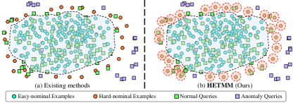
Figure 1: Visualization of training data (ball) and queries (cube) via t-SNE Van der Maaten and Hinton (2008). Visually, existing methods’ decision boundaries are predominated by the overwhelming number of easy-nominal examples (blue balls). Hence, the normal queries (green cubes) nearby the hard-nominal examples (orange balls) are prone to be erroneously identified as anomalies (purple cubes), resulting in high false-positive or missed-detection rates. To address this issue, we propose HETMM to construct a robust prototype-based decision boundary, which is capable to distinguish hard-nominal examples from anomalies.

• We observed that existing methods’ decision boundaries are predominated by easy-nominal example overwhelming, and thus hard-nominal examples are prone to be confused with anomalies, leading to high false-positive or missed-detection rates. To address this issue, we propose a simple yet efficient method dubbed Hard Nominal Example-aware Template Mutual Matching (HETMM), which is capable to construct a robust prototype-based decision boundary to distinguish hard-nominal examples from anomalies.

• We present Pixel-level Template Selection (PTS) to meet the speed-accuracy demand in practical production, which streamlines the original template set by selecting significant prototypes to form a tiny set. Unlike mainstream methods that only consider cluster centres, PTS further selects hard-nominal examples to persist the original decision boundary.

• Comprehensive experimental results and in-depth analysis on five real-world datasets show that HETMM favourably surpasses the state-of-the-art methods, particularly achieving much fewer false-positive and missed-detection rates. Moreover, using a 60-sheet template set compressed by PTS can achieve superior anomaly detection performance to existing advances under a real-time speed (26.1 FPS) on a single Quadro 8000 RTX. Additionally, HETMM can be hot updated by directly inserting novel samples into the template set, which may promptly address some incremental learning issues.

2 Related Works

2.1 Anomaly Detection

The landscape of anomaly detection methods has dramatically evolved over the past decades. Some surveys Pimentel et al (2014); Ehret et al (2019); Chalapathy and Chawla (2019) give comprehensive literature reviews. In this section, we briefly introduce some state-of-the-art approaches for subsequent comparisons.

SVDD-based Methods. Based on the assumption that the distribution of normal images is significantly different from that of anomalies, Tax and Duin Tax and Duin (2004) proposed the Support Vector Data Description (SVDD) algorithm to construct a nominal decision boundary using hand-crafted support vectors extracted from normal images. However, to improve its performance, subsequent researchers have proposed modifications. Banerjee et al. Banerjee et al (2007) introduced an improved version of the original SVDD algorithm that is faster. To construct a more accurate decision boundary, Ruff et al. Ruff et al (2018) replaced the hand-crafted support vectors with deep features. Although these modifications have led to better results, the distinction between anomalies and normal samples at the image level is often subtle. To address this issue, Yi and Yoon Yi and Yoon (2020) proposed constructing patch-level SVDD models that can discriminate anomalies based on the patch-level differences between query images and patch-level support vectors.

Reconstruction-based Methods. Relying on defect-free images to model a latent distribution of nominal data, reconstruction-based methods leverage the distribution gap between nominal and anomalous patterns to locate anomalous regions. Bergmann et al. Bergmann et al (2018) have proposed enhancing Convolutional Auto-Encoders (CAEs) Goodfellow et al (2016) segmentation results by incorporating structural similarity loss Zhao et al (2015). In contrast, Schlegl et al. Schlegl et al (2017) were the first to use Generative Adversarial Networks (GANs) Goodfellow et al (2014) to address the anomaly detection problem. To improve the effectiveness of Schlegl et al (2017), Akcay et al. Akcay et al (2018) and Schlegl et al. Schlegl et al (2019) have proposed an additional encoder to explore the latent representation for better reconstruction quality. Unlike the above-mentioned methods, Bergmann et al (2020) reconstructs the nominal features selected by teacher networks that are pre-trained on ImageNet Deng et al (2009). To incorporate global contexts into local regions, Wang et al. Wang et al (2021) have integrated the information obtained from global and local branches simultaneously, while Salehi et al (2021) aggregates hierarchical information from different resolutions. Bergmann et al. Bergmann et al (2022) have leveraged regression networks to capture global context and local patch information from a pre-trained feature encoder. However, the above methods’ decision boundaries are dominated by the overwhelming presence of easy-nominal examples, they are vulnerable to mistaking the queries nearby hard-nominal examples for anomalous queries.

Template-based Methods. In addition to the reconstruction-based approaches discussed above, another solution for anomaly detection is constructing a template set with nominal features. Nominal and anomalous features, although extracted by the same feature descriptors, significantly differ in feature representations. Therefore, distinguishing between nominal and anomalous patterns is achievable by matching queries with the template set. Cohen and Hoshen Cohen and Hoshen (2020) constructed a template set of nominal features by extracting the backbone pre-trained on ImageNet Deng et al (2009) for anomaly detection and localization. At test time, Cohen and Hoshen (2020) localizes the anomalous patterns with a $K$th Nearest Neighbor ($K$-NN) algorithm on the nominal template set. The inference complexity of Cohen and Hoshen (2020) is linear to the template set size due to the use of the $K$-NN algorithm. To reduce the inference complexity of querying the template set, Defard et al. Defard et al (2021) propose to generate patch embeddings for anomaly localization. Reiss et al. Reiss et al (2021) also propose an adaptation strategy to finetune the pre-trained features with the corresponding anomaly datasets to obtain high-quality feature representations. Additionally, PatchCore Roth et al (2022) improves Defard et al (2021)’s patch embeddings by extracting neighbour-aware patch-level features and subsampling the template set for speed-up. Similar to the reconstruction-based methods, the queries close to hard-nominal examples are also prone to be erroneously identified as anomalies by the above template-based methods, yielding high false-positive or missed-detection rates.

2.2 Multi-Prototype Representation

Multi-prototype representation algorithms aim to select $K$ prototypes to represent the distribution of $N$ samples ($K\leq N$). K-Means-type algorithms MacQueen (1967); Bezdek et al (1984) attempt to find an optimal partition of the original distribution into $K$ cluster centroids. Liu et al. Liu et al (2009) separate the samples into several regions by squared-error clustering and group each high-density region into one prototype. Nie et al. Li et al (2020) select $K$ prototypes by using a scalable and parameter-free graph fusion scheme. Additionally, since coreset Har-Peled and Kushal (2005) has been commonly used in K-Means-type algorithms, Roth et al. Roth et al (2022) propose a coreset-based selection strategy to find $K$ representatives. While the multi-prototype representation methods discussed above can effectively cover the distribution of most samples, the coverage of the hard-nominal examples is disregarded by those methods. Consequently, the tiny template set compressed by those methods may struggle to cover the distribution of hard-nominal examples.

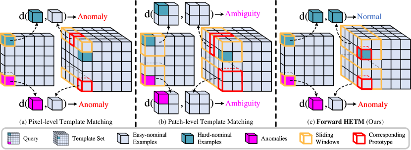
Figure 2: Visual examples of different template matching approaches. As shown, pixel- and patch-level template matching are vulnerable to confusing hard-nominal examples (blue cubes) with anomalies (pink cubes). (a) As affected by slight affine transformations, pixel-level template matching may miss the corresponding prototypes (red frames) of hard-nominal examples. (b) Although patch-level template matching has good robustness against affine transformations, the subtle anomalous signals may be covered by the overwhelming number of easy-nominal examples (grey cubes) within the patch. By contrast, the forward HETM matches the corresponding pixel-level prototypes within a patch range, which is capable of precisely distinguishing between hard-nominal examples and anomalies.

3 Methodology

In this section, we first introduce the preliminary of industrial anomaly detection. Then we show technical details of the proposed Hard Nominal Example-aware Template Mutual Matching (HETMM) and Pixel-level Template Selection (PTS). Finally, we describe the overall architecture and how to obtain anomaly detection and localization results.

3.1 Preliminary

Industrial anomaly detection aims to identify the unknown defects by the collected $N$ non-defective images $\mathcal{Z}=\{z_{i}\}^{N}_{i=1}$. Based on the prior hypotheses that most anomalies are significantly different from normal samples, provided a query image $q$ is dissimilar to all the images in $\mathcal{Z}$, it tends to be an anomaly. Intuitively, with a pre-trained network $\phi$, $q$ can be identified by

$$Cat.\!\!=\!\!\begin{cases}Normality&\!\!\!\!\inf\limits_{z_{i}\in\mathcal{Z}}\!\left\{d\left(\phi(q),\phi(z_{i})\right)\right\}\!<\!\epsilon\\ Anomaly&\!\!\!\!otherwise\end{cases}\!\!,$$ (1)

where $d(\cdot,\cdot)$ and $\epsilon$ denote distance function and anomaly decision threshold, respectively. In essence, for each query, the above template matching attempts to find the corresponding prototypes, and then calculate the distance between themselves as an anomaly score. Existing template-based anomaly detectors Cohen and Hoshen (2020); Defard et al (2021); Roth et al (2022) propose a two-stage framework: I) template generation and II) anomaly prediction, to employ template matching for anomaly detection. In stage I, these methods construct a template set $\mathcal{T}$ with a pre-trained network $\phi$:

$$\mathcal{T}=\left\{\phi(z_{1})\cup\cdots\phi(z_{i})\cup\cdots\phi(z_{N}):z_{i}\in\mathcal{Z}\right\}.$$ (2)

In stage II, for each query image $q$, these methods employ template matching to calculate its anomaly score, then identify its category by the threshold determination like Eq. 1. As a result, these template-based methods build a prototype-based decision boundary to distinguish between nominal and anomalous queries.

3.2 Hard Nominal Example-aware Template Mutual Matching

Template-based methods aim to construct a prototype-based decision boundary to detect anomalies from query samples like Eq. 1. Existing template-based methods are based on two template-matching strategies: pixel- and patch-level template matching. However, the decision boundaries built by those approaches are generally not robust. Figure 2 depicts the limitations of pixel-level template matching (a) and patch-level template matching (b). As shown, pixel-level template matching is susceptible to affine transformations, resulting in high false alarms. Although Patch-level template matching has good robustness against affine transformations, it may lead to missed detection due to easy-nominal example overwhelming.

To address the above limitations, we propose HETMM, a mutual matching between queries $Q$ and the template set $\mathcal{T}$, to construct a robust prototype-based decision boundary. Specifically, HETMM comprises forward and backward Hard Nominal Example-aware Template Matching (HETM) modules, aggregating the anomaly scores towards the forward direction (from $Q$ to $\mathcal{T}$) and backward direction (from $\mathcal{T}$ to $Q$).

Forward HETM. Let $\mathcal{P}^{\mathcal{T}}_{x,y}$ denote the elements of the template set $\mathcal{T}$ within a $n\!\times\!m$ patch centred by the given pixel $(x,y)$ formulated as

$$\mathcal{P}^{\mathcal{T}}_{x,y}\!\!=\!\!\{\mathcal{T}_{x+a,y+b}\!\!:\!\lvert a\rvert\!\leq\!\lfloor\!\frac{m}{2}\!\rfloor\!\land\!\lvert b\rvert\!\leq\!\lfloor\!\frac{n}{2}\!\rfloor,\ \!a,\!b\in\mathbb{Z}\},$$ (3)

where $(x+a,y+b)$ denotes the position indices of the patch. Given a query pixel $Q_{x,y}$, the forward HETM searches for the corresponding prototypes from $\mathcal{P}^{\mathcal{T}}_{x,y}$ and calculate anomaly score by

$$\overset{\to}{\mathbb{D}}(Q_{x,y},\mathcal{T})=\inf\limits_{\hat{p}\in\mathcal{P}^{\mathcal{T}}_{x,y}}\left\{1-\frac{Q_{x,y}\cdot\hat{p}^{\top}}{\|Q_{x,y}\|_{2}\ \|\hat{p}\|_{2}}\right\}.$$ (4)

Figure 2 (c) shows a visual example of the forward HETM. As shown, the forward HETM can construct a robust decision boundary, which is capable to alleviate the affection brought by affine transformations and easy-nominal example overwhelming.

Backward HETM. However, the forward HETM is an asymmetric distance that cannot satisfy the distance axioms, which may miss some other types of anomalies. As reported in Bergmann et al (2022), anomalies can be split into two categories: structural and logical anomalies. Structural anomalies are invalid objects dissimilar to the template set, while logical ones are the valid query objects that occur in invalid locations. Since the forward HETM can only identify whether an object is valid but fail to discover whether a valid object occurs in invalid positions, it leads to missed detection of logical anomalies. Motivated by that, we further present the backward HETM, i.e., employing HETM from $\mathcal{T}$ to $Q$ to discover whether the valid queries occur in the position. Given a query $Q_{x,y}$, backward HETM calculate its logical anomaly socre by

$$\overset{\leftarrow}{\mathbb{D}}(Q,\mathcal{T}_{x,y})=\!\!\!\inf\limits_{\tilde{p}\in\mathcal{P}^{Q}_{x,y}}\!\left\{1\!-\!\!\sup\limits_{\tilde{t}\in\mathcal{T}_{x,y}}\!\left\{\frac{\tilde{t}\cdot\tilde{p}^{\top}}{\|\tilde{t}\|_{2}\ \|\tilde{p}\|_{2}}\right\}\!\right\},$$ (5)

where $\mathcal{P}^{Q}_{x,y}$ denotes the query $Q$’s elements within a $n\!\!\times\!\!m$ patch centred by the given pixel $(x,y)$.

Given the structural anomaly score $\overset{\to}{\mathbb{D}}(Q_{x,y},\mathcal{T})$ and logical anomaly score $\overset{\leftarrow}{\mathbb{D}}(Q,\mathcal{T}_{x,y})$, HETMM calculates the final anomaly score by

$$\mathbb{D}^{\dagger}\!(Q_{x,y},\!\!\mathcal{T}_{x,y})\!=\!\alpha\overset{\rightarrow}{\mathbb{D}}(Q_{x,y},\!\!\mathcal{T})\!+\!(1-\alpha)\overset{\leftarrow}{\mathbb{D}}(Q,\!\!\mathcal{T}_{x,y}),$$ (6)

where $\alpha$ denotes the ratio to balance the signals of structural and logical anomalies. Figure 3 depicts the inner architecture of the proposed HETMM. As shown, the anomaly maps obtained by forward and backward HETM can capture structural and logical anomalies, respectively. Moreover, the final anomaly map achieves high-quality defect segmentation performance, which convincingly confirms the correctness of our motivation.

3.3 Pixel-level Template Selection

For each query, HETMM aims to identify its category by measuring the distance between itself and the template set $\mathcal{T}$. Hence, an ideal template set is supposed to represent the distribution of all the normal samples. However, since industrial images have considerable redundant features, the ideal template set should consist of vast images, leading to considerable computational costs in template matching. Therefore, to meet the speed-accuracy demand for industrial production, we can construct a tiny set $\mathcal{T}^{K}$ to represent the distribution of the original template set $\mathcal{T^{*}}$ by selecting $K$ prototypes from $N$ ones ($K\leq N$).

To streamline the original template set $\mathcal{T^{*}}$ into a tiny set $\mathcal{T}^{K}$, two frequently-used manners of selecting $K$ prototypes are random policy and $K$-Means MacQueen (1967). Random policy means randomly selecting a fraction of data from $\mathcal{T^{*}}$. Despite computational cost decrease, its representation capability is neither satisfactory nor stable. In practical tasks, the clustering centroids of $K$-Meansare are often used for distribution representation. Figure 4 (a) and (b) visualize the multi-prototype representation results of random selection and $K$-Means, respectively. As expected, the distribution of random selection is rambling. By contrast, the prototypes selected by $K$-Means obtain an acceptable representation performance, which covers most easy-nominal examples. However, the hard-nominal examples receive little consideration from $K$-Means. Consequently, the tiny set compressed by $K$-Means cannot persist the original boundaries, and thus hard-nominal queries tend to be error-detected as anomalies, leading to false positives.

To achieve a comparable distribution and persist decision boundaries against the original template $\mathcal{T}^{*}$, we argue that not only easy-nominal prototypes but some hard-nominal ones are also required. Therefore, we present Pixel-level Template Selection (PTS) module to select some hard-nominal prototypes from $\mathcal{T}^{*}$ after containing sufficient easy-nominal prototypes. Precisely, PTS consists of two steps: I) easy-nominal example-based initialization and II) hard-nominal prototype selection. Alg.1 describes the detailed algorithm procedure of the proposed PTS.

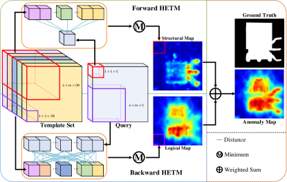
Figure 3: The inner structure of HETMM. For each query image, its structural and logical anomaly map is generated by forward and backward HETM, respectively. The final anomaly map is the weighted sum of these two maps.

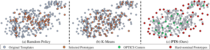
Figure 4: The visualization of multi-prototype representation results over the original template set (grey balls) via t-SNE Van der Maaten and Hinton (2008). Visually, the prototypes selected by random policy (a) are rambling, while $K$-Means (b) only collect easy-nominal prototypes. By contrast, PTS (c) achieves a better distribution coverage of the original template set, collecting OPTICS Ankerst et al (1999) centres (green balls) and hard-nominal prototypes (red balls) to persist the original decision boundaries.

Easy-nominal Example-based Initialization. Let $(x,y)$ denote the pixel coordinate, for each $\mathcal{T}^{K}_{x,y}$, PTS first employs the density clustering method OPTICS Ankerst et al (1999) to find the easy-nominal examples from $\mathcal{T}^{*}_{x,y}$. These easy-nominal examples are split into several high-density regions $\mathcal{R}=\{r_{i}\}_{i=1}^{M}$, where $M$ indicates the number of regions. For each region $r_{i}$, since the easy-nominal examples in $r_{i}$ are close to each other, the region centre $t_{i}$ can be regarded as an easy-nominal prototype, which can be formulated by

$$t_{i}=\mathop{\arg\max}_{w\in r_{i}}\left\{\sum_{\hat{w}\in r_{i}}\frac{w\cdot\hat{w}^{\top}}{\|w\|_{2}\ \|\hat{w}\|_{2}}\right\}.$$ (7)

If OPTICS fails to find any high-density regions, which means the features in $\mathcal{T}^{*}_{x,y}$ are scattered each other, and thus $\mathcal{T}^{K}_{x,y}$ can be initialized by the global centre $t_{g}$ formulated as

$$t_{g}=\mathop{\arg\max}\limits_{w\in\mathcal{T}^{*}_{x,y}}\left\{\sum\limits_{\tilde{w}\in\mathcal{T}^{*}_{x,y}}\frac{w\cdot\tilde{w}^{\top}}{\|w\|_{2}\ \|\tilde{w}\|_{2}}\right\}.$$ (8)

Hence, $\mathcal{T}^{K}_{x,y}$ can be initialized by the aggregation of these selected easy-nominal prototypes.

Hard-nominal Prototype selection. Since $\mathcal{T}^{K}_{x,y}$ is initialized by a set of easy-nominal prototypes, the easy-nominal examples are close to $\mathcal{T}^{K}_{x,y}$ while the hard-nominal ones are not. Therefore, we can find the hard-nominal prototypes from $\mathcal{T}^{*}_{x,y}$ according to the distance between each prototype and $\mathcal{T}^{K}_{x,y}$. Specifically, a hard-nominal prototype $t_{h}$ is selected by the highest cosine distance in every iteration, which can be formulated as

$$t_{h}=\!\!\mathop{\arg\max}_{w\in\mathcal{T}^{*}_{x,y}\setminus\mathcal{T}^{K}_{x,y}}\!\left\{\sum_{\tilde{w}\in\mathcal{T}^{K}_{x,y}}\!\left(1-\frac{w\cdot\tilde{w}^{\top}}{\|w\|_{2}\ \|\tilde{w}\|_{2}}\right)\!\right\}.$$ (9)

The distribution coverage of PTS is shown in Figure 4 (c). Visually, easy-nominal prototypes selected in step I cover the most samples inner the original distribution. Moreover, the hard-nominal examples scattered at the boundary of the original distribution are also well-covered by the hard-nominal prototypes selected in step II. Compared to the results of random policy and $K$-Means, PTS achieves better representation performance, especially maintaining the original decision boundaries.

Input: Original template set pixels $\mathcal{T}^{*}_{x,y}$, sheets $K$, OPTICS $\psi(\cdot)$

Output: Tiny template set pixels $\mathcal{T}^{K}_{x,y}$.

/* Step I. Initialization. */

1 Get high-density regions $\mathcal{R}\leftarrow\psi(\mathcal{T}_{x,y})$;

2 if $len(\mathcal{R})>0$ then

3       Tiny template set initialization: $\mathcal{T}^{K}_{x,y}\leftarrow\{\}$;

4       for $r_{i}\in\mathcal{R}$ do

5             Get easy-nominal prototypes $t_{i}$ by Eq. 7;

6             Update tiny template set: $\mathcal{T}^{K}_{x,y}\leftarrow\mathcal{T}^{K}_{x,y}\cup\{t_{i}\}$;

7            

8       end for

9      

10else

11       Get global center $t_{g}$ by Eq. 8;

12       Tiny template set initialization: $\mathcal{T}^{K}_{x,y}\leftarrow\{t_{g}\}$;

13      

14 end if

/* Step II. Selection. */

15 while $len(\mathcal{T}^{K}_{x,y})<K$ do

16       Get hard-nominal prototypes $t_{h}$ by Eq. 9;

17       Update tiny template set: $\mathcal{T}^{K}_{x,y}\leftarrow\mathcal{T}^{K}_{x,y}\bigcup\{t_{h}\}$;

18      

19 end while

Algorithm 1 Process of PTS.

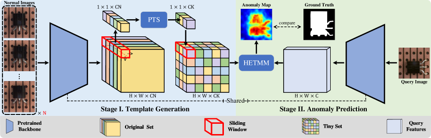
Figure 5: The overall framework of our methods. In stage I, the original template set $\mathcal{T}^{*}$ is the aggregation of the features extracted from the collected $N$ nominal-only images $\mathcal{Z}$ by a pre-trained backbone $\phi$. To streamline $\mathcal{T}^{*}$ into a tiny set $\mathcal{T}^{K}$ with $K$ sheets ($N\geq K$), PTS selects $K$ significant prototypes from $\mathcal{T}^{*}$ in each pixel coordinate. In stage II, given a query image $q$, we first extract its feature $Q$ by the same pre-trained backbone $\phi$ and then employ HETMM to obtain the corresponding anomaly map.

3.4 Overall Framework

The overall framework of our methods is illustrated in Figure 5. Similar to the existing template-based methods Cohen and Hoshen (2020); Roth et al (2022), the proposed framework also comprises two stages: I) template generation, II) anomaly prediction, as reported in Section 3.1. In stage I, given the original template set $\mathcal{T}^{*}$, we employ the PTS to compress $\mathcal{T}^{*}$ into a $K$-sheet tiny set $\mathcal{T}^{K}$. In stage II, for each query image $q$, we first extract its feature $Q$ by the same pre-trained model $\phi$. Then, the anomaly map is obtained by employing HETMM to calculate the anomaly scores for every pixel of the query features $Q$. Specifically, to capture the multi-layer contextual information for precise anomaly localization, we collect the hierarchical anomaly maps $\mathcal{M}^{s}$ obtained from multiple layers. Let $s_{i}$ denote the anomaly map obtained from the $i$th layer, the final results $S$ can be calculated by

$$S=\sum_{s_{i}\in\mathcal{M}^{s}}\varphi(s_{i},\xi),$$ (10)

where $\varphi(\cdot,\xi)$ denotes the rescale operation to upsample the anomaly maps with the $\xi$ resolutions, while the default value of $\xi$ equals the resolution of the query image $q$.

3.5 Detection and Localization

Given the final anomaly map $S$ by integrating each anomaly map $s_{i}$ in Eq. 10, we can obtain anomaly detection and localization results by some frequently-used post-processing techniques. Following the previous works Roth et al (2022); Cohen and Hoshen (2020); Defard et al (2021), the anomaly detection results $S^{D}$ are calculated by

$$S^{D}=\varPhi(\mathcal{G}(S,\sigma)),$$ (11)

where $\mathcal{G}(\cdot,\sigma)$ denotes the Gaussian blur filter with $\sigma=6.8$, while $\varPhi$ indicates the global maximum operation. For anomaly localization result $S^{L}$, it can be directly obtained by employing the 0-1 normalization operation to the anomaly map $S$ without demanding other post-processing techniques.

Table 1: Quantitative comparisons of start-of-the-arts on MVTec AD dataset in terms of the AUROC % for image-level anomaly detection in this table. Bold and underline texts indicate the best and second best performance.

Category		P-SVDDYi and Yoon (2020)	USBergmann et al (2020)	PadimDefard et al (2021)	DifferNetRudolph et al (2021)	CutPasteLi et al (2021)	GLFCWang et al (2021)	MKDSalehi et al (2021)	DRAEMZavrtanik et al (2021)	PatchCoreRoth et al (2022)	HETMM	HETMM
		(ACCV’20)	(CVPR’20)	(ICPR’21)	(WACV’21)	(CVPR’21)	(CVPR’21)	(CVPR’21)	(ICCV’21)	(CVPR’22)	(ALL)	(60 sheets)
Textures	carpet	92.9	91.6	99.8	92.9	93.1	92.0	79.3	97.0	98.0	100.0	99.8
	grid	94.6	81.0	96.7	84.0	99.9	67.0	78.0	99.9	98.6	99.9	99.9
	leather	90.9	88.2	100.0	97.1	100.0	83.0	95.0	100.0	100.0	100.0	100.0
	tile	97.8	99.1	98.1	99.4	93.4	97.0	91.6	99.6	99.4	100.0	99.9
	wood	96.5	97.7	99.2	99.8	98.6	100.0	94.3	99.1	99.2	98.8	99.0
Objects	bottle	98.6	99.0	99.9	99.0	98.3	99.0	99.4	99.2	100.0	100.0	100.0
	cable	90.3	86.2	92.7	95.9	80.6	98.0	89.2	91.8	99.3	100.0	100.0
	capsule	76.7	86.1	91.3	86.9	96.2	79.0	80.5	98.5	98.0	97.9	99.3
	hazelnut	92.0	93.1	92.0	99.3	97.3	99.0	98.4	100.0	100.0	100.0	100.0
	metal nut	94.0	82.0	98.7	96.1	99.3	85.0	82.4	98.7	99.7	100.0	100.0
	pill	86.1	87.9	93.3	88.8	92.4	82.0	82.7	98.9	97.0	96.6	97.0
	screw	81.3	54.9	85.8	96.3	86.3	87.0	83.3	93.9	96.4	97.4	94.1
	toothbrush	100.0	95.3	96.1	98.6	98.3	92.0	92.2	100.0	100.0	100.0	98.9
	transistor	91.5	81.8	97.4	91.1	95.5	97.0	85.6	93.1	99.9	100.0	100.0
	zipper	97.9	91.9	90.3	95.1	99.4	100.0	93.2	100.0	99.2	98.2	96.7
Average		92.1	87.7	95.5	94.9	95.2	91.0	87.7	98.0	99.0	99.3	99.0

Table 2: Quantitative comparisons of start-of-the-arts on MVTec AD dataset in terms of the AUROC % for pixel-level anomaly localization in this table. Bold and underline texts indicate the best and second best performance.

Category		P-SVDDYi and Yoon (2020)	USBergmann et al (2020)	PadimDefard et al (2021)	PANDAReiss et al (2021)	CutPasteLi et al (2021)	GLFCWang et al (2021)	MKDSalehi et al (2021)	DRAEMZavrtanik et al (2021)	PatchCoreRoth et al (2022)	HETMM	HETMM
		(ACCV’20)	(CVPR’20)	(ICPR’21)	(CVPR’21)	(CVPR’21)	(CVPR’21)	(CVPR’21)	(ICCV’21)	(CVPR’22)	(ALL)	(60 sheets)
Textures	carpet	96.0	93.5	99.0	97.5	92.6	98.3	95.6	95.5	98.9	99.2	99.1
	grid	96.2	89.9	97.1	93.7	97.5	78.0	91.8	99.7	98.6	99.2	98.6
	leather	97.4	97.8	99.0	97.6	99.5	90.0	98.0	98.6	99.3	99.6	99.5
	tile	91.4	92.5	94.1	87.4	90.5	80.0	82.8	99.2	96.1	96.0	96.0
	wood	90.8	92.1	94.1	88.5	95.5	81.0	84.8	96.4	95.1	95.6	95.6
Objects	bottle	98.1	97.8	98.2	98.4	97.6	93.0	96.3	99.1	98.5	98.6	98.6
	cable	96.8	91.9	96.7	97.2	90.0	94.0	82.4	94.7	98.2	98.4	98.4
	capsule	95.8	96.8	98.6	99.0	97.4	90.0	95.9	94.3	98.8	98.4	98.3
	hazelnut	97.5	98.2	98.1	99.1	97.3	84.0	94.6	99.7	98.6	99.3	99.2
	metal nut	98.0	97.2	97.3	98.1	93.1	91.0	86.4	99.5	98.4	97.4	96.8
	pill	95.1	96.5	95.7	96.5	95.7	93.0	89.6	97.6	97.1	97.8	97.7
	screw	95.7	97.4	98.4	98.9	96.7	96.0	96.0	97.6	99.2	99.5	98.8
	toothbrush	98.1	97.9	98.8	97.9	98.1	96.0	96.1	98.1	98.5	99.1	99.1
	transistor	97.0	73.7	97.6	94.1	93.0	100.0	76.5	90.9	94.9	96.5	97.4
	zipper	95.1	95.6	98.4	96.5	99.3	99.0	93.9	98.8	98.8	98.3	98.1
Average		95.7	93.9	97.4	96.2	96.0	91.0	90.7	97.3	98.0	98.2	98.1

4 Experiments & Analysis

In this section, we conduct extensive experiments and in-depth analyses to demonstrate the superiority of the proposed methods in anomaly detection and localization. Following the one-class classification protocols, we only leverage normal images to detect and localize unknown anomalies.

4.1 Experimental Details

Datasets. We comprehensively compare our methods and the state-of-the-art approaches on the following 5 real-world datasets (4 industrial datasets and 1 non-industrial dataset). The comprehensive evaluation on the MVTec AD dataset is reported in Sec 4.2, while the other 4 datasets are evaluated in Sec 4.3.

MVTec Anomaly Detection (MVTec AD) benchmark Bergmann et al (2019) consists of 15 categories with a total of 5354 high-resolution images, of which 3629 anomaly-free images are used for training and the rest 1725 images, including normal and anomalous ones for testing. Each category owns 60 to 390 nominal-only training images, and both image- and pixel-level annotations are provided in its test set. As a real-world industrial dataset, most of our experiments are conducted on MVTec AD to evaluate industrial anomaly detection and localization performance.

Magnetic Tile Defects (MTD) dataset Huang et al (2020), a specialized real-world industrial dataset for the detection of magnetic tile defects. MTD contains 952 defect-free images, the rest 395 defective magnetic tile images with various illumination levels split into $5$ defect types. Following the setting reported in Rudolph et al (2021), we select 80% nominal magnetic tile images as nominal-only training data, the rest 20% images for the test. The experiments performed on MTD can demonstrate the models’ capability of detecting anomalies in various illuminative environments.

MVTec Logical Constraints Anomaly Detection (MVTec LOCO AD) Bergmann et al (2022) is the latest anomaly detection dataset with 3644 real-world industrial images, of which 1772 anomaly-free images for training, 304 anomaly-free images for validation and the rest (575 anomaly-free and 993 defective images) belong to the test set. It consists of 5 object categories from industrial inspection scenarios. Unlike the one-class-classification settings, MVTec LOCO AD employs a two-class classification, classifying various defects into 2 categories: structural and logical anomalies. Compared to the existing anomaly detection dataset, the performance evaluated on MVTec LOCO AD is more emphasis on global contexts.

MVTec Structural and Logical Anomaly Detection (MVTec SL AD) Bergmann et al (2022) is a dataset that employs the above two-class classification settings on the original MVTec AD. There are only 3 categories containing 37 logical anomalous images in a total of 1258 anomaly images, while the rest are structural ones.

Mini Shanghai Tech Campus (mSTC) Liu et al (2018) dataset is an abnormal event dataset. Following the settings reported in Venkataramanan et al (2020); Defard et al (2021); Roth et al (2022), we subsample the original Shanghai Tech Campus (STC) dataset by extracting every fifth training and test video frame. In 12 scenes, mSTC’s training data are the normal pedestrian behaviours, while the abnormal behaviours, such as fighting or cycling, belong to its test set. Compared to the above industrial datasets, localizing the abnormal events is a long-range spatiotemporal challenge.

Table 3: Quantitative comparisons of start-of-the-arts on MVTec AD dataset in terms of the PRO % for pixel-level anomaly localization in this table. Bold and underline texts indicate the best and second best performance.

Category		OCSVMAndrews et al (2016)	AnoGANSchlegl et al (2017)	1-NNNazare et al (2018)	SSIM-AEBergmann et al (2018)	${l_{2}}$-AEBergmann et al (2018)	SPADECohen and Hoshen (2020)	USBergmann et al (2020)	PadimDefard et al (2021)	PatchCoreRoth et al (2022)	HETMM	HETMM
		(JMLR’16)	(IPMI’17)	(arXiv’18)	(arXiv’18)	(arXiv’18)	(arXiv’20)	(CVPR’20)	(ICPR’21)	(CVPR’22)	(ALL)	(60 sheets)
Textures	carpet	35.5	20.4	51.2	64.7	45.6	94.7	69.5	96.2	96.5	96.8	96.4
	grid	12.5	22.6	22.8	84.9	58.2	86.7	81.9	94.6	96.1	97.0	95.4
	leather	30.6	37.8	44.6	56.1	81.9	97.2	81.9	97.8	98.9	98.6	98.5
	tile	72.2	17.7	82.2	17.5	89.7	75.6	91.2	86.0	88.3	88.5	88.2
	wood	33.6	38.6	50.2	60.5	72.7	87.4	72.5	91.1	89.5	93.6	93.6
Objects	bottle	85.0	62.0	89.8	83.4	91.0	95.5	91.8	94.8	95.9	96.0	96.0
	cable	43.1	38.3	80.6	47.8	82.5	90.9	86.5	88.8	91.6	95.4	95.0
	capsule	55.4	30.6	63.1	86.0	86.2	93.7	91.6	93.5	95.5	95.4	95.6
	hazelnut	61.6	69.8	86.1	91.6	91.7	95.4	93.7	92.6	93.8	96.9	96.8
	metal nut	31.9	32.0	70.5	60.3	83.0	94.4	89.5	85.6	91.2	95.3	94.2
	pill	54.4	77.6	72.5	83.0	89.3	94.6	93.5	92.7	92.9	97.1	96.9
	screw	64.4	46.6	60.4	88.7	75.4	96.0	92.8	94.4	97.1	97.3	95.9
	toothbrush	53.8	74.9	67.5	78.4	82.2	93.5	86.3	93.1	90.2	93.8	93.7
	transistor	49.6	54.9	68.0	72.5	72.8	87.4	70.1	84.5	81.2	92.3	94.1
	zipper	35.5	46.7	51.2	66.5	83.9	92.6	93.3	95.9	97.0	96.0	95.7
Average		47.9	44.3	64.0	69.4	79.0	91.7	85.7	92.1	93.1	95.4	95.1

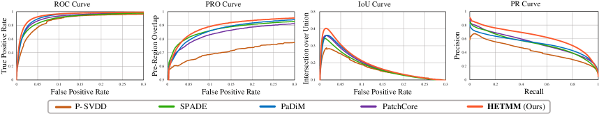
Figure 6: Different curves of the proposed 60-sheet HETMM and state-of-the-art methods on MVTec AD.

Evaluation Metrics. Following the settings of recent anomaly detection methods Bergmann et al (2020); Roth et al (2022), we employ the Area Under the Receiver Operating Characteristic Curve (AUROC) and the Per-Region Overlap (PRO) Bergmann et al (2019) metrics for evaluations. The image- and pixel-level AUROC are employed to measure the performance of image-level anomaly detection and pixel-level anomaly localization, respectively. In addition, we use the PRO to further evaluate the anomaly localization quality. Let $C_{i,k}$ denote the anomalous regions for a connected component $k$ in the ground truth image $i$ and $P_{i}$ denote the predicted anomalous regions for a threshold $t$. Then, the PRO can be formulated as

$$PRO=\frac{1}{N}\sum_{i}\sum_{k}\frac{|P_{i}\cap C_{i,k}|}{|C_{i,k}|},$$ (12)

where $N$ is the number of ground truth components. As proposed in Bergmann et al (2020), We average the PRO score with false-positive rates below 30%. Therefore, a higher PRO score indicates that anomalies are well-localized with lower false-positive rates.

Implementation Details. Our experiments are based on Pytorch Paszke et al (2017) framework and run with a single Quadro 8000 RTX. $\phi$ here represents the WResNet101 Zagoruyko and Komodakis (2016) backbone pre-trained on ImageNet Deng et al (2009) without fine-tuning. The OPTICS algorithm we used is re-implemented by scikit-learn Pedregosa et al (2011). Following the settings in Li et al (2021), we rescale all the images into 256$\times$256 in our experiments. Since class-specific data augmentations require prior knowledge of inspected items, we do not use any data augmentation techniques for fair comparisons.

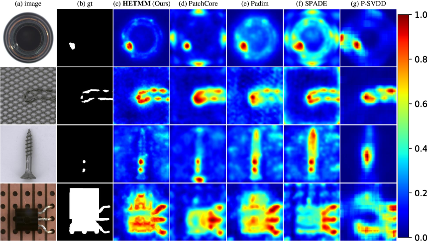
Figure 7: Visual comparisons between the proposed 60-sheet HETMM and other state-of-the-arts on the MVTec AD dataset.

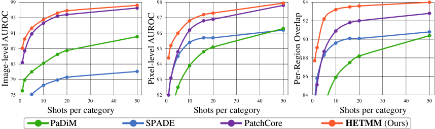
Figure 8: The sample-efficiency visualizations for anomaly detection and localization on the MVTec AD dataset.

4.2 Evaluations on MVTec AD

In this subsection, we comprehensively compare the proposed HETMM and 16 state-of-the-art methods, especially the recent benchmark (PatchCore Roth et al (2022)), for anomaly detection and localization on the MVTec AD dataset. We evaluate two different template sets: the original template set and the 60-sheet tiny set compressed by PTS, which is indicated by ALL and 60 sheets, respectively. The patch sizes in Eq. 3 are set to 9$\times$9, 7$\times$7 and 5$\times$5 corresponding to the hierarchical layers 1, 2 and 3 in Eq. 10, respectively. The ratio $\alpha$ in Eq. 6 is set to $0.8$ as default.

Image-level Anomaly Detection. Table 1 reports the quantitative evaluation results of image-level AUROC. As demonstrated, the average performance of the original HETMM favourably surpasses all the competitors with consistent outperformance in all categories, suggesting HETMM has good robustness in the detection of various anomalies objects. In addition, the 60-sheet HETMM achieves a comparable performance to PatchCore Roth et al (2022) and surpasses the rest compared methods by over 0.6%, which reveals PTS can reduce the computational costs with maintaining superior performance.

Pixel-level Anomaly Localization. Table 2 and 3 report the results of pixel-level AUROC and PRO, respectively. In the above tables, the original and 60-sheet HETMM favourably outperform all the exhibited methods, especially over a 2% increase in PRO metric than the third-best method (PatchCore Roth et al (2022)). According to the introduction of PRO metric in Sec 4.1, the proposed HETMM can well localize anomalies with much lower false-positive rates than competitors. Due to containing fewer false positives, anomalies can be more easy-distinguished. Therefore, HETMM achieves better anomaly localization quality. Additionally, 60-sheet HETMM is slightly inferior to the original one, suggesting the proposed PTS can tremendously maintain the anomaly localization capability.

Table 4: Quantitative comparisons of start-of-the-arts on MTD dataset in terms of the AUROC % for image-level anomaly detection in this table. Bold text indicates the best performance.

OCSVMAndrews et al (2016)	DSEBMZhai et al (2016)	GeoTransGolan and El-Yaniv (2018)	GanomalyAkcay et al (2018)	1-NNNazare et al (2018)	ADGANCheng et al (2020)	DifferNetRudolph et al (2021)	PatchCoreRoth et al (2022)	HETMM
(JMLR’16)	(ICML’16)	(NIPS’18)	(ACCV’18)	(arXiv’18)	(ITNEC’20)	(WACV’21)	(CVPR’22)	(Ours)
58.7	57.2	75.5	76.6	80.0	46.4	97.7	97.9	98.7

Table 5: Quantitative comparisons of start-of-the-arts on mSTC dataset in terms of the AUROC % for pixel-level anomaly localization in this table. Bold text indicates the best performance.

SSIM-AEBergmann et al (2018)	AVIDSabokrou et al (2018)	LSAAbati et al (2019)	$\gamma$-VAEgDehaene et al (2020)	SPADECohen and Hoshen (2020)	CAVGA-RVenkataramanan et al (2020)	PadimDefard et al (2021)	PatchCoreRoth et al (2022)	HETMM
(arXiv’18)	(ACCV’18)	(CVPR’19)	(arXiv’20)	(arXiv’20)	(ECCV’20)	(ICPR’21)	(CVPR’22)	(Ours)
68.0	70.0	71.0	75.0	89.9	85.0	91.2	91.8	93.2

Different Curves. In Figure 6, we compare the proposed HETMM with the 60-sheet template set to 4 state-of-the-art methods: P-SVDD Yi and Yoon (2020), SPADE Cohen and Hoshen (2020), Padim Defard et al (2021) and PatchCore Roth et al (2022), on MVTec AD dataset in terms of 4 curves: ROC, PRO, IoU and PR curves. The results of P-SVDD and PatchCore are obtained by their official implementation, while SPADE and Padim are implemented by the unofficial projects. As shown, 60-sheet HETMM consistently outperforms all the other methods in those four curves. The outperformance of ROC, PRO and IoU curves indicate that HETMM can precisely localize anomalies with much lower false positive rates. In addition, HETMM surpasses the other advances in the PR curve. It means our results’ boundary and anomalous region are more precise than the competitors, achieving higher precision scores in all the thresholds. Notably, our method has better discrimination between anomalies and hard-nominal examples than other competitors, yielding fewer false positives and missed-detection rates.

Table 6: Image-level AUROC comparisons between ours and the results reported in Bergmann et al (2022) on MVTec SL AD dataset. Bold text indicates the best performance.

	f-AnoGANSchlegl et al (2019)	SPADECohen and Hoshen (2020)	USBergmann et al (2020)	GCADBergmann et al (2022)	HETMM
	(MIA’19)	(arXiv’20)	(CVPR’20)	(IJCV’22)	(Ours)
$\mathcal{S}$	75.1	93.6	89.8	87.1	99.1
$\mathcal{L}$	75.1	74.7	90.6	99.1	99.8
$Avg.$	75.1	84.2	90.2	93.1	99.5

Visual Comparisons. Figure 7 visualizes the anomaly localization results of 60-sheet HETMM and other competitors. It can be observed that the proposed HETMM well localizes structural anomalies in various situations, i.e., containing the anomalies too small (rows 1), anomalies occluded by other objects (row 2), and multi-anomalies (row 3). Compared to the exhibited methods, the highlighted regions of HETMM achieve the best visual verisimilitude to the ground truths. Note that HETMM can precisely locate the logical anomalies (row 4), while only Padim Defard et al (2021) among the competitors can capture those anomalies. In conclusion, HETMM achieves better anomaly localization quality, having more precise boundaries and fewer false positives.

Inference Time. Though using the original template set achieves the best performance, its inference speed (4.7 FPS) can not satisfy the speed demands in industrial production. Thanks to the effect of PTS, the 60-sheet tiny template set can obtain comparable performance to the original one with over 5x time accelerations (26.1 FPS).

Sample Efficiency. Sample efficiency is to evaluate the performance of few-shot anomaly detection that detects and localizes anomalies by limited normal samples. For evaluation, the template set is constructed by varying the number of normal images from 1 to 50, and we randomly construct each template set 10 times to obtain the mean scores. As shown in Figure 8, HETMM favourably surpasses all the competitors, especially when the template set is constructed with fewer samples. The outperformance means that HETMM shows higher sample-efficiency capability, notably outperforming competitors under the few-shot settings. Therefore, some incremental issues may be addressed by inserting several corresponding novel samples.

Table 7: Image-level AUROC comparisons between ours and the results reported in Bergmann et al (2022) on MVTec LOCO AD dataset. Bold text indicates the best score.

	f-AnoGANSchlegl et al (2019)	SPADECohen and Hoshen (2020)	USBergmann et al (2020)	GCADBergmann et al (2022)	HETMM
	(MIA’19)	(arXiv’20)	(CVPR’20)	(IJCV’22)	(Ours)
$\mathcal{S}$	62.7	66.8	88.3	80.6	85.8
$\mathcal{L}$	65.8	70.9	66.4	86.0	82.4
$Avg.$	64.2	68.9	77.3	83.3	84.1

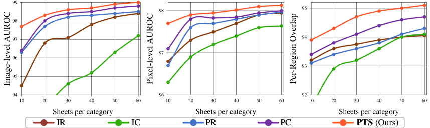
Figure 9: The multi-prototype-efficiency visualizations for anomaly detection and localization on the MVTec AD dataset.

4.3 Evaluation on other datasets

We evaluate the performance of HETMM on 4 additional anomaly detection benchmarks: The Magnetic Tile Defects (MTD) Huang et al (2020), Mini ShanghaiTech Campus (mSTC) Liu et al (2018), MVTec Structural and Logical Anomaly Detection (MVTec SL AD) Bergmann et al (2022) and MVTec Logical Constraints Anomaly Detection (MVTec LOCO AD) Bergmann et al (2022) datasets. All the images are rescaled into 256$\times$256 resolutions.

MTD. We follow the settings proposed in Rudolph et al (2021) to evaluate the anomaly detection performance in terms of the average image-level AUROC on the MTD dataset. To capture the subtle magnetic tile defects, we employ the hierarchical layers 1 and 2 with the patch sizes 3$\times$3 and 3$\times$3. Table 4 reports the evaluation results. As shown, the proposed HETMM achieves the best performance, favourably outperforming competitors over 0.8% image-level AUROC. The superior performance on MTD demonstrates that HETMM is capable of detecting anomalies in various illuminative environments.

Table 8: Performance of different template matching strategies on MVTec AD dataset. Bold text indicates the best performance.

	$point.$	$patch.$	forward HETM	HETMM
$AUC_{I}\uparrow$	95.6	98.9	99.2	99.3
$AUC_{P}\uparrow$	96.9	97.8	98.2	98.2
$PRO\uparrow$	91.2	93.4	95.4	95.4

mSTC. Following the protocols described in Sec 4.1, we evaluate the anomaly localization performance in terms of the average pixel-level AUROC on the mSTC dataset. Since the localization of abnormal events is a long-range spatiotemporal challenge, we employ the hierarchical layers 2 and 3 with the larger bi-directional patches 9$\times$9 and 5$\times$5, respectively. As reported in Table 5, the proposed HETMM achieves the best performance, surpassing the second-best method by 1.4% AUROC. Since mSTC is a non-industrial dataset, the superior performance on mSTC indicates HETMM not merely works well in industrial situations and has good transferability to various domains.

MVTec SL AD and MVTec LOCO AD. Finally, we follow the protocols reported in Bergmann et al (2022) to measure image-level anomaly detection of structural and logical anomalies. For evaluating the MVTec SL AD dataset, we adopt the same hyper-parameters in Sec 4.2. For evaluating the MVTec LOCO AD dataset, we employ the hierarchical layers 2, 3 and 4 with larger patches 11$\times$11, 9$\times$9 and 7$\times$7 in Eq. 10 for wide-range global contexts. To capture logical constraints, $\alpha$ is set to $0.6$ in Eq. 6. Table 6 and 7 report the evaluation results on MVTec SL AD and MVTec LOCO AD datasets, where $\mathcal{S}$ and $\mathcal{L}$ denote the structural and logical anomalies. As we can see, HETMM has an overwhelming superiority on the MVTec SL AD dataset, nearly 12% and 6.4% higher than the second best method on structural anomalies and average, respectively. On the MVTec LOCO AD dataset, HETMM achieves the best performance, surpassing the second-best method by 0.8% on average. The above performance on MVTec SL AD and MVTec LOCO AD datasets suggests that HETMM can capture logical constraints to detect anomalies under the structural and logical settings.

Table 9: Image-level AUROC comparisons between HETMM and its sub-modules on MVTec LOCO AD dataset. Bold text indicates the best performance.

	forward HETM	backward HETM	HETMM
$\mathcal{S}$	86.0	82.5	85.8
$\mathcal{L}$	79.7	82.7	82.4
$Avg.$	82.9	82.6	84.1

Table 10: Results of different pre-trained backbones on the MVTec AD dataset. Bold text indicates the best performance.

	ResNet18		ResNet50		ResNet101		ResNeXt50		ResNeXt101		WResNet50		WResNet101
	ALL	60 sheets	ALL	60 sheets	ALL	60 sheets	ALL	60 sheets	ALL	60 sheets	ALL	60 sheets	ALL	60 sheets
$AUC_{I}\uparrow$	98.2	97.6	98.7	98.4	98.9	98.5	98.7	98.0	99.1	98.8	99.0	98.6	99.3	99.0
$AUC_{P}\uparrow$	97.4	97.1	97.8	97.5	97.9	97.5	97.5	97.4	97.7	97.2	97.5	97.3	98.2	98.1
$PRO\uparrow$	94.0	93.2	94.5	94.0	94.7	94.4	94.6	94.1	94.5	94.0	94.5	94.1	95.4	95.1

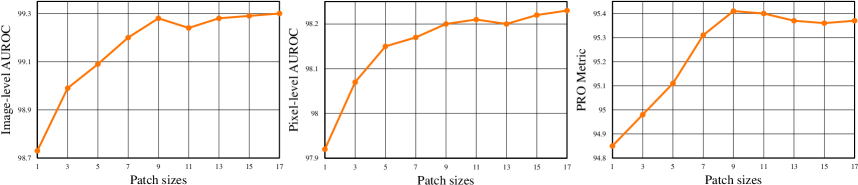
Figure 10: The performance over different patch sizes on the MVTec AD dataset.

4.4 Ablation Study and Hyper-parameter Sensitivity Analysis

In this subsection, we first conduct comprehensive ablation experiments to prove the correctness of the designs of HETMM and PTS with different template matching and template selection strategies, respectively. Subsequently, we evaluate our method under different hyper-parameters, including pre-trained backbones, patch sizes, hierarchical combinations and template sizes, to analyze the sensitivity of these hyper-parameters. $AUC_{I}$, $AUC_{P}$ and $PRO$ denote the image-level AUROC, pixel-level AUROC and the PRO metric, respectively.

Different matching strategies. We conduct experiments to prove the correctness of the designs of the proposed HETMM. Specifically, we first compare forward HETM and HETMM to the other two template matching strategies: pixel-level template matching $point.$ and patch-level template matching $patch.$ on the MVTec AD dataset. The results of Table 8 confirm the correctness of the motivations of HETMM. Point-to-point template matching has inferior robustness and achieves the worst performance among the exhibited methods. Though patch-to-patch template matching achieves acceptable performance in an image- and pixel-level AUROC, due to the easy-nominal example overwhelming, its performance is inferior to forward HETM, especially in the PRO metric. As reported in Bergmann et al (2022), the MVTec AD dataset contains few logical anomalies. Thus HETMM has slight outperformance against the forward HETM.

To evaluate the advantages of HETMM in detecting logical anomalies, we further compare HETMM to the forward and backward HETM on the MVTec LOCO AD dataset. As reported in Table 9, forward HETM achieves superior performance in detecting structural anomalies but is inferior to backward HETM on logical anomalies. It means structural and logical anomalies can be well-detected by the forward and backward HETM, respectively. Hence, by combining these bi-directional matching, HETMM achieves the optimum in detecting structural and logical anomalies.

Different selection strategies. To evaluate the effect of the proposed PTS, we conduct a series of comparisons between PTS and other template selection strategies, including random selection: image-level random selection $IR$ and pixel-level random selection $PR$, and cluster centroids: image-level cluster centroids $IC$ and pixel-level cluster centroids $PC$. The cluster method here is K-Means MacQueen (1967) re-implemented by faiss Johnson et al (2019). Figure 9 visualizes the multi-prototype-efficiency for anomaly detection and localization on the MVTec AD dataset. Visually, PTS favourably outperforms the competitors over various template set sizes. The outperformance reveals the effectiveness of the hard-nominal examples for distribution representation, on which mainstream methods have little focus.

Different pre-trained backbones. Since the proposed HETMM only utilizes the pre-trained parameters of WResNet101 Zagoruyko and Komodakis (2016) without training and finetuning, its outperformance may be entirely coincidental. Thus we conduct the quantitative comparison to evaluate the performance of HETMM over different pre-trained backbones. There are three types of pre-trained backbones: ResNet He et al (2016), ResNeXt Xie et al (2017) and WResNet Zagoruyko and Komodakis (2016), are selected in this experiment. As shown in Table 10, HETMM keeps superior performance over all the selected pre-trained networks, which indicates HETMM is not confined to the specific network architectures. These results explain that HETMM has good robustness against different pre-trained backbones, which applies to various situations. Since the performance of WResNet101 is optimal for all the metrics, we employ WResNet101 for anomaly detection as default.

Table 11: Results on the MVTec AD dataset over different combinations of hierarchies. Bold text indicates the best performance.

1	2	3	$AUC_{I}\uparrow$	$AUC_{P}\uparrow$	$PRO\uparrow$
$\checkmark$			97.3	95.1	92.7
	$\checkmark$		98.9	96.9	94.5
		$\checkmark$	96.4	95.9	88.4
$\checkmark$	$\checkmark$		99.0	97.1	95.0
	$\checkmark$	$\checkmark$	98.8	98.0	94.3
$\checkmark$		$\checkmark$	98.7	97.9	94.6
$\checkmark$	$\checkmark$	$\checkmark$	99.3	98.2	95.4

Different patch sizes. We investigate the importance of spatial search areas in Sec 3.2 by evaluating changes in anomaly detection performance over different patch sizes in Eq. 3. To simplify the evaluations, we only change the patch sizes of hierarchical layer 1. Results in Figure 10 show that the performance slightly improves with the increased patch sizes. As reported in PatchCore Roth et al (2022), due to the easy-nominal example overwhelming, its performance first increases and then decreases with the elevated patch sizes. Hence, the consistent outperformance with the increased patch sizes indicates the proposed HETMM eliminates the distraction of easy-nominal examples for template matching. Motivated by the results, we employ a relatively small patch size of $9$ corresponding to hierarchical layer 1 for lower time consumption.

Different hierarchical combinations. We explore the effectiveness of hierarchical contexts by evaluating the anomaly detection performance over different combinations of the hierarchies in Eq. 10. The results in Table 11 highlight an optimum of the hierarchy combinations with the fixed patch sizes (9$\times$9, 7$\times$7 and 5$\times$5 correspond to hierarchical layers 1, 2 and 3). As shown, features from hierarchies 1+2 can surpass most existing advances but benefit from global contexts captured by more profound hierarchical combinations 1+2+3.

Different template sizes. Table 12 reports the relationship between the performance (PRO, image- and pixel-level AUROC), template set size and inference time of our method on the MVTec AD dataset. Compared to the original template set, the 60-sheet tiny template set compressed by the proposed PTS achieves comparable performance with a breakneck speed (26.1 FPS). Besides, as growing the template set size from 10 to 60, the inference time has a minor increase, and the performance rises to different extents. Image-level AUROC, an anomaly detection metric, significantly increases by 1.3%, while the anomaly localization metrics: pixel-level AUROC and PRO, slightly rise by 0.4% and 0.7%, respectively. Combined with the results reported in Table 1, the detection of some categories, like the screws, is vulnerable to failure brought by the incompleteness of the template set. It is also worth noting that utilizing a 20-sheet template set can outperform most existing methods, which proves the superiority of our methods.

Table 12: Relationship between the performance, template set size, and inference speed of the proposed HETMM on MVTec AD dataset.

$\mathcal{T}$ size	10	20	30	40	50	60	$ALL$
$FPS$	31.7	31.2	30.5	29.5	28.0	26.1	4.7
$AUC_{I}\uparrow$	97.7	98.3	98.7	98.7	98.9	99.0	99.3
$AUC_{P}\uparrow$	97.7	97.8	97.9	98.0	98.0	98.1	98.2
$PRO\uparrow$	94.4	94.7	94.8	94.9	95.0	95.1	95.4

4.5 Summary

For HETMM, as depicted in Figure 2, it can precisely locate the corresponding prototypes from the template set without the distraction of easy-nominal example overwhelming, achieving much lower false positives than others. The results in Table 8 confirms the correctness of our motivation. To detect the logical anomalies reported in Bergmann et al (2022), HETMM combines bi-directional hard-aware template matching to capture structural differences and logical constraints. As shown in Table 9, the outperformance of HETMM benefits from the bi-directional matching information.

For PTS, unlike existing methods that only capture the cluster centroids to represent the original template set, PTS selects cluster centroids and hard-nominal prototypes to represent easy- and hard-nominal distribution, respectively. Figure 4 shows PTS achieves better coverage than cluster centroids, while the latter only covers the easy-nominal distribution. As shown in Figure 9, PTS yields consistently preferable performance than other template selection strategies under the increasing number of template sheets. With the effect of the above-proposed techniques, our methods favourably surpass existing advances for anomaly detection and localization, especially with much lower false positives than competitors.

Besides, the results of hyper-parameter sensitivity analysis demonstrate that the proposed HETMM has good robustness against different hyper-parameters. Therefore, HETMM is capable to persist superior performance in various situations, which can be simply adapted to meet different speed-accuracy demands in practice.

5 Conclusion

In this paper, we explore existing methods that are prone to erroneously identifying hard-nominal examples as anomalies in industrial anomaly detection, leading to false alarms. However, this issue is caused by the easy-nominal example overwhelming, which receives little attention in previous work. To address this problem, we propose a novel yet efficient method: Hard Nominal Example-aware Template Mutual Matching (HETMM), which can precisely distinguish hard-nominal examples from anomalies. Moreover, HETMM mutually explores the anomalies in two directions between queries and the template set, and thus it is capable of locating the logical anomalies. This is a significant advantage over most anomaly detectors that frequently fail to detect logical anomalies. Additionally, we propose Pixel-level Template Selection (PTS) to streamline the template set, meeting the speed-accuracy demands in practical production. Employing the 60-sheet template set compressed by PTS, HETMM yields outperformance than existing advances under the real-time inference speed (26.1 FPS), particularly achieving much lower false alarms. Furthermore, HETMM can be hot-updated by inserting several novel samples, which may promptly address some incremental issues.

References

- \bibcommenthead
- Abati et al (2019) Abati D, Porrello A, Calderara S, et al (2019) Latent space autoregression for novelty detection. In: Proceedings of the IEEE/CVF Conference on Computer Vision and Pattern Recognition, pp 481–490
- Akcay et al (2018) Akcay S, Atapour-Abarghouei A, Breckon TP (2018) Ganomaly: Semi-supervised anomaly detection via adversarial training. In: Asian conference on computer vision, Springer, pp 622–637
- Andrews et al (2016) Andrews J, Tanay T, Morton EJ, et al (2016) Transfer representation-learning for anomaly detection. JMLR
- Ankerst et al (1999) Ankerst M, Breunig MM, Kriegel HP, et al (1999) Optics: Ordering points to identify the clustering structure. ACM Sigmod record 28(2):49–60
- Banerjee et al (2007) Banerjee A, Burlina P, Meth R (2007) Fast hyperspectral anomaly detection via svdd. In: 2007 IEEE International Conference on Image Processing, IEEE, pp IV–101
- Bergmann et al (2018) Bergmann P, Löwe S, Fauser M, et al (2018) Improving unsupervised defect segmentation by applying structural similarity to autoencoders. arXiv preprint arXiv:180702011
- Bergmann et al (2019) Bergmann P, Fauser M, Sattlegger D, et al (2019) Mvtec ad–a comprehensive real-world dataset for unsupervised anomaly detection. In: Proceedings of the IEEE/CVF Conference on Computer Vision and Pattern Recognition, pp 9592–9600
- Bergmann et al (2020) Bergmann P, Fauser M, Sattlegger D, et al (2020) Uninformed students: Student-teacher anomaly detection with discriminative latent embeddings. In: Proceedings of the IEEE/CVF Conference on Computer Vision and Pattern Recognition, pp 4183–4192
- Bergmann et al (2022) Bergmann P, Batzner K, Fauser M, et al (2022) Beyond dents and scratches: Logical constraints in unsupervised anomaly detection and localization. International Journal of Computer Vision 130(4):947–969
- Bezdek et al (1984) Bezdek JC, Ehrlich R, Full W (1984) Fcm: The fuzzy c-means clustering algorithm. Computers & geosciences 10(2-3):191–203
- Chalapathy and Chawla (2019) Chalapathy R, Chawla S (2019) Deep learning for anomaly detection: A survey. arXiv preprint arXiv:190103407
- Cheng et al (2020) Cheng H, Liu H, Gao F, et al (2020) Adgan: A scalable gan-based architecture for image anomaly detection. In: 2020 IEEE 4th Information Technology, Networking, Electronic and Automation Control Conference (ITNEC), IEEE, pp 987–993
- Cohen and Hoshen (2020) Cohen N, Hoshen Y (2020) Sub-image anomaly detection with deep pyramid correspondences. arXiv preprint arXiv:200502357
- Defard et al (2021) Defard T, Setkov A, Loesch A, et al (2021) Padim: a patch distribution modeling framework for anomaly detection and localization. In: International Conference on Pattern Recognition, Springer, pp 475–489
- Dehaene et al (2020) Dehaene D, Frigo O, Combrexelle S, et al (2020) Iterative energy-based projection on a normal data manifold for anomaly localization. arXiv preprint arXiv:200203734
- Deng et al (2009) Deng J, Dong W, Socher R, et al (2009) Imagenet: A large-scale hierarchical image database. In: 2009 IEEE Conference on Computer Vision and Pattern Recognition, pp 248–255, 10.1109/CVPR.2009.5206848
- Ehret et al (2019) Ehret T, Davy A, Morel JM, et al (2019) Image anomalies: A review and synthesis of detection methods. Journal of Mathematical Imaging and Vision 61(5):710–743
- Golan and El-Yaniv (2018) Golan I, El-Yaniv R (2018) Deep anomaly detection using geometric transformations. Advances in neural information processing systems 31
- Goodfellow et al (2014) Goodfellow I, Pouget-Abadie J, Mirza M, et al (2014) Generative adversarial nets. Advances in neural information processing systems 27
- Goodfellow et al (2016) Goodfellow I, Bengio Y, Courville A (2016) Deep learning. MIT press
- Har-Peled and Kushal (2005) Har-Peled S, Kushal A (2005) Smaller coresets for k-median and k-means clustering. In: Proceedings of the twenty-first annual symposium on Computational geometry, pp 126–134
- He et al (2016) He K, Zhang X, Ren S, et al (2016) Deep residual learning for image recognition. In: Proceedings of the IEEE Conference on Computer Vision and Pattern Recognition (CVPR)
- Huang et al (2020) Huang Y, Qiu C, Yuan K (2020) Surface defect saliency of magnetic tile. The Visual Computer 36(1):85–96
- Johnson et al (2019) Johnson J, Douze M, Jégou H (2019) Billion-scale similarity search with GPUs. IEEE Transactions on Big Data 7(3):535–547
- Li et al (2021) Li CL, Sohn K, Yoon J, et al (2021) Cutpaste: Self-supervised learning for anomaly detection and localization. In: Proceedings of the IEEE/CVF Conference on Computer Vision and Pattern Recognition, pp 9664–9674
- Li et al (2020) Li X, Zhang H, Wang R, et al (2020) Multiview clustering: A scalable and parameter-free bipartite graph fusion method. IEEE Transactions on Pattern Analysis and Machine Intelligence 44(1):330–344
- Liu et al (2009) Liu M, Jiang X, Kot AC (2009) A multi-prototype clustering algorithm. Pattern Recognition 42(5):689–698
- Liu et al (2018) Liu W, W. Luo DL, Gao S (2018) Future frame prediction for anomaly detection – a new baseline. In: CVPR
- Van der Maaten and Hinton (2008) Van der Maaten L, Hinton G (2008) Visualizing data using t-sne. Journal of machine learning research 9(11)
- MacQueen (1967) MacQueen J (1967) Classification and analysis of multivariate observations. In: 5th Berkeley Symp. Math. Statist. Probability, pp 281–297
- Nazare et al (2018) Nazare TS, de Mello RF, Ponti MA (2018) Are pre-trained cnns good feature extractors for anomaly detection in surveillance videos? arXiv preprint arXiv:181108495
- Paszke et al (2017) Paszke A, Gross S, Chintala S, et al (2017) Automatic differentiation in pytorch. In: Proceedings of Neural Information Processing Systems (NIPS)
- Pedregosa et al (2011) Pedregosa F, Varoquaux G, Gramfort A, et al (2011) Scikit-learn: Machine learning in Python. Journal of Machine Learning Research 12:2825–2830
- Pimentel et al (2014) Pimentel MA, Clifton DA, Clifton L, et al (2014) A review of novelty detection. Signal processing 99:215–249
- Reiss et al (2021) Reiss T, Cohen N, Bergman L, et al (2021) Panda: Adapting pretrained features for anomaly detection and segmentation. In: Proceedings of the IEEE/CVF Conference on Computer Vision and Pattern Recognition, pp 2806–2814
- Roth et al (2022) Roth K, Pemula L, Zepeda J, et al (2022) Towards total recall in industrial anomaly detection. In: Proceedings of the IEEE/CVF Conference on Computer Vision and Pattern Recognition, pp 14,318–14,328
- Rudolph et al (2021) Rudolph M, Wandt B, Rosenhahn B (2021) Same same but differnet: Semi-supervised defect detection with normalizing flows. In: Proceedings of the IEEE/CVF Winter Conference on Applications of Computer Vision (WACV), pp 1907–1916
- Ruff et al (2018) Ruff L, Vandermeulen R, Goernitz N, et al (2018) Deep one-class classification. In: International conference on machine learning, PMLR, pp 4393–4402
- Sabokrou et al (2018) Sabokrou M, Pourreza M, Fayyaz M, et al (2018) Avid: Adversarial visual irregularity detection. In: Asian Conference on Computer Vision, Springer, pp 488–505
- Salehi et al (2021) Salehi M, Sadjadi N, Baselizadeh S, et al (2021) Multiresolution knowledge distillation for anomaly detection. In: Proceedings of the IEEE/CVF Conference on Computer Vision and Pattern Recognition (CVPR), pp 14,902–14,912
- Schlegl et al (2017) Schlegl T, Seeböck P, Waldstein SM, et al (2017) Unsupervised anomaly detection with generative adversarial networks to guide marker discovery. In: International conference on information processing in medical imaging, Springer, pp 146–157
- Schlegl et al (2019) Schlegl T, Seeböck P, Waldstein SM, et al (2019) f-anogan: Fast unsupervised anomaly detection with generative adversarial networks. Medical image analysis 54:30–44
- Tax and Duin (2004) Tax DM, Duin RP (2004) Support vector data description. Machine learning 54(1):45–66
- Venkataramanan et al (2020) Venkataramanan S, Peng KC, Singh RV, et al (2020) Attention guided anomaly localization in images. In: European Conference on Computer Vision, Springer, pp 485–503
- Wang et al (2021) Wang S, Wu L, Cui L, et al (2021) Glancing at the patch: Anomaly localization with global and local feature comparison. In: Proceedings of the IEEE/CVF Conference on Computer Vision and Pattern Recognition (CVPR), pp 254–263
- Xie et al (2017) Xie S, Girshick R, Dollár P, et al (2017) Aggregated residual transformations for deep neural networks. In: Proceedings of the IEEE conference on computer vision and pattern recognition, pp 1492–1500
- Yi and Yoon (2020) Yi J, Yoon S (2020) Patch svdd: Patch-level svdd for anomaly detection and segmentation. In: Proceedings of the Asian Conference on Computer Vision (ACCV)
- Zagoruyko and Komodakis (2016) Zagoruyko S, Komodakis N (2016) Wide residual networks. arXiv preprint arXiv:160507146
- Zavrtanik et al (2021) Zavrtanik V, Kristan M, Skočaj D (2021) Draem - a discriminatively trained reconstruction embedding for surface anomaly detection. In: Proceedings of the IEEE/CVF International Conference on Computer Vision (ICCV), pp 8330–8339
- Zhai et al (2016) Zhai S, Cheng Y, Lu W, et al (2016) Deep structured energy based models for anomaly detection. In: International conference on machine learning, PMLR, pp 1100–1109
- Zhao et al (2015) Zhao H, Gallo O, Frosio I, et al (2015) Loss functions for neural networks for image processing. arXiv preprint arXiv:151108861