3D Evolution of a Good-Bad-Ugly-F Model on Compactified Hyperboloidal Slices

Abstract

The Good-Bad-Ugly-F model is a system of semi-linear wave equations that mimics the asymptotic form of the Einstein field equations in generalized harmonic gauge with specific constraint damping and suitable gauge source functions. These constraint additions and gauge source functions eliminate logarithmic divergences appearing at the leading order in the asymptotic expansion of the metric components. In this work, as a step towards using compactified hyperboloidal slices in numerical relativity, we evolve this model numerically in spherical symmetry, axisymmetry and full 3d on such hyperboloidal slices. Promising numerical results are found in all cases. Our results show that nonlinear systems of wave equations with the asymptotics of the Einstein field equations in the above form can be reliably captured within hyperboloidal numerical evolution without assuming symmetry.

I Introduction

The computation of gravitational waves at future null infinity, $\mathscr{I}^{+}$, is arguably the most important deliverable from a numerical relativity (NR) simulation of a coalescing binary of compact objects in an asymptotically flat spacetime. Despite huge progress, there is no first principles solution to this problem so far. The main issue is that Cauchy evolution is the most widely used approach in NR, and since Cauchy slices have to be truncated to permit practical evolutions, post-processing methods for extracting the waveform out of the numerical domain have to be used to get the desired signal. The two classic examples of this are direct extrapolation and Cauchy-characteristic extraction, which are the most widely used gravitational wave extraction methods in NR codes [1, 2, 3, 4, 5, 6]. There is an ongoing effort to include $\mathscr{I}^{+}$ directly in the computational domain via Cauchy-characteristic matching. In this approach the wavezone is foliated using compactified null slices and matched to standard Cauchy hypersurfaces in the interior. See [7] for a review and [8, 9] for recent work on the well-posedness of general relativity (GR) in the single-null gauges typically employed by formulations for both characteristic extraction and matching.

An alternative strategy to reach null-infinity numerically is to foliate spacetime using compactified hyperboloidal slices [10, 11, 12, 13, 14, 15, 16, 17, 18, 19, 20, 21]. Like Cauchy hypersurfaces these are everywhere spacelike, but terminate at $\mathscr{I}^{+}$ instead of spatial infinity, $i^{0}$. As $\mathscr{I}^{+}$ is an infinite distance apart from the evolution region, we need to compactify an outgoing radial coordinate. A nice property of hyperboloidal slices is that an outgoing solution to the wave equation, which serves as a fundamental model for all systems with wavelike solutions, oscillates just a finite number of times before reaching $\mathscr{I}^{+}$. In contrast, on Cauchy slices an infinite number of oscillations transpire as a wave propagates out. In this sense, hyperboloidal slices are adapted to resolve outgoing waves just as outgoing characteristic slices. Consequently, one can expect to resolve outgoing waves on hyperboloidal slices numerically with finite resolution [22]. The price paid is that incoming waves are poorly resolved, but this is an acceptable loss because there should be very little incoming radiation content from near $\mathscr{I}^{+}$ in the scenarios we are ultimately interested in computing.

In this paper, we use a foliation of Minkowski spacetime by hyperboloidal slices to evolve a system of wave equations called the Good-Bad-Ugly-F (GBUF) system. The work is a direct continuation of our previous studies [23, 24]. In this earlier work, we studied the Good-Bad-Ugly (GBU) system. The GBU system mimics the Einstein Field Equations (EFEs) in the asymptotic future null directions in harmonic gauge by ignoring their tensorial nature and discarding (many) sufficiently rapidly decaying pieces of the solution in the equations of motion. The GBU model consists of the equations

$$\Box\,g=0\,,\quad\Box\,b=(\partial_{T}\,g)^{2}\,,\quad\Box\,u=\frac{2}{\sqrt{1+R^{2}}}\,\partial_{T}u\,,$$ (1)

where $g$, $b$ and $u$ represent the good, bad and ugly fields respectively. The numerical treatment of the homogeneous wave equation on compactified hyperboloidal slices is now fairly standard. The key interest in studying such models is instead in understanding the effect that the inhomogeneities, whether linear or nonlinear, have on the asymptotics of the fields, and how (or even if) these may be treated numerically if they permit either fast or only very weak decay in $R$. For instance, the linear term on the right hand side of the $u$ equation suppresses the associated radiation field, which leads to faster decay than that of solutions to the wave equation, whereas the “$gb$” sector of the model satisfies not the classical null condition [25], but rather the weak null condition [26]. Consequently, near null-infinity, the bad field encounters an obstruction to decay and, even starting from initial data of compact support, solutions admit only a slow asymptotic expansion of the form [26]

$$b\sim\frac{\log R}{R}B_{1}(T-R)+\frac{1}{R}B_{2}(T-R)\,.$$ (2)

The logarithmic term here is problematic for numerics when one wants to resolve the field asymptotically [23]. By analogy, this suggests that plain harmonic gauge is not ideally suited for hyperboloidal evolution. Inspired by the Generalized Harmonic Gauge (GHG) formulation of general relativity (GR) we therefore modify the system (1) by adding a variable $f$ to the system whose equation of motion we are free to choose. Inspired by [27], we follow the general strategy of [28, 29, 30], to make an appropriate choice of $f$ which cures the behavior of the bad field near $\mathscr{I}^{+}$, resulting in asymptotics that are simpler to deal with numerically. With these choices fixed, we implement the model in a stand-alone spherical code and in the 3d NRPy+ [31] infrastructure. Numerical results from both implementations are found to be compatible.

The paper is organized as follows. In section II, we introduce the GBUF model in detail and describe its asymptotic properties. We also perform a first order reduction of the system using radial characteristic variables, introduce appropriate rescalings to regularize the equations at $\mathscr{I}^{+}$, and then present the limiting equations satisfied at $\mathscr{I}^{+}$, so as to show the equations in their final form to be implemented. Section III continues with a presentation of the details of the spherical and NRPy+ implementations and their respective numerical results. We demonstrate our spherically symmetric results via two different choices of variables and numerical schemes. The first one is the standard Evans method [32] as applied in [23]. The second one is similar to the summation-by-parts (SBP) method, as derived in [24]. We close in section IV with a discussion of, and conclusions from, the present work.

II The GBUF model

In this paper we generalize the GBU system of equation (1) to include a field $f$. This system, the Good-Bad-Ugly-F model, serves as a model for GR in GHG, rather than pure harmonic gauge. Specifically, an additional term is added to the bad equation that mimics a part of the gauge source terms, present in the EFEs. The resulting system takes the form

$$\Box\,g=0\,,\quad\Box\,b=\frac{1}{\chi}\partial_{T}f+(\partial_{T}\,g)^{2}\,,\quad\Box\,u=\frac{2}{\chi}\,\partial_{T}u\,,$$ (3)

where $g$, $b$ and $u$ represent the good, the bad and the ugly fields, respectively, as described in [23], and $\chi=\sqrt{1+R^{2}}$ so that $\chi\sim 1$ near the origin and $\chi\sim R$ for large $R$. Here, $f$ plays the role of the gauge source function in GHG. In [29] it has been seen that terms of this type can be used to regularize some of the equations at $\mathscr{I}^{+}$. The game is to make a specific choice of equation of motion for $f$ that achieves this goal. Before making such a choice, we observe that $f$ should fall-off at least like $1/R$ towards $\mathscr{I}^{+}$. Clearly, the GBU model corresponds to the choice $\partial_{T}f\equiv 0$, which has been seen to lead to logarithmic divergences in the bad field. In this paper, we take the equation of motion for $f$ to be

$$\Box\,f=\frac{2}{\chi}\partial_{T}f+2(\partial_{T}\,g)^{2}\,.$$ (4)

Note that the first term on the right hand side of the above equation gives it the form of the ugly wave equation, which does not radiate towards $\mathscr{I}^{+}$. On the other hand, the nonlinear term falls off like $1/R^{2}$, so it can be seen that this term determines the fall-off of $f$ towards $\mathscr{I}^{+}$ [26, 28]. With this particular choice, the asymptotic expansion of the fields (within a large class of initial data) is [29]

$$g\sim\frac{G_{1}(T-R)}{R}\,,$$

$$b\sim\frac{B_{1}(T-R)}{R}\,,$$ (5)

$$u\sim\frac{U_{1}}{R}=\frac{m_{u}}{R}\,,$$

$$f\sim\frac{F_{1}(T-R)}{R}\,.$$

where $G_{1}$ and $F_{1}$ are related through $F_{1}^{\prime}(T-R)=-G_{1}^{\prime}(T-R)^{2}/2$. If we therefore rescale the fields by $\chi$, they become $O(1)$ all the way towards $\mathscr{I}^{+}$ and we can cleanly extract the radiation field asymptotically. In contrast to the good or bad fields, the leading order term, or the “mass” term $m_{u}$, in the ugly field does not depend on advanced or retarded time. In other words the radiation field associated with $u$ is trivial. In this work, we consider initial data (ID) with $m_{u}\equiv 0$, so that in fact the $u$ field decays one power of $R$ faster than the other fields. Evolving ID with a non-vanishing mass term with this model could be achieved with a straightforward change of variables.

II.1 First order reduction and rescaling

We now present the equations of motion in the form that will be implemented numerically. We first make a naive first-order reduction (FOR) of the second-order equations (3) and (4) in terms of their null and angular derivatives. Writing $\psi$ to represent any of the $g$, $b$, $u$ or $f$ fields, we define FOR variables by

$$\psi^{+}=\partial_{T}\psi+\partial_{R}\psi,\quad\psi^{-}=\partial_{T}\psi-\partial_{R}\psi,\quad\psi_{A}=\hat{\Theta}_{A}\psi\,,$$ (6)

where $A=\{\theta,\phi\}$ and $\hat{\Theta}_{A}=\{\partial_{\theta},(1/\sin\theta)\partial_{\phi}\}$.

The utility of this particular choice of FOR variables is that, for a large class of initial data, their fall-off rates towards $\mathscr{I}^{+}$ form a clean hierarchy. Knowledge of these fall-off rates is then used for rescaling the respective variables such that the resulting equations in hyperboloidal coordinates are regular (as far as is possible) at $\mathscr{I}^{+}$. One can see from (II) that, with the exception of the ugly fields, the outgoing characteristic variables $\psi^{-}$ fall-off like $1/R$ whereas the ingoing ones, $\psi^{+}$, decay like $1/R^{2}$ towards $\mathscr{I}^{+}$. The outgoing characteristic field associated with $u$ has instead faster decay like $1/R^{2}$. The angular derivatives, $\psi_{A}$, fall-off like $1/R$. The rescaled FOR fields we work with are

$$\Psi \equiv\chi\psi\,,$$

$$\Psi^{-} \equiv\chi\psi^{-}\,,$$

$$\Psi^{+} \equiv\chi(\partial_{T}+\partial_{R})(\chi\psi)\,,$$ (7)

$$\Psi_{A} \equiv\chi\psi_{A}\,.$$

Various alternative choices of reduction variables that capture the stratification in decay rates are possible. Observe that despite the fact that incoming null derivatives of the $u$ field decay like $O(R^{-2})$, we rescale only by a single power of $R$. This is to permit the treatment of source terms that decay at best like $O(R^{-3})$, which appear for instance in GR proper.

Since we perform a complete reduction of the equations, the FOR variables have associated with them FOR constraints. In terms of the rescaled variables these constraints read

$$\partial_{R}\Psi+\Psi^{-}-\frac{\chi^{\prime}}{\chi}\Psi-\frac{1}{\chi}\Psi^{+}=0\,,$$

$$\hat{\Theta}_{A}\Psi-\Psi_{A}=0\,,$$ (8)

where $\chi^{\prime}\equiv d\chi/dR$. If a solution of the FOR satisfies these constraints, it can be unambiguously mapped to a solution of the original second order equations. In numerical applications the reduction constraints can be violated due to either a poor choice of initial data, or by numerical error that should converge away with resolution. As in any free evolution setup, we monitor the constraints during evolution.

II.2 Hyperboloidal coordinates and compactification

The next step is to introduce a coordinate system that maps $\mathscr{I}^{+}$ on to a finite numerical grid in such a way that outgoing radiation is well-resolved. For this purpose, we introduce hyperboloidal slices as described in [33, 22, 34, 23, 24]. These slices use a hyperboloidal time coordinate and a compactified radial coordinate defined on the level sets of hyperboloidal time, denoted respectively by $(t,r)$ and defined as

$$t=T-H(R)\,,\;R=R(r)\,.$$

Demanding that $dH/dR<1$ for all $R$ and $dH/dR\rightarrow 1$ (fast enough) as $R\rightarrow\infty$, the level sets of $t$ are spacelike everywhere but reach $\mathscr{I}^{+}$. The simplest example of such a height function is given by $H(R)=\sqrt{1+R^{2}}$, which explains why $t$ is called hyperboloidal time. To compactify the radial coordinate we define $R(r)=r/\Omega(r)$, with $\Omega(r)=1-r^{2}/r_{\mathscr{I}}^{2}$. Note that $\mathscr{I}^{+}$ is mapped to $r=r_{\mathscr{I}}$, and for simplicity we take $r_{\mathscr{I}}=1$.

We define the differential operator $\dot{\Box}_{p}\psi\equiv\Box\psi+\frac{2p}{\chi}\partial_{T}\psi$, so that each of the GBUF wave equations has the form $\dot{\Box}_{p}\psi=S_{\psi}$, where $p=0$ for good and bad equations and $p=1$ for the ugly and f ones. We work with the particular choice $H(R)=R-r(R)$. As discussed in [24], combining this choice of height function with the compactification above results in a foliation of limited regularity at the origin, which in practice does not appear to cause leading-order problems for our second order accurate discretization at the resolutions we have used. In these new coordinates, the equations take the form

$$\partial_{t}\Psi =\frac{\Psi^{+}}{2\chi}+\frac{\Psi^{-}}{2}-\frac{\chi^{\prime}\Psi}{2\chi},$$

$$\partial_{t}\Psi^{+} =\frac{1}{2R^{\prime}-1}\left[\left(\frac{R^{\prime}}{R}-\frac{\chi^{\prime}}{2\chi}-\frac{\chi^{\prime}R^{\prime}}{\chi}\right)\Psi^{+}+\partial_{r}\Psi^{+}\right.$$

$$\left.+\left(-\frac{\chi R^{\prime}}{R}-\frac{1}{2}\chi^{\prime}+\chi^{\prime}R^{\prime}\right)\Psi^{-}-\chi^{\prime}\partial_{r}\Psi\right.$$

$$\left.+\left(-\frac{\chi^{\prime}R^{\prime}}{R}+\frac{(\chi^{\prime})^{2}}{2\chi}+\frac{(\chi^{\prime})^{2}R^{\prime}}{\chi}-\chi^{\prime\prime}R^{\prime}\right)\Psi\right.$$

$$\left.+\frac{\cot(\theta)\chi R^{\prime}}{R^{2}}\Psi_{\theta}+\frac{\chi R^{\prime}}{R^{2}}\partial_{\theta}\Psi_{\theta}+\frac{\chi R^{\prime}}{\sin(\theta)R^{2}}\partial_{\phi}\Psi_{\phi}\right.$$

$$\left.-p\frac{R^{\prime}\Psi^{+}}{\chi}-pR^{\prime}\Psi^{-}+p\frac{\chi^{\prime}R^{\prime}}{\chi}\Psi+\mathcal{S}_{\Psi}\right],$$

$$\partial_{t}\Psi^{-} =\frac{R^{\prime}\Psi^{+}}{R\chi}-\left(\frac{R^{\prime}}{R}-\frac{\chi^{\prime}R^{\prime}}{\chi}\right)\Psi^{-}-\partial_{r}\Psi^{-}-\frac{\chi^{\prime}R^{\prime}\Psi}{R\chi}$$

$$+\frac{\cot(\theta)R^{\prime}}{R^{2}}\Psi_{\theta}+\frac{R^{\prime}}{R^{2}}\partial_{\theta}\Psi_{\theta}+\frac{R^{\prime}}{\sin(\theta)R^{2}}\partial_{\phi}\Psi_{\phi}$$

$$-p\frac{R^{\prime}\Psi^{+}}{\chi^{2}}-p\frac{R^{\prime}\Psi^{-}}{\chi}+p\frac{\chi^{\prime}R^{\prime}\Psi}{\chi^{2}}+\frac{1}{\chi}\mathcal{S}_{\Psi},$$

$$\partial_{t}\Psi_{A} =-\frac{\chi^{\prime}}{2\chi}\Psi_{A}+\frac{1}{2\chi}\hat{\Theta}_{A}\Psi^{+}+\frac{1}{2}\hat{\Theta}_{A}\Psi^{-},$$

where

$$\mathcal{S}_{B} =-\frac{R^{\prime}}{4}\big{(}\frac{1}{\chi}G^{+}+G^{-}-\frac{\chi^{\prime}}{\chi}G\big{)}^{2}-\frac{R^{\prime}}{2\chi}F^{+}$$

$$\quad-\frac{1}{2}R^{\prime}F^{-}+\frac{\chi^{\prime}R^{\prime}}{2\chi}F\,,$$

$$\mathcal{S}_{F} =-\frac{R^{\prime}}{2}\big{(}\frac{1}{\chi}G^{+}+G^{-}-\frac{\chi^{\prime}}{\chi}G\big{)}^{2}\,,$$

$$\mathcal{S}_{G} =\mathcal{S}_{U}=0\,.$$

This is the system we evolve numerically, both in spherical symmetry and full 3d. The constraints (II.1) in terms of hyperboloidal coordinates read

$$\frac{1}{2R^{\prime}-1}\left(2\,\partial_{r}\Psi+\Psi^{-}-\frac{\chi^{\prime}}{\chi}\Psi\right)-\frac{1}{\chi}\Psi^{+}=0\,,$$

$$\hat{\Theta}_{A}\Psi-\Psi_{A}=0\,.$$

Some terms in the previous system of equations have coefficients that diverge asymptotically, but are multiplied by parts of the solution that decay fast enough that the product takes a finite limit. Thus although the term appears formally singular, the composite term is in fact regular. Consequently, to evolve the fields directly at $\mathscr{I}^{+}$, it is necessary to calculate the limit of the whole system of equations as $r\rightarrow r_{\mathscr{I}}$. (Similar calculations performed in full GR, rather than models, can be found for instance in [15]). From the definition of $R(r)$, one finds that

$$\frac{R^{\prime}}{R^{2}}\rightarrow 2.$$

The limit that has to be taken carefully is $R^{\prime}\Psi^{-}/R$ when $p=1$, which is the case for the $U$ and $F$ wave operators. To calculate this limit, we use the l’Hospital’s rule, giving

$$\frac{R^{\prime}}{R}\Psi^{-}\rightarrow-\partial_{r}\Psi^{-}\,.$$

III Results

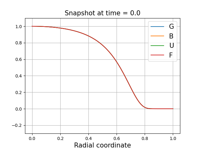
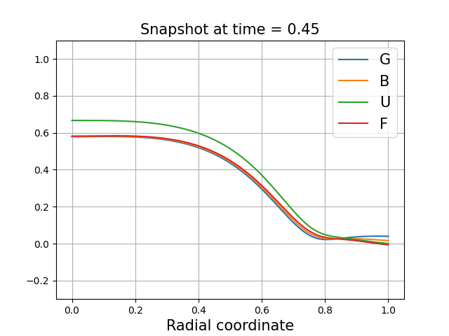
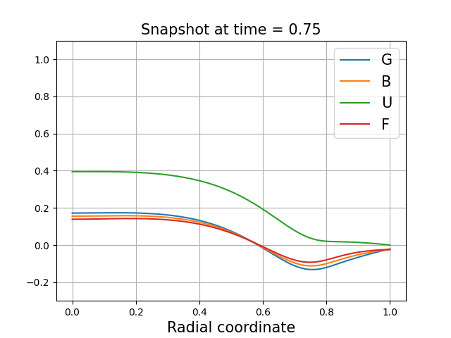
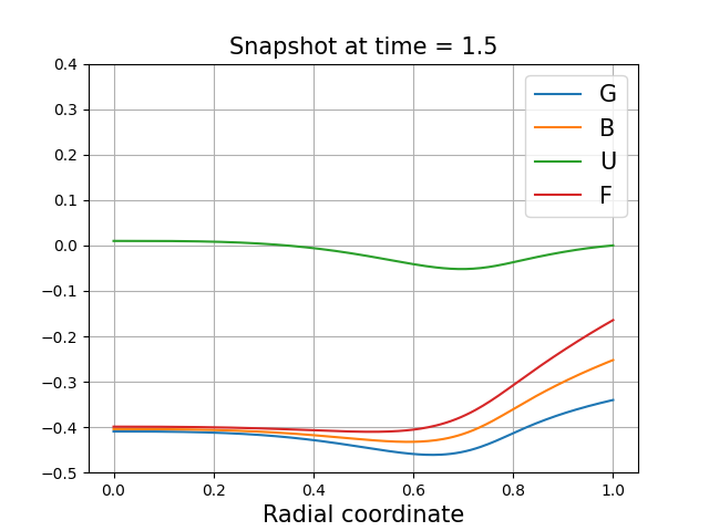
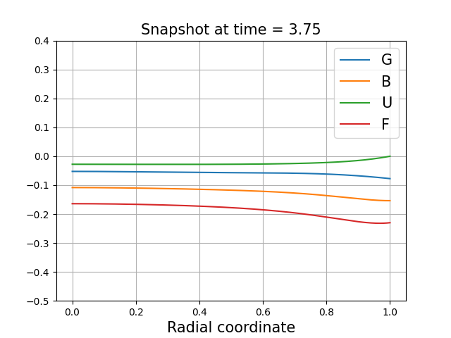
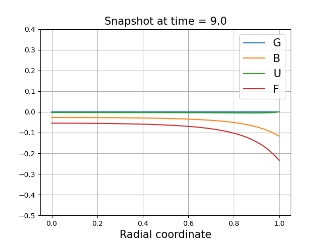
Figure 1: Snapshots of spherically symmetric evolutions. Observe that all the fields reach a stationary state but have different asymptotics. In particular, the good field leaves entirely the domain and the ugly field is zero at $\mathscr{I}^{+}$ for all times.

We have implemented the GBUF model, employing the compactified hyperboloidal coordinates $(t,r,\theta^{A})$ described above, both within a stand-alone code that explicitly assumes spherical symmetry, and within the 3d NRPy+ infrastructure. The code developed from this infrastructure can be obtained at [35]. Both implementations use the method of lines with a fourth-order Runge-Kutta method for time integration. In the spherically symmetric case, the grid has points lying exactly at the origin and at $\mathscr{I}^{+}$, as opposed to the 3d case, in which a staggered grid is used. Spatial derivatives are approximated by second-order accurate centered finite differences, except at infinity, where one-sided derivatives are taken following a truncation error matching approach (see [24]).

In both codes, the interior and outer boundaries require special treatment. The interior boundary corresponds to the boundary of the angular coordinates, in the $3$d case or to the origin $r=0$, in all cases. Ghost points in the $r<0$ case are populated using the parity of the original fields. The original variables $g$, $b$, $u$ and $f$ are even in $R$. In the 3d implementation, angular ghost points are filled with the values of the corresponding gridpoints inside the domain. In the continuum problem, no boundary condition is needed at $r=r_{\mathscr{I}}$, and we find it sufficient to fill the $r>r_{\mathscr{I}}$ ghost points with extrapolation, which we take to be fourth order.

It is well known that the origin is a coordinate singularity in spherical polar coordinates. This fact can be problematic in numerics if the most naive discretizations are used, and turns out to be particularly subtle for first order systems. Because of this, Evans method [32, 36] is used to treat the equations at the origin. To do this, we first use the identity $\frac{R^{\prime}}{R}\Psi=\left(\frac{1}{r}-\frac{\Omega^{\prime}}{\Omega}\right)\Psi$. We then discretize $\partial_{r}\Psi+\frac{2}{r}\Psi$ by

$$\left[\partial_{r}\Psi+\frac{2}{r}\Psi\right]_{j}\approx 3\,\frac{r_{j+1}^{2}\Psi_{j+1}-r_{j-1}^{2}\Psi_{j-1}}{r_{j+1}^{3}-r_{j-1}^{3}}\,.$$

This trick is used to replace all the terms in which $R^{-1}$ appears explicitly as a coefficient of an evolved field.

Finally, we apply artificial dissipation on all variables on the whole grid. For the spherically symmetric runs, this dissipation is just the standard fourth order Kreiss-Oliger dissipation [37] with a dissipation parameter $\sigma=0.02$ using Evans method at the origin, and instead $\sigma=0.01$ with our SBP inspired discretization (described in detail in section III.1). In NRPy+, because of the use of spherical polar coordinates, the dissipation operators are adjusted with $r^{-1}$ and $(r\sin\theta)^{-1}$ factors on the $\theta$ and $\phi$ derivatives, respectively [38, 31]. Nevertheless, in the full 3d case, more dissipation is required to eliminate high frequency errors coming from the origin that eventually make the simulations fail. This noise is likely due to the fact that the coordinate singularity is more severe without symmetry, as it affects all points with $\theta=0,\pi$. In this setting, following [38, 31], we therefore use an overall dissipation factor of around $\sigma=0.4$. By performing evolutions on plain Cauchy slices, we have verified that these modifications are not particular to the use of hyperboloidal coordinates.

As is standard for error analysis in numerical work, we perform norm-convergence tests for both setups. Because of the change of coordinates and the introduction of our slightly non-standard first-order reduction variables, the energy norm associated with the plain scalar field takes the form [24]

$$E(t) =\int\left[\left(\frac{2R^{\prime}-1}{2R^{\prime}\chi^{2}}(\Psi^{+}-\chi^{\prime}\Psi)^{2}\right)+\frac{1}{2R^{\prime}}(\Psi^{-})^{2}\right.$$

$$\qquad\left.+\frac{1}{R^{2}}(\Psi_{\theta}^{2}+\Psi_{\phi}^{2})\right]\frac{R^{\prime}R^{2}}{\chi^{2}}\sin(\theta)drd\theta d\phi\,.$$ (9)

This is the norm used in our numerical convergence tests.

III.1 Spherically symmetric test bed for 3d evolutions

Many interesting features of the model can already be studied in the spherically symmetric case, for which the evolutions are performed with the stand-alone infrastructure used for instance in [18, 23]. We give centered Gaussian ID corresponding to $\psi(t=0,r)\propto e^{-R(r)^{2}}$ and $\partial_{T}\psi(t=0,r)=0$ for all the fields, and define the ID for all the FOR variables accordingly.

One feature of interest is the rate of decay of the fields near null-infinity. Placing certain assumptions on initial data and employing the asymptotic systems approach of [26], specific rates were predicted in [29]. The snapshots in figure 1 show that the evolved fields remain $O(1)$ for all times in accord with these predictions. Since we choose the ID for the ugly fields corresponding to $m_{u}=0$, the ugly fields vanish at $\mathscr{I}^{+}$. The rest of the fields behave asymptotically like the $G$ variables and so oscillate at $\mathscr{I}^{+}$. Interestingly near $\mathscr{I}^{+}$, the $B$ and $F$ fields appear to reach a stationary but non-vanishing state at late (hyperboloidal) times.

It is entirely expected that there is no incoming signal from $\mathscr{I}^{+}$, but it is interesting that this behavior is captured well by the numerical approximation, and furthermore that we see no evidence of incoming waves being generated as reflections in a neighborhood of $\mathscr{I}^{+}$ either. Instead we see the signal practically leaving the domain in finite hyperboloidal time.

Next, we successfully performed long convergence tests on our numerical solutions, examining the data both pointwise and in the energy norm (III). At the base resolution, we took $200$ gridpoints in the radial coordinate, doubling resolution at every level of the convergence test. The energy norm convergence rate, computed on all the fields, is shown as a function of time in figure 2.

Recall that the main objective of this work is to show that the system at hand, viewed as a model for the EFEs in GHG, can be reliably numerically evolved on compactified hyperboloidal slices. We therefore check pointwise convergence for the gridpoints at $\mathscr{I}^{+}$ which, in the spherical case, corresponds to a single gridpoint at each time. Rescaled differences at this point as a function of time are shown in figure 2. Since the three curves lie on top of each other, we get the expected convergence order.

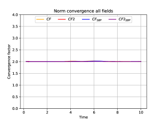
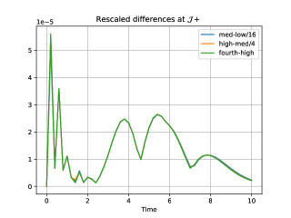
Figure 2: In the left panel we show norm convergence for the entire state vector. Orange and red curves show the convergence factor for standard finite differences with the Evans method for first, second, third and second, third and fourth resolutions respectively. Blue and purple curves show the analogous norm convergence factor for the simulations with our second scheme. The data display robust second order convergence. The right panel shows the sum over all the fields, including the reduction variables, of the absolute value of the rescaled differences at $\mathscr{I}^{+}$ from the Evans discretization. The three curves overlap very well at all times, meaning we get excellent pointwise convergence at $\mathscr{I}^{+}$.

In all of the above spherical runs, we employed the standard Evans method as described above. To demonstrate that our numerical results are not strongly dependent on this particular choice of variables and numerical scheme, we performed spherically symmetric evolutions also using another discretization. This scheme is similar to the SBP discretization derived in [24]. We use a similar (though not identical) discretization as we still do not have an SBP scheme for the linear part of whole GBUF model. The derivation of such a scheme is left for future work. Both the Evans and SBP-like discretization have the property that they stabilize the approximation even in the absence of artificial dissipation, although dissipation does help suppress undesirable error at the origin.

To implement the SBP-like discretization, we define the rescaled fields as

$$\Psi\equiv\chi\psi\,,\,\Psi^{+}\equiv\chi^{2}\psi^{+}\,,\,\Psi^{-}\equiv\chi\psi^{-}\,,$$ (10)

where, as before, $\psi$ is one of the $g$, $b$, $u$ or $f$ variables and $\psi^{+}$ and $\psi^{-}$ are defined in (6). The associated FOR constraints are

$$\frac{\chi}{R^{\prime}}\left(\partial_{r}\Psi+\frac{\Psi^{-}}{2}\right)-\Psi\chi^{\prime}+\left(\frac{1}{2R^{\prime}}-1\right)\Psi^{+}=0\,.$$ (11)

Defining

$$\tilde{\partial}_{r}\Psi\equiv(\chi^{2}R^{-2})\partial_{r}(R^{2}\chi^{-2}\Psi)\,,$$ (12)

the equations take the form

$$\partial_{t}\Psi =\frac{1}{2}\left(\frac{\Psi^{+}}{\chi}+\Psi^{-}\right)\,,$$

$$\partial_{t}\Psi^{+} =\frac{\chi}{2(2R^{\prime}-1)}\left((\partial_{r}+\tilde{\partial}_{r})\left(\chi^{-1}\Psi^{+}\right)+(\partial_{r}-\tilde{\partial}_{r})\Psi^{-}\right)$$

$$-\frac{R^{\prime}}{2R^{\prime}-1}\left(\frac{p\Psi^{+}}{\chi}+(\chi^{\prime}+p)\,\Psi^{-}+S_{\Psi}\right)\,,$$

$$\partial_{t}\Psi^{-}= \frac{1}{2}\Big{(}(\tilde{\partial}_{r}-\partial_{r})\left(\chi^{-1}\Psi^{+}\right)-(\tilde{\partial}_{r}+\partial_{r})\Psi^{-}\Big{)}$$

$$+\frac{R^{\prime}}{\chi}\left(\frac{(\chi^{\prime}-p)\,\Psi^{+}}{\chi}-p\Psi^{-}-S_{\Psi}\right)\,,\,$$ (13)

in the bulk,

$$\partial_{t}\Psi=\Psi^{+}\,,\,\partial_{t}\Psi^{+}=\partial_{t}\Psi^{-}=3\partial_{r}\Psi^{+}-2p\Psi^{+}-S_{\Psi_{0}}\,,$$ (14)

at the origin. Here, the source terms $S_{G}$ and $S_{U}$ are identically zero, and

$$S_{B}= \frac{1}{2}\left(F^{-}+\frac{F^{+}}{\chi}\right)+\frac{1}{4}\left(\frac{G^{+}}{\chi}+G^{-}\right)^{2}\,,$$

$$S_{F}= \frac{1}{2}\left(\frac{G^{+}}{\chi}+G^{-}\right)^{2}\,,$$ (15)

with their limits at the origin being

$$S_{B_{0}}=F^{+}+(G^{+})^{2}\,,\,S_{F_{0}}=2(G^{+})^{2}\,.$$ (16)

The limits at $\mathscr{I}^{+}$ are straightforward. The equations at $\mathscr{I}^{+}$ are obtained by taking the limits

$$U^{-}\rightarrow 0\,,\,F^{-}+\frac{(G^{-})^{2}}{2}\rightarrow 0\,,\,\frac{R^{\prime}U^{-}}{R}\rightarrow-\partial_{r}U^{-}\,,$$

$$\frac{R^{\prime}}{2R}\left(F^{-}+\frac{(G^{-})^{2}}{2}\right)\rightarrow-\partial_{r}F^{-}-G^{-}\partial_{r}G^{-}\,.$$

In our implementation we compute them numerically without using the $\tilde{\partial}_{r}$ operator.

We perform our convergence tests for this discretization in the norm

$$E(t)=\int_{0}^{r_{\mathscr{I}}}\left(\frac{1}{2}r^{2}\Psi^{2}+\varepsilon_{S}\right)\,dr\,,$$ (17)

with

$$\varepsilon_{S}=\frac{1}{2}\left[\frac{(\Psi^{-})^{2}}{2}+\left(\frac{2R^{\prime}-1}{2\chi^{2}}\right)(\Psi^{+})^{2}\right]\frac{R^{2}}{\chi^{2}}\,,$$ (18)

where $\psi$ stands for any of the $g$, $b$, $u$ or $f$ variables, and $\Psi$, $\Psi^{+}$ and $\Psi^{-}$ are defined as in (10). To make the norms in the two discretization schemes compatible with each other, we add $r^{2}\Psi^{2}/2$ to the integrand of the norm (III), when working in spherical symmetry. However, no such modification is introduced in the full $3$d case, and the norm (III) is used. In all cases, the argument in $E(t)$ stands for the hyperboloidal time over which the integral on the right is evaluated.

As can be seen in Figure 2, all the results in the SBP inspired discretization look similar to those obtained using Evans method. The FOR constraint violations in both the schemes also converge perfectly at second order. These violations arise only because of the discretization, as our ID satisfies the reduction constraint in the continuum limit.

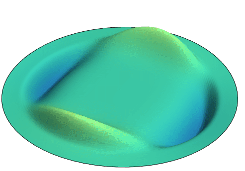
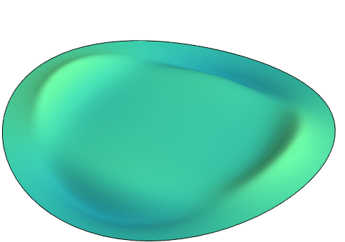
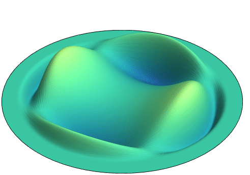
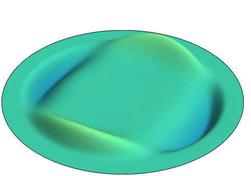
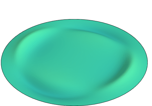
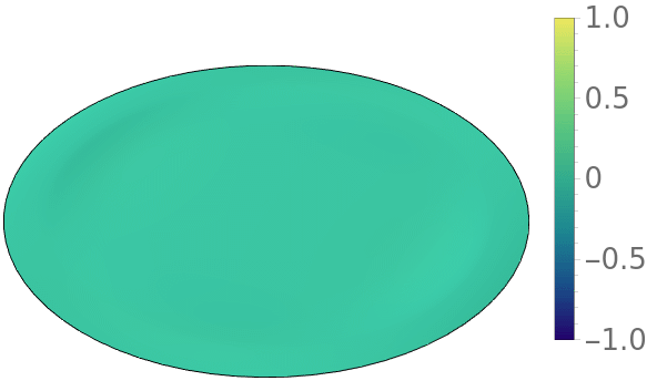
Figure 3: Snapshots of 3d evolutions of B and U fields (on the top and bottom rows) as functions of $r$ and $\phi$ for $\theta\simeq 1$ radian. Observe that similar features can be seen as compared to the spherically symmetric runs, namely, a stationary solutions is reached and the ugly field is zero at $\mathscr{I}^{+}$ for all times. The $G$ and $F$ fields look qualitatively similar.

III.2 Full 3d case

Our next task is to see whether numerical evolutions of the GBUF system can be performed with null-infinity without symmetry assumptions. To this purpose, we perform full 3d evolutions using spherical polar coordinates. Unfortunately, even putting aside the additional computational cost, this is not a completely straightforward generalization of the previous case. The main complication is that we now encounter a “more singular” behavior at the coordinate singularity along the whole $z$ axis. To manage that challenge, besides using Evans method, we follow the basic philosophy of NRPy+, dividing the $\phi$ derivative of the fields by $\sin\theta$ (see 6). The corresponding dissipation operator also needs to be modified as described above. Another strategy to manage these challenges would be to make a multipatch approach, as, for instance, in earlier numerics for the hyperboloidal treatment of the wave equation with the pseudospectral bamps code [39]. Presently, to evolve the full $3$d system numerically, we used NRPy+ [31], a numerical relativity Python infrastructure that outputs optimized C code for the runs. Ideally, this C code is just compiled and run within NRPy+. There were however two places where, in our implementation, the C code was modified directly by hand because the NRPy+Python environment was not designed to automate the particular bespoke changes we required. First were the $r<0$ ghostpoints, which were populated by parity conditions. This is because the $\Psi^{\pm}$ fields evaluated at points $r<0$ involve $\Psi^{\mp}$ and $\Psi$ evaluated at $r>0$. Second was the implementation of Evans method, which was not used (or needed) in the original second order in space NRPy+ implementation of the wave equation on Cauchy slices. All the modified files, including those needed to create the code, together with instructions for compilation and use of the code can be found at the aforementioned link [35].

To avoid directly facing the singular nature of the coordinates, the code uses a staggered grid in the three spatial coordinates, $(r,\theta,\phi)$. This means that the spatial domain in a coordinate, say $r\in(0,1)$, is divided in $N_{r}$ cells, and there’s a gridpoint in the center of each cell. The same is done for the $\theta$ and $\phi$ domains. This is standard in the NRPy+ infrastructure.

As a first test, we input the same ID as in the spherical-code with $(200,4,4)$ gridpoints in the respective $(r,\theta,\phi)$ coordinates at the base resolution. For this case we employed the same dissipation operators and parameters as for the spherically symmetric code, but with full 3d evolution, and made a side-by-side comparison. For the same resolution, the difference in the gridfunctions outputted from the different codes differ at most by numbers of order $O(10^{-3})$, for gridfunctions of order $O(1)$, so they differ by less than $1\%$. Moreover, the largest differences appear close to the origin, and for most of the grid the errors decrease to as little as $O(10^{-7})$. We also performed norm-convergence tests for the spherical code with a staggered grid and the 3d one, by tripling resolution 2 times in the radial coordinate, and compared them directly. Norms calculated from the different codes outputs differ by numbers of order $O(10^{-3})$ for all times, so they differ by less than $1\%$ as well. We take the excellent agreement of the codes in this setup as evidence for the correctness of the 3d implementation.

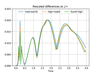
Figure 4: Norm convergence and absolute value of rescaled differences at $\mathscr{I}^{+}$ for the state vector. We observe convincing norm convergence as a function of time with a slight drift for late times. Good pointwise convergence at $\mathscr{I}^{+}$ can also be seen from the figure on the right, even though these curves were calculated by extrapolating the data half a grid point.

For the ID with no symmetry, we use a partial-wave-like expression of the form

$$\psi(t=0) =\frac{A}{4R}e^{-(1+4R)^{2}/16}\big{[}-4-2R-15R^{2}$$

$$\quad+8R^{3}+16R^{4}+e^{R}(4-2R+15R^{2}$$

$$\quad+8R^{3}-16R^{4})\big{]}\,Y_{22}(\theta,\phi)\,,$$ (19)

where $Y_{22}$ is the $l=2,\,m=2$ spherical harmonic and the amplitude parameter $A$ is a constant. This choice was taken because a smooth solution at the origin with no symmetry is needed for this simulation, with the expression inspired by the d’Alembert partial-wave solution to the wave equation for a given smooth function [40, 41], which in this case we take to be $S(R)=R^{2}e^{-(R-\frac{1}{4})^{2}}$. We take the constant $A=1$ for the bad, ugly and $f$ fields and $A=1/10$ for the $g$ field. We choose this because larger values of the $g$ field make it completely dominate the behavior in the $b$ field through the nonlinearity, and we wanted to see evidence of the linear radiation field besides. In figure 3 we show snapshots of the evolution of the system as a function of $r$ and $\phi$ for a particular choice of $\theta$. The same features as in the spherically symmetric case can be seen, namely, the appropriate decay rates and the signal leaving the domain in finite hyperboloidal time, leaving behind a stationary solution.

Norm convergence tests were also performed for the 3d setting, again using the norm in expression (III). We started with $(80,16,32)$ gridpoints in $(r,\theta,\phi)$ coordinates, respectively, and increased resolution by a factor of $1.5$ three times in each coordinate. Fourth-order interpolation was used to match the higher resolution gridpoints to the lowest one’s grid, except at the numerical boundaries, where the third order was used. The result is shown in the left panel of figure 4. Respectable second order convergence is visible in the plot. A slight drift from the ideal convergence rate is seen for late times, although by these times, the data has already mostly left the numerical domain (recall that a purely radially outgoing pulse travelling at the speed of light takes around $t=1$ to reach $r=r_{\mathscr{I}}$ in our coordinates). Second order pointwise convergence at $r=r_{\mathscr{I}}$ is examined in the right hand panel of figure 4, and is similarly promising.

IV Conclusions

In this work, a direct extension of [39, 42, 23, 24], we made another step towards including future null-infinity in generic numerical relativity simulations of asymptotically flat spacetimes. Our strategy is to extend formulations of GR, specifically the GHG system, that are known to work well in the strong-field region on to compactified hyperboloidal slices. One challenge is that, unlike the Conformal Field Equations [11], the resulting system of PDEs may not be regular at null-infinity because, depending on the specific choice of gauge source function, non-principal terms may lack sufficient decay in radius to offset divergences due to the radial compactification. Our direct starting point here was the demonstration provided by [29] that, with care, the gauge source functions can be chosen so that the worst $O(\log(R)/R)$ decay present with a naive choice of the gauge sources is circumvented. Under that approach, the evolved variables have full $O(1/R)$ decay near $\mathscr{I}^{+}$. The subtlety that remains to be handled numerically are formally singular terms. The purpose of this paper was to demonstrate that these terms could be managed numerically both in spherical symmetry and full 3d simulations. Since this difficulty can be made explicit without the full complication of the EFEs, we studied a toy model. We presented numerical evolutions of the Good-Bad-Ugly-F model, a system of nonlinear wave equations that mimics the asymptotic properties of the EFEs in GHG. We showed that the various different fields, each with different decay rates towards $\mathscr{I}^{+}$, can be evolved numerically on compactified hyperboloids.

In related earlier work [39] pseudospectral numerics for the wave equation on hyperboloidal slices was presented. Here instead, because of the potentially slow asymptotic decay of fields in the GBUF model, purely as a proof-of-principle, we employed finite differences exclusively for the approximation of spatial derivatives. We made two numerical implementations, one in explicit spherical symmetry (with two distinct choices of variables and discretization), the other in 3d using NRPy+. Our first important result was that the decay rates for each of the fields predicted in [29] were reliably obtained in both codes, and for all of the initial data sets we treated. Moreover, the expected properties of hyperboloidal evolution of wave-like equations with our setting were observed. Among these were the finite but non-vanishing velocities of the signals going through $\mathscr{I}^{+}$ and, for a subset of the fields, the presence of non-vanishing near-stationary solutions after a finite hyperboloidal time. Clean norm convergence and pointwise convergence at $\mathscr{I}^{+}$ is seen for all cases from our numerics. In summary: the results presented here show that there should be no problem in managing the asymptotic properties of the EFEs in GHG on compactified hyperboloidal slices.

An interesting point that we have made no attempt whatsoever to understand here is the effect of choosing initial data that decay only very slowly towards $\mathscr{I}^{+}$. This would make direct contact with [43], where such initial data were considered for a subsector of the GBUF model. In the context of GR, such data has relevance to the question of the peeling property at $\mathscr{I}^{+}$ (see [44, 45, 46, 47] for recent work in this direction). Unfortunately, treating such initial data would force a complete rethink of the numerical strategy.

Many pieces of the puzzle are now in place for a $3+1$ implementation of the EFEs on hyperboloidal slices. There are a number of outstanding questions however, including for instance our incomplete understanding of charges at $\mathscr{I}^{+}$ expressed in generic generalized harmonic gauges, the lack of a clear (stand-alone) local well-posedness theory on hyperboloidal slices and the hands-on construction of initial data for a variety of scenarios of interest. Progress on all these fronts is expected. In the near-term we will present a comprehensive set of spherical numerics for full GR.