Metastate analysis of the ground states of two-dimensional Ising spin glasses

Abstract

Using an efficient polynomial-time ground state algorithm we investigate the Ising spin glass state at zero temperature in two dimensions. For large sizes, we show that the spin state in a central region is independent of the interactions far away, indicating a “single-state” picture, presumably the droplet model. Surprisingly, a single power law describes corrections to this result down to the smallest sizes studied.

I Introduction

Spin glasses are prototypical disordered models Binder and Young (1986); Mézard et al. (1987); Fischer and Hertz (1991); Young (1998) studied in statistical mechanics, with applications in various fields such as machine learning, neural networks, and optimization Nishimori (2001); Hartmann and Weigt (2005); Mézard and Montanari (2009); Moore and Mertens (2011); Kawashima and Rieger (2013). Despite considerable effort, the nature of the spin glass state in three dimensions below the transition temperature $T_{c}$ remains uncertain. In equilibrium it is not possible to study very large sizes numerically because relaxation is very slow in Monte Carlo Newman and Barkema (1999) simulations, and because a large number of samples have to averaged over. Because we don’t know how large are corrections to the asymptotic scaling behavior, it is difficult to judge whether results obtained in numerics show the asymptotic behavior or just a pre-asymptotic crossover.

The two main scenarios which have been proposed for the nature of the spin glass state are the droplet picture Fisher and Huse (1986, 1988); McMillan (1984a); Bray and Moore (1986) and the replica symmetry breaking (RSB) Parisi (1979, 1980, 1983) picture. An important distinction between these two approaches is that the droplet theory is a one-state picture, and RSB is a many-state picture. To explain what this means we have to note that the state of the system can possibly depend chaotically on system size. Because of this, to describe spin glasses we need the “metastate” proposed by Newman and Stein (NS) Newman and Stein (1997, 2006) and by Aizenmann and Wehr (AW) Aizenman and Wehr (1990). These two versions of the metastate are generally thought to be equivalent but the AW metastate is more convenient for our purposes so we will consider that here. For more information on the metastate in spin glasses see e.g. Ref. Read (2014).

The basic idea of the metastate is to measure how some part of the system, expressed in terms of correlations, depends on changes in other parts of the system. Ideas related to the metastate can be found in other works, were distribution of window overlaps or probabilities of subsystem configuration changes induced by changes of the boundary conditions were investigated for spin glasses Palassini and Young (1999); Manssen et al. (2015); Middleton (1999), random-field systems Middleton and Fisher (2002) and others Middleton (1999). To construct the AW metastate, take a large system of linear size $L$ and divide it into an inner region of size $M\ (<L)$ and an outer region. Determine the state of the system, and record the spin correlations in a small central region of size $K\ (\ll M)$ in the middle of the inner region. This is illustrated in Fig. 1 for $L=8,M=4,K=2$. Then change the bonds in the outer region only and recompute the correlations in the small central region. Repeat this many times and, for $M,L\to\infty$, see if the central correlations are independent of the outer bonds, which corresponds to a one-state picture, or whether they change as the outer bonds are changed, which corresponds to a many-state picture.

At least in zero magnetic field, numerics in three dimensions seems to favor a many-state picture, see e.g. Billoire et al. (2017), but supporters of the droplet picture suggest that there are large corrections to scaling for the sizes which can be reached, and the observed behavior is just a crossover.

The above is for three dimensions. However, in two dimensions the situation is different for two reasons. Firstly there is overwhelming evidence that the transition only occurs at zero temperature McMillan (1984b); Bray and Moore (1984); Rieger et al. (1996); Hartmann and Young (2001), and secondly there are highly efficient polynomial-time algorithms for computing the ground state Bieche et al. (1980); Hartmann and Rieger (2001); Hartmann (2007); Thomas and Middleton (2007); Pardella and Liers (2008) at least if there are periodic boundary conditions in no more than one direction. It is generally accepted, though not rigorously proved except for a half-plane Arguin et al. (2010), that the droplet picture (a one-state picture) applies in two dimensions and more generally when the transition is at $T=0$. Although there was some confusion in the past due to an exponent relating energy to size being apparently different for “domain wall” and “droplet” excitations, which would contradict the droplet theory, it was later shown by one of us and Moore Hartmann and Moore (2003, 2004) that this apparent difference is due to corrections to scaling being large for droplet excitations (though small for domain walls), and for large enough sizes the exponents are the same.

In this paper we use efficient ground state methods for a large range of sizes to directly address the one-state versus many-state issue in two dimensions by investigating the AW metastate at $T=0$. We find a one-state picture, i.e. consistent with the droplet theory, since, in the limit of large system size, correlations at the center don’t depend on the bonds far away. Of particular interest is whether there are large corrections to scaling which could prevent this result being deduced from small sizes only. In fact there are not. The extrapolation to infinite size follows a single power law down to very small sizes. This is in contrast to certain other quantities for which large sizes are needed to observe the true scaling behavior Hartmann and Moore (2003, 2004).

The plan of this paper is as follows. In Sec. II we define the model and the quantities we calculate. Our results are described in Sec. III and our conclusions summarized in Sec. IV.

II The Method

We use the standard Edwards-Anderson Edwards and Anderson (1975) of the Ising spin glass in zero field, for which the Hamiltonian is given by

$$\mathcal{H}=-\sum_{\langle ij}J_{ij}S_{i}S_{j}\,,$$ (1)

where the nearest-neighbor interactions $J_{ij}$ are independent Gaussian random variables with zero mean and standard deviation $1$, and the $S_{i}$, which take values $\pm 1$, lie at the sites of a square lattice of size $L\times L$. We work at $T=0$. Because the bond distribution is continuous, the ground state is unique, apart from inversion of all the spins as discussed in footnote 1.

We use a fast polynomial-time algorithm Bieche et al. (1980); Hartmann and Rieger (2001); Hartmann (2007) for which periodic boundary conditions can be applied at most in one direction. In order to preserve the symmetry of the square lattice we take free boundary conditions in both directions.

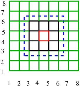
Figure 1: (color online) The setup for size $L=8$. The boundary between the interior and exterior regions is indicated by the dashed blue line. For all sizes $L$, the inner region is of size $M=L/2$, so $M=4$ here. Also, for all sizes we just measure the spin correlations in the central square (size $K=2$), which is shown in red. The rest of the interior region is shown in black. The exterior region, whose bonds are changed after each run, is in green. Note that we take free boundary conditions.

The setup is shown in Fig. 1 for $L=8$ (we need $L$ to be a multiple of $4$). The lattice is divided into “inner” and “outer” regions separated by the (blue) dashed line in the figure. For all lattice sizes $L$ the inner region is of size $M=L/2$, so if we label a site by $(x,y)$ where $x$ and $y$ take values $1,2,\cdots,L$, then the values of $x$ and $y$ for sites in the inner region have $x$ and $y$ in the range $L/4+1$ to $3L/4$. After determining the ground state we record the four nearest-neighbor spin correlations for the spins on the central square (colored red in the figure) for which the $x$ and $y$ values are $L/2$ and $L/2+1$.

Note that we fix the ratio $M/L$ to be $1/2$ as $L$ increases but the region where we compute the spin correlations is always just the central square (so the size is $K=2$). Hence we consider the limit where $L/K$ and $M/K$ become large with $L/M$ fixed.

Having recorded the spin orientations in the central square for a particular choice of the bonds we then change the bonds in the outer region only (shaded in green in Fig. 1) and recompute the ground state. This leads to strong changes of the configuration in the outer region, basically half of the spins, and some changes in the inner region, where the bonds have not changed. Two examples for the difference between such pairs of ground states are shown in Fig. 2. The ground states in the inner region typically differ only by small spin clusters or by one large cluster, respectively.

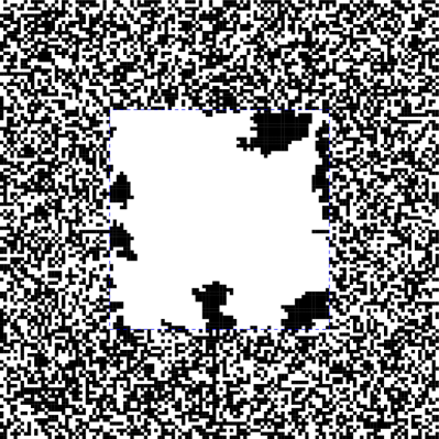
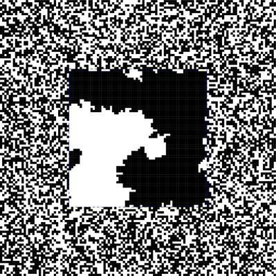
Figure 2: Comparison between pairs of ground states for $L=128$ which differ by changes of the bonds in the outer region. Black squares indicate spins which a different. The left figure shows an example where few small clusters in the inner region are flipped, while the right figure shows a flip of mainly one big cluster.

We repeat for many sets of outer bonds but the same inner bonds and denote the corresponding average by $[\ldots]_{\mathrm{out}}$. For $i$ and $j$ nearest-neighbor sites on the central square we compute the average

$$C_{ij}^{\mathrm{meta}}=\Bigl{|}\,[S_{i}S_{j}]_{\mathrm{out}}\Bigr{|},$$ (2)

which is known as a “metastate” average. Here we take the modulus to get rid of the random sign. Normally in spin glasses one takes the square, but there is a reason discussed in connection with Fig. 4 why we prefer to take the modulus here. Almost identical results for the intercept $a$ and exponent $\lambda$ in Eq. (5) below are obtained if we use the square rather than the modulus. Note that the modulus is performed only after the average over the outer bonds is done. For each configuration of both inner and outer bonds $S_{i}S_{j}=\pm 1$ since the ground state is unique apart from spin inversion. Thus, if the state in the central region is completely independent of the outer bonds one has $C_{ij}^{\mathrm{meta}}=1$. However, if the state in the central region depends on the outer bonds one has $C_{ij}^{\mathrm{meta}}<1$.

Next we average over the inner bonds to get

$$C_{\mathrm{meta,av}}=[\,C_{ij}^{\mathrm{meta}}\,]_{\mathrm{in}}=[\,\Bigl{|}\,[S_{i}S_{j}\,]_{\mathrm{out}}\,\Bigr{|}\,]_{\mathrm{in}}\,.$$ (3)

To get the best statistics we also average over the four nearest neighbor pairs in the central square in Fig. 1.

According to a one-state picture

$$C_{\mathrm{meta,av}}\to 1\ \mathrm{for}\ L\to\infty\quad\mathrm{(droplet\ theory)},$$ (4)

while in a many-state picture, $C_{\mathrm{meta,av}}$ tends to a value less than $1$ in this limit.

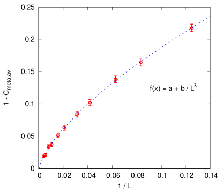
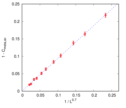
Figure 3: (color online) The upper panel plots $1-C_{\mathrm{meta,av}}$ against $1/L$ for different sizes as well as a best fit according to Eq. (5). The fit parameters are $a=-0.004\pm 0.005,\lambda=0.66\pm 0.05,b=0.89\pm 0.08$. The lower hand panel plots the same data against $1/L^{0.7}$. This power is chosen because the best fit with $a$ fixed to be $0$ gives $c=0.70\pm 0.02$.

III Results

We have performed computations for sizes, $L=8$ to $L=256$ using an efficient polynomial time algorithm Bieche et al. (1980); Hartmann and Rieger (2001); Hartmann (2007) For each size we average over 100 choices of the outer bonds for a given choice of the inner bonds. This procedure is then repeated for 1000 values of the inner bonds so altogether we do $10^{5}$ ground state computations for each size.

The upper panel of Fig. 3 plots $1-C_{\mathrm{meta,av}}$ against $1/L$. To compute the error bars, we first average over the four nearest neighbor pairs in the central square, to get a single number for each sample. Since different samples have statistically independent values for both the inner and outer bonds, the results for different samples are statistically independent and so error bars can be computed in the standard way from these results. Also shown is a fit to the function

$$1-C_{\mathrm{meta,av}}=a+{b\over L^{\lambda}},$$ (5)

which gives

$$a =-0.004\pm 0.005$$ (6)

$$b =0.89\pm 0.08$$ (7)

$$\lambda =0.66\pm 0.05\,.$$ (8)

The quality of this fit is $Q=0.99$, very close to $1$, which is a bit surprising. This may, partly, be a statistical coincidence, and partly due to the values of $C_{ij}^{\mathrm{meta}}$ not being Gaussian distributed (as can be inferred from Fig. 4), so the true fit probability can not be obtained directly from the $\chi^{2}$ per degree of freedom.

Our main result is that the extrapolated value $a$ is zero to within very small error bars which provides evidence that $C_{\mathrm{meta,av}}\to 1$ for $L\to\infty$ indicating a one-state picture.

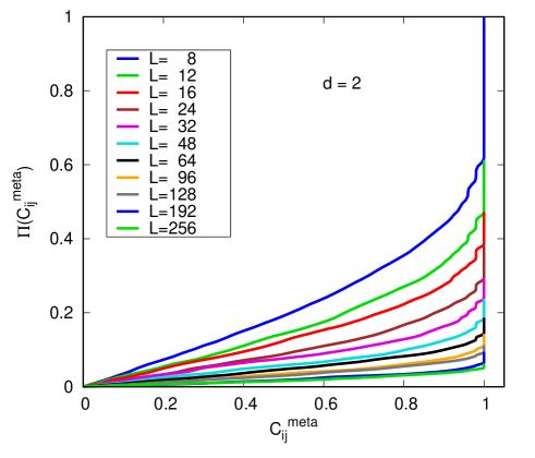
Figure 4: (color online) The cumulative probability distribution of $C^{\mathrm{meta}}_{ij}$ is plotted for different sizes. If $P(C^{\mathrm{meta}}_{ij})$ is the probability distribution of $C^{\mathrm{meta}}_{ij}$ averaged over both the inner bonds and the four central nearest-neighbor pairs shown in Fig. 1, then the cumulative distribution $\Pi(y)$ is defined by $\Pi(y)=\int_{0}^{y}P(x)\,dx.$ The order of the lines in the figure is the same as in the legend. The distribution is actually discrete; the only values of $C_{ij}^{\mathrm{meta}}$ which can occur are $0,0.02,0.04,\cdots,1.00$ since we take 100 sets of outer bonds for each set of inner bonds, and $S_{i}S_{j}$ can only take the values $\pm 1$ at $T=0$. Note that the allowed values of $C_{ij}^{\mathrm{meta}}$ are uniformly spaced. This is because we defined $C_{ij}^{\mathrm{meta}}$ in Eq. (2) with a modulus. However, if we had defined it with a square instead, which would usually be more natural for spin glasses, the allowed values of $C_{ij}^{\mathrm{meta}}$ would not be uniform.

If we fix $a=0$, a fit gives $\lambda=0.70\pm 0.02$ with the same quality $Q=0.99$ of the fit. The lower panel in Fig. 3 plots $1-C_{\mathrm{meta,av}}$ against $1/L^{0.7}$. It is remarkable than an excellent straight-line fit is obtained for all sizes from $L=8$ upwards. Hence single-state behavior could be deduced even for small sizes. However, one would not be confident that this is the correct behavior without also having the results for large sizes.

Note that the changes in the inner region are composed of clusters seperated by domain walls, see Fig. 2. Thus, the value of the exponent $\lambda$ is likely related Palassini and Young (1999); Middleton (1999); Middleton and Fisher (2002) to the fractal nature of the domain walls . The domain-wall lengths $l$ scale as $L^{d_{\textrm{f}}}$ where $d_{\textrm{f}}$ is the fractal dimension. Since the number of affected bonds scales as $l$, the probability that a bond from the $O(L^{2})$ bonds in the inner region is affected should scale as $L^{2}/L^{d_{\textrm{f}}}=L^{2-d_{\textrm{f}}}$, i.e., $\lambda=2-d_{\textrm{f}}$. With estimates of $d_{\textrm{f}}=1.274(2)$ Melchert and Hartmann (2007) and $d_{\textrm{f}}=1.27319(9)$ Khoshbakht and Weigel (2018) one has $\lambda\approx 0.73$ which compares well with our value $\lambda=0.70\pm 0.02$ quoted above.

To get a more detailed picture, Fig. 4 plots $\Pi(C_{ij}^{\mathrm{meta}})$, the cumulative distribution of $C_{ij}^{\mathrm{meta}}$, defined in Eq. (2), averaged over the different sets of inner bonds and the four central nearest-neighbor pairs in Fig. 1. We see that for a substantial fraction of the choices of the inner bonds one has $C_{ij}^{\mathrm{meta}}=1$. This fraction increases with increasing size and apparently tends to 1 for $L\to\infty$. For these samples there is strictly no change in the relative spin orientation of a central nearest-neighbor pair when the outer bonds are changed. Note that the probability distribution of $C_{ij}^{\mathrm{meta}}$, inferred from the cumulative distribution shown in Fig. 4, is very far from Gaussian, as discussed above in connection with with $Q$-factor of the fits in Fig. 3.

IV Conclusions

We have confirmed the single-state picture for the $T=0$ spin glass state in $d=2$ by using powerful numerical techniques which permit a study of large system sizes. We have shown directly that, at $T=0$ and for $d=2$, the spin glass state in a region only depends the bonds in the vicinity of that region and not on the bonds far away.

An important result is that extrapolation to infinite system size is very smooth. A single inverse power of $L$ describes the decay of $1-C_{\mathrm{meta,av}}$ to zero down to the smallest size studied $L=8$, see Fig. 3. Our estimates for this power, $\lambda$, are $0.66\pm 0.05$ in an unconstrained fit, and $0.70\pm 0.02$ if the extrapolated value is fixed to zero.

The smooth trend with size shown in Fig. 3 down to the smallest size $L=8$ is reminiscent of the domain wall energy. In early work, using sizes only up to $L=12$, Bray and MooreBray and Moore (1984) found the stiffness exponent for the size dependence of domain wall excitations to be $\theta=-0.294\pm 0.009$. Remarkably, this is very close to recent resultsKhoshbakht and Weigel (2018) using efficient methods Bieche et al. (1980); Hartmann and Rieger (2001); Hartmann (2007); Thomas and Middleton (2007); Pardella and Liers (2008) which included sizes between $L=8$ and $10,000$ and which found $\theta=-0.2793\pm 0.0003$. However the situation for the energetics of droplet excitations is different, since for these one needs quite large sizes to see the asymptotic behavior Hartmann and Moore (2003). The reason for this difference is unclear. Unfortunately, it is also unclear what sizes are needed in three dimensions to determine the nature of the spin glass state on large length scales. Furthermore, the situation in three dimensions is more complicated because, in addition to the droplet and RSB pictures, there are additional possibilities such as like the “trivial-non-trivial” and “chaotic-pair” pictures Newman and Stein (2003).