Wasserstein Adversarial Examples on Univariant Time Series Data

Abstract.

Adversarial examples are crafted by adding indistinguishable perturbations to normal examples in order to fool a well-trained deep learning model to misclassify. In the context of computer vision, this notion of indistinguishability is typically bounded by $L_{\infty}$ or other norms. However, these norms are not appropriate for measuring indistinguishiability for time series data. In this work, we propose adversarial examples in the Wasserstein space for time series data for the first time and utilize Wasserstein distance to bound the perturbation between normal examples and adversarial examples. We introduce Wasserstein projected gradient descent (WPGD), an adversarial attack method for perturbing univariant time series data. We leverage the closed-form solution of Wasserstein distance in the 1D space to calculate the projection step of WPGD efficiently with the gradient descent method. We further propose a two-step projection so that the search of adversarial examples in the Wasserstein space is guided and constrained by Euclidean norms to yield more effective and imperceptible perturbations. We empirically evaluate the proposed attack on several time series datasets in the healthcare domain. Extensive results demonstrate that the Wasserstein attack is powerful and can successfully attack most of the target classifiers with a high attack success rate. To better study the nature of Wasserstein adversarial example, we evaluate a strong defense mechanism named Wasserstein smoothing for potential certified robustness defense. Although the defense can achieve some accuracy gain, it still has limitations in many cases and leaves space for developing a stronger certified robustness method to Wasserstein adversarial examples on univariant time series data.

1. Introduction

Deep learning has been widely applied to real-world time series classification tasks including healthcare, power consumption monitoring, as well as social safety and security (Ismail Fawaz et al., 2019b; Tobiyama et al., 2016; Ma et al., 2018). Univariant time series modeling is a common class of applications that deals with one observed variable over time (Karim et al., 2019). The data are often collected from a sensor, such as Electrocardiography (ECG) to measure patient’s heart rhythms (Castells et al., 2007), and can be used for diagnosis and monitoring. Deep learning systems have achieved state-of-the-art performance in most of these tasks.

Figure 1. An example to illustrate the differences between Wasserstein distance and Euclidean distance. The two ECG signals in the upper figure are close in the Wasserstein distance and similar to human perception while they have a large $L_{1}$ distance. In the bottom figure, the $L_{\infty}$ distance from the red curve to the blue and purple curve are both 2.88, but from human perception, the purple curve is much further away from the red curve than the blue curve. Therefore, the Wasserstein distance is more appropriate to measure the distance in this case.

However, recent studies have shown that adversarial examples can be generated to force a well-trained deep learning model to misclassify by applying small and unnoticeable perturbations to the input data (Szegedy et al., 2013). The existence of such adversarial examples reveals the vulnerability of deep learning models, especially when applied to security-critical domains such as healthcare.

The notion of indistinguishability of adversarial examples, in the context of computer vision, was originally taken to be $L_{\infty}$ bounded perturbations, which refers to noise with limited magnitude injected to each pixel (Goodfellow et al., 2014). Followed by that, the scale of adversarial perturbations is usually constrained by $L_{p}$ norm, i.e., bounded by an $L_{p}$ norm ball centered at the normal example (Kurakin et al., 2018; Carlini and Wagner, 2017). As deep learning models are increasingly used for time series data, several works adapted adversarial attacks from images to time series data (Ismail Fawaz et al., 2019a; Karim et al., 2021; Mode and Hoque, 2020) using $L_{p}$ norms. While adversarial examples under $L_{p}$ norm are intuitive for image classification tasks, $L_{p}$ norm is not an appropriate metric for the time series data.

In time series analysis, there are more effective metrics for measuring similarity between two temporal sequences, especially when the sequences vary in length and speed (Alt and Godau, 1995; Berndt and Clifford, 1994). Wasserstein distance (Vallender, 1974), which is the numerical cost of an optimal transportation problem, allows us to analyze the distance between two time sequences. This distance can be intuitively understood for time sequence as the cost of moving around feature mass from one time step to another (transportation plan) in order to make two sequences the same.

Note that Wasserstein distance and Euclidean distance are different measures and even opposite in some cases. Two time sequences can be close in the Wasserstein distance while far away from each other in Euclidean distance. As shown in Figure 1, Wasserstein distance can better reflect human perception. The time series that appear more distinguished to our eyes are captured by larger Wasserstein distances. The example in the upper figure may not be a successful adversarial example under $L_{1}$ distance as it is distant in the $L_{1}$ space. However, it is almost imperceptible to human evaluation. In this case, Wasserstein distance is a better measurement of adversarial examples.

In this work, we study the adversarial attack on time series in the Wasserstein space for the first time. Our goal is to generate adversarial examples that have small Wasserstein perturbation so it is more indistinguishable and natural to human, e.g., physician who examines ECG data. Projected gradient descent attack (Madry et al., 2017) is a widely-used attack method that applies small steps of maximizing the loss objective iteratively and clipping the values of intermediate results after each step (projection to the $L_{p}$ norm ball) to ensure that they are in a constrained neighbourhood of the original inputs. Similarly, we propose a Wasserstein PGD method to search for adversarial examples in the Wasserstein space for univariant time series. Wasserstein distance cannot be calculated directly without solving an optimization subproblem and has no closed-form solution in most cases, which limits its applications. At present, there are only two cases that the Wasserstein distance can be directly calculated, one is the case of the dimension of inputs being 1, and the other is the inputs following Gaussian distribution. For the univariant time series, we can take advantage of its $1D$ characteristic and use the closed-form Wasserstein distance to apply the projection of intermediate results of each step onto the Wasserstein ball with gradient descent method.

Figure 2. Illustration of the difference between direct projection and two-step projection

The direct projection of intermediate results onto the Wasserstein ball using gradient descent could be time-consuming and converge to a sub-optimal solution. Thus, we further propose a two-step projection method that first projects the intermediate result to an $L_{p}$ norm ball (one step clipping) and then uses the projected example on the norm ball as the starting point for Wasserstein projection, so that the search in the Wasserstein space is guided and constrained. The intuition of the two-step projection is illustrated in Figure 2, which will be explained in detail in the Method Section.

The state-of-the-art defense mechanism to adversarial examples is the certified robustness approach which provides a theoretical guarantee that adversarial examples generated within certain distance bounds can be correctly classified. To better study the nature of Wasserstein adversarial examples, we also investigate how well the existing certified robustness approach work against our proposed Wasserstein attack. As Wasserstein adversarial examples are bounded by Wasserstein distance, the existing and well-known certified defense within Euclidean distance is not applicable (Cohen et al., 2019). We adapt Wasserstein Smoothing (Levine and Feizi, 2020), a certified robustness approach to Wasserstein adversarial examples for image data which transfers Wasserstein distance on the image into $L_{1}$ distance on the transport plan, to univariant time series adversarial examples. From the results, although the defense can achieve some accuracy gain, it still has limitations in many cases and leaves space for developing a stronger certified robustness method to Wasserstein adversarial examples on univariant time series data.

Our Contributions can be summarized as follows:

1) We study adversarial examples in the Wasserstein space for time series data for the first time which better capture the distance and are more natural and imperceptible.

2) We utilize the characteristics of univariant time series data and propose a projected gradient descent attack method which efficiently projects (bounds) adversarial examples in the Wasserstein ball.

3) We develop a two-step projection that first projects an adversarial example to an $L_{p}$ norm ball and then use the projected example as the starting point for Wasserstein projection to overcome the computing bottleneck of direct Wasserstein projection.

4) We empirically evaluate the proposed attack on several Electrocardiogram (ECG) datasets in the health care domain. Extensive results demonstrate that the Wasserstein PGD is powerful and can attack most of the target classifiers with a high attack success rate and yield more imperceptible and natural examples than attacks in the Euclidean space.

5) We evaluate Wasserstein smoothing designed for image data as a baseline certified robustness approach against Wasserstein attack which suggest that there is space for stronger defense mechanisms tailored to time series data.

2. Related Work

In this section, we will first introduce existing adversarial attacks in the image domain and time series domain. Followed by that we will discuss the state-of-the-art defense mechanism: certified robustness.

2.1. Adversarial Attack Methods

Adversarial examples were first introduced in the image domain (Szegedy et al., 2013). Ian Goodfellow et al (Goodfellow et al., 2014) proposed a fast Gradient Method to generate adversarial examples by performing a one-step gradient update along the direction of the sign of the gradient at each pixel. This method is simple and fast but cannot minimize perturbation. Other research attempted to iteratively apply FGSM in order to achieve a smaller perturbation such as I-FGSM and Projected Gradient Descent (PGD) (Madry et al., 2017; Kurakin et al., 2016). C&W (Carlini and Wagner, 2017) is a powerful attack that aims to both minimize the distance and maximizes classification loss and hence achieves minimal perturbations for the same attack success rate. However, C&W is relatively time-consuming.

The above mentioned attack methods are all in the Euclidean space. (Wong et al., 2019) opened up a new direction in adversarial examples in Wasserstein space for the image domain, by developing a procedure for projecting an example onto the Wasserstein ball. As the projection cannot be directed calculated, they used Projected Sinkhorn Iterations to approximate the projection.

Several works have adapted adversarial attacks from images to time series data. (Ismail Fawaz et al., 2019a) empirically studies the performance of I-FGSM in the time series classification tasks while (Mode and Hoque, 2020) adopted I-FGSM into the time series regression tasks. (Karim et al., 2021) utilized an adversarial transformation network (ATN) (Baluja and Fischer, 2017) on a distilled model to attack various time series classification models. Although Wasserstein distance is a better distance measurement for time series data, no previous work has studied adversarial examples in Wasserstein space for time series data.

2.2. Certified Robustness

Certified robustness is the most powerful defense method to date as it is provable. The main idea is to transform the base classifier into a randomized classifier by applying random noise onto the inputs or classifier, such that the perturbed examples within a certain Euclidean ball are certified to have the same classification as the original example. PixelDP(Lecuyer et al., 2019) utilized the definition of differential privacy (DP) (McSherry and Talwar, 2007) to prove certified robustness using the Gaussian mechanism through noisy layers in the network. WordDP (Wang et al., 2021) extended the idea into the text domain using the Exponential mechanism. Randomized smoothing (Cohen et al., 2019) generates Gaussian noise on the input and provided a tighter certified bound using the Neyman Pearson lemma(Neyman and Pearson, 1992).

Wasserstein smoothing (Levine and Feizi, 2020) was the first certified robustness method for adversarial images in Wasserstein space. The basic idea is to define a reduced transport plan and transfer Wasserstein distance on the image space to $L_{1}$ norm on the transport plan. Therefore, smoothing in the transport domain can be performed using existing $L_{1}$ robustness certification provided by (Lecuyer et al., 2019) and transferred back to the Wasserstein space. In this paper, we will adopt Wasserstein smoothing from the image domain to the univariant time series data and evaluate the performance of our proposed Wasserstein attack against this potential countermeasure.

3. Methods

In this section, we present our proposed Wasserstein adversarial example against time series models. We rely on the most common method of creating adversarial examples, the variation of projected gradient descent (PGD). The original PGD algorithm uses $L_{\infty}$ clipping to perform the projection while we will use Wasserstein projection in our method. First, we will explain how to perform the Wasserstein projection. Followed by that, we will explain the Wasserstein PGD algorithm and the two-step projection.

3.1. Wasserstein Projection

Let $(x,y)$ be a data point and its label, and $\mathcal{B}(x,\epsilon)$ be a ball around $x$ with radius $\epsilon$. The (general) projection of a point $w$ on to $\mathcal{B}(x,\epsilon)$ can be formulated as:

(1) $$\underset{\mathcal{B}(x,\epsilon)}{proj(w)}=\underset{z\in\mathcal{B}(x,\epsilon)}{\mathop{\rm argmin}}||w-z||_{2}^{2}.$$

A Wasserstein ball around sample $x$ with radius $\epsilon$ can be defined as:

(2) $$\mathcal{B}_{w}(x,\epsilon)=\{x+\delta:d_{\mathcal{W}}(x,x+\delta)\leq\epsilon\},$$

where $d_{\mathcal{W}}(u,v)$ refers to the Wasserstein distance between two sample distributions in the space $\mathcal{X}=\mathbb{R}^{2}$, which can be calculated as:

(3) $$d_{\mathcal{W}}(u,v)=[\underset{\gamma\in\Pi(u,v)}{inf}\int_{\mathcal{X}^{2}}||x-y||^{p}d\gamma(x,y)]^{1/p}.$$

Here $\gamma$ defines the joint probability distribution, called coupling, which has marginal distribution exactly as $u$ and $v$.

Input :  Original input: $x$; Initial adversarial input $x_{adv}^{0}$; Wasserstein projection bound: $\mathcal{C}$; Step size: $\alpha$

Output :  Projected Adversarial example: $x_{adv}$

1 $i\leftarrow 0$;

2 $L_{w}^{0}=d_{\mathcal{W}}(x,x_{adv}^{0})$ (Formula 5);

3 while $L_{w}\geq\mathcal{C}$ do

4       $x_{adv}^{i+1}=x_{adv}^{i}-\alpha\cdot\frac{\partial L_{w}(x,x_{adv}^{i})}{\partial x_{adv}^{i}}$;

5       $L_{w}^{i}=d_{\mathcal{W}}(x,x_{adv}^{i})$;

6       i++;

7       if $i\geq\mathbb{I}$ then

8             Break;

9             Return False;

10            

11      

Algorithm 1 1D_Wasserstein_Projection

When the input distribution satisfies the dimension being one, there is a closed-form solution for the above $d_{\mathcal{W}}$:

(4) $$\begin{split}d_{\mathcal{W}}(u,v)&=||F_{u}^{-1}-F_{v}^{-1}||^{p}\\ &=(\int_{0}^{1}||F_{u}(\alpha)^{-1}-F_{v}(\alpha)^{-1}||^{p}d\alpha)^{1/p}.\end{split}$$

When $p$ equals 1 and the inputs are in the discrete case, formula 4 can be further simplified as:

(5) $$\begin{split}d_{\mathcal{W}}(u,v)&=\int_{\mathbb{R}}|F_{u}(\alpha)-F_{v}(\alpha)|d\alpha\\ &=\sum_{i=1}^{n}|\sum_{j=1}^{i}u_{i}-\sum_{j=1}^{i}v_{i}|.\end{split}$$

In this case, the transport plan is $t=F_{v}^{-1}\odot F_{u}$.

Specifically, projecting $w$ onto the Wasserstein ball around $x$ with radius $\epsilon$ is defined as:

(6) $$\underset{\mathcal{B_{\mathcal{W}}}(x,\epsilon)}{proj(w)}=\underset{z\in\mathcal{B}_{\mathcal{W}}(x,\epsilon)}{\mathop{\rm argmin}}d_{\mathcal{W}}(x,z).$$

As $1D$ Wasserstein distance has a closed-form solution and the above formula is also differentiable, we can apply the gradient descend method to the projection, the algorithm is explained in Algorithm 1. Note that this method may not find the exact projection onto the Wasserstein ball, but it can converge to an example within the Wasserstein ball.

3.2. Wasserstein PGD Attack

1

Input :  Original input: $\mathcal{X}=\{x,y\}$; Target model: $\mathcal{F_{\theta}}$; Attack Iteration: $\mathbb{T}$; Step size: $\epsilon$; Wasserstein projection bound: $\zeta$; $L_{\infty}$ Norm clipping value: $\delta$

Output :  Adversarial example: $x_{adv}$

2 $S_{t}\leftarrow 0$;

3 Init $x_{adv}^{0}=x+\mathcal{N}(0,1)$;

4 while $t\leq\mathbb{T}$ do

       /* gradient descend step */

5       $\eta=\epsilon\cdot sign(\nabla_{x}L_{cross\_entropy}(x,y,\mathcal{F}_{\theta}))$;

6      

7      $x_{adv}^{t+1}=x_{adv}^{t}+\eta$;

       /* norm ball clipping with center $x$ and radius $\zeta$ */

8       $x_{adv}^{t+1}=\min(\max(x_{adv}^{t+1},x_{adv}^{t+1}-\zeta),x_{adv}^{t+1}+\zeta)$;

9      

      /* Wasserstein ball projection with center $x$ and radius $\delta$ */

10       $x_{adv}^{t+1}$ = 1D_Wasserstein_Projection($x,x_{adv}^{t+1},\delta)$ (Algorithm 1);

11      

12      t++;

13      

Algorithm 2 Wasserstein PGD Attack on Univarient Time series

PGD attack utilizes the concept of back-propagation. It takes the gradient of the loss function over inputs, to generate small perturbations at each time step and iteratively adds the perturbation to the clean input to generate adversarial examples followed by projection (clipping into the $L_{\infty}$ ball), such that the new adversarial example has a greater tendency towards being misclassified. For Wasserstein adversarial attack, each iteration of the algorithm includes a gradient descent step to update the perturbed example followed by Wassersten projection, which is formulated as:

(7) $$x^{t+1}_{adv}=\underset{\mathcal{B}_{\mathcal{W}}(x,\epsilon)}{proj}(x^{t}_{adv}+\alpha^{T}\nabla\mathcal{L}(x^{t}_{adv},y)).$$

Theoretically, Wasserstein projection can be performed from any starting point. However, direct projection onto the Wasserstein ball using gradient descent can be time consuming and converge to a sub-optimal solution. We propose a two-step projection method (shown in Algorithm 2) that first projects the adversarial example to a norm-ball and then uses the projected example as the starting point for Wasserstein projection. As shown in Figure 2, the blue curve refers to the direct Wasserstein projection using gradient descent (this is the gradient descent used to perform projection shown in line 3-5 in Algorithm 1). This is performed after each step of gradient descent that updates the adversarial example (this is the gradient descent used to generate the perturbation shown in line 4-5 in Algorithm 2). The red curve and green curve refer to the two-step projection that first projects (clips) the example to the norm ball (line 6) and then projects it to the Wasserstein ball (line 7). In this way, the search in the Wasserstein space is guided and constrained, which is more effective and efficient.

4. Experiments

In this section, we will first describe our experimental settings and then evaluate our proposed Wasserstein PGD in terms of the Attack Success Rate (ASR, the fraction of examples that label has been fliped), and comparison with the PGD attack in the Euclidean space. We also demonstrate the effectiveness of the 2-step projection. Finally, we will demonstrate the results of certified robustness to the proposed Wasserstein PGD attack.

	Data Description
Dataset	TrainSize	TestSize	Classes	SeqLen
ECG200	100	100	2	96
ECG5000	500	4500	5	160
ECGFiveDays	23	861	2	136
	Model Performance
Dataset	MLP	FCN	CNN	ResNet
ECG200	0.916	0.9	0.83	0.89
ECG5000	0.931	0.939	0.928	0.934
ECGFiveDays	0.979	0.987	0.885	0.993

Table 1. Summary of datasets

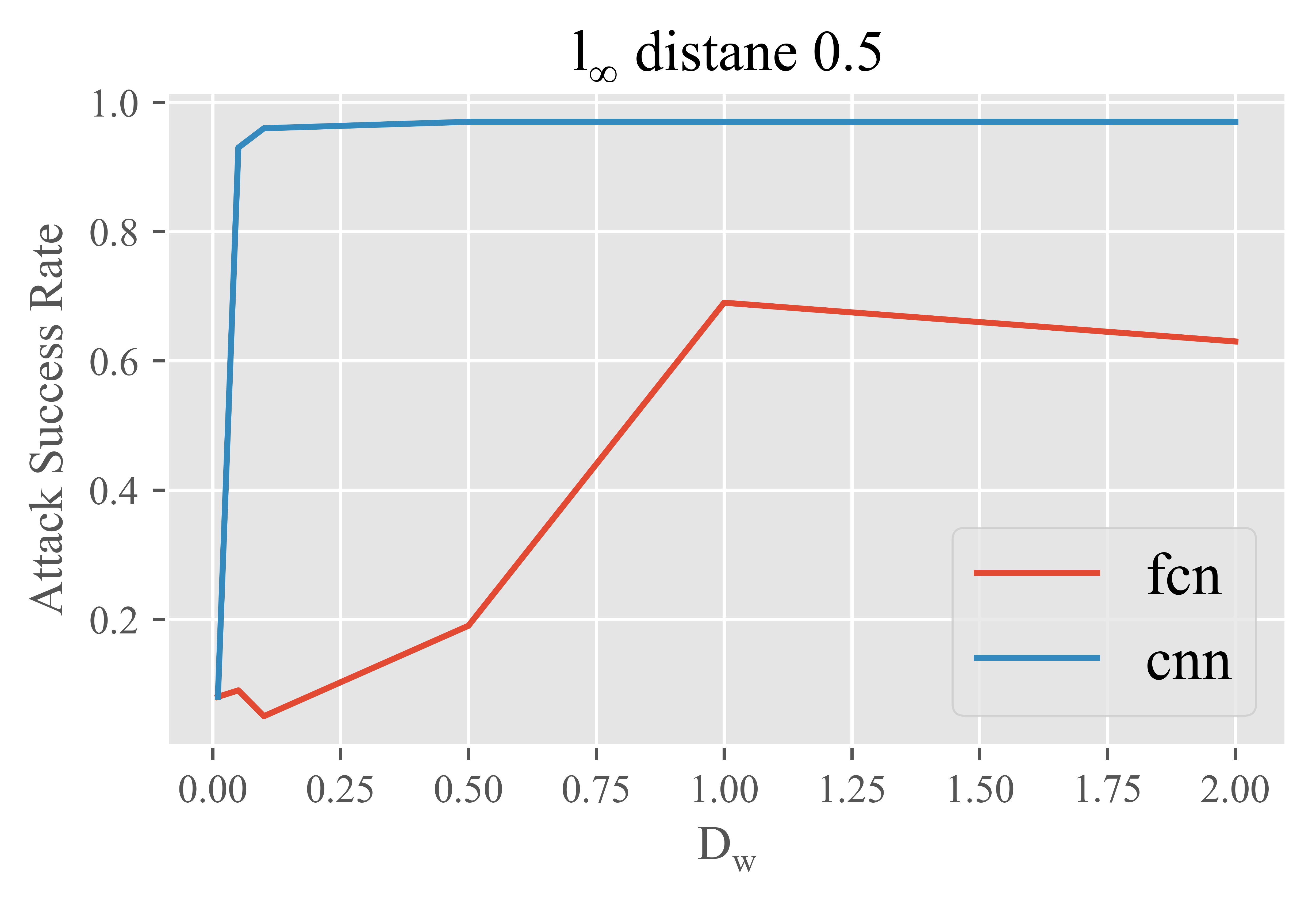
(a) ECG5000

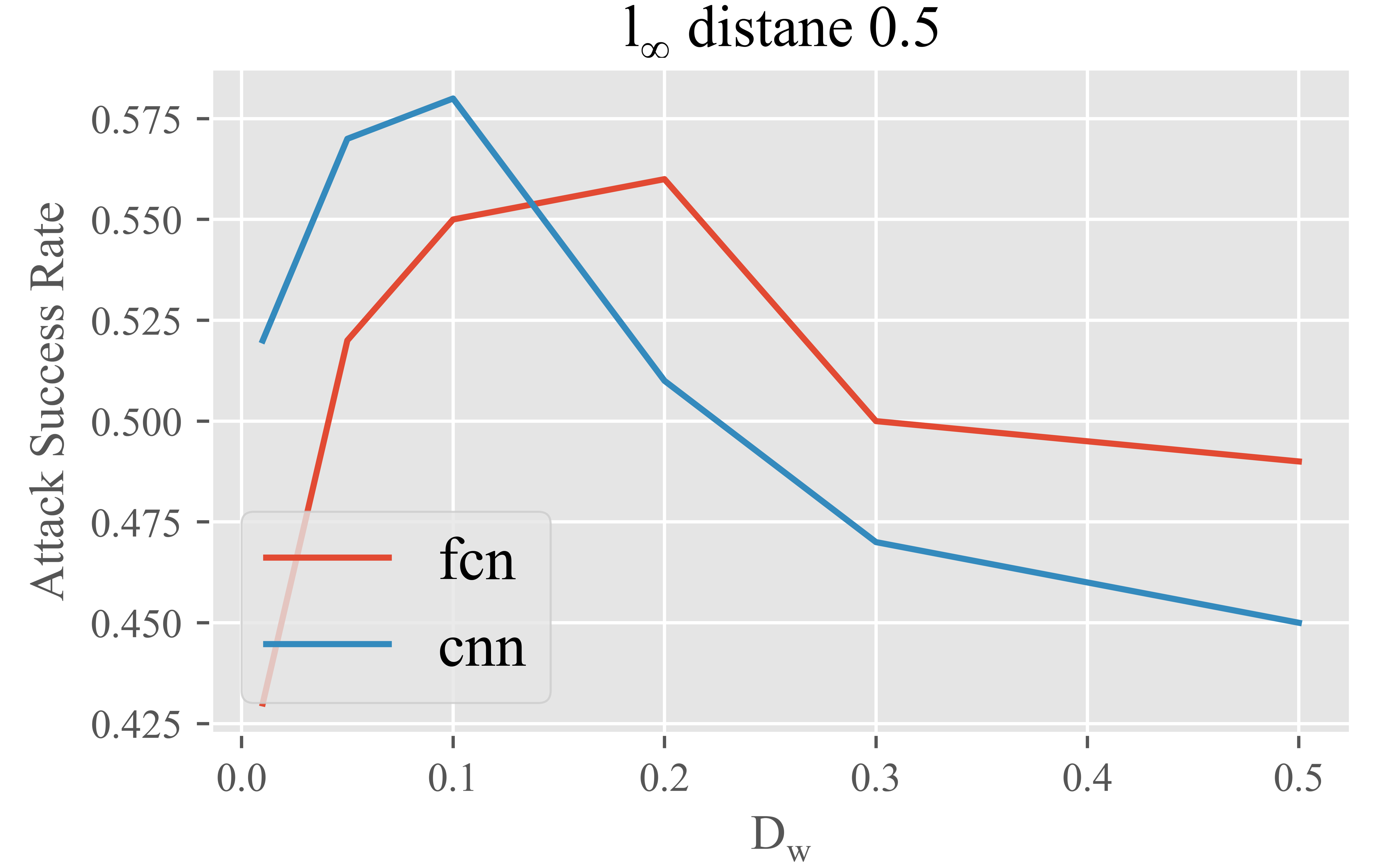
(b) ECG200

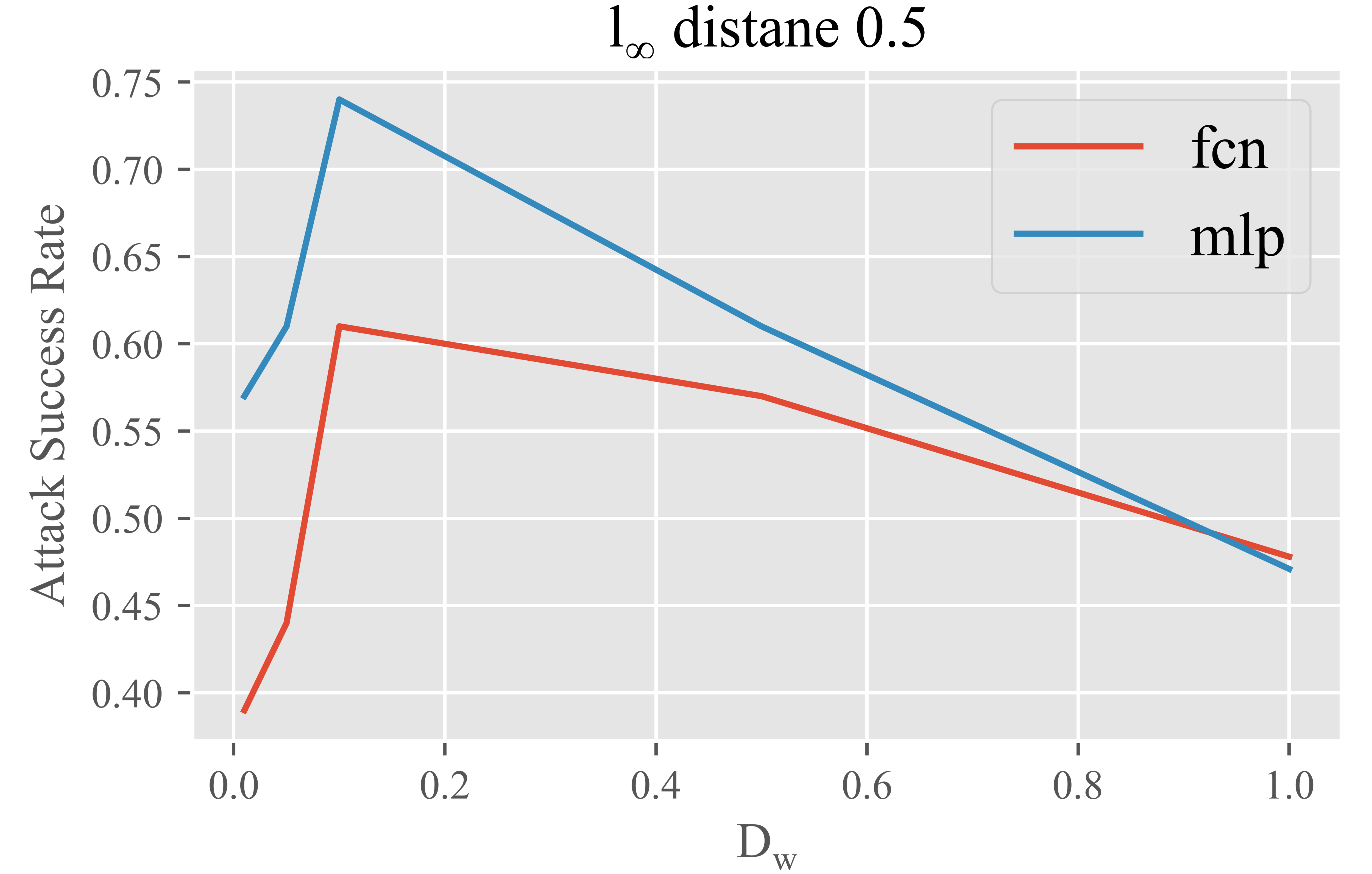
(c) ECGFiveDays

Figure 3. Attack Success Rate under different $\l_{\infty}$ and Wasserstein Bound: The columns represent the three dataset respectively.The first row illustrate under the same Wasserstein distance bound, how the attack success rate change with the increase of the $\l_{\infty}$ bound; The Second row illustrate under the same $\l_{\infty}$ bound, how the attack success rate change with the increase of the Wasserstein distance bound.

4.1. Experimental Setup

Our experiments are evaluated on Five benchmark time series classification datasets from the publicly available UCR archive (Chen et al., 2015). The datasets are selected under the “ECG” category for ECG based diagnosis tasks, where an adversarial attack is a potential security concern. In this section, we only show the results on three of the five ECG dataset, which are: 1) ECG200 which includes two classes (normal heartbeat and Myocardial Infarction), and contains 35 half-hour records sampled with the rate of 125 Hz. 2) ECG5000 which is the Beth Israel Deaconess Medical Center (BIDMC) congestive heart failure database, consisting of records of 15 subjects, with severe congestive heart failure. Five labels refes to different levels of heart failure. Records of each individual were recorded in 20 hours, containing two ECG signals, sampled with the rate of 250 Hz. 3) ECGFiveDays which is from a 67-year-old male, including two classes which are two ECG dates. We relegate the full version of the experiments of the other two datasets to the Appendix.

We adopt and evaluate the target deep learning models from (Ismail Fawaz et al., 2019c) including: Multi-Layer Perceptron (MLP) (Gardner and Dorling, 1998), Fully Connected Networks (FCN)(Long et al., 2015), Convolutional Neural Networks (CNN) (Krizhevsky et al., 2012) and Residual Networks (ResNet) (He et al., 2016). The detailed information of the ECG datasets and the performance of the target models on each dataset is listed in Table 1.

4.2. Attack Success Rate

Our proposed 2-step projection Wasserstein PGD involves a first projection to a $L_{\infty}$ norm-ball and a second projection to a Wasserstein ball. Figure 3 illustrates the impact of these two projections by comparing the ASR under different $L_{\infty}$ and Wasserstein bounds. The first row shows under the same Wasserstein distance bound, how the ASR changes with the increase of the $L_{\infty}$ bound, while the Second row shows under the same $\L_{\infty}$ bound, how the ASR changes with the increase of the Wasserstein distance bound. Each column represents the results of each dataset and each line in each figure corresponds to a target model. We show two models for each dataset and relegate the full version of the experiments to the Appendix.

Under the same radius of Wasserstein ball, the general trend is that ASR first increases with the increase of $L_{\infty}$ bound. This is intuitive as the search space for optimal adversarial examples that satisfy the Wasserstein distance constraint is increasing. It is easier to find an adversarial example that successfully attack the target model and meanwhile satisfy the Wasserstein constraint. However, as the $L_{\infty}$ bound keeps increasing, it does not help anymore and even hurts the performance because the search in the Wasserstein Space is not guided and constrained any more and can be too large for the projection to find a good solution. Therefore, the ASR stops increasing or starts to decrease. This decreasing trend is more noticeable in ECG200 and ECGFiveDays datasets, while for ECG5000, the ASR increases to and stays at 1 (for the CNN model). Note that our attack is untargeted attack that aims to flip the label to any class other than the original label rather than the targeted label. Therefore, multi-class classification task (ECG5000) is easier to attack than binary classification tasks (ECG200 and ECGFiveDays).

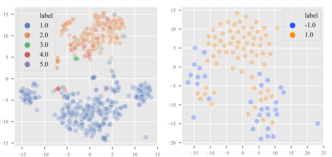
Figure 4. t-sne for ECG5000 (left) and ECG200 (right)

To further explain the difference between the datasets, we use t-distributed stochastic neighbor embedding (t-SNE), a nonlinear dimensionality reduction technique for high-dimensional visualization in a low-dimensional space (van der Maaten and Hinton, 2008), to visualize the datasets. Figure 4 shows the 2D t-sne for ECG200 and ECG5000 respectively. Each color represents a class label. We can note that data points of ECG200 is more separable and the class boundary is more clear, while the classes are overlapping for ECG5000 and the boundary is less clear, which makes it easier to attack. This explains why for ECG5000, the ASR increases to 1 and does not decrease.

On the other hand, under the same $L_{\infty}$ bound shown in the bottom row of Figure 3, larger Wasserstein bound also renders higher ASR at first due to larger search space. As it keeps increasing, the ASR decreases due to the search space being too large and the ineffectiveness of the search, especially when the radius of Wasserstein ball is greater than the Euclidean ball. Overall, the ASR of ECG5000, ECG200 and ECGFivedays can reach 100%, 62% and 74% respectively.

4.3. Effectiveness of 2-step Projection

From the perspective of ASR, we compare the 2-step projection with the direct 1-step Wasserstein projection shown as the dotted lines in the top row of Figure 3 under the same attack settings. We observe that 2-step projection can achieve a higher ASR in general and optimal attack success rate when choosing the proper $L_{\infty}$ bound for the first projection.

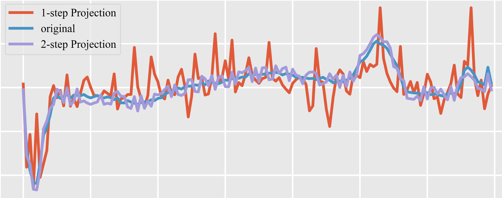
Figure 5. Comparison between direct Wasserstein projection (1-step projection) and 2-step projection.

From the perspective of human inspection, Figure 5 shows two successful adversarial examples generated by the 2-step projection (purple) and direct projection (red) respectively in comparison with the original example (blue). Although the Wasserstein perturbation distances of the two adversarial examples are both 0.99, the one that is first norm clipped is more imperceptible to human eyes, which has not only small Wasserstein distance but also bounded by $L_{\infty}$ distance.

4.4. Comparison with $L_{\infty}$ PGD

The intuition of developing the Wasserstein PGD attack is to search for more indistinguishable and natural adversarial examples in the Wasserstein space. Therefore, we compare the adversarial examples generated by Wasserstein PGD with those generated by original PGD in the Euclidean space ($L_{\infty}$ PGD). On one hand, We draw the utility comparison from two aspects: 1) Under the same attack success rate, Wasserstein PGD is more natural; and 2) Under the same perturbation scale, Wasserstein PGD has a higher attack success rate. On the other hand, as Wasserstein projection involves gradient descent which will add more time cost in generating adversarial examples, we also compare the average time cost of two attack methods.

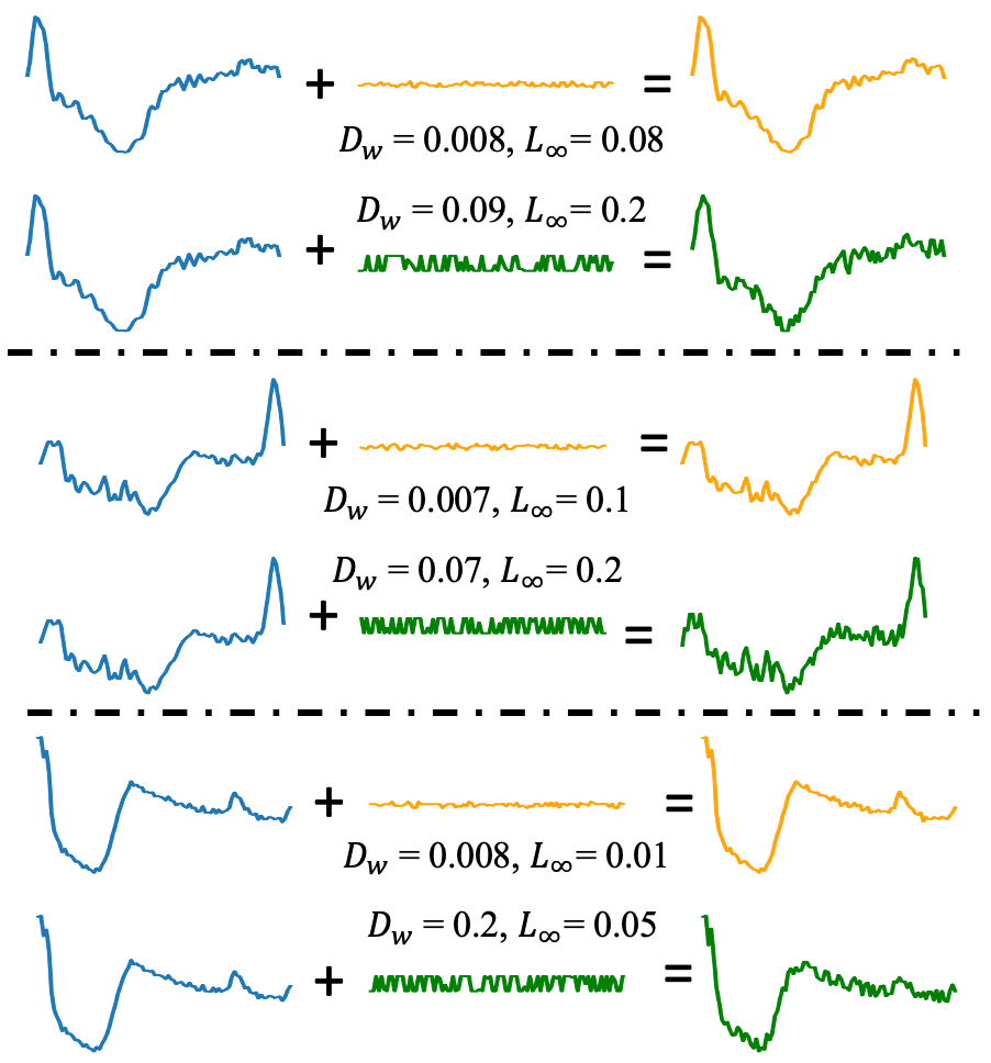
Figure 6. Comparison between Wasserstein PGD (yellow) and $L_{\infty}$ PGD (green) under the same attack success rate.

4.4.1. Under the same attack success rate, Wasserstein PGD is more natural

Figure 6 illustrates several comparisons between Wasserstein PGD and $L_{\infty}$ PGD under the same ASR. We selected three examples randomly. For each figure, the blue curve is the original input. The yellow curves represent the perturbation and adversarial example generated by Wasserstein PGD, while the green curves represent the $L_{\infty}$ PGD. Clearly, the perturbation generated from Wasserstein PGD is smaller and more indistinguishable than $L_{\infty}$ PGD.

4.4.2. Under the same perturbation scale, Wasserstein PGD has a higher attack success rate.

Another aspect to show the effectiveness of Wasserstein PGD is to compare the ASR with the original PGD under the same perturbation scale. However, the two attacks are conducted in different spaces. It is unfair to compare the ASR of adversarial examples generated from the Wasserstein ball and the $L_{\infty}$ ball with the same radius, as they represent completely different spaces. To overcome this challenge, we use the greatest $L_{\infty}$ norm of the Wasserstein examples as the radius of $L_{\infty}$ ball to generate $L_{\infty}$ PGD adversarial examples. For example, the maximum $L_{\infty}$ norm of the Wasserstein adversarial examples with 0.01 Wasserstein distance is 0.2. Then we will search for adversarial examples in the $L_{\infty}$ ball with the radius equal to 0.2. In this way, we have a fair comparison between the Wasserstein PGD and the original PGD attack.

Figure 7 shows the comparison of ASR in the way we introduced above. The x-axis refers to different attack settings corresponding to different Wasserstein and $L_{\infty}$ bounds (note that we have two steps of projections, first to an $L_{\infty}$ norm ball and second to a Wasserstein ball, while original PGD only uses $L_{\infty}$ projection). The purple and orange lines correspond to the Wasserstein PGD and original PGD respectively. We can note that in most cases, Wasserstein PGD has a higher attack success rate than the original attack.

From these two aspects, we can conclude that for univariant time series data, Wasserstein PGD not only can generate more natural adversarial examples but also can achieve a higher ASR under the same attack scale.

Figure 7. Comparison between Wasserstein PGD and $l_{\infty}$ PGD under the same attack scale.

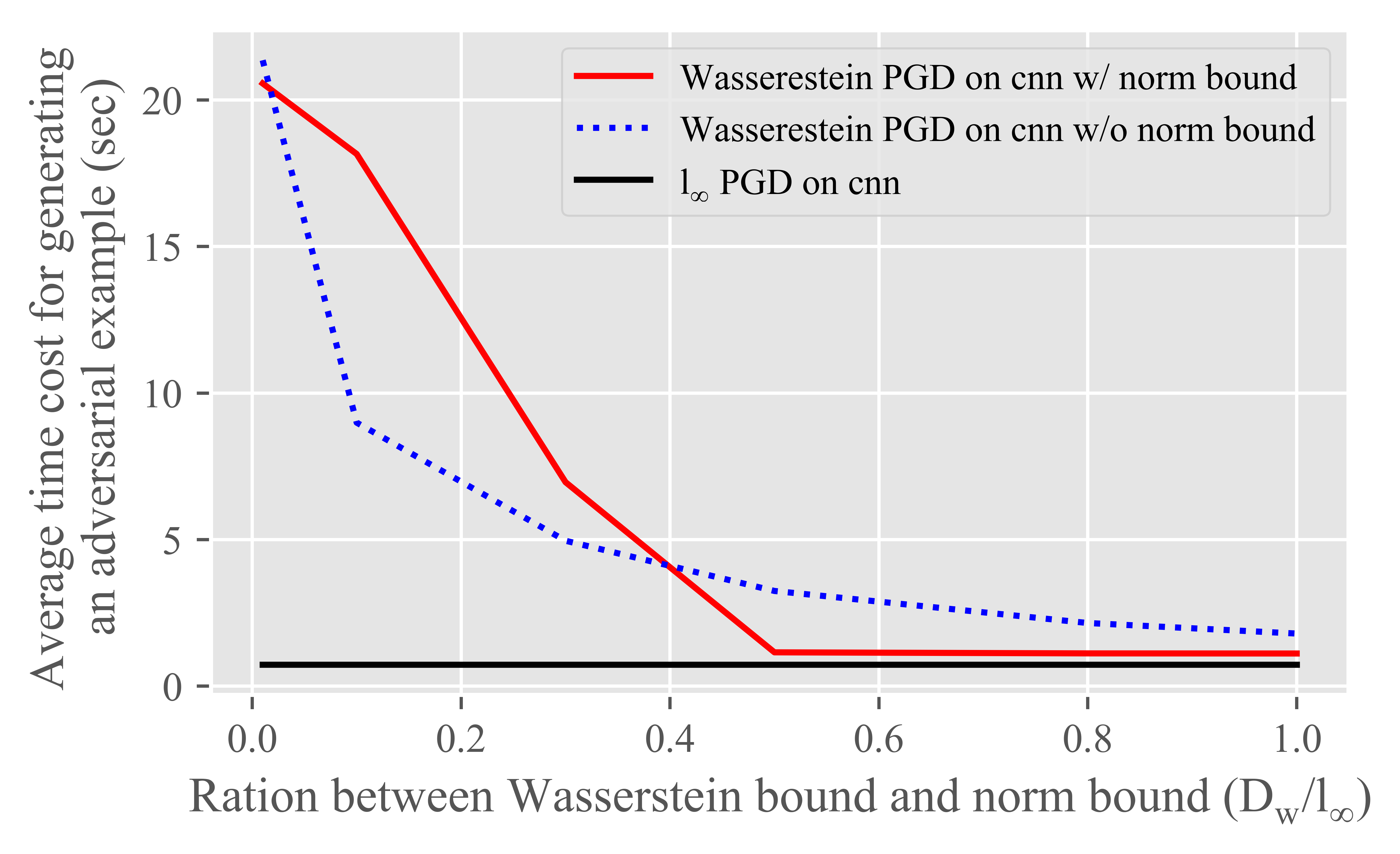
(a) ECG200 CNN

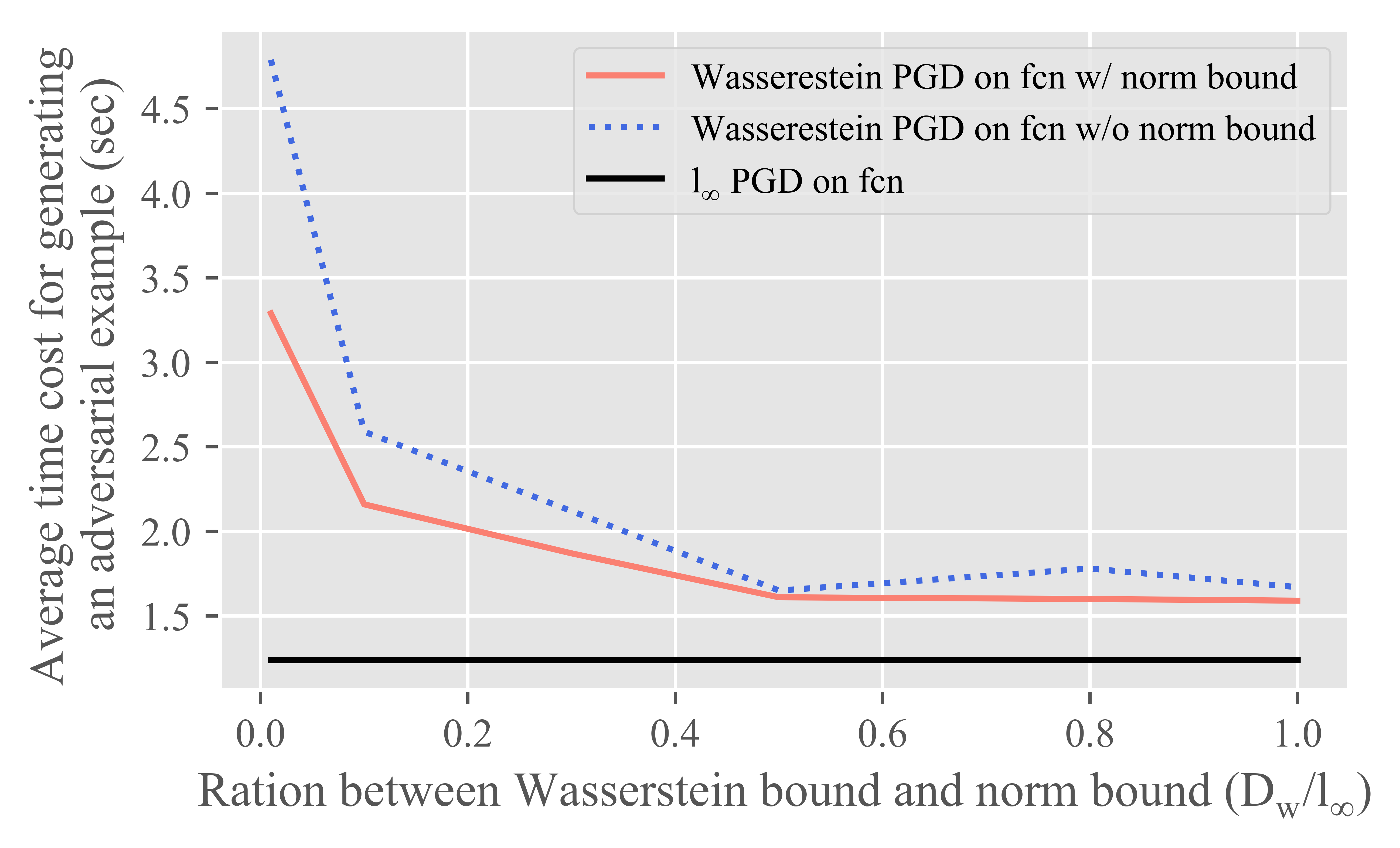
(b) ECG200 FCN

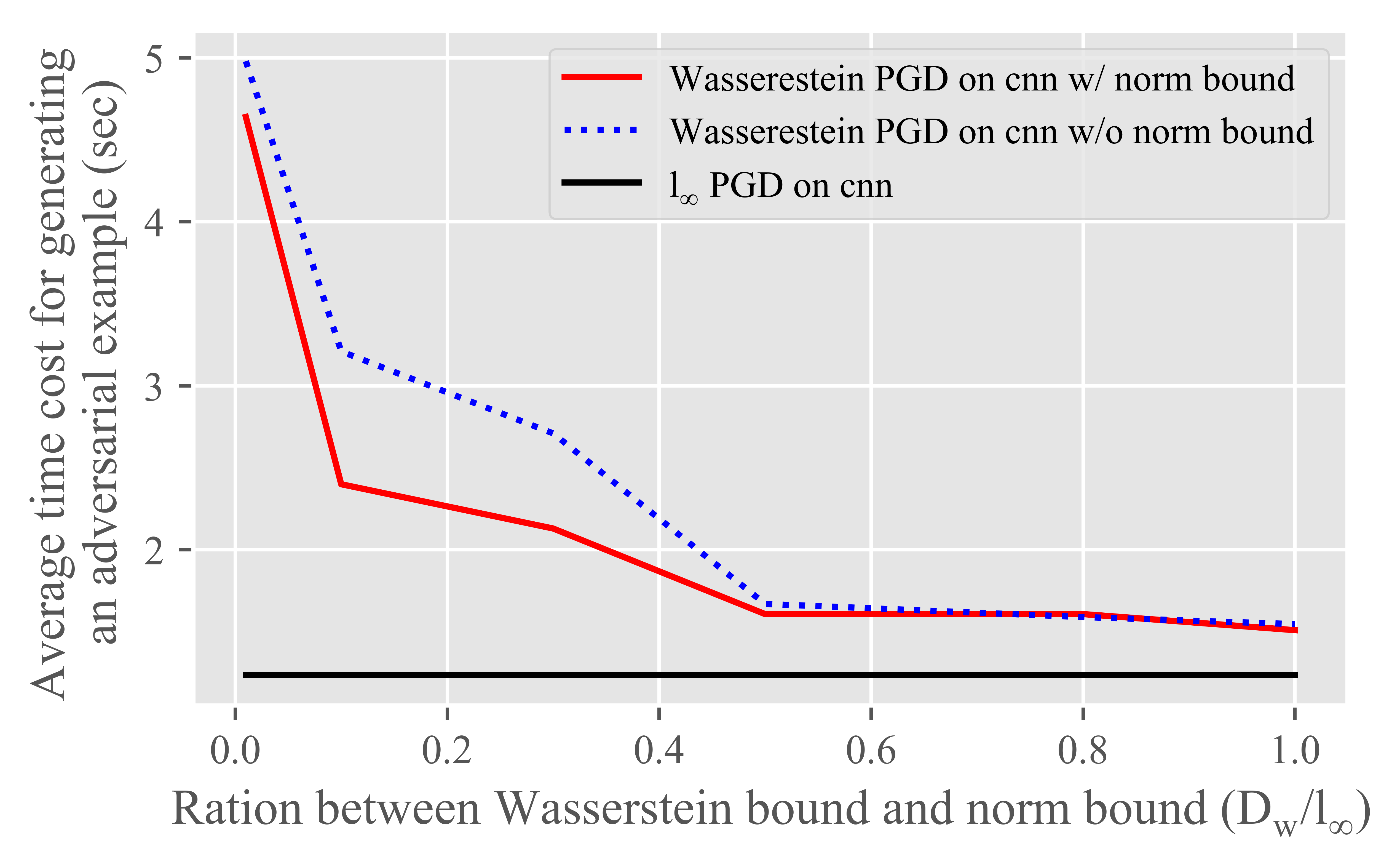
(c) ECG5000 CNN

(d) ECG5000 FCN

Figure 8. The average time cost of generating an adversarial example with Wasserstien PGD (with and without norm bound clipping) and $L_{\infty}$ PGD attack.

4.4.3. Compare the time cost between Wasserstein PGD and $L_{\infty}$ PGD

Besides comparing the utility of Wasserstein PGD with $L_{\infty}$ PGD, we also evaluate how Wasserstein PGD increases the time cost by comparing the average time cost of generating an adversarial example with $L_{\infty}$ PGD attack, as Wasserstein PGD involves projection into the Wasserstein ball via gradient which will result in more time cost. As the time cost of the Wasserstein projection is largely relative to the size of $L_{\infty}$ ball (the start point of gradient descent) and the size of the Wasserstein ball (the destination), we compare the average time cost according to the ratio between Wasserstein bound and $L_{\infty}$ bound.

As shown in Figure 8, the red and blue curves are the Wasserstein PGD with and without the first stage of norm clipping, while the black line represents the baseline $L_{\infty}$ PGD attack, whose value is irrelevant to the ratio between Wasserstein and $L_{\infty}$ bound. We show the result on two datasets and two models: ECG200 and ECG5000, with CNN and FCN models. We can note that Wasserstein PGD will result in more time cost than $L_{\infty}$ PGD, especially when the ratio between Wasserstein bound and $L_{\infty}$ bound is large. However, when the ratio approaches 1, this increase in time cost is neglectable. By comparing the red and blue curves we can conclude that when the ratio between the Wasserstein bound and $L_{\infty}$ bound approaches 1, the first stage of norm clipping can effectively guide the search for Wasserstein adversarial examples. However, when the ratio increases( approaches 0), even with the bound of norm clipping, the search also tends to be a random search.

4.5. Countermeasure against Wasserstein PGD

To better study the nature of Wasserstein adversarial examples, we also explored certified robustness approach as a potential defense mechanism for Wasserstein PGD. We consider certified robustness in contrast to other empirical defense methods as it is the most powerful and principled defense method to date.

We adopt Wasserstein smoothing (Levine and Feizi, 2020) which is originally designed for image data not the univariant time series data. The basic idea of Wasserstein smoothing is to define a reduced transport plan and map the Wasserstein distance on the input space to the $L_{1}$ norm on the transport plan. The base classifier is transformed into a smoothed classifier by adding Laplacian noise $Laplace(0,\sigma)^{r}$ to the reduced transport plan, where $r$ is corresponding to the input dimension. Because of the mapping, smoothing in the transport domain can be performed using existing $L_{1}$ robustness certification provided by (Lecuyer et al., 2019) and mapped back to the Wasserstein Space. The strict form of the certified condition can be stated as:

Theorem 1.

For any normalized probability distribution input $x\in\mathbb{R}^{n*m}$ with correct class $c$, if:

(8) $$\bar{f_{c}}(x)\geq e^{2\sqrt{2}\zeta/\sigma}(1-\bar{f_{c}}(x))$$

then for any perturbed $\tilde{x}$ that $d_{W}(x,\tilde{x})\leq\zeta$, we have

(9) $$\bar{f_{c}}(\tilde{x})\geq\underset{i\neq c}{max}\bar{{f_{i}}}(\tilde{x})$$

The detailed proof and the design of the reduced transport plan can be referred to (Levine and Feizi, 2020)

We evaluate how Wasserstein Smoothing empirically works on the proposed Wasserstein PGD attack with two evaluation metrics (Wang et al., 2021): Certified accuracy (CertAcc) which denotes the fraction of the clean testing set on which the predictions are correct and also satisfy the certification criteria. Formally, it is defined as: $\frac{\sum_{t=1}^{T}certifiedCheck(X_{t},L,\epsilon)\&corrClass(X_{t},L,\epsilon)}{T},$ where $certifiedCheck$ returns 1 if Theorem 1 is satisfied and $corrClass$ returns 1 if the classification output is correct. $T$ is the size of the test dataset. Conventional accuracy (ConvAcc) is defined as the fraction of testing set that is correctly classified, $\frac{\sum_{t=1}^{T}corrClass(X_{t},L,\epsilon)}{T}$, which is a standard metric to evaluate any deep learning systems.

Figure 9 illustrates how the certified accuracy changes under different Wasserstein certified radius $\zeta$ in Equation 8. During the experiments, the Laplace parameter $\sigma$ which controls the noise to the transport plan is set to 0.01 and the soft prediction result is averaged over 100 times of sampling. As Wasserstein radius increases, the certified accuracy decreases, which means less fraction of examples can satisfy the certification condition in Equation 8. When Wasserstein radius $\zeta$ is set over 0.1, the certified accuracy stops decreasing. We can note from this result that: first, under a certain Laplacian distribution, the certified radius is limited. Second, to a very small certified radius, for examples less than 0.01, the certified accuracy can achieve 100%.

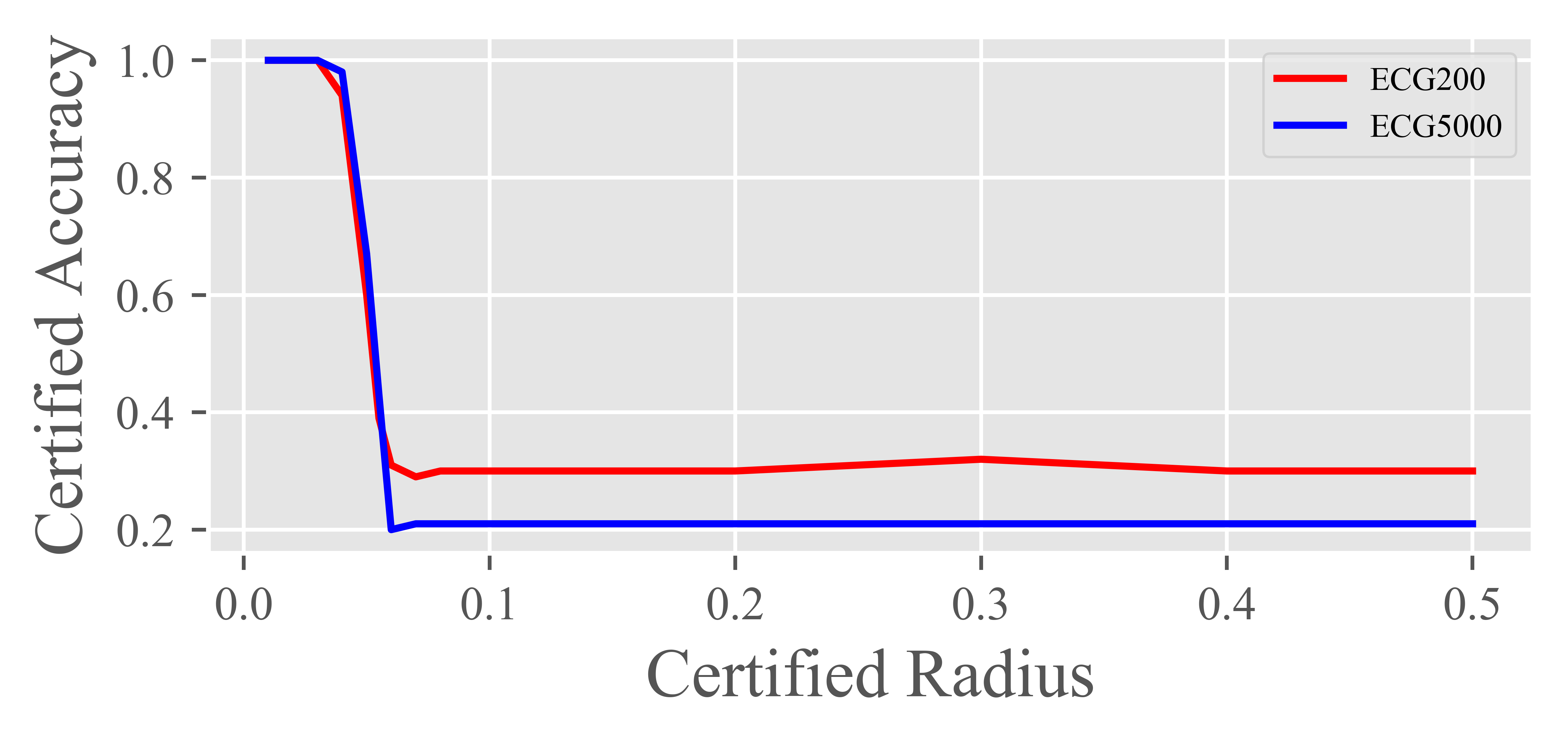
Figure 9. Comparison of Certified Accuracy under different Wasserstein radius with $\sigma=0.01$

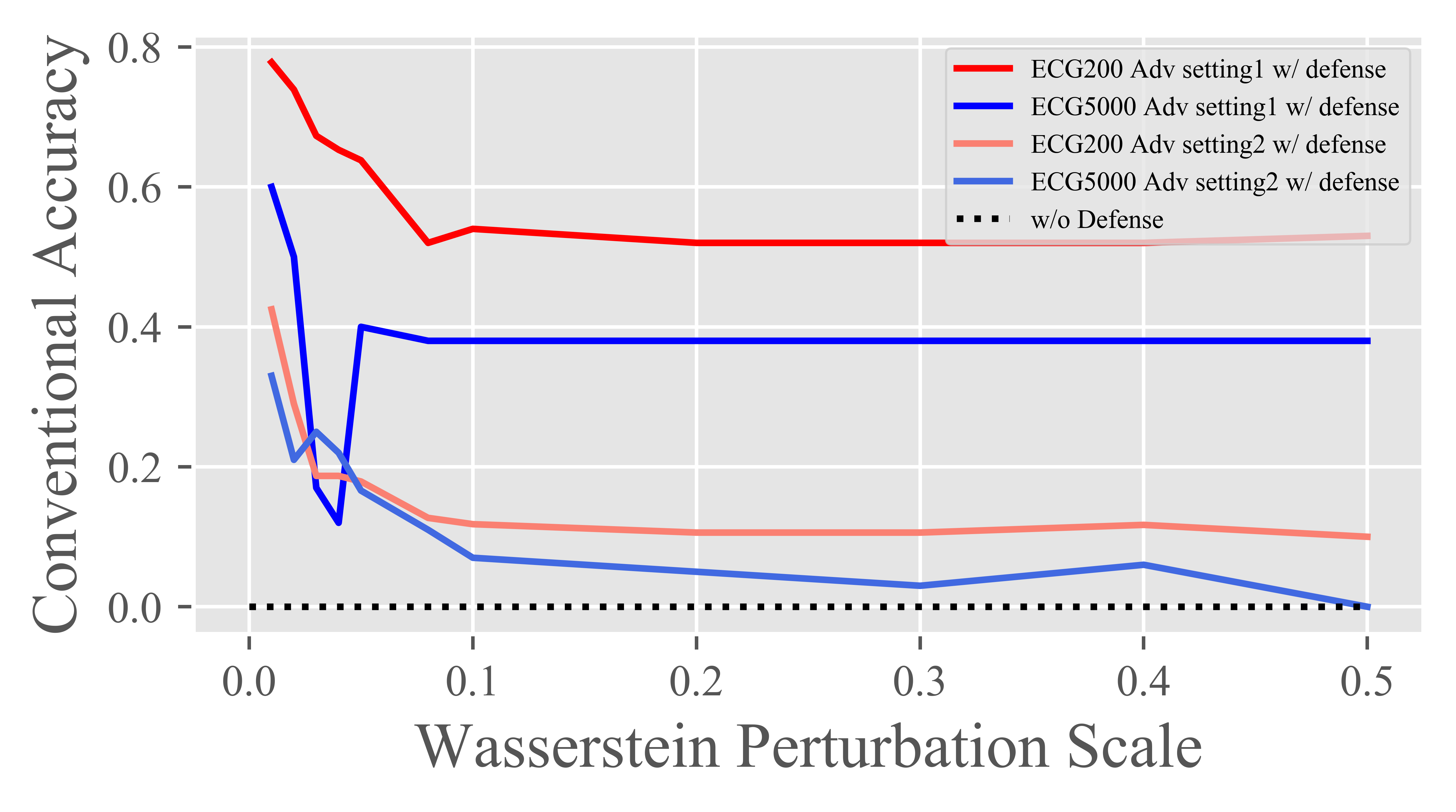
Figure 10. Comparison of Conventional Accuracy of successfully attacked adversarial examples.

Figure 10 demonstrates whether Wasserstein smoothing can empirically increase the conventional accuracy of adversarial examples generated by Wasserstein PGD. In the experiments, we test on successfully generated adversarial examples, so the baseline accuracy of the dataset is 0. Laplace parameter $\sigma$ is set to 0.1 and the soft prediction result is averaged over 100 times of sampling. The x-axis refers to the Wasserstein attack scales. The two red lines represent the adversarial examples generated from ECG200 under two different settings, $L_{\infty}$ norm set to 0.1 and 0.2, and the two blue lines represent the adversarial examples generated from ECG5000 where $L_{\infty}$ norm set to 0.1 and 0.2. We can note from the figures the following. First, when the Wasserstein attack scales are small, Wasserstein smoothing can render some accuracy gain. The accuracy decreases with the increase of Wasserstein perturbation scales as expected. When the Wasserstein distance increase over 0.06, which is also the greatest certified radius, the accuracy gain is limited and does not change anymore. We also randomly select two adversarial examples with Wasserstein perturbations around 0.06. As shown in Figure 11, the adversarial ECG is fairly indistinguishable to human eyes. Yet Wasserstein Smoothing can not provide reasonable defense at this level. Second, with ECG200 and ECG5000 under setting2 ( $L_{\infty}$ norm set to 0.2), the overall accuracy gain is very small for all perturbation scales.

We can conclude from the results that the existing Wasserstein smoothing has limited success in both certified ratio and conventional accuracy gain. This suggests that there is still space for developing stronger certified robustness method to Wasserstein PGD tailored to time series data instead of using the general transport plan based smoothing designed for image data.

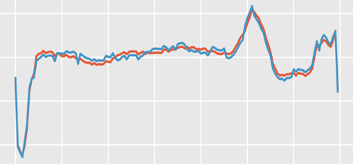
Figure 11. The comparison between adversarial examples and clean examples at $d_{\mathcal{W}}$ scale around 0.06.

5. Conclusion

We proposed the Wasserstein PGD attack for univariant time series data, which is the first effort to study adversarial example attacks on time series in the Wasserstein space. Compared with the original PGD attack in the Euclidean space, Wasserstein PGD can generate more imperceptible and natural adversarial examples. Extensive results showed that Wasserstein PGD can achieve higher ASR with smaller perturbations. We also explored certified robustness via Wasserstein smoothing as a potential defense method. The results showed that Wasserstein smoothing has limited certified range and accuracy gain. In the future, it would be interesting to study Wasserstein adversarial examples on multivariant time series under Gaussian distributions. Stronger certified robustness methods can also be developed by designing reduced transport plan that is more suitable for time series data.

References

- (1)
- Alt and Godau (1995) Helmut Alt and Michael Godau. 1995. Computing the Fréchet distance between two polygonal curves. International Journal of Computational Geometry & Applications 5, 01n02 (1995), 75–91.
- Baluja and Fischer (2017) Shumeet Baluja and Ian Fischer. 2017. Adversarial Transformation Networks: Learning to Generate Adversarial Examples. arXiv:1703.09387 [cs.NE]
- Berndt and Clifford (1994) Donald J Berndt and James Clifford. 1994. Using dynamic time warping to find patterns in time series.. In KDD workshop, Vol. 10. Seattle, WA, USA:, 359–370.
- Carlini and Wagner (2017) Nicholas Carlini and David Wagner. 2017. Towards evaluating the robustness of neural networks. In 2017 ieee symposium on security and privacy (sp). Ieee, 39–57.
- Castells et al. (2007) Francisco Castells, Pablo Laguna, Leif Sörnmo, Andreas Bollmann, and José Millet Roig. 2007. Principal component analysis in ECG signal processing. EURASIP Journal on Advances in Signal Processing 2007 (2007), 1–21.
- Chen et al. (2015) Yanping Chen, Eamonn Keogh, Bing Hu, Nurjahan Begum, Anthony Bagnall, Abdullah Mueen, and Gustavo Batista. 2015. The UCR Time Series Classification Archive. www.cs.ucr.edu/~eamonn/time_series_data/.
- Cohen et al. (2019) Jeremy Cohen, Elan Rosenfeld, and Zico Kolter. 2019. Certified adversarial robustness via randomized smoothing. In International Conference on Machine Learning. PMLR, 1310–1320.
- Gardner and Dorling (1998) Matt W Gardner and SR Dorling. 1998. Artificial neural networks (the multilayer perceptron)—a review of applications in the atmospheric sciences. Atmospheric environment 32, 14-15 (1998), 2627–2636.
- Goodfellow et al. (2014) Ian J Goodfellow, Jonathon Shlens, and Christian Szegedy. 2014. Explaining and harnessing adversarial examples. arXiv preprint arXiv:1412.6572 (2014).
- He et al. (2016) Kaiming He, Xiangyu Zhang, Shaoqing Ren, and Jian Sun. 2016. Deep residual learning for image recognition. In Proceedings of the IEEE conference on computer vision and pattern recognition. 770–778.
- Ismail Fawaz et al. (2019a) Hassan Ismail Fawaz, Germain Forestier, Jonathan Weber, Lhassane Idoumghar, and Pierre-Alain Muller. 2019a. Adversarial Attacks on Deep Neural Networks for Time Series Classification. 2019 International Joint Conference on Neural Networks (IJCNN) (Jul 2019). https://doi.org/10.1109/ijcnn.2019.8851936
- Ismail Fawaz et al. (2019b) Hassan Ismail Fawaz, Germain Forestier, Jonathan Weber, Lhassane Idoumghar, and Pierre-Alain Muller. 2019b. Deep learning for time series classification: a review. Data Mining and Knowledge Discovery 33, 4 (Mar 2019), 917–963. https://doi.org/10.1007/s10618-019-00619-1
- Ismail Fawaz et al. (2019c) Hassan Ismail Fawaz, Germain Forestier, Jonathan Weber, Lhassane Idoumghar, and Pierre-Alain Muller. 2019c. Deep learning for time series classification: a review. Data mining and knowledge discovery 33, 4 (2019), 917–963.
- Karim et al. (2021) Fazle Karim, Somshubra Majumdar, and Houshang Darabi. 2021. Adversarial Attacks on Time Series. IEEE Transactions on Pattern Analysis and Machine Intelligence 43, 10 (Oct 2021), 3309–3320. https://doi.org/10.1109/tpami.2020.2986319
- Karim et al. (2019) Fazle Karim, Somshubra Majumdar, Houshang Darabi, and Samuel Harford. 2019. Multivariate LSTM-FCNs for time series classification. Neural Networks 116 (2019), 237–245.
- Krizhevsky et al. (2012) Alex Krizhevsky, Ilya Sutskever, and Geoffrey E Hinton. 2012. Imagenet classification with deep convolutional neural networks. Advances in neural information processing systems 25 (2012).
- Kurakin et al. (2016) Alexey Kurakin, Ian Goodfellow, and Samy Bengio. 2016. Adversarial examples in the physical world. arXiv preprint arXiv:1607.02533 (2016).
- Kurakin et al. (2018) Alexey Kurakin, Ian J Goodfellow, and Samy Bengio. 2018. Adversarial examples in the physical world. In Artificial intelligence safety and security. Chapman and Hall/CRC, 99–112.
- Lecuyer et al. (2019) Mathias Lecuyer, Vaggelis Atlidakis, Roxana Geambasu, Daniel Hsu, and Suman Jana. 2019. Certified Robustness to Adversarial Examples with Differential Privacy. 2019 IEEE Symposium on Security and Privacy (SP) (May 2019). https://doi.org/10.1109/sp.2019.00044
- Levine and Feizi (2020) Alexander Levine and Soheil Feizi. 2020. Wasserstein smoothing: Certified robustness against wasserstein adversarial attacks. In International Conference on Artificial Intelligence and Statistics. PMLR, 3938–3947.
- Long et al. (2015) Jonathan Long, Evan Shelhamer, and Trevor Darrell. 2015. Fully convolutional networks for semantic segmentation. In Proceedings of the IEEE conference on computer vision and pattern recognition. 3431–3440.
- Ma et al. (2018) Tengfei Ma, Cao Xiao, and Fei Wang. 2018. Health-ATM: A Deep Architecture for Multifaceted Patient Health Record Representation and Risk Prediction. In SDM.
- Madry et al. (2017) Aleksander Madry, Aleksandar Makelov, Ludwig Schmidt, Dimitris Tsipras, and Adrian Vladu. 2017. Towards deep learning models resistant to adversarial attacks. arXiv preprint arXiv:1706.06083 (2017).
- McSherry and Talwar (2007) Frank McSherry and Kunal Talwar. 2007. Mechanism design via differential privacy. In 48th Annual IEEE Symposium on Foundations of Computer Science (FOCS’07). IEEE, 94–103.
- Mode and Hoque (2020) Gautam Raj Mode and Khaza Anuarul Hoque. 2020. Adversarial Examples in Deep Learning for Multivariate Time Series Regression. 2020 IEEE Applied Imagery Pattern Recognition Workshop (AIPR) (Oct 2020). https://doi.org/10.1109/aipr50011.2020.9425190
- Neyman and Pearson (1992) J. Neyman and E. S. Pearson. 1992. On the Problem of the Most Efficient Tests of Statistical Hypotheses. Springer New York, New York, NY, 73–108. https://doi.org/10.1007/978-1-4612-0919-5_6
- Szegedy et al. (2013) Christian Szegedy, Wojciech Zaremba, Ilya Sutskever, Joan Bruna, Dumitru Erhan, Ian Goodfellow, and Rob Fergus. 2013. Intriguing properties of neural networks. arXiv preprint arXiv:1312.6199 (2013).
- Tobiyama et al. (2016) Shun Tobiyama, Yukiko Yamaguchi, Hajime Shimada, Tomonori Ikuse, and Takeshi Yagi. 2016. Malware Detection with Deep Neural Network Using Process Behavior. In 2016 IEEE 40th Annual Computer Software and Applications Conference (COMPSAC), Vol. 2. 577–582. https://doi.org/10.1109/COMPSAC.2016.151
- Vallender (1974) SS Vallender. 1974. Calculation of the Wasserstein distance between probability distributions on the line. Theory of Probability & Its Applications 18, 4 (1974), 784–786.
- van der Maaten and Hinton (2008) Laurens van der Maaten and Geoffrey Hinton. 2008. Visualizing Data using t-SNE. Journal of Machine Learning Research 9, 86 (2008), 2579–2605. http://jmlr.org/papers/v9/vandermaaten08a.html
- Wang et al. (2021) Wenjie Wang, Pengfei Tang, Jian Lou, and Li Xiong. 2021. Certified robustness to word substitution attack with differential privacy. In Proceedings of the 2021 Conference of the North American Chapter of the Association for Computational Linguistics: Human Language Technologies. 1102–1112.
- Wong et al. (2019) Eric Wong, Frank R. Schmidt, and J. Zico Kolter. 2019. Wasserstein Adversarial Examples via Projected Sinkhorn Iterations. arXiv:1902.07906 [cs.LG]