Plasma kinetics: Discrete Boltzmann modeling and Richtmyer-Meshkov instability

Abstract

A discrete Boltzmann model (DBM) for plasma kinetics is proposed. The constructing of DBM mainly considers two aspects. The first is to build a physical model with sufficient physical functions before simulation. The second is to present schemes for extracting more valuable information from massive data after simulation. For the first aspect, the model is equivalent to a magnetohydrodynamic model plus a coarse-grained model for the most relevant TNE behaviors including the entropy production rate. A number of typical benchmark problems including Orszag-Tang (OT) vortex problem are used to verify the physical functions of DBM. For the second aspect, the DBM use non-conserved kinetic moments of ($f-f^{eq}$) to describe non-equilibrium state and behaviours of complex system. The OT vortex problem and the Richtmyer-Meshkov instability (RMI) are practical applications of the second aspect. For RMI with interface inverse and re-shock process, it is found that, in the case without magnetic field, the non-organized momentum flux shows the most pronounced effects near shock front, while the non-organized energy flux shows the most pronounced behaviors near perturbed interface. The influence of magnetic field on TNE effects shows stages: before the interface inverse, the TNE strength is enhanced by reducing the interface inverse speed; while after the interface inverse, the TNE strength is significantly reduced. Both the global average TNE strength and entropy production rate contributed by non-organized energy flux can be used as physical criteria to identify whether or not the magnetic field is sufficient to prevent the interface inverse.

I Introduction

As the fourth state of matter, plasma exists extensively in natural and various industrial fields such as initial confinement fusion (ICF). Betti and Hurricane (2016); Abu-Shawareb et al. (2022) In ICF, the target pellet is driven by strong laser or x ray, which ionizes the shell ablator material and forms strong shock waves to compress the fuel centrally to a high temperature and density of the ignition state. When the imposing shock wave passes through a perturbed interface, the perturbation amplitude increases with time, resulting in the mix of ablator material into the fuel plasmas and even causing ignition failure. Brouillette (2002) This phenomenon was first investigated theoretically by RichtmyerRichtmyer; (1960) through linear stability analysis, then qualitatively verified by Meshkov Meshkov (1969) through shock tube experiments. Now, it is generally referred to as the Richtmyer-Meshkov instability (RMI). As a physical phenomenon that is bound to occur when certain conditions are met, the RMI also plays important roles in astrophysics Arnett (2000); Sano et al. (2021), shock wave physics, combustion Khokhlov, Oran, and Thomas (1999) and other kinds of systems Zhou (2017a, b); Zhou et al. (2021).

Due to the importance and complexity of RMI, extensive theoretical, experimental and numerical studies have been carried out. Zhai et al. (2011); Xu et al. (2016); Lei et al. (2017); Zhou (2017a, b); Wang et al. (2017); Zhai et al. (2018) Among them, plasma RMI is one of the important research areas. Previous theoretical and numerical studies for plasma RMI are mainly based on two kinds of models. The first kinds are various magnetohydrodynamics (MHD) models which simultaneously couple Euler/Navier-Stokes (NS) equations with Maxwell equations. Based on MHD models, the effects of applied magnetic fields and self-generated electromagnetic fields on the development of plasma RMI have been extensively studied. Samtaney (2003); Wheatley, Pullin, and Samtaney (2005a, b); Wheatley, Samtaney, and Pullin (2009); Sano, Inoue, and Nishihara (2013); Wheatley et al. (2014); Mostert et al. (2015); Bond et al. (2017); Zhang et al. (2020); Qin and Dong (2021); Li, Bakhsh, and Samtaney (2022); Bakhsh (2022); Zhang et al. (2023) It should be noted that, the MHD model of NS level is based on quasi-continuum assumption, and consequently it is only valid when Knudsen number $Kn$ (defined as the ratio of molecular mean free path $l$ to a characteristic length scale $L$) is sufficient small. However, the local $Kn$ near the imposing plasma shock Vidal et al. (1993); Liu et al. (2023); Bond et al. (2017) or near the perturbed interface is generally so large that it challenges the validity of the continuum assumption,McMullen et al. (2022) resulting in inaccurate predictions of physical quantities. Zhang et al. (2019a, b); Qiu et al. (2021); Gan et al. (2022) Secondly, the MHD model is based on the near equilibrium assumption where only the first order Knudsen number effects are taken into account. From this perspective, the Knudsen number $Kn$ is regarded as the ratio of relaxation time $\tau$ to the time scale $T^{Rep}$ of a characteristic flow behavior. However, the local $Kn$ near the imposing plasma shock or near the perturbed interface is generally so large that higher order Knudsen number effects should be taken into account, and consequently challenges the validity of the near-equilibrium assumption, McMullen et al. (2022) resulting in rich and complex non-equilibrium behaviors.Xu and Zhang (2022) Generally, there exist two kinds of non-equilibrium behaviors. The first is hydrodynamic non-equilibrium (HNE), which refers to the non-equilibrium that could be described by hydrodynamic theory. The second is thermodynamic non-equilibrium (TNE), which refers to the non-equilibrium described by kinetic theory and due to that the distribution function $f$ deviates from its corresponding equilibrium distribution function $f^{eq}$. It is clear that the HNE is only a small portion of the TNE.Xu and Zhang (2022) It is meaningful to mention that, even for the case where the $Kn$ is small enough and consequently the NS description is reasonable, the NS shows deficiency or inconvenience for investigating some TNE behaviors, such as how the various TNE mechanisms influence the entropy production rates. Nowadays, TNE is attracting more attention with time, Chen and Zhao (2017); Qiu et al. (2020, 2021); Bao et al. (2022) but is still far from being fully understood. More seriously, the MHD model of Euler equation level corresponds to the case where the local Knudsen number is zero. It completely neglects the viscous and heat conductive effects.

The second kinds are some kinetic models based on the non-equilibrium statistical physics, mainly based on the Boltzmann equation. Those kinetic models can be classified into two types. The first type consider the particle collision, and the second type neglect the particle collision. Examples of the first type are as follows: Direct simulation Monte Carlo (DSMC) Bird (1998), particle-in-cell (PIC) Asahina et al. (2017), hybrid fluid-PIC (Cai et al., 2021) and Vlasov-Fokker-Planck (VFP) method Keenan et al. (2017); Larroche et al. (2016), etc. Some of these methods have provided a promising solution for studying the RMI. Meng et al. (2019); Kumar and Maheshwari (2020); Liu et al. (2020); Yan et al. (2021) The second type which neglects the particle collision and is based on the Vlasov equation. It is worth noting that a considerable part of the currently adopted kinetic models ignore collisions, while researchers point out that the kinetic effects caused by particle collisions have the potential to impact the ICF.Robey (2004); Rinderknecht et al. (2018); Cai et al. (2020); Yao et al. (2020); Cai et al. (2021); Lianqiang et al. (2020)

What the content above discuss are mainly for how to model the physical behavior aiming to study, which prepares the evolution equation combined with necessary physical constraints for theoretical and numerical investigation. It is well-known that, numerical experiment study includes mainly three steps: (i) physical modeling, (ii) discrete format design/selection, (iii) numerical experiment and complex physical field analysis, as shown in Fig. 1(a).

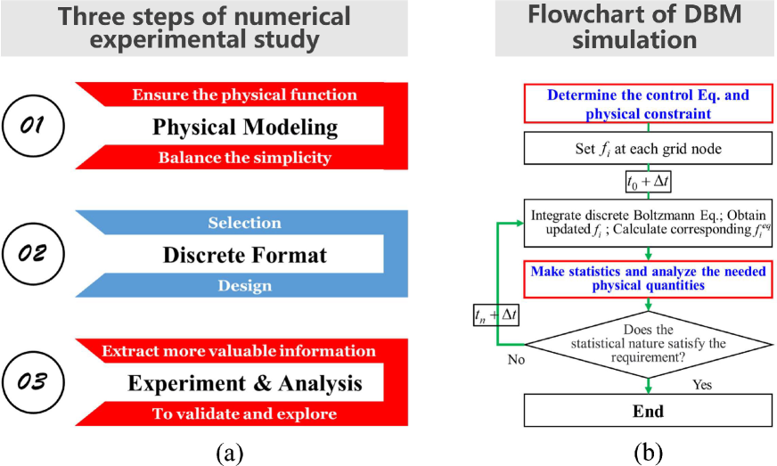
Figure 1: Flowcharts for numerical experimental study (a) and DBM simulation study (b).

Physics group generally focus mainly on steps (i) and (iii), while computational mathematics group generally focus on step (ii). After the numerical experiments, what we face are huge amount of data. All the models and methods mentioned above are for pre-simulation services, and are not responsible for post-simulation data analysis. Although we have made great progress in the analysis of complex physical fields, how much information do we extract from these huge amounts of data compared to the information contained in the data? Actually not optimistic. It can be said that most information is in a state of sleep. How to extract more reliable and valuable information from these data is the key to the further development of the research. For example, what kind of physical quantities are needed to identify and detect the discrete effects and non-equilibrium effects we mentioned above?

In order to solve the above problems, we can resort to the recent proposed discrete Boltzmann method (DBM).Xu and Zhang (2022); Xu et al. (2021a, b, c); Gan et al. (2022); Xu (2023) The DBM is developed from the physical modeling branch of LBM, Succi (2001); Osborn et al. (1995); Swift, Osborn, and Yeomans (1995) thus the more accurate name of DBM is discrete Boltzmann modeling and analysis method. For physical modeling, the task of DBM is to build a simple physical model with sufficient physical functions to meet the problem research. Specifically, as the degree of discrete/non-equilibrium increases, the DBM adds more necessary non-conserved kinetic moments of distribution function $f$, which are closely related to the evolution of system, to ensure the non-significant decrease of the system state and behavior description function. The non-conserved moments here refer to higher-order kinetic moments other than mass, momentum and energy conserved moments. In addition to the density, momentum and energy equations, the DBM also includes some of the most relevant evolution equations of non-conserved kinetic moments. The necessity of the expansion part increases with the increase of the discrete/non-equilibrium degree of the system. Through Chapman-Enskog (CE) multi-scale analysis, the non-conserved kinetic moments required in physical modeling can be quickly determined.

For complex physical field analysis, the task of DBM is try to extract more valuable information from massive data. It is foreseeable that, as the degree of discrete/non-equilibrium increases, the complexity of system behaviors increases sharply, and more physical quantities are needed to describe the state and behaviors.Xu, Zhang, and Zhang (2018); Xu et al. (2021a, b, c) Specifically, the DBM uses the TNE quantities, i.e., the non-conserved kinetic moments of ($f-f^{eq}$) to describe the way and magnitude that the system deviates from its thermodynamic equilibrium state. These TNE quantities can be selected according to practical needs, and they all describe the non-equilibrium behavior and state of the system from a certain perspective. Since any definition of non-equilibrium strength depends on the research perspective, the degrees of TNE of these different perspectives are related and complementary, and often irreplaceable.

DBM has been widely used in hydrodynamic instability problems including RMI, and has gained a series of new physical understandings.Lai et al. (2016); Chen, Xu, and Zhang (2016, 2018); Chen et al. (2020, 2022a); Li et al. (2022a); Chen et al. (2022b); Li et al. (2022b) However, till now, nearly all existing DBM methods are for neutral fluids. In this paper, the DBM for plasma is constructed and further applied to study the Orzsag-Tang vortex problem and RMI in plasma system. Some new physical insights are obtained and helpful for understanding the non-equilibrium characteristics in plasma system. The reminder of this paper is arranged as follows. The framework for constructing plasma DBM is formulated in Sec. II. In Sec. III, some HNE behaviors of a number of typical benchmark problems are used to validate the first function of the DBM, and then the TNE behaviors of Orsazg-Tang vortex problem are studied. In Sec. IV, the HNE and TNE behaviors of RMI with and without initial applied magnetic field are investigated. At last, the conclusion and discussions are given in Sec. V.

II Discrete Boltzmann Method

Figure 1(b) shows the flow chart of DBM simulation, where the two red boxes with blue words indicate the two work end of DBM corresponding to physical modeling and complex physical field analysis.

II.1 Physical modeling

The origin Boltzmann equation has the ability to describe the whole flow regimes (from continuous flow to free molecular flow) and different extent of non-equilibrium effects (from quasi equilibrium to non-equilibrium flows). However, the high-dimensional integrals in collision term is too complicate to solve. To simplify, the BGK-like Boltzmann equation is adopted as

$$\frac{{\partial{f}}}{{\partial t}}+{{\bf{v}}}\cdot\frac{{\partial{f}}}{{\partial{\bf{r}}}}+{\bf{a}}\cdot\frac{{\partial f}}{{\partial{\bf{v}}}}=-\frac{1}{\tau}\left({{f}-f^{eq}}\right),$$ (1)

where $f$, $f^{eq}$, $\bf{r}$, $\bf{v}$, $\bf{a}$, $t$, $\tau$ are distribution function, equilibrium distribution function, particle space coordinate, velocity, acceleration caused by external force, time and relaxation time, respectively. The BGK model(Bhatnagar, Gross, and Krook, 1954) is adopted and the form of $f^{eq}$ is

$${f^{eq}}\left({\rho,{\bf{u}},T}\right)=$$

$$= \rho{\left({\frac{1}{{2\pi RT}}}\right)^{D/2}}{\left({\frac{1}{{2\pi nRT}}}\right)^{1/2}}\exp\left[{-\frac{{{{\left({{\bf{v}}-{\bf{u}}}\right)}^{2}}}}{{2RT}}-\frac{{{\eta^{2}}}}{{2nRT}}}\right],$$

where $\rho$, $\bf{u}$, $T$, $R$ are density, bulk velocity, temperature and gas constant, respectively. $D$ is the number of space dimension, and $n$ is the number of extra degrees of freedom, with which the specific heat ratio is $\gamma=(D+n+2)/(D+n)$. $\eta$ is a free parameter that describes the energy of extra degrees of freedom including molecular rotation and vibration inside the molecules. It should point out that the BGK-like models in various kinetic methods are not actually original BGK models, but are dynamically simplified from the Boltzmann equation suitable for quasi-static and quasi-equilibrium situations through mean field theory. Xu and Zhang (2022); Gan et al. (2022)

In DBM, the model equation (1) needs be discretized in particle velocity space as

$$\frac{{\partial{f_{i}}}}{{\partial t}}+{{\bf{v}}_{i}}\cdot\frac{{\partial{f_{i}}}}{{\partial{\bf{r}}}}+\frac{{{\bf{a}}\cdot\left({{\bf{u}}-{{\bf{v}}_{i}}}\right)}}{{RT}}f_{i}^{eq}=-\frac{1}{\tau}\left({{f_{i}}-f_{i}^{eq}}\right),$$ (3)

where $f_{i}$ and $f_{i}^{eq}$ are the discrete distribution function (DDF) and discrete equilibrium distribution function (DEDF), respectively. $i$ is the index of discrete velocities. Here, the distribution function $f$ in the third term on the left side of Eq. (1) is assumed to be $f^{eq}$. According to kinetic theory, all the system properties are described by $f$ and its kinetic moments. For the convenience of discussion, two sets of kinetic moments are introduced as

$${\bf{M}}_{m,n}\left(f\right)=\int_{-\infty}^{\infty}{{{\left({\frac{1}{2}}\right)}^{1-{\delta_{m,n}}}}\left(f\right)\underbrace{{{\bf{v}}}{{\bf{v}}}\cdots{{\bf{v}}}}_{n}{{\left({{{\bf{v}}}\cdot{{\bf{v}}}}\right)}^{\left({m-n}\right)/2}}d{\bf{v}}},$$ (4)

$${\bf{M}}_{m,n}^{*}\left(f\right)=\int_{-\infty}^{\infty}{{{\left({\frac{1}{2}}\right)}^{1-{\delta_{m,n}}}}\left(f\right)\underbrace{{{\bf{v}}^{*}}{{\bf{v}}^{*}}\cdots{{\bf{v}}^{*}}}_{n}{{\left({{{\bf{v}}^{*}}\cdot{{\bf{v}}^{*}}}\right)}^{\left({m-n}\right)/2}}d{\bf{v}}},$$ (5)

where $\delta_{m,n}$ is the Kronecker delta function. The subscript $m,n$ represents the $m$th-order tensors contracted to $n$th-order ones. When $m=n$, ${\bf{M}}_{m,n}$ and ${\bf{M}}_{m,n}^{*}$ are referred to as ${\bf{M}}_{m}$ and ${\bf{M}}_{m}^{*}$. ${\bf{v}}^{*}={{\bf{v}}}-{\bf{u}}$ represents the thermal fluctuation velocity of particles relative to bulk velocity $\bf{u}$.

For the construction of physical model, DBM needs to ensure that the system behavior to be studied cannot be changed due to discretization. Thus, the kinetic moments concerned must keep their value unchanged when transform from continuous form to summation form, i.e.,

$$\int{f{\bm{\Psi}}\left({\bf{v}}\right)}d{\bf{v}}=\sum\limits_{i}{{f_{i}}{\bm{\Psi}}\left({{{\bf{v}}_{i}}}\right)},$$ (6)

where ${\bm{\Psi}}\left({\bf{v}}\right)=\left[{1,{\bf{v}},{\bf{vv}},\cdots}\right]$. The left hand side of Eq. (6) are exactly the kinetic moments used to describe the kinetic properties of system in physical modeling.

However, Eq. (6) cannot be directly used, for the analytical solutions of the non-conserved kinetic moments of $f$ do not exist. According to the CE multi-scale analysis, the non-conserved kinetic moments of $f$ can be expressed as higher-order non-conserved kinetic moments of the equilibrium distribution function $f^{eq}$, and the analytical solution of $f^{eq}$ is exactly known. Therefore, we turn to use $f^{eq}$ to determine the most necessary physical constraints on the selection of discrete velocities. That is,

$$\int{{f^{eq}}{\bm{\Psi}}^{\prime}\left({\bf{v}}\right)}d{\bf{v}}=\sum\limits_{i}{f_{i}^{eq}{\bm{\Psi}}^{\prime}\left({{{\bf{v}}_{i}}}\right)},$$ (7)

where ${\bm{\Psi}}^{\prime}\left({\bf{v}}\right)=\left[{1,{\bf{v}},{\bf{vv}},\cdots}\right]$ represents the higher order kinetic moments to be preserved.

The selection of discrete velocities is the technical key of DBM, which determines the modeling accuracy. Eqs (6) and (7) give the most necessary physical constraints to be followed, while the number of kinetic moments preserved could be easily determined through CE multi-scale analysis. For example, the DBM considering the zero-order TNE effects requires five kinetic moments of $f^{eq}$ (${{\bf{M}}_{0}}$, ${{\bf{M}}_{1}}$, ${{\bf{M}}_{2,0}}$, ${{\bf{M}}_{2}}$, ${{\bf{M}}_{3,1}}$). The DBM considering up to the first-order TNE effects requires seven kinetic moments of $f^{eq}$ (${{\bf{M}}_{0}}$, ${{\bf{M}}_{1}}$, ${{\bf{M}}_{2,0}}$, ${{\bf{M}}_{2}}$, ${{\bf{M}}_{3,1}}$, ${{\bf{M}}_{3}}$, ${{\bf{M}}_{4,2}})$, and DBM considering up to the second-order TNE effects requires nine kinetic moments of $f^{eq}$ (${{\bf{M}}_{0}}$, ${{\bf{M}}_{1}}$, ${{\bf{M}}_{2,0}}$, ${{\bf{M}}_{2}}$, ${{\bf{M}}_{3,1}}$, ${{\bf{M}}_{3}}$, ${{\bf{M}}_{4,2}}$, ${{\bf{M}}_{4}}$, ${{\bf{M}}_{5,3}}$). The details about the above kinetic moments are listed in Appendix A. Those kinetic moments could be written in matrix form as

$${\bf{C}}\cdot{\bf{{{f}}^{eq}}}={\bf{{{\hat{f}}}^{eq}}},$$ (8)

where ${\bf{C}}$, $\bf{{{{f}}^{eq}}}$, ${\bf{{{\hat{f}}}^{eq}}}$ are the discrete velocity polynomial, discrete equilibrium distribution function and macroscopic quantities in matrix form, respectively. In order to determine the specific value of ${{\bf{f}}^{eq}}$, the discrete velocity model (DVM) needs to be constructed, and the detailed discussion of the DVMs used in this paper is in Sec. III.1.

To simulate plasma, the electromagnetic field needs to be considered. The evolution of the electromagnetic field is described by Maxwell’s equations as

$$\nabla\cdot{\bf{E}}=\frac{\rho}{{{\varepsilon_{0}}}},$$ (9)

$$\nabla\times{\bf{E}}=-\frac{{\partial{\bf{B}}}}{{\partial t}},$$ (10)

$$\nabla\cdot{\bf{B}}=0,$$ (11)

$$\nabla\times{\bf{B}}={\mu_{0}}{\bf{j}}+\frac{1}{{{c^{2}}}}\frac{{\partial{\bf{B}}}}{{\partial t}}.$$ (12)

To simplify, several assumptions are introduced as: (i) The Debye length is sufficiently small compared to the characteristic scale of the system, so the charge separation is ignored and the Poisson equation, that is, Eq. (9) degenerate, (ii) the displacement current is sufficiently small compared to the conduction current, so the second term on the right-hand side of Eq. (12) is ignored, (iii) the fluid is perfectly conductive and the electric conductivity is infinite, so the generalized Ohm’s law is simplified as ${\bf{E}}=-{\bf{u}}\times{\bf{B}}$.

Physically, the divergence-free constraint Eq. (11) is always preserved if it is initially satisfied. However, the errors caused by long time numerical calculation can break this limit. To preserve the divergence-free constraint, the magnetic field $\bf{B}$ is represented by the magnetic potential $\bf{A}$ as ${\bf{B}}=\nabla\times{\bf{A}}$. For two-dimensional simulation, $\bf{A}$ contains only one component $A_{z}$, and the evolution of ${\bf{A}}$ can be represented by the following equations,

$$\frac{{\partial{A_{z}}}}{{\partial t}}=-{\bf{u}}\cdot\nabla{A_{z}}=-{u_{x}}\frac{{\partial{A_{z}}}}{{\partial x}}-{u_{y}}\frac{{\partial{A_{z}}}}{{\partial y}}.$$ (13)

By solving Eq. (13), the divergence-free constraint will automatically hold during the numerical calculation. In order to combine Eq. (3) and Eq. (13), the Lorentz force is introduced in the external force term, and the acceleration $\bf{a}$ is rewritten as ${\bf{a}}={\bf{j}}\times{\bf{B}}/\rho$, where ${\bf{j}}\times{\bf{B}}$ represent the Lorentz force as,

$${\bf{j}}\times{\bf{B}}=\frac{{{\bf{B}}\cdot\nabla{\bf{B}}}}{{{\mu_{0}}}}-\nabla\left({\frac{{{B^{2}}}}{{2{\mu_{0}}}}}\right),$$ (14)

where the first term is called the magnetic tension, while the second term is called the magnetic pressure, with which the total pressure is expressed as ${p^{*}}=p+{B^{2}}/\left({2{\mu_{0}}}\right)$.

Through CE multi-scale analysis, see Appendix. B, the following magnetohydrodynamic model can be deduced from DBM as

$$\frac{{\partial\rho}}{{\partial t}}+\nabla\cdot\left({\rho{\bf{u}}}\right)=0,$$ (15)

$$\frac{{\partial\left(\rho\bf{u}\right)}}{{\partial t}}+\nabla\cdot\left({\rho{\bf{uu}}+p{\bf{I}}}\right)=-\nabla\cdot{\bf{P}}^{\prime}+{\bf{j}}\times{\bf{B}},$$ (16)

$$\frac{{\partial{E_{T}}}}{{\partial t}}+\nabla\cdot\left[{\left({{E_{T}}+p}\right){\bf{u}}}\right]=\nabla\cdot\left({\kappa\nabla T+{\bf{P}}^{\prime}\cdot{\bf{u}}}\right)+\left({{\bf{j}}\times{\bf{B}}}\right)\cdot{\bf{u}}$$ (17)

where ${\bf{P}}^{\prime}$ is the viscous stress and $\kappa$ is the heat conductivity.

It should ne noted that being able to recover hydrodynamic equations is only part of the physical function of DBM. The physical model equivalent to DBM in physical functionality is the Extended Hydrodynamic Equations (EHE), which includes not only the density, momentum and energy equations, but also some of the most relevant evolution equations of non-conserved kinetic moments. The relationship between DBM and EHE is discussed in detail through CE multi-scale analysis in Appendix. C. Besides, the modeling method of deriving EHE from the kinetic equations is called Kinetic Modeling Method (KMM), while DBM is a Kinetic Direct Modeling (KDM) method, which means it does not need to know the specific form of corresponding EHE in simulation. The relationship between KMM and KDM is also discussed in Appendix. C.

In summary, the equations used for simulation are Eqs. (3), (13) and (14). As a model construction and TNE analysis method, what DBM presents are the basic constraints on the discrete formats. The DBM itself does not give specific discrete formats. The specific discrete formats should be chosen according to the specific problem to be simulated.

II.2 Complex physical field analysis

As discussed in Sec. I, in addition to typical non-equilibrium tensity quantities such as $Kn$, $\nabla\rho$, $\nabla T$, $\nabla p$, $\cdots$, DBM uses non-conserved kinetic moments of $(f-f^{eq})$ to extract and measure the non-equilibrium effects. Two kinds of TNE quantities can be defined as

$${\bm{\Delta}}_{m,n}={\bf{M}}_{m,n}\left({f-{f^{eq}}}\right),$$ (18)

$${\bm{\Delta}}_{m,n}^{*}={\bf{M}}_{m,n}^{*}\left({f-{f^{eq}}}\right),$$ (19)

where ${\bm{\Delta}}_{m,n}$ is referred to central moment,and the non-equilibrium information it describes is referred to as thermo-hydrodynamic non-equilibrium (THNE). ${\bm{\Delta}}_{m,n}^{*}$ is referred to non-central moment, and the non-equilibrium information it describes is referred to as TNE. The former includes the contribution of bulk velocity $\bf{u}$, while the latter is only related to thermal fluctuation effects.

In this paper, four kinds of TNE quantities are mainly concerned (${\bm{\Delta}}_{2}^{*}$, ${\bm{\Delta}}_{3,1}^{*}$, ${\bm{\Delta}}_{3}^{*}$, ${\bm{\Delta}}_{4,2}^{*}$). ${\bm{\Delta}}_{2}^{*}$ is called non-organized momentum flux (NOMF), which can be regarded as generlized viscous stress. ${\bm{\Delta}}_{3,1}^{*}$ is called non-organized energy flux (NOEF), which can be regarded as generlized heat flux.Gan et al. (2022) ${\bm{\Delta}}_{3}^{*}$ and ${\bm{\Delta}}_{4,2}^{*}$ are the non-organized flux of ${\bm{\Delta}}_{2}^{*}$ and ${\bm{\Delta}}_{3,1}^{*}$, respectively. These TNE quantities contain different numbers of components. To roughly assess the strength of these TNE quantities, the average TNE strength are defined as

$$D_{m,n}=\left|{{\bm{\Delta}}_{m,n}^{*}}\right|,$$ (20)

where the square of $\left|{{\bm{\Delta}}_{m,n}^{*}}\right|$ is equal to the sum of the squares of the individual components of ${{\bm{\Delta}}_{m,n}^{*}}$. Similarly, the total TNE strength is defined asChen, Xu, and Zhang (2016)

$$D_{T}=\sqrt{{{\left|{\bm{\Delta}_{2}^{*}}\right|}^{2}}+{{\left|{\bm{\Delta}_{3,1}^{*}}\right|}^{2}}+{{\left|{\bm{\Delta}_{3}^{*}}\right|}^{2}}+{{\left|{\bm{\Delta}_{4,2}^{*}}\right|}^{2}}}.$$ (21)

Considering all grids, the global average TNE strength ${{\bar{D}}_{m,n}}$ and ${{\bar{D}}_{T}}$ are defined as

$${{\bar{D}}_{m,n}}=\frac{1}{{{N_{x}}\times{N_{y}}}}\sum{{D_{m,n}}},$$ (22)

$${{\bar{D}}_{T}}=\frac{1}{{{N_{x}}\times{N_{y}}}}\sum{{D_{T}}},$$ (23)

where $N_{x}$ and $N_{y}$ are the grid numbers in $x$ and $y$ direction, respectively.

Entropy generation rate is an important concern in many fields related to compression science, such as shock wave physics, ICF and aerospace. Through TNE quantites, the total entropy production rate is defined as (Zhang et al., 2016, 2019a),

$${{\dot{S}}_{b}}=\frac{{d{S_{b}}}}{{dt}}=\int{\left({{\bm{\Delta}}_{3,1}^{*}\cdot\nabla\frac{1}{T}-\frac{1}{T}{\bm{\Delta}}_{2}^{*}:\nabla{\bf{u}}}\right)d{\bf{r}}}.$$ (24)

where ${{\dot{S}}_{b}}$ can be divided by the part denoted by NOMF and NOEF as,

$${{\dot{S}}_{NOMF}}=\int{-\frac{1}{T}{{\Delta}}_{2}^{*}:\nabla{\bf{u}}d{\bf{r}}},$$ (25)

$${{\dot{S}}_{NOEF}}=\int{{\bm{\Delta}}_{3,1}^{*}\cdot\nabla\frac{1}{T}d{\bf{r}}}.$$ (26)

To give a relatively complete description for complex physical field, the concept of non-equilibrium intensity vector $\bf{D}$ can be further introduced, and each component of $\bf{D}$ corresponds to a non-equilibrium intensity, which includes not only various TNE quantities, but also other necessary HNE quantities such as $Kn$ number, density and temperature gradient, etc. Xu et al. (2021c); Zhang et al. (2022) For example, in this paper, a non-equilibrium intensity vector is introduced as

$$\mathbf{D}=\left\{{D}_{T},{D}_{2},{D}_{3,1},{D}_{3},{D}_{4,2},{{\bar{D}}_{T}},{{\bar{D}}_{2}},{{\bar{D}}_{3}},{{\bar{D}}_{3,1}},{{\bar{D}}_{4,2}},\right.$$ (27)

$$\left.\left|{\dot{S}_{NOMF}}\right|,\left|{\dot{S}_{NOEF}}\right|,\left|{\nabla\rho}\right|,\left|\nabla T\right|,\left|\nabla p\right|,Kn,\cdots\right\}$$

Since the number of research perspectives on non-equilibrium behaviors are infinite, the more perspectives are chosen, the more accurate the description of the system state will be. The non-equilibrium intensity vector can be used to open a phase space, which gives an intuitive geometric correspondence to the non-equilibrium state of the system.

III Numerical Validation and Investigation

In this section, the numerical discrete schemes used in DBM simulation are introduced, including the spatial, temporal and particle velocity space discrete schemes. Then, the non-dimensionalization method is discussed. Finally, a number of typical benchmark problems such as sod shock tube, thermal Couette flow and the compressible Orszag-Tang (OT) vortex problem are simulated, where the hydrodynamic behaviors are used to validate the plasma DBM. In order to save space, we only show the results of OT vortex problem. For more comparisons of results, please refer to reference (Zhang et al., 2022).

III.1 Numerical discrete schemes

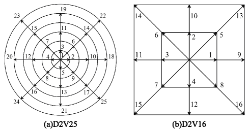
Figure 2: Schematics of two kinds of discrete velocity models used in the present paper. (a)D2V25, (b)D2V16. The numbers in the figures represent the index of discrete velocities.

In this paper, the first-order forward Euler finite difference scheme and the second-order non-oscillatory nonfree dissipative (NND) scheme are used to discrete spatial and temporary derivatives in Eq. (3) and Eq. (13), respectively. The second-order central difference scheme is used to discretize the space derivative in Eq. (14). Two two-dimensional DVMs are adopted in this paper. The DVM used to simulate the benchmark problems has $25$ discrete velocities as shown in Fig. 3(a), and the DVM used to simulate the RMI has $16$ discrete velocities as shown in Fig. 3(b).

The mathematical expressions of these two kinds of DVM are as follows,

$$\text{D2V25}:$$ (28)

$$({v_{ix}},{v_{iy}})=\left\{\begin{array}[]{l}0,\qquad\qquad\qquad\qquad\qquad\qquad i=1,\\ c[\cos\frac{{(i-2)\pi}}{2},\sin\frac{{(i-2)\pi}}{2}],{\rm{\qquad}}i=2-5,\\ 2c[\cos\frac{{(2i-3)\pi}}{4},\sin\frac{{(2i-3)\pi}}{4}],{\rm{\quad}}i=6-9,\\ 3c[\cos\frac{{(i-10)\pi}}{2},\sin\frac{{(i-10)\pi}}{2}],{\rm{}}i=10-13,\\ 4c[\cos\frac{{(2i-11)\pi}}{4},\sin\frac{{(2i-11)\pi}}{4}],{\rm{}}i=14-17,\\ 5c[\cos\frac{{(i-18)\pi}}{2},\sin\frac{{(i-18)\pi}}{2}],{\rm{}}i=18-21,\\ 6c[\cos\frac{{(2i-19)\pi}}{4},\sin\frac{{(2i-19)\pi}}{4}],{\rm{}}i=22-25,\end{array}\right.$$ (36)

$$\text{D2V16}:\left({{v_{ix}},{v_{iy}}}\right)=\left\{\begin{array}[]{l}cyc:c\left({\pm 1,0}\right){\rm{,\quad\quad\;1}}\leq i\leq 4,\\ c\left({\pm 1,\pm 1}\right){\rm{,\quad\quad\quad\quad 1}}\leq i\leq 8,\\ cyc:2c\left({\pm 1,0}\right){\rm{,\quad\quad 9}}\leq i\leq 12,\\ 2c\left({\pm 1,\pm 1}\right){\rm{,\quad\quad\quad\;\;13}}\leq i\leq 16,\end{array}\right.$$ (41)

where ‘cyc’ represents the indicates cyclic permutation. $c$ is a free parameter to optimize the properties of the DVM.

It should be noted that, in standard Lattice Boltzmann Method (LBM), the image of “propagation + collision” is used, and the direction of discrete velocity actually represents the motion direction of particles. Succi (2001) In DBM, although the discrete velocity is still used, the image of “propagation + collision” no longer exists, and the function of DVM is to ensure that the physical constraints described by Eqs. (6) and (7) strictly hold. Xu and Zhang (2022) Therefore, the construction of DVM in DBM is very flexible, which is based on comprehensive consideration of physical symmetry, computational efficiency, etc.

III.2 Non-dimensionalization

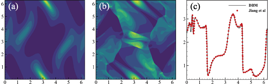
Figure 3: DBM results of Orszag-Tang vortex problem. (a) Pressure contour at time $t=0.5$ of DBM results. (b) Pressure contour at time $t=3$ of DBM results. (c) Pressure distributions along $y=0.625\pi$ at $t=3$. The solid line represent the DBM result while the red dots represent the result of Jiang and Wu (1999).

In this work, the physical quantities used are all non-dimensionalized. The reference density $n_{0}$, tempure $T_{0}$, and length $L_{0}$ are used to make dimensionlessness as

$$\hat{\rho}=\frac{\rho}{{{\rho_{0}}}},\quad\hat{T}=\frac{T}{{{T_{0}}}},\quad\left({\hat{t},\hat{\tau}}\right)=\frac{{\left({t,\tau}\right)}}{{L_{0}/\sqrt{R{T_{0}}}}},\quad{\hat{r}_{\alpha}}=\frac{{{r_{\alpha}}}}{{{L_{0}}}},$$

$$\hat{P}=\frac{P}{{{\rho_{0}}{R}T_{0}}},\quad\left({\hat{f},{{\hat{f}}^{eq}},{{\hat{f}}_{i}},\hat{f}_{i}^{eq}}\right)=\frac{{\left({f,{f^{eq}},{f_{i}},f_{i}^{eq}}\right)}}{{{\rho_{0}}{{\left({R{L_{0}}}\right)}^{-1}}}},$$

$$\left({{{\hat{v}}_{\alpha}},{{\hat{c}}_{\alpha}},{{\hat{u}}_{\alpha}}}\right)=\frac{{\left({{v_{\alpha}},{c_{\alpha}},{u_{\alpha}}}\right)}}{{{\sqrt{R{T_{0}}}}}},\quad\hat{B}=\frac{{B{L_{0}}}}{{{t_{0}}}}\sqrt{{\mu_{0}}{\rho_{0}}},$$

$$\hat{\kappa}=\frac{\kappa}{{{\rho_{0}}R{L_{0}}\sqrt{R{T_{0}}}}},\quad\hat{\mu}=\frac{\mu}{{{\rho_{0}}{L_{0}}\sqrt{R{T_{0}}}}},$$

where $\kappa$ and $\mu$ are the heat conduction and viscosity coefficient, respectively. The variables on the left with “$\land$” represent dimensionless variables, and the variables on the right hand without “$\land$” represent dimensional variables. In the following, to be simplified, the “$\land$” of dimensionless variables are all omitted.

The $Kn$ in BGK model is defined as,Xu and Zhang (2022)

$$Kn=\frac{{{\lambda_{BGK}}}}{L}=\frac{\tau}{L}\sqrt{\frac{{8RT}}{\pi}}=\frac{{\hat{\tau}}}{{\hat{L}}}\sqrt{\frac{{8\hat{T}}}{\pi}},$$ (42)

where $\hat{L}$ is the nondimensional characteristic length scale.

III.3 Orszag-Vortex problem

This problem is first proposed by Orszag and Tang in 1979.(Orszag and Tang, 1979) Due to the complex vortex and shock wave structures generated during evolution, this problem has been widely used to demonstrate the validity of new models. Here, the initial configuration and conditions are identical to Jiang and Wu (1999), as follows,

$$\begin{array}[]{l}\rho\left({x,y,0}\right)={\gamma^{2}},\qquad\qquad\qquad{\rm{}}{v_{x}}\left({x,y,0}\right)=-\sin y,{\rm{}}\\ {v_{y}}\left({x,y,0}\right)=\sin x,\qquad\qquad\quad{\rm{}}p\left({x,y,0}\right)=\gamma,\\ {B_{x}}\left({x,y,0}\right)=-\sin y,\qquad\qquad{\rm{}}{B_{y}}\left({x,y,0}\right)=\sin 2x,\end{array}$$ (46)

where $\gamma$ is equal to $5/3$. The computational domain is $\left[{0,2\pi}\right]\times\left[{0,2\pi}\right]$, which has been divided into $N_{x}\times N_{y}=400\times 400$ mesh-cells. The D2V25 model in Fig. 1 is used to discretize the velocity space, where $c=0.6$, ${\eta_{0}}=0.4$ for $i=2,\cdots,5$, ${\eta_{0}}=0.8$ for $i=6,\cdots,9$ and ${\eta_{0}}=0$ for others. The time step is $\Delta t=5\times{10^{-4}}$, the space step is $\Delta x=\Delta y=5\times{10^{-3}}\pi$, the relaxation time is $\tau=1\times{10^{-3}}$, and the number of extra degree of freedom is $n=1$. Moreover, the periodic boundaries are applied in both $x$ and $y$ direction.

Figure 3 shows the results calculated by DBM. From Fig. 3(b), it is observed that the system is very complex, forming a variety of vortex and shock wave structures, especially in the center of the flow field. By comparing the DBM results in Figs. 3(a)-(b) with the MHD results in Figs. (12)-(14) given in Jiang and Wu (1999) , it is found that the two sets of results are in good agreement. For quantitative comparison, the pressure distribution along $y=0.625\pi$ at time $t=3$ is extracted and plotted together with the result of Jiang and Wu (1999) in Fig. 3(c). It can be seen that the DBM results from $x=0.2$ to $x=0.4$ is slightly lower, while the rest of results is in good agreement with those of Jiang and Wu (1999), which proves the validity of the new magnetohydrodynamic DBM. In fact, the kinetics behavior of OT turbulence evolution is far from well studied. In addition to the comparison of the above HNE characteristics, the TNE characteristics are further extracted and plotted in Fig. 4.

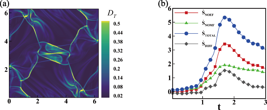
Figure 4: TNE effects of Orszag-Tang vortex problem. (a) Contour of total TNE strength $D_{T}$ at $t=3$, (b) evolution of three kinds of entropy production rate with time. The red line with square symbol corresponding to ${{\dot{S}}_{NOEF}}$. The green line with delta symbol corresponding to ${{\dot{S}}_{NOMF}}$. The blue line with circle symbol corresponding to the total entropy production rate. The gray line with diamond symbol corresponding to the difference between ${{\dot{S}}_{NOEF}}$ and ${{\dot{S}}_{NOMF}}$.

Figure 4(a) shows the contour map of total TNE strength ${D_{T}}$ at $t=3$. It is found that the TNE effects are most pronounced in the shock front where high physical gradients exist. For the rest of the flows field, the TNE strength is weak, indicating that the system is close to the local thermodynamic equilibrium state. Figure 4(b) shows the evolution of four kinds of entropy production rates with time. It can be seen that, both the four kinds of entropy production rates show two stages effect: before $t=1.7$, the entropy production rates keep increasing with time; After $t=1.7$, the entropy production rates reach the peak value and then keep decreasing with time. In fact, there is a positive correlation between the entropy production rate and the physical quantity gradient. Before $t=1.7$, the evolution of flow field is in dominated and the velocity and temperature gradients keep increasing, which leads to the increase of entropy production rates. After $t=1.7$, the dissipative effects are in dominated, resulting in the reduction of gradients and entropy production rates. Besides, in the early stage, it is found that the ${{\dot{S}}_{NOEF}}$ increases from $0$, while the ${{\dot{S}}_{NOMF}}$ increases from about $0.1$. This is because the initial temperature field is uniform and there exists no temperature gradient. For the initial velocity field, the initial velocity gradient induces a momentum exchange and leads to an initial entropy production rate ${{\dot{S}}_{NOMF}}$. Besides, as the flow field develops, the entropy production rate ${{\dot{S}}_{NOEF}}$ exceeds ${{\dot{S}}_{NOMF}}$ after $t=1$ and is always larger than ${{\dot{S}}_{NOMF}}$ in the subsequent evolution, indicating that the entropy production caused by NOEF is in dominant in the late stage of OT vortex problem.

From the perspective of compression science, generally, the increase of entropy production rate predicts the increase of compression difficulty. In the process of OT evolution, the difficulty of compression is divided into stages: in the first stage, the difficulty of compression increases with time; in the second stage, the difficulty of compression decreases with time.

IV Richtmyer-Meshkov instability

In this section, the RMI induced by a shock wave passing through a heavy/light density interface is simulated by using the current DBM. The effects of different initial magnetic field ${B_{0}}$ on the evolution of RMI and the subsequent re-shock process, both the induced HNE and TNE effects, are carefully investigated. This section consists of three subsections. In the first subsection, the initial configuration of RMI is given. In the next subsection, the HNE and TNE effects of RMI without magnetic field are investigated. In the last subsection, the HNE and TNE effects of RMI with different initial magnetic field are carefully investigated. Meanwhile, the entropy production rates under different initial magnetic field are calculated and analyzed. As a preliminary application of related research work, this work adopts a first-order model. The reason is as follows: (i) in the case of low-intensity shocks, the first-order model is sufficient, (ii) the results of these low-level models provide a technical and cognitive basis for the next step of higher intensity shock scenarios.

IV.1 Flow field Settings

Figure 5 shows the initial flow field of RMI. The length and height of the two-dimension computation domain are 20 and 80, respectively. The computation domain is divided into $N_{x}\times N_{y}=200\times 800$ mesh-cells. Initially, a sinusoidal perturbation interface is located at $y=3N_{y}/4$, with wavelength $\lambda=d$, where $d=20$ is equal to the length of computation domain. The amplitude is set to be ${y_{0}}=0.1d$, which corresponds to a small perturbation case. The initial shock wave is located at $y=7N_{y}/8$, with the physical quantities on the left and right sides of the shock wave connected by the Rankine–Hugoniot conditions. Thus, the shock wave and perturbed interface separate the domain into three regions as ${S_{1}}$, ${S_{2}}$, and ${S_{3}}$. ${S_{1}}$ is the area that has been compressed by the passed shock wave. ${S_{2}}$ is the region with high density and ${S_{3}}$ is the region with light density. Furthermore, the periodic boundary conditions are applied to the boundaries in $x$ direction, and the free inflow and solid boundary condition are applied to the boundaries at the top and bottom of $y$ direction, respectively. The initial hydrodynamic quantities are as follows,

$$\left\{\begin{array}[]{l}{\left({\rho,{u_{x}},{u_{y}},p}\right)_{S1}}=\left({3.1304,0,-0.28005,2.1187}\right)\\ {\left({\rho,{u_{x}},{u_{y}},p}\right)_{S2}}=\left({2.3333,0,0,1.4}\right)\\ {\left({\rho,{u_{x}},{u_{y}},p}\right)_{S3}}=\left({1,0,0,1.4}\right)\end{array}\right..$$ (50)

With the above initial quantities, a shock wave with $\rm{Ma}=1.2$ is formed to impact the sinusoidal perturbation interface. The Atwood number is $\rm{At}=0.4$. The D2V16 model in Fig. 2 is adopted to discrete the particle velocity space, and the parameters are $c=1$, ${\eta_{0}}=5$ for $i=1,\cdots,4$ and ${\eta_{0}}=0$ for others. The other parameters of DBM are as follows: space step $\Delta x=\Delta y=1\times{10^{-1}}$, time step $\Delta t=1\times{10^{-3}}$, relaxation time $\tau=1\times{10^{-3}}$ and the number of extra degrees of freedom $n=3$, i.e., the specific heat ratio $\gamma=1.4$. The maximum initial CFL number is

$${C_{0}}=\frac{{\max\left({\left|{{u_{y}}}\right|+{c_{\max}}}\right)\cdot\Delta t}}{{\Delta x}}=0.0228,$$ (51)

where ${c_{\max}}=2$ is the maximum velocity in DVM.

IV.2 Grid convergence test

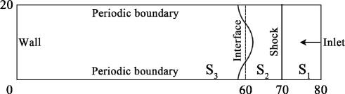
Figure 5: Schematic of initial configuration of Richtmyer-Meshkov instability.

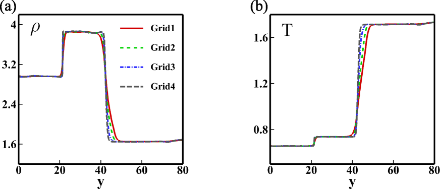
Figure 6: Distribution of physical quantities along $x=10$ of four kinds of grid at $t=100$. (a)Density, (b)Temperature.

In order to verify the effectiveness of numerical resolution, a grid convergence test is performed. Four kinds of grid numbers are selected as Grid1: $N_{x}\times N_{y}=50\times 200$, Grid2: $N_{x}\times N_{y}=100\times 400$, Grid3: $N_{x}\times N_{y}=200\times 800$ and Grid4: $N_{x}\times N_{y}=400\times 1600$. The corresponding space steps are $\Delta x=\Delta y=4\times{10^{-1}}$, $\Delta x=\Delta y=2\times{10^{-1}}$, $\Delta x=\Delta y=1\times{10^{-1}}$, $\Delta x=\Delta y=5\times{10^{-2}}$, respectively. The other calculation parameter settings of DBM are: time step $\Delta t=1\times{10^{-1}}$, relaxation time $\tau=1\times{10^{-3}}$ and the number of extra degrees of freedom $n=3$, i.e., the specific heat ratio $\gamma=1.4$. Figure 6 shows the distribution of density and temperature along $x=10$. It can be seen that the results of $200\times 800$ and $400\times 1600$ meshes are quite identical. By comprehensively considering numerical resolution and computational cost, the $200\times 800$ meshed are selected for calculation and analysis in this paper.

IV.3 RMI without magnetic field

In this section, the HNE and TNE effects of RMI without magnetic field are investigated. The magnetic field strength $B_{0}=0.0$, and the other parameters are consistent with those in Sec. IV.1.

IV.3.1 HNE characteristics

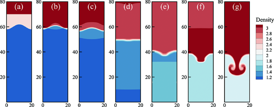
Figure 7: Density contours in the evolution of RMI without initial applied magnetic field at different times: (a)$t=0$, (b)$t=10$, (c)$t=15$, (d)$t=40$, (e)$t=70$, (f)$t=100$, (g)$t=250$.

Figure 7 shows the density evolution in RMI via snapshots at times $t=0$,$10$,$15$,$40$,$70$,$100$,$250$. At $t=10$, the shock wave hits the interface and interacts with the interface. At $t=15$, the shock wave passes through the interface, forming a reflected rarefaction wave propagating upward to top boundary and a transmission shock wave propagating downward to the bottom boundary. Meanwhile, the perturbation amplitude gradually decreases to zero with the motion of interface. Then, the interface reverses and the perturbation amplitude grows again, accompanied by the reversal of the initial perturbation interface peak and valley. At $t=40$, the transmission shock wave moves to the bottom solid wall and reflects. At $t=70$, the reflected transmission shock wave passes through the interface again, forming a reflected rarefaction wave to light fluids and a transmission shock wave to heavy fluids. Under the action of the secondary shock (reflected transmission shock wave), the speed of interface development is greatly accelerated and the speed difference on both sides of the interface increases rapidly. Then, the Kelvin-Helmholtz instability (KHI) appears at the head of the spike, eventually forming a mushroom-like structure. During the interface evolution, the light and heavy fluids continuously mix with each other.

IV.3.2 TNE effects

Figure 8(a) shows the global average TNE strength ${\bar{D}_{T}}$, NOMF ${\bar{D}_{2}}$, NOEF ${\bar{D}_{3,1}}$, the flux of NOMF ${\bar{D}_{3}}$ and the flux of NOEF ${\bar{D}_{4,2}}$ from $t=0$ to $t=500$. It can be found that the strength of ${\bar{D}_{2}}$ is much lower than other TNE effects, and the trend of ${\bar{D}_{T}}$ is basically the same as that of ${\bar{D}_{3,1}}$, which means that the TNE effects of the whole system caused by viscosity are weaker than the TNE effects caused by heat conduction. The TNE strength ${\bar{D}_{T}}$ of the system basically increases with time before about $t=320$, while decreases with time after $t=320$. In fact, there exists two competition mechanisms. Before $t=320$, the evolution of RMI is located at linear and weak nonlinear development stage. With the development of the interface, the physical quantities gradient near the interface increases rapidly, and the non-equilibrium region augments, which cause the increasing of ${\bar{D}_{T}}$. After $t=320$, the evolution of RMI is located at the late stage of nonlinear development. At this time, the dissipation effects such as viscosity and heat conduction are dominant, which increase the degree of mixing near the interface and reduce the gradient of physical quantities, causing the decrease of ${\bar{D}_{T}}$. Besides, from the red line $({\bar{D}_{T}})$, three key time points are marked, which are shown in the enlarged picture Fig. 8(b).

Figure 8: Contours of global average TNE quantities ${\bar{D}_{T}}$, ${\bar{D}_{2}}$, ${\bar{D}_{3}}$, ${\bar{D}_{3,1}}$ and ${\bar{D}_{4,2}}.$ (a) The time ranges from $t=0$ to $t=500$, (b) the time ranges from $t=0$ to $t=100$.

Figure 8(b) shows the the global average TNE strength ${\bar{D}_{T}}$, NOMF ${\bar{D}_{2}}$, NOEF ${\bar{D}_{3,1}}$ and the flux of NOEF ${\bar{D}_{4,2}}$ from $t=0$ to $t=100$. It is found that, before time point 1, TNE effects decrease very slowly with time due to dissipation effects. At time point 1, the shock wave passes through the interface, causing the distribution function near the interface to deviate greatly from the local thermodynamic equilibrium state. After time point 1, the dissipative effects tend to reduce TNE effects, while the high $Kn$ makes it difficult to recover to the local thermodynamic equilibrium state, causing the increase of all TNE effects. At time point 2, the transmission shock wave hits the boundary and reflects. In this process, the gradients of macroscopic physical quantities change, resulting in the fluctuation of TNE quantities. At time point 3, the reflected transmission shock wave hits the interface again. Since the direction of the shock wave is opposite to that of the first time, not all TNE quantities increase. The flux of NOEF, i.e., ${\bar{D}_{4,2}}$ decreases, while the rest of the TNE quantities increase. Because the interface has reversed when the shock wave hits the interface for the second time, the vorticity generated is further deposited at the interface after time point 3, which leads to the accelerated development of the interface, the expansion of the non-equilibrium area and the continuous increase of all TNE quantities.

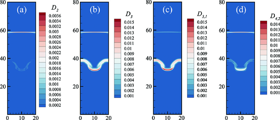
Figure 9: Contours of different TNE quantities of RMI at $t=100$. (a)$D_{2}$, (b)$D_{3}$, (c)$D_{3,1}$, (d)$D_{4,2}$

Figure 9 shows the contours of TNE quantities $D_{2}$, $D_{3}$, $D_{3,1}$, $D_{4,2}$ at $t=100$, at which time the reflected transmission shock wave has passed the perturbed interface. From Fig. 9(a), it is found that $D_{2}$ mainly distributed at shock wavefront and the perturbed interface, and the intensity at the shock wavefront is much higher than that at the perturbed interface. For the rest of the flow field, the $D_{2}$ is almost zero. Therefore, $D_{2}$ can be used to capture the location of shock wave during RMI. Due to the strong momentum transport and shear effects caused by the large density and velocity gradient, the $D_{2}$ is most remarkable at shock wavefront. Figure 9(c) shows the distribution of $D_{3,1}$. It reaches the maximum value at perturbed interface. Thus, $D_{3,1}$ can be used to capture the evolution of interface and the amplitude. In this case, the temperature gradient near perturbed interface is bigger than that near shock wavefront, causing strong energy transport. Thus, the $D_{3,1}$ is most remarkable at perturbed interface. Though $D_{2}$ and $D_{3,1}$ can be used to identify the shock wavefront and perturbed interface respectively, they cannot be used to identify both of them. Compared with $D_{2}$ and $D_{3,1}$, $D_{3}$ and $D_{4,2}$ are more suitable. $D_{3}$ provides the most distinguishable interfaces, which is also proved by Zhang et al. (2019b). During the evolution of RMI, both of these four TNE quantities can be used as the supplement of the macroscopic quantities contours of flow field.

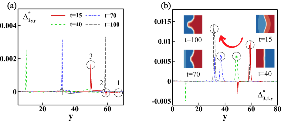
Figure 10: Distribution of different TNE quantities along $N_{x}/2$ at $t=15$, $t=40$, $t=70$ and $t=100$. (a)$\Delta_{2yy}^{*}$, (b)$\Delta_{3,1y}^{*}$.

In order to investigate the evolution of non-equilibrium effects with time for a more detailed analysis, the axes $x=N_{x}/2$ is selected and observed to see how the distribution of TNE quantities on the axes evolve over time. Figure 10(a) shows the distribution of the component $\Delta_{2yy}^{*}$ of NOMF $\bm{\Delta}_{2}^{*}$. It can be seen from the red line that $\Delta_{2yy}^{*}$ mainly distributes in three areas marked with "1", "2", "3" from right to left, which exactly corresponding to rarefaction, material interface and transmission shock wave. Besides, the strength of $\Delta_{2yy}^{*}$ near material interface is stronger than rarefaction but weaker than transmission shock wave. With time evolution, the intensity of $\Delta_{2yy}^{*}$ near interface gradually decreases, but the intensity of $\Delta_{2yy}^{*}$ near transmission shock wave gradually increases. Figure 10(b) shows the distribution of the component $\Delta_{3,1y}^{*}$ of NOEF $\bm{\Delta}_{3,1}^{*}$. It can be seen from the red line that the strength of $\Delta_{3,1y}^{*}$ near material interface is much stronger than that near transmission shock wave. After the reflection of transmission shock wave, the direction of $\Delta_{3,1y}^{*}$ reverses, which is different from $\Delta_{2yy}^{*}$. By further observing the distribution of $\Delta_{3,1y}^{*}$ near material interface, it is found that the intensity of $\Delta_{3,1y}^{*}$ first decreases then increases. The decreasing of $\Delta_{3,1y}^{*}$ is mainly due to the increase of mixing area near interface, where the gradients of physical quantities decrease. The increasing of $\Delta_{3,1y}^{*}$ is due to the passing of secondary shock, where the energy is transported from shock to material interface. Besides, there exists double-peak structure near material interface. In this case, the $\Delta_{3,1y}^{*}$ first gets its maximum value at the right peak then the left one. The shift of the maximum peak depends on the direction of shock wave.

IV.4 RMI with magnetic field

The magnetic field can suppress the evolution of RMI through transporting the barochorically generated vorticity away from the interface (Samtaney, 2003; Sano, Inoue, and Nishihara, 2013). In this section, the effects of magnetic fields on the evolution of RMI, including HNE and TNE effects, are analyzed. The initial magnetic field is set on the $y$ direction, and the parameters setting in different cases are shown in Table 1, where $\beta=2p_{0}/B_{0}^{2}$ is the nondimensional strength of the magnetic field. Samtaney (2003) The other parameters are consistent with those in Sec. IV.1.

Table 1: Settings for RMI with different initial applied magnetic fields.

Cases	$B_{0}$	$\beta$	Cases	$B_{0}$	$\beta$
Case I	0.01	$2.80\times 10^{4}$	Case VI	0.10	$280.0$
Case II	0.02	$7.00\times 10^{3}$	Case VII	0.15	$124.4$
Case III	0.03	$3.11\times 10^{3}$	Case VIII	0.20	$70.0$
Case IV	0.04	$1.75\times 10^{3}$	Case IX	0.25	$44.8$
Case V	0.05	$1.12\times 10^{3}$	Case X	0.30	$31.1$

IV.4.1 HNE characteristics

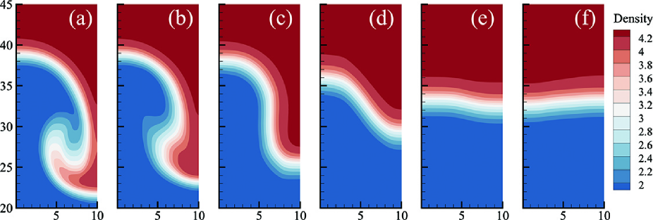
Figure 11: Density contours with different applied magnetic fields at $t=250$. (a)$B_{0}=0.01$, (b)$B_{0}=0.03$, (c)$B_{0}=0.05$, (d)$B_{0}=0.10$, (e)$B_{0}=0.20$, (f)$B_{0}=0.30$

Figure 11 shows the density contours of different initial magnetic fields range from $0.01$ to $0.30$ at $t=250$. It is found that the evolution of interface is gradually suppressed with the increase of magnetic fields. For the case of $B_{0}=0.01$, the Kelvin-Helmholtz instability (KHI) is still developed and observed, forming the "mushroom-like" structure. For the case of $B_{0}=0.03$ and $B_{0}=0.05$, the KHI degenerates and the amplitude of interface decreases. From figures 11 (a)-(e), it can be observed that the interface can still reverse. However, from Fig. 11 (f), it is observed that the interface no longer reverses for the case $B_{0}=0.30$, indicating that there exists a critical magnetic field $B_{0,C}$ under which the amplitude of interface can be suppressed to $0$.

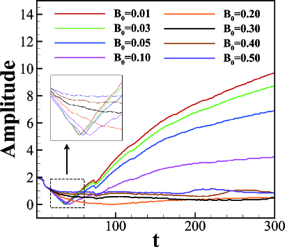
Figure 12: Evolution of amplitude of RMI with different initial applied magnetic fields from $t=0$ to $t=200$.

Figure 12 further shows the evolution of interface amplitude with time under initial applied different magnetic fields. Obviously, the magnetic fields delay the time interface inverse. For the cases ($B_{0}\leq 0.05$), the magnetic fields have little effect on the flow field before inverse but can significantly inhibit the development of interface amplitude after inverse. With the increase of the magnetic fields, the influence of the secondary shock on the perturbation amplitude is weakened. This is mainly because the magnetic field inhibits the development of the interface, which reduces the perturbation amplitude when the secondary shock passing through interface. Thus, the induced vorticity reduces. With the increase of magnetic fields, a critical situation appears where the perturbation is nearly inhibited and the amplitude no longer increases. As the magnetic field further increase, the interface no longer reverse, and the vorticity induced by secondary shock will prevent the development of interface. When magnetic field exceeds the critical magnetic field, the stronger the magnetic field, the closer the interface shape is to the initial state.

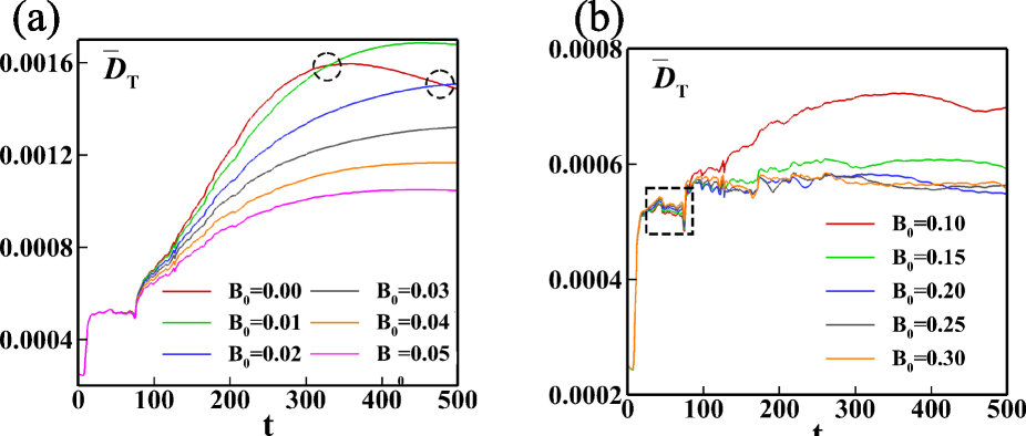
Figure 13: Evolution of global average TNE effects with different initial applied magnetic fields from $t=0$ to $t=500$.

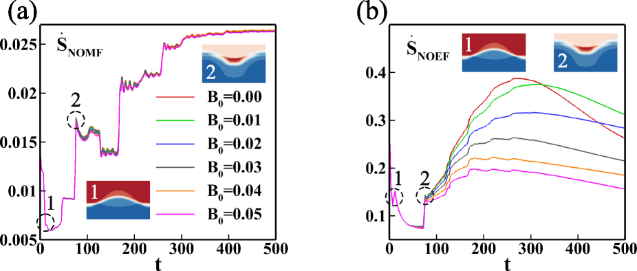
Figure 14: Evolution of entropy production rates from $t=0$ to $t=500$ with magnetic fields range from $0.01$ to $0.05$.

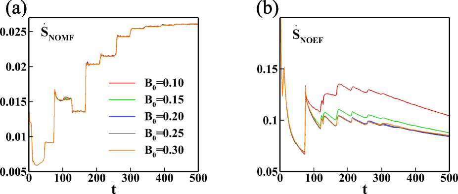
Figure 15: Evolution of entropy production rates from $t=0$ to $t=500$ with magnetic fields range from $0.10$ to $0.30$.

IV.4.2 TNE effects

Figure 13(a) shows the global average TNE strength $\bar{D}_{T}$ with different initial magnetic fields range from $0.00$ to $0.05$. It is observed that, before the secondary shock, the increase of magnetic fields shows little effect to $\bar{D}_{T}$. After secondary shock, $\bar{D}_{T}$ quickly increases with the evolution of interface, and the magnetic fields show greatly effects for suppressing $\bar{D}_{T}$. However, it is found that $\bar{D}_{T}$ for the case of $B_{0}=0.01$ and $B_{0}=0.02$ are greater than that of $B_{0}=0.00$ after time marked with circle. This is because the magnetic fields suppress the shear effects around interface, thus delay the time KHI arises and decrease the strength of KHI. The emergence and development of KHI can enhance mixing and reduce the gradients of physical quantities, which is helpful for reducing $\bar{D}_{T}$. The inflection point of TNE intensity can be regarded as the criterion to judge whether KHI is fully developed. Before the inflection point, the development of perturbation amplitude dominates and the TNE is enhanced; after the inflection point, the fully development of KHI results in the enhancement of dissipation effect and the decrease of TNE intensity.

Figure 13(b) shows the global average TNE strength $\bar{D}_{T}$ with different initial magnetic fields range from $0.10$ to $0.30$. It is found that the influence of magnetic field for TNE could be divided into two stages. Before the inverse of interface, as the strength of magnetic field increases, the TNE strength slightly increases. After the inverse of interface, the TNE strength decreases significantly with the increase of magnetic field strength. In fact, the magnetic field consistently inhibits the interface development during the RMI evolution. Before the interface inverse, the magnetic field inhibits the interface inverse, indirectly enhancing the physical quantity gradient near the interface, resulting in the enhancement of TNE intensity. After the interface inverse, the magnetic field inhibits the shear effect near the interface, as has been explained before. From Fig. 13(b), it can also be found that after secondary, $\bar{D}_{T}$ keeps decreasing with the increase of magnetic fields, and there exists a critical magnetic field, above which $\bar{D}_{T}$ no longer decreases. Thus, the magnetic field intensity $B_{0,C}$, corresponding to the minimum value $\bar{D}_{T,min}$ of global average TNE intensity just after the reshock stage, can be used as the critical magnetic field intensity to inhibit the development of RMI interface.

IV.4.3 Entropy production

Figure 14 shows the two parts of entropy production rate ${{\dot{S}}_{NOMF}}$ and ${{\dot{S}}_{NOEF}}$ of the global system with magnetic fields range from $0.01$ to $0.05$. From Fig. 14(a) we can find that the entropy production rate ${{\dot{S}}_{NOMF}}$ shows stages. Before the shock wave contact the perturbed interface, the rate sharply decreased. Then, after the shock wave contacts the solid wall and passed through interface again, the rate appears two jumps. After re-shock, the rate first decreases and then increases to the maximum. With the increase of magnetic fields, the values of ${{\dot{S}}_{NOMF}}$ are basically the same. From Fig. 14(b), it is observed that when the shock first contacts the interface, the entropy production rate ${{\dot{S}}_{NOEF}}$ suddenly increases, as shown by point ‘1’, which is different from ${{\dot{S}}_{NOMF}}$. It means that the shock wave enhances physical quantity gradients near interface. When the transmitted shock wave passes interface again, as shown by point ‘2’, the rate increases greatly, which is also observed from ${{\dot{S}}_{NOMF}}$. After re-shock, the rate first gradually increases and then decreases, which can be divided into two stages. When the initial magnetic field strength gradually increases, the ${{\dot{S}}_{NOEF}}$ also shows no difference before re-shock, but is greatly reduced after re-shock. In general, the ${{\dot{S}}_{NOEF}}$ contributes more to entropy increase than ${{\dot{S}}_{NOMF}}$, but the strength of ${{\dot{S}}_{NOEF}}$ could be greatly inhibited by adding magnetic field.

Figure 15 shows the two parts of entropy production rate ${{\dot{S}}_{NOMF}}$ and ${{\dot{S}}_{NOEF}}$ of the global system with magnetic fields range from $0.10$ to $0.30$. From Fig. 14(a) and Fig. 15(a), it can observed that the fluctuations in the ${{\dot{S}}_{NOMF}}$ curve have been smoothed due to the increase of magnetic fields. Different from ${{\dot{S}}_{NOMF}}$, the evolution of ${{\dot{S}}_{NOEF}}$ is strongly affected by magnetic fields. With the increase of magnetic fields, the evolution of ${{\dot{S}}_{NOEF}}$ after re-shock is significantly inhibited. It can be observed that there exists a critical magnetic field, under which the ${{\dot{S}}_{NOEF}}$ no longer decreases.

V Conclusion and discussion

When the particle collision frequency is sufficiently high, the kinetic behaviors can be described by the reduced hydrodynamic equations. When the particle collision frequency is negligibly small, the kinetic behaviors can be described by the reduced Vlasov equation where the collision effect is completely ignored. The situation between the two extreme cases is generally difficult to treat with and consequently poorly understood, which is responsible for the fact that the kinetic effects caused by particle collision in ICF are still far from clear understanding although they have potential impact on ICF ignition.

To attack the problem, the preferred method/model needs to have simultaneously two physical functions. First, it can construct physical model that present numerical data to recover the HNE and TNE behaviors we aim to investigate before simulation. Second, it can present methods for checking the non-equilibrium state, describing and analyzing the resulting effects from massive data after simulation. In the DBM, for the first physical function, the model equations are composed of a discrete Boltzmann equation coupled by a magnetic induction equation. For the second physical function, DBM intrinsically includes some schemes for studying the TNE behaviors. The most fundamental one is to use the non-conserved kinetic moments of $(f-f^{eq})$ to check the TNE state and describe the TNE behaviors. The phase space description method based on the non-conserved kinetic moments of $(f-f^{eq})$ presents an intuitive geometrical correspondence for the complicated TNE state and behaviors, which is important for the deep investigation and clear understanding. The first function is verified by recovering HNE behaviors of a number of typical benchmark problems including sod shock tube, thermal couette flow and OT vortex problem. Besides, the most relevant TNE behaviors of OT vortex problem are investigated for the first time. As a further application, the kinetic study on RMI system with initial horizontal magnetic field is performed. Physical findings are as below: (i) Generally, the entropy production rate is in positive correlation to the difficulty of compression. During the evolution of OT system, the stage behavior of entropy production rate, first increases then decreases with time, shows the same stage behavior of compression difficulty. (ii) In the case without external magnetic field, the NOMF gets its maximum value near the shock front, while the NOEF gets its maximum value near the perturbed interface. During the perturbed interface inverse process of RMI, the NOEF along the central axis shows two-peak values near perturbed interface, and the impact of shock wave significantly enhances the NOEF. (iii) In the case with external magnetic field, the magnetic field shows inhibitory effects on the evolution of RMI. Specifically, the magnetic field has a pronounced inhibitory effect on the nonlinear stage, especially on the generation of KHI. Besides, there exists a critical magnetic field under which the amplitude of interface can be suppressed to $0$. (iv) Before the interface inverse, the magnetic field indirectly enhances the TNE intensity by suppressing the interface inverse. After the interface inverse, the magnetic field significantly suppresses the TNE intensity by inhibiting the further development of the perturbed interface. (v) In terms of entropy production rate, the magnetic field has pronounced inhibitory effect on the entropy production rate caused by heat conduction, but has a weak effect on the entropy production rate caused by viscosity.

Potential applications of above physical findings are as follows: (i) Based on features of NOMF and NOEF, shock front and perturbed interface during RMI evolution can be physically captured in the numerical experiments. (ii) The magnetic field intensity $B_{0,C}$, corresponding to the minimum value $\bar{D}_{T,min}$ of global average TNE intensity just after the re-shock stage, can be used as the critical magnetic field intensity to inhibit the development of RMI interface. (iii) From the perspective of entropy production rate, the magnetic field intensity $B_{0,C}$, corresponding to the minimum value of entropy production rate caused by heat conduction just after the re-shock stage, plays the same role. The future work includes two-fluid DBM where the ion and electrons are considered separately and Prantl number adjustable plasma DBM, etc.

Data Availability Statement

The data that support the findings of this study are available from the corresponding authors upon reasonable request.

Appendix A Kinetic moments used to characterize the first-order and second-order TNE effects

Here, the kinetic moments used to characterize the first-order and second-order TNE effects are given as below,

$$M_{0}^{eq}=\sum\limits_{i}{f_{i}^{eq}}=\rho,$$ (52)

$$M_{1,x}^{eq}=\sum\limits_{i}{f_{i}^{eq}{v_{ix}}}=\rho{u_{x}},$$ (53)

$$M_{1,y}^{eq}=\sum\limits_{i}{f_{i}^{eq}{v_{iy}}}=\rho{u_{y}},$$ (54)

$$M_{2,0}^{eq} = \sum\limits_{i}{f_{i}^{eq}\left({v_{ix}^{2}+v_{iy}^{2}+\eta_{i}^{2}}\right)}$$ (55)

$$= \rho\left[{\left({n+2}\right)RT+u_{x}^{2}+u_{y}^{2}}\right],$$

$$M_{2,xy}^{eq} = \sum\limits_{i}{f_{i}^{eq}{v_{ix}}{v_{iy}}}=\rho{u_{x}}{u_{y}},$$ (56)

$$M_{2,xx}^{eq} = \sum\limits_{i}{f_{i}^{eq}{v_{ix}}{v_{ix}}}=\rho\left({RT+u_{x}^{2}}\right),$$ (57)

$$M_{2,yy}^{eq} = \sum\limits_{i}{f_{i}^{eq}{v_{iy}}{v_{iy}}}=\rho\left({RT+u_{y}^{2}}\right),$$ (58)

$$M_{3,1,x}^{eq} = \sum\limits_{i}{f_{i}^{eq}\left({v_{ix}^{2}+v_{iy}^{2}+\eta_{i}^{2}}\right){v_{ix}}}$$ (59)

$$= \rho{u_{x}}\left[{\left({n+4}\right)RT+u_{x}^{2}+u_{y}^{2}}\right],$$

$$M_{3,1,y}^{eq} = \sum\limits_{i}{f_{i}^{eq}\left({v_{ix}^{2}+v_{iy}^{2}+\eta_{i}^{2}}\right){v_{iy}}}$$ (60)

$$= \rho{u_{y}}\left[{\left({n+4}\right)RT+u_{x}^{2}+u_{y}^{2}}\right],$$

$$M_{3,xxx}^{eq} = \sum\limits_{i}{f_{i}^{eq}v_{ix}^{3}}=\rho{u_{x}}\left({3RT+u_{x}^{2}}\right),$$ (61)

$$M_{3,yyy}^{eq} = \sum\limits_{i}{f_{i}^{eq}v_{iy}^{3}}=\rho{u_{y}}\left({3RT+u_{y}^{2}}\right),$$ (62)

$$M_{3,xxy}^{eq} = \sum\limits_{i}{f_{i}^{eq}v_{ix}^{2}{v_{iy}}}=\rho{u_{y}}\left({RT+u_{x}^{2}}\right),$$ (63)

$$M_{3,xyy}^{eq} = \sum\limits_{i}{f_{i}^{eq}{v_{ix}}v_{iy}^{2}}=\rho{u_{x}}\left({RT+u_{y}^{2}}\right),$$ (64)

$$M_{4,2,xx}^{eq} = \sum\limits_{i}{f_{i}^{eq}\left({v_{ix}^{2}+v_{iy}^{2}+\eta_{i}^{2}}\right)v_{ix}^{2}}$$ (65)

$$= \rho[(n+4)R^{2}T^{2}+RT\left((n+7)u_{x}^{2}+u_{y}^{2}\right)$$

$$+u_{x}^{2}\left(u_{x}^{2}+u_{y}^{2}\right)],$$

$$M_{4,2,yy}^{eq} = \sum\limits_{i}{f_{i}^{eq}\left({v_{ix}^{2}+v_{iy}^{2}+\eta_{i}^{2}}\right)v_{iy}^{2}}$$ (66)

$$= \rho[(n+4)R^{2}T^{2}+RT\left((n+7)u_{y}^{2}+u_{x}^{2}\right)$$

$$+u_{y}^{2}\left(u_{x}^{2}+u_{y}^{2}\right)],$$

$$M_{4,2,xy}^{eq} = \sum\limits_{i}{f_{i}^{eq}\left({v_{ix}^{2}+v_{iy}^{2}+\eta_{i}^{2}}\right){v_{ix}}}{v_{iy}}$$ (67)

$$= \rho{u_{x}}{u_{y}}\left[{\left({n+6}\right)RT+u_{x}^{2}+u_{y}^{2}}\right],$$

$$M_{4,xxxx}^{eq} = \sum\limits_{i}{f_{i}^{eq}v_{ix}^{4}}=\rho\left(3R^{2}T^{2}+6RTu_{x}^{2}+u_{x}^{4}\right),$$ (68)

$$M_{4,yyyy}^{eq} = \sum\limits_{i}{f_{i}^{eq}v_{iy}^{4}}=\rho\left(3R^{2}T^{2}+6RTu_{y}^{2}+u_{y}^{4}\right),$$ (69)

$$M_{4,xxxy}^{eq} = \sum\limits_{i}{f_{i}^{eq}v_{ix}^{3}v_{iy}}=\rho u_{x}u_{y}\left(3RT+u_{x}^{2}\right),$$ (70)

$$M_{4,xyyy}^{eq} = \sum\limits_{i}{f_{i}^{eq}v_{ix}v_{iy}^{3}}=\rho u_{x}u_{y}\left(3RT+u_{y}^{2}\right),$$ (71)

$$M_{4,xxyy}^{eq} = \sum\limits_{i}{f_{i}^{eq}v_{ix}^{2}v_{iy}^{2}}=\rho\left(RT+u_{x}^{2}\right)\left(RT+u_{y}^{2}\right),$$ (72)

$$M_{5,3,xxx}^{eq} = \sum\limits_{i}{f_{i}^{eq}\left({v_{ix}^{2}+v_{iy}^{2}+\eta_{i}^{2}}\right)v_{ix}^{3}}$$ (73)

$$= \rho u_{x}[3(n+6)R^{2}T^{2}+RT\left((n+11)u_{x}^{2}+3u_{y}^{2}\right)$$

$$+u_{x}^{2}\left(u_{x}^{2}+u_{y}^{2}\right)],$$

$$M_{5,3,yyy}^{eq} = \sum\limits_{i}{f_{i}^{eq}\left({v_{ix}^{2}+v_{iy}^{2}+\eta_{i}^{2}}\right)v_{iy}^{3}}$$ (74)

$$= \rho u_{y}[3(n+6)R^{2}T^{2}+RT\left((n+11)u_{y}^{2}+3u_{x}^{2}\right)$$

$$+u_{y}^{2}\left(u_{x}^{2}+u_{y}^{2}\right)],$$

$$M_{5,3,xxy}^{eq} = \sum\limits_{i}{f_{i}^{eq}\left({v_{ix}^{2}+v_{iy}^{2}+\eta_{i}^{2}}\right)v_{ix}^{2}v_{iy}}$$ (75)

$$= \rho u_{y}[(n+6)R^{2}T^{2}+RT\left((n+9)u_{x}^{2}+u_{y}^{2}\right)$$

$$+u_{x}^{2}\left(u_{x}^{2}+u_{y}^{2}\right)],$$

$$M_{5,3,xyy}^{eq} = \sum\limits_{i}{f_{i}^{eq}\left({v_{ix}^{2}+v_{iy}^{2}+\eta_{i}^{2}}\right)v_{ix}v_{iy}^{2}}$$ (76)

$$= \rho u_{x}[(n+6)R^{2}T^{2}+RT\left((n+9)u_{y}^{2}+u_{x}^{2}\right)$$

$$+u_{y}^{2}\left(u_{x}^{2}+u_{y}^{2}\right)],$$

where $p=\rho RT$ obeys the ideal gas law.

Appendix B Chapman-Enskog multi-scale analysis

Through constructing kinetic moments ${{\bf{M}}_{0}}$, ${{\bf{M}}_{1}}$, and ${{\bf{M}}_{2,0}}$ on both sides of Eq (1), the generalized hydrodynamic equations could be obtained as follows,

$$\frac{{\partial\rho}}{{\partial t}}+\nabla\cdot\left({\rho{\bf{u}}}\right)=0,$$ (77)

$$\frac{{\partial\rho{\bf{u}}}}{{\partial t}}+\nabla\cdot\left({\rho{\bf{uu}}+{{\bm{\Delta}}_{2}}}\right)=\rho\bf{a},$$ (78)

$$\frac{{\partial{E_{T}}}}{{\partial t}}+\nabla\cdot\left[{{E_{T}}{\bf{u}}+{{\bm{\Delta}}_{3,1}}}\right]=\rho\bf{a}\cdot\bf{u},$$ (79)

where ${E_{T}}=\rho e+\rho{u^{2}}/2$ is the total energy, and $e$ is the energy density. ${{\bm{\Delta}}_{2}}$ and ${{\bm{\Delta}}_{3,1}}$ are two non-equilibrium quantities defined by Eq. (18). The relationship between ${{\bm{\Delta}}_{2}}$ (${{\bm{\Delta}}_{3,1}}$) and ${\bm{\Delta}}_{2}^{*}$ (${\bm{\Delta}}_{3,1}^{*}$) are given in reference (Gan et al., 2022) as follows,

$${{\bm{\Delta}}_{2}}={\bm{\Delta}}_{2}^{*},$$ (80)

$${{\bm{\Delta}}_{3,1}}={\bm{\Delta}}_{3,1}^{*}+{\bm{\Delta}}_{2}^{*}\cdot{\bf{u}}.$$ (81)

Here, ${\bm{\Delta}}_{2}^{*}$ is defined as non-organized momentum flux (NOMF) , and ${\bm{\Delta}}_{3,1}^{*}$ is defined as non-organized energy flux (NOEF). Compared with the constitutive of viscous stress and heat flux in NS, Burnett and Super-Burnett equations, ${\bm{\Delta}}_{2}^{*}$ and ${\bm{\Delta}}_{3,1}^{*}$ contain the most complete constitutive information. Thus, ${\bm{\Delta}}_{2}^{*}$ and ${\bm{\Delta}}_{3,1}^{*}$ are also referred to as generalized viscous stress and heat flux. However, the specific forms of ${\bm{\Delta}}_{2}^{*}$ and ${\bm{\Delta}}_{3,1}^{*}$ are basically unknown. To get the specific forms of ${\bm{\Delta}}_{2}^{*}$ and ${\bm{\Delta}}_{3,1}^{*}$, we need to determine the order of $f$ to be retained (or the number of kinetic moments to be preserved) through CE multi-scale analysis. The form of CE multi-scale analysis is as follows,

$$f={f^{(0)}}+Kn{f^{(1)}}+K{n^{2}}{f^{(2)}}+K{n^{3}}{f^{(3)}}+\cdots,$$ (82)

$$\frac{\partial}{{\partial t}}=Kn\frac{\partial}{{\partial{t_{1}}}}+K{n^{2}}\frac{\partial}{{\partial{t_{2}}}}+\cdots,$$ (83)

$$\frac{\partial}{{\partial{\bf{r}}}}=Kn\frac{\partial}{{\partial{{\bf{r}}_{1}}}},$$ (84)

where ${f^{(0)}}={f^{eq}}$. Here, the zero-order expansions of the time and space derivatives $\partial/\partial{t_{0}}$ and $\partial/\partial{\bf{r}_{0}}$ are neglected, for the subscript $0$ represents the scale of system and the internal change of system cannot be observed through system scale. Besides, the time is expanded to the second-order and the space is expanded to the first-order. Through this way, the derived equations are exactly the hydrodynamic equations currently used such as NS and Burnett, etc. Theoretically, it is also optional to expand time to the first-order and expand space to the second-order. As long as the derivation process is correct, the obtained hydrodynamic equations are also correct. Substituting Eqs. (82)-(82) into Eq. (1), and retaining the same order terms of $Kn$ numbers, we get,

$$K{n^{1}}:\frac{{\partial{f^{(0)}}}}{{\partial{t_{1}}}}+\frac{{\partial\left({{f^{(0)}}{\bf{v}}}\right)}}{{\partial{{\bf{r}}_{1}}}}=-\frac{1}{\tau}{f^{(1)}},$$ (85)

$$K{n^{2}}:\frac{{\partial{f^{(0)}}}}{{\partial{t_{2}}}}+\frac{{\partial{f^{(1)}}}}{{\partial{t_{1}}}}+\frac{{\partial\left({{f^{(1)}}{\bf{v}}}\right)}}{{\partial{{\bf{r}}_{1}}}}=-\frac{1}{\tau}{f^{(2)}}.$$ (86)

By taking the ${{\bf{M}}_{0}}$, ${{\bf{M}}_{1}}$, and ${{\bf{M}}_{2,0}}$ moments simultaneously on both sides of Eq. (85) and use the relation ${f^{(1)}}=-\tau\left[{\partial{f^{(0)}}/\partial{t_{1}}+\partial({f^{(0)}}{\bf{v}})/\partial{{\bf{r}}_{1}}}\right]$, the viscous stress and heat flux in NS level can be deduced after performing some mathematical transformations, as follows Gan et al. (2022),

$${\bm{\Delta}}_{2,NS}^{*}={\bm{\Delta}}_{2}^{*(1)}=\int_{-\infty}^{\infty}{{f^{(1)}}{{\bf{v}}^{*}}{{\bf{v}}^{*}}d{\bf{v}}}=-\mu\left[{\left({\nabla{\bf{u}}}\right)+{{\left({\nabla{\bf{u}}}\right)}^{\rm{T}}}}\right],$$ (87)

$${\bm{\Delta}}_{3,1,NS}^{*}={\bm{\Delta}}_{3,1}^{*(1)}=\int_{-\infty}^{\infty}{\frac{1}{2}{f^{(1)}}{{\bf{v}}^{*}}\cdot{{\bf{v}}^{*}}{{\bf{v}}^{*}}d{\bf{v}}}=-\kappa\nabla T,$$ (88)

where $\mu=\tau\rho RT$ is the viscosity coefficient and $\kappa=2\tau\rho RT$ is the heat conductivity. Similarly, the viscous stress ${\bm{\Delta}}_{2}^{*(2)}$ and heat flux ${\bm{\Delta}}_{3,1}^{*(2)}$ contributed by $f^{(2)}$ can be deduced from Eq. (86), and the viscous stress and heat flux in Burnett level are ${\bm{\Delta}}_{2,Burnett}^{*}={\bm{\Delta}}_{2}^{*(1)}+{\bm{\Delta}}_{2}^{*(2)}$ and ${\bm{\Delta}}_{3,1,Burnett}^{*}={\bm{\Delta}}_{3,1}^{*(1)}+{\bm{\Delta}}_{3,1}^{*(2)}$, respectively. It should be noted that, CE gives the dependence of $(n+1)$-th order distribution function $f^{(n+1)}$ on the ${n}$-th order distribution function $f^{(n)}$, and finally gives the dependence of $f^{(n+1)}$ on $f^{(0)}$, where $f^{(0)}$ is the only one whose kinetic moments are known and can be relied upon in the modeling process. In the derivation of the first-order constitutive relations in NS, the highest-order kinetic moment used is ${\bf{M}}_{4,2}$. As for the derivation of the second-order constitutive relations in Burnett, the highest-order kinetic moment used is ${\bf{M}}_{5,3}$.

Appendix C Kinetic Macroscopic Modeling and Kinetic Direct Modeling method

There exist two kinds of methods to obtain the macroscopic hydrodynamic equations. The first is the traditional macroscopic direct modeling method which is based on the continuum assumption and near equilibrium approximation. The second is the Kinetic Macroscopic Modeling (KMM) method, that is, starting from kinetic equations, to derive the corresponding macroscopic hydrodynamic equations via CE multi-scale analysis. Due to different research ideas, KMM is divided into two categories. The first category follows the traditional modeling idea which concerns only the evolution equations of the conserved kinetic moments, that are, the density, momentum and energy. The second category realizes the insufficiency of the first category in capturing the system behaviors for the high $Kn$ cases and consequently derives also the evolution equations of the most relevant non-conserved kinetic moments (Chen and Zhao, 2017). For convenience of description, we refer the model equations derived from the second category of KMM to as extended hydrodynamic equations (EHE). Currently, most of the KMM studies belong to the first category.

In contrast, the DBM is a Kinetic Direct Modeling method (KDM). Here ‘direct’ means without needing to know the specific EHE. Because the current DBM is still working in the case where the CE theory is valid, the CE theory is the mathematical guarantee for rationality and effectiveness of DBM. DBM is responsible for the following two aspects: (i) According to the discrete, non-equilibrium degree (described by Knudsen number), determine the system behavior needs to be grasped from what aspects, so as to determine which kinetic moments must be preserved in the process of model simplification, (ii) based on the non-conserved moments of $(f-f^{eq})$, present as many as possible schemes for the detection, description, presentation and analysis of the TNE state and effect. For the first aspect, from the perspective of KMM, DBM determines the kinetic moments of $f^{eq}$ that need to be preserved according to the requirements to obtain the more accurate constitutive expressions; from the perspective of kinetic theory, DBM determines the kinetic moments of $f^{eq}$ that need to be preserved according to the requirements to obtain the more accurate distribution function expressions (Xu and Zhang, 2022). Obviously, the second category of KMM is closest to DBM in physical function.

In addition to the equations for the conservation of mass, momentum, and energy, the extended hydrodynamic equations derived through KMM also includes equations describing the evolution of non-equilibrium quantities such as viscous stress and heat flux. For example, by integrating ${\bf{v}}^{*}{\bf{v}}^{*}$ and $\frac{1}{2}{{\bf{v}}^{*}}\cdot{{\bf{v}}^{*}}{{\bf{v}}^{*}}$ on both sides of Eq. (1) and ignore the external force term, we obtain the following equation (Gan et al., 2022),

$$\frac{{\partial{\bm{\Delta}}_{2}^{*}}}{{\partial t}}+\frac{{\partial{\bf{M}}_{2}^{*}\left({{f^{(0)}}}\right)}}{{\partial t}}+$$ (89)

$$\nabla\cdot\left[{{\bf{M}}_{3}^{*}\left({{f^{(0)}}}\right)+{\bf{M}}_{2}^{*}\left({{f^{(0)}}}\right){\bf{u}}+{\bm{\Delta}}_{3}^{*}+{\bm{\Delta}}_{2}^{*}{\bf{u}}}\right]=-\frac{1}{\tau}{\bm{\Delta}}_{2}^{*},$$

$$\frac{{\partial{\bm{\Delta}}_{3,1}^{*}}}{{\partial t}}+\frac{{\partial{\bf{M}}_{3,1}^{*}\left({{f^{(0)}}}\right)}}{{\partial t}}+$$ (90)

$$\nabla\cdot\left[{{\bf{M}}_{4,2}^{*}\left({{f^{(0)}}}\right)+{\bf{M}}_{3,1}^{*}\left({{f^{(0)}}}\right){\bf{u}}+{\bm{\Delta}}_{4,2}^{*}+{\bm{\Delta}}_{3,1}^{*}{\bf{u}}}\right]$$

$$=-\frac{1}{\tau}{\bm{\Delta}}_{3,1}^{*},$$

where Eqs. (C) and (C) describe the evolution of viscous stress and heat flux, respectively. Therefore, the obtaining of higher-order of TNE quantities such as ${\bm{\Delta}}_{3}^{*}$ and ${\bm{\Delta}}_{4,2}^{*}$ could help us better understand the evolution of constitutive relationships.

In practical applications, if a same-order kinetic moment of $f$ needs to be accurately known, it may be necessary to add the appropriate kinetic moment(s) of $f^{(0)}$ to be preserved according to the dependency given by CE. For example, in DBM considering up to the second-order TNE effect, if we need further to accurately know $\bm{\Delta}_{5,3}^{*}$ or $\bf{M}_{5,3}^{*}(f)$, then according to Eq. (85), we need only to add $\bf{M}_{6,4}^{*}(f^{(0)})$ to the list of kinetic moments to be preserved.

Here, the ${\bm{\Delta}}_{3}^{*}$ can be regarded as the flux of NOMF, and the ${\bm{\Delta}}_{4,2}^{*}$ can be regarded as the flux of NOEF, respectively. The first role of ${\bm{\Delta}}_{3}^{*}$ and ${\bm{\Delta}}_{4,2}^{*}$ is to help understanding the evolution of stress and heat flux from a more fundamental level, and the second role is to help assessing the necessity of introducing second-order TNE effects in the constitutive relations of KMM. Xu and Zhang (2022); Zhang et al. (2022)

It is obvious that roughly equivalent physical function to DBM are the extended hydrodynamic equations obtained by KMM. In addition to the conservation equations of mass, momentum and energy, the extended hydrodynamic equations also contain the evolution equations describing some higher order kinetic moments such as ${{\bf{M}}_{3}^{*}}$ and ${{\bf{M}}_{4,2}^{*}}$. The first function of ${\bm{\Delta}}_{n+1}^{*}$ is to help understanding the evolution of ${\bm{\Delta}}_{n}^{*}$ from a more fundamental level, and the second function is to help assessing the necessity of introducing the $(n+1)$-th order TNE effects in the constitutive relations of KMM. Xu and Zhang (2022); Zhang et al. (2022)

References

- Betti and Hurricane (2016) R. Betti and O. Hurricane, “Inertial-confinement fusion with lasers,” Nature Physics 12, 435–448 (2016).
- Abu-Shawareb et al. (2022) H. Abu-Shawareb, R. Acree, P. Adams, J. Adams, B. Addis, R. Aden, P. Adrian, B. Afeyan, M. Aggleton, L. Aghaian, et al., “Lawson criterion for ignition exceeded in an inertial fusion experiment,” Physical Review Letters 129, 075001 (2022).
- Brouillette (2002) M. Brouillette, “The richtmyer-meshkov instability,” Annual Review of Fluid Mechanics 34, 445–468 (2002).
- Richtmyer; (1960) R. D. Richtmyer;, “Taylor instability in shock acceleration of compressible fluids,” Communications on Pure and Applied Mathematics , 297–319 (1960).
- Meshkov (1969) E. E. Meshkov, “Instability of the interface of two gases accelerated by a shock wave,” Fluid Dynamics 4, 101–104 (1969).
- Arnett (2000) D. Arnett, “The role of mixing in astrophysics,” The Astrophysical Journal Supplement Series 127, 213 (2000).
- Sano et al. (2021) T. Sano, S. Tamatani, K. Matsuo, K. F. F. Law, T. Morita, S. Egashira, M. Ota, R. Kumar, H. Shimogawara, Y. Hara, et al., “Laser astrophysics experiment on the amplification of magnetic fields by shock-induced interfacial instabilities,” Physical Review E 104, 035206 (2021).
- Khokhlov, Oran, and Thomas (1999) A. Khokhlov, E. Oran, and G. Thomas, “Numerical simulation of deflagration-to-detonation transition: the role of shock–flame interactions in turbulent flames,” Combustion and flame 117, 323–339 (1999).
- Zhou (2017a) Y. Zhou, “Rayleigh–taylor and richtmyer–meshkov instability induced flow, turbulence, and mixing. i,” Physics Reports 720-722, 1–136 (2017a).
- Zhou (2017b) Y. Zhou, “Rayleigh–taylor and richtmyer–meshkov instability induced flow, turbulence, and mixing. ii,” Physics Reports 723, 1–160 (2017b).
- Zhou et al. (2021) Y. Zhou, R. J. Williams, P. Ramaprabhu, M. Groom, B. Thornber, A. Hillier, W. Mostert, B. Rollin, S. Balachandar, P. D. Powell, et al., “Rayleigh–taylor and richtmyer–meshkov instabilities: A journey through scales,” Physica D: Nonlinear Phenomena 423, 132838 (2021).
- Zhai et al. (2011) Z. Zhai, T. Si, X. Luo, and J. Yang, “On the evolution of spherical gas interfaces accelerated by a planar shock wave,” Physics of Fluids 23 (2011).
- Xu et al. (2016) A. Xu, G. Zhang, Y. Ying, and C. Wang, “Complex fields in heterogeneous materials under shock: Modeling, simulation and analysis,” Science China Physics, Mechanics & Astronomy 59, 1–49 (2016).
- Lei et al. (2017) F. Lei, J. Ding, T. Si, Z. Zhai, and X. Luo, “Experimental study on a sinusoidal air/sf interface accelerated by a cylindrically converging shock,” Journal of Fluid Mechanics 826, 819–829 (2017).
- Wang et al. (2017) L. Wang, W. Ye, X. He, J. Wu, Z. Fan, C. Xue, H. Guo, W. Miao, Y. Yuan, J. Dong, et al., “Theoretical and simulation research of hydrodynamic instabilities in inertial-confinement fusion implosions,” Science China Physics, Mechanics & Astronomy 60, 1–35 (2017).
- Zhai et al. (2018) Z. Zhai, L. Zou, Q. Wu, and X. Luo, “Review of experimental richtmyer–meshkov instability in shock tube: from simple to complex,” Proceedings of the Institution of Mechanical Engineers, Part C: Journal of Mechanical Engineering Science 232, 2830–2849 (2018).
- Samtaney (2003) R. Samtaney, “Suppression of the richtmyer–meshkov instability in the presence of a magnetic field,” Physics of Fluids 15, L53–L56 (2003).
- Wheatley, Pullin, and Samtaney (2005a) V. Wheatley, D. Pullin, and R. Samtaney, “Regular shock refraction at an oblique planar density interface in magnetohydrodynamics,” Journal of Fluid Mechanics 522, 179–214 (2005a).
- Wheatley, Pullin, and Samtaney (2005b) V. Wheatley, D. Pullin, and R. Samtaney, “Stability of an impulsively accelerated density interface in magnetohydrodynamics,” Physical review letters 95, 125002 (2005b).
- Wheatley, Samtaney, and Pullin (2009) V. Wheatley, R. Samtaney, and D. Pullin, “The richtmyer–meshkov instability in magnetohydrodynamics,” Physics of Fluids 21 (2009).
- Sano, Inoue, and Nishihara (2013) T. Sano, T. Inoue, and K. Nishihara, “Critical magnetic field strength for suppression of the richtmyer-meshkov instability in plasmas,” Physical review letters 111, 205001 (2013).
- Wheatley et al. (2014) V. Wheatley, R. Samtaney, D. Pullin, and R. Gehre, “The transverse field richtmyer-meshkov instability in magnetohydrodynamics,” Physics of Fluids 26 (2014).
- Mostert et al. (2015) W. Mostert, V. Wheatley, R. Samtaney, and D. I. Pullin, “Effects of magnetic fields on magnetohydrodynamic cylindrical and spherical richtmyer-meshkov instability,” Physics of Fluids 27 (2015).
- Bond et al. (2017) D. Bond, V. Wheatley, R. Samtaney, and D. Pullin, “Richtmyer–meshkov instability of a thermal interface in a two-fluid plasma,” Journal of Fluid Mechanics 833, 332–363 (2017).
- Zhang et al. (2020) H.-H. Zhang, C. Zheng, N. Aubry, W.-T. Wu, and Z.-H. Chen, “Numerical analysis of richtmyer–meshkov instability of circular density interface in presence of transverse magnetic field,” Physics of Fluids 32, 116104 (2020).
- Qin and Dong (2021) J. Qin and G. Dong, “The richtmyer–meshkov instability of concave circular arc density interfaces in hydrodynamics and magnetohydrodynamics,” Physics of Fluids 33, 034122 (2021).
- Li, Bakhsh, and Samtaney (2022) Y. Li, A. Bakhsh, and R. Samtaney, “Linear stability of an impulsively accelerated density interface in an ideal two-fluid plasma,” Physics of Fluids 34, 036103 (2022).
- Bakhsh (2022) A. Bakhsh, “Linear analysis of magnetohydrodynamic richtmyer–meshkov instability in cylindrical geometry for double interfaces in the presence of an azimuthal magnetic field,” Physics of Fluids 34, 114120 (2022).
- Zhang et al. (2023) S.-B. Zhang, H.-H. Zhang, Z.-H. Chen, and C. Zheng, “Suppression mechanism of richtmyer–meshkov instability by transverse magnetic field with different strengths,” Physics of Plasmas 30, 022107 (2023).
- Vidal et al. (1993) F. Vidal, J. Matte, M. Casanova, and O. Larroche, “Ion kinetic simulations of the formation and propagation of a planar collisional shock wave in a plasma,” Physics of Fluids B: Plasma Physics 5, 3182–3190 (1993).
- Liu et al. (2023) Z. Liu, J. Song, A. Xu, Y. Zhang, and K. Xie, “Discrete boltzmann modeling of plasma shock wave,” Proceedings of the Institution of Mechanical Engineers, Part C: Journal of Mechanical Engineering Science 237, 2532–2548 (2023).
- McMullen et al. (2022) R. M. McMullen, M. C. Krygier, J. R. Torczynski, and M. A. Gallis, “Navier-stokes equations do not describe the smallest scales of turbulence in gases,” Physical Review Letters 128, 114501 (2022).
- Zhang et al. (2019a) Y. Zhang, A. Xu, G. Zhang, Y. Gan, Z. Chen, and S. Succi, “Entropy production in thermal phase separation: a kinetic-theory approach,” Soft matter 15, 2245–2259 (2019a).
- Zhang et al. (2019b) Y. Zhang, A. Xu, G. Zhang, Z. Chen, and P. Wang, “Discrete boltzmann method for non-equilibrium flows: Based on shakhov model,” Computer Physics Communications 238, 50–65 (2019b).
- Qiu et al. (2021) R. Qiu, T. Zhou, Y. Bao, K. Zhou, H. Che, and Y. You, “Mesoscopic kinetic approach for studying nonequilibrium hydrodynamic and thermodynamic effects of shock wave, contact discontinuity, and rarefaction wave in the unsteady shock tube,” Physical Review E 103, 053113 (2021).
- Gan et al. (2022) Y. Gan, A. Xu, H. Lai, W. Li, G. Sun, and S. Succi, “Discrete boltzmann multi-scale modelling of non-equilibrium multiphase flows,” Journal of Fluid Mechanics 951, A8 (2022).
- Xu and Zhang (2022) A. Xu and Y. Zhang, “Complex media kinetics,” (Science Press, Beijing, 2022) 1st ed.
- Chen and Zhao (2017) W. F. Chen and W. Zhao, “Moment equations and numerical methods for rarefied gas flows (in chinese),” (Science Press, Beijing, 2017) 1st ed.
- Qiu et al. (2020) R. Qiu, Y. Bao, T. Zhou, H. Che, R. Chen, and Y. You, “Study of regular reflection shock waves using a mesoscopic kinetic approach: Curvature pattern and effects of viscosity,” Physics of Fluids 32 (2020).
- Bao et al. (2022) Y. Bao, R. Qiu, K. Zhou, T. Zhou, Y. Weng, K. Lin, and Y. You, “Study of shock wave/boundary layer interaction from the perspective of nonequilibrium effects,” Physics of Fluids 34 (2022).
- Bird (1998) G. Bird, “Recent advances and current challenges for dsmc,” Computers & Mathematics with Applications 35, 1–14 (1998).
- Asahina et al. (2017) T. Asahina, H. Nagatomo, A. Sunahara, T. Johzaki, M. Hata, K. Mima, and Y. Sentoku, “Validation of thermal conductivity in magnetized plasmas using particle-in-cell simulations,” Physics of Plasmas 24, 042117 (2017).
- Cai et al. (2021) H.-b. Cai, X.-x. Yan, P.-l. Yao, and S.-p. Zhu, “Hybrid fluid–particle modeling of shock-driven hydrodynamic instabilities in a plasma,” Matter and Radiation at Extremes 6, 035901 (2021).
- Keenan et al. (2017) B. D. Keenan, A. N. Simakov, L. Chacón, and W. T. Taitano, “Deciphering the kinetic structure of multi-ion plasma shocks,” Physical Review E 96, 053203 (2017).
- Larroche et al. (2016) O. Larroche, H. Rinderknecht, M. Rosenberg, N. Hoffman, S. Atzeni, R. Petrasso, P. Amendt, and F. Séguin, “Ion-kinetic simulations of d-3he gas-filled inertial confinement fusion target implosions with moderate to large knudsen number,” Physics of Plasmas 23, 012701 (2016).
- Meng et al. (2019) B. Meng, J. Zeng, B. Tian, R. Zhou, and W. Shen, “Modeling and simulation of a single-mode multiphase richtmyer–meshkov instability with a large stokes number,” AIP Advances 9, 125311 (2019).
- Kumar and Maheshwari (2020) G. S. Kumar and N. Maheshwari, “Viscous multi-species lattice boltzmann solver for simulating shock-wave structure,” Computers & Fluids 203, 104539 (2020).
- Liu et al. (2020) H.-C. Liu, B. Yu, H. Chen, B. Zhang, H. Xu, and H. Liu, “Contribution of viscosity to the circulation deposition in the richtmyer–meshkov instability,” Journal of Fluid Mechanics 895, A10 (2020).
- Yan et al. (2021) X. Yan, H. Cai, P. Yao, H. Huang, E. Zhang, W. Zhang, B. Du, S. Zhu, and X. He, “Ion kinetic effects on the evolution of richtmyer–meshkov instability and interfacial mix,” New Journal of Physics 23, 053010 (2021).
- Robey (2004) H. Robey, “Effects of viscosity and mass diffusion in hydrodynamically unstable plasma flows,” Physics of plasmas 11, 4123–4133 (2004).
- Rinderknecht et al. (2018) H. G. Rinderknecht, P. Amendt, S. Wilks, and G. Collins, “Kinetic physics in icf: Present understanding and future directions,” Plasma Physics and Controlled Fusion 60, 064001 (2018).
- Cai et al. (2020) H. B. Cai, W. S. Zhang, B. Du, X. X. Yan, L. Q. Shan, L. Hao, Z. C. Li, F. Zhang, T. Gong, D. Yang, S. Y. Zou, S. P. Zhu, and X. T. He, High Power Laser and Particle Beams 32, 092007 (2020).
- Yao et al. (2020) P. Yao, H. Cai, X. Yan, W. Zhang, B. Du, J. Tian, E. Zhang, X. Wang, and S. Zhu, “Kinetic study of transverse electron-scale interface instability in relativistic shear flows,” Matter and Radiation at Extremes 5 (2020).
- Lianqiang et al. (2020) S. Lianqiang, W. Fengjuan, Y. Zongqiang, W. Weiwu, C. Hongbo, T. Chao, Z. Feng, Z. Tiankui, D. Zhigang, Z. Wenshuai, et al., “Research progress of kinetic effects in laser inertial confinement fusion,” High Power Laser and Particle Beams 33, 012004–1 (2020).
- Xu et al. (2021a) A. Xu, J. Chen, J. Song, D. Chen, and Z. Chen, “Progress of discrete boltzmann study on multiphase complex flows,” Acta Aerodyn.Sin 39, 138–169 (2021a).
- Xu et al. (2021b) A. Xu, Y. M. Shan, F. Chen, Y. Gan, and C. Lin, “Progress of mesoscale modeling and investigation of combustion multiphase flow,” Acta Aeronauticaet Astronautica Sinica 42, 46–62 (2021b).
- Xu et al. (2021c) A. Xu, J. Song, F. Chen, K. Xie, and Y. Ying, “Modeling and analysis methods for complex field sbased on phase space,” Chinese Journal of Computational Physics 38, 631–660 (2021c).
- Xu (2023) A. Xu, “Brief introduction to discrete boltzmann modeling and analysis method,” arXiv preprint arXiv:2308.16760 (2023).
- Succi (2001) S. Succi, The lattice Boltzmann equation: for fluid dynamics and beyond (Oxford university press, 2001).
- Osborn et al. (1995) W. Osborn, E. Orlandini, M. R. Swift, J. Yeomans, and J. R. Banavar, “Lattice boltzmann study of hydrodynamic spinodal decomposition,” Physical review letters 75, 4031 (1995).
- Swift, Osborn, and Yeomans (1995) M. R. Swift, W. Osborn, and J. Yeomans, “Lattice boltzmann simulation of nonideal fluids,” Physical review letters 75, 830 (1995).
- Xu, Zhang, and Zhang (2018) A. Xu, G. Zhang, and Y. Zhang, “Discrete boltzmann modeling of compressible flows,” Kinetic Theory , 450–458 (2018).
- Lai et al. (2016) H. Lai, A. Xu, G. Zhang, Y. Gan, Y. Ying, and S. Succi, “Nonequilibrium thermohydrodynamic effects on the rayleigh-taylor instability in compressible flows,” Physical Review E 94, 023106 (2016).
- Chen, Xu, and Zhang (2016) F. Chen, A.-G. Xu, and G.-C. Zhang, “Viscosity, heat conductivity, and prandtl number effects in the rayleigh–taylor instability,” Frontiers of Physics 11, 1–14 (2016).
- Chen, Xu, and Zhang (2018) F. Chen, A. Xu, and G. Zhang, “Collaboration and competition between richtmyer-meshkov instability and rayleigh-taylor instability,” Physics of fluids 30 (2018).
- Chen et al. (2020) F. Chen, A. Xu, Y. Zhang, and Q. Zeng, “Morphological and non-equilibrium analysis of coupled rayleigh–taylor–kelvin–helmholtz instability,” Physics of Fluids 32 (2020).
- Chen et al. (2022a) F. Chen, A. Xu, Y. Zhang, Y. Gan, B. Liu, and S. Wang, “Effects of the initial perturbations on the rayleigh—taylor—kelvin—helmholtz instability system,” Frontiers of Physics 17, 33505 (2022a).
- Li et al. (2022a) Y. Li, H. Lai, C. Lin, and D. Li, “Influence of the tangential velocity on the compressible kelvin-helmholtz instability with nonequilibrium effects,” Frontiers of Physics 17, 1–17 (2022a).
- Chen et al. (2022b) J. Chen, A. Xu, D. Chen, Y. Zhang, and Z. Chen, “Discrete boltzmann modeling of rayleigh-taylor instability: Effects of interfacial tension, viscosity, and heat conductivity,” Physical Review E 106, 015102 (2022b).
- Li et al. (2022b) H. Li, A. Xu, G. Zhang, and Y. Shan, “Rayleigh–taylor instability under multi-mode perturbation: Discrete boltzmann modeling with tracers,” Communications in Theoretical Physics 74, 115601 (2022b).
- Bhatnagar, Gross, and Krook (1954) P. L. Bhatnagar, E. P. Gross, and M. Krook, Physical Review 94, 511 (1954).
- Note (1) The reasons are as follows: (i) the discrete distribution function cannot be differentiated with respect to discrete velocity , so needs to be replaced by before discretization, (ii) the assumption suits for the cases where the non-equilibrium effects caused by force term is sufficiently weak, (iii) if the non-equilibrium effects caused by force term needs to considered, we can gradually add higher order terms according to CE multi-scale analysis .
- Note (2) Physically, the effects of viscous stress, heat conduction and electrical conductivity are all caused by particle collisions. The model in this paper considers a simplified case where the electrical conductivity is assumed to be infinity, which is consistent with the model of Liu et al. (2018). The finite electrical conductivity case will be considered in the following study.
- Zhang et al. (2016) Y. Zhang, A. Xu, G. Zhang, C. Zhu, and C. Lin, “Kinetic modeling of detonation and effects of negative temperature coefficient,” Combustion and Flame 173, 483–492 (2016).
- Zhang et al. (2022) D. Zhang, A. Xu, Y. Zhang, Y. Gan, and Y. Li, “Discrete boltzmann modeling of high-speed compressible flows with various depths of non-equilibrium,” Physics of Fluids 34, 086104 (2022).
- Jiang and Wu (1999) G.-S. Jiang and C.-c. Wu, “A high-order weno finite difference scheme for the equations of ideal magnetohydrodynamics,” Journal of Computational Physics 150, 561–594 (1999).
- Orszag and Tang (1979) S. A. Orszag and C.-M. Tang, “Small-scale structure of two-dimensional magnetohydrodynamic turbulence,” Journal of Fluid Mechanics 90, 129–143 (1979).
- Note (3) Where the viscous stress and heat conduction may contain not only the contribution of , among which the NS viscous stress and NS heat conduction are the simplest cases.
- Note (4) Where the model equations include not only the evolution equations of density, momentum and energy, but also those of the most relevant non-conserved kinetic moments.
- Liu et al. (2018) Y. Liu, Z. Chen, H. Zhang, and Z. Lin, “Physical effects of magnetic fields on the kelvin-helmholtz instability in a free shear layer,” Physics of Fluids 30 (2018).