Schoen’s conjecture for limits of isoperimetric surfaces

Abstract.

Let $(M,g)$ be an asymptotically flat Riemannian manifold of dimension $3\leq n\leq 7$ with non-negative scalar curvature. R. Schoen has conjectured that $(M,g)$ is isometric to Euclidean space if it admits a non-compact area-minimizing hypersurface $\Sigma\subset M$. This has been proved by O. Chodosh and the first-named author in the case where $n=3$. In this paper, we confirm this conjecture in the case where $3<n\leq 7$ and $\Sigma$ arises as the limit of isoperimetric surfaces. As a corollary, we obtain that large isoperimetric surfaces diverge unless $(M,g)$ is flat. By contrast, we show that, in dimension $3<n\leq 7$, a large part of spatial Schwarzschild is foliated by non-compact area-minimizing hypersurfaces.

1. Introduction

Throughout, we assume that $(M,g)$ is a connected, complete Riemannian manifold.
The following conjecture of R. Schoen is related to his proof of the positive mass theorem with S.-T. Yau in [pmt, montecatini].

Conjecture 1 (Cp. [schoentalk, p. 48]).

Let $(M,g)$ be a Riemannian manifold of dimension $3\leq n\leq 7$ and asymptotically flat of rate $\tau=n-2$ with non-negative scalar curvature. Suppose that there exists a non-compact area-minimizing boundary $\Sigma=\partial\Omega$. Then $(M,g)$ is isometric to flat $\mathbb{R}^{n}$.

The background on asymptotically flat manifolds, area-minimizing boundaries, and isoperimetric regions used in this paper is recalled in Appendix A and Appendix B.
Conjecture 1 has been proved in the special case where $n=3$ by O. Chodosh and the first-named author [CCE, Theorem 1.6]. A natural way in which non-compact area-minimizing boundaries arise is as the limit of isoperimetric surfaces. The goal of this paper is to settle Conjecture 1 in this case.

Theorem 2.

Let $(M,g)$ be a Riemannian manifold of dimension $3<n\leq 7$ and asymptotically flat of rate $\tau>n-3$ with non-negative scalar curvature. Suppose that there exist a non-compact area-minimizing boundary $\Sigma=\partial\Omega$ and isoperimetric regions $\Omega_{1},\,\Omega_{2},\ldots\subset M$ with $\Omega_{k}\to\Omega$ locally smoothly. Then $(M,g)$ is isometric to flat $\mathbb{R}^{n}$.

Remark 3.

Note that the decay rate $\tau>n-3$ guarantees that coordinate hyperplanes in the end of $(M,g)$ are asymptotically flat with mass zero.

O. Chodosh, Y. Shi, H. Yu, and the first-named author have showed that in asymptotically flat Riemannian three-manifolds with non-negative scalar curvature and positive mass, there is a unique isoperimetric region for every given sufficiently large amount of volume and that these large isoperimetric regions are close to centered coordinate balls in the chart at infinity; see [CESH, Theorem 1.1]. An alternative proof of this result with a different condition on the scalar curvature was subsequently given by H. Yu; see [yu, Theorem 1.6]. As a step towards the characterization of large isoperimetric regions in asymptotically flat Riemannian manifolds of dimension $3<n\leq 7$, Corollary 4 shows that the (unique) large components of the boundaries of such regions necessarily diverge.

Corollary 4.

Let $(M,g)$ be a Riemannian manifold of dimension $3<n\leq 7$ and asymptotically flat of rate $\tau>n-3$ with non-negative scalar curvature and positive mass. Let $K\subset M$ be a compact set that is disjoint from the boundary of $M$ and suppose that there are isoperimetric regions $\Omega_{1},\,\Omega_{2},\ldots$ in $(M,g)$ with $|\Omega_{k}|\to\infty$. Then, for all $k$ sufficiently large, either $K\subset\Omega_{k}$ or $K\cap\Omega_{k}=\emptyset$.

Outline of our arguments

Let $(M,g)$ be an asymptotically flat Riemannian manifold of dimension $3\leq n\leq 7$ with non-negative scalar curvature. Suppose that $\Sigma=\partial\Omega$ is a non-compact area-minimizing boundary. In particular, for every open set $U\Subset M$ and every smooth variation $\{\Sigma(s)\}_{|s|<\epsilon}$ of $\Sigma=\Sigma(0)$ with compact support in $U$,

$$\frac{d}{ds}\bigg{|}_{s=0}|\Sigma(s)\cap U|=0\qquad\text{ and }\qquad\frac{d^{2}}{ds^{2}}\bigg{|}_{s=0}|\Sigma(s)\cap U|\geq 0.$$

Equivalently, the mean curvature of $\Sigma$ vanishes and the stability inequality

$$\int_{\Sigma}(|h|^{2}+Ric(\nu,\nu))\,f^{2}\,\mathrm{d}\mu\leq\int_{\Sigma}|\nabla f|^{2}\,\mathrm{d}\mu$$

holds for all $f\in C^{\infty}_{c}(\Sigma)$. Here, $\mathrm{d}\mu$ is the area element, $\nabla$ the covariant derivative, $\nu$ the outward normal, and $h$ the second fundamental form, all with respect to $\Sigma$. $Ric$ denotes the Ricci tensor of $(M,g)$. We say that $\Sigma$ is stable with respect to asymptotically constant variations if, in addition,

(1) $$\int_{\Sigma}(|h|^{2}+Ric(\nu,\nu))\,(1+f)^{2}\,\mathrm{d}\mu\leq\int_{\Sigma}|\nabla f|^{2}\,\mathrm{d}\mu$$

for all $f\in C^{\infty}_{c}(\Sigma)$.
The proof of the positive mass theorem [montecatini, Theorem 4.2] shows that an asymptotically flat area-minimizing boundary that has mass zero and which is stable with respect to asymptotically constant variations is isometric to flat $\mathbb{R}^{n-1}$ and totally geodesic. Moreover, the scalar curvature of $(M,g)$ vanishes along such a boundary; see Proposition 30. An important ingredient in the proof of Conjecture 1 in [CCE] in the case where $n=3$ and specific to three dimensions is that every non-compact area-minimizing boundary is stable with respect to asymptotically constant variations; see, e.g., [pmt, p. 54]. Using this, O. Chodosh and the first-named author have showed that $(M,g)$ is foliated by non-compact area-minimizing boundaries. The construction of these boundaries is based on solving Plateau problems with respect to a carefully chosen local perturbation of the metric $g$ and inspired by the proof of a conjecture of J. Milnor due to G. Liu [liu]. An adaptation of an argument by M. Anderson and L. Rodríguez [andersonrodriguez] shows that the curvature tensor of $(M,g)$ vanishes along each leaf of this foliation and hence on all of $M$.
Our next results show that the situation is markedly different in the case where $3<n\leq 7.$

Theorem 5.

Let $3<n\leq 7$ and $(M,g)$ be spatial Schwarzschild of dimension $n$ with mass $m=2$. There exists infinitely many mutually disjoint non-compact area-minimizing hypersurfaces in $(M,g)$.

The construction of the Riemannian manifold $(M,g)$ in Theorem 6 below is based on the gluing technique developed by A. Carlotto and R. Schoen [SchoenCarlotto].

Theorem 6.

Let $3<n\leq 7$ and $(n-2)/2<\tau<(n-2)$. There exists a Riemannian manifold $(M,g)$ of dimension $n$ that is asymptotically flat of rate $\tau$ with non-negative scalar curvature and positive mass which contains infinitely many mutually disjoint non-compact area-minimizing hypersurfaces all of which are stable with respect to asymptotically constant variations.

Remark 7.

Theorem 5 and Theorem 6 show that Conjecture 1 is not true without any further assumptions. We note that the area-minimizing hypersurfaces whose existence is asserted in Theorem 5 are not stable with respect to asymptotically constant variations; see Proposition 40. By contrast, the Riemannian manifold constructed in the proof of Theorem 6 is not asymptotic to Schwarzschild.

Remark 8.

O. Chodosh and D. Ketover have showed in [chodoshketover] that in every complete asymptotically flat Riemannian three-manifold $(M,g)$ which does not contain closed embedded minimal surfaces, through every point, there exists a properly embedded minimal plane; see also the subsequent improvement due to L. Mazet and H. Rosenberg in [mazetrosenberg]. Note that if the scalar curvature of $(M,g)$ is non-negative, none of these planes are area-minimizing unless $(M,g)$ is flat $\mathbb{R}^{3}$.

In the proof of [montecatini, Theorem 4.2], R. Schoen and S.-T. Yau have showed that if $(M,g)$ is asymptotic to Schwarzschild

(2) $$g_{S}=\left(1+\frac{m}{2}\,|x|_{\bar{g}}^{2-n}\right)^{\frac{4}{n-2}}\,\bar{g}$$

with negative mass $m<0$, then $(M,g)$ contains a non-compact area-minimizing boundary that is stable with respect to asymptotically constant variations. Here, $\bar{g}$ is the Euclidean metric. This boundary is obtained as the limit of solutions to the Plateau problem with prudently chosen boundaries. Our starting point is the following complementary consideration. If $\Sigma=\partial\Omega$ arises as the limit of isoperimetric surfaces, then we expect $\Sigma$ to be stable with respect to asymptotically constant variations.
We now describe the proof of Theorem 2. Suppose that $3<n\leq 7$. A first difficulty not present in the case where $n=3$ is to show that $\Sigma$ is asymptotically flat with mass zero. This is complicated by the fact that $\Sigma$ is not known to be stable with respect to asymptotically constant variations at this point. By contrast, this stability is an additional assumption in the work of A. Carlotto [Carlottocalcvar]. To remedy this, we prove the explicit estimate

(3) $$1-O(r^{-\frac{\tau}{n-1}})\leq\frac{|B_{r}\cap\Sigma|}{\omega_{n-1}\,r^{n-1}}\leq 1+O(r^{-\tau});$$

see Lemma 16 and Lemma 17. Here, $B_{r}$, $r>1$, is the bounded region in $(M,g)$ whose boundary corresponds to $\{x\in\mathbb{R}^{n}:|x|_{\bar{g}}=r\}$ in the chart at infinity and $\omega_{n-1}$ the Euclidean area of an $(n-1)$-dimensional unit ball. The proof of (3) is based on the monotonicity formula applied to carefully chosen, off-centered balls. We then use (3) to prove a precise asymptotic expansion for $\Sigma$; see Proposition 9. Using that $\tau>n-3$, it follows that $\Sigma$ is asymptotically flat with mass zero; see Lemma 22. We also note that these arguments work for any stable properly embedded non-compact minimal hypersurfaces with $r^{1-n}\,|B_{r}\cap\Sigma|=O(1)$ for $r>1$.
Next, we assume that $\Sigma=\partial\Omega$ where $\Omega$ is the limit of large isoperimetric regions $\Omega_{1},\,\Omega_{2},\ldots$ with $|\Omega_{k}|\to\infty$ and prove that $\Sigma$ is stable with respect to asymptotically constant variations. To this end, we consider the second variation of area of $\Omega_{k}$ with respect to a suitable Euclidean translation that is corrected to be volume-preserving. The stability with respect to asymptotically constant variations then follows by passing to the limit $k\to\infty$, using the asymptotic expansion for $\Sigma$ obtained in Proposition 9, the assumption that $\tau>n-3$, and the integration by parts formula in Lemma 63; see Proposition 28. The arguments from [montecatini] then show that $\Sigma$ is isometric to flat $\mathbb{R}^{n-1}$ and totally geodesic; see Proposition 30.
Finally, given any point $p\in M$, we construct a new non-compact area-minimizing boundary $\Sigma_{p}\subset M$ that passes through $p$; see Proposition 32. In view of Theorem 5 and different from the situation in [CCE], we need to ensure that $\Sigma_{p}$ is again stable with respect to asymptotically constant variations. To this end, we construct suitable local perturbations of the metric $g$ in Lemma 31 and obtain $\Sigma_{p}$ as the limit of large isoperimetric regions with respect to these perturbations. A crucial ingredient in the construction of $\Sigma_{p}$ is a result from [CCE], stated here as Lemma 61; namely: Asymptotically flat Riemannian manifolds of positive mass admit isoperimetric regions of every sufficiently large volume. Although the area-minimizing boundaries obtained in our construction do not necessarily form a foliation, we show how to adapt the techniques developed in [CCE, andersonrodriguez, liu] to conclude that the curvature tensor of $(M,g)$ vanishes along each of these boundaries. This completes the proof of Theorem 2.

Outline of related results

J. Metzger and the first-named author [Eichmair-Metzer:2012] have observed that the existence of area-minimizing boundaries in asymptotically flat manifolds is related to the positioning of large isoperimetric regions. In particular, the authors show that, in asymptotically flat Riemannian three-manifolds, the existence of large isoperimetric regions that do not diverge is not compatible with positive scalar curvature; see [Eichmair-Metzer:2012, Theorem 1.5]. In subsequent work [eichmairmetzgerinvent, Theorem 1.1], they have showed that, if $(M,g)$ is asymptotic to Schwarzschild of dimension $n\geq 3$, large isoperimetric regions are unique and geometrically close to centered coordinate balls. This implies, in particular, that Theorem 2 holds in all dimensions if $(M,g)$ is assumed to be asymptotic to Schwarzschild. We also note that Conjecture 1 has been proved by A. Carlotto [Carlottocalcvar, Theorem 1 and Theorem 2] in the case where $3\leq n\leq 7$ under the additional assumptions that $(M,g)$ is asymptotic to Schwarzschild and that $\Sigma$ is stable with respect to asymptotically constant variations. In this case, Proposition 30 below yields an immediate contradiction once $\Sigma$ is showed to be asymptotically flat with mass zero. Finally, we note that the method of O. Chodosh and the first-named author in [CCE, p. 991] has been used by C. Li to study the polyhedron rigidity conjecture using isoperimetric regions [chaoli, chaoli2].

Acknowledgments

The first-named author acknowledges the support of the START-Project Y963 of the Austrian Science Fund. The second-named author acknowledges the support of the Lise-Meitner-Project M3184 of the Austrian Science Fund.

2. Asymptotic behavior of area-minimizing surfaces

In this section, we assume that $g$ is a Riemannian metric on $\mathbb{R}^{n}$ such that

$$|g-\bar{g}|_{\bar{g}}+|x|_{\bar{g}}\,|\bar{D}g|_{\bar{g}}+|x|^{2}_{\bar{g}}\,|\bar{D}^{2}g|_{\bar{g}}=O(|x|_{\bar{g}}^{-\tau}),$$

where $3\leq n\leq 7$ and $0<\tau\leq n-2$. Here, $\bar{g}$ denotes the Euclidean metric. Geometric quantities are computed with respect to $g$ unless indicated otherwise.
Let $\Sigma\subset\mathbb{R}^{n}$ be a non-compact two-sided properly embedded hypersurface with $\partial\Sigma=\emptyset$. We assume that $\{x\in\mathbb{R}^{n}:|x|_{\bar{g}}>1\}\cap\Sigma$ is a stable minimal surface and that

(4) $$\limsup_{r\to\infty}\frac{|B^{n}_{r}(0)\cap\Sigma|_{\bar{g}}}{\omega_{n-1}\,r^{n-1}}<\infty.$$

The goal of this section is to prove the following result.

Proposition 9.

There exist $r_{0}>2,$ an integer $N\geq 1$, numbers $a_{1},\ldots,a_{N}\in\mathbb{R}$, functions $u_{1},\ldots,u_{N}\in C^{\infty}(\mathbb{R}^{n-1}),$ and a rotation $S\in SO(n)$ such that

$$S(\Sigma\setminus B^{n}_{r_{0}}(0))\subset\bigcup_{i=1}^{N}\{(y,u_{i}(y)):y\in\mathbb{R}^{n-1}\}.$$

Moreover, for all $0<\varepsilon<\tau/2$ and $i=1,\dots,N$,

(5) $$|y|^{-1}_{\bar{g}}\,|u_{i}(y)-a_{i}|+|\bar{\nabla}u_{i}|_{\bar{g}}+|y|_{\bar{g}}\,|\bar{\nabla}^{2}u_{i}|_{\bar{g}}=O(|y|_{\bar{g}}^{-\tau+\varepsilon}).$$

Remark 10.

In the case where $g$ is asymptotic to the Schwarzschild metric (2), Proposition 9 has been proved by A. Carlotto in [Carlottocalcvar, Lemma 18] under the additional assumption that $\Sigma$ is stable with respect to asymptotically constant variations in the sense of (1). There, a version of Corollary 20 is obtained using techniques developed by L. Simon [simonisolated, Theorem 5.7]; see [Carlottocalcvar, p. 10]. A version of estimate (14) is obtained as a consequence of the stability with respect to asymptotically constant variations; see [Carlottocalcvar, pp. 17-18]. Here, we provide a new proof of these results in [Carlottocalcvar] based on the monotonicity formula which does not require the assumption of stability with respect to asymptotically constant variations.

We first reduce the proof of Proposition 9 to the case where $\Sigma$ has only one end.

Lemma 11.

There exists $r_{0}>1$ and an integer $N\geq 1$ such that $\Sigma\setminus B^{n}_{r_{0}}(0)$ has $N$ connected components $\Sigma_{1},\ldots,\Sigma_{N}\subset\mathbb{R}^{n}$ each satisfying

(6) $$\lim_{r\to\infty}\frac{|B^{n}_{r}(0)\cap\Sigma_{i}|_{\bar{g}}}{\omega_{n-1}\,r^{n-1}}=1.$$

Proof.

By the work of R. Schoen and L. Simon [schoensimon, Theorem 3], $h=O(|x|^{-1}_{\bar{g}})$ where $h$ is the second fundamental form of $\Sigma$ with respect to a choice of unit normal. In conjunction with (4), the assumption that $\Sigma$ is non-compact, and the classification of stable minimal cones in $\mathbb{R}^{n}$ by J. Simons [Simons, §6], it follows that for each sequence $\{r_{k}\}_{k=1}^{\infty}$ of numbers $r_{k}>0$ with $r_{k}\to\infty$, $r_{k}^{-1}\,\Sigma$ converges to a hyperplane locally smoothly in $\mathbb{R}^{n}\setminus\{0\}$ possibly with multiplicity. In particular, $\Sigma$ intersects $S^{n-1}_{r}(0)$ transversally for all $r>1$ sufficiently large. It follows that there is $r_{0}>1$ such that the number of components of $\Sigma\setminus B^{n}_{r}(0)$ is finite and constant for all $r>r_{0}$. Let $\Sigma_{1}$ be a component of $\Sigma\setminus B^{n}_{r_{0}}(0)$. Since $\Sigma_{1}\setminus B^{n}_{r}(0)$ is connected for all $r>r_{0}$, $r_{k}^{-1}\,\Sigma_{1}$ converges to a hyperplane locally smoothly in $\mathbb{R}^{n}\setminus\{0\}$ with multiplicity one for each sequence $\{r_{k}\}_{k=1}^{\infty}$ of numbers $r_{k}>0$ with $r_{k}\to\infty$. In conjunction with (4), we obtain (6). ∎

In view of Lemma 11, we may and will assume that

(7) $$\lim_{r\to\infty}\frac{|B^{n}_{r}(0)\cap\Sigma|_{\bar{g}}}{\omega_{n-1}\,r^{n-1}}=1$$

in the proof of Proposition 9. We also record the following byproduct of the proof of Lemma 11.

Lemma 12.

Let $\{r_{k}\}_{k=1}^{\infty}$ be a sequence of numbers $r_{k}>1$ with $r_{k}\to\infty$. Then, passing to a subsequence, $r_{k}^{-1}\,\Sigma$ converges locally smoothly in $\mathbb{R}^{n}\setminus\{0\}$ with multiplicity one to a hyperplane through the origin.

In Lemma 13 and Lemma 15, we collect basic properties of $\Sigma$.

Lemma 13.

There holds, as $|x|_{\bar{g}}\to\infty$,

$$|x|_{\bar{g}}\,|\bar{H}|+|x|^{2}_{\bar{g}}\,|\bar{\nabla}\bar{H}|_{\bar{g}}=O(|x|_{\bar{g}}^{-\tau})$$

and

$$|x|_{\bar{g}}\,|\bar{h}|_{\bar{g}}+|x|^{2}_{\bar{g}}\,|\bar{\nabla}\bar{h}|_{\bar{g}}=o(1).$$

Proof.

This follows from Lemma 64 using Lemma 12 and that $H=0$ on $\{x\in\mathbb{R}^{n}:|x|_{\bar{g}}>1\}\cap\Sigma$. ∎

To proceed, we recall the monotonicity formula from [simonlectures].

Lemma 14 ([simonlectures, 17.4]).

Let $x_{0}\in\mathbb{R}^{n}$ and $0<s<t$. There holds

(8) $$t^{1-n}\,|B^{n}_{t}(x_{0})\cap\Sigma|_{\bar{g}} =s^{1-n}\,|B^{n}_{s}(x_{0})\cap\Sigma|_{\bar{g}}+\int_{(B^{n}_{t}(x_{0})\setminus B^{n}_{s}(x_{0}))\cap\Sigma}|x-x_{0}|_{\bar{g}}^{1+n}\,\bar{g}(x-x_{0},\bar{\nu})^{2}\,\mathrm{d}\bar{\mu}$$

$$\qquad-\frac{1}{n-1}\,\int_{(B^{n}_{t}(x_{0})\setminus B^{n}_{s}(x_{0}))\cap\Sigma}(t^{1-n}-|x-x_{0}|_{\bar{g}}^{1-n})\,\bar{g}(x-x_{0},\bar{\nu})\,\bar{H}\,\mathrm{d}\bar{\mu}$$

$$\qquad-\frac{1}{n-1}\,\int_{B^{n}_{s}(x_{0})\cap\Sigma}(t^{1-n}-s^{1-n})\,\bar{g}(x-x_{0},\bar{\nu})\,\bar{H}\,\mathrm{d}\bar{\mu}.$$

Lemma 15.

There holds

$$\sup_{x\in\mathbb{R}^{n}}\sup_{r>0}\frac{|B^{n}_{r}(x)\cap\Sigma|_{\bar{g}}}{\omega_{n-1}\,r^{n-1}}<\infty.$$

Proof.

Suppose, for a contradiction, that there are sequences $\{r_{k}\}_{k=1}^{\infty}$ of numbers $r_{k}>0$ and $\{x_{k}\}_{k=1}^{\infty}$ of points $x_{k}\in\mathbb{R}^{n}$ with

(9) $$\lim_{k\to\infty}\frac{|B^{n}_{r_{k}}(x_{k})\cap\Sigma|_{\bar{g}}}{\omega_{n-1}\,r_{k}^{n-1}}=\infty.$$

Passing to a subsequence and using that $\Sigma$ is properly embedded, we may assume that either

$$\lim_{k\to\infty}|x_{k}|_{\bar{g}}=\infty\qquad\text{or}\qquad\lim_{k\to\infty}r_{k}=\infty.$$

Note that

(10) $$\liminf_{k\to\infty}\frac{|x_{k}|_{\bar{g}}}{r_{k}}\geq 3.$$

Indeed, if not, then $B^{n}_{r_{k}}(x_{k})\subset B^{n}_{4\,r_{k}}(0)$ for a subsequence. This is not compatible with (9) and (7).
Let $t_{k}=|x_{k}|_{\bar{g}}/2$. By Lemma 13, we have

(11) $$|x_{k}|_{\bar{g}}\,\bar{H}=O(|x_{k}|_{\bar{g}}^{-\tau})$$

on $B^{n}_{t_{k}}(x_{k})\cap\Sigma$. We choose $s_{k}$ with $r_{k}\leq s_{k}\leq t_{k}$ such that

(12) $$\frac{|B^{n}_{s_{k}}(x_{k})\cap\Sigma|_{\bar{g}}}{\omega_{n-1}\,s_{k}^{n-1}}=\sup_{r_{k}\leq r\leq t_{k}}\frac{|B^{n}_{r}(x_{k})\cap\Sigma|_{\bar{g}}}{\omega_{n-1}\,r^{n-1}}.$$

Using the monotonicity formula (8) and (11), we have

$$\frac{|B^{n}_{t_{k}}(x_{k})\cap\Sigma|_{\bar{g}}}{\omega_{n-1}\,t_{k}^{n-1}} \geq\frac{|B^{n}_{s_{k}}(x_{k})\cap\Sigma|_{\bar{g}}}{\omega_{n-1}\,s_{k}^{n-1}}-O(|x_{k}|_{\bar{g}}^{-1-\tau})\,\int_{(B^{n}_{t_{k}}(x_{k})\setminus B^{n}_{s_{k}}(x_{k}))\cap\Sigma}\,|x-x_{k}|_{\bar{g}}^{2-n}\,\mathrm{d}\bar{\mu}$$

$$\qquad-O(|x_{k}|_{\bar{g}}^{-\tau})\,\frac{|B^{n}_{s_{k}}(x_{k})\cap\Sigma|_{\bar{g}}}{\omega_{n-1}\,s_{k}^{n-1}}.$$

Using Lemma 65 and (12), we have

$$\int_{(B^{n}_{t_{k}}(x_{k})\setminus B^{n}_{s_{k}}(x_{k}))\cap\Sigma}\,|x-x_{k}|_{\bar{g}}^{2-n}\,\mathrm{d}\bar{\mu}=O(|x_{k}|_{\bar{g}})\,\frac{|B^{n}_{s_{k}}(x_{k})\cap\Sigma|_{\bar{g}}}{\omega_{n-1}\,s_{k}^{n-1}}.$$

In conjunction with (9) and (12), we conclude that

$$\lim_{k\to\infty}\frac{|B^{n}_{t_{k}}(x_{k})\cap\Sigma|_{\bar{g}}}{\omega_{n-1}\,t_{k}^{n-1}}=\infty.$$

This is not compatible with (10). ∎

Next, we prove refined estimates on the area growth of $\Sigma$.

Lemma 16.

As $s\to\infty$,

$$\frac{|B^{n}_{s}(0)\cap\Sigma|_{\bar{g}}}{\omega_{n-1}\,s^{n-1}}\leq 1+O(s^{-\tau}).$$

Proof.

Using the monotonicity formula (8) and Lemma 13, we have, for every $0<s<t$,

$$\frac{|B^{n}_{s}(0)\cap\Sigma|_{\bar{g}}}{\omega_{n-1}\,s^{n-1}} \leq\frac{|B^{n}_{t}(0)\cap\Sigma|_{\bar{g}}}{{\omega_{n-1}\,t^{n-1}}}+O(1)\,\int_{(B^{n}_{t}(0)\setminus B^{n}_{s}(0))\cap\Sigma}|x|_{\bar{g}}^{1-n-\tau}\,\mathrm{d}\bar{\mu}$$

$$\qquad+O(1)\,s^{1-n}\,\int_{B^{n}_{s}(0)\cap\Sigma}|x|_{\bar{g}}^{-\tau}\,\mathrm{d}\bar{\mu}.$$

Using Lemma 65, it follows that

$$\frac{|B^{n}_{s}(0)\cap\Sigma|_{\bar{g}}}{\omega_{n-1}\,s^{n-1}}\leq\frac{|B^{n}_{t}(0)\cap\Sigma|_{\bar{g}}}{{\omega_{n-1}\,t^{n-1}}}+O(t^{-\tau})+O(s^{-\tau}).$$

Letting $t\to\infty$ and using (7), the assertion follows. ∎

Lemma 17.

As $t\to\infty$,

$$\frac{|B^{n}_{t}(0)\cap\Sigma|_{\bar{g}}}{{\omega_{n-1}\,t^{n-1}}}\geq 1-O(t^{-\tau/(n-1)}).$$

Proof.

For $t>1$ large, we choose $x_{t}\in\Sigma$ with $|x_{t}|_{\bar{g}}=t^{(n-1-\tau)/(n-1)}$. We apply the monotonicity formula (8) with $x_{0}=x_{t}$. Letting $s\to 0$, using that $\Sigma$ is properly embedded and Lemma 13, we obtain

$$\frac{|B^{n}_{t}(x_{t})\cap\Sigma|_{\bar{g}}}{\omega_{n-1}\,t^{n-1}}\geq 1+O(1)\,\int_{B^{n}_{t}(x_{t})\cap\Sigma}|x-x_{t}|_{\bar{g}}^{2-n}\,|x|_{\bar{g}}^{-1-\tau}\,\mathrm{d}\bar{\mu}.$$

Clearly, $|x|_{\bar{g}}>|x_{t}|_{\bar{g}}/2$ for all $x\in B^{n}_{|x_{t}|_{\bar{g}}/2}(x_{t})$. Using Lemma 65, we obtain

$$\int_{B^{n}_{|x_{t}|_{\bar{g}}/2}(x_{t})\cap\Sigma}|x-x_{t}|_{\bar{g}}^{2-n}\,|x|_{\bar{g}}^{-1-\tau}\,\mathrm{d}\bar{\mu}=O(|x_{t}|_{\bar{g}}^{-\tau}).$$

Likewise, $|x-x_{t}|_{\bar{g}}\geq|x_{t}|_{\bar{g}}/2$ for all $x\in\mathbb{R}^{n}\setminus B^{n}_{|x_{t}|_{\bar{g}}/2}(x_{t})$. It follows that

$$\int_{(B^{n}_{t}(x_{t})\setminus B^{n}_{|x_{t}|_{\bar{g}}/2}(x_{t}))\cap\Sigma}|x-x_{t}|_{\bar{g}}^{2-n}\,|x|_{\bar{g}}^{-1-\tau}\,\mathrm{d}\bar{\mu}=O(1)\,|x_{t}|_{\bar{g}}^{2-n}\,\int_{B^{n}_{t}(0)\cap\Sigma}|x|_{\bar{g}}^{-1-\tau}\,\mathrm{d}\bar{\mu}.$$

Using Lemma 65 again, we find

$$\int_{B^{n}_{t}(0)\cap\Sigma}|x|_{\bar{g}}^{-1-\tau}\,\mathrm{d}\bar{\mu}=O(t^{n-2-\tau}).$$

Since $0<\tau\leq n-2$,

$$-\tau\,\frac{n-1-\tau}{n-1}<-\frac{\tau}{n-1}=(2-n)\,\frac{n-1-\tau}{n-1}+(n-2-\tau).$$

We conclude that

$$\frac{|B^{n}_{t}(x_{t})\cap\Sigma|_{\bar{g}}}{\omega_{n-1}\,t^{n-1}}\geq 1-O(t^{-\tau/(n-1)}).$$

Note that

$$|B^{n}_{t}(x_{t})\cap\Sigma|_{\bar{g}}\leq|B^{n}_{t\,(1+t^{-\tau/(n-1)})}(0)\cap\Sigma|_{\bar{g}}.$$

Using also Lemma 15,

$$\frac{|B^{n}_{t\,(1+t^{-\tau/(n-1)})}(0)\cap\Sigma|_{\bar{g}}}{\omega_{n-1}\,t^{n-1}}\leq\frac{|B^{n}_{t\,(1+t^{-\tau/(n-1)})}(0)\cap\Sigma|_{\bar{g}}}{\omega_{n-1}\,t^{n-1}\,(1+t^{-\tau/(n-1)})^{n-1}}+O(t^{-\tau/(n-1)}).$$

The assertion follows from these estimates. ∎

Lemma 18.

As $s\to\infty$,

$$\int_{\Sigma\setminus B^{n}_{s}(0)}|x|_{\bar{g}}^{-1-n}\,\bar{g}(x,\bar{\nu})^{2}\,\mathrm{d}\bar{\mu}=O(s^{-\tau/(n-1)}).$$

Proof.

We apply the monotonicity formula (8) with $x_{0}=0$. In conjunction with Lemma 16 and Lemma 17, letting $t\to\infty$, we obtain

$$\int_{\Sigma\setminus B^{n}_{s}(0)}|x|_{\bar{g}}^{-1-n}\,\bar{g}(x,\bar{\nu})^{2}\,\mathrm{d}\bar{\mu} =O(1)\,\int_{\Sigma\setminus B^{n}_{s}(0)}|x|_{\bar{g}}^{1-n}\,\bar{g}(x,\bar{\nu})\,\bar{H}\,\mathrm{d}\bar{\mu}$$

$$\qquad+O(s^{1-n})\,\int_{B^{n}_{s}(0)\cap\Sigma}\bar{g}(x,\bar{\nu})\,\bar{H}\,\mathrm{d}\bar{\mu}+O(s^{-\tau/(n-1)}).$$

By Lemma 13 and Lemma 65,

$$\int_{\Sigma\setminus B^{n}_{s}(0)}|x|_{\bar{g}}^{1-n}\,\bar{g}(x,\bar{\nu})\,\bar{H}\,\mathrm{d}\bar{\mu}=O(s^{-\tau})\qquad\text{and}\qquad\int_{B^{n}_{s}(0)\cap\Sigma}\bar{g}(x,\bar{\nu})\,\bar{H}\,\mathrm{d}\bar{\mu}=O(s^{n-1-\tau}).$$

The assertion follows from these estimates. ∎

Next, we show that there is only one tangent plane at infinity that can arise in the setting of Lemma 12. To this end, we apply an argument developed by B. White [whitetangentconeuniqueness, pp. 146-147] to study the uniqueness of tangent planes at isolated singularities of area-minimizing surfaces. This argument has been adapted to study the uniqueness of tangent planes at infinity of certain minimal surfaces in $\mathbb{R}^{3}$ by P. Gallagher [gallgheruniqueness, p. 374].

Lemma 19.

Let $F:\Sigma\setminus B^{n}_{1}(0)\to S^{n-1}_{1}(0)$ be given by

$$F(x)=\frac{x}{|x|_{\bar{g}}}.$$

As $s\to\infty$,

$$|F(\Sigma\setminus B^{n}_{s}(0))|_{\bar{g}}=O(s^{-\tau/(2\,n-2)}).$$

Proof.

By the area formula,

$$|F(\Sigma\setminus B^{n}_{s}(0))|_{\bar{g}}=\int_{\Sigma\setminus B^{n}_{s}(0)}|x|_{\bar{g}}^{-n}\,|\bar{g}(x,\bar{\nu})|\,\mathrm{d}\bar{\mu}.$$

By the Cauchy-Schwarz inequality,

$$\left(\int_{\Sigma\setminus B^{n}_{s}(0)}|x|_{\bar{g}}^{-n}\,|\bar{g}(x,\bar{\nu})|\,\mathrm{d}\bar{\mu}\right)^{2}$$

$$\qquad\leq\sum_{k=0}^{\infty}\int_{(B^{n}_{2^{k+1}\,s}(0)\setminus B^{n}_{2^{k}s}(0))\cap\Sigma}|x|_{\bar{g}}^{-1-n}\,\bar{g}(x,\bar{\nu})^{2}\,\mathrm{d}\bar{\mu}\,\int_{(B^{n}_{2^{k+1}\,s}(0)\setminus B^{n}_{2^{k}s}(0))\cap\Sigma}|x|_{\bar{g}}^{1-n}\,\mathrm{d}\bar{\mu}.$$

Invoking Lemma 16 and Lemma 18, we obtain

$$\left(\int_{\Sigma\setminus B^{n}_{s}(0)}|x|_{\bar{g}}^{-n}\,|\bar{g}(x,\bar{\nu})|\,\mathrm{d}\bar{\mu}\right)^{2}\leq O(1)\,\sum_{k=1}^{\infty}(2^{k}\,s)^{-\tau/(n-1)}=O(s^{-\tau/(n-1)}).$$

∎

Corollary 20.

The tangent planes in Lemma 12 all agree.

Proof.

Suppose, for a contradiction, that $\pi_{1},\pi_{2}\subset\mathbb{R}^{n}$ are two different tangent planes at infinity that arise as in Lemma 12. Let $\lambda_{2}>\lambda_{1}>s>1$ be such that $S^{n-1}_{1}(0)\cap\lambda_{1}^{-1}\,\Sigma$ and $S^{n-1}_{1}(0)\cap\lambda_{2}^{-1}\,\Sigma$ are close to $S^{n-1}_{1}(0)\cap\pi_{1}$ and $S^{n-1}_{1}(0)\cap\pi_{2}$, respectively. Note that by the intermediate value theorem, $F((B^{n}_{\lambda_{2}}(0)\setminus B^{n}_{\lambda_{1}}(0))\cap\Sigma)$ contains at least two of the four components of $S^{n-1}_{1}(0)\setminus(\lambda_{1}^{-1}\Sigma\cup\lambda_{2}^{-1}\,\Sigma)$. Using this, it follows that

$$\liminf_{s\to\infty}|F(\Sigma\setminus B^{n}_{s}(0))|_{\bar{g}}>0.$$

This is not compatible with Lemma 19. ∎

Proof of Proposition 9.

Using Lemma 11, we may assume that (7) holds. Using Lemma 12 and Corollary 20, we see that, after a rotation, there are $r_{0}>1$ and $u\in C^{\infty}(\mathbb{R}^{n-1})$ with

$$\Sigma\setminus B^{n}_{r_{0}}(0)\subset\{(y,u(y)):y\in\mathbb{R}^{n-1}\}.$$

Using Lemma 12, we obtain that

(13) $$|y|_{\bar{g}}^{-1}\,|u|+|\bar{\nabla}u|_{\bar{g}}+|y|_{\bar{g}}\,|\bar{\nabla}^{2}u|_{\bar{g}}=o(1).$$

Let $v\in C^{\infty}(\Sigma)$ be given by $v=\bar{g}(x,\bar{\nu})$. Using the Codazzi equation and Lemma 13, we have

$$\bar{\Delta}v+|\bar{h}|^{2}_{\bar{g}}\,v=O(|x|_{\bar{g}}^{-1-\tau}).$$

Let $x\in\Sigma$ and $r=|x|_{\bar{g}}/4$. Using the interior $L^{2}$-estimate [gilbargtrudinger, Theorem 9.11] and the Sobolev embedding theorem, recalling that $3\leq n\leq 7$, we have

$$r^{-1}\,\left(r^{1-n}\,\int_{B^{n}_{2\,r}(x)\cap\Sigma}v^{6}\,\mathrm{d}\bar{\mu}\right)^{\frac{1}{6}}\leq O(r^{-1})\,\left(r^{1-n}\,\int_{B^{n}_{3\,r}(x)\cap\Sigma}v^{2}\,\mathrm{d}\bar{\mu}\right)^{\frac{1}{2}}+O(r^{-\tau}).$$

By Lemma 18,

$$r^{3-n}\,\int_{B^{n}_{3\,r}(x)\cap\Sigma}v^{2}\,\mathrm{d}\bar{\mu}=O(r^{-\tau/(n-1)}).$$

It follows that

$$r^{-1}\,\left(r^{1-n}\,\int_{B^{n}_{2\,r}(x)\cap\Sigma}v^{6}\,\mathrm{d}\bar{\mu}\right)^{\frac{1}{6}}=O(r^{-\tau/(2\,n-2)}).$$

Using the interior $L^{6}$-estimate [gilbargtrudinger, Theorem 9.11] and the Sobolev embedding theorem, we have

$$r^{-1}\ \left(r^{1-n}\,\int_{B^{n}_{r}(x)\cap\Sigma}v^{7}\,\mathrm{d}\bar{\mu}\right)^{\frac{1}{7}}=O(r^{-\tau/(2\,n-2)}).$$

Finally, using the interior $L^{7}$-estimate [gilbargtrudinger, Theorem 9.11] and the Sobolev embedding theorem, we conclude that

$$(\bar{\nabla}v)(x)=O(|x|_{\bar{g}}^{-\tau/(2\,n-2)}).$$

Note that $\bar{\nabla}v=x^{\bar{\top}}\lrcorner\bar{h}.$ By (13), $|x|_{\bar{g}}=O(|x^{\bar{\top}}|_{\bar{g}})$. In conjunction with Lemma 13, we conclude that

$$|x|_{\bar{g}}\,\bar{h}=O(|x|_{\bar{g}}^{-\tau/(2\,n-2)}).$$

Using (13), we obtain the improved estimate

(14) $$|y|_{\bar{g}}\,|\bar{\nabla}^{2}u|_{\bar{g}}=O(|y|_{\bar{g}}^{-\tau/(2\,n-2)}).$$

Let $\alpha>0$ and suppose that $|y|_{\bar{g}}\,|\bar{\nabla}^{2}u|_{\bar{g}}=O(|y|_{\bar{g}}^{-\alpha})$. As in [Carlottocalcvar, p. 16], accounting for the weaker decay assumptions on the Riemannian metric $g$ here, we rewrite the minimal surface equation as

$$|y|_{\bar{g}}\,\bar{\Delta}u=O(|y|_{\bar{g}}\,|\bar{\nabla}u|_{\bar{g}}^{2}\,|\bar{\nabla}^{2}u|_{\bar{g}})+O(|y|_{\bar{g}}^{-\tau}).$$

In particular,

$$|y|_{\bar{g}}\,|\bar{\Delta}u|=O(|y|_{\bar{g}}^{\max\{-3\,\alpha,-\tau\}}).$$

Proceeding as in [Carlottocalcvar, p. 16], we see that, given $\varepsilon>0$, there are $u_{1},\,u_{2}\,\in C^{\infty}(\Sigma)$ such that $u=u_{1}+u_{2}$ where $u_{2}$ satisfies

$$|y|_{\bar{g}}^{-1}\,|u_{2}|+|\bar{\nabla}u_{2}|_{\bar{g}}+|y|_{\bar{g}}\,|\bar{\nabla}^{2}u_{2}|_{\bar{g}}=O(|y|_{\bar{g}}^{\max\{-3\,\alpha,-\tau\}+\varepsilon}).$$

and $u_{1}$ is harmonic with $u_{1}-a=O(|y|_{\bar{g}}^{3-n})$ for some $a\in\mathbb{R}$ if $3<n\leq 7$ and $u_{1}=O(\log|y|_{\bar{g}})$ if $n=3$, respectively. Iterating this argument, we obtain (5) from (14). ∎

Corollary 21.

Suppose that $n-3<\tau\leq n-2$. There holds

$$\int_{\Sigma}|h|^{2}\,\mathrm{d}\mu<\infty\qquad\text{and}\qquad\int_{\Sigma}|{Ric}(\nu,\nu)|\,\mathrm{d}\mu<\infty.$$

Proof.

This follows from Proposition 9 and Lemma 64. ∎

For the next lemma, recall the definition (43) of the mass of an asymptotically flat manifold.

Lemma 22.

Suppose that $n-3<\tau\leq n-2$. Each end of the Riemannian $(n-1)$-manifold $(\Sigma,g|_{\Sigma})$ is asymptotically flat with mass zero.

Proof.

Fix $i\in\{1,\ldots,N\}$ and let $\varphi:\mathbb{R}^{n-1}\to\mathbb{R}^{n}$ be the chart given by $\varphi(y)=(y,u_{i}(y))$ where $u_{i}\in C^{\infty}(\mathbb{R}^{n-1})$ is as in Proposition 9. Note that

$$(\varphi^{*}g)(e_{a},e_{b})=\delta_{ab}+O(|y|_{\bar{g}}^{-\tau})$$

for all $a,\,b\in\{1,\ldots,n-1\}$. Since $\tau>n-3=(n-1)-2$, the assertion follows. ∎

3. Stability with respect to asymptotically constant variations

In this section, we assume that $(M,g)$ is a Riemannian manifold of dimension $3\leq n\leq 7$ which is asymptotically flat of rate $\tau$ where

(15) $$n-3<\tau\leq n-2.$$

Let $\Omega_{1},\,\Omega_{2},\ldots\subset M$ be isoperimetric regions with $|\Omega_{k}|\to\infty$ such that $\Omega_{k}$ converges locally smoothly to a region $\Omega\subset M$ whose boundary $\Sigma=\partial\Omega$ is non-compact and area-minimizing.
Recall from Proposition 58 that $\Sigma$ has one non-compact component and that the other components of $\Sigma$ are contained in the boundary of $M$. Moreover, after a rotation and passing to a subsequence, there holds $\lambda(\partial\Omega_{k})^{-1}\,(\Omega_{k}\setminus B_{1})\to B^{n}_{1}(e_{n})$ locally smoothly in $\mathbb{R}^{n}\setminus\{0\}$. By Proposition 9, $\Sigma$ is asymptotic to a coordinate hyperplane. Note that the normal of this plane pointing towards $\Omega$ is necessarily $e_{n}$.

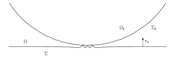
Figure 1. The hypersurfaces $\Sigma_{k}=\partial\Omega_{k}$ converge locally uniformly to $\Sigma=\partial\Omega$. Both the inward-pointing normal of $\Sigma$ and the re-scaled barycenters of $\Omega_{k}$ asymptote to the vector $e_{n}$.

The goal of this section is to show that $\Sigma$ is stable with respect to asymptotically constant variations, i.e., that

$$\int_{\Sigma}(|h|^{2}+Ric(\nu,\nu))\,(1+f)^{2}\,\mathrm{d}\mu\leq\int_{\Sigma}|\nabla f|^{2}\,\mathrm{d}\mu$$

for all $f\in C^{\infty}_{c}(\Sigma)$. To this end, we will study the second variation of area of $\Sigma_{k}=\partial\Omega_{k}$ with respect to a Euclidean translation; see Figure 1
Let $\chi\in C^{\infty}(M,TM)$ be a vector field with $\chi=e_{n}$ in $M\setminus B_{2}$ and $\chi=0$ in $B_{1}$. Let $u_{k},\,v_{k}\in C^{\infty}(\Sigma_{k})$ be the functions

$$u_{k}=g(\chi,\nu)\qquad\text{and}\qquad v_{k}=-h(\chi^{\top},\chi^{\top}).$$

We define the area radius of $\Sigma_{k}$ to be

$$\lambda(\Sigma_{k})=\left(\frac{|\Sigma_{k}|}{n\,\omega_{n}}\right)^{\frac{1}{n-1}}.$$

Recall from (47) that $\lambda(\Sigma_{k})\,H(\Sigma_{k})=(n-1)+o(1)$.

Lemma 23.

As $k\to\infty$,

$$\lambda(\Sigma_{k})^{1-n}\,\int_{\Sigma_{k}}u_{k}\,\mathrm{d}\mu=O(\lambda(\Sigma_{k})^{-\tau}).$$

Proof.

Since $\Sigma_{k}$ converges to $\Sigma$ locally smoothly, there are closed hypersurfaces $\hat{\Sigma}_{1},\,\hat{\Sigma}_{2},\ldots$ with

$$\circ\qquad B^{n}_{1}(0)\cap\hat{\Sigma}_{k}=\emptyset,\qquad\qquad\qquad\qquad\qquad\qquad\qquad\qquad\qquad$$

$$\circ\qquad\hat{\Sigma}_{k}\setminus B^{n}_{2}(0)=\Sigma_{k}\setminus B_{2},$$

$$\circ\qquad|B^{n}_{2}(0)\cap\hat{\Sigma}_{k}|_{\bar{g}}=O(1),\text{ and}$$

$$\circ\qquad h(\hat{\Sigma}_{k})=O(1).$$

Note that

$$\int_{\Sigma_{k}}g(\chi,\nu)\,\mathrm{d}\mu=\int_{\hat{\Sigma}_{k}}g(\chi,\nu)\,\mathrm{d}\mu-\int_{B_{2}\cap\hat{\Sigma}_{k}}g(\chi,\nu)\,\mathrm{d}\mu+\int_{B_{2}\cap\Sigma_{k}}g(\chi,\nu)\,\mathrm{d}\mu$$

Clearly,

$$\int_{B_{2}\cap\hat{\Sigma}_{k}}g(\chi,\nu)\,\mathrm{d}\mu=O(1).$$

By Lemma 46, $\limsup_{k\to\infty}|B_{2}\cap\Sigma_{k}|<\infty$, so that

$$\int_{B_{2}\cap\Sigma_{k}}g(\chi,\nu)\,\mathrm{d}\mu=O(1).$$

Using Lemma 64, we see that

$$\int_{\hat{\Sigma}_{k}}g(\chi,\nu)\,\mathrm{d}\mu=\int_{\hat{\Sigma}_{k}}\bar{g}(e_{n},\nu)\,\mathrm{d}\bar{\mu}+O(1)\,\int_{\hat{\Sigma}_{k}}|x|_{\bar{g}}^{-\tau}\,\mathrm{d}\bar{\mu}.$$

By the divergence theorem,

$$\int_{\hat{\Sigma}_{k}}\bar{g}(e_{n},\nu)\,\mathrm{d}\bar{\mu}=0.$$

Finally, by Lemma 46,

$$\int_{\hat{\Sigma}_{k}}|x|_{\bar{g}}^{-\tau}\,\mathrm{d}\bar{\mu}=O(\lambda(\Sigma_{k})^{n-1-\tau}).$$

The assertion follows from these estimates. ∎

Lemma 24.

There holds, as $k\to\infty$,

$$\lambda(\Sigma_{k})^{2-n}\,\int_{\Sigma_{k}}v_{k}+H\,u_{k}^{2}\,\mathrm{d}\mu=O(\lambda(\Sigma_{k})^{-\tau}).$$

Proof.

We continue with the notation introduced in the proof of Lemma 23. Using the area estimate from Lemma 46 and the curvature estimates (47) and (48), we see that

$$\int_{B_{2}\cap\Sigma_{k}}v_{k}+H\,u_{k}^{2}\,\mathrm{d}\mu=O(1).$$

Similarly,

$$\int_{B_{2}\cap\hat{\Sigma}_{k}}-h(\chi^{\top},\chi^{\top})+H\,g(\chi,\nu)^{2}\,\mathrm{d}\mu=O(1).$$

Using also Lemma 64, we obtain

$$v_{k}+H\,u_{k}^{2}=-\bar{h}(e_{n}^{\bar{\top}},e_{n}^{\bar{\top}})+\bar{H}\,\bar{g}(e_{n},\bar{\nu})^{2}+O(|x|_{\bar{g}}^{-1-\tau}).$$

Using Lemma 46, we get

$$\int_{\hat{\Sigma}_{k}}|x|_{\bar{g}}^{-1-\tau}\,\mathrm{d}\bar{\mu}=O(\lambda(\Sigma_{k})^{n-2-\tau}).$$

Combining these equations,

$$\int_{\Sigma_{k}}v_{k}+H\,u_{k}^{2}\,\mathrm{d}\mu=\int_{\hat{\Sigma}_{k}}-\bar{h}(e_{n}^{\bar{\top}},e_{n}^{\bar{\top}})+\bar{H}\,\bar{g}(e_{n},\bar{\nu})^{2}\,\mathrm{d}\bar{\mu}+O(\lambda(\Sigma_{k})^{n-2-\tau}).$$

Note that, by the first variation formula,

$$\int_{\hat{\Sigma}_{k}}-\bar{h}(e_{n}^{\bar{\top}},e_{n}^{\bar{\top}})+\bar{H}\,\bar{g}(e_{n},\bar{\nu})^{2}\,\mathrm{d}\bar{\mu}=0.$$

The assertion follows from these estimates. ∎

Fix $\eta\in C^{\infty}(\mathbb{R})$ with

• $\eta(t)=0$ if $t\leq 1$,

• $\eta(t)>0$ if $1<t<2$, and

• $\eta(t)=0$ if $t\geq 2$.

We define

$$\kappa_{k}=\lambda(\Sigma_{k})^{1-n}\,\int_{\Sigma_{k}}\eta\left(\lambda(\Sigma_{k})^{-1}\,|x|_{\bar{g}}\right)\,\mathrm{d}\mu\qquad\text{and}\qquad\kappa=\int_{S^{n-1}_{1}(e_{n})}\eta(|x|_{\bar{g}})\,\mathrm{d}\bar{\mu}.$$

Note that $\kappa>0$.

Lemma 25.

Passing to a subsequence, there holds $\kappa_{k}\to\kappa.$

Proof.

This follows from Proposition 58. ∎

Let $f\in C_{c}^{\infty}(M)$ be a function whose support is disjoint from the boundary of $M$. We define

$$\tilde{u}_{k}(x)=\begin{dcases}\alpha_{k}\,\lambda(\Sigma_{k})^{-\tau}\,\eta\left(\lambda(\Sigma_{k})^{-1}\,|x|_{\bar{g}}\right)\qquad&\text{if }x\notin B_{1},\\ 0&\text{else}.\end{dcases}$$

Here, $\alpha_{k}\in\mathbb{R}$ is chosen such that

(16) $$\int_{\Sigma_{k}}u_{k}+f+\tilde{u}_{k}\,\mathrm{d}\mu=0.$$

Using Lemma 23 and Lemma 25, we see that $\alpha_{k}=O(1)$. Next, we define

$$\tilde{v}_{k}(x)=\begin{dcases}\beta_{k}\,\lambda(\Sigma_{k})^{-1-\tau}\,\eta(\lambda(\Sigma_{k})^{-1}\,|x|_{\bar{g}})\qquad&\text{if }x\notin B_{1},\\ 0&\text{else},\end{dcases}$$

where $\beta_{k}\in\mathbb{R}$ is chosen such that

(17) $$\int_{\Sigma_{k}}v_{k}+\tilde{v}_{k}+H\,(u_{k}+f+\tilde{u}_{k})^{2}\,\mathrm{d}\mu=0.$$

Using Lemma 24, Lemma 25, and (47), we see that $\beta_{k}=O(1)$.
Note that there is $\varepsilon>0$ such that, for all $s\in(-\varepsilon,\varepsilon)$,

$$\Sigma_{k}(s)=\{\exp_{x}\left(U_{k}(x,s)\,\nu(\Sigma_{k})(x)\right):x\in\Sigma_{k}\}$$

where

$$U_{k}(x,s)=s\,(u_{k}+f+\tilde{u}_{k})(x)+\tfrac{1}{2}\,s^{2}\,(v_{k}+\tilde{v}_{k})(x)$$

is an embedded hypersurface in $M$ that bounds a region $\Omega_{k}(s)$.

Lemma 26.

There holds

$$\frac{d}{ds}\bigg{|}_{s=0}|\Omega_{k}(s)|=\frac{d^{2}}{ds^{2}}\bigg{|}_{s=0}|\Omega_{k}(s)|=0.$$

Proof.

This follows from Lemma 62 using (16) and (17). ∎

By Proposition 9, $\partial B_{r}$ intersects $\Sigma$ transversally for all $r>1$ sufficiently large. Increasing $r>1$ if necessary, we may arrange that

(18) $$\operatorname{spt}(f)\subset B_{r}.$$

For Proposition 27 below, let $u\in C^{\infty}(\Sigma)$ be the function given by $u=g(\chi,\nu)$.

Proposition 27.

There holds

$$\int_{B_{r}\cap\Sigma}(|h|^{2}+{Ric}(\nu,\nu))\,(u+f)^{2}\,\mathrm{d}\mu\leq\int_{B_{r}\cap\Sigma}|\nabla(u+f)|^{2}\,\mathrm{d}\mu+O(r^{n-3-\tau}).$$

Proof.

By Lemma 26, the variation $\{\Sigma_{k}(s)\}_{|s|<\varepsilon}$ is volume-preserving up to second order. Since $\Omega_{k}$ is isoperimetric, it follows that

$$\frac{d^{2}}{ds^{2}}\bigg{|}_{s=0}|\Sigma_{k}(s)|_{g}\geq 0.$$

By Lemma 62,

$$\frac{d^{2}}{ds^{2}}\bigg{|}_{s=0}|\Sigma_{k}(s)|_{g}=\int_{\Sigma_{k}}H\,\ddot{U}_{k}+H^{2}\,\dot{U}^{2}_{k}+|\nabla\dot{U}_{k}|^{2}-(|h|^{2}+{Ric}(\nu,\nu))\,\dot{{U}}^{2}_{k}\,\mathrm{d}\mu.$$

Note that $\tilde{v}_{k}(x)=\tilde{u}_{k}(x)=0$ if $|x|_{\bar{g}}\leq\lambda(\Sigma_{k})$. Using also the curvature estimates (47) and (48), that is, $|x|_{\bar{g}}\,h=O(1)$, we check that

• $H\,\tilde{v}_{k}=O(\lambda(\Sigma_{k})^{-2-\tau}),$

• $H^{2}\,\tilde{u}_{k}\,(u_{k}+f+\tilde{u}_{k})=O(\lambda(\Sigma_{k})^{-2-\tau})$,

• $g(\nabla\tilde{u}_{k},\nabla(u_{k}+f+\tilde{u}_{k}))=O(\lambda(\Sigma_{k})^{-2-\tau})$, and

• $(|h|^{2}+Ric(\nu,\nu))\,\tilde{u}_{k}\,(u_{k}+f+\tilde{u}_{k})=O(\lambda(\Sigma_{k})^{-2-\tau})$.

It follows that

$$\frac{d^{2}}{ds^{2}}\bigg{|}_{s=0}|\Sigma_{k}(s)|_{g} =\int_{\Sigma_{k}}H\,v_{k}+H^{2}\,(u_{k}+f)^{2}+|\nabla(u_{k}+f)|^{2}-(|h|^{2}+{Ric}(\nu,\nu))\,(u_{k}+f)^{2}\,\mathrm{d}\mu$$

$$\qquad+O(\lambda(\Sigma_{k})^{n-3-\tau}).$$

Note that $f=0$ on $\Sigma_{k}\setminus B_{r}$. Using Lemma 46, we have

$$\int_{\Sigma_{k}\setminus B_{r}}{Ric}(\nu,\nu)\,u_{k}^{2}\,\mathrm{d}\mu=O(1)\,\int_{\Sigma_{k}\setminus B_{r}}|x|_{\bar{g}}^{-2-\tau}\,\mathrm{d}\bar{\mu}=O(\lambda(\Sigma_{k})^{n-3-\tau})+O(r^{n-3-\tau}).$$

Similarly, using also Lemma 64, the curvature estimates (47) and (48), and (18), we check that

$$\int_{\Sigma_{k}\setminus B_{r}}H\,v_{k}+H^{2}\,u_{k}^{2}+|\nabla u_{k}|^{2}-|h|^{2}\,u_{k}^{2}\,\mathrm{d}\mu$$

$$\qquad=\int_{\Sigma_{k}\setminus B_{r}}\bar{H}\,\bar{v}_{k}+\bar{H}^{2}\,\bar{u}_{k}^{2}+|\bar{\nabla}\bar{u}_{k}|_{\bar{g}}^{2}-|\bar{h}|^{2}_{\bar{g}}\,\bar{u}_{k}^{2}\,\mathrm{d}\bar{\mu}+O(\lambda(\Sigma_{k})^{n-3-\tau})+O(r^{n-3-\tau})$$

where $\bar{u}_{k},\,\bar{v}_{k}\in C^{\infty}(\Sigma_{k})$ are given by $\bar{u}_{k}=\bar{g}(e_{n},\bar{\nu})$ and $\bar{v}_{k}=-\bar{h}(e_{n}^{\bar{\top}},e_{n}^{\bar{\top}}).$ For instance,

$$H\,v_{k}=\bar{H}\,\bar{v}_{k}+O(|x|_{\bar{g}}^{-2-\tau})$$

and

$$\int_{\Sigma_{k}\setminus B_{r}}|x|_{\bar{g}}^{-2-\tau}\,\mathrm{d}\bar{\mu}=O(\lambda(\Sigma_{k})^{n-3-\tau})+O(r^{n-3-\tau}).$$

Since $\Sigma_{k}\to\Sigma$ locally smoothly, we obtain, using also the integration by parts formula from Lemma 63,

$$\int_{\Sigma_{k}\setminus B_{r}}\bar{H}\,\bar{v}_{k}+\bar{H}^{2}\,\bar{u}_{k}^{2}+|\bar{\nabla}\bar{u}_{k}|_{\bar{g}}^{2}-|\bar{h}|^{2}_{\bar{g}}\,\bar{u}_{k}^{2}\,\mathrm{d}\bar{\mu}=O(1)\,\int_{\partial B_{r}\cap\Sigma}|\bar{h}(\Sigma)|_{\bar{g}}\,|e_{n}^{\bar{\top}}|_{\bar{g}}\,\mathrm{d}\bar{\ell}.$$

By Proposition 9, $|\bar{h}(\Sigma)|_{\bar{g}}=O(|y|_{\bar{g}}^{-1-\tau/2})$, $e_{n}^{\bar{\top}}=O(|y|_{\bar{g}}^{-\tau/2})$, and $|\partial B_{r}\cap\Sigma|_{\bar{g}}=O(r^{n-2})$. Thus,

$$\int_{\partial B_{r}\cap\Sigma}|\bar{h}(\Sigma)|_{\bar{g}}\,|e_{n}^{\bar{\top}}|_{\bar{g}}\,\mathrm{d}\bar{\ell}=O(r^{n-3-\tau}).$$

The assertion follows from the above estimates using (15), (47), and that $\Sigma_{k}\to\Sigma$ locally smoothly. ∎

Proposition 28.

Let $f\in C^{\infty}_{c}(\Sigma)$. There holds

$$\int_{\Sigma}(|h|^{2}+{Ric}(\nu,\nu))\,(1+f)^{2}\,\mathrm{d}\mu\leq\int_{\Sigma}|\nabla f|^{2}\,\mathrm{d}\mu.$$

Proof.

We may assume that the support of $f$ is disjoint from the boundary of $M$, which is stable. Letting $r\to\infty$ in Proposition 27 and using Corollary 21 and the dominated convergence theorem, we conclude that

(19) $$\int_{\Sigma}(|h|^{2}+{Ric}(\nu,\nu))\,(u+f)^{2}\,\mathrm{d}\mu\leq\int_{\Sigma}|\nabla(u+f)|^{2}\,\mathrm{d}\mu$$

for all $f\in C^{\infty}_{c}(\Sigma)$. Fix a function $\psi\in C^{\infty}_{c}(\mathbb{R})$ with $\psi(t)=1$ if $t\leq 1$. Let $\{f_{k}\}_{k=1}^{\infty}$ be the sequence of functions $f_{k}\in C_{c}^{\infty}(\Sigma)$ given by

$$f_{k}(x)=\begin{dcases}1-u(x)+f(x)\qquad&\text{if }x\in B_{1},\\ \psi(k^{-1}\,|x|_{\bar{g}})\,(1-u(x))+f(x)&\text{else}.\end{dcases}.$$

Note that, on $\Sigma\setminus B_{1}$,

(20) $$|\nabla f_{k}|^{2}\leq O(1)\,\big{(}|x|_{\bar{g}}^{-2}\,|u-1|^{2}+|\nabla u|^{2}+|\nabla f|^{2}\big{)}.$$

By Proposition 9,

$$|u-1|+|x|_{\bar{g}}\,|\nabla u|=O(|x|_{\bar{g}}^{-\tau/2}).$$

It follows that the right-hand side of (20) is integrable. The assertion now follows from applying (19) with $f_{k}$ in place of $f$, letting $k\to\infty$, and using the dominated convergence theorem. ∎

Remark 29.

Proposition 28 holds for all $f\in H^{1}_{\ell oc}(\Sigma)$ for which there are $f_{1},\,f_{2},\ldots\in C^{\infty}_{c}(\Sigma)$ with $\nabla f_{k}\to\nabla f\text{ in }L^{2}(\Sigma)$, as can be seen using the Sobolev inequality.

The following Proposition is a consequence of Proposition 28 using arguments of R. Schoen and S.-T. Yau [pmt] and of A. Carlotto [Carlottocalcvar].

Proposition 30.

Suppose that $R\geq 0$ along the non-compact component of $\Sigma$. Then the non-compact component of $\Sigma$ is totally geodesic and isometric to flat $\mathbb{R}^{n-1}$. Moreover, there holds $R={Ric}(\nu,\nu)=0$ along the non-compact component of $\Sigma$.

Proof.

Let $\Sigma^{0}$ be the non-compact component of $\Sigma$. Arguing as in the proof of [Carlottocalcvar, Theorem 2] using Lemma 22 and the stability with respect to asymptotically constant variations asserted in Proposition 28, we see that the scalar curvature of $(\Sigma^{0},g|_{\Sigma^{0}})$ vanishes. By the rigidity statement of the positive mass theorem [schoenconformal, Lemma 3 and Proposition 2], $(\Sigma^{0},g|_{\Sigma^{0}})$ is isometric to flat $\mathbb{R}^{n-1}$.
As explained in [montecatini, p. 35], Proposition 28 implies that

$$\int_{\Sigma^{0}}|h|^{2}+{Ric}(\nu,\nu)\,\mathrm{d}\mu\leq 0.$$

Using the Gauss equation and that $\Sigma^{0}$ is scalar flat, we have

$$|h|^{2}+{Ric}(\nu,\nu)=\frac{1}{2}\,(|h|^{2}+R).$$

In conjunction with $R\geq 0$, we obtain that $h=0$ and that $R={Ric}(\nu,\nu)=0$ along $\Sigma^{0}$. ∎

4. Proof of Theorem 2

In this section, $(M,g)$ is a Riemannian manifold of dimension $3<n\leq 7$ that is asymptotically flat of rate $\tau>n-3$ and which has non-negative scalar curvature and positive mass.
We defer the proof of the following lemma to the end of this section.

Lemma 31.

Let $p_{1},\,p_{2}$ be points in the interior of $M$. There exists $U$ open and compactly contained in the interior of $M$ with $p_{1},\,p_{2}\in U$ such that the following holds. For all $r>0$ sufficiently small, there exist $W\subset U$ open with $p_{1},\,p_{2}\in W$ and a family $\{g_{t}\}_{t\in(0,1)}$ of Riemannian metrics $g_{t}$ on $M$ such that

(21) $$\circ\qquad g_{t}\to g\text{ smoothly as }t\to 0,$$

(22) $$\circ\qquad g_{t}=g\text{ in }M\setminus W,$$

(23) $$\circ\qquad g_{t}<g\text{ in }W,\text{ and}$$

(24) $$\circ\qquad R(g_{t})>0\text{ in }\{x\in W:\operatorname{dist}_{g}(x,p_{2})>r\}.$$

Let $\Omega_{1},\,\Omega_{2},\ldots\subset M$ be isoperimetric regions with $|\Omega_{k}|\to\infty$ and such that $\Omega_{k}$ converges locally smoothly to a region $\Omega\subset M$ whose boundary $\Sigma=\partial\Omega$ is non-compact and area-minimizing.

Proposition 32.

Let $p$ be a point in the interior of $M$. There exist $U$ open and compactly contained in the interior of $M$, Riemannian metrics $\tilde{g}_{1},\,\tilde{g}_{2},\ldots$ on $M$, and regions $\,\tilde{\Omega}_{1},\,\tilde{\Omega}_{2},\ldots$, and $\Omega_{p}\subset M$ with the following properties.

• $\operatorname{spt}(\tilde{g}_{k}-g)\subset U$ for all $k$ and $\tilde{g}_{k}\to g$ smoothly.

• $\tilde{\Omega}_{k}$ is an isoperimetric region in $(M,\tilde{g}_{k}$) and $|\tilde{\Omega}_{k}|_{\tilde{g}_{k}}\to\infty$.

• $\tilde{\Omega}_{k}\to\Omega_{p}$ locally smoothly.

• $\partial\Omega_{p}$ is a non-compact area-minimizing boundary in $(M,g)$ that is stable with respect to asymptotically constant variations and $p\in\partial\Omega_{p}$.

Proof.

We first assume that the boundary of $M$ is empty.
We choose $p_{1}\in\Sigma$ and let $p_{2}=p$. Let $U\subset M$ be the open set from Lemma 31 and $r>0$ be small enough so that the conclusion of Lemma 31 holds. According to Lemma 31, there is $W\subset U$ open and a family $\{g_{t}\}_{t\in(0,1)}$ of Riemannian metrics $g_{t}$ on $M$ satisfying (21), (22), (23), and (24).
Let $t\in(0,1)$. Recall the isoperimetric profile $A_{g}$ defined in (49). Let $c(t)=|W|_{g}-|W|_{g_{t}}$. Note that

• $c(t)>0$ by (23) and

• $c(t)=o(1)$ as $t\to 0$ by (21).

Since $\partial\Omega_{k}\to\Sigma$ locally smoothly and $\Sigma\cap W\neq\emptyset$, it follows from $\eqref{g properties 5}$ that there is $\varepsilon(t)>0$ such that, for all $k$ sufficiently large,

(25) $$|\partial\Omega_{k}|_{g_{t}}+\varepsilon(t)<|\partial\Omega_{k}|_{g}.$$

Using Lemma 60, we see that

(26) $$|\partial\Omega_{k}|_{g}=A_{g}(|\Omega_{k}|_{g})\leq A_{g}(V)+o(1)$$

for any amount of volume $V$ such that $|\Omega_{k}|_{g}-c(t)\leq V\leq|\Omega_{k}|_{g}+c(t)$. By Lemma 61, for every $k$ sufficiently large, there exists an isoperimetric region $\Omega_{k}(t)\subset M$ with respect to $g_{t}$ such that $|\Omega_{k}(t)|_{g_{t}}=|\Omega_{k}|_{g_{t}}$.
We claim that there is $\tilde{W}\Subset W$ open such that, for all $k$ sufficiently large,

(27) $$\tilde{W}\cap\partial\Omega_{k}(t)\neq\emptyset.$$

To see this, assume the contrary. Passing to a subsequence and using (22) and Lemma 46, we see that

(28) $$|\partial\Omega_{k}(t)|_{g_{t}}=|\partial\Omega_{k}(t)|_{g}+o(1).$$

Using (23), we have

$$|\Omega_{k}(t)|_{g}\leq|\Omega_{k}(t)|_{g_{t}}+c(t)=|\Omega_{k}|_{g_{t}}+c(t)\leq|\Omega_{k}|_{g}+c(t).$$

Similarly, $|\Omega_{k}(t)|_{g}\geq|\Omega_{k}|_{g}-c(t).$ Using (26) with $V=|\Omega_{k}(t)|_{g}$, we conclude that

$$|\partial\Omega_{k}(t)|_{g}\geq|\partial\Omega_{k}|_{g}-o(1).$$

This is not compatible with (25) and (28).
By Proposition 58, $\Omega_{k}(t)$ converges locally smoothly to a region $\Omega(t)$ with non-compact boundary $\Sigma(t)$ that is area-minimizing with respect to $g_{t}$. Using (27), we see that $\Sigma(t)$ intersects the closure of $\tilde{W}$. Using Proposition 30 and (24), it follows that, in fact, $\{x\in M:\operatorname{dist}(x,p)<r\}\cap\Sigma(t)\neq\emptyset$.
Passing to a subsequence, we see that, as $t\to 0$, $\Omega(t)$ converges locally smoothly to a a region $\Omega_{p}(r)\subset M$ with non-compact boundary $\Sigma_{p}(r)$ that is area-minimizing with respect to $g$ such that $\{x\in M:\operatorname{dist}(x,p)\leq r\}\cap\Sigma_{p}(r)\neq\emptyset$. Moreover, passing to a subsequence, we see that, as $r\to 0$, $\Omega_{p}(r)$ converges locally smoothly to a region $\Omega_{p}$ with non-compact boundary $\Sigma_{p}$ that is area-minimizing with respect to $g$ and such that $p\in\Sigma_{p}$.
By a diagonal argument, we see that there are Riemannian metric $\tilde{g}_{1},\,\tilde{g}_{2},\ldots$ on $M$ and regions $\,\tilde{\Omega}_{1},\,\tilde{\Omega}_{2},\ldots\subset M$ with the asserted properties. Repeating the argument that led to Proposition 28, we see that $\Sigma_{p}$ is stable with respect to asymptotically constant variations in the sense of Proposition 28. This completes the proof in the case where the boundary of $M$ is empty.
In the case where the boundary of $M$ is an outermost minimal surface, we note that the boundary of $M$ is also an outermost minimal surface with respect to $g_{t}$ for all sufficiently small $t>0$. The rest of the proof only requires formal modifications. ∎

Proof of Theorem 2.

Let $(M,g)$ be asymptotically flat of rate $\tau>n-3$ with non-negative scalar curvature. Suppose that there are isoperimetric regions $\Omega_{1},\,\Omega_{2},\ldots$ in $(M,g)$ with $|\Omega_{k}|\to\infty$ such that $\Omega_{k}$ converges locally smoothly to a region $\Omega\subset M$ whose boundary $\Sigma=\partial\Omega$ is non-compact and area-minimizing.
Suppose for a contradiction, that $(M,g)$ has positive mass $m$.
We first assume that the boundary of $M$ is empty.
Our goal is to show that the curvature tensor ${Rm}$ vanishes everywhere.
Let $p\in M$. We first assume that $p\in\Sigma$. Using Proposition 32, Proposition 30, and standard convergence results from geometric measure theory, we see that there are mutually distinct connected non-compact area-minimizing boundaries $\Sigma_{1},\,\Sigma_{2},\ldots\subset M$ such that

• $\Sigma_{k}$ is isometric to flat $\mathbb{R}^{n-1}$ for all $k$,

• $\Sigma_{k}$ is totally geodesic for all $k$, and

• $\Sigma_{k}\to\Sigma$ locally smoothly.

Let $W,\,X,\,Y,\,Z$ be tangent fields along $\Sigma$. Note that

(29) $${Rm}(W,\,X,\,Y,\,Z)=0.$$

Indeed, this follows from the Gauss equation, using that $\Sigma$ is isometric to flat $\mathbb{R}^{n-1}$ and totally geodesic. Similarly, using the Codazzi equation, we obtain

(30) $${Rm}(W,\,X,\,Y,\nu)=0.$$

By the Hopf maximum principle, $\Sigma$ and $\Sigma_{k}$ are either disjoint or intersect transversally. In the latter case, ${Rm}=0$ along the intersection. We may therefore assume that there is a neighborhood $U$ of $p$ such that $U\cap\Sigma\cap\Sigma_{k}=\emptyset$ for all $k\geq 1$.
Since $\Sigma$ and $\Sigma_{k}$ are totally geodesic, the components of $\Sigma\cap\Sigma_{k}$ are totally geodesic and therefore hyperplanes of $\Sigma$. Since $\Sigma$ and $\Sigma_{k}$ are embedded, the components of $\Sigma\cap\Sigma_{k}$ must be parallel. It follows that, passing to a subsequence, there are three cases.

• For every $k$, $\Sigma\cap\Sigma_{k}=\emptyset$.

• For every $k$, $\Sigma\cap\Sigma_{k}$ consists of a single hyperplane in $\Sigma$.

• For every $k$, $\Sigma\cap\Sigma_{k}$ consists of at least two parallel hyperplanes in $\Sigma$.

In the second and the third case, let $\Sigma^{0}_{k}$ be the closure of the component of $\Sigma\setminus\Sigma_{k}$ that contains $p$. Note that $\Sigma^{0}_{k}$ is isometric to a half-space in the second case and isometric to a slab in the third case. Since $U\cap\Sigma\cap\Sigma_{k}=\emptyset$, it follows that $\liminf_{k\to\infty}\operatorname{dist}(p,\partial\Sigma^{0}_{k})>0.$
In the first case, we may argue exactly as in [CCE, p. 993]. Specifically, we may represent $\Sigma_{k}$ as the graph of a positive function $u_{k}$ over larger and larger domains, exhausting $\Sigma$ as $k\to\infty$. By the Harnack inequality [gilbargtrudinger, §8.8], $u_{k}$ is bounded by a multiple of $u_{k}(p)$ locally in $\Sigma$ as $k\to\infty$. Using the first variation of the second fundamental form and proceeding as in [simonstrict, p. 333], we obtain a positive function $f\in C^{\infty}(\Sigma)$ such that

(31) $$\nabla_{X,Y}^{2}f+{Rm}(X,\nu,\nu,Y)\,f=0$$

for all tangent fields $X,\,Y$ of $\Sigma$. Tracing (31) and using that ${Ric}(\nu,\nu)=0$ along $\Sigma$, we see that $f$ is harmonic. By the Liouville theorem, $f$ is equal to a constant. It follows that ${Rm}(X,\nu,\nu,Y)=0$. In conjunction with (29) and (30), we conclude that ${Rm}=0$ along $\Sigma$ and in particular at $p$.
In the second case, if $\limsup_{k\to\infty}\operatorname{dist}(p,\partial\Sigma^{0}_{k})=\infty$, we may argue as in the first case. If $\operatorname{dist}(p,\partial\Sigma^{0}_{k})=O(1)$, then, passing to a subsequence, we may assume that $\Sigma_{k}^{0}$ converges locally smoothly to a half-space $\Sigma^{0}\subset\Sigma$. As before, we may represent $\Sigma^{0}_{k}$ as the graph of a smooth function $u_{k}$ over larger and larger domains, exhausting $\Sigma^{0}$ as $k\to\infty$. Arguing as in the first case, using also the Boundary Harnack inequality (see, e.g., [caffarelli, Theorem 11.5]), we obtain a harmonic function $f\in C^{\infty}(\Sigma^{0})$ that satisfies (31) in $\Sigma^{0}$, $f=0$ on $\partial\Sigma^{0}$, and $f>0$ away from $\partial\Sigma^{0}$. By [shortproofs, Theorem I], $f$ is a linear function. As before, it follows that ${Rm}=0$ along $\Sigma$ and in particular at $p$.
Finally, suppose for a contradiction that the third case arises. We may assume that, passing to a subsequence, $\Sigma_{k}^{0}$ converges locally to a slab $\Sigma^{0}\subset\Sigma$. As in the previous case, we obtain a harmonic function $f\in C^{\infty}(\Sigma^{0})$ that satisfies (31) in $\Sigma^{0}$, $f=0$ on $\partial\Sigma^{0}$, and $f>0$ away from $\partial\Sigma^{0}$. Using (31), we see that $|\nabla f|$ is bounded from above by a positive constant on $\partial\Sigma^{0}$. This is not compatible with Lemma 66.
Now, let $p\in M\setminus\Sigma$. By Proposition 32, there exists a non-compact area-minimizing boundary $\Sigma_{p}$ with $p\in\Sigma_{p}$ that is stable with respect to asymptotically constant variations. Repeating the argument above with $\Sigma_{p}$ in place of $\Sigma$, we see that $Rm=0$ along $\Sigma_{p}$. Since $(M,g)$ is asymptotically flat, it follows that $(M,g)$ is isometric to flat $\mathbb{R}^{n}$. This is not compatible with $m>0$. This completes the proof in the case where the boundary of $M$ is empty.
The case where the boundary of $M$ is an outermost minimal surface only requires formal modifications. ∎

Proof of Corollary 4.

Let $(M,g)$ be asymptotically flat of rate $\tau>n-3$ with non-negative scalar curvature and positive mass $m$. Suppose, for a contradiction, that there are isoperimetric regions $\Omega_{1},\,\Omega_{2},\ldots$ in $(M,g)$ with $|\Omega_{k}|\to\infty$ and a compact set $K\subset M$ disjoint from the boundary of $M$ such that $K\cap\partial\Omega_{k}\neq\emptyset$ for all $k$.
By Proposition 58, $\Omega_{k}$ converges locally smoothly to a region $\Omega\subset M$ whose boundary $\Sigma=\partial\Omega$ is non-compact and area-minimizing. By Theorem 2, $(M,g)$ is isometric to flat $\mathbb{R}^{n}$. This is not compatible with $m>0$. ∎

Proof of Lemma 31.

Arguing as in [chaoli, p. 21], we see that there is $r_{0}>0$ depending only on $(M,g)$ with the following property. Given $0<r<r_{0}$ and $q\in M$, there exists a function $v_{r,q}\in C^{\infty}(M)$ satisfying

(32) $$\circ\qquad v_{r,q}=0\text{ in }\{x\in M:\operatorname{dist}_{g}(x,q)\geq 6\,r\},\qquad\qquad\qquad\qquad\qquad$$

(33) $$\circ\qquad v_{r,q}<0\text{ in }\{x\in M:\operatorname{dist}_{g}(x,q)<6\,r\},\text{ and}$$

(34) $$\circ\qquad\Delta v_{r,q}<0\text{ in }\{x\in M:r<\operatorname{dist}_{g}(x,q)<6\,r\}.$$

Decreasing $r>0$ if necessary, we may choose points $q_{1},\ldots,q_{N}\in M$ with $q_{1}=p_{1}$ and $q_{N}=p_{2}$ such that

(35) $$\{x\in M:\operatorname{dist}(x,q_{i})\leq r\}\subset\{x\in M:3\,r\leq\operatorname{dist}(x,q_{i+1})\leq 5\,r\}\text{ for all }i\leq N-1\text{ and}$$

$$\{x\in M:\operatorname{dist}(x,q_{i})\leq 6\,r\}\text{ is disjoint from the boundary of }M\text{ for all }1\leq i\leq N;$$

see Figure 2.

Figure 2. An illustration of the construction in Lemma 31. The open set $W$ is bounded by the solid black line. The function $v$ is super-harmonic outside of the hatched region.

Define $a_{1},\ldots,a_{N}$ recursively by $a_{1}=1$ and, for $i=2,\ldots,N$,

$$a_{i}=1+\frac{\sup\{\Delta v_{r,q_{i-1}}(x):\operatorname{dist}(x,q_{i-1})<r\}}{|\inf\{\Delta v_{r,q_{i}}(x):3\,r\leq\operatorname{dist}(x,q_{i})\leq 5\,r\}|}\,a_{i-1}.$$

Let

$$W=\bigcup_{i=1}^{N}\{x\in M:\operatorname{dist}(x,q_{i})<6\,r\}\qquad\text{and}\qquad v=\sum_{i=1}^{N}a_{i}\,v_{r,q_{i}}.$$

Note that

• $v=0$ in $M\setminus W$ by (32),

• $v<0$ in $W$ by (33), and

• $\Delta v<0$ in $\{x\in W:\operatorname{dist}(x,p_{2})\geq r\}$ by (34) and (35).

For all $\delta>0$ sufficiently small, the Riemannian metrics

$$g_{t}=(1+t\,\delta\,v)^{\frac{4}{n-2}}\,g$$

where $t\in(0,1)$ satisfy the properties asserted in the lemma.∎

5. Proof of Theorem 5

Let $3<n\leq 7$ and $(M,g)$ be spatial Schwarzschild with mass $m=2$, i.e.,

$$M=\{x\in\mathbb{R}^{n}:|x|_{\bar{g}}\geq 1\}\qquad\text{and}\qquad g=\phi^{\frac{4}{n-2}}\,\bar{g}$$

where $\phi\in C^{\infty}(M)$ is given by

$$\phi(x)=1+|x|_{\bar{g}}^{2-n}.$$

The goal of this section is to show that there are infinitely many mutually disjoint non-compact area-minimizing hypersurfaces in $(M,g)$.
Let $t,\,s>0$. For the next lemma, we choose the following orientations.

• $M\cap(\mathbb{R}^{n-1}\times\{t\})$ is oriented by the normal in direction of $-e_{n}$.

• $M\cap(S^{n-2}_{s}(0)\times\mathbb{R})$ is oriented by the normal pointing away from the vertical axis.

Lemma 33.

Let $t,\,s>0$. The following hold.

• $M\cap(\mathbb{R}^{n-1}\times\{t\})$ is strictly mean convex.

• $M\cap(S^{n-2}_{s}(0)\times\mathbb{R})$ is strictly mean convex.

• $S^{n-1}_{1}(0)$ is minimal.

Let $r>2,$ $z>0$, and $\Sigma_{r,z}$ be the least area hypersurface in $(M,g)$ with

$$\partial\Sigma_{r,z}=S^{n-2}_{r}(0)\times\{z\}.$$

By the convex hull property and Lemma 33, $\Sigma_{r,z}$ is a vertical graph with finite slope near $\partial\Sigma_{r,z}$.

Lemma 34.

$\Sigma_{r,z}$ is axially symmetric with respect to $e_{n}$.

Proof.

Let $\pi\subset\mathbb{R}^{n}$ be a hyperplane through the origin with $e_{n}\in\pi$. Let $\Pi:\mathbb{R}^{n}\to\mathbb{R}^{n}$ be the reflection through $\pi$, $\mathbb{R}^{n}_{\pm}$ be the components of $\mathbb{R}^{n}\setminus\pi$, and $\Sigma_{r,z}^{\pm}=\mathbb{R}^{n}_{\pm}\cap\Sigma_{r,z}$. Note that $M\cap\pi$ is minimal in $(M,g)$. By the Hopf maximum principle, it follows that $\Sigma_{r,z}$ and $\pi$ intersect transversally. In particular,

(36) $$|\Sigma_{r,z}^{+}|+|\Sigma_{r,z}^{-}|=|\Sigma_{r,z}|.$$

Moreover, $\tilde{\Sigma}_{r,z}=\Sigma_{r,z}^{+}\cup\Pi(\Sigma_{r,z}^{+})\cup(\Sigma_{r,z}\cap\pi)$ is a Lipschitz surface with $\partial\tilde{\Sigma}_{r,z}=\partial\Sigma_{r,z}$. Using that $g$ is rotationally symmetric, the area-minimizing property of $\Sigma_{r,z}$, and (36), we conclude that $2\,|\Sigma_{r,z}^{+}|=2\,|\Sigma_{r,z}^{-}|=|\Sigma_{r,z}|$. It follows that $|\tilde{\Sigma}_{r,z}|=|\Sigma_{r,z}|$. Using again that $\Sigma_{r,z}$ is area-minimizing, we see that $\tilde{\Sigma}_{r,z}$ intersects $\pi$ orthogonally. In particular, $\tilde{\Sigma}_{r,z}$ is smooth. By unique continuation [uniquecontinuation, p. 235], $\tilde{\Sigma}_{r,z}=\Sigma_{r,z}$. The assertion follows. ∎

Lemma 35.

$\Sigma_{r,z}\setminus\partial\Sigma_{r,z}$ is contained in the cylinder $B^{n-1}_{r}(0)\times(z,\infty).$

Proof.

This follows from Lemma 33 and the maximum principle. ∎

Lemma 36.

$\Sigma_{r,z}$ is a vertical graph over $\{y\in\mathbb{R}^{n-1}:|y|_{\bar{g}}\leq r\}$.

Proof.

Suppose, for a contradiction, that $\Sigma_{r,z}\setminus\partial\Sigma_{r,z}$ is not a graph over $B^{n-1}_{r}(0)$. Using Lemma 34 and Lemma 35, it follows that $\Sigma_{r,z}$ touches $S^{n-2}_{s}(0)\times\mathbb{R}$ from the inside for some $s\in(0,r)$. This is not compatible with Lemma 33 and the maximum principle. ∎

By Lemma 34 and Lemma 36, there is $f_{r,z}\in C^{\infty}(\mathbb{R})$ with $f_{r,z}(r)=z$ and $f^{\prime}_{r,z}(0)=0$ such that

$$\Sigma_{r,z}=\{\left(y,f_{r,z}(|y|_{\bar{g}})\right):y\in\mathbb{R}^{n-1}\text{ with }|y|_{\bar{g}}\leq r\}.$$

Lemma 37.

There holds, for all $t\in(0,r)$,

$$\bigg{(}t^{n-2}\frac{f^{\prime}_{r,z}(t)}{\sqrt{1+f^{\prime}_{r,z}(t)^{2}}}\bigg{)}^{\prime}=-\frac{2\,(n-1)}{1+(t^{2}+f_{r,z}(t)^{2})^{-\frac{n-2}{2}}}\,\frac{t^{n-2}}{(t^{2}+f_{r,z}(t)^{2})^{\frac{n}{2}}}\,\frac{f_{r,z}(t)-f_{r,z}^{\prime}(t)\,t}{\sqrt{1+f^{\prime}(t)^{2}}}.$$

Proof.

This follows from the conformal transformation formula of the mean curvature,

(37) $$\phi^{\frac{2}{n-2}}\,H=\bar{H}+\frac{2\,(n-1)}{n-2}\phi^{-1}\,\bar{D}_{\bar{\nu}}\phi,$$

using that $\Sigma_{r,z}$ is minimal. Here, $\bar{\nu}$ is the Euclidean unit normal of $\Sigma_{r,z}$ pointing in direction of $e_{n}$. ∎

Lemma 38.

There holds

$$0\leq\sup_{z>0}\limsup_{r\to\infty}\left[f_{r,z}(4\,(n-1))-z\right]<\infty.$$

Moreover, as $z\to 0$,

$$\limsup_{r\to\infty}f_{r,z}(z^{-2})=z+o(z).$$

Proof.

Using Lemma 33 and the maximum principle, we see that $f^{\prime}_{r,z}(t)\leq 0$ for all $t\in(0,r)$. Using Lemma 37 and the Cauchy-Schwarz inequality, we have, for all $t\in(0,r)$,

$$\bigg{(}t^{n-2}\,\frac{f_{r,z}^{\prime}(t)}{\sqrt{1+f_{r,z}^{\prime}(t)^{2}}}\bigg{)}^{\prime}\geq-2\,(n-1)\,\frac{t^{n-2}}{(t^{2}+f_{r,z}(t)^{2})^{\frac{n-1}{2}}}.$$

Integrating, we obtain

(38) $$\frac{f_{r,z}^{\prime}(t)}{\sqrt{1+f_{r,z}^{\prime}(t)^{2}}}\geq-2\,(n-1)\,t^{2-n}\,\int_{0}^{t}\frac{s^{n-2}}{(s^{2}+f_{r,z}(s)^{2})^{\frac{n-1}{2}}}\,\mathrm{d}s.$$

Note that $s^{2}+f_{r,z}(s)^{2}\geq 1$. Consequently, for all $t\geq 1$,

(39) $$\int_{0}^{t}\frac{s^{n-2}}{(s^{2}+f_{r,z}(s)^{2})^{\frac{n-1}{2}}}\,\mathrm{d}s\leq\int_{0}^{1}\,\mathrm{d}s+\int_{1}^{t}\,s^{-1}\,\mathrm{d}s=1+\log(t).$$

It follows that

$$2\,(n-1)\,t^{2-n}\,\int_{0}^{t}\frac{s^{n-2}}{(s^{2}+f_{r,z}(s)^{2})^{\frac{n-1}{2}}}\,\mathrm{d}s\leq\frac{1}{2}$$

provided that $t\geq 4\,(n-1)$. Note that

$$\frac{1}{2}\,f^{\prime}_{r,z}(t)\geq\frac{f^{\prime}_{r,z}(t)}{\sqrt{1+f^{\prime}_{r,z}(t)^{2}}}\qquad\text{provided that}\qquad\frac{f^{\prime}_{r,z}(t)}{\sqrt{1+f^{\prime}_{r,z}(t)^{2}}}\geq-\frac{1}{2}.$$

In conjunction with (38) and (39), we obtain

$$f_{r,z}^{\prime}(t)\geq-4\,(n-1)\,t^{2-n}\,(\log(t)+1)$$

provided that $t\geq 4\,(n-1)$. Since $f_{r,z}(r)=z$, we conclude that

$$z\leq f_{r,z}(4\,(n-1)) \leq z+4\,(n-1)\,\int^{r}_{4\,(n-1)}t^{2-n}\,(\log(t)+1)\,\mathrm{d}t$$

for all $r\geq 4\,(n-1)$. Note that, since $n\geq 4$,

$$\int^{r}_{4\,(n-1)}t^{2-n}\,(\log(t)+1)\,\mathrm{d}t\leq\int^{\infty}_{4\,(n-1)}t^{2-n}\,(\log(t)+1)\,\mathrm{d}t<\infty.$$

Likewise, we obtain, as $z\to 0$,

$$\limsup_{r\to\infty}f_{r,z}(z^{-2})\leq z+4\,(n-1)\,\int^{\infty}_{z^{-2}}t^{2-n}\,(\log(t)+1)\,\mathrm{d}t=z+o(z).$$

The assertion follows. ∎

Lemma 39.

Let $z>0$. There exists a sequence $\{r_{k}\}_{k=1}^{\infty}$ with $r_{k}\to\infty$ such that $\Sigma_{z,r_{k}}$ converges locally smoothly to a non-compact area-minimizing hypersurface $\Sigma_{z}\subset M$ that is axially symmetric with respect to $e_{n}$ and satisfies

(40) $$\inf\{x^{n}:x\in\Sigma_{z}\}=z.$$

Proof.

This follows from Lemma 35, Lemma 38, and standard compactness results from geometric measure theory. ∎

Proposition 40.

The following hold.

• As $z\to 0$, $\Sigma_{z}$ converges locally smoothly to a non-compact area-minimizing hypersurface $\Sigma_{0}\subset M$ with $\inf\{x^{n}:x\in\Sigma_{0}\}=0$.

• As $z\to\infty$, $-z+\Sigma_{z}$ converges locally smoothly to a Euclidean plane.

• The family $\{\Sigma_{z}\}_{z>0}$ forms a smooth foliation of the component of $M\setminus\Sigma_{0}$ that lies above $\Sigma_{0}$.

• $\Sigma_{z}$ is not stable with respect to asymptotically constant perturbations for any $z\geq 0$.

Proof.

Let $z_{1},\,z_{2}>0$ with $z_{1}\neq z_{2}$. Since $\Sigma_{z_{1}}$ and $\Sigma_{z_{2}}$ are area-minimizing and axially symmetric with respect to $e_{n}$, $\Sigma_{z_{1}}$ and $\Sigma_{z_{2}}$ are disjoint. Using also (40), we see that, as $z\to 0$, $\Sigma_{z}$ converges locally smoothly to a non-compact area-minimizing hypersurface $\Sigma_{0}\subset M$ with $\inf\{x^{n}:x\in\Sigma_{0}\}=0$. Moreover, using Lemma 38, we see that, as $z\to\infty$, $-z+\Sigma_{z}$ converges locally smoothly to a non-compact hypersurface $\Sigma$ that is area-minimizing with respect to $\bar{g}$. By Lemma 48, $\Sigma$ is a Euclidean plane.
Let $z>0$. By (37), $t+\Sigma_{z}$ is strictly mean-convex for every $t>0$ when oriented by the unit normal in direction of $e_{n}$. In conjunction with (40) and the maximum principle, it follows that $\Sigma_{z^{\prime}}\to\Sigma_{z}$ locally smoothly as $z^{\prime}\searrow z$. Let $\{z_{i}\}_{i=1}^{\infty}$ be a sequence of numbers $0<z_{i}<z$ with $z_{i}\to z$. Passing to a subsequence and using (40), we see that $\Sigma_{z_{i}}$ converges locally smoothly to a non-compact area-minimizing hypersurface $\Sigma^{\prime}_{z}$ that lies below $\Sigma_{z}$, is axially symmetric with respect to $e_{n}$, and satisfies $\inf\{x^{n}:x\in\Sigma^{\prime}_{z}\}=z$. Since both $\Sigma_{r,z}$, $r\geq 2$, and $\Sigma^{\prime}_{z}$ are area-minimizing and axially symmetric with respect to $e_{n}$, $\Sigma_{r,z}$ lies below $\Sigma^{\prime}_{z}$ for every $r\geq 2$. It follows that $\Sigma^{\prime}_{z}=\Sigma_{z}$. Consequently, $\{\Sigma_{z}\}_{z>0}$ forms a smooth foliation; see Figure 3.
Finally, suppose for a contradiction, that $\Sigma_{z}$ is stable with respect to asymptotically constant perturbations for some $z\geq 0$. By Proposition 30, $\Sigma_{z}$ is totally geodesic. It follows that $\Sigma_{z}=S^{n}_{1}(0)$. This is not compatible with $\Sigma_{z}$ being non-compact.
The assertion follows. ∎

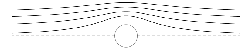
Figure 3. An illustration of the foliation $\{\Sigma_{z}\}_{z\geq 0}$ whose leaves are depicted by the solid black lines. The horizon is depicted by the gray line. $\Sigma_{0}$ asymptotes to the plane $\{x^{n}=0:x\in M\}$ depicted by the dashed black line.

6. Proof of Theorem 6

Let $3<n\leq 7$ and $(n-2)/2<\tau<n-2$. In this section, we use the gluing technique developed by A. Carlotto and R. Schoen [SchoenCarlotto] to construct a Riemannian manifold of dimension $n$ which is asymptotically flat of rate $\tau$ with non-negative scalar curvature and positive mass and which admits a non-compact area-minimizing boundary that is stable with respect to asymptotically constant variations (1).

Lemma 41.

There exists a Riemannian metric $g$ on $\mathbb{R}^{n}$ which is asymptotically flat of rate $\tau$ with non-negative scalar curvature and positive mass such that

$$g=\bar{g}\text{ on }\{x\in\mathbb{R}^{n}:x^{n}\leq 2+|x-x^{n}\,e_{n}|_{\bar{g}}\}.$$

Proof.

The Riemannian metric

$$\hat{g}=\left[1+(1+|x|_{\bar{g}}^{2\,n-4})^{-\frac{1}{2}}\right]^{\frac{4}{n-2}}\,\bar{g}$$

is asymptotically flat of rate $n-2$ with non-negative scalar and mass $2$. The assertion follows from localizing $(\mathbb{R}^{n},\hat{g})$ to the cone $\{x\in\mathbb{R}^{n}:x^{n}>2+|x-x^{n}\,e_{n}|_{\bar{g}}\}$ using [SchoenCarlotto, Theorem 2.3]. ∎

Lemma 42.

Let $(n-2)/2<\tilde{\tau}<\tau$ and $g$ be as in Lemma 41. There exists a conformally flat Riemannian metric $\tilde{g}$ on $\mathbb{R}^{n}$ that is asymptotically flat of rate $\tilde{\tau}$ with the following properties:

• $\tilde{g}\leq g$.

• $\tilde{g}<g$ on $\{x\in\mathbb{R}^{n}:x^{n}\geq 2+|x-x^{n}\,e_{n}|_{\bar{g}}\}$.

• $\tilde{g}=\bar{g}$ on $\{x\in\mathbb{R}^{n}:x^{n}\leq 0\}$.

• $\tilde{g}$ is axially symmetric with respect to $e_{n}$.

• There holds, for all $x\in\mathbb{R}^{n}$,

  $$\sum_{i=1}^{n-1}x^{i}\,\bar{g}(\bar{D}_{e_{i}}\tilde{g},\bar{g})\geq 0.$$

Proof.

Using that $g$ is asymptotically flat of rate $\tau$, we see that, provided $\delta>0$ is sufficiently small,

$$g(x)>\left[1-(1-\delta)\,(1+\delta\,|x|^{2}_{\bar{g}})^{-\tilde{\tau}/2}\right]\,\bar{g}$$

for every $x\in\mathbb{R}^{n}$. Let $\eta\in C^{\infty}(\mathbb{R})$ with

• $0\leq\eta\leq 1$,

• $\eta(t)=0$ if $t\leq 1/2$,

• $\eta(t)=1$ if $t\geq 1$, and

• $\eta^{\prime}(t)\geq 0$ for all $t\in\mathbb{R}$.

The metric

$$\tilde{g}=\left[1-(1-\delta)\,\eta\big{(}(1+|x-x^{n}\,e_{n}|^{2}_{\bar{g}})^{-1/2}\,x^{n}\big{)}\,(1+\delta\,|x|^{2}_{\bar{g}})^{-\tilde{\tau}/2}\right]\,\bar{g}$$

has the asserted properties. ∎

Let $r>2,$ $z<0$, and $\tilde{\Sigma}_{r,z}$ be the least area hypersurface in $(\mathbb{R}^{n},\tilde{g})$ with

$$\partial\tilde{\Sigma}_{r,z}=S^{n-2}_{r}(0)\times\{z\}.$$

Repeating the proofs of Lemma 34, Lemma 35, and Lemma 36, we see that there is $\tilde{f}_{r,z}\in C^{\infty}(\mathbb{R})$ with $\tilde{f}_{r,z}(r)=z$ and $\tilde{f}^{\prime}_{r,z}(0)=0$ such that

$$\tilde{\Sigma}_{r,z}=\{(y,\tilde{f}_{r,z}(|y|_{\bar{g}})):y\in\mathbb{R}^{n-1}\text{ with }|y|_{\bar{g}}\leq r\}.$$

Lemma 43.

There are $t_{0}$ and $c_{0}>1$ depending only on $n$ such that, provided that $r>2$ is sufficiently large,

$$z\leq\tilde{f}_{r,z}(t)\leq c_{0}+z$$

for all $t\in(t_{0},r)$ and $z<0$.

Proof.

Repeating the proof of Lemma 37, we see that there is $c>1$ depending only on $n$ such that

$$\bigg{(}t^{n-2}\frac{\tilde{f}^{\prime}_{r,z}(t)}{\sqrt{1+\tilde{f}^{\prime}_{r,z}(t)^{2}}}\bigg{)}^{\prime}\geq-c\,\frac{t^{n-2}}{1+(t^{2}+\tilde{f}_{r,z}(t)^{2})^{(\tilde{\tau}+1)/2}}.$$

The assertion now follows as in the proof of Lemma 38, using that $\tilde{\tau}>(n-2)/2\geq 1$. ∎

Lemma 44.

There holds

$$\tilde{\Sigma}_{r,z}=\{y\in\mathbb{R}^{n-1}:|y|_{\bar{g}}\leq r\}\times\{z\}$$

provided that $r>2$ is sufficiently large and that

(41) $$z<-c_{0}-t_{0}^{1/(n-2)}\,\int_{1}^{\infty}\frac{1}{\sqrt{s^{2n-4}-1}}\,\mathrm{d}s.$$

Proof.

By Lemma 43 and (41), there is a least $t_{r,z}\in[0,t_{0})$ such that $\tilde{f}_{r,z}(t)<0$ for all $t\in(t_{r,z},r)$ provided that $r>2$ is sufficiently large. Consequently,

$$\bigg{(}t^{n-2}\frac{\tilde{f}^{\prime}_{r,z}(t)}{\sqrt{1+\tilde{f}^{\prime}_{r,z}(t)^{2}}}\bigg{)}^{\prime}=0$$

for all $t\in(t_{r,z},r)$. Let

$$a_{r,z}=-t_{r,z}^{n-2}\frac{\tilde{f}^{\prime}_{r,z}(t_{r,z})}{\sqrt{1+\tilde{f}^{\prime}_{r,z}(t_{r,z})^{2}}}$$

and note that $a_{r,z}<t_{r,z}^{n-2}<t_{0}^{n-2}$. Integrating, we obtain

$$\tilde{f}(t)=\tilde{f}_{r,z}(t_{r,z})-\int_{t_{r,z}}^{t}\frac{a_{r,z}}{\sqrt{s^{2\,n-4}-a_{r,z}^{2}}}\,\mathrm{d}s.$$

Consequently, using (41),

$$\tilde{f}_{r,z}(t_{r,z})=-z+\int_{t_{r,z}}^{r}\frac{a_{r,z}}{\sqrt{s^{2\,n-4}-a^{2}_{r,z}}}\,\mathrm{d}s\leq-z+t(n)^{1/(n-2)}\,\int_{1}^{\infty}\frac{1}{\sqrt{s^{2n-4}-1}}\,\mathrm{d}s<0.$$

It follows that $t_{r,z}=0$ so that $\tilde{\Sigma}_{r,z}\subset\{x\in\mathbb{R}^{n}:x^{n}\leq 0\}$. Using that $\tilde{g}=\bar{g}$ in $\{x\in\mathbb{R}^{n}:x^{n}\leq 0\}$, the assertion follows. ∎

Proof of Theorem 6.

Let

$$z<-c_{0}-t_{0}^{1/(n-2)}\,\int_{1}^{\infty}\frac{1}{\sqrt{s^{2n-4}-1}}\,\mathrm{d}s$$

and $r>2$ be sufficiently large such that the conclusion of Lemma 44 applies. Let $\Sigma_{r,z}$ be the least area hypersurface in $(\mathbb{R}^{n},g)$ with

$$\partial\Sigma_{r,z}=S^{n-2}_{r}(0)\times\{z\}.$$

Using that $\tilde{g}\leq g$ with strict inequality where $g\neq\bar{g}$ and Lemma 44, it follows that $\Sigma_{r,z}=\tilde{\Sigma}_{r,z}$. Passing to a limit as $r\to\infty$, we see that $\mathbb{R}^{n-1}\times\{z\}$ is area-minimizing in $(\mathbb{R}^{n},g)$. Since $g=\bar{g}$ near $\mathbb{R}^{n-1}\times\{z\}$, it follows that $\mathbb{R}^{n-1}\times\{z\}$ is stable with respect to asymptotically constant variations. ∎

Appendix A Asymptotically flat manifolds

In this section, we recall background on asymptotically flat manifolds.
Let $(M,g)$ be a connected, complete Riemannian manifold of dimension $n\geq 3$.
We say that $(M,g)$ is asymptotically flat of rate $\tau>(n-2)/2$ if there is a non-empty compact set $K\subset M$ and a diffeomorphism

(42) $$\{x\in\mathbb{R}^{n}:|x|_{\bar{g}}>1/2\}\to M\setminus K$$

such that, in the corresponding coordinate system,

$$|g-\bar{g}|_{\bar{g}}+|x|_{\bar{g}}\,|\bar{D}g|_{\bar{g}}+|x|_{\bar{g}}^{2}\,|\bar{D}^{2}g|_{\bar{g}}=O(|x|_{\bar{g}}^{-\tau}).$$

Here, $\bar{g}$ is the Euclidean metric on $\mathbb{R}^{n}$ and a bar indicates that a geometric quantity is computed with respect to $\bar{g}$. In addition, we require the scalar curvature of $(M,g)$ to be integrable. If the boundary of $M$ is non-empty, we require that the boundary is a minimal surface and that every closed minimal hypersurface in $(M,g)$ is contained in the boundary.
The particular choice of diffeomorphism (42) is usually fixed and referred to as the chart at infinity of $(M,g)$. Given $r\geq 1$, we use $B_{r}$ to denote the open bounded set whose boundary corresponds to $S^{n-1}_{r}(0)=\{x\in\mathbb{R}^{n}:|x|_{\bar{g}}=r\}$ in this chart.
If $(M,g)$ is asymptotically flat, the quantity

(43) $$m=\frac{1}{2\,(n-1)\,n\,\omega_{n}}\,\lim_{\lambda\to\infty}\lambda^{-1}\,\int_{S^{n-1}_{\lambda}(0)}\sum_{i,\,j=1}^{n}x^{i}\,\left[(\bar{D}_{e_{j}}g)(e_{i},e_{j})-(\bar{D}_{e_{i}}g)(e_{j},e_{j})\right]\,\mathrm{d}\bar{\mu}$$

is called the mass of $(M,g)$; see [ADM]. Here, $e_{1},\dots,e_{n}$ is the standard basis of $\mathbb{R}^{n}$. The existence of the limit in (43) follows from the integrability of the scalar curvature and the decay assumptions on $g$. It is independent of the particular choice of chart at infinity; see [bartnik, Theorem 4.2]. Note that the mass vanishes if $\tau>n-2$.

Appendix B Isoperimetric regions and their limits

In this section, we collect results on large isoperimetric regions.
Let $(M,g)$ be a connected, complete Riemannian manifold of dimension $3\leq n\leq 7$ that is asymptotically flat.

Recall that the boundary of $M$ is either empty or an outermost minimal surface. Let $\hat{M}$ be an open manifold in which $M$ is embedded.

A subset $\Omega\subset M$ is called a region if

$$\hat{\Omega}=\Omega\cup(\hat{M}\setminus M)$$

is a properly embedded $n$-dimensional submanifold of $\hat{M}$. Note that the boundary of $\hat{\Omega}$ is a properly embedded hypersurface of $M$. It does not depend on the choice of extension $\hat{M}$ and will be denoted by $\partial\Omega$.

Let $\Omega\subset M$ be a region. The second fundamental form $h$ and the mean curvature scalar $H$ of $\partial\Omega$ are computed with respect to the normal pointing out of $\Omega$.

We are interested in three special types of regions in this paper.

1. A region $\Omega\subset M$ is isoperimetric if it is compact and

   $$|\partial\Omega|\leq|\partial\tilde{\Omega}|$$

   for every compact region $\tilde{\Omega}\subset M$ with $|\tilde{\Omega}|=|\Omega|$.

2. A region $\Omega\subset M$ has area-minimizing boundary if, for every $U\Subset M$ open, there holds

   $$|U\cap\partial\Omega|\leq|U\cap\partial\tilde{\Omega}|$$

   for every region $\tilde{\Omega}\subset M$ with $\tilde{\Omega}\,\triangle\,\Omega\Subset U$.

3. A region $\Omega\subset M$ is locally isoperimetric if, for every $U\Subset M$ open, there holds

   $$|U\cap\partial\Omega|\leq|U\cap\partial\tilde{\Omega}|$$

   for every region $\tilde{\Omega}\subset M$ with $\Omega\,\triangle\,\tilde{\Omega}\Subset U$ and $|U\cap\tilde{\Omega}|=|U\cap\Omega|$.

Remark 45.

Alternatively, we could introduce these notions using sets with locally finite perimeter and their reduced boundaries instead of properly embedded $n$-dimensional submanifolds and their boundaries. Standard regularity theory shows that the reduced boundary of a locally isoperimetric such set is smooth; see, e.g., the survey of results in [eichmairmetzger, Section 4].

Lemma 46.

There holds

(44) $$\sup_{k\geq 1}\,\sup_{r>1}r^{1-n}\,|B_{r}\cap\partial\Omega_{k}|<\infty.$$

Moreover, for every $\alpha>0$, there is $c>1$ such that

$$\limsup_{k\to\infty}\sup_{1<s<t}\left(t^{n-1-\alpha}+s^{n-1-\alpha}\right)^{-1}\,\int_{(B_{t}\setminus B_{s})\cap\partial\Omega_{k}}|x|_{\bar{g}}^{-\alpha}\,\mathrm{d}\bar{\mu}<\infty.$$

Proof.

To prove (44), for $r>1$ sufficiently large and such that $\partial B_{r}$ and $\partial\Omega_{k}$ intersect transversely, we may obtain comparison regions $\tilde{\Omega}_{k}$ by cutting $B_{r}\cap\Omega_{k}$ from $\Omega_{k}$ and pasting in a ball of the removed amount of volume. Using also Lemma 65, the assertion follows. ∎

Lemma 47.

Let $\Omega\subset M$ be a locally isoperimetric region of $(M,g)$ with $\partial\Omega\neq\emptyset$. Then $\partial\Omega$ has constant mean curvature. The mean curvature is zero when the boundary is area-minimizing.

Lemma 48.

Assume that $\check{\Omega}\subset\mathbb{R}^{n}$ is a locally isoperimetric region with $\partial\check{\Omega}\neq\emptyset$. Then $\partial\check{\Omega}$ is either a hyperplane or a coordinate sphere.

Proof.

This is [Morgan-Ros:2010, Proposition 1]. ∎

Remark 49.

The same characterization holds for sets of locally finite perimeter that are locally isoperimetric in $\mathbb{R}^{n}\setminus\{0\}$. The potential singularity in the reduced boundary of such a set at $0$ is removable; cp. Remark 45.

Let $\Omega_{1},\,\Omega_{2},\ldots\subset M$ be locally isoperimetric regions of $(M,g)$ with $\partial\Omega_{k}\neq\emptyset$.

Lemma 50.

Assume that $\limsup_{k\to\infty}|H(\partial\Omega_{k})|<\infty$. Then $\limsup_{k\to\infty}|h(\partial\Omega_{k})|<\infty$. Moreover, there exists a locally isoperimetric region $\Omega\subset M$ such that, passing to a subsequence, $\Omega_{k}\to\Omega$ locally smoothly.

Proof.

This is a standard result from geometric measure theory; see, e.g., the survey in [eichmairmetzger, Section 4]. ∎

Lemma 51.

Let $\Omega\subset M$ be a locally isoperimetric region with non-compact boundary. Then $\Omega$ has area-minimizing boundary. All components of $\partial\Omega$ except for one are components of the boundary of $M$.

Proof.

Suppose, for a contradiction, that $H(\partial\Omega)\neq 0$. Let $\{x_{\ell}\}_{\ell=1}^{\infty}$ be a sequence of points $x_{\ell}\in\partial\Omega\setminus B_{1}$ with $|x_{\ell}|_{\bar{g}}\to\infty$. It follows from Lemma 50 that, passing to a subsequence,

$$-x_{\ell}+\Omega\setminus B_{1}\to\check{\Omega}\text{ locally smoothly in }\mathbb{R}^{n}$$

where $\check{\Omega}\subset\mathbb{R}^{n}$ is a locally isoperimetric region with $\partial\check{\Omega}\neq\emptyset$ and $\bar{H}(\partial\check{\Omega})=H(\partial\Omega)$. By Lemma 48, $\partial\check{\Omega}$ is a coordinate sphere of radius $(n-1)\,|H(\partial\Omega)|^{-1}$. It follows that $\Omega$ has infinitely many bounded components, each one close to a coordinate ball of radius $(n-1)\,|H(\partial\Omega)|$. Such a configuration contradicts the Euclidean isoperimetric inequality. Thus $H(\partial\Omega)=0$.

Let $\{s_{\ell}\}_{\ell=1}^{\infty}$ be a sequence of numbers $s_{\ell}>1$ with $s_{\ell}\to\infty$. By Lemma 50, passing to a subsequence,

$$s_{\ell}^{-1}\,(\Omega\setminus B_{1})\to\breve{\Omega}\text{ locally smoothly in }\mathbb{R}^{n}\setminus\{0\}$$

where $\breve{\Omega}\subset\mathbb{R}^{n}$ is a locally isoperimetric region whose boundary is non-empty with mean curvature zero. By Lemma 48, $\breve{\Omega}$ is a half-space. It follows that $\partial\Omega$ has only one unbounded component. To see that the boundary of $\Omega$ is area-minimizing, observe that there are constants $\delta,c>0$ such that, for every $\ell$ sufficiently large and all $v\in(-\delta,\delta),$ there is a region $\tilde{\Omega}\subset M$ with $\tilde{\Omega}\,\triangle\,\Omega\Subset\{x\in\mathbb{R}^{n}:s_{\ell}<|x|_{\bar{g}}<2\,s_{\ell}\}=U_{\ell}$ and such that

$$s_{\ell}^{-n}\,\Big{(}|U_{\ell}\cap\Omega|-|U_{\ell}\cap\tilde{\Omega}|\Big{)}=v\qquad\text{ and }\qquad s_{\ell}^{1-n}\,\Big{|}|U_{\ell}\cap\partial\Omega|-|U_{\ell}\cap\partial\tilde{\Omega}|\Big{|}\leq c\,v^{2}.$$

Thus, we can add and subtract an amount of volume $V$ from $\Omega$ at the cost of changing the boundary area by an amount of order $s_{\ell}^{-1}\,V^{2}$. Since $s_{\ell}^{-1}\,V^{2}=o(1)$, it follows that $\Omega$ has area-minimizing boundary. See [eichmairmetzger, Appendix C] for additional details on this argument in the case where $n=3$.

The preceding argument also shows that, in the case where the boundary of $M$ is empty, $\partial\Omega$ has no bounded components, since deleting such components and compensating for the loss of volume far out decreases area. In the case where the boundary of $M$ is non-empty, bounded components of $\partial\Omega$, being closed minimal surfaces, are contained in the boundary of $M$. ∎

We now assume that $\Omega_{k}\subset M$ are isoperimetric regions with $|\Omega_{k}|\to\infty$.

Lemma 52.

There holds

(45) $$\lim_{k\to\infty}\lambda(\partial\Omega_{k})^{-n}\,|\Omega_{k}|=\omega_{n}$$

Proof.

By comparison with coordinate balls far out in the asymptotically flat end, we see that

$$\liminf_{k\to\infty}\lambda(\partial\Omega_{k})^{-n}\,|\Omega_{k}|\geq\omega_{n}.$$

Let $\varepsilon>0$ and $r>1$ be large such that $\partial B_{r}$ and $\partial\Omega_{k}$ intersect transversally for all $k$ sufficiently large. Let $\Omega_{k,r}=\Omega_{k}\setminus B_{r}$. Note that

(46) $$|\Omega_{k,r}|\geq|\Omega_{k}|-|B_{r}|\qquad\text{and}\qquad|\partial\Omega_{k}|\geq|\partial\Omega_{k,r}|-|\partial B_{r}|.$$

By the Euclidean isoperimetric inequality,

$$\bar{\lambda}(\partial\Omega_{k,r})^{-n}\,|\Omega_{k,r}|_{\bar{g}}\leq\omega_{n}.$$

Increasing $r>1$, if necessary, we obtain

$$\lambda(\partial\Omega_{k,r})^{-n}\,|\Omega_{k,r}|\leq\omega_{n}+\varepsilon$$

for all $k$ sufficiently large. Letting $k\to\infty$ and using (46), we conclude that

$$\limsup_{k\to\infty}\lambda(\partial\Omega_{k})^{-n}\,|\Omega_{k}|\leq\omega_{n}+\varepsilon.$$

The assertion follows. ∎

It follows from Lemma 52 that $\lambda(\partial\Omega_{k})\to\infty$.

Lemma 53.

If the boundary of $M$ is non-empty, then $H(\partial\Omega_{k})>0$ for all $k$. If the boundary of $M$ is empty, then $H(\partial\Omega_{k})>0$ for all sufficiently large $k$.

We now assume that $H(\partial\Omega_{k})>0$ for all $k$.

Lemma 54.

There holds $\limsup_{k\to\infty}\lambda(\partial\Omega_{k})\,H(\partial\Omega_{k})<\infty$.

Proof.

Suppose, for a contradiction, that $\lambda(\partial\Omega_{k})\,H(\partial\Omega_{k})\to\infty$. Let $x_{k}\in\partial\Omega_{k}$ be such that $\liminf_{k\to\infty}\lambda(\partial\Omega_{k})^{-1}\,|x_{k}|_{\bar{g}}>0$ and $r_{k}=(n-1)\,H(\partial\Omega_{k})^{-1}$. Passing to a subsequence,

$$r_{k}^{-1}\,(-x_{k}+\Omega_{k}\setminus B_{1})\to\{x\in\mathbb{R}^{n}:|x|_{\bar{g}}\leq 1\}\text{ locally smoothly in }\mathbb{R}^{n}.$$

It follows that the component of $\Omega_{k}$ which contains $x_{k}$ is close to a coordinate ball of radius $r_{k}=o(\lambda(\partial\Omega_{k}))$. Using Lemma 52, we see that $\Omega_{k}$ contains a second such component. By the usual cut-and-paste argument, see, e.g., the proof of Lemma 51, this contradicts the assumption that $\Omega_{k}$ is isoperimetric. ∎

Lemma 55.

Assume that there is a sequence $\{x_{k}\}_{k=1}^{\infty}$ of points $x_{k}\in\partial\Omega_{k}\setminus B_{1}$ with $\lambda(\partial\Omega_{k})^{-1}\,|x_{k}|_{\bar{g}}\to\infty$. The component of $\Omega_{k}$ which contains $x_{k}$ is close to a coordinate ball of radius $(n-1)\,H(\partial\Omega_{k})^{-1}$.

It follows from Lemma 55 that $\Omega_{k}$ has at most one component that is, on the scale of $\lambda(\partial\Omega_{k})$, far from $B_{1}$.

Lemma 56.

Assume that there are $x_{k}\in\partial\Omega_{k}\setminus B_{1}$ with $0<\liminf_{k\to\infty}\lambda(\partial\Omega_{k})^{-1}\,|x_{k}|_{\bar{g}}<\infty$. There is $\xi\in\mathbb{R}^{n}$ such that, passing to a subsequence,

$$\lambda(\partial\Omega_{k})^{-1}\,(\Omega_{k}\setminus B_{1})\to\{x\in\mathbb{R}^{n}:|x-\xi|_{\bar{g}}\leq 1\}\text{ locally smoothly in }\mathbb{R}^{n}\setminus\{0\}.$$

Proof.

The assumption implies locally smooth convergence of a subsequence to a non-trivial locally isoperimetric region in $\mathbb{R}^{n}$, the area of whose boundary is at most $n\,\omega_{n}$. Such a region is a ball of radius $0<r\leq 1$. Note that $(n-1)\,/\,r=\lim_{k\to\infty}\lambda(\partial\Omega_{k})\,H(\partial\Omega_{k})$. Suppose, for a contradiction, that $r<1$. Using Lemma 55, we see that $\Omega_{k}$ contains has at least one additional large component that lies far out. By the usual cut-and-paste argument, this contradicts the assumption that $\Omega_{k}$ is isoperimetric. ∎

Corollary 57.

There holds

(47) $$\lim_{k\to\infty}\lambda(\partial\Omega_{k})\,H(\partial\Omega_{k})=n-1.$$

Now, we assume in addition that there is $K\subset M$ compact and disjoint from the boundary of $M$ such that, for all $k$,

$$K\cap\partial\Omega_{k}\neq\emptyset.$$

Proposition 58.

There is a region $\Omega\subset M$ with non-compact area-minimizing boundary such that, passing to a subsequence, $\Omega_{k}\to\Omega$ locally smoothly. There is $\xi\in\mathbb{R}^{n}$ with $|\xi|_{\bar{g}}=1$ such that, passing to a subsequence, $\lambda(\partial\Omega_{k})^{-1}\,(\Omega_{k}\setminus B_{1})\to\{x\in\mathbb{R}^{n}:|x-\xi|_{\bar{g}}\leq 1\}$ locally smoothly in $\mathbb{R}^{n}\setminus\{0\}$.

Proof.

This follows from Lemma 50, Lemma 51, and Lemma 56. ∎

In the following lemma, $\accentset{\circ}{h}$ denotes the traceless second fundamental form.

Lemma 59.

Let $\{x_{k}\}_{k=1}^{\infty}$ be a sequence of points $x_{k}\in\partial\Omega_{k}\setminus B_{1}$ with $|x_{k}|_{\bar{g}}\to\infty$. Then

(48) $$\limsup_{k\to\infty}|x_{k}|_{\bar{g}}\,|\accentset{\circ}{h}(\partial\Omega_{k})(x_{k})|=0.$$

Proof.

Suppose first that $\lim_{k\to\infty}\lambda(\partial\Omega_{k})^{-1}|x_{k}|_{\bar{g}}=0$. By Lemma Lemma 48 and 50, passing to a subsequence, $|x_{k}|_{\bar{g}}^{-1}\,(\Omega_{k}\setminus B_{1})$ converges to a half-space locally smoothly in $\mathbb{R}^{n}\setminus\{0\}$. Suppose second that $\liminf_{k\to\infty}\,\lambda(\partial\Omega_{k})^{-1}|x_{k}|_{\bar{g}}>0$. By Proposition 58, passing to a subsequence, $|x_{k}|_{\bar{g}}^{-1}\,(\Omega_{k}\setminus B_{1})$ converges to a ball locally smoothly in $\mathbb{R}^{n}\setminus\{0\}$. Either way, the assertion follows. ∎

The isoperimetric profile of $(M,g)$ is the function $A:(0,\infty)\to(0,\infty)$ given by

(49) $$A(V)=\inf\{|\partial\Omega|:\Omega\subset M\text{ is a compact region with }|\Omega|=V\}.$$

Lemma 60.

The isoperimetric profile of $(M,g)$ is absolutely continuous. As $V\to\infty$,

$$\left(\omega_{n}^{-1}\,V\right)^{\frac{1-n}{n}}\,A(V)=n\,\omega_{n}+o(1)$$

and, almost everywhere,

$$\left(\omega_{n}^{-1}\,V\right)^{\frac{1}{n}}\,A^{\prime}(V)=(n-1)+o(1).$$

If the boundary of $M$ is non-empty, then $A$ is a strictly increasing function.

Proof.

See, e.g., [CESH, Appendix A] and [eichmairmetzger, Proposition 4]. ∎

Lemma 61 ([CCE, Theorem 1.12]).

Assume that $(M,g)$ has positive mass. For every sufficiently large amount of volume $V>0$, there exists an isoperimetric region $\Omega\subset M$ with $|\Omega|=V$.

Appendix C Variation of area and volume

In this section, we recall the first and second variational formulae for area and volume and the definition of a stable constant mean curvature surface; see, e.g., [CCE, Appendix H].
Let $(M,g)$ be a Riemannian manifold without boundary of dimension $n\geq 3$. Let $\Sigma\subset M$ be a closed hypersurface bounding a compact region $\Omega$. We denote by $\mathrm{d}\mu$ the area element, by $\nu$ the outward pointing unit normal, and by $h$ and $H$ the second fundamental form and mean curvature, respectively, computed with respect to $\nu$.
Let $\varepsilon>0$ and $U\in C^{\infty}(\Sigma\times(-\varepsilon,\varepsilon))$ with $U(x,0)=0$ for all $x\in\Sigma$. Decreasing $\varepsilon$ if necessary, we obtain a smooth family $\{\Sigma(s):s\in(-\varepsilon,\varepsilon)\}$ of hypersurfaces $\Sigma(s)\subset M$ where

$$\Sigma(s)=\{\exp_{x}(U(x,s)\,\nu(x)):x\in\Sigma\}.$$

We define the initial velocity $u\in C^{\infty}(\Sigma)$ and the initial acceleration $v\in C^{\infty}(\Sigma)$ by

$$u(x)=\dot{U}(x,0)\qquad\text{and}\qquad v=\ddot{U}(x,0).$$

Let $\Omega(s)$ be the compact region bounded by $\Sigma(s)$.

Lemma 62.

There holds

$$\frac{d}{ds}\bigg{|}_{s=0}|\Sigma(s)| =\int_{\Sigma}H\,u\,\mathrm{d}\mu,$$

(50) $$\frac{d^{2}}{ds^{2}}\bigg{|}_{s=0}|\Sigma(s)| =\int_{\Sigma}H\,v+H^{2}\,u^{2}+|\nabla u|^{2}-(|h|^{2}+{Ric}(\nu,\nu))\,u^{2}\,\mathrm{d}\mu.$$

Moreover,

$$\frac{d}{ds}\bigg{|}_{s=0}|\Omega(s)| =\int_{\Sigma}u\,\mathrm{d}\mu,$$

$$\frac{d^{2}}{ds^{2}}\bigg{|}_{s=0}|\Omega(s)| =\int_{\Sigma}v+H\,u^{2}\,\mathrm{d}\mu.$$

Assume that for every such variation satisfying also

$$\frac{d}{ds}\bigg{|}_{s=0}|\Omega(s)|=\frac{d^{2}}{ds^{2}}\bigg{|}_{s=0}|\Omega(s)|=0,$$

there holds

$$\frac{d}{ds}\bigg{|}_{s=0}|\Sigma(s)|=0\qquad\text{and}\qquad\frac{d^{2}}{ds^{2}}\bigg{|}_{s=0}|\Sigma(s)|\geq 0.$$

Note that the mean curvature $H$ of $\Sigma$ is constant in this case. We say that $\Sigma$ is a stable constant mean curvature surface
Note that each component of the boundary of an isoperimetric region $\Omega\subset M$ is a stable constant mean curvature surface with the same constant mean curvature.
We record the following integration by parts formula for the second variation of area formula (50) with respect to a Euclidean translation.

Lemma 63.

Let $\Sigma\subset\mathbb{R}^{n}$ be a closed oriented hypersurface with boundary $\partial\Sigma$. Let $\bar{\nu}$ be a unit normal of $\Sigma$ and $\bar{\omega}$ the outward-pointing conormal of $\partial\Sigma$. Let $\bar{u},\bar{v}:\Sigma\to\mathbb{R}$ be given by

$$\bar{u}=\bar{g}(e_{n},\bar{\nu})\qquad\text{and}\qquad\bar{v}=-\bar{h}(e_{n}^{\bar{\top}},e_{n}^{\bar{\top}}).$$

There holds

$$\int_{\Sigma}\bar{H}\,\bar{v}+\bar{H}^{2}\,\bar{u}^{2}+|\bar{\nabla}\bar{u}|_{\bar{g}}^{2}-|\bar{h}|^{2}_{\bar{g}}\,\bar{u}^{2}\,\mathrm{d}\bar{\mu}=\int_{\partial\Sigma}\bar{h}(\bar{\omega},e_{n}^{\bar{\top}})\,\bar{u}\,\mathrm{d}\bar{\ell}-\int_{\partial\Sigma}\bar{g}(e_{n}^{\bar{\top}},\bar{\omega})\bar{H}\,\bar{u}\,\mathrm{d}\bar{\ell}.$$

Proof.

Using that $\bar{\Delta}\bar{u}+|\bar{h}|^{2}_{\bar{g}}\,\bar{u}=(\bar{\nabla}_{e_{n}^{\bar{\top}}}\bar{H})\,\bar{u},$ we obtain

$$\int_{\Sigma}|\bar{\nabla}u|_{\bar{g}}^{2}\,\mathrm{d}\bar{\mu}=\int_{\partial\Sigma}\bar{h}(\bar{\omega},e_{n}^{\bar{\top}})\,\bar{u}\,\mathrm{d}\bar{\ell}+\int_{\Sigma}|\bar{h}|^{2}_{\bar{g}}\,\bar{u}^{2}-(\bar{\nabla}_{e_{n}^{\bar{\top}}}\bar{H})\,\bar{u}\,\mathrm{d}\bar{\mu}.$$

Using the Codazzi equation $\bar{\nabla}_{e_{n}^{\bar{\top}}}\bar{H}=(\bar{\operatorname{div}}\,\bar{h})(e_{n}^{\bar{\top}})$ and integrating by parts again, we have

$$\int_{\Sigma}(\bar{\nabla}_{e_{n}^{\bar{\top}}}\bar{H})\,\bar{u}\,\mathrm{d}\bar{\mu}=\int_{\partial\Sigma}\bar{g}(e_{n}^{\bar{\top}},\bar{\omega})\bar{H}\,\bar{u}\,\mathrm{d}\bar{\ell}+\int_{\Sigma}\bar{H}^{2}\,\bar{u}^{2}+\bar{H}\,\bar{v}\,\mathrm{d}\bar{\mu}.$$

∎

Appendix D Hypersurface geometry in an asymptotically flat end

In this section, we assume that $g$ is a Riemannian metric on $\mathbb{R}^{n}$ where $n\geq 3$ and that, for some $\tau>0$,

$$|g-\bar{g}|+|x|_{\bar{g}}\,|\bar{D}g|_{\bar{g}}=O(|x|_{\bar{g}}^{-\tau}).$$

Let $\Sigma\subset\mathbb{R}^{n}$ be a two-sided hypersurface with area element $\mathrm{d}\mu$, designated normal $\nu$, and second fundamental form $h$ and mean curvature $H$ with respect to $\nu$. The corresponding Euclidean quantities are denoted with a bar.

Lemma 64.

As $x\to\infty$,

$$\nu= \,\bar{\nu}+O(|x|_{\bar{g}}^{-\tau}),$$

$$\mathrm{d}\mu= \,(1+O(|x|_{\bar{g}}^{-\tau}))\,\mathrm{d}\bar{\mu},$$

$$|x|_{\bar{g}}\,h= |x|_{\bar{g}}\,\bar{h}+O(|x|_{\bar{g}}^{-\tau})+O(|x|_{\bar{g}}^{1-\tau}\,|\bar{h}|_{\bar{g}}),\text{ and}$$

$$|x|_{\bar{g}}\,H= |x|_{\bar{g}}\,\bar{H}+O(|x|_{\bar{g}}^{-\tau})+O(|x|_{\bar{g}}^{1-\tau}\,|\bar{h}|_{\bar{g}}).$$

Lemma 65.

Suppose that $\partial\Sigma=\emptyset$. Let $\alpha>0$, $0<s<t,$ and suppose that, for some $c\geq 1$,

$$r^{1-n}\,|B^{n}_{r}(0)\cap\Sigma|_{\bar{g}}\leq c$$

for all $s<r<t$. There holds

$$\int_{(B^{n}_{t}(0)\setminus B^{n}_{s}(0))\cap\Sigma}|x|_{\bar{g}}^{-\alpha}\,\mathrm{d}\bar{\mu}\leq c\,t^{-\alpha}+\frac{c\,\alpha}{n-1-\alpha}\,\left(t^{n-1-\alpha}+s^{n-1-\alpha}\right).$$

Appendix E A Liouville theorem on the slab

In this section, we prove a Liouville theorem for harmonic functions on a slab.

Lemma 66.

Let $n\geq 2$. Let $f\in C^{\infty}(\mathbb{R}^{n-1}\times[0,2])$ be a non-negative harmonic function with $f(x)=0$ for all $x\in\mathbb{R}^{n-1}\times\{0,\,2\}$. Assume that

(51) $$\sup\{|(\bar{D}f)(x)|_{\bar{g}}:x\in\mathbb{R}^{n-1}\times\{0\}\}<\infty.$$

Then $f=0$.

Proof.

Let $x_{0}\in\mathbb{R}^{n-1}\times\{1\}$ and $v\in C^{\infty}(\mathbb{R}^{n-1}\times[0,2])$ be given by $v(x)=f(x_{0})\,x^{n}$. Note that $v$ is harmonic. By the Boundary Harnack comparison principle, see, e.g., [caffarelli, Theorem 11.6], there is a constant $c>0$ depending only on $n$ such that $v\leq c\,f$ on $B^{n}_{1}(x_{0}-e_{n})\cap(\mathbb{R}^{n-1}\times[0,2])$. In particular,

$$f(x_{0})=(\partial_{e_{n}}v)(x_{0}-e_{n})\leq c\,(\partial_{e_{n}}f)(x_{0}-e_{n}).$$

In conjunction with (51), we see that $f$ is bounded on $\mathbb{R}^{n-1}\times\{1\}$. By the Boundary Harnack inequality, see, e.g., [caffarelli, Theorem 11.5], it follows that $f$ is bounded in all of $\mathbb{R}^{n-1}\times[0,2]$. We extend $f$ to a bounded periodic harmonic function $\tilde{f}\in C^{\infty}(\mathbb{R}^{n})$. By the Liouville theorem, $\tilde{f}$ is constant. ∎

Remark 67.

The function $f\in C^{\infty}(\mathbb{R}^{n-1}\times[0,2])$ given by $f(x)=\exp(x^{1}/(2\,\pi))\,\sin(x^{n}/(2\,\pi))$ is non-negative, harmonic, satisfies $f(x)=0$ for all $x\in\mathbb{R}^{n-1}\times\{0,\,2\},$ but violates (51).