Analytical Conjugate Priors for Subclasses of Generalized Pareto Distributions

Abstract

This article is written for pedagogical purposes aiming at practitioners trying to estimate the finite support of continuous probability distributions, i.e., the minimum and the maximum of a distribution defined on a finite domain. Generalized Pareto distribution $\mathrm{GP}(\theta,\sigma,\xi)$ is a three-parameter distribution which plays a key role in Peaks-Over-Threshold framework for tail estimation in Extreme Value Theory. Estimators for GP often lack analytical solutions and the best known Bayesian methods for GP involves numerical methods. Moreover, existing literature focuses on estimating the scale $\sigma$ and the shape $\xi$, lacking discussion of the estimation of the location $\theta$ which is the lower support of (minimum value possible in) a $\mathrm{GP}$. To fill the gap, we analyze four two-parameter subclasses of $\mathrm{GP}$ whose conjugate priors can be obtained analytically, although some of the results are known. Namely, we prove the conjugacy for $\xi>0$ (Pareto), $\xi=0$ (Shifted Exponential), $\xi<0$ (Power), and $\xi=-1$ (Two-parameter Uniform).

1 Introduction

Regular statistics are typically built around the Central Limit Theorem, which deals with the limit behavior of a sum/average of multiple samples. In contrast, a branch of statistics called Extreme Value Theory (Beirlant et al. 2004; De Haan and Ferreira 2006, EVT) is built around the Extremal Limit Theorem, a theorem that describes the limit behavior of the maximum of multiple samples. EVTs has been historically used for predicting the behavior of safety-critical natural phenomena whose best / worst case behaviors matter. For example, in hydrology, the annual maximum discharge (water level) of a river affects the height of the embankment that is necessary for ensuring the safety.

In recent years, the AI community has been increasing its focus on the safety of machine learning system as well as hybrid neuro-symbolic systems that leverage the deterministic guarantees of logical correctness / optimality in the symbolic system that is missing in the purely connectionist approaches. Theoretically guaranteed safety of predictions produced by a machine learning system is paramount in safety-critical applications such as autonomous driving. A safety criteria is typically provided in a form of upper / lower bounds and all symbolic constraint optimization algorithms, including Mixed Integer Linear Programming, MAX-SAT solvers (Davies 2013), or Automated Planning (Haslum et al. 2019), maximize or minimize an objective function guided usually by a lower / upper bound of a solution.

Averages are useful, but extrema deserve more attention. While the mainstream ML focuses on the most likely behavior (e.g., a MAP estimate) based on CLT, real-world safety-critical applications must know the model’s highly unlikely limit behaviors that CLT does not capture. For example, we are not only interested in the average travel time to the office, but also in its worst case (not to be late for a meeting) and its best case (to know how good my route is; to take the risk to improve the plan further). It even makes sense in creative applications like text-to-image models (Ramesh et al. 2021, 2022, DALL-E): A novel art emerges from an exaggeration toward the extremes, not from regression to the incompetent norms.

To model these behaviors, one must understand the least likely best/worst case behavior that can be found at the edges of a distribution, which are formally called tail distributions. In decision making tasks that are traditionally handled by symbolic AI, these rare, least likely values are often precisely what we want to know. Unfortunately, existing machine learning theories are useless in predicting such an unlikely behavior due to the ubiquitous reliance on CLT, which only models the average / most likely behaviors. Modeling the limit behaviors requires Extreme Value Theory that provides a strong statistical justification for analyzing and predicting the tail distributions.

This article is written for readers not familiar with EVTs and are interested in the prediction of limit behaviors. To appeal to these audience, we do not provide a lengthy survey on the entire field of EVTs, but rather provide several known results whose proofs are difficult to find but are easy to apply to existing tasks. More concretely, we provide several analytically available conjugate prior distributions for a limited subset of Generalized Pareto distribution, a distribution that derives from Extreme Value Theorem Type 2.

2 Preliminary

Definition 1.

A probability distribution of a random variable (RV) x defined on a set $X$ is a function $f$ from a value $x\in X$ to $f(x)\in{\mathbb{R}}^{0+}$ which satisfies $1=\sum_{x\in X}f(x)$. $f(x)=p({\textnormal{x}}=x)=p(x)$ is called a probability mass/density of an event ${\textnormal{x}}=x$. $f$ is called a probability mass/density function (PMF/PDF). When $F(x)=p({\textnormal{x}}\leq x)$, $F$ is called a cumulative distribution function (CDF).

Definition 2.

A support of a function $f$ is a set where it is non-zero, $\textsc{supp}(f)={\left\{x|f(x)\not=0\right\}}$. It often assumes non-negative functions including probability distributions.

Definition 3.

A joint distribution $p({\textnormal{x}},{\textnormal{y}})$ is a function $X\times Y\rightarrow{\mathbb{R}}^{+}$ satisfying $1=\sum_{(x,y)\in X\times Y}p(x,y)$, $p(x)=\sum_{y\in Y}p(x,y)$, and $p(y)=\sum_{x\in X}p(x,y)$, given $p({\textnormal{x}})$, $p({\textnormal{y}})$.

Definition 4.

$f(x,y)=p({\textnormal{x}}=x,{\textnormal{y}}=y)=p(x,y)$ is called a probability mass/density of observing ${\textnormal{x}}=x$ and ${\textnormal{y}}=y$ at the same time (also written as $p({\textnormal{x}}=x\land{\textnormal{y}}=y)$).

Definition 5.

A conditional distribution $p({\textnormal{x}}\mid{\textnormal{y}})$ is $\frac{p({\textnormal{x}},{\textnormal{y}})}{p({\textnormal{y}})}$.

Definition 6.

RVs ${\textnormal{x}},{\textnormal{y}}$ are independent when $p({\textnormal{x}},{\textnormal{y}})=p({\textnormal{x}})p({\textnormal{y}})$, denoted by ${\textnormal{x}}\perp{\textnormal{y}}$.

Definition 7.

RVs ${\textnormal{x}},{\textnormal{y}}$ are independent and identically distributed (i.i.d) when $p({\textnormal{x}})=p({\textnormal{y}})$ and ${\textnormal{x}}\perp{\textnormal{y}}$.

Definition 8.

An expectation of a quantity $g(x)$ over $p({\textnormal{x}})$ is defined as ${\mathbb{E}}_{x\sim p({\textnormal{x}})}g(x)={\mathbb{E}}_{p(x)}g(x)=\sum_{x\in X}p(x)g(x)$ if $\sum_{x\in X}p(x)|g(x)|<\infty$. It does not exist otherwise.

Definition 9.

Functions $f_{n}$ converges pointwise to $f$ ($f_{n}\xrightarrow{n\rightarrow\infty}f$) when $\forall x;\forall\epsilon;\exists n;|f_{n}(x)-f(x)|<\epsilon$.

Definition 10.

RVs ${\textnormal{x}}_{n}$ converges to a RV x in distribution if $p{\left({\textnormal{x}}_{n}\right)}=f_{n}\xrightarrow{n\rightarrow\infty}f=p{\left({\textnormal{x}}\right)}$, denoted as ${\textnormal{x}}_{n}\xrightarrow{D}{\textnormal{x}}$.

Central Limit Theorem (Laplace 1812, CLT) famously states that the average ${\textnormal{y}}_{n}$ of i.i.d. RVs ${\textnormal{x}}_{1},\ldots{\textnormal{x}}_{n}\sim p({\textnormal{x}})$ with a finite expectation $\mu={\mathbb{E}}[{\textnormal{x}}]$ and a finite variance $\sigma^{2}={\mathbb{E}}[({\textnormal{x}}-\mu)^{2}]$ “asymptotically follows”, i.e., converges in distribution to a Gaussian distribution.

Definition 11 (Gaussian distribution).

$${\mathcal{N}}({\textnormal{x}}\mid\mu,\sigma^{2}) =\frac{1}{\sqrt{2\pi\sigma^{2}}}\exp{-\frac{({\textnormal{x}}-\mu)^{2}}{2\sigma^{2}}}.$$

Theorem 1 (CLT).

${\textnormal{y}}_{n}=\frac{1}{n}\sum_{i}({\textnormal{x}}_{i}-\mu)\xrightarrow{D}{\textnormal{y}}\sim{\mathcal{N}}(0,\sigma^{2})$.

Definition 12.

A Dirac’s delta distribution $\delta(\mu)$ is a pointwise limit ${\mathcal{N}}({\textnormal{x}}\mid\mu,\sigma^{2})\xrightarrow{\sigma^{2}\downarrow 0}\delta({\textnormal{x}}\mid\mu)$ which satisfies

$$({\textnormal{x}}\mid\mu) =\left\{\begin{array}[]{cl}\infty&{\textnormal{x}}=\mu,\\ 0&\text{otherwise}.\end{array}\right.$$

Extreme Value Theorem Type 1 / Fisher–Tippett–Gnedenko theorem / Extremal Limit Theorem (Fisher and Tippett 1928; Gnedenko 1943) states that, given i.i.d. RVs normalized by an appropriate series $a_{n}>0$ and $b_{n}$, their maximum converges in distribution to a Extreme Value Distribution (EVD). This theorem is often used for modeling block (periodic) maxima of time-series data, such as in hydrology (Beirlant et al. 2004; De Haan and Ferreira 2006).

Definition 13 (Extreme Value Distribution).

$$\mathrm{EVD}({\textnormal{x}}\mid\mu,\sigma,\gamma) =\left\{\begin{array}[]{ll}\exp{\left(-(1+\gamma\frac{{\textnormal{x}}-\mu}{\sigma})^{-\frac{1}{\gamma}}\right)}&(\gamma\not=0)\\ \exp{\left(-e^{-\frac{{\textnormal{x}}-\mu}{\sigma}}\right)}&(\gamma\not=0)\end{array}\right.$$

Theorem 2 (Fisher–Tippett–Gnedenko).

Let ${\textnormal{x}}_{1},\ldots{\textnormal{x}}_{n}\sim p({\textnormal{x}})$ be i.i.d. RVs defined on $X$. When ${\textnormal{y}}_{n}=\frac{\max_{i}{\textnormal{x}}_{i}-a_{n}}{b_{n}}\xrightarrow{D}{\textnormal{y}}$ for some $a_{n}>0$ and $b_{n}$ and $p({\textnormal{y}})$ is not degenerate (e.g., $\delta$), then ${\textnormal{y}}\sim\mathrm{EVD}(0,1,\gamma)$ for some $\gamma$.

Extreme Value Theory Type 2 / Pickands–Balkema–de Haan theorem (Pickands III 1975; Balkema and De Haan 1974) states that i.i.d. RVs exceeding a sufficiently high threshold $\theta$ asymptotically follows a Generalized Pareto (GP) distribution. This theorem is used for the Peaks-Over-Threshold analysis.

Definition 14 (Generalized Pareto Distribution).

$$\mathrm{GP}({\textnormal{x}}\mid\theta,\sigma,\xi) =\left\{\begin{array}[]{ll}\frac{1}{\sigma}{\left(1+\xi\frac{{\textnormal{x}}-\theta}{\sigma}\right)}^{-\frac{\xi+1}{\xi}}&(\xi\not=0)\\ \frac{1}{\sigma}\exp{\left(-\frac{{\textnormal{x}}-\theta}{\sigma}\right)}&(\xi=0)\end{array}\right.$$

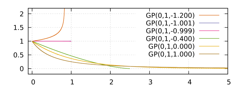
Figure 1: Generalized pareto distribution $\mathrm{GP}(0,1,\xi)$.

Theorem 3 (Pickands–Balkema–de Haan).

Let ${\textnormal{x}}_{1},\ldots{\textnormal{x}}_{n}\sim p({\textnormal{x}})$ be i.i.d. RVs defined on $X$ and ${\textnormal{x}}_{k,n}=\theta$ be their top-$k$ element. As $n\rightarrow\infty$, $k\rightarrow\infty$, $\frac{k}{n}\rightarrow 0$ ($k\ll n$), then $p({\textnormal{x}}\mid{\textnormal{x}}>\theta)\rightarrow\mathrm{GP}({\textnormal{x}}\mid\theta,\sigma,\xi)$ for some $\sigma$ and $\xi$.

$\theta$, $\sigma$ and $\xi$ are called the location, the scale and the shape parameter. It has a support ${\textnormal{x}}\in[\theta,\theta-\frac{\sigma}{\xi}]$ when $\xi<0$, otherwise ${\textnormal{x}}\in[\theta,\infty]$. The shape dictates the tail behavior: $\xi>0$ corresponds to a heavy-tailed distribution, $\xi<0$ corresponds to a short-tailed distribution, and $\xi=0$ corresponds to a shifted Exponential distribution. Pareto, Exponential, Power, and Uniform distributions (Table 1) are special cases of GP distribution. They share the characteristics that the density is 0 below a threshold $\theta$.

Special cases	$\theta$	$\sigma$	$\xi$
${\textnormal{x}}\sim\mathrm{Pa}(\alpha,l)$	$l>0$	${l}/{\alpha}$	${1}/{\alpha}>0$
${\textnormal{x}}\sim\mathrm{Lomax}(\alpha,l)$	$0$	${l}/{\alpha}$	${1}/{\alpha}>0$
${\textnormal{x}}\sim\mathrm{Exp}(\alpha,l)$	$l$	${1}/{\alpha}$	$0$
$-{\textnormal{x}}\sim\mathrm{Pow}(a,b)$	$-a<0$	${a}/{b}$	$-{1}/{b}<0$
$1/{\textnormal{x}}\sim\mathrm{iPa}(\alpha,l)$	$-{1}/{l}<0$	${1}/{l\alpha}$	$-{1}/{\alpha}<0$
${\textnormal{x}}\sim U(l,u)$	$l$	$u-l$	$-1$

Table 1: Special cases of Generalized Pareto distribution.

A typical application of GP is as follows: Given a set of time-series data $(t_{i},x_{i})$, extract a subset whose $x_{i}$ exceeds a certain sufficiently high threshold $\theta$, such as the top 5% element. Then $x_{i}$ in the subset, as well as the future exceeding data, follow a GP distribution. GP is an accurate approximation when we ignore almost all data ($\frac{k}{n}\rightarrow 0$) while retaining enough data ($k\rightarrow\infty$) as $n\rightarrow\infty$ and $\theta\rightarrow\sup X$.

Estimating the parameters of $\mathrm{GP}$ is known to be difficult. First of all, the maximum likelihood estimator (MLE) for $\sigma$ and $\xi$ of $\mathrm{GP}(0,\sigma,\xi)$ (Smith 1987) has many issues. MLE of GP does not have a closed form solution except for the solution of $\sigma$ limited to $\xi=0$. When $\xi<-1$, it does not exist because the log likelihood can reach $\infty$. It is asymptotically normal and efficient only for $\xi>-0.5$. Solving it requires a numerical method, such as the Newton-Raphson iteration. Hosking and Wallis (1987) showed that the iteration sometimes does not converge when $k$ is small or $\xi<0$, and even if it converges, the solution can be inaccurate if $k$ is small.

Due to these issues, several consistent estimators (i.e., an estimator that converges in probability to the true value as $k\rightarrow\infty$) have been developed but still with varying degrees of limitations. Hill’s estimator (Hill 1975) applies a limiting assumption to the maximum likelihood estimator in order to obtain a closed form. Smoothed Hill’s estimator (Resnick and Stărică 1997) reduces its variance. Fraga Alves (2001) addresses its location sensitivity. Method of Moments (MOM) and Probability-Weighted Moments (PWM) (Hosking and Wallis 1987) do not have the limiting assumption, have closed forms, and are more accurate, but they require $\xi<0.5$ to exist, and $\xi>0$ to be consistent, because they rely on the existence of the zeroth and the first moment (i.e., the mean and the variance). The Elemental Percentile Method (EPM) (Castillo and Hadi 1995, 1997) addresses the restriction on $\xi$ in the existing methods, but it also involves a numerical method (Newton-Raphson), and is better than MOM/PWM only when $\xi<0$.

Several Bayesian estimators are also available. Diebolt et al. (2005) proposed a Bayesian quasi-conjugate prior, but this is limited to $\xi>0$ and also requires a numerical method (Gibbs sampling). Sharpe and Juárez (2021) proposed a method based on so-called Bayesian Reference Intrinsic (BRI) approach (Bernardo and Rueda 2002). Vilar-Zanón and Lozano-Colomer (2007) proposed Generalized Inverse Gaussian distribution as a conjugate prior for Pareto distribution, again limited to $\xi>0$. Sharpe and Juárez (2021) also reproduced Vilar-Zanón and Lozano-Colomer (2007) with a simplified independence assumption and Jeffery’s improper prior.

3 Bayesian Reasoning

While existing literature focuses on the estimation of the tail index $\xi$ and the scale $\sigma$, not much focus is spent on the estimation of $\theta$. However, estimating $\theta$ is important for predicting the minimum/maximum value that a random variable can take. We are especially interested in the conjugate priors for the lower bound / threshold parameter $\theta$, as well as the upper bound $\mu-\frac{\sigma}{\xi}$ that exists when $\xi<0$ (short-tailed distribution). We also target the audience that are interested in a baseline formulation that is easy to implement, is good enough for practical applications, or when absolute accuracy can be sacrificed. We thus focus on deriving conjugate prior distributions for the special cases listed in Table 1.

We begin by the basic terminologies.

Definition 15.

Distributions $p({\textnormal{x}}_{1})=f({\textnormal{x}}_{1},\theta_{1},\ldots,\theta_{N})$ and $p({\textnormal{x}}_{2})=f({\textnormal{x}}_{2},\phi_{1},\ldots,\phi_{N})$ are of the same family if they have the same functional form $f$ only differing in the parameters $\theta_{1},\ldots,\theta_{N}$ and $\phi_{1},\ldots,\phi_{N}$.

Definition 16.

A distribution is a conjugate of another distribution when they are of the same variable and of the same family. The two distributions are then conjugates.

Example 1.

Two Gaussian distributions $p(x)={\mathcal{N}}(0,1)$ and $p(y)={\mathcal{N}}(2,3)$ are of the same family (0,1,2,3 are the parameters). $p(x)$ and $q(x)={\mathcal{N}}(4,5)$ are conjugates. $p(x)$ and $p(x|z)={\mathcal{N}}(2z+1,1)$ are also conjugates.

Convention 1.

Let $x$ be an observable RV and $z$ be a latent RV. When a prior distribution $p(z)$ is a conjugate of a posterior distribution $p(z|x)$, $p(z)$ is a conjugate prior distribution for a generative distribution $p(x|z)$.

Convention 2.

A prior distribution is informative if its parameters are chosen by the domain knowledge.

Convention 3.

A prior distribution is non-informative if its parameters are selected by the principle of maximum entropy due to the lack of such a domain knowledge.

Convention 4.

A non-informative prior is improper if the prior does not satisfy the probability axiom at the limit of entropy maximization.

In the following sections, we follow a fixed format shown below to prove each conjugate prior.

Convention 5 (Bayesian Reasoning with a single unknown parameter).

Bayesian reasoning is a form of Bayesian statistical modeling (Gelman et al. 1995) applied as follows:

1. List observable RVs: $X=(x_{1},\ldots,x_{n})$.

2. Latent RVs: A parameter $\theta$.

3. Causal dependency: Assume each observation is i.i.d. given $\theta$, i.e., $x_{i}\perp x_{j}\mid\theta$ and $p(x_{i}|\theta)=p(x_{j}|\theta)$. In other words, $p(X)=\sum_{\theta}p(\theta)\prod_{i}p(x_{i}|\theta)$.

4. Choose a distribution family and its parameters.

   1. Choose a family for $p(x_{i}|\theta)$.

   2. Write down $p(x_{i}|\theta)$.

   3. Write down $p(X|\theta)=p(x_{1},\ldots,x_{n}|\theta)=\prod_{i}p(x_{i}|\theta)$.

   4. Perform a dimensional analysis on $\theta$ and $n$ using $p(X)=\frac{p(X|\theta)p(\theta)}{p(\theta|X)}=f(\theta)\frac{p(\theta)}{p(\theta|X)}$ being constant for $\theta$. Choose a family and parameters for $p(\theta)$ and $p(\theta|X)$ based on the analysis, assuming $p(\theta)$ is parameterized by pseudocount $n_{0}$ and the prior parameter $\theta_{0}$, as well as $p(\theta|X)$ by pseudocount $n+n_{0}$ and the updated parameter $\theta_{n}$.

   5. Write down $p(\theta)$.

   6. Derive $p(\theta|X)$ and the parameter $\theta_{n}$. This is often done in one of the following manners:

      1. Use $p(\theta|X)=\frac{p(X|\theta)p(\theta)}{p(X)}\propto p(X|\theta)p(\theta)$ with $p(X)$ being constant. Ignore constant factors and match $\theta$’s coefficients in the result with the pdf of $\theta$.

      2. Derive $p(\theta,X)=p(X|\theta)p(\theta)$, then $p(X)=\int p(\theta,X)d\theta$, then $p(\theta|X)=\frac{p(\theta,X)}{p(X)}$.

5. Derive a predictive distribution $p(x|X)$ for a future data $x$ given historical data $X$. This is using the fact that $x$ does not depend on $X$ given $\theta$.

   $$p(x|X)=\int p(x|\theta,X)p(\theta|X)d\theta=\int p(x|\theta)p(\theta|X)d\theta.$$

   Using held-out data $x^{\prime}_{1},\ldots x^{\prime}_{M}$, verify the hypothesis (statistical model) made above by computing $p(X^{\prime}|X)=\prod_{i}p(x=x^{\prime}_{i}|X)$ (or, alternatively, $\log p(X^{\prime}|X)=\sum_{i}\log p(x=x^{\prime}_{i}|X)$).

6. If possible, derive an improper non-informative prior.

Finally, we derive a multi-parameter reasoning method from single-parameter reasoning methods. The goal of multi-parameter Bayesian reasoning is to obtain the joint posterior distribution of the parameters $p(\theta_{1}\ldots,\theta_{N}|X)$ and subsequently obtain the predictive distribution $p(x|X)$ to test the hypothesis. Assuming the availability of a single parameter reasoning process for each parameter of the distribution family, one should derive $p(\theta_{i}|X,\theta_{1},\ldots,\theta_{i-1})=\frac{p(X|\theta_{1},\ldots,\theta_{i-1})p(\theta_{i}|\theta_{1},\ldots,\theta_{i-1})}{p(X|\theta_{1},\ldots,\theta_{i-1})}$ for each $i$, starting from $p(\theta_{1}|X)$.

The only difference between single- and multi-parameter cases is that the process involves decomposing a more complex hierarchical model, and that it requires a joint prior distribution $p(\theta_{1}\ldots,\theta_{N})$. However, the derivation from a joint prior tends to be overly complex, therefore we sometimes use uninformative priors for mathematical convenience, as well as assuming the independence between priors, i.e., $p(\theta_{1}\ldots,\theta_{N})=p(\theta_{1})\ldots p(\theta_{N})$. Although uninformative priors are not particularly helpful/informational in the reasoning, this is not an issue because the effect/importance of the prior distributions diminishes as the depth of the model hierarchy increases.

The proofs start after the references.

4 Analytical subset for $\xi>0$: Pareto

For $l>0$ and $\alpha>0$, Pareto distribution $\mathrm{Pa}(\alpha,l)$ is a special case of $\mathrm{GP}$ as follows:

$$\mathrm{GP}{\left(l,\frac{l}{\alpha},\frac{1}{\alpha}\right)} =\frac{\alpha}{l}(1+\frac{\frac{1}{\alpha}(x-l)}{\frac{l}{\alpha}})^{-1-\alpha}=\frac{\alpha}{l}{\left(\frac{x}{l}\right)}^{-1-\alpha}$$

$$=\frac{\alpha l^{\alpha}}{x^{\alpha+1}}=\mathrm{Pa}(\alpha,l).$$

Figure 2: Pareto distribution $\mathrm{Pa}(\alpha,1)$.

Proofs for the conjugate priors were first given in Malik (1970).

4.1 Pareto with Unknown Lower Bound $l$

Example 2.

Checking laptop prices online, I found $n=20$ offers and I believe it follows $p(x_{i}|l)=\mathrm{Pa}(\alpha=1.2,l)$ for some cheapest / minimum price $l$ that I want to know. I know conservatively a laptop should cost at least $l_{0}=100$ USD, i.e., a prior assumption. Can we improve $l_{0}$ using data?

1. Latents: $l$.

2. Distribution family and parameters:

   1. $p(x_{i}|l)=\mathrm{Pa}(x_{i}|\alpha,l).\quad(0<l<x_{i})$.

   2. $p(x_{i}|l)=\alpha l^{\alpha}x_{i}^{-(\alpha+1)}$.

   3. $p(X|l)=\alpha^{n}l^{\alpha n}\prod_{i}x_{i}^{-(\alpha+1)}.\quad(0<l<\min_{i}x_{i}={\bar{l}})$

   4. The coefficients of $l$ in $p(l)$ and $p(l|X)$ differ by $l^{\alpha n}$. This matches Power distributions $\mathrm{Pow}(a,b)=\frac{bx^{b-1}}{a^{b}}$ $(0<x<a)$ with following parameters:

      $p(l)=\mathrm{Pow}(l_{0},\alpha n_{0})$ ($0<l<l_{0}$) and

      $p(l|X)=\mathrm{Pow}(l_{n},\alpha(n_{0}+n))$ ($0<l<l_{n}$).

   5. $p(l)=\alpha n_{0}l_{0}^{-\alpha n_{0}}l^{\alpha n_{0}-1}$.

   6. Using the second strategy. Let $l_{n}=\min(l_{0},{\bar{l}})$.

      $$p(l,X) =p(X|l)p(l)\quad(0<l<l_{n})$$

      $$=Al^{\alpha(n+n_{0})-1}.$$

      $$p(X) \textstyle=\int_{0}^{l_{n}}p(l,X)dl=\frac{A}{\alpha(n+n_{0})}l_{n}^{\alpha(n+n_{0})}-0.$$

      $$p(l|X) =\frac{p(l,X)}{p(X)}=\alpha(n+n_{0})l_{n}^{-\alpha(n+n_{0})}l^{\alpha(n+n_{0})-1}$$

      $$=\mathrm{Pow}(l_{n},\alpha(n_{0}+n)).$$

      In other words, the new lower bound $l_{n}$ updated from the prior lower bound $l_{0}$ is the minimum of $l_{0}$ and the empirical minimum ${\bar{\pi}}$.

3. $p(x|X)=\int_{0}^{l_{n}}p(x|l)p(l|X)dl$

   $$=\int_{0}^{l_{n}}\alpha x^{-(\alpha+1)}\alpha(n+n_{0})l_{n}^{-\alpha(n+n_{0})}l^{\alpha(n+n_{0}+1)-1}dl$$

   $$={\left<\alpha x^{-(\alpha+1)}\alpha(n+n_{0})l_{n}^{-\alpha(n+n_{0})}\frac{l^{\alpha(n+n_{0}+1)}}{\alpha(n+n_{0}+1)}\right>}_{0}^{l_{n}}$$

   $$=\alpha\frac{n+n_{0}}{n+n_{0}+1}l_{n}^{\alpha}x^{-(\alpha+1)}=\mathrm{Pa}{\left(x\mid\alpha,{\left(\frac{n+n_{0}}{n+n_{0}+1}\right)}^{\frac{1}{\alpha}}l_{n}\right)}.$$

   Notice that the new lower bound ${\left(\frac{n+n_{0}}{n+n_{0}+1}\right)}^{\frac{1}{\alpha}}l_{n}$ is smaller than the posterior lower bound $l_{n}$ or the empirical lower bound ${\bar{l}}$ because ${\left(\frac{n+n_{0}}{n+n_{0}+1}\right)}^{\frac{1}{\alpha}}<1$. Bayesian reasoning thus allows extrapolation from the data.

4. A non-informative prior is obtained by $n_{0}\rightarrow\alpha^{-1}$:

   $$p(l) \rightarrow l_{0}^{-1}:\text{Const}.$$

   $$p(l|X) \rightarrow\mathrm{Pow}(l_{n},\alpha n+1).$$

4.2 Pareto with Unknown Shape $\alpha$

Example 3.

Checking laptop prices online, I found $n=20$ offers which follow $p(x_{i}|\alpha)=\mathrm{Pa}(\alpha,l=100)$. I want to know $\alpha$ which tells the variability. I have a a prior assumption $p(\alpha)=\Gamma(2,2)$ (Gamma distribution).

1. Latents: $\alpha$.

2. Distribution family and parameters:

   1. $p(x_{i}|\alpha)=\mathrm{Pa}(x_{i}|\alpha,l).\quad(0<\alpha)$

   2. $p(x_{i}|\alpha)=\alpha l^{\alpha}x_{i}^{-(\alpha+1)}$.

   3. $p(X|\alpha)=\alpha^{n}l^{\alpha n}\prod_{i}x_{i}^{-(\alpha+1)}\quad(0<\alpha)$

      $=\alpha^{n}l^{\alpha n}l^{-n(\alpha+1)}\prod_{i}{\left(\frac{x_{i}}{l}\right)}^{-(\alpha+1)}$

      $=\alpha^{n}l^{-n}\prod_{i}{\left(\frac{x_{i}}{l}\right)}^{-(\alpha+1)}.$

      Let the geometric mean relative to $l$ be ${\bar{g}}=\prod_{i}{\left(\frac{x_{i}}{l}\right)}^{\frac{1}{n}}$.

      Then $p(X|\alpha)=\alpha^{n}l^{-n}{\bar{g}}^{-n(\alpha+1)}\propto\alpha^{n}e^{-n\log{\bar{g}}\alpha}$.

   4. The coefficients of $\alpha$ in $p(\alpha)$ and $p(\alpha|X)$ differ by $\alpha^{n}e^{-n\log{\bar{g}}\alpha}$. This matches Gamma distributions $\Gamma(a,b)\propto x^{a-1}e^{-bx}$ with following parameters:

      $p(\alpha)=\Gamma(n_{0},n_{0}\log g_{0})$ and

      $p(\alpha|X)=\Gamma(n_{0}+n,(n+n_{0})\log g_{n})$.

   5. $p(\alpha)\propto\alpha^{n_{0}-1}e^{-n_{0}\log g_{0}\alpha}=\alpha^{n_{0}-1}g_{0}^{-n_{0}\alpha}$.

   6. Using the first strategy. $p(\alpha,X)=p(X|\alpha)p(\alpha)\propto$

      $${}^{(n+n_{0})-1}{\left(g_{0}^{n_{0}}{\bar{g}}^{n}\right)}^{-\alpha} \propto\alpha^{(n+n_{0})-1}{\left(g_{n}\right)}^{-(n+n_{0})\alpha}$$

      $$\propto p(\alpha|x),$$

      where $g_{n}={\left(g_{0}^{n_{0}}{\bar{g}}^{n}\right)}^{\frac{1}{n+n_{0}}}$. In other words, the new geometric mean $g_{n}$ relative to $l$ is a geometric mean of $g_{0}$ weighted by $n_{0}$ and the empirical geometric mean ${\bar{g}}$ weighted by $n$.

      Let $A=n_{0}+n,B=(n+n_{0})\log g_{n}$.

3. Let $p(\alpha|X)=\Gamma(A,B)$.

   $$p(x,\alpha|X) \textstyle=p(x|\alpha)p(\alpha|X)$$

   $$\textstyle=\alpha l^{\alpha}x^{-(\alpha+1)}\cdot\frac{B^{A}}{\Gamma(A)}\alpha^{A-1}e^{-B\alpha}$$

   $$\textstyle=\frac{B^{A}}{x\Gamma(A)}\alpha^{A}e^{-(B+\log\frac{x}{l})\alpha}.$$

   $$p(x|X) \textstyle=\int_{0}^{\infty}p(x,\alpha|X)d\alpha$$

   $$\textstyle=\frac{B^{A}}{x\Gamma(A)}\frac{\Gamma(A+1)}{(B+\log\frac{x}{l})^{A+1}}\quad(\because\int_{0}^{\infty}x^{a}e^{-bx}dx=\frac{\Gamma(a+1)}{b^{a+1}})$$

   $$\textstyle=\frac{AB^{A}}{x(B+\log\frac{x}{l})^{A+1}}\quad(\because\Gamma(z+1)=z\Gamma(z))$$

   $$\textstyle=\frac{dy}{dx}\frac{AB^{A}}{(B+y)^{A+1}}=\frac{dy}{dx}\mathrm{Pa}(y-B|A,B).\quad(y=\log\frac{x}{l})$$

   $$\textstyle\therefore p(\log\frac{x}{l}+B|X)=\mathrm{Pa}(A,B).$$

4. A non-informative improper prior distribution is obtained by the limit of $n_{0}\downarrow 0$:

   $$p(\alpha)=\alpha^{n_{0}-1}{\left(\frac{l}{l_{0}}\right)}^{n_{0}\alpha} \xrightarrow{n_{0}\downarrow 0}\alpha^{-1}.$$

   $$p(\alpha|X) \xrightarrow{n_{0}\downarrow 0}\Gamma(n,n\log\frac{{\bar{\pi}}}{l}).$$

4.3 Pareto with Unknown $\alpha,l$

1. Latents: $l,\alpha$.

2. Distribution family and parameters:

   1. $p(x_{i}|l,\alpha)=\mathrm{Pa}(x_{i}|\alpha,l).\quad(0<l<x_{i})$.

   2. $p(x_{i}|l,\alpha)=\alpha l^{\alpha}x_{i}^{-(\alpha+1)}$.

   3. $p(X|l,\alpha)=\alpha^{n}l^{\alpha n}\prod_{i}x_{i}^{-(\alpha+1)}$.

      Let the geometric mean of data be ${\bar{g}}=\prod_{i}x_{i}^{\frac{1}{n}}$. Then $p(X|l,\alpha)=\alpha^{n}l^{\alpha n}{\bar{g}}^{-n(\alpha+1)}\propto\alpha^{n}l^{\alpha n}e^{-n\log{\bar{g}}\alpha}$.

   4. $\begin{aligned} p(l,\alpha)&=p(l|\alpha)p(\alpha)\\ &=\mathrm{Pow}(l|l_{0},\alpha n_{0})\cdot\Gamma(\alpha|n^{\prime}_{0},n^{\prime}_{0}\log g_{0}).\end{aligned}$

   5. Using the first strategy.

      $p(l|\alpha,X)p(\alpha|X)=p(l,\alpha|X)\propto p(X|l,\alpha)p(l|\alpha)p(\alpha)$

      $$\propto\alpha^{n}l^{n\alpha}e^{-n\log{\bar{g}}\alpha}p(l|\alpha)p(\alpha)$$

      $$\propto l^{n\alpha}p(l|\alpha)\cdot\alpha^{n}e^{-n\log{\bar{g}}\alpha}p(\alpha)$$

      $$\propto\mathrm{Pow}(l|l_{n},(n+n_{0})\alpha)\cdot\Gamma(\alpha|n+n^{\prime}_{0},(n+n^{\prime}_{0})\log g_{n})$$

      where $l_{n}=\min(l_{0},{\bar{l}})$, $g_{n}={\left(g_{0}^{n^{\prime}_{0}}{\bar{g}}^{n}\right)}^{\frac{1}{n+n^{\prime}_{0}}}$.

      Let $A=n^{\prime}_{0}+n,B=(n+n^{\prime}_{0})\log g_{n}$.

3. $p(x|X)=\int p(x,l,\alpha|X)dld\alpha.$

   $$p(x,l,\alpha|X)=p(x|l,\alpha)p(l|\alpha,X)p(\alpha|X)$$

   $$=\frac{\alpha l^{\alpha}}{x^{\alpha+1}}\cdot\frac{\alpha(n+n_{0})l^{\alpha(n+n_{0})-1}}{l_{n}^{\alpha(n+n_{0})}}\cdot\frac{B^{A}}{\Gamma(A)}\alpha^{A-1}e^{-B\alpha}$$

   $$=\frac{\alpha(n+n_{0})l^{\alpha(n+n_{0}+1)-1}}{l_{n}^{\alpha(n+n_{0})}}\cdot\frac{B^{A}}{x\Gamma(A)}\alpha^{A}e^{-(B+\log x)\alpha}.$$

   $$p(x,\alpha|X)=\int_{0}^{l_{n}}p(x,l,\alpha|X)dl$$

   $$=\frac{\alpha(n+n_{0})}{l_{n}^{\alpha(n+n_{0})}}\frac{l_{n}^{\alpha(n+n_{0}+1)}-0}{\alpha(n+n_{0}+1)}\cdot\frac{B^{A}}{x\Gamma(A)}\alpha^{A}e^{-(B+\log x)\alpha}$$

   $$=\frac{n+n_{0}}{n+n_{0}+1}\cdot\frac{B^{A}}{x\Gamma(A)}\alpha^{A}e^{-(B+\log\frac{x}{l_{n}})\alpha}.$$

   $$p(x|X)\textstyle=\int_{0}^{\infty}p(x,\alpha|X)d\alpha$$

   $$\textstyle=\frac{n+n_{0}}{n+n_{0}+1}\cdot\frac{B^{A}}{x\Gamma(A)}\frac{\Gamma(A+1)}{(B+\log\frac{x}{l_{n}})^{A+1}}\quad(\because\int_{0}^{\infty}x^{a}e^{-bx}dx=\frac{\Gamma(a+1)}{b^{a+1}})$$

   $$\textstyle=\frac{n+n_{0}}{n+n_{0}+1}\cdot\frac{AB^{A}}{x(B+\log\frac{x}{l_{n}})^{A+1}}\quad(\because\Gamma(z+1)=z\Gamma(z))$$

   $$\textstyle=\frac{n+n_{0}}{n+n_{0}+1}\frac{dy}{dx}\frac{AB^{A}}{y^{A+1}}.\quad(y=\log\frac{x}{l_{n}}+B)$$

   $$\textstyle\therefore p(\log\frac{x}{l_{n}}+B|X)=\mathrm{Pa}(A,{\left(\frac{n+n_{0}}{n+n_{0}+1}\right)}^{\frac{1}{A}}B).$$

   We observe a Bayesian extrapolation similar to the single-parameter case. From the lower bound of the Pareto distribution,

   $$y=\log\frac{x}{l_{n}}+B\in\left[{\left(\frac{n+n_{0}}{n+n_{0}+1}\right)}^{\frac{1}{A}}B,\quad\infty\right] =[y^{-*},\infty]$$

   $$x\in\left[l_{n}\exp B{\left({\left(\frac{n+n_{0}}{n+n_{0}+1}\right)}^{\frac{1}{A}}-1\right)},\infty\right] =[x^{-*},\infty]$$

   Since ${\left(\frac{n+n_{0}}{n+n_{0}+1}\right)}^{\frac{1}{A}}-1<0$, this lower bound $x^{-*}$ is smaller than $l_{n}$ and ${\bar{l}}$.

5 Analytical subset for $\xi=0$: Shifted Exponential

For $l>0$ and $\alpha>0$, a shifted Exponential distribution $\mathrm{Exp}(\alpha,l)$ is a special case of $\mathrm{GP}$ as follows:

$$\mathrm{GP}{\left(l,\frac{1}{\alpha},0\right)} =\alpha\exp-\frac{x-l}{\frac{1}{\alpha}}=\alpha e^{-\alpha(x-l)}=\mathrm{Exp}(\alpha,l).$$

Figure 3: Shited Exponential distribution $\mathrm{Exp}(\alpha,1)$.

5.1 Shifted Exponential with Unknown $l$

1. Latents: $l$.

2. Distribution family and parameters:

   1. $p(x_{i}|l)=\mathrm{Exp}(x_{i}|\alpha,l).\quad(l<x_{i})$.

   2. $p(x_{i}|l)=\alpha e^{-\alpha(x_{i}-l)}$.

   3. $p(X|l)=\alpha^{n}e^{-\alpha n({\bar{\mu}}-l)}\quad(l<\min_{i}x_{i}={\bar{l}})$

      where ${\bar{\mu}}=\frac{1}{n}\sum_{i}x_{i}$.

   4. The coefficients of $l$ in $p(l)$ and $p(l|X)$ differ by $e^{n\alpha l}$. This matches Log Power distributions $\mathrm{LogPow}(a,b)=be^{b(x-a)}$ ($x<a$):

      $p(l)=\mathrm{LogPow}(l_{0},\alpha n_{0})$ ($l<l_{0}$) and

      $p(l|X)=\mathrm{LogPow}(l_{n},\alpha(n+n_{0}))$ ($l<l_{n}$).

   5. $p(l)=n_{0}\alpha e^{\alpha n_{0}(l-l_{0})}$.

   6. Using the second strategy. Let $l_{n}=\min(l_{0},{\bar{l}})$.

      $$p(l,X) =p(X|l)p(l)\quad(l<l_{n})$$

      $$=Ae^{\alpha(n+n_{0})l}.$$

      $$p(X) \textstyle=\int_{-\infty}^{l_{n}}p(l,X)dl=\frac{A}{\alpha(n+n_{0})}e^{\alpha(n+n_{0})l_{n}}-0.$$

      $$p(l|X) =\frac{p(l,X)}{p(X)}=\alpha(n+n_{0})e^{\alpha(n+n_{0})(l-l_{n})}$$

      $$=\mathrm{LogPow}(l_{n},\alpha(n+n_{0})).$$

      In other words, the new lower bound $l_{n}$ updated from the prior lower bound $l_{0}$ is the minimum of $l_{0}$ and the empirical minimum ${\bar{l}}$.

3. $p(x|X)=\int_{-\infty}^{l_{n}}p(x|l)p(l|X)dl$

   $$=\int_{-\infty}^{l_{n}}\alpha e^{-\alpha(x-l)}\alpha(n+n_{0})e^{\alpha(n+n_{0})(l-l_{n})}$$

   $$=\int_{-\infty}^{l_{n}}\alpha^{2}(n+n_{0})e^{-\alpha(x+(n+n_{0})l_{n})}e^{\alpha(n+n_{0}+1)l}$$

   $$=\alpha^{2}(n+n_{0})e^{-\alpha(x+(n+n_{0})l_{n})}\frac{e^{\alpha(n+n_{0}+1)l_{n}}}{\alpha(n+n_{0}+1)}-0$$

   $$=\alpha\frac{n+n_{0}}{n+n_{0}+1}e^{-\alpha(x-l_{n})}=\alpha e^{-\alpha(x-l_{n}-\frac{1}{\alpha}\log\frac{n+n_{0}}{n+n_{0}+1})}$$

   $$=\mathrm{Exp}{\left(\alpha,l_{n}+\log{\left(\frac{n+n_{0}}{n+n_{0}+1}\right)}^{\frac{1}{\alpha}}\right)}.$$

   Notice that the new lower bound $l_{n}+\log{\left(\frac{n+n_{0}}{n+n_{0}+1}\right)}^{\frac{1}{\alpha}}$ is smaller than the posterior lower bound $l_{n}$ or the empirical lower bound ${\bar{l}}$ because ${\left(\frac{n+n_{0}}{n+n_{0}+1}\right)}^{\frac{1}{\alpha}}<1$. Bayesian reasoning thus allows extrapolation from the data.

4. A non-informative improper prior distributions is obtained by the limit of $n_{0}\downarrow 0$:

   $$p(l)\propto e^{\alpha n_{0}l} \xrightarrow{n_{0}\downarrow 0}C:\text{Const.}$$

   $$p(l|X) \xrightarrow{n_{0}\downarrow 0}\mathrm{LogPow}(\alpha n,{\bar{l}})$$

Note: When $y\sim\mathrm{Pow}(\alpha,\beta)$ ($0<y<\alpha$), then $\log y=x\sim\mathrm{LogPow}(a,b)$ ($-\infty<x<a=\log\alpha,b=\beta$). This follows from using $y=e^{x}$ and $dy=e^{x}dx$,

$$\int_{0}^{\alpha}\frac{\beta y^{\beta-1}}{\alpha^{\beta}}dy=\int_{-\infty}^{a}\frac{be^{(b-1)x}}{e^{ab}}e^{x}dx=\int_{-\infty}^{a}be^{b(x-a)}dx=1.$$

5.2 Shifted Exponential with Unknown $\alpha$

1. Latents: $\alpha$.

2. Distribution family and parameters:

   1. $p(x_{i}|\alpha)=\mathrm{Exp}(x_{i}|\alpha,l).\quad(0<\alpha)$.

   2. $p(x_{i}|\alpha)=\alpha e^{-\alpha(x_{i}-l)}$.

   3. $p(X|\alpha)=\alpha^{n}e^{-\alpha n({\bar{\mu}}-l)}\quad(0<\alpha)$

      where ${\bar{\mu}}=\frac{1}{n}\sum_{i}x_{i}$.

   4. The coefficients of $\alpha$ in $p(\alpha)$ and $p(\alpha|X)$ differ by $\alpha^{n}e^{-n({\bar{\mu}}-l)\alpha}$. This matches Gamma distributions $\Gamma(a,b)\propto x^{a-1}e^{-bx}$ with following parameters:

      $p(\alpha)=\Gamma(n_{0},n_{0}(\mu_{0}-l))$ and

      $p(\alpha|X)=\Gamma(n_{0}+n,(n+n_{0})(\mu_{n}-l))$.

   5. $p(\alpha)\propto\alpha^{n_{0}-1}e^{-n_{0}(\mu_{0}-l)\alpha}$.

   6. Using the first strategy. $p(\alpha,X)=p(X|\alpha)p(\alpha)$

      $$\textstyle\propto\alpha^{(n+n_{0})-1}e^{\alpha{\left(n_{0}(\mu_{0}-l)+n({\bar{\mu}}-l)\right)}}$$

      $$\textstyle\propto\alpha^{(n+n_{0})-1}e^{\alpha(n+n_{0})(\mu_{n}-l)}\propto\hskip 6.99997ptp(\alpha|x),$$

      where $\mu_{n}=\frac{n{\bar{\mu}}+n_{0}\mu_{0}}{n+n_{0}}$. In other words, the new mean $\mu_{n}$ is an average of $\mu_{0}$ and the empirical mean ${\bar{\mu}}$ weighted by $n_{0}$ and $n$, respectively.

      Let $A=n_{0}+n,B=(n+n_{0})(\mu_{n}-l)$.

3. Let $p(\alpha|X)=\Gamma(A,B)$.

   $$p(x,\alpha|X) \textstyle=p(x|\alpha)p(\alpha|X)$$

   $$\textstyle=\alpha e^{-\alpha(x-l)}\cdot\frac{B^{A}}{\Gamma(A)}\alpha^{A-1}e^{-B\alpha}$$

   $$\textstyle=\frac{B^{A}}{\Gamma(A)}\alpha^{A}e^{-(B+x-l)\alpha}$$

   $$p(x|X) \textstyle=\int_{0}^{\infty}p(x,\alpha|X)d\alpha$$

   $$\textstyle=\frac{B^{A}}{\Gamma(A)}\frac{\Gamma(A+1)}{(B+x-l)^{A+1}}\quad(\because\int_{0}^{\infty}x^{a}e^{-bx}dx=\frac{\Gamma(a+1)}{b^{a+1}})$$

   $$\textstyle=\frac{AB^{A}}{(B+x-l)^{A+1}}\quad(\because\Gamma(z+1)=z\Gamma(z))$$

   $$\textstyle\therefore p(x+B-l|X)=\mathrm{Pa}(A,B).$$

4. A non-informative improper prior distribution is obtained by the limit of $n_{0}\downarrow 0$:

   $$p(\alpha)=\alpha^{n_{0}-1}{\left(\frac{l}{l_{0}}\right)}^{n_{0}\alpha} \xrightarrow{n_{0}\downarrow 0}\alpha^{-1}.$$

   $$p(\alpha|X) \xrightarrow{n_{0}\downarrow 0}\Gamma(n,n({\bar{\mu}}-l)).$$

5.3 Shifted Exponential with Unknown $\alpha,l$

1. Latents: $l,\alpha$.

2. Distribution family and parameters:

   1. $p(x_{i}|l,\alpha)=\mathrm{Exp}(x_{i}|\alpha,l).$.

   2. $p(x_{i}|l,\alpha)=\alpha e^{-\alpha(x_{i}-l)}$.

   3. $p(X|l,\alpha)=\alpha^{n}e^{-\alpha n({\bar{\mu}}-l)}.$

   4. $\begin{aligned} p(l,\alpha)&=p(l|\alpha)p(\alpha)\\ &=\mathrm{LogPow}(l|l_{0},\alpha n_{0})\cdot\Gamma(\alpha|n^{\prime}_{0},n^{\prime}_{0}\mu_{0}).\end{aligned}$

   5. Using the first strategy.

      $p(l|X,\alpha)p(\alpha|X)=p(l,\alpha|X)\propto p(X|l,\alpha)p(l|\alpha)p(\alpha)$

      $$\propto\alpha^{n}e^{-\alpha n({\bar{\mu}}-l)}\cdot p(l|\alpha)p(\alpha)$$

      $$\propto e^{\alpha nl}p(l|\alpha)\cdot\alpha^{n}e^{-n{\bar{\mu}}\alpha}p(\alpha)$$

      $$\propto\mathrm{LogPow}(l|l_{n},\alpha(n+n_{0}))\cdot\Gamma(\alpha|n+n^{\prime}_{0},(n+n^{\prime}_{0})\mu_{n})$$

      where $l_{n}=\min(l_{0},{\bar{l}})$, $\mu_{n}=\frac{n^{\prime}_{0}\mu_{0}+n{\bar{\mu}}}{n^{\prime}_{0}+n}$.

      Let $A=n^{\prime}_{0}+n,B=(n+n^{\prime}_{0})\mu_{n}$.

3. $p(x|X)=\int p(x,l,\alpha|X)dld\alpha$

   $$p(x,l,\alpha|X)=p(x|l,\alpha)p(l|\alpha,X)p(\alpha|X)$$

   $$=\alpha e^{-\alpha(x-l)}\cdot\alpha(n+n_{0})e^{\alpha(n+n_{0})(l-l_{n})}\cdot\frac{B^{A}}{\Gamma(A)}\alpha^{A-1}e^{-B\alpha}$$

   $$=\alpha(n+n_{0})e^{\alpha(n+n_{0}+1)l}\cdot\frac{B^{A}}{\Gamma(A)}\alpha^{A}e^{-(B+x+(n+n_{0})l_{n})\alpha}.$$

   $$p(x,\alpha|X)=\int_{-\infty}^{l_{n}}p(x,l,\alpha|X)dl$$

   $$=\alpha(n+n_{0})\frac{e^{\alpha(n+n_{0}+1)l_{n}}-0}{\alpha(n+n_{0}+1)}\cdot\frac{B^{A}}{\Gamma(A)}\alpha^{A}e^{-(B+x+(n+n_{0})l_{n})\alpha}$$

   $$=\frac{n+n_{0}}{n+n_{0}+1}\frac{B^{A}}{\Gamma(A)}\alpha^{A}e^{-(B+x-l_{n})\alpha}.$$

   $$p(x|X)=\int_{0}^{\infty}p(x,\alpha|X)d\alpha$$

   $$\textstyle=\frac{n+n_{0}}{n+n_{0}+1}\cdot\frac{B^{A}}{\Gamma(A)}\frac{\Gamma(A+1)}{(B+x-l_{n})^{A+1}}\quad(\because\int_{0}^{\infty}x^{a}e^{-bx}dx=\frac{\Gamma(a+1)}{b^{a+1}})$$

   $$\textstyle=\frac{n+n_{0}}{n+n_{0}+1}\cdot\frac{AB^{A}}{(B+x-l_{n})^{A+1}}\quad(\because\Gamma(z+1)=z\Gamma(z))$$

   $$\textstyle\therefore p(x+B-l_{n}|X)=\mathrm{Pa}(A,{\left(\frac{n+n_{0}}{n+n_{0}+1}\right)}^{\frac{1}{A}}B).$$

   We observe a Bayesian extrapolation similar to the single-parameter case. From the lower bound of the Pareto distribution,

   $$y=x+B-l_{n}\in\left[{\left(\frac{n+n_{0}}{n+n_{0}+1}\right)}^{\frac{1}{A}}B,\infty\right] =[y^{-*},\infty]$$

   $$x\in\left[l_{n}+B{\left({\left(\frac{n+n_{0}}{n+n_{0}+1}\right)}^{\frac{1}{A}}-1\right)},\infty\right] =[x^{-*},\infty].$$

   Since ${\left(\frac{n+n_{0}}{n+n_{0}+1}\right)}^{\frac{1}{A}}-1<0$, this lower bound $x^{-*}$ is smaller than $l_{n}$ and ${\bar{l}}$.

6 Analytical subset for $\xi<0$: Reverted Power (or: Inverted Pareto)

When a RV $y$ follows a distribution $f$, its inverse $x=\frac{1}{y}$ is said to follow an inverted distribution of $f$. An Inverted Pareto $\frac{1}{y}=x\sim\mathrm{iPa}(\alpha,l)$ is thus defined from $y\sim\mathrm{Pa}(\alpha,l)$.

$$1=\int_{l}^{\infty}\mathrm{Pa}(y\mid\alpha,l)dy=\int_{l}^{\infty}\frac{\alpha l^{\alpha}}{y^{\alpha+1}}dy$$

$$=\int_{l^{-1}}^{0}\alpha l^{\alpha}x^{\alpha+1}{\left(\frac{-1}{x^{2}}dx\right)}=\int_{0}^{l^{-1}}\alpha l^{\alpha}x^{\alpha-1}dx.$$

$$l^{\alpha}x^{\alpha-1}=\mathrm{iPa}(\alpha,l)=\mathrm{Pow}(l^{-1},\alpha).\quad(0<x<l^{-1})$$

Inverted Pareto is equivalent to a Power distribution (Dallas 1976), which is defined as follows:

$$\mathrm{Pow}(a,b)=\frac{bx^{b-1}}{a^{b}}.\quad(0<x<a)$$

When a RV $y$ follows a distribution $f$, $x=-y$ is said to follow a reverted distribution of $f$. Inverted Pareto / Power is a reverted distribution of a special case of Generalized Pareto as follows:

$$\mathrm{GP}{\left(-a,\frac{a}{b},-\frac{1}{b}\right)} =\frac{b}{a}{\left(1+{\left(-\frac{1}{b}\right)}\frac{b}{a}(x-(-a))\right)}^{-1-\frac{1}{-\frac{1}{b}}}$$

$$=\frac{b(-x)^{b-1}}{a^{b}}$$

$$=\mathrm{Pow}(-x\mid a,b)=\mathrm{iPa}(-x\mid b,a^{-1}).$$

Finally, a special case of Uniform distribution with a lower support $l=0$, i.e., $U(0,u)=\frac{1}{u}$ $(0<x<u)$, is a special case of Power distribution $\mathrm{Pow}(a=u,b=1)$. Note that generally the Uniform distribution is not a special case of Power distribution. Both Uniform and Power have two parameters, and they are obtained by reducing the degree of freedom of the three parameter GP distribution by 1.

Figure 4: Power distribution $\mathrm{Pow}(3,\alpha)$.

To avoid the confusion due to the inverse and the reverse, we focus on a Power distribution in the following.

6.1 Power with Unknown Upper Bound $u$

1. Latents: $u$.

2. Distribution family and parameters:

   1. $p(x_{i}|u)=\mathrm{Pow}(x_{i}|u,\alpha).\quad(0<x_{i}<u)$

   2. $p(x_{i}|u)=\alpha u^{-\alpha}x_{i}^{\alpha-1}$.

   3. $p(X|u)=\alpha^{n}u^{-n\alpha}\prod_{i}x_{i}^{\alpha-1}.\quad(0<\max_{i}x_{i}<u)$

      Let $\max_{i}x_{i}={\bar{u}}$.

   4. The coefficients of $u$ in $p(u)$ and $p(u|X)$ differ by $u^{-n\alpha}$. This matches Pareto distributions $\mathrm{Pa}(a,b)=\frac{ab^{a}}{x^{a+1}}$ $(a<x)$ with following parameters:

      $p(u)=\mathrm{Pa}(\alpha n_{0},u_{0})$ and

      $p(u|X)=\mathrm{Pa}(\alpha(n+n_{0}),u_{n})$.

   5. $p(u)=\alpha n_{0}u_{0}^{\alpha n_{0}}u^{-(\alpha n_{0}+1)}$.

   6. Using the second strategy. Let $u_{n}=\max(u_{0},{\bar{u}})$.

      $$p(u,X) =p(X|u)p(u)\quad(u_{n}<u)$$

      $$=Au^{-\alpha(n+n_{0})-1}.$$

      $$p(X) \textstyle=\int_{u_{n}}^{\infty}p(u,X)dl=A\frac{0-u_{n}^{-\alpha(n+n_{0})}}{-\alpha(n+n_{0})}.$$

      $$p(u|X) =\frac{p(u,X)}{p(X)}=\frac{\alpha(n+n_{0})u_{n}^{\alpha(n+n_{0})}}{u^{\alpha(n+n_{0})+1}}$$

      $$=\mathrm{Pa}(\alpha(n+n_{0}),u_{n}).$$

      In other words, the new upper bound $u_{n}$ updated from the prior upper bound $u_{0}$ is the maximum of $u_{0}$ and the empirical maximum ${\bar{u}}$.

3. $p(x|X)=\int_{u_{n}}^{\infty}p(x|u)p(u|X)du$

   $$=\textstyle\int_{u_{n}}^{\infty}\alpha u^{-\alpha}x^{\alpha-1}\cdot\frac{\alpha(n+n_{0})u_{n}^{\alpha(n+n_{0})}}{u^{\alpha(n+n_{0})+1}}$$

   $$=\textstyle\int_{u_{n}}^{\infty}\alpha x^{\alpha-1}\alpha(n+n_{0})u_{n}^{\alpha(n+n_{0})}u^{-\alpha(n+n_{0}+1)-1}$$

   $$=\textstyle\alpha x^{\alpha-1}\alpha(n+n_{0})u_{n}^{\alpha(n+n_{0})}(0-\frac{u_{n}^{-\alpha(n+n_{0}+1)}}{-\alpha(n+n_{0}+1)})$$

   $$=\alpha x^{\alpha-1}\frac{n+n_{0}}{n+n_{0}+1}u_{n}^{-\alpha}$$

   $$=\mathrm{Pow}{\left(x\mid{\left(\frac{n+n_{0}}{n+n_{0}+1}\right)}^{\frac{-1}{\alpha}}u_{n},\alpha\right)}.$$

   Notice that the new upper bound ${\left(\frac{n+n_{0}}{n+n_{0}+1}\right)}^{\frac{-1}{\alpha}}u_{n}$ is larger than the posterior upper bound $u_{n}$ or the empirical upper bound ${\bar{u}}$ because ${\left(\frac{n+n_{0}}{n+n_{0}+1}\right)}^{\frac{1}{\alpha}}<1$. Bayesian reasoning thus allows extrapolation from the data.

4. A non-informative improper prior is obtained by the limit of $n_{0}\rightarrow 0$:

   $$p(u)\propto u^{-\alpha n_{0}-1} \rightarrow u^{-1}.$$

   $$p(u|X) \rightarrow\mathrm{Pa}(\alpha n,{\bar{u}})$$

6.2 Power with Unknown Rate $\alpha$

1. Latents: $\alpha$.

2. Distribution family and parameters:

   1. $p(x_{i}|\alpha)=\mathrm{Pow}(x_{i}|u,\alpha).\quad(\alpha>-1)$

   2. $p(x_{i}|\alpha)=\alpha u^{-\alpha}x_{i}^{\alpha-1}$.

   3. $p(X|\alpha)=\alpha^{n}u^{-n\alpha}\prod_{i}x_{i}^{\alpha-1}.\quad(\alpha>-1)$

      $=\alpha^{n}u^{-n\alpha}u^{n(\alpha-1)}\prod_{i}{\left(\frac{x_{i}}{u}\right)}^{\alpha-1}$

      $=\alpha^{n}u^{-n}\prod_{i}{\left(\frac{x_{i}}{u}\right)}^{\alpha-1}$.

      Let the geometric mean of the data relative to $u$ be ${\bar{g}}=\prod_{i}{\left(\frac{x_{i}}{u}\right)}^{\frac{1}{n}}$. Then $p(X|\alpha)\propto\alpha^{n}{\bar{g}}^{n(\alpha-1)}\propto\alpha^{n}e^{n\log{\bar{g}}\alpha}$.

   4. The coefficients of $\alpha$ in $p(\alpha)$ and $p(\alpha|X)$ differ by $\alpha^{n}e^{n\log{\bar{g}}\alpha}$. This matches Gamma distributions $\Gamma(a,b)\propto x^{a-1}e^{-bx}$ with following parameters:

      $p(\alpha)=\Gamma(n_{0},-n_{0}\log g_{0})$ and

      $p(\alpha|X)=\Gamma(n_{0}+n,-(n+n_{0})\log g_{n})$.

   5. $p(\alpha)\propto\alpha^{n_{0}-1}e^{n_{0}\log g_{0}\alpha}=\alpha^{n_{0}-1}g_{0}^{n_{0}\alpha}$.

   6. Using the first strategy. $p(\alpha,X)=p(X|\alpha)p(\alpha)\propto$ $\alpha^{(n+n_{0})-1}{\left(g_{0}^{n_{0}}{\bar{g}}^{n}\right)}^{\alpha}\propto\alpha^{(n+n_{0})-1}g_{n}^{(n+n_{0})\alpha}\propto\hskip 6.99997ptp(\alpha|x)$, where $g_{n}={\left(g_{0}^{n_{0}}{\bar{g}}^{n}\right)}^{\frac{1}{n+n_{0}}}$. In other words, the new rate relative to $u$ is a geometric mean of $g_{0}$ weighted by $n_{0}$ and the empirical geometric mean ${\bar{g}}$ weighted by $n$.

3. Let $p(\alpha|X)=\Gamma(A,B)$. $B>0$ because $g_{n}<1$.

   $$p(x,\alpha|X) \textstyle=p(x|\alpha)p(\alpha|X)$$

   $$\textstyle=\alpha u^{-\alpha}x^{\alpha-1}\cdot\frac{B^{A}}{\Gamma(A)}\alpha^{A-1}e^{-B\alpha}$$

   $$\textstyle=\frac{B^{A}}{x\Gamma(A)}\alpha^{A}e^{-(B+\log\frac{u}{x})\alpha}$$

   $$p(x|X) \textstyle=\int_{0}^{\infty}p(x,\alpha|X)d\alpha$$

   $$\textstyle=\frac{B^{A}}{x\Gamma(A)}\frac{\Gamma(A+1)}{(B+\log\frac{u}{x})^{A+1}}\quad(\because\int_{0}^{\infty}x^{a}e^{-bx}dx=\frac{\Gamma(a+1)}{b^{a+1}})$$

   $$\textstyle=\frac{AB^{A}}{x(B+\log\frac{u}{x})^{A+1}}\quad(\because\Gamma(z+1)=z\Gamma(z))$$

   $$\textstyle=\frac{dy}{dx}\frac{AB^{A}}{(B-y)^{A+1}}=\frac{dy}{dx}\mathrm{Lomax}(-y|A,B).\quad(y=\log\frac{x}{u})$$

   $$\textstyle\therefore p(-\log\frac{x}{u}+B|X)=\mathrm{Pa}(A,B).$$

4. A non-informative improper prior distributions is obtained by the limit of $n_{0}\downarrow 0$:

   $$p(\alpha)=\alpha^{n_{0}-1}{\left(\frac{u_{0}}{u}\right)}^{n_{0}\alpha} \xrightarrow{n_{0}\downarrow 0}\alpha^{-1}.$$

   $$p(\alpha|X) \xrightarrow{n_{0}\downarrow 0}\Gamma(n,n\log\frac{u}{{\bar{g}}}).$$

6.3 Power with Unknown $\alpha,u$

1. Latents: $u,\alpha$.

2. Distribution family and parameters:

   1. $p(x_{i}|u,\alpha)=\mathrm{Pow}(x_{i}|u,\alpha).$

   2. $p(x_{i}|u,\alpha)=\alpha u^{-\alpha}x_{i}^{\alpha-1}$.

   3. $p(X|u,\alpha)=\alpha^{n}u^{-\alpha n}\prod_{i}x_{i}^{\alpha-1}$.

      Let the geometric mean of data be ${\bar{g}}=\prod_{i}x_{i}^{\frac{1}{n}}$. Then

      $p(X|u,\alpha)=\alpha^{n}u^{-n\alpha}{\bar{g}}^{n(\alpha-1)}\propto\alpha^{n}u^{-n\alpha}e^{n\log{\bar{g}}\alpha}.$

   4. $\begin{aligned} p(u,\alpha)&=p(u|\alpha)p(\alpha)\\ &=\mathrm{Pa}(u|\alpha n_{0},u_{0})\cdot\Gamma(\alpha|n^{\prime}_{0},-n^{\prime}_{0}\log g_{0})\\ \end{aligned}$

   5. $p(u|X,\alpha)p(\alpha|x)=p(u,\alpha|X)\propto p(X|u,\alpha)p(u|\alpha)p(\alpha)$

      $$\propto\alpha^{n}e^{n\log{\bar{g}}\alpha}u^{-n\alpha}\cdot p(u|\alpha)p(\alpha)$$

      $$\propto u^{-n\alpha}p(u|\alpha)\cdot\alpha^{n}e^{n\log{\bar{g}}\alpha}p(\alpha)$$

      $$\propto\mathrm{Pa}(u|\alpha(n+n_{0}),u_{n})\cdot\Gamma(\alpha|n+n^{\prime}_{0},-(n+n^{\prime}_{0})\log g_{n}),$$

      where $u_{n}=\max(u_{0},\max_{i}x_{i})$, $g_{n}=(g_{0}^{n_{0}}{\bar{g}}^{n})^{\frac{1}{n+n_{0}}}.$

      Let $A=n+n^{\prime}_{0},B=-(n+n^{\prime}_{0})\log g_{n}$.

3. $p(x|X)=\int p(x,u,\alpha|X)dud\alpha$

   $$p(x,u,\alpha|X)=p(x|u,\alpha)p(u|\alpha,X)p(\alpha|X)$$

   $$=\frac{\alpha x^{\alpha-1}}{u^{\alpha}}\cdot\frac{\alpha(n+n_{0})u_{n}^{\alpha(n+n_{0})}}{u^{\alpha(n+n_{0})+1}}\cdot\frac{B^{A}}{\Gamma(A)}\alpha^{A-1}e^{-B\alpha}$$

   $$=\frac{\alpha(n+n_{0})u_{n}^{\alpha(n+n_{0})}}{u^{\alpha(n+n_{0}+1)+1}}\cdot\frac{B^{A}}{x\Gamma(A)}\alpha^{A}e^{-(B-\log x)\alpha}$$

   $$p(x,\alpha|X)=\int_{u_{n}}^{\infty}p(x,u,\alpha|X)du$$

   $$=\alpha(n+n_{0})u_{n}^{\alpha(n+n_{0})}\frac{0-u_{n}^{-\alpha(n+n_{0}+1)}}{-\alpha(n+n_{0}+1)}\cdot\frac{B^{A}}{x\Gamma(A)}\alpha^{A}e^{-(B-\log x)\alpha}$$

   $$=\frac{n+n_{0}}{n+n_{0}+1}\cdot\frac{B^{A}}{x\Gamma(A)}\alpha^{A}e^{-(B+\log\frac{u_{n}}{x})\alpha}$$

   $$p(x|X)=\int_{0}^{\infty}p(x,\alpha|X)d\alpha$$

   $$\textstyle=\frac{n+n_{0}}{n+n_{0}+1}\frac{B^{A}}{x\Gamma(A)}\frac{\Gamma(A+1)}{(B+\log\frac{u_{n}}{x})^{A+1}}\quad(\because\int_{0}^{\infty}x^{a}e^{-bx}dx=\frac{\Gamma(a+1)}{b^{a+1}})$$

   $$\textstyle=\frac{n+n_{0}}{n+n_{0}+1}\frac{AB^{A}}{x(B+\log\frac{u_{n}}{x})^{A+1}}\quad(\because\Gamma(z+1)=z\Gamma(z))$$

   $$\textstyle=\frac{n+n_{0}}{n+n_{0}+1}\frac{-dy}{dx}\frac{AB^{A}}{y^{A+1}}.\quad(y=\log\frac{u_{n}}{x}+B)$$

   $$\textstyle\therefore p(\log\frac{u_{n}}{x}+B|X)=\mathrm{Pa}(A,{\left(\frac{n+n_{0}}{n+n_{0}+1}\right)}^{\frac{1}{A}}B).$$

   The support is

   $$\begin{array}[]{cl}y=\log\frac{u_{n}}{x}+B\in\left[{\left(\frac{n+n_{0}}{n+n_{0}+1}\right)}^{\frac{1}{A}}B,\quad\infty\right]&=[y^{-*},\infty]\\ x\in\left[0,\quad u_{n}\exp-B{\left({\left(\frac{n+n_{0}}{n+n_{0}+1}\right)}^{\frac{1}{A}}-1\right)}\right]&=[0,x^{*}].\end{array}$$

   The expected value of $x$ is ${\mathbb{E}}_{p(x|X)}[x]=$

   $$\textstyle=\frac{n+n_{0}}{n+n_{0}+1}\int_{0}^{x^{*}}\ldots dx\textstyle=\frac{n+n_{0}}{n+n_{0}+1}\int_{\infty}^{y^{*}}x\frac{-dy}{dx}\frac{AB^{A}}{y^{A+1}}dy$$

   $$\textstyle=\frac{n+n_{0}}{n+n_{0}+1}\int_{y^{*}}^{\infty}u_{n}e^{B-y}\frac{AB^{A}}{y^{A+1}}dy$$

   $$\textstyle=\frac{n+n_{0}}{n+n_{0}+1}u_{n}AB^{A}e^{B}\int_{y^{*}}^{\infty}y^{-A-1}e^{-y}dy$$

   $$\textstyle=\frac{n+n_{0}}{n+n_{0}+1}u_{n}AB^{A}e^{B}\Gamma(-A,y^{*}).\quad(\text{Incomplete $\Gamma$ function}.)$$

7 Analytical subset for $\xi=-1$: Uniform

We consider the uniform distribution as a special case of $\mathrm{GP}$.

$$\mathrm{GP}{\left(l,u-l,-1\right)} =\frac{1}{u-l}{\left(1+(-1)\frac{x-l}{u-l}\right)}^{-1-\frac{1}{-1}}$$

$$=\frac{1}{u-l}.$$

Since $\xi=-1<0$, it has a support $l<x<l-\frac{u-l}{-1}=u$. This matches the uniform distribution.

Note that Pareto and Power reduces the degree of freedom in $\mathrm{GP}$ by tying $\sigma$ to $\theta$ and $\xi$, while Shifted Exponential and Uniform do so by setting $\xi$ to a specific value.

7.1 Uniform $U(l,u=l+w)$ with Unknown Width $w$

Example 4 (German Tank Problem).

The Allies have captured $N=100$ Nazi tanks each of which has a serial number painted on the side, starting from $l=1$. Currently, the maximum number observed so far is ${\bar{u}}=993$. Assuming that the number is assigned uniformly, how many tanks were likely produced?

1. Latents: $w$.

2. Distribution family and parameters:

   1. $p(x_{i}|w)=U(x_{i}|l,l+w).\quad(w>0)$

   2. $p(w)=\mathrm{Pa}(n_{0},w_{0})$.

   3. $p(w|X)=\mathrm{Pa}(n_{0}+n,w_{n})$.

3. $p(x_{i}|w)=w^{-1}$, $l<x_{i}<l+w$.

4. $p(X|w)=w^{-n}$, $l<\min_{i}x_{i}<\max_{i}x_{i}<l+w$.

   Let ${\bar{w}}=\max_{i}x_{i}-l$.

5. $p(w)=n_{0}u_{0}^{n_{0}}w^{-n_{0}-1}$ where $0<w_{0}<w$, otherwise 0.

6. Using the second strategy. $p(w,X)=p(X|w)p(w)=n_{0}u_{0}^{n_{0}}w^{-n-n_{0}-1}$ where $0<\max(w_{0},{\bar{w}})<w$, otherwise 0. Let $w_{n}=\max(w_{0},{\bar{w}})$.

   $$p(X) \textstyle=\int_{\mathbb{R}}p(w,X)dw\textstyle=\int_{w_{n}}^{\infty}p(w,X)dw$$

   $$\textstyle={\left<n_{0}u_{0}^{n_{0}}\frac{w^{-n-n_{0}}}{-n-n_{0}}\right>}_{w_{n}}^{\infty}\textstyle=\frac{n_{0}u_{0}^{n_{0}}}{n+n_{0}}w_{n}^{-n-n_{0}}.$$

   $$p(w|X) =\frac{p(w,X)}{p(X)}=\frac{(n+n_{0})w_{n}^{n+n_{0}}}{w^{(n+n_{0})+1}}=\mathrm{Pa}(n_{0}+n,w_{n}).$$

   In other words, the new max $w_{n}$ updated from the prior max $w_{0}$ is the max of $w_{0}$ and the empirical max width ${\bar{w}}$.

7. $p(x|w)p(w|X)=\frac{(n+n_{0})w_{n}^{n+n_{0}}}{w^{(n+n_{0})+2}}$.

   $$p(x|X) =\int_{w_{n}}^{\infty}p(x,w|X)dw=\int_{w_{n}}^{\infty}p(x|w)p(w|X)dw$$

   $$=0-\frac{(n+n_{0})w_{n}^{n+n_{0}}}{-(n+n_{0}+1)w_{n}^{(n+n_{0})+1}}.$$

   $$=\frac{n+n_{0}}{n+n_{0}+1}w_{n}^{-1}$$

   $$=U{\left(l,l+\frac{n+n_{0}+1}{n+n_{0}}w_{n}\right)}.$$

   Note that the updated uniform posterior predictive distribution has a wider range than the empirical distribution $U(l,l+w_{n})$, thus “has the ability to extrapolate from the data” (Tenenbaum 1998).

8. A non-informative improper prior is obtained by $n_{0}\downarrow 0$:

   $$p(w)\sim w^{-n_{0}-1} \xrightarrow{n_{0}\downarrow 0}w^{-1}.$$

   $$p(w|X)=\mathrm{Pa}(n_{0}+n,w_{n}) \xrightarrow{n_{0}\downarrow 0}\mathrm{Pa}(n,w_{n}).$$

7.2 Uniform $U(l,u=l+w)$ with Unknown Lower Bound $l$

Example 5.

The Allies have captured $N=100$ latest Nazi tanks each of which has a serial number painted on the side. We know they produced $u=10000$ tanks in total. The minimum number on these latest tanks that we observed so far is ${\bar{l}}=1945$. When did they stop producing the older version?

1. Latents: $l$.

2. Distribution family and parameters:

   1. $p(x_{i}|l)=U(x_{i}|l,l+w).\quad(w>0)$

   2. $p(l)=U(u_{0}-w,l_{0}).\quad(u_{0}-w<l<l_{0})$.

   3. $p(l|X)=U(u_{n}-w,l_{n})$.

3. $p(x_{i}|l)=w^{-1}$, $l<x_{i}<l+w$.

4. $p(X|l)=w^{-n}$, $l<\min_{i}x_{i}<\max_{i}x_{i}<l+w$.

   Let ${\bar{u}}=\max_{i}x_{i}$ and ${\bar{l}}=\min_{i}x_{i}$. Then ${\bar{u}}-w<l<{\bar{l}}$.

5. $p(l)=(l_{0}-u_{0}+w)^{-1}$.

6. Using the second strategy. $p(l,X)=p(X|l)p(l)=\text{Const}.$ where $\max(u_{0},{\bar{u}})-w<l<\min(l_{0},{\bar{l}})$, otherwise 0. Let $u_{n}=\max(u_{0},{\bar{u}})$, $l_{n}=\min(l_{0},{\bar{l}})$.

   $$p(X) \textstyle=\int_{\mathbb{R}}p(l,X)dl\textstyle=\int_{u_{n}-w}^{l_{n}}p(l,X)dl$$

   $$\textstyle={\left<w^{-n}(l_{0}-u_{0}+w)^{-1}\cdot l\right>}_{u_{n}-w}^{l_{n}}\textstyle=w^{-n}\frac{l_{n}-u_{n}+w}{l_{0}-u_{0}+w}.$$

   $$p(l|X) =\frac{p(l,X)}{p(X)}=(l_{n}-u_{n}+w)^{-1}=U(u_{n}-w,l_{n}).$$

7. $p(x,l|X)=p(x|l)p(l|X)=w^{-1}(l_{n}-u_{n}+w)^{-1}.$ Note that $l<x<l+w$ for $p(x|l)$, thus $x-w<l<x$. Therefore

   $$p(x|X) =\int_{\max(u_{n},x)-w}^{\min(l_{n},x)}p(x,l|X)dl$$

   $$=\frac{\min(l_{n},x)-\max(u_{n},x)+w}{w(l_{n}-u_{n}+w)}$$

   $$=\left\{\begin{array}[]{cl}\frac{l_{n}-x+w}{w(l_{n}-u_{n}+w)},&(l_{n}<x\land u_{n}<x\Leftrightarrow\max(l_{n},u_{n})<x)\\ w^{-1},&(l_{n}>x\land u_{n}<x\Rightarrow u_{n}<l_{n}\Rightarrow\bot)\\ \frac{l_{n}-u_{n}}{w(l_{n}-u_{n}+w)},&(l_{n}<x\land u_{n}>x\Leftrightarrow l_{n}<x<u_{n})\\ \frac{x-u_{n}+w}{w(l_{n}-u_{n}+w)}.&(l_{n}>x\land u_{n}>x\Leftrightarrow x<\min(l_{n},u_{n}))\end{array}\right.$$

   Using $p(x|X)\geq 0$,

   $$p(x|X) =\left\{\begin{array}[]{cc}\frac{l_{n}-x+w}{w(l_{n}-u_{n}+w)},&(\max(l_{n},u_{n})<x<l_{n}+w)\\ \frac{l_{n}-u_{n}}{w(l_{n}-u_{n}+w)},&(l_{n}<x<u_{n})\\ \frac{x-u_{n}+w}{w(l_{n}-u_{n}+w)}.&(u_{n}-w<x<\min(l_{n},u_{n}))\end{array}\right.$$

   This predictive distribution has a trapezoidal shape and, as usual, has a support wider than the empirical distribution $U(l_{n},u_{n})$.

8. A non-informative improper prior is obtained by $l_{0}\rightarrow-\infty,u_{0}\rightarrow\infty$.

7.3 Uniform $U(l,u=l+w)$ with Unknown $l,w$

1. Latents: $l,w$.

2. Distribution family and parameters:

   1. $p(x_{i}|l,w)=U(x_{i}|l,l+w).\quad(w>0)$

   2. $p(w)=\mathrm{Pa}(w|n_{0},w_{0}),\quad(w_{0}<w)$

      $p(l|w)=U(l|u_{0}-w,l_{0}).\quad(u_{0}-w<l<l_{0})$

3. $p(x_{i}|l,w)=w^{-1}$, $l<x_{i}<l+w$.

4. $p(X|l,w)=w^{-n}$, $l<\min_{i}x_{i}<\max_{i}x_{i}<l+w$.

   Let ${\bar{u}}=\max_{i}x_{i}$, ${\bar{l}}=\min_{i}x_{i}$, ${\bar{w}}={\bar{u}}-{\bar{l}}$.

   Then ${\bar{u}}-w<l<{\bar{l}}$ and ${\bar{w}}<w$.

5. $p(l,w)=p(l|w)p(w)=(l_{0}-u_{0}+w)^{-1}\cdot n_{0}w_{0}^{n_{0}}w^{-n_{0}-1}$

   $=(l_{0}-u_{0}+w)^{-1}\cdot Aw^{-n_{0}-1}.\quad(A=n_{0}w_{0}^{n_{0}})$

6. Using the second strategy.

   Let $u_{n}=\max(u_{0},{\bar{u}})$, $l_{n}=\min(l_{0},{\bar{l}})$, $w_{n}=u_{n}-l_{n}$. (This implies $w_{0}=u_{0}-l_{0}$, but this is rather accidental.)

   $$p(l,w,X) =p(X|l,w)p(l|w)p(w)$$

   $$=w^{-n}\cdot(w-w_{0})^{-1}\cdot Aw^{-n_{0}-1}$$

   $$=Aw^{-(n+n_{0}+1)}(w-w_{0})^{-1}.$$

   $$p(w,X) =\int_{u_{n}-w}^{l_{n}}p(l,w,X)dl=Aw^{-(n+n_{0}+1)}\frac{w-w_{n}}{w-w_{0}}.$$

   $$p(l|w,X) =\frac{p(l,w,X)}{p(w,X)}={\left(w-w_{n}\right)}^{-1}=U(l|u_{n}-w,l_{n}).$$

   Let $z=w^{-1}$, $z_{n}=w_{n}^{-1}$, $w\in[w_{n},\infty]$, $z\in[0,z_{n}]$, $N=n+n_{0}$. Then $p(X)=\int_{w_{n}}^{\infty}p(w,X)dw$

   $$\textstyle=\int_{z_{n}}^{0}Az^{N+1}\frac{z^{-1}-z_{n}^{-1}}{z^{-1}-z_{0}^{-1}}{\left(\frac{dz}{-z^{2}}\right)}\textstyle=\int_{z_{n}}^{0}-Az^{N-1}\frac{z-z_{n}}{z-z_{0}}\frac{-zz_{0}}{-zz_{n}}dz$$

   $$\textstyle=\int_{0}^{z_{n}}{\left(\frac{z^{N}}{z-z_{0}}-\frac{z_{n}z^{N-1}}{z-z_{0}}\right)}A\frac{z_{0}}{z_{n}}dz\textstyle=\int_{0}^{\frac{z_{n}}{z_{0}}}{\left(\frac{z_{0}}{z_{n}}\frac{t^{N}}{1-t}-\frac{t^{N-1}}{1-t}\right)}A\frac{z_{0}^{N}}{z_{n}}dt$$

   $$\textstyle={\left(\frac{z_{0}}{z_{n}}{\left(\frac{z_{n}}{z_{0}};N+1,0\right)}-{\left(\frac{z_{n}}{z_{0}};N,0\right)}\right)}A\frac{z_{0}^{N}}{z_{n}}$$

   $$\textstyle={\left(\frac{w_{n}}{w_{0}}{\left(\frac{w_{0}}{w_{n}};N+1,0\right)}-{\left(\frac{w_{0}}{w_{n}};N,0\right)}\right)}A\frac{w_{n}}{w_{0}^{N}}\textstyle=AC(N).$$

   $$\textstyle p(w|X)=\frac{p(w,X)}{p(X)}=w^{-(N+1)}\frac{w-w_{n}}{w-w_{0}}C(N)^{-1}.$$

   Note that the posterior $p(w|X)$ is not conjugate with $p(w)=\mathrm{Pa}(w|n_{0},w_{0})$. However, as we see below, this does not affect the posterior predictive $p(x|X)$.

7. $p(x|X)=\iint p(x|w,l)p(l|w,X)p(w|X)dldw$

   $$\textstyle=\iint w^{-1}\cdot(w-w_{n})^{-1}\cdot w^{-(N+1)}\frac{w-w_{n}}{w-w_{0}}C(N)^{-1}dldw$$

   $$\textstyle=\iint\frac{w^{-(N+2)}}{w-w_{0}}C(N)^{-1}dldw\textstyle=\int w^{-(N+2)}\frac{w-w_{n}}{w-w_{0}}C(N)^{-1}dw$$

   $$\textstyle=\frac{C(N+1)}{C(N)}=U(x|u_{n}-\frac{C(N+1)}{C(N)},u_{n}).$$

   $$\textstyle\frac{C(N+1)}{C(N)}=w_{0}^{-1}\frac{\frac{w_{n}}{w_{0}}{\left(\frac{w_{0}}{w_{n}};N+2,0\right)}-{\left(\frac{w_{0}}{w_{n}};N+1,0\right)}}{\frac{w_{n}}{w_{0}}{\left(\frac{w_{0}}{w_{n}};N+1,0\right)}-{\left(\frac{w_{0}}{w_{n}};N,0\right)}}.$$

References

- Balkema and De Haan (1974) Balkema, A. A.; and De Haan, L. 1974. Residual Life Time at Great Age. Annals of Probability, 2(5): 792–804.
- Beirlant et al. (2004) Beirlant, J.; Goegebeur, Y.; Segers, J.; and Teugels, J. L. 2004. Statistics of Extremes: Theory and Applications, volume 558. John Wiley & Sons.
- Bernardo and Rueda (2002) Bernardo, J. M.; and Rueda, R. 2002. Bayesian Hypothesis Testing: A Reference Approach. International Statistical Review, 70(3): 351–372.
- Castillo and Hadi (1995) Castillo, E.; and Hadi, A. S. 1995. A Method for Estimating Parameters and Quantiles of Distributions of Continuous Random Variables. Computational statistics & data analysis, 20(4): 421–439.
- Castillo and Hadi (1997) Castillo, E.; and Hadi, A. S. 1997. Fitting the Generalized Pareto Distribution to Data. Journal of the American Statistical Association, 92(440): 1609–1620.
- Dallas (1976) Dallas, A. 1976. Characterizing the Pareto and Power Distributions. Annals of the Institute of Statistical Mathematics, 28(1): 491–497.
- Davies (2013) Davies, J. 2013. Solving MAXSAT by decoupling optimization and satisfaction. Ph.D. thesis, University of Toronto.
- De Haan and Ferreira (2006) De Haan, L.; and Ferreira, A. 2006. Extreme Value Theory: An Introduction. Springer Science & Business Media.
- Diebolt et al. (2005) Diebolt, J.; El-Aroui, M.-A.; Garrido, M.; and Girard, S. 2005. Quasi-Conjugate Bayes Estimates for GPD Parameters and Application to Heavy Tails Modelling. Extremes, 8(1): 57–78.
- Fisher and Tippett (1928) Fisher, R. A.; and Tippett, L. H. C. 1928. Limiting Forms of the Frequency Distribution of the Largest or Smallest Member of a Sample. Mathematical Proceedings of the Cambridge Philosophical Society, 24(2): 180–190.
- Fraga Alves (2001) Fraga Alves, M. 2001. A Location Invariant Hill-Type Estimator. Extremes, 4(3): 199–217.
- Gelman et al. (1995) Gelman, A.; Carlin, J. B.; Stern, H. S.; and Rubin, D. B. 1995. Bayesian Data Analysis. Chapman and Hall/CRC.
- Gnedenko (1943) Gnedenko, B. 1943. Sur La Distribution Limite Du Terme Maximum D’Une Serie Aleatoire. Annals of Mathematics, 44(3): 423–453.
- Haslum et al. (2019) Haslum, P.; Lipovetzky, N.; Magazzeni, D.; and Muise, C. 2019. An Introduction to the Planning Domain Definition Language. Synthesis Lectures on Artificial Intelligence and Machine Learning. Morgan & Claypool Publishers.
- Hill (1975) Hill, B. M. 1975. A Simple General Approach to Inference about the Tail of a Distribution. Annals of Statistics, 1163–1174.
- Hosking and Wallis (1987) Hosking, J. R.; and Wallis, J. R. 1987. Parameter and Quantile Estimation for the Generalized Pareto Distribution. Technometrics, 29(3): 339–349.
- Laplace (1812) Laplace, P.-S. 1812. Théorie analytique des probabilités.
- Malik (1970) Malik, H. J. 1970. Estimation of the Parameters of the Pareto Distribution. Metrika, 15(1): 126–132.
- Pickands III (1975) Pickands III, J. 1975. Statistical Inference using Extreme Order Statistics. Annals of Statistics, 119–131.
- Ramesh et al. (2022) Ramesh, A.; Dhariwal, P.; Nichol, A.; Chu, C.; and Chen, M. 2022. Hierarchical Text-Conditional Image Generation with Clip Latents. arXiv preprint arXiv:2204.06125.
- Ramesh et al. (2021) Ramesh, A.; Pavlov, M.; Goh, G.; Gray, S.; Voss, C.; Radford, A.; Chen, M.; and Sutskever, I. 2021. Zero-shot text-to-image generation. In Proc. of the International Conference on Machine Learning (ICML), 8821–8831. PMLR.
- Resnick and Stărică (1997) Resnick, S.; and Stărică, C. 1997. Smoothing the Hill estimator. Advances in Applied Probability, 29(1): 271–293.
- Sharpe and Juárez (2021) Sharpe, J.; and Juárez, M. A. 2021. Estimation of the Pareto and Related Distributions–A Reference-Intrinsic Approach. Communications in Statistics-Theory and Methods, 1–23.
- Smith (1987) Smith, R. L. 1987. Estimating Tails of Probability Distributions. Annals of Statistics, 1174–1207.
- Tenenbaum (1998) Tenenbaum, J. B. 1998. Bayesian Modeling of Human Concept Learning. In NIPS, volume 11.
- Vilar-Zanón and Lozano-Colomer (2007) Vilar-Zanón, J. L.; and Lozano-Colomer, C. 2007. On Pareto Conjugate Priors and Their Application to Large Claims Reinsurance Premium Calculation. ASTIN Bulletin: The Journal of the IAA, 37(2): 405–428.