Autofluorescence Bronchoscopy Video Analysis
for Lesion Frame Detection*

Abstract

Because of the significance of bronchial lesions as indicators of early lung cancer and squamous cell carcinoma, a critical need exists for early detection of bronchial lesions. Autofluorescence bronchoscopy (AFB) is a primary modality used for bronchial lesion detection, as it shows high sensitivity to suspicious lesions. The physician, however, must interactively browse a long video stream to locate lesions, making the search exceedingly tedious and error prone. Unfortunately, limited research has explored the use of automated AFB video analysis for efficient lesion detection. We propose a robust automatic AFB analysis approach that distinguishes informative and uninformative AFB video frames in a video. In addition, for the informative frames, we determine the frames containing potential lesions and delineate candidate lesion regions. Our approach draws upon a combination of computer-based image analysis, machine learning, and deep learning. Thus, the analysis of an AFB video stream becomes more tractable. Tests with patient AFB video indicate that $\geq$97% of frames were correctly labeled as informative or uninformative. In addition, $\geq$97% of lesion frames were correctly identified, with false positive and false negative rates $\leq$3%.

Clinical relevance—The method makes AFB-based bronchial lesion analysis more efficient, thereby helping to advance the goal of better early lung cancer detection.

I INTRODUCTION

Lung cancer remains the world’s leading cause of cancer death [1]. Lung cancer begins when lesions develop in the bronchial epithelium of the lung mucosa (thin walls of the airways). Such bronchial lesions can eventually evolve into squamous cell carcinoma and possibly indicate the growth of other more distant lung tumors [2]. This motivates a new trend toward early detection of bronchial lesions and also partly drives the search for biomarkers signaling lung cancer risk [2, 3]. Physicians use bronchoscopy to search the airways for such lesions [4, 5]. A primary modality for lesion detection is autofluorescence bronchoscopy (AFB), which transmits a light source that helps measure fluorescence and absorption characteristics of airway wall tissue [5]. In particular, AFB highlights differences between the normal epithelium and developing epithelial lesions. Unlike standard white-light bronchoscopy, AFB exhibits high sensitivity to suspicious bronchial lesions. Thus, AFB figures prominently in several recent multi-center early-detection studies [6].

Current usage of AFB forces the physician to search for lesions in a long, redundant video stream and rely on interactive visual criteria to detect lesions [4, 5, 7]. Because a video stream contains thousands of frames, the search is an impractical, highly time-consuming, error-prone task. In particular, a typical video stream contains a high percentage of misleading uninformative frames, obscured by water, mucus, and motion blur. Other uninformative frames are degraded by overexposure, as when the bronchoscope is too close to an airway wall. While a few works have applied computer-based analysis to AFB video, they all have severe limitations [8, 9, 10, 11]: 1) don’t distinguish informative and uninformative frames; 2) require manual interaction to identify a lesion frame; and 3) entail manual interaction to define a lesion.

We propose a automatic AFB analysis approach, drawing upon computer-based image analysis, machine learning, and deep learning to detect informative AFB video frames in a video stream. Furthermore, for those frames deemed informative, our approach determines which frames contain potential bronchial lesions and delineates candidate lesion regions. In this way, the analysis of a long AFB video stream becomes more practical and helps focus subsequent detailed classification. Tests with human lung-cancer patient data demonstrate the efficacy of our approach.

II METHODS

Given a true-color three-channel RGB AFB video frame ${\bf I}$ (frame size = 720$\times$720 pixels (HD) or 360$\times$360 pixels (SD)), our method has three stages: (1) Video Preprocessing; (2) Frame Classification; (3) Lesion Analysis. Video Preprocessing applies image-processing methods to prepare the input for further analysis, while Frame Classification and Lesion Analysis draw upon machine learning and deep learning. The final outputs are: (1) classification of ${\bf I}$ as informative or uninformative; and (2) if ${\bf I}$ is classified as informative, a decision on its likelihood of containing a lesion along with candidate lesion locations.

II-A Video Preprocessing

Preprocessing outputs three feature images used later by Frame Classification. To do this, it first finds ${\bf I}$’s foreground/background regions and isolates overexposed foreground regions, constituting useless uninformative regions. Focusing on the foreground reduces misclassifications arising in mucosal areas beyond the bronchoscope’s usable field of view. To begin, ${\bf I}$ is downsampled to 180$\times$180 to reduce computation and noise. Also, since the spatial transitions between the informative foreground and overexposed regions tend to be gradual, downsampling helps separate these regions. Next, the frame’s intensity component ${\bf I}_{\rm I}$ and green channel ${\bf I}_{\rm G}$ undergo separate computations.

Multi-level Otsu-based thresholding, which improves upon Finkvst’s AFB approach [10], roughly partitions ${\bf I}_{\rm I}$ into background, normal exposure, and overexposed regions. Next, active contour analysis, which derives contours for regions exhibiting weak edge gradients, combines the normal and overexposed regions into a single foreground mask image ${\bf M}_{\rm fore}$ [12]. Also, gradient $\nabla{\bf I}_{\rm I}$ is computed. (The Sobel operator is used for all gradient calculations.)

Because normal bronchial tissue fluoresces primarily in the green spectral range (we use an Onco-LIFE AFB system in all studies), overexposure, which predominates in normal regions, is more accurately defined via the green channel ${\bf I}_{\rm G}$. In particular, overexposed ${\bf I}_{\rm G}$ pixels exhibit high intensity and low textural entropy. The intensity feature at each pixel is found by iterating a morphological bottom-hat transform that smooths local irregularities in high-intensity neighborhoods:

$${\bf I}_{\rm int}={\bf I}_{\rm G}$$ (1)

$${\rm For}\ i=1,\dots 4$$

$$\hskip 18.06749pt{\bf I}_{\rm int}={\bf I}_{\rm int}+\left[\left({\bf I}_{\rm int}\bullet{\bf B}_{i}\right)-{\bf I}_{\rm int}\right]$$

$${\rm EndFor}$$

where “$\bullet$” signifies a morphological closing, ${\bf B}_{i},\ i=1,\dots,4,$ are 1$\times$3 structuring elements within a 3$\times$3 neighborhood situated at 45^o rotations (${\bf B}_{1}$ at 0^o, ${\bf B}_{2}$, at 45^o, etc.), and ${\bf I}_{\rm int}$ is the final intensity feature image. The entropy feature is computed at each pixel $(x,y)$ using

$${\bf I}_{\rm en}(x,y)=1+\frac{1}{\log_{2}(25)}\sum_{p\in{\bf P}}p\cdot\log_{2}(p)$$ (2)

To compute (2), we first calculate $|\nabla{\bf I}_{\rm G}(x,y)|$ normalized to the range [0,1] over a 5$\times$5 pixel neighborhood about $(x,y)$. These values are then used to estimate a discrete pdf ${\bf P}(\cdot)$; only non-zero values of $p\in{\bf P}$ are summed in (2). Quantity ${\bf I}_{\rm en}$, which gives high values for low-entropy pixels, then undergoes Gaussian smoothing ($\sigma=5$, mask size = 21$\times$21) to filter irregularities. Finally, a trained support vector machine (SVM) uses ${\bf I}_{\rm int}$ and ${\bf I}_{\rm en}$ to identify overexposed pixels. (Section III-A discusses method training.) This gives overexposure mask image ${\bf M}_{\rm over}$.

II-B Frame Classification

Frame Classification uses the raw feature images $\nabla{\bf I}_{\rm I}$, ${\bf M}_{\rm fore}$, and ${\bf M}_{\rm over}$   to flag uninformative frames. Uninformative frames are characterized by a lack of textural information and/or an excess of overexposed pixels. To begin,

$${\bf M}_{\rm inf}={\bf M}_{\rm fore}-{\bf M}_{\rm over}$$ (3)

identifies the informative foreground pixels in ${\bf I}$. Next, seven features, partly inspired by previous white-light endoscopy research, are computed [13, 14]:

$$\begin{aligned} |\nabla|\mbox{ mean }\ \alpha&=\frac{1}{N}\sum|\nabla{\bf I}_{\rm I}|\\ |\nabla|\mbox{ variance }\ \beta&=\frac{1}{N}\sum\left(|\nabla{\bf I}_{\rm I}|-\alpha\right)^{2}\end{aligned}$$

$$\begin{aligned} \mbox{Canny edge pixels}\ \gamma&=\frac{1}{N}\sum\Omega\left(\nabla{\bf I}_{\rm I}\right)\\ \mbox{darkness }\ \rho&=\frac{1}{N}\sum{\bf I}_{\rm I}\\ \mbox{sharpness }\ \ \epsilon&=\frac{1}{N}\sum\Phi({\bf I}_{\rm I})\\ \mbox{sharpness variance}\ \ \zeta&=\frac{1}{N}\sum\left(\Phi({\bf I}_{\rm I})-\epsilon\right)^{2}\\ \mbox{overexposure ratio }\ \ \eta&={\rm card}\left({\bf M}_{\rm over}\right)/{\rm card}\left({\bf M}_{\rm fore}\right)\end{aligned}$$ (4)

All sums in (4) are computed over pixels constituting ${\bf M}_{\rm inf}$. Quantity $N={\rm card}\left({\bf M}_{\rm inf}\right)$ denotes the total number of informative pixels, where ${\rm card}\left(\cdot\right)$ is set cardinality. Function $\Omega(\cdot)$ is the Canny edge detector, based on the gradient and nonmaxima suppression, to identify strong edge pixels. Also, for each $(x,y)$, $\Phi(x,y)$ finds the maximum difference between ${\bf I}_{\rm I}(x,y)$ and one of its 8-neighbors:

$$\Phi(x,y)=\max_{(a,b)\in N_{8}(x,y)}\,|{\bf I}_{\rm I}(x,y)-{\bf I}_{\rm I}(a,b)|$$ (5)

Finally, a pre-trained boosted decision tree uses the 7 features of (4) to arrive at frame decisions. As alternatives, we also consider a two-layer shallow neural network, which uses the features (4), and the ResNet-101 convolutional neural network (CNN), which uses the entire image instead of features [15]. Training details appear in Section III-A.

II-C Lesion Analysis

An informative frame must show evidence of containing lesions for it to be flagged as containing lesions. Early AFB research relied on a simple Red-to-Green ratio threshold test $\frac{\rm R}{\rm G}>0.53$ to distinguish lesion and normal areas [16], with Finkvst using the R and G distributions over a frame [10]. Unfortunately, variations in illumination, scope-to-wall distance, and surface ripples make the method unsuitable.

We perform lesion analysis by applying two trained SVMs and seeded region growing. Each SVM draws on full-resolution versions of ${\bf I}$, ${\bf M}_{\rm fore}$, and ${\bf M}_{\rm over}$. To begin, SVM #1 detects high-confidence lesion seeds, while SVM #2 uses less stringent criteria to flag additional potential lesion pixels. To do this, the SVMs are trained to weigh a false positive (FP) and false negative (FN) in each class (lesion, no lesion) differently, where a positive decision means that a pixel belongs to a lesion. In particular, SVM #1 heavily penalizes false positives (FP misclassification cost = 6, FN cost = 0.1), while SVM #2 emphasizes limiting false negatives (FP cost = 1, FN cost = 2).

Region growing next grows the lesion seeds into regions by adding pixels contained in the potential-lesion pixel set to give a final candidate lesion mask. The lesion mask is then subdivided into 36$\times$36 boxes. If any box contains $>50\%$ lesion pixels, then the frame is deemed to contain a potential lesion. Furthermore, the percentage of boxes containing a lesion gives the likelihood of a frame containing a lesion.

III RESULTS

III-A Data Set and Method Training

The training and test sets were drawn from 39,899 AFB video frames constituting four lung-cancer patient bronchoscopies performed at the Penn State Hershey Medical Center and obtained under IRB-approved protocols. We took care to be unbiased in constructing all training and testing sets.

Briefly, we selected 25 frames to train the three SVMs used in our approach. The frames depicted a representative range of overexposed regions. Also, 11 frames contained distinct lesions, while 14 frames were judged normal.
a.) Overexposure SVM training: Because a purely manually derived ground-truth pixel set is difficult to define, we used the K-means algorithm, which drew upon the ${\bf I}_{\rm int}$ and ${\bf I}_{\rm en}$ feature images, to form an initial segmentation of the 25 training frames into high-average intensity (overexposure), mid-range intensity (informative foreground) and dark areas (background). A small erosion next produced more distinct normal and overexposed regions. From these 25 images, we selected 8000 pixels, half from overexposed regions and half from normal exposure regions. We next performed Bayesian optimization via 5-fold cross-validation (90% of data used for training; 10%, testing) to achieve 98.2% classification.
b.) Training of two Lesion Analysis SVMs: 220,000 pixels were manually selected from lesion and normal regions in equal numbers (all 25 frames represented). Each SVM was trained using 5-fold cross-validation, with 200,000 pixels used to train and 20,000 pixels used to test. The only difference between the SVMs were their respective misclassification costs, as stated earlier. Fig. 1 depicts the derived decision boundaries.

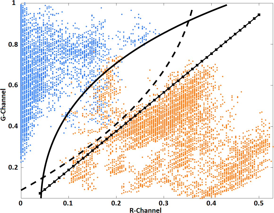
Figure 1: Decision boundaries of SVM #1 (dashed line), SVM #2 (solid line) and $\frac{\rm R}{\rm G}=0.53$ (solid line with dots) for the R(ed) and G(reen) channel training data. Pixels under the SVM #1 boundary are high-confidence lesion seeds, while pixels between the SVM #1 and SVM #2 boundaries are considered to be potential lesion pixels. Orange points denote preselected lesion pixels, and blue pixels are from normal tissue.

To train the boosted decision tree, shallow neural network, and ResNet-101 for informative-frame classification, the training set contained 1000 frames (500 informative, 500 uninformative). Using random selection, 80% of the frames in each class were used to train and the remaining 20% to test. The boosted decision tree was trained in a 5-fold cross-validation procedure. The model with lowest cross-validation loss was used for classification tests, where the model consists of 11 distinct decision trees (220 total decision operations) to boost the result. In concordance with our boosted decision tree’s number of operations, we trained the shallow neural network using 220 hidden neural nodes, with 20% of the training data used to validate the network. With the 7 features (4) serving as the input and ordered as $\alpha,\beta,\ldots\eta$, we arrived at a trained network having derived gains (2.74, 9.11, 2.13, 5.21, 4.73, 0.07, 1.93) and offsets (0.03, 0, 0.06, 0.19, 0.007, 0, 0). Finally, a pre-trained ResNet-101 was retrained as follows [15]: 1) freeze the beginning 10 layers to maintain the feature extractor; 2) replace the last fully connected layer with a new one having only two outputs; 3) use a SGDM (stochastic gradient descent with momentum) optimizer to train the network. Overall, the boosted decision tree, shallow neural network, and ResNet-101 achieved 99%, 90%, and 99.5% correct frame classification in the training data set.

III-B Experimental Results

We tested our methods with the data below:
Case 156 — 4,683-frame HD AFB video having the following ground-truth labels: 4,401 informative frames (93.9% of the total) and 282 noninformative frames (6.1%). Within the informative-frame class, 2,394 were labeled as normal (51.1%) and 2,007 as lesion (42.8%).
Case 157 — 455 HD frames, with each frame randomly selected from a contiguous 10-frame segment of a 4,550-frame sequence. Ground truth: 417, informative; 38, uninformative; all frames normal.
Case 140 — 400-frame SD video sequence consisting entirely of lesion frames.

Regarding Frame Classification, Fig. 2a-b show the 2$\times$2 confusion matrix results produced by the boosted decision tree and ResNet-101. Accuracy results for the methods were as follows. Boosted decision tree — 99.3% and 96.9% for 156 and 157, respectively; ResNet-101 — 97.6% and 95.2%; shallow neural network — 90% and 89%. (Accuracy = (true positives + true negatives) / total frames.) Per the nonnegative gains used for all features (4), the shallow neural network supports the sufficiency of the features used by the boosted decision tree. Fig. 2c shows how the boosted decision tree more robustly detects uninformative frames than ResNet-101 (at least for this sequence and our implementation).

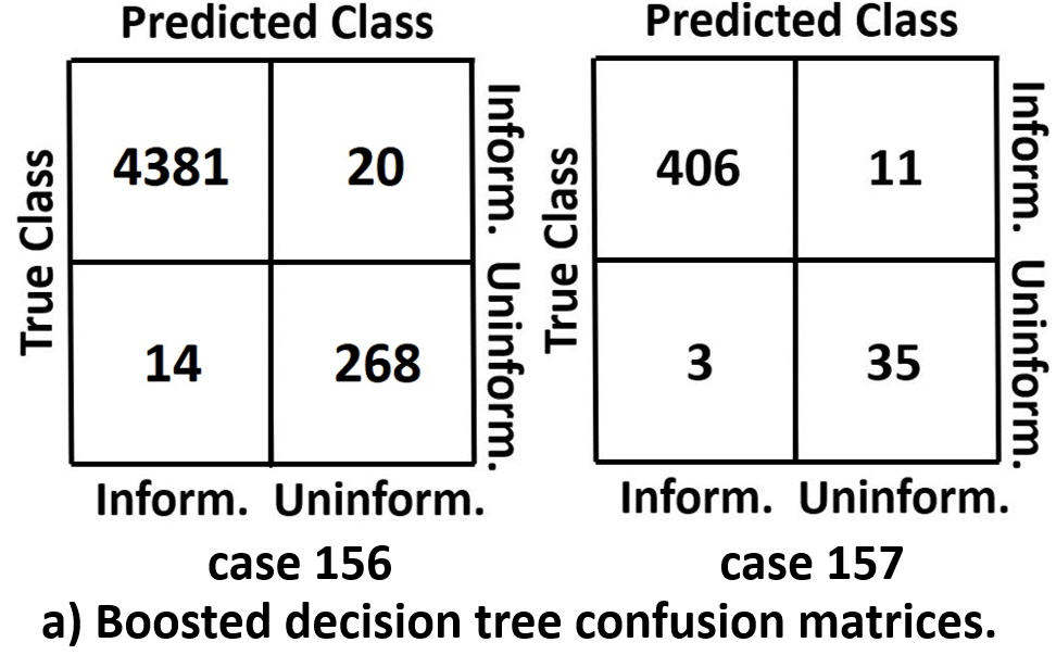
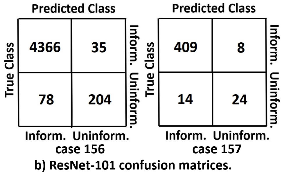
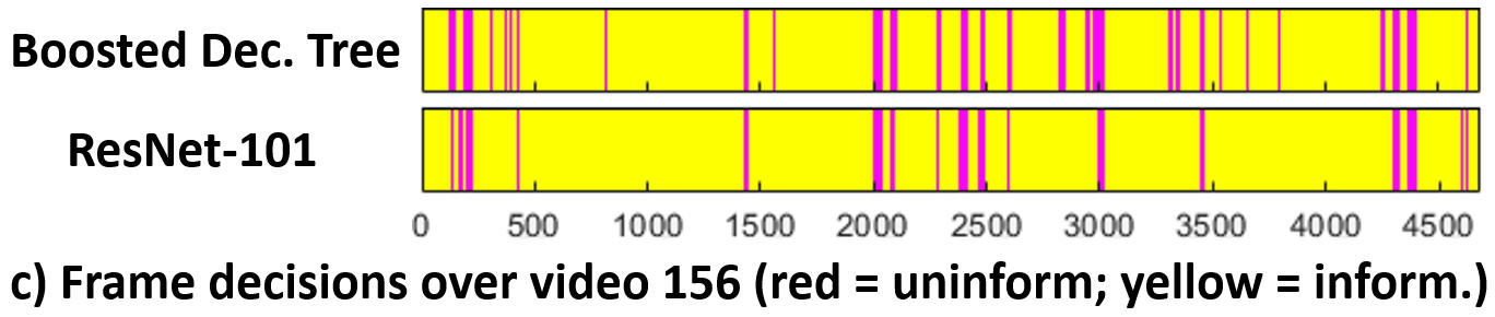
Figure 2: Confusion matrix esults for frame classification. (a) Boosted decision tree. (b) ResNet-101. (c) Method comparison of frame decisions over entire case-156 4,683-frame sequence; yellow = informative frame and red = uninformative frame.

Regarding Lesion Analysis tests, our approach gave the following results for case 156. For lesion frames, 97.1% received correct labels, 2.7% were erroneously labeled normal, and 0.2% were previously classified as uninformative. For normal frames, 97.4% received correct labels, 1.9% received erroneous lesion labels, and 0.7% were previously classified as uninformative. Next, for case 140, 100% of the frames received correct lesion labels (they all also were correctly identified as informative by the boosted decision tree).

As a third test, for a 400-frame sub-segment of case 156 containing only informative frames, Fig. 3 shows the superior performance of our method versus two other methods: the previously suggested Red-to-Green $\frac{\rm R}{\rm G}$ ratio threshold test [16] and another proposal using Fisher’s linear discriminant. A video profile of our method’s class assignments shows that errors tend to be isolated frames (Fig. 4a).  Fig. 4b illustrates a lesion-frame detection. Finally, Fig. 5 shows the superiority of our lesion segmentation method over the $\frac{\rm R}{\rm G}$ method.

	Proposed	Fisher	R/G ratio
Accuracy	98.8%	94.3%	95.0%
sensitivity	99.6%	92.0%	92.8%
specificity	97.1%	98.5%	99.3%

Figure 3: Lesion classification rates for case 156 (400-frame test). Fisher = Fisher’s linear discriminant; R/G ratio = $\frac{\rm R}{\rm G}$ ratio test.

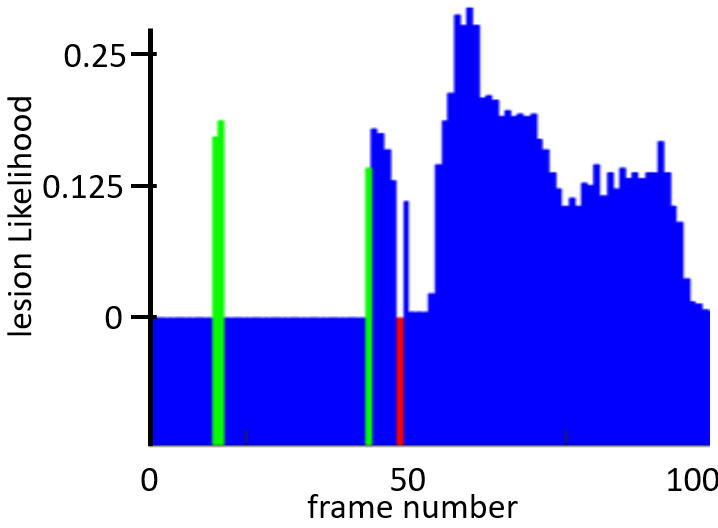
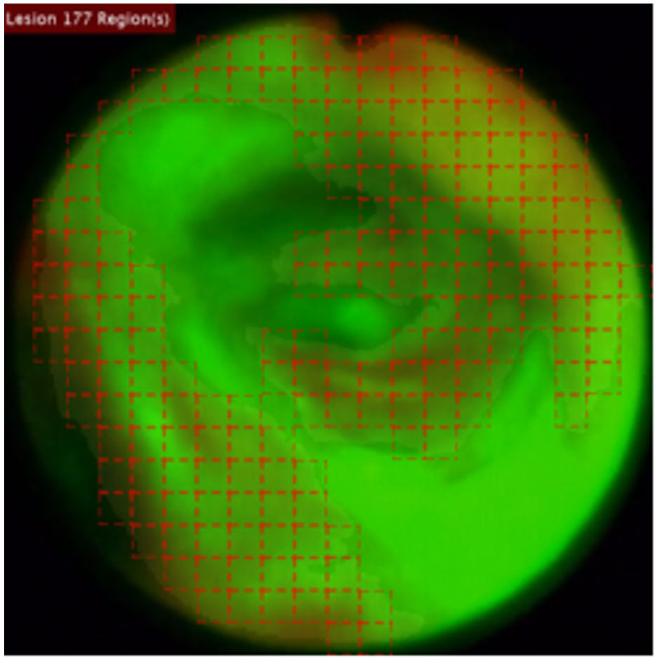
a) Lesion likelihood profile	b) Example lesion frame

Figure 4: Case 156 lesion analysis test. (a) Lesion likelihood profile over a 100-frame segment (blue = correct decision; green = false negative; red = false positive). (b) Flagged lesion frame (lesion likelihood = 0.44); red boxes denote locations of lesion tissue.

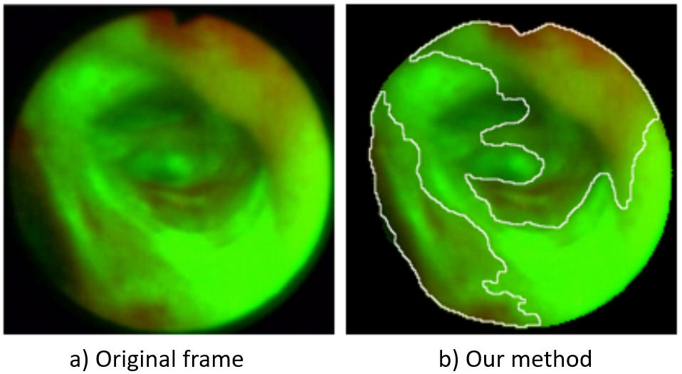
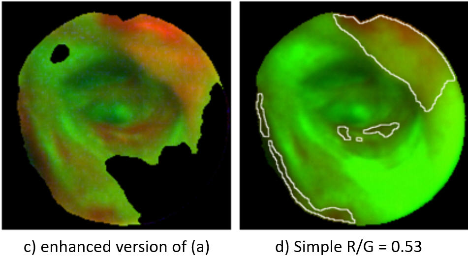
Figure 5: Lesion segmentation example. (a) Original frame. (b) Our method — suspect lesion areas delineated by the white contours. (c) Enhanced version of (a) [8]. (d) $\frac{\rm R}{\rm G}$ ratio test.

IV CONCLUSIONS

We have proposed the first automatic analysis method for AFB video that: 1.) distinguishes uninformative frames from informative frames; and 2.) determines which informative frames contain suspect bronchial lesions and delineates lesion regions. In this way, the search for bronchial lesions becomes more efficient than interactive video browsing and more accurate than simple $\frac{\rm R}{\rm G}$ thresholding. Results show a frame classification accuracy $\geq$97% and a lesion detection accuracy also $\geq$97%. Future work will focus on lesion classification and more extensive tests.

Conflict of Interest: Dr. Higgins and Penn State have financial interests in Broncus Medical, Inc. These financial interests have been reviewed by the University’s Institutional and Individual Conflict of Interest Committees and are currently being managed by the University and reported to the NIH.

References

- [1] F. Bray, J. Ferlay, I. Soerjomataram, R. Siegel, L. Torre, and A. Jemal, “Global cancer statistics 2018: Globocan estimates of incidence and mortality worldwide for 36 cancers in 185 countries,” CA: Cancer J. Clinic., vol. 68, no. 6, pp. 394–424, 2018.
- [2] R. A. van Boerdonk, I. Smesseim, D. A. Heideman et al., “Close surveillance with long-term follow-up of subjects with preinvasive endobronchial lesions,” Am. J. Respir. Crit. Care Med., vol. 192, no. 12, pp. 1483–1489, 15 Dec. 2015.
- [3] E. Billatos, J. Vick, M. Lenburg, and A. Spira, “The airway transcriptome as a biomarker for early lung cancer detection,” Clin. Cancer Res., vol. 24, no. 13, pp. 2984–2992, July 2018.
- [4] J. P. Wisnivesky, R. C.-W. Yung, P. N. Mathur, and J. J. Zulueta, “Diagnosis and treatment of bronchial intraepithelial neoplasia and early lung cancer of the central airways: Diagnosis and management of lung cancer: American college of chest physicians evidence-based clinical practice guidelines,” Chest, vol. 143, no. 5_suppl, pp. e263S–e277S, May 2013.
- [5] T. Inage, T. Nakajima, I. Yoshino, and K. Yasufuku, “Early lung cancer detection,” Clin. Chest Med., vol. 39, pp. 45–55, 2018.
- [6] S. G. Spiro and A. Hackshaw, “Research in progress—LungSEARCH: a randomised controlled trial of surveillance for the early detection of lung cancer in a high-risk group,” Thorax, vol. 71, no. 1, pp. 91–93, 2016.
- [7] P. Byrnes and W. Higgins, “Efficient bronchoscopic video summarization,” IEEE Trans. Biomed. Engin., vol. 66, no. 3, pp. 848–863, March 2019.
- [8] P. Bountris, A. Apostolou, M. Haritou et al., “Combined texture features for improved classification of suspicious areas in autofluorescence bronchoscopy,” in 2009 9th Int. Conf. Inform. Tech. Appl. Biomed., 2009, pp. 1–4.
- [9] X. Zheng, H. Xiong, Y. Li et al., “Application of quantitative autofluorescence bronchoscopy image analysis method in identifying bronchopulmonary cancer,” Tech. Cancer Res. Treat., pp. 1–6, July 2016.
- [10] T. Finkšt, J. F. Tasič, M. Z. Terčelj, and M. Meža, “Classification of malignancy in suspicious lesions using autofluorescence bronchoscopy,” Strojniški vestnik-J. Mech. Engin., vol. 63, no. 12, pp. 685–695, 2017.
- [11] P.-H. Feng, T.-T. Chen, Y.-T. Lin, S.-Y. Chiang, and C.-M. Lo, “Classification of lung cancer subtypes based on autofluorescence bronchoscopic pattern recognition: A preliminary study,” Comp. Meth. Prog. Biomed., vol. 163, pp. 33–38, 2018.
- [12] T. F. Chan and L. A. Vese, “Active contours without edges,” IEEE Trans. Image Proc., vol. 10, no. 2, pp. 266–277, 2001.
- [13] J. Oh, S. Hwang, P. C. de Groen et al., “Informative frame classification for endoscopy video,” Med. Image Analysis, vol. 11, no. 2, pp. 110–127, April 2007.
- [14] M. I. McTaggart and W. E. Higgins, “Robust video-frame classification for bronchoscopy,” in SPIE Medical Imaging 2019: Image-Guided Procedures, Robotic Interventions, and Modeling, vol. 10951, 2019, pp. 109 511Q–1 — 109 511Q–8.
- [15] K. He, X. Zhang, S. Ren, and J. Sun, “Deep residual learning for image recognition,” in Proc. IEEE Conf. Comp. Vision Patt. Recog., 2016, pp. 770–778.
- [16] Y. Kusunoki, F. Imamura, H. Uda, M. Mano, and T. Horai, “Early detection of lung cancer with laser-induced fluorescence endoscopy and spectrofluorometry,” Chest, vol. 118, no. 6, pp. 1776–1782, 2000.