Optimal Delegation in Markets for Matching with Signaling

Abstract

This paper studies a delegation problem faced by the planner who wants to regulate receivers’ reaction choices in markets for matching between receivers and senders with signaling. We provide a noble insight into the planner’s willingness to delegate and the design of optimal (reaction) interval delegation as a solution to the planner’s general mechanism design problem. The relative heterogeneity of receiver types and the productivity of the sender’ signal are crucial in deriving optimal interval delegation in the presence of the trade-off between matching efficiency and signaling costs.

Keywords: competitive signaling equilibrium, full implementation, optimal delegation, stable matching, stronger monotone equilibrium

JEL classification codes: D82, D86

1 Introduction

The design of decision rules by an uninformed principal has been extensively studied in models where she faces an informed but biased agent. (e.g., how a regulator regulate the prices charged by a monopolist whose cost structure is his own private information, how the U.S. House of Representative should regulate the drafting of bills by standing committee, how an organization delegates the choice of decisions to a subordinate, etc.)

Holmstrom (1977, 1984) showed that the problem of finding the optimal decision rule reduces to a delegation problem where the principal simply decides a set of decisions and then the agent is allowed to make any decisions from the delegated set. He characterized optimal delegated sets in various examples. Melumad and Shibano (1991) and Alonzo and Matouschek (2008) provide a full characterization of the optimal delegated sets in more general environments. More recently, the studies of delegation are extended to dynamic setting with a principal and an agent, incorporating learning (Escobar and Zhang (2021), Guo (2016), Lipnowski and Ramos (2020)).

This paper introduces a delegation problem of the planner who wants to regulate receivers’ reaction choices in markets for matching with signaling. In these markets, there is a continuum of heterogeneous senders and receivers (e.g., sellers and buyers, workers and firms, and entrepreneurs and investors) in terms of their types. Each player’s type is their own private information.

For example, prior to entering the job market, workers (senders) often acquire education (action) and it has a signaling effect on their type. Signaling creates a trade-off in matching markets. It increases the efficiency of matching between senders and receivers because separating induces assortative matching. On the other hand, it is costly in that senders need to choose inefficiently high levels of equilibrium actions in order to separate themselves. Because of this trade-off, there may be efficiency gains if the planner regulates receivers’ reaction choices (firms’ wages) to prevent a separating equilibrium from happening in the first place.

Studying the optimal delegation of the planner who wants to maximize equilibrium aggregate net surplus in these markets, we address the following questions. Is there no loss of generality for the planner to focus on intervals of reactions even if she can use any mechanism? When is it better to impose a single reaction to all receivers rather than the full delegation without any restrictions on reactions? When is it optimal for the planner to impose her best single reaction to all receivers instead of delegating reaction choices to receivers? When does the planner provide more discretion to receivers when delegating their reaction choices?

To address these questions, a new methodology is required because those techniques and tools developed in the literature on optimal delegation are largely irrelevant for the analysis of optimal delegation in markets for matching with signaling. The first part of our paper develops a methodology. As in most of the literature on delegation, our model assumes that the planner cannot make transfers to receivers.

In our model, the planner moves first by publicly announcing a mechanism that specifies a receiver’s reaction as a function of his message to her. After observing the mechanism, senders take actions. Given the announced mechanism and the actions taken by senders, one-to-one matching occurs between senders and receivers on the market. As matching take places, a receiver sends a message to the planner and takes the reaction determined by the mechanism given his message.

A key to the mechanism design is the timing of the receiver’s communication. Before entering the market and searching for their potential partners, receivers do not have information on actions chosen by senders on the market. This is why the planner lets receivers send messages to her at the matching stage after they observe the distribution of sender actions, even though the mechanism is announced before senders and receivers enter the market. Given the announced mechanism and the distribution of sender actions, matching and receivers’ communication strategy are a stable matching outcome if there is no pair of a sender and a receiver who are strictly better off by forming a new match with the receiver’s alternative message to the planner for his reaction choice.

In the example of firms (receivers) and workers (senders), a firm’s reaction is wage and a worker’s action is education. Given a mechanism announced by the planner, workers and firms have an expectation on the wage that a worker can receive conditional on an education level chosen by any worker on the market. This expectation is captured in a market reaction function. In equilibrium, it crucially depends on the receiver’s belief on the sender’s type conditional on her action. Given a market reaction function, each worker chooses her education. The receiver’s equilibrium communication strategy and matching confirm the expectation in a competitive signaling equilibrium (CSE).

We first establish the Interval Delegation Principle when utility functions are quasilinear with respect to the receiver’s reaction: Given any CSE that can be induced by a mechanism, there exists a corresponding (closed) interval of reactions such that the same CSE occurs when the planner lets receivers choose their preferred reaction directly from the interval without communication. Therefore, there is no loss of generality for the planner to announce an interval of reactions even if any complex mechanism is possible. In principle, when the planner wants to elicit the receiver’s information through communication, she may need to ask him to report not only his private type but also the whole distribution of sender actions because he observes senders’ actions after entering the market. In this sense, the Interval Delegation Principle makes the planner’s mechanism design problem tractable particularly in a matching market.

For the implementation of an allocation, we adopt the notion of stronger monotone CSE proposed by another paper of ours, Han, Sam, and Shin (HSS, 2023) (See Section 3.2). Borrowed the terminology from the mechanism design literature on implementation, we say that an allocation can be fully implementable in a stronger monotone CSE if there exists an interval of reactions that induces it in all stronger monotone CSEs. HSS (2023) shows that when utility functions are quasilinear, a stronger monotone CSE is unique and well-behaved, given any interval of reaction and hence the full implementation in stronger monotone CSE is possible.

Given a reaction interval, a “well-behaved” equilibrium is characterized by the two threshold sender types. The lower threshold sender type specifies the lowest sender type who enters the market, whereas any sender above the upper threshold sender type pools their actions. Senders between the two threshold types separate themselves. If the two threshold types are the same, it becomes a pooling equilibrium. If the upper threshold type is the supremum of the sender types and greater than the lower threshold type, it becomes a separating equilibrium. If the upper threshold type is less than the supremum of the sender types but greater than the lower threshold type, separating and pooling coexist and the equilibrium is said to be strictly well behaved. In the separating part of the equilibrium, matching is assortative in terms of sender action and receiver type (and hence in terms of sender type and receiver type), whereas in the pooling part, it is random.

While the Interval Delegation Principle makes the mechanism design problem tractable, it does not show how to derive an optimal reaction interval. The aggregate net surplus is a function of the two threshold sender types in a unique stronger monotone CSE. We further show that the planner’s optimal delegation problem - i.e., optimal choice of a reaction interval - comes down to the choice of the two threshold sender types. The reason is that choosing the two threshold sender types ($z_{\ell}$ and $z_{h}$) is equivalent to choosing the lower and upper bounds of an interval of reactions in the sense that we can uniquely retrieve the upper and lower bounds, $t_{\ell}$ and $t_{h}$, of the interval of reactions from any given two threshold sender types. If the two bounds of the interval are the same, then the interval collapses to a singleton $\{t^{\ast}\}$. This is the case where the planner simply imposes a single reaction $t^{\ast}$ to all receivers on the market instead of delegating reaction decisions, inducing a pooling equilibrium. If the upper bound of the interval is sufficiently low but higher than the lower bound, the well-behaved equilibrium have separating and pooling at the same time. As the upper bound increases, the pooling part on the top shrinks. When the upper bound is sufficiently high, the well-behaved equilibrium is separating.

For every sender type $z,$ let $n(z)$ be the type of the receiver that has the same percentile as $z$ has. Given any sender type distribution, $n(\cdot)$ characterizes the receiver type distribution. To solve the optimal delegation problem, we adopt a parametrized model, proposing an approach that approximates the distribution of receiver types by two parameters, which are called “scale” ($k$) and “relative spacing” ($q$) such that $n(z)=kz^{q}$. If $q=0,$ all receivers are homogeneous in terms of their types. The gross match surplus between the receiver type $x$ and the sender type $z$ with action $s$ is given by $v(x,s,z)=Axs^{a}z,$ where $a$ can be interpreted as the productivity parameter of the sender’s action. If $a=0$, the sender’s action only has a pure signaling effect.

We first prove that when the relative spacing parameter ($q$) and the productivity parameter of the sender’s action ($a$) are small, it is more efficient for the planner to impose a single reaction to all receivers, inducing a pooling CSE, instead of fully delegating reaction choices to receivers without restriction on reactions. This results holds regardless of the sender type distribution.

For numerical analysis, we choose various baseline distributions for sender types with the support $[0,3]$, which is generated from the Beta distribution multiplied by 3 with various shape parameters. We provide comparative statics as changing various underlying parameters. In all cases, the lower bound of the optimal reaction interval is $t_{\ell}=0$ so that it is optimal not to exclude anyone in the market.

In Design 1, we choose $k=q=1$ so that both sides of the market have the same type distribution. We change the upper bound of the type support. Regardless of its value, the planner chooses the upper bound of the optimal reaction interval $t_{h}$ in a way that it induces a strictly well-behaved stronger monotone CSE with a pooling part on the top. This suggests that the savings in the cost associated with the pooled action chosen by the sender types above the upper threshold type ($z_{h}$) outweighs the inefficiency associated with random matching in the pooling part. As the upper bound of the type support increases, the planner gives more discretion to receivers in that $t_{h}$ increases in $z_{h}$. While $z_{h}$ also increases in the upper bound of the type support, the percentile of $z_{h}$ is independent of the upper bound of the type support.

In Design 2, we choose $q=1$ given each sender type distribution, changing $k$. As $k$ changes, it changes every receiver type by the same scale. Regardless of the value of $k,$ the planner again chooses $t_{h}$ in a way that it induces a strictly well-behaved CSE with a pooling part on the top. The planner gives more discretion to receivers in that $t_{h}$ increases in $k.$ However, the upper threshold type ($z_{h}$) is independent of $k,$ leaving its percentile constant with respect to $k$ due to the scaling effect associated with $k$. In Design 3, we fix $k=1$ and change $q$ given each sender type distribution. A change in $q$ changes every receiver type by the same factor. As $q$ increases, the planner also increases $t_{h}$ to raise $z_{h}$ in a way that the percentile of $z_{h}$ increases, shrinking the pooling part on the top, due to the spacing effect associated with $q$.

Designs 2 and 3 reflect the empirical findings in Poschke (2018), which show that the mean and variance of the firm size distribution are larger in rich countries and have increased over time for U.S. firms. In our numerical analysis, an increase in $k$ or $q$ each results in increases in both the mean and variance of the receiver type distribution. The results in Designs 2 and 3 show that as the mean and variance of the firm size distribution increase, the planner gives more discretion to receivers. However, she gives a lot more discretion to receivers when increases in the mean and variance of the receiver type distribution come from an increase in $q$ rather than $k$. The reason is that an increase in $q$ increases the percentile of the threshold sender type that starts choosing a pooled action, whereas the percentile is independent of $k$. This makes the solution paths of $t_{h}$ with respect to $q$ more convex since the nonlinear transformation moves a lot more weights on higher types.

In the first three designs, we provide comparative statics given a fixed value for the productivity parameter $a$ of the sender’s action. In Design 4, we change the value of $a$, along with the value of $q.$ Notably, when the sender’s action has only a pure signaling effect ($a=0$) and $q$ is small, it is optimal for the planner to impose her best single reaction to all receivers and induce a pooling CSE, instead of delegating reaction choices to receivers. However, for any given positive value of $a$ and any given $q,$ delegation is better than imposing a single reaction because the optimal stronger monotone CSE is strictly well-behaved. As $a$ increases, both $t_{h}$ and $z_{h}$ increase.

Given type distributions, the utility indifference conditions, (15) and (16), play the crucial role in determining $t_{h}$ (or equivalently $z_{h}$). Since the whole type distributions affect the determination of $t_{h}$ ($z_{h}$) in a non-trivial way through the indifference conditions, we cannot always provide a clear picture about how changes in the underlying type distributions would change the planner’s delegation decision. For example, suppose that both sides of the market have the same type distribution. As we change the type distribution to a first order stochastically dominant one, we may expect that it is optimal for the planner to give discretion to receiver (higher $t_{h}$) to push up $z_{h}$. However we do not have such a monotone relationship (See Table 1).

1.1 Related literature

Delegation problems have been studied in various problems such as tariff caps (Amador and Bagwell (2013)), delegated project choice (Armstrong and Vickers (2010)), consumption-saving problems (Amador, Ivan, Angeletos (2006)), min-max optimal mechanisms (Frankel (2014)), monetary policy (Athey, Atkeson, Kehoe (2005)), veto-based delegation (Mylovanov (2008)), dynamic delegation (Escobar and Zhang (2021), Grenadier, Malenko, and Malenko (2016), Guo (2016), Lipnowski and Ramos (2020)).

Most of works on optimal delegation have focused on a single principal and a single agent. Starting from the seminal paper by Holmstrom (1977, 1984), he asks how a principal should optimally delegate decision-making to an informed, but biased agent. He characterizes optimal delegation sets in various examples mostly with the constraints that only interval delegations are allowed.

Melumad and Shinabo (1991) separately consider (i) the framework in Holmstrom (1977, 1984) where the principal commits to take a decision rule, and (ii) the cheap-talk framework by Crawford and Sobel (1982) where the principal has no commitment power. They characterize the optimal delegation sets without imposing any restrictions on the delegation sets. Their model considers the quadratic loss function in which the preferred decisions are linear functions of the agent’s private type which is uniformly distributed. Alonso and Matouschek (2007) also fully characterize optimal decision-making rule for any commitment power and show conditions under which optimal decision-making rule takes the form of interval delegation and other forms of delegations.

Alonso and Matouschek (2008) extend the model by Melumad and Shinabo (1991) by allowing for general distributions of the agent’s private information and more general utility functions. As assumed in all the above works, in their model, there are no transfers between the principal and the agent. They provide a necessary and sufficient condition for the principal to benefit from delegating decisions to the agent. They further show that when the agent’s preferences are more aligned to the principal’s, interval (threshold) delegation is optimal. Similar to theirs, we also perform comparative statics on the principal’s willingness to delegate decisions to agents, and when interval delegation is optimal. Unlike in Holmstrom (1977, 1984) and most of the follow-up papers, in our work, there is a continuum of agents on both sides of a market.

To our knowledge, our paper is the first that brings a delegation problem to markets for matching with signaling. By doing so, we provide a noble insight into the planner’s willingness to delegate and the optimal delegation.

Our methodology is new. Of course, pre-match investment competition to match with a better partner has been studied in the literature as a potential solution for the hold-up problem of non-contractible pre-match investment that prevails when a match is considered in isolation (e.g. Grossman and Hart (1986) and Williamson (1986)). Cole, Mailath, and Postlewaite (1995), Rege (2008), and Hoppe, Moldovanu, and Sela (2009) consider pre-match investment with incomplete information and non-transferable utility without monetary transfers (i.e., no reaction choice by a receiver). Therefore, the sender-receiver framework does not apply. Pre-match investment with incomplete information in Hopkins (2012) includes the transferable-utility case but with no restrictions on transfers (i.e., no restrictions on reactions). A separating equilibrium is their focus. Furthermore, optimal delegation has never been studied in the models for pre-match investment competition.

While the literature has studied monotone equilibrium, exploring complementarities between actions and types, they mostly focus on games with simultaneous moves and no signaling (Athey (2001), McAdams (2003), Reny and Zamir (2004), Reny (2011), Van Zandt and Vives (2007)). For the optimal delegation in markets for matching with signaling, we adopt the solution concept of a stronger monotone CSE (HSS (2023)), given an reaction interval chosen by the planner. In this equilibrium, a market reaction function, a sender action function, a matching function, and a belief function are all monotone in the stronger set order (Shannon (1995)). Given the uniqueness of a stronger monotone CSE, we show that choosing a reaction interval is equivalent to the two threshold sender types in a unique stronger monotone equilibrium induced by the interval.

Liu and Pei (2020) consider a game with one sender and one receiver where actions, reactions and types are finite. They show that the monotone-supermodular condition of the sender’s utility is sufficient for the monotonicity of the sender’s mixed strategy when the receiver has only two feasible reactions. HSS (2023) shows that the monotone-supermodular condition of the sender’s utility is in fact sufficient for the stronger monotonicity of a pure-strategy equilibrium in a game with one sender and one receiver regardless of the finiteness of actions, reactions, and types. Such a result is important in that most applications with continuous actions, reactions, and types focus on pure-strategy equilibria.

Mensch (2020) follows Athey (2001), McAdams (2003) and Reny (2011) for the existence of a monotone signaling equilibrium in a two-period game with multiple principals. A problem is the potential discontinuity of the belief function associated with a problem with off-path actions. A trick that he employs is that beliefs are perturbed to ensure that all actions are taken with positive probability. Taking the limit as the perturbations vanish yields a perfect Bayesian equilibrium in the original game. One by-product of this approach is that it uniquely pins down a stronger monotone belief. HSS (2023) shows that the stronger monotonicity is equivalent to Criterion D1 (Cho and Kreps (1987) and Banks and Sobel (1987)). The equivalence between the stronger monotonicity of a belief and Criterion D1 is crucial in deriving a unique stronger monotone CSE given any reaction interval even if the interval induces no separating CSE.

2 Preliminaries

There is a continuum of senders and receivers. A planner wants to regulate receivers’ reaction choices. Senders and receivers can be interpreted as sellers and buyers, workers and firms, or entrepreneurs and investors. A planner can be thought of as a government or policy maker. Receivers and senders are all heterogeneous in terms of types. The sender’s type set is $Z=[\underline{z},\overline{z}]\subset\mathbb{R}$ and the receiver’s type set is $X=[\underline{x},\bar{x}]\subset\mathbb{R}.$ The set of feasible reactions for a receiver is $\mathbb{R}_{+}$, whereas the set of feasible actions for a sender is $S=\mathbb{R}_{+}$.

When a sender of type $z$ chooses action $s$ and is matched with a receiver of type $x$ who takes reaction $t,$ the sender’s utility is $u(t,s,z)$ and the receiver’s utility is $g(t,s,z,x)$. The interpretation of types, actions and reactions depend on the examples considered. In the example of firms (receivers) and workers (senders), a sender’s action is education and a receiver’s reaction is wage. We assume the following quasilinear utility functions:

$$u(t,s,z) = t-c(s,z),$$

$$g(t,s,z,x) = v(s,z,x)-t,$$

where $c(s,z)$ is the utility cost incurred to the sender of type $z$ when she choose action $s$ and $v(s,z,x)$ can be thought of as match surplus created between the receiver of type $x$ and the sender of type $z$ with action $s$.

Assume that the measures of senders and receivers are one, respectively. Let $G(z)$ and $H(x)$ denote cumulative distribution functions (CDFs) for sender types and receiver types, respectively. $G$ and $H$ are public information but each individual’s type is their own private information. A sender (receiver) takes zero (re)action $0$ to stay out of the market.

The planner wants to regulate receivers’ reaction choices. It announces a mechanism $\psi:R\rightarrow\mathbb{R}_{+}$ that specifies a receiver’s reaction $t\in\mathbb{R}_{+}$ as a function of his message $r\in R.$ We assume that $range(\psi):=\{\psi(r):r\in R\}$ is closed. Let $\Psi$ be the set of all feasible mechanisms.

The timing unfolds as follows.

1. Senders and receivers observe their own type drawn from $G$ and $H$, respectively.

2. A planner publicly announces a mechanism $\psi:R\rightarrow\mathbb{R}_{+}.$

3. Each sender simultaneously chooses her action.

4. Receivers observe the whole distribution of actions chosen by senders on the market. As one-to-one matching between senders and receivers take places in the market, each receiver sends a message $r$ to a planner. Then, his reaction is determined by $\psi(r)$.

There is no restriction on the message space $R$. The receiver sends a message to the planner at the time of matching. Therefore, a message can be quite complex because a receiver has information not only about his type but also about the distribution of actions chosen by senders in the market.

As described later, one-to-one matching and receivers’ communication with the planner are formulated as a stable bargaining outcome in a cooperative game given a mechanism and senders’ actions. In stable matching, there is no pair of a sender and a receiver who are better off by forming a new match.

3 Full Implementation through Interval Delegation

Let us fix a mechanism $\psi:R\rightarrow\mathbb{R}_{+}$. Let $\sigma(z)$ be the optimal action chosen by a sender of type $z$. Given $\sigma:Z\rightarrow S$, let $range(\sigma):=\{\sigma(z):z\in Z\}$ and $S^{\ast}:=range(\sigma)\backslash\{0\}$. Therefore, $S^{\ast}$ denote the set of actions chosen by senders who enter the market.

Let $co(A)$ be the convex hull of $A$ for some set $A$. When senders make their action choices, they have a belief on the reaction chosen by a receiver whom they can be matched with, conditional on an action $s\in S^{\ast}.$ Receivers also have a belief on the reaction they have to take conditional on the action of the sender whom they are matched with. This belief is captured in a market action function $\tau:S^{\ast}\rightarrow$ $co(range(\psi)).$ A receiver’s communication strategy $\rho:S^{\ast}\times X\rightarrow\Delta(R)$ specifies a probability distribution for his message to the planner conditional on his type $x$ and action $s\in S^{\ast}$ of the sender whom he wants to be matched with. Let $\mathbb{E}_{\rho\left(s,x\right)}\left[\cdot\right]$ be the expectation operator over $R$ given $\rho\left(s,x\right)\in\triangle(R)$.

Definition 1

A receiver’s communication strategy $\rho:S^{\ast}\times X\rightarrow\Delta(R)$ is conformative if

$$\mathbb{E}_{\rho\left(s,x\right)}\left[\psi(r)\right]=\tau(s)\text{ }\forall(s,x)\in S^{\ast}\times X\text{.}$$

Let $\mu:S\rightarrow\Delta(Z)$ characterize receivers’ belief on the sender’s type as a probability distribution conditional on her action. A receiver’s matching problem can be formulated as follows:

$$\max_{s\in S^{\ast}}\;\mathbb{E}_{\mu(s)}\left[v(s,z,x)\right]-\tau(s)\text{ s.t. }\mathbb{E}_{\mu(s)}\left[v(s,z,x)\right]-\tau(s)\geq 0,$$ (1)

where $\mathbb{E}_{\mu(s)}\left[\cdot\right]$ be the expectation operator over $Z$ given $\mu(s)\in\triangle(Z)$.

Let $\xi(x)$ be the action of the sender whom the receiver of type $x$ optimally chooses as his match partner. If (1) has a solution for $x\in X,$ $\xi(x)$ is the solution. Otherwise, $\xi(x)=0.$ Let $X^{\ast}$ denote the set of receiver types such that $\xi(x)$ is a solution for (1). Then, $X^{\ast}$ is the set of receiver types who enter the market.

Consider a sender’s action choice problem. Let $\sigma(z)\in S^{\ast}$ be the optimal action for a sender of type $z$ if (i) it solves the following problem,

$$\max_{s\in S^{\ast}}\;\tau(s)-c(s,z)\text{ s.t. }\tau(s)-c(s,z)\geq 0,$$ (2)

and (ii) there is no profitable sender deviation to an off-path action $s^{\prime}\notin range(\sigma)$ (see Definition 2 below). Note that $\sigma(z)=0$ becomes the optimal action for a sender of type $z$ if there is no solution for (2) and there is no profitable sender deviation to an off-path action $s^{\prime}\notin range(\sigma)$.

Definitions 2, 3, and 4 below define the notions of no profitable sender deviation to an off -path action, stable matching, and competitive signaling equilibrium (CSE), respectively. These definitions are similar to the corresponding ones in HSS (2023) but they incorporate the receiver’s communication strategy with the planner at the time of matching.

For all $s\in S^{\ast},$ let $m(s)\in B(X^{\ast})$ be the set of receiver types who are matched with a sender with $s$, where $B(X^{\ast})$ is the Borel sigma-algebra on $X^{\ast}$ Therefore, $m:S^{\ast}\rightarrow B(X^{\ast})$ is a set-valued matching function. For all $x\in X^{\ast}$, $m^{-1}(x)\in S^{\ast}$ denotes the action chosen by a sender with whom a receiver of type $x$ is matched, i.e., $x\in m\left(m^{-1}(x)\right)$.

Definition 2

Given $\{\sigma,\mu,\tau,m\}$, there is a profitable sender deviation to an off-path action if there exists $z$ for which there are an action $s^{\prime}\notin range(\sigma)$ and a message distribution $\rho^{\prime}\in\triangle(R)$ such that, for some $x^{\prime}$,

(a) $$\mathbb{E}_{\mu(s^{\prime})}\left[v(s^{\prime},z^{\prime},x^{\prime})\right]-\mathbb{E}_{\rho^{\prime}}\left[\psi(r)\right]>\mathbb{E}_{\mu(m^{-1}(x^{\prime}))}\left[v(m^{-1}(x^{\prime}),z^{\prime},x^{\prime})\right]-\tau\left(m^{-1}(x^{\prime})\right)\text{ and }$$ (3)

$$\text{(b) }\begin{array}[]{c}\mathbb{E}_{\rho^{\prime}}\left[\psi(r)\right]-c(s^{\prime},z)>\tau(\sigma(z))-c(\sigma(z),z)\text{ if }\sigma(z)\in S^{\ast},\\ \mathbb{E}_{\rho^{\prime}}\left[\psi(r)\right]-c(s^{\prime},z)>0\text{ otherwise.}\end{array}$$ (6)

Note that $z^{\prime}$ on each side of (3) is the random variable governed by $\mu(s^{\prime})$ and $\mu(m^{-1}(x^{\prime}))$ respectively. If (3) and (6) are not satisfied, there is no profitable sender deviation to an off-path action. The reason is that those are the conditions for sender $z$ to get a higher utility by forming a match with a receiver on the market.Let $B(S^{\ast})$ be the Borel-sigma algebra on $S^{\ast}$.

Definition 3

Given $\{\sigma,\mu\},$ $\{\rho,\tau,m\}$ is a stable matching outcome if

1. $\rho$ is conformative,

2. $\tau$ clears the markets:

   $$H\left(\left\{x|x\in m(\xi(x))\text{, }\xi(x)\in A\right\}\right)=G\left(\left\{z|\sigma\left(z\right)\in A\right\}\right)~{}~{}\forall A\in B(S^{\ast}),$$

3. $m$ is stable: there is no pair of a sender with action $s\in S^{\ast}$ and a receiver of type $x\notin m\left(s\right)$ such that for some $\rho^{\prime}\in\triangle(R)$ and some $z\in$ with $\sigma(z)=s$

   $$\text{(a) }\mathbb{E}_{\mu(s)}\left[v(s,z^{\prime},x)\right]-\mathbb{E}_{\rho^{\prime}}\left[\psi(r)\right] > \mathbb{E}_{\mu(m^{-1}(x))}\left[v(m^{-1}(x^{\prime}),z^{\prime},x)\right]-\tau(s)$$

   $$\text{(b) }\mathbb{E}_{\rho^{\prime}}\left[\psi(r)\right]-c(s,z) > \tau(s)-c(s,z)$$

Definition 3.(iii) implies that the induced $m$ is stable where no two agents would like to block the outcome after every sender has chosen her action in the sense that they form a new match to be better off.

Definition 4

Fix the planner’s mechanism $\psi$. $\{\sigma,\mu,\rho,\tau,m\}$ constitutes a competitive signaling equilibrium (CSE) if

1. for all $z\in Z$, $\sigma(z)$ is optimal

2. $\mu$ is consistent:

   1. if $s\in range(\sigma)$ satisfies $G(\{z|\sigma(z)=s\})>0,$ then $\mu(s)$ is determined from $G$ and $\sigma,$ using Bayes’ rule.

   2. if $s\in range(\sigma)$ but $G(\{z|\sigma(z)=s\})=0$, then $\mu(s)$ is any probability distribution with $supp(\mu(s))=$ cl $\left\{z|\sigma(z)=s\right\}$

   3. if $s\notin range(\sigma)$, then $\mu(s)$ is unrestricted.

3. given $\{\sigma,\mu\},$ $\{\rho,\tau,m\}$ is a stable matching outcome.

3.1 Interval delegation

An interval menu is a special mechanism with the message space is $R=\mathbb{R}_{+}$. Let $T=[t_{\ell},t_{h}]$ be an closed connected interval in $\mathbb{R}_{+}.$ Let $\mathcal{T}$ be a set of all possible closed connected intervals. For some $T\in\mathcal{T}$, let $\overline{\psi}:\mathbb{R}_{+}\rightarrow T$ is called an interval menu if

$$\overline{\psi}(t)=\left\{\begin{array}[]{cc}t&\text{if }t\in T\\ t^{\circ}&\text{otherwise}\end{array}\right.,$$

where $t^{\circ}$ is an arbitrary reaction in $T$. Let $\overline{\Psi}$ be the set of all possible interval menus.

Fix an interval menu $\overline{\psi}:\mathbb{R}_{+}\rightarrow T.$ Given a market reaction function $\tau:S^{\ast}\rightarrow T,$ the receiver’s communication $\rho:S^{\ast}\times X\rightarrow\mathbb{R}_{+}$ is pure conformative if

$$\overline{\rho}(s,x)=\tau(s)~{}~{}\forall(s,x)\in S^{\ast}\times X\text{.}$$

Proposition 1 (Interval Delegation Principle)

Let $\{\sigma,\mu,\rho,\tau,m\}$ be a CSE given a mechanism $\psi:R\rightarrow\mathbb{R}_{+}$ announced by the planner. Then, $\{\sigma,\mu,\overline{\rho},\tau,m\}$ is a CSE given an interval menu $\overline{\psi}:\mathbb{R}_{+}\rightarrow T$ with $T=co($range $\psi)$.

Proof. Given a mechanism $\psi:R\rightarrow\mathbb{R}_{+}$, we have that

$$\left\{\mathbb{E}_{\rho^{\prime}}[\psi(r)]\in\mathbb{R}_{+}:\rho^{\prime}\in\triangle(R)\right\}=co(\text{range }\psi).$$ (7)

Suppose that the planner announces an interval menu $\overline{\psi}:\mathbb{R}_{+}\rightarrow T$ with $T=co($range $\psi)$. Because $\{\sigma,\mu,\rho,\tau,m\}$ is a CSE given $\psi:R\rightarrow\mathbb{R}_{+},$ (7) implies that there is no profitable sender deviation to an off-path action given $\{\sigma,\mu,\tau,m\}$, that is, there is no sender type $z$ for which there are an action $s^{\prime}\notin$ range $\sigma$ and and $t^{\prime}\in T$ such that, for some $x^{\prime}$,

$$\text{{(a)} }\mathbb{E}_{\mu(s^{\prime})}\left[v(s^{\prime},z^{\prime},x^{\prime})\right]-t^{\prime}>\mathbb{E}_{\mu(m^{-1}(x^{\prime}))}\left[v\left(m^{-1}(x^{\prime}),z^{\prime},x^{\prime}\right)\right]-\tau\left(m^{-1}(x^{\prime})\right)\text{, }$$

$$\text{{(b)} }\begin{split}t^{\prime}-c(s^{\prime},z)&>\tau(\sigma(z))-c(\sigma(z),z)\hskip 15.0pt\mbox{ if }\sigma(z)\in S^{\ast}\text{, }\\ t^{\prime}-c(s^{\prime},z)&>0,\hskip 95.0pt\mbox{ otherwise}.\end{split}$$

Furthermore, (7) implies that given $(\sigma,\mu),$ $\{\overline{\rho},\tau,m\}$ is a stable matching outcome because (i) $\overline{\rho}$ is (pure) conformative, (ii) $\tau$ clears the markets, i.e., for all $A\in P(S^{\ast})$ such that $H\left(\left\{x|x\in m(\xi(x))\text{, }\xi(x)\in A\right\}\right)=G\left(\left\{z|\sigma\left(z\right)\in A\right\}\right)$, (iii) $m$ is stable, i.e., there is no pair of a sender with action $s$ and a receiver of type $x\notin m\left(s\right)$ such that, for some $t^{\prime}\in T$ , some $z$ with $\sigma(z)=s\in S^{\ast}$,

(a) $$\mathbb{E}_{\mu(s)}\left[v(s,z^{\prime},x)\right]-t^{\prime}>\mathbb{E}_{\mu(m^{-1}(x))}\left[v(m^{-1}(x),z^{\prime},x)\right]-\tau(s),$$

(b) $$t^{\prime}-c(s,z)>\tau(s)-c(s,z).$$

Therefore, $\{\sigma,\mu,\overline{\rho},\tau,m\}$ is a CSE given an interval menu $\overline{\psi}:\mathbb{R}_{+}\rightarrow T$ with $T=co($range $\psi)$.   

In principle, when the planner wants to elicit the receiver’s information through communication, she may need to ask him to report not only his private type but also the whole distribution of sender actions because he observes senders’ actions after entering the market. In this sense, the Interval Delegation Principle in Proposition 1 makes the planner’s mechanism design problem tractable particularly in matching markets.

From now on, we use an interval $T$ and an interval menu $\overline{\psi}:\mathbb{R}_{+}\rightarrow T$ interchangeably. Further, we drop the pure conformative communication strategy $\overline{\rho}$ when we refer a CSE. $\{\sigma,\mu,\tau,m\}$ is a CSE given an interval $T$ with the understanding that a receiver directly chooses his reaction from $T$ when the planner announces $T\subset\mathcal{T}$. We say that $T$ provides more discretion to receivers than $T^{\prime}$ does if $T\supset T^{\prime}$ and $T\neq T^{\prime}$.

3.2 Full implementation

The allocation is $\{\sigma,\tau,m\}$ given a CSE, $\{\sigma,\mu,\tau,m\}$. Borrowing the terminology from the mechanism design literature on implementation, we say that an allocation $\{\sigma,\tau,m\}$ is fully implemented in stronger monotone CSE if every stronger monotone CSE given some $T\in\mathcal{T}$ induces $\{\sigma,\tau,m\}$.

HSS (2023) formulates a stronger monotone CSE. Consider two sets $A$ and $B$ in the power set $P(Y)$ for $Y$ a lattice with a given relation $\geq$. We say that $A\leq_{c}B$, read “$A$ is completely lower than $B$” in the stronger set order if for every $a\in A$ and $b\in B,$ $a\leq b.$

Definition 5 (Stronger set order)

Given a partially ordered set $K$ with the given relation $\geq$, a set-valued function $M:K\rightarrow P(Y)$ is monotone non-decreasing in the stronger set order if $k^{\prime}\leq k$ implies that $M(k^{\prime})\leq_{c}M(k)$.

Fix a CSE $\{\sigma,\mu,\tau,m\}$ given an interval of reactions $T$ chosen by the planner. $\mu:S\rightarrow\triangle(Z)$ is said to be non-decreasing in the stronger set order if $s^{\prime}<s$ implies supp $\mu(s^{\prime})\leq_{c}$supp $\mu(s)$ for all $s,s^{\prime}\in\mathbb{R}_{+}.$

A (set-valued) matching function $m:S^{\ast}\rightarrow P(X^{\ast})$ is said to be non-decreasing in the stronger set order if $s^{\prime}<s$ implies $m(s^{\prime})\leq_{c}m(s)$ for $s,s^{\prime}\in\mathbb{R}_{+}.$ Note that if $\mu$ is monotone in the stronger set order, then the union of supp $\mu(s^{\prime})$ and supp $\mu(s)$ is either the empty set or a singleton for any $s$ and $s^{\prime}$ such that $s\neq s^{\prime}$. The same property holds for $\sigma,\tau,$and $m$ if they are monotone in the stronger set order.

Definition 6 (Stronger Monotone CSE)

A CSE $\left\{\sigma,\mu,\tau,m\right\}$ is stronger monotone if $\sigma,$ $\mu,\tau,$ and $m$ are non-decreasing in the stronger set order.

A stronger monotone CSE is called well-behaved if it is characterized by two threshold sender types, $z_{\ell}$ and $z_{h}$ such that every sender of type below $z_{\ell}$ stays out of the market, every sender in $[z_{\ell},z_{h})$ differentiates herself with her unique action choice, and all senders in $[z_{h},\overline{z}]$ pool themselves with the same action. If $z_{\ell}<z_{h}=\bar{z},$ then a well-behaved CSE is separating. If $z_{\ell}=z_{h},$ then a well-behaved CSE is pooling. If $z_{\ell}<z_{h}<\bar{z},$ then it is strictly well-behaved with both separating and pooling parts in the equilibrium.

Given technical assumptions, HSS (2023) shows that a stronger monotone CSE $\left\{\sigma,\mu,\tau,m\right\}$ is unique and well-behaved given any interval of reactions $T$ chosen by the planner (Theorems 5, 6, and 7) and that if a well-behaved equilibrium includes a separating part, it is differentiable (Theorem 4). Because a stronger monotone CSE $\left\{\sigma,\mu,\tau,m\right\}$ is unique given any interval of reactions $T$, the planner can fully implement an allocation $\{\sigma,\tau,m\}$ given $T$.

4 Optimal Delegation

This section develops a method for solving the planner’s optimal delegation problem based on the characterization of CSE given any reaction interval in HSS (2023). We start with a stronger monotone separating CSE $\{\tilde{\sigma},\tilde{\mu},\tilde{\tau},\tilde{m}\}$ given an interval of reaction $T=[t_{\ell},t_{h}]\subset\mathbb{R}_{+},$ assuming that $t_{h}$ is sufficiently high. A bilaterally efficient action $\zeta(x,z)$ for type $z$ given $x$ maximizes $v(x,s,z)-c(s,z)$ and we assume that

$$v(\underline{x},\zeta(\underline{x},\underline{z}),z)-c(\zeta(\underline{x},\underline{z}),\underline{z})\geq 0.$$ (8)

We normalize $\zeta(\underline{x},\underline{z})$ to $0.$ Let $z_{\ell}$ be the lowest sender type who is matched in equilibrium and $s_{\ell}$ her action. Then, the following two inequalities must be satisfied at $(s_{\ell},z_{\ell})$:

$$v\left(n\left(z\right),s,z\right)-t_{\ell} \geq 0,$$ (9)

$$t_{\ell}-c\left(s,z\right) \geq 0.$$ (10)

If $z_{\ell}=\underline{z},$ then all types are matched in equilibrium and there is no information rent in the bottom match between type $\underline{z}$ and type $\underline{x}$. Therefore, the equilibrium action $s_{\ell}$ in the lowest match is bilaterally efficient and it is $\zeta(\underline{x},\underline{z})=0$. In this case, we normalize $t_{\ell}=c\left(0,\underline{z}\right)=0$. If $t_{\ell}$ is so high that type $\underline{x}$ cannot achieve a non-negative value of $v-t_{\ell}$ in a match with type $\underline{z}$ who takes an action that costs her $t_{\ell}$, then the lowest match must be between types $z_{\ell}$ and $x_{\ell}:=n(z_{\ell})$ in the interior of both type distributions. (9) and (10) must be satisfied with equality at $(s_{\ell},z_{\ell})$.

We define the function $n$ as $n\equiv H^{-1}\circ G$ so that $H(n(z))=G(z)$ for all $z\in[\underline{z},\overline{z}]$. In a separating equilibrium, matching is assortative and hence the matching function $m$ satisfies $m(s)=n(\mu\left(s\right))$. The first-order conditions for senders and receivers induce the first-order ordinary differential equation for $\mu$:

$$v_{s}(n(\mu(s)),s,\mu(s))+v_{z}(n(\mu(s)),s,\mu(s))\mu^{\prime}(s)-c_{s}(s,\mu(s))=0$$ (11)

with the initial condition $\mu(s_{\ell})=z_{\ell}$.

Once we drive a solution $\tilde{\mu}$, we can construct the functions $\tilde{\sigma},$ $\tilde{\tau},$ and $\tilde{m}$ implied by $\tilde{\mu}$ as follows. $\tilde{\sigma}(z)$ for all $z\in[z_{\ell},\overline{z}]$ is determined by $\tilde{\sigma}(z)=\tilde{\mu}^{-1}(z)$ for all $z\in[z_{\ell},\overline{z}],$ where $\tilde{\mu}^{-1}(z)$ is the type of a sender that satisfies $z=\tilde{\mu}\left(\tilde{\mu}^{-1}(z)\right)$ for all $z\in[z_{\ell},\overline{z}].$ For $s\in[s_{\ell},\tilde{\sigma}(\overline{z})],$ we can derive the matching function $\tilde{m}$ according to $\tilde{m}(s)=n\left(\tilde{\mu}(s)\right)$. The market reaction function $\tilde{\tau}$ becomes

$$\tilde{\tau}(s)=\int_{s_{\ell}}^{s}\left[v_{s}(\tilde{m}(y),y,\tilde{\mu}\left(y\right))+v_{z}(\tilde{m}(y),y,\tilde{\mu}\left(y\right))\tilde{\mu}^{\prime}\left(y\right)\right]dy+t_{\ell}.$$ (12)

If $t_{h}<\tilde{\tau}(\tilde{\sigma}(\bar{z}))$, then we have no separating CSE. In this case, there are two possible stronger monotone equilibria: (i) a stronger monotone pooling CSE and (ii) a strictly well-behaved stronger monotone CSE with $z_{\ell}<z_{h}<\bar{z}$ (i.e., both separating and pooling parts).

If $T$ is a singleton (i.e., $t_{\ell}=t_{h}=t^{\ast}$), a stronger monotone is pooling in the sense that every sender type above $z^{\ast}$ enters the market, choosing a pooled action $s^{\ast}$. The following conditions are satisfied at $(z^{\ast},s^{\ast})$:

$$t^{\ast}-c(s^{\ast},z^{\ast})\geq 0,$$ (13)

$$\mathbb{E}\left[v\left(n\left(z^{\ast}\right),s^{\ast},z^{\prime}\right)|z^{\prime}\geq z^{\ast}\right]-t^{\ast}\geq 0,\text{ }$$ (14)

where each condition holds with equality if $z^{\ast}>\underline{z}.$

A strictly well-behaved stronger monotone CSE with both separating and pooling parts emerges when $t_{\ell}<t_{h}<\tilde{\tau}(\tilde{\sigma}(\bar{z}))$. Any sender type above $z_{h}$ choose the same action $s_{h}.$ The following two equations are satisfied at $(s_{h},z_{h})$ and they are the key to understanding jumping and pooling in the upper tail of the match distributions:

$$t_{h}-c\left(s,z\right)=\tilde{\tau}\left(\tilde{\sigma}\left(z\right)\right)-c\left(\tilde{\sigma}\left(z\right),z\right),$$ (15)

$$\mathbb{E}[v(n\left(z\right),s,z^{\prime})|z^{\prime}\geq z]-t_{h}=v\left(n\left(z\right),\tilde{\sigma}\left(z\right),z\right)-\tilde{\tau}\left(\tilde{\sigma}\left(z\right)\right).$$ (16)

Let $x_{h}:=n(z_{h})$. Theorem 6 in HSS (2023) establishes the existence of a unique well-behaved stronger monotone CSE $\left\{\hat{\sigma},\hat{\mu},\hat{\tau},\hat{m}\right\}$ given $T=[t_{\ell},t_{h}]$ with $0\leq t_{\ell}<\tilde{\tau}(\tilde{\sigma}(\bar{z}))<t_{h}$. It is strictly well behaved.

Figure 1 (borrowed from HSS (2023)) shows the equilibrium sender actions consist of the three different blue parts in a strictly well-behaved stronger monotone CSE $\left\{\hat{\sigma},\hat{\mu},\hat{\tau},\hat{m}\right\}$. Note that equilibrium matching is assortative in terms of sender action and receiver type (and therefore in terms of sender type and receiver type) in the separating part of the CSE but it is random in the pooling part of the CSE. Therefore, there is matching inefficiency in the pooling part but there may be potential savings in the signaling cost associated with the pooled action choice by senders above $z_{h}$.

Theorems 5, 6, and 8 in HSS (2023) establish the unique stronger monotone CSE given each type of the feasible reaction intervals: (i) If $0\leq t_{\ell}<\tilde{\tau}(\tilde{\sigma}(\bar{z}))\leq t_{h}$, then a unique stronger monotone CSE is well-behaved and separating, (ii) If there is only a single feasible reaction, then it is pooling, (iii) If $0\leq t_{\ell}<t_{h}<\tilde{\tau}(\tilde{\sigma}\left(\overline{z}\right)),$ then it is strictly well-behaved with both separating and pooling.

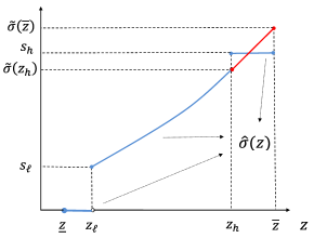
Figure 1: Senders’ equilibrium actions

Lemma 1 shows that the planner only needs to consider a strictly well-behaved stronger monotone CSE because it also covers a stronger monotone separating CSE and a stronger monotone pooling CSE.

Lemma 1

As $z_{h}\rightarrow\bar{z},$ a strictly well-behaved stronger monotone CSE $\left\{\hat{\sigma},\hat{\mu},\hat{\tau},\hat{m}\right\}$ converges to the stronger monotone separating CSE with the same lower threshold sender type $z_{\ell}.$ As $z_{h}\rightarrow z_{\ell},$ $\left\{\hat{\sigma},\hat{\mu},\hat{\tau},\hat{m}\right\}$ converges to the stronger monotone pooling CSE in which $t_{\ell}$ is a single feasible reaction, $z_{\ell}$ is the threshold sender type for market entry, and $s_{\ell}$ is the pooled action for senders in the market.

Combining with Lemma 1, the next two propositions reduce the planner’s optimal delegation problem to the choice of $z_{\ell}$ and $z_{h}$ subject to $z_{\ell}\in Z$ and $z_{h}\geq z_{\ell}$ given that a unique stronger monotone CSE is well-behaved. In other words, for the planner’s optimal delegation, choosing the lower and upper bounds of the feasible reaction interval $T$ is equivalent to choosing the two threshold sender types $z_{\ell}$ and $z_{h}$, one for market entry and the other for pooling on the top.

Proposition 2

(i) For any given $z_{\ell}\in[\underline{z},\overline{z}),$ there exists a unique solution $(s_{\ell},t_{\ell})$ of (9) and (10). (ii) Suppose that the planner chooses $t_{\ell}$ in (i) above Then, $(z_{\ell},s_{\ell})$ solves (9) and (10) given $t_{\ell}$ and it is unique.

Note that if $z_{\ell}=\underline{z}$, then $s_{\ell}=\zeta(\underline{x},\underline{z})=0$. If $z_{\ell}>\underline{z},$ then $s_{\ell}$ is determined uniquely by $z_{\ell}$ because it solves

$$v(n(z_{\ell}),s,z_{\ell})-c(s,z_{\ell})=0,$$ (17)

which is the sum of (9) and (10) with equality. Therefore, Proposition 2 implies that we can retrieve $t_{\ell}$ that induces $(s_{\ell},z_{\ell})$ from (9) with equality when $z_{\ell}=\underline{z}$, or either (9) or (10), each with equality when $z_{\ell}>\underline{z}$. Therefore, the planner’s point of view, choosing $z_{\ell}$ is equivalent to choosing $t_{\ell}$.

Proposition 3

(i) For any given $z_{h}\in(z_{\ell},\overline{z}),$ there exists a unique $(s_{h},t_{h})$ of (15) and (16). (ii) Suppose that the planner chooses $t_{h}$ in (i) above. Then, $(z_{h},s_{h})$ solves (15) and (16) given $t_{h}$ and it is unique.

Note that $s_{h}$ is determined solely by $z_{h}$ because it solves

$$\mathbb{E}[v(n\left(z_{h}\right),s,z^{\prime})|z^{\prime}\geq z_{h}]-c\left(s,z_{h}\right)=v\left(n\left(z_{h}\right),\tilde{\sigma}\left(z_{h}\right),z_{h}\right)-c\left(\tilde{\sigma}\left(z_{h}\right),z_{h}\right),$$ (18)

which is the sum of (15) and (16) at $z_{h}$. Therefore, Proposition 3 implies that we can retrieve $t_{h}$ that induces $(s_{h},z_{h})$ from either (15) or (16). The planner can first choose the threshold sender type $z_{h}$ and retrieve the upper bound of feasible reactions $t_{h}$ that induces $z_{h}$ in a well-behaved equilibrium.

Given a well-behaved stronger monotone CSE $\left\{\hat{\sigma},\hat{\mu},\hat{\tau},\hat{m}\right\}$ with the lower and upper threshold sender types, $z_{\ell}$ and $z_{h}$, the aggregate net surplus is

$$\Pi(z_{\ell},z_{h}):=\int_{z_{\ell}}^{z_{h}}v(n(z),\hat{\sigma}(z),z)dG\left(z\right)-\int_{z_{\ell}}^{z_{h}}c(\hat{\sigma}(z),z)dG\left(z\right)\\ +\int_{z_{h}}^{\bar{z}}\mathbb{E}\left[v(n(z),s_{h}(z_{h}),z^{\prime})|z^{\prime}\geq z_{h}\right]dG\left(z\right)-\int_{z_{h}}^{\bar{z}}c(s_{h}(z_{h}),z)dG\left(z\right),$$

where $s_{h}(z_{h})$ is the pooled action chosen by all sender types above $z_{h}$ and it is unique given any $z_{h}\in[z_{\ell},\bar{z}]$ because of Proposition 3(i). Note that the first line in $\Pi(z_{\ell},z_{h})$ is the aggregate net surplus in the separating part of the equilibrium where matching is assortative in terms of types. The second line is the aggregate net surplus in the pooling part of the equilibrium with random matching and hence matching efficiency is lower in this pooling part but there is potential savings in the cost due to the pooled action chosen by all senders above $z_{h}$.

Theorem 1

Suppose that the planner wants to maximize the aggregate net surplus. The solution for the planner’s optimal delegation problem is the same as the solution for the planner’s design following problem of the optimal stronger monotone equilibrium:

$$\max_{\overline{z}>z_{\ell}\geq\underline{z},z_{h}\geq z_{\ell}}\Pi(z_{\ell},z_{h})$$

If $z_{\ell}<z_{h}<\bar{z},$ then the stronger monotone equilibrium is strictly well-behaved. If $z_{\ell}<z_{h}=\bar{z},$ it is separating. If $z_{\ell}=z_{h}<\bar{z},$ it is pooling.

If $z_{\ell}=z_{h}<\bar{z}$, then the planner simply imposes her best uninformed reaction choice $t^{\ast}$ to all receivers, inducing a pooling equilibrium. When is imposing a single reaction to all receivers better than the full delegation ($T=\mathbb{R}_{+}$)? When is it optimal for the planner to simply impose her best single reaction to all receivers instead of delegating the reaction choice to receivers? Putting it differently, when does the planner benefit from delegation? When does the planner provide a more discretion to receivers when delegating their reaction choices? We address these questions in a parametrized model.

4.1 Parametrized optimal delegation problem

Generally, the aggregate equilibrium surplus depends on $v,$ $c,$ $G$, and $H.$ For the optimal equilibrium design, we propose an approach that approximates the distribution of receiver types with the “shift” and “relative spacing” parameters given an arbitrary distribution of sender types. Consider a gross match surplus function that follows the form of $v(x,s,z)=As^{a}xz$ with $0\leq a<1.$ The cost of choosing an action $s$ is $c(s,z)=\beta\frac{s^{2}}{z}$ for the sender of type $z,$ where $\beta>0$. The lowest sender type is $\underline{z}=0.$

A sender’s type follows a probability distribution $G$, whereas a receiver’s type follows $H$. Recall that $n$ is defined as $H^{-1}\circ G$ so that $H(n(z))=G(z)$ for all $z.$ We assume that $n$ takes the following form:

$$n(z)=kz^{q},$$ (19)

where $k>0$ and $q\geq 0.$ Note that $k$ is the “scale” parameter and $q$ is the “relative spacing” parameter. The relative spacing parameter $q$ shows the relative heterogeneity of receiver types to sender types. Recall that $n(z)$ denotes the type of a receiver who is matched with the sender of type $z$ in the stronger monotone separating equilibrium. This approach is general in the sense that it approximates the distribution of receiver types with the “scale” and “relative spacing” parameters for any arbitrary distribution of sender types.

To derive a well-behaved stronger monotone equilibrium, we first need to solve the first-order differential equation (11) for $\mu$ with the initial condition $(z_{\ell},s_{\ell}).$ The value of $s_{\ell}$ only depends on $z_{\ell}.$ If $z_{\ell}=0,$ then $s_{\ell}(z_{\ell})=\zeta(0,0)=0.$ If $z_{\ell}>0,$ then $s_{\ell}(z_{\ell})$ is determined by (17) and it is $s_{\ell}(z_{\ell})=\left(\frac{Ak}{\beta}z_{\ell}^{q+2}\right)^{\frac{1}{2-a}}$. Note that $s_{\ell}(z_{\ell})$ is continuous everywhere including at $z_{\ell}=0.$

Proposition 4

Given any initial condition $(z_{\ell},s_{\ell}\left(z_{\ell}\right)),$ the solution for first-order differential equation $\mu^{\prime}(s)=\phi(s,\mu(s))$ is

$$\tilde{\mu}(s)=\left[\begin{array}[]{c}\left(\dfrac{2\beta(2+q)}{Ak}\right)\dfrac{s^{2-a}}{2+a+aq}\\ +\left(\dfrac{s_{\ell}(z_{\ell})}{s}\right)^{a(2+q)}\dfrac{\left[Ak(2+a+aq)z_{\ell}^{2+q}-2\beta(2+q)s_{\ell}(z_{\ell})^{(2-a)}\right]}{Ak(2+a+aq)}\end{array}\right]^{\dfrac{1}{2+q}}.$$

Note that $\tilde{\sigma}(z)$ is the inverse of $\tilde{\mu}(s)$, which is derived numerically as $\tilde{\mu}(s)$ does not allow for a closed-form solution for its inverse. Given $z_{h},$ $s_{h}(z_{h})$ is unique and it solves (18), which is

$$Aks_{h}^{a}z_{h}^{q}\mathbb{E}[z^{\prime}|z^{\prime}\geq z_{h}]-\beta\frac{s_{h}^{2}}{z_{h}}=Ak\tilde{\sigma}\left(z_{h}\right)^{a}z_{h}^{1+q}-\beta\frac{\tilde{\sigma}\left(z_{h}\right)^{2}}{z_{h}}.$$ (20)

We need to numerically derive $s_{h}(z_{h})$ as it does not allow for a closed form solution. Given a choice of $z_{\ell}$ and $z_{h}$, the aggregate net surplus is

$$\Pi_{w}(z_{\ell},z_{h},q,a,G)=\int_{z_{\ell}}^{z_{h}}\left[v(n(z),\hat{\sigma}(z),z)-c(\hat{\sigma}(z),z)\right]g(z)dz\\ +\int_{z_{h}}^{\bar{z}}\left[\mathbb{E}[v(n\left(z\right),s_{h}\left(z_{h}\right),z^{\prime})|z^{\prime}\geq z_{h}]-c(s_{h}\left(z_{h}\right),z)\right]g(z)dz\\ =\int_{z_{\ell}}^{z_{h}}\left(Akz^{q+1}\hat{\sigma}(z)^{a}-\beta\frac{\hat{\sigma}(z)^{2}}{z}\right)g(z)dz\\ +Aks_{h}(z_{h})^{a}\mathbb{E}[z^{\prime}|z^{\prime}\geq z_{h}]\int_{z_{h}}^{\bar{z}}z^{q}g(z)dz-\beta s_{h}(z_{h})^{2}\int_{z_{h}}^{\bar{z}}\frac{1}{z}g(z)dz,$$

where $\hat{\sigma}(z)=\tilde{\sigma}\left(z\right)$ for $z\in[z_{\ell},z_{h}].$

Given $(a,q,G),$ we can find the best well-behaved equilibrium through the following maximization problem:

$$\max_{(z_{\ell},z_{h})}\Pi_{w}(z_{\ell},z_{h},q,a,G)$$

$$\text{subject to }0\leq z_{\ell}\leq z_{h}\leq\bar{z}.$$

4.2 More efficient non-separating equilibria

Suppose that the planner fixes the lower bound of feasible reactions such that $z_{\ell}=0$ and hence $s_{\ell}(z_{\ell})=0$ (no sender stays out of the market). In this case, the belief function $\tilde{\mu}(s)$ allows for the closed-form expression of its inverse, which is the sender’s equilibrium action function in the separating equilibrium:

$$\tilde{\sigma}(z)=\left(\frac{Ak}{2\beta}\frac{aq+a+2}{q+2}\right)^{\frac{1}{2-a}}z^{\frac{q+2}{2-a}}\text{ for }z<z_{h}.$$

The aggregate net surplus in the well-behaved stronger monotone equilibrium is

$$\Pi_{w}(0,z_{h},q,a,G)=\\ \left(\left(Ak\right)^{\frac{2}{2-a}}\left(\frac{aq+a+2}{2\beta\left(q+2\right)}\right)^{\frac{a}{2-a}}-\beta\left(\frac{Ak}{2\beta}\frac{aq+a+2}{q+2}\right)^{\frac{2}{2-a}}\right)\int_{0}^{z_{h}}z^{\frac{2q+2+a}{2-a}}dG(z)\\ +Aks(z_{h})^{a}\mathbb{E}[z|z\geq z_{h}]\int_{z_{h}}^{\bar{z}}z^{q}g(z)dz-\beta s_{h}(z_{h})^{2}\int_{z_{h}}^{\bar{z}}\frac{1}{z}g(z)dz.$$

As $z_{h}$ approaches $\bar{z}$, the maximum of the support of $G,$ $\Pi_{w}(0,z_{h},q,a,G)$ becomes the aggregate net surplus $\Pi_{s}(a,q,G)=$ $\Pi_{w}(0,\bar{z},q,a,G)$ without any restrictions on feasible reactions (i.e., $\Pi_{s}(a,q,G)$ is the aggregate net surplus in the baseline separating equilibrium). We show that, when the relative heterogeneity of receiver types ($q$) and the productivity of the sender action ($a$) are not too large, there is an interval of reactions that induces a strictly well-behaved equilibrium that is more efficient than the separating equilibrium with the full delegation (i.e., $T=\mathbb{R}_{+}$) regardless of $G.$

Theorem 2

There are $\hat{q},\hat{a}>0$ such that for any given $(q,a)\in[0,\hat{q}]\times[0,\hat{a}]$, we have an interval of feasible reactions $[0,\hat{t}]$ that induces a unique strictly well-behaved stronger monotone equilibrium, which is more efficient than the stronger monotone separating equilibrium with the full delegation. Given $[0,\hat{t}]$, it is a unique stronger monotone equilibrium.

Proof. First, we construct a (unique) strictly well-behaved stronger monotone equilibrium with $0=z_{\ell}<z_{h}<$ supremum of the support of $G.$ Let $s_{h}(z_{h},a,q)$ be the value of $s_{h}$ that solves (20) at every $a$ and $q.$ Because functions in (20) are continuous in $a$ and $q$, $s_{h}(z_{h},a,q)$ is continuous in $a$ and $q.$ Given (20), we have

$$\lim_{q,a\rightarrow 0}\left(As_{h}(z_{h},q,a)^{a}kz_{h}{}^{q}\mathbb{E}\left[z|z\geq z_{h}\right]-\beta\frac{s_{h}(z_{h},q,a)^{2}}{z_{h}}\right)\\ =\lim_{q,a\rightarrow 0}\left(Ak\tilde{\sigma}\left(z_{h}\right)^{a}z_{h}{}^{q+1}-\beta\frac{\tilde{\sigma}\left(z_{h}\right)^{2}}{z_{h}}\right).$$

Therefore, we have that $\lim_{q,a\rightarrow 0}s_{h}(z_{h},q,a)=\sqrt{z_{h}{}^{2}Ak\left(\mathbb{E}\left[z|z\geq z_{h}\right]-1\right)/\beta}.$ This implies that

$$\lim_{q,a\rightarrow 0}\Pi_{w}(0,z_{h},q,a,G)=\int_{0}^{z_{h}}\frac{Akz}{2}dG(z)+\int_{z_{h}}^{\bar{z}}Ak\mathbb{E}\left[z|z\geq z_{h}\right]dG(z)\\ -z_{h}{}^{2}Ak\left(\mathbb{E}\left[z|z\geq z_{h}\right]-1\right)\int_{z_{h}}^{\bar{z}}\frac{1}{z}dG(z).$$

Taking the limit of $\lim_{q,a\rightarrow 0}\Pi_{w}(0,z_{h},q,a,G)$ with respect to $z_{h}$ yields

$$\lim_{z_{h}\rightarrow 0}\left[\lim_{q,a\rightarrow 0}\Pi_{w}(0,z_{h},q,a,G)\right]=\int_{0}^{\bar{z}}AkzdG(z)=Ak\mu_{z},$$

where $\mu_{z}$ is the unconditional mean of the sender type $z.$

On the other hand, the limit of the aggregate net surplus in the stronger monotone separating equilibrium is

$$\lim_{q,a\rightarrow 0}\Pi_{s}(q,a,G)=\int_{0}^{\bar{z}}AkzdG(z)-\int_{0}^{\bar{z}}\frac{Akz}{2}dG(z)=\frac{Ak\mu_{z}}{2}.$$

Therefore, we have that

$$\lim_{z_{h}\rightarrow 0}\left[\lim_{q,a\rightarrow 0}\Pi_{w}(0,z_{h},q,a,G)\right]-\lim_{q,a\rightarrow 0}\Pi_{s}(q,a,G)=\frac{Ak\mu_{z}}{2}>0.$$ (21)

Because $\Pi_{w}(0,z_{h},q,a,G)$ and $\Pi_{s}(q,a,G)$ are continuous, there exists $\hat{q}>0$, and $\hat{a}>0$ and $\hat{z}_{h}(\hat{q},\hat{a})\in$ Int $Z$ such that for every $(q,a)\in[0,\hat{q}]\times[0,\hat{a}]$ and every $z_{h}\in(0,\hat{z}_{h}(\hat{q},\hat{a})]$, $\Pi_{w}(0,z_{h},q,a,G)>\Pi_{s}(q,a,G)$. We can retrieve $t_{h}$ given $z_{h}\in(0,\hat{z}_{h}(\hat{q},\hat{a})]$. $\blacksquare$

In the well-behaved stronger monotone equilibrium constructed above, a small fraction of senders and receivers on the low end of the type distribution follow their equilibrium sender actions, reactions, and assortative matching that would have occurred in the stronger monotone separating equilibrium. The rest of senders and receivers are matched randomly because the rest of senders all choose the same action. We can also establish that when $a$ and $q$ are small, no delegation is better than the full delegation.

Theorem 3

There are $\tilde{q},\tilde{a}>0$ such that, for any given $(q,a)\in[0,\tilde{q}]\times[0,\tilde{a}]$, we have $t^{\ast}>0$ such that it induces a unique stronger monotone pooling equilibrium that is more efficient than the stronger monotone separating equilibrium with the full delegation.

The intuition behind Theorem 3 is the same as that behind Theorem 2. A major difference is that a pooling equilibrium forces a small fraction of senders and receivers on the low end of type distribution to stay out of the market even though they can produce positive net surplus, whereas everyone is matched in the strictly well-behaved equilibrium identified in Theorem 2. Theorems 2 and 3 in fact show that a separating equilibrium with the full delegation is not optimal in the classical Spencian model (Spence 1973) of pure signaling with no heterogeneity of receivers (i.e., $a=q=0$).

5 Numerical analysis

We turn our attention to numerical analysis. For the concreteness of our numerical analysis, one can think of senders as workers and receivers as firms. A sender’s type can be then viewed as unobservable skill and her action as observable skill. A firm’s type can be viewed as its size. In the literature of empirical macro/development economics, firm size is measured by the amount of labour it employees; In finance, it is measured by the firm’s market value if it is publicly traded. In an entry-level job market, a worker’s unobservable skill could be her ability to understand a task given to her and to figure out how to complete it. In a managerial job market, a worker’s unobservable skill could be her ability to come up with new business idea or innovation.

For numerical analysis, we consider a specific distribution of $G$ with various combinations of underlying parameters. The support of the sender’s type $z$ is set to be $[0,3]$ in the baseline design and is generated from the Beta distribution multiplied by 3 with the following shape parameters: $\{(1,1),(5,5),(3,5),(5,3)\}.$ Figure 2 shows the probability density functions with different shape parameter values. Note that Beta(1,1) corresponds to the uniform distribution and Beta(5,5) to a symmetric bell-shaped distribution. Beta(3,5) and Beta(5,3) correspond to right-skewed and left skewed sender type distributions, respectively. We set the effective zero as $10^{-6}$.

Figure 2: Probability Density Functions of the Beta Distribution

Beta(1,1)	Beta(5,5)	Beta(3,5)	Beta(5,3)

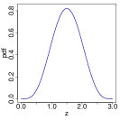
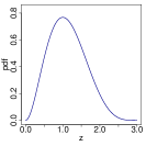
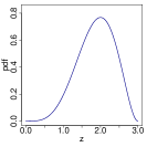
• Notes. The send type variable $z$ is generated by $3\cdot Beta(\cdot,\cdot).$

Figure 3: Design 1. Support Change with Symmetric Distributions

Beta(1,1)
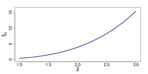
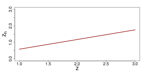
Beta(3,5)
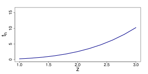
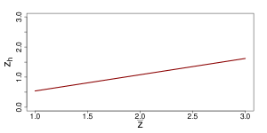
Beta(5,5)
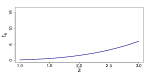
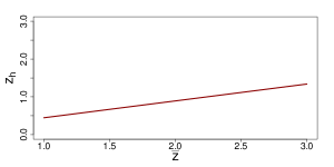
Beta(5,3)

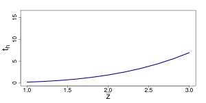
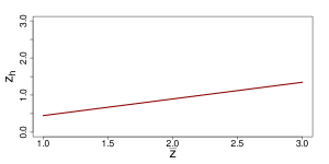
• Notes. This design imposes the same distribution on senders and receivers. We change the upper bound of their supports ($\bar{z}=\bar{x}$). The lower bound of an interval delegation is always zero ($t_{l}=0$). The lower bound of a well-behaved equilibrium is also zero ($z_{l}=0$).

Figure 4: Design 2. Receiver Distribution Change by $k$

Beta(1,1)
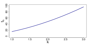
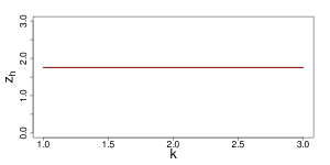
Beta(3,5)
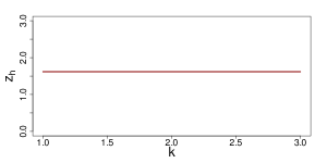
Beta(5,5)
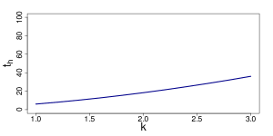
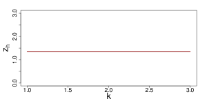
Beta(5,3)

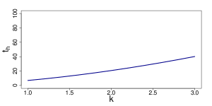
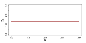
• Notes. This design varies the distribution of the receiver type ($x$) by changing $k$. Recall the matching function $x=kz^{q}$. We keep the same distribution on senders’ type. The lower bound of an interval delegation is always zero ($t_{l}=0$). The lower bound of a well-behaved equilibrium is also zero ($z_{l}=0$).

Figure 5: Design 3. Receiver Distribution Change by $q$

Beta(1,1)
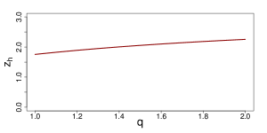
Beta(3,5)
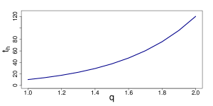
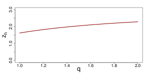
Beta(5,5)
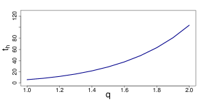
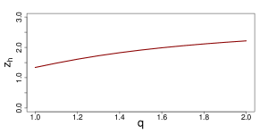
Beta(5,3)

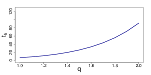
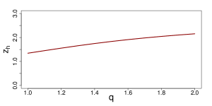
• Notes. This design varies the distribution of the receiver type ($x$) by changing $q$. Recall the matching function $x=kz^{q}$. We keep the same distribution on senders’ type. The lower bound of an interval delegation is always zero ($t_{l}=0$). The lower bound of a well-behaved equilibrium is also zero ($z_{l}=0$).

Figure 6: Design 4. Signal Contribution ($a$) and Receiver Type ($q$)

Beta(1,1)
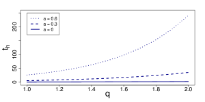
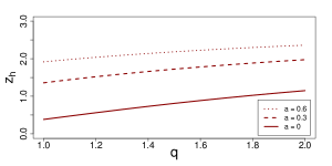
Beta(3,5)
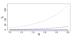
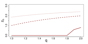
Beta(5,5)
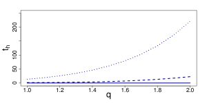
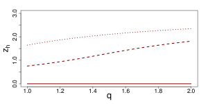
Beta(5,3)

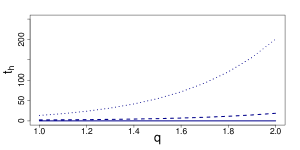
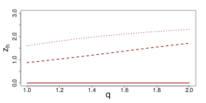
• Notes. This design varies both the signal contribution parameter $a$ and the distribution of the receiver type by $q$. Recall the matching function $x=kz^{q}$ and the match surplus function $v(x,s,z)=As^{a}xz$. We keep the same distribution on senders’ type. The lower bound of an interval delegation is always zero ($t_{l}=0$). The lower bound of a well-behaved equilibrium is also zero ($z_{l}=0$). Graphs with $a=0.9$ are relegated to the appendix because of the scale difference.

Other parameters in the baseline design are set as follows: $A=1,$ $\beta=0.5,$ $a=0.5,$ $k=1$ and $q=1.$ Note that, given $k=q=1,$ we have that $n(z)=x$ in (19). In each design, we depart from the baseline design by changing some parameter values above. In Design 1, senders and receivers have the same type distribution (i.e. a symmetric structure) by keeping $k=1$ and $q=1$. However, we change the support of type distributions. Specifically, we vary the upper bound of the support between 1 and 3. Recall that the upper bound of the baseline design is 3. Then, we check the optimal reaction interval and the corresponding stronger monotone equilibrium. In Design 2, we set the sender type distribution back to the baseline design, i.e. $z\in[0,3]$ and change the scale parameter $k$. Design 3 varies only the relative spacing parameter $q$ while holding all other conditions of the baseline design. Finally, Design 4 varies the signal contribution parameter $a$ as well as the relative spacing parameter $q$.

Due to Theorem 1, we can first derive the optimal $z_{\ell}$ and $z_{h}$ given the type distributions and other parameter values. This determines the type of the optimal stronger monotone CSE. We can then retrieve the corresponding $t_{\ell}$ and $t_{h},$ the lower and upper bounds of the optimal delegation interval. In all cases, $z_{\ell}$ turns out zero so that it is optimal not to exclude anyone in the market and hence $t_{\ell}=0.$ Therefore, we report only the optimal solution paths for $t_{h}$ and $z_{h}$ in Figures 3–6. We also report the solution paths for other variables ($x_{h}$ and $s_{h}$) as well as the support bounds ($\bar{x}$ and $\bar{z}$) in Tables 2–17 that are relegated to the appendix.

Design 1 restricts our attention to the symmetric structure between the sender type and the receiver type, changing only the upper bound of the type distribution support ($\bar{z}=\overline{x}$). Regardless of the value of $\bar{z},$ $z_{h}$ is less than $\overline{z}$ and greater than $z_{\ell}=0.$ Therefore, the optimal stronger monotone CSE is strictly well behaved so that it includes a pooling part on the top. This suggests that the savings in the cost associated with the pooled action chosen by sender types above $z_{h}$ outweighs the inefficiency associated with random matching in the pooling part. As we increase the type distribution support from $[0,1]$ to $[0,3]$, Figure 3 shows that both $t_{h}$ and $z_{h}$ increase monotonically. Therefore, as the upper bound of the type distribution support increases, the planner gives more discretion to receivers with a higher upper bound of the delegation interval, increasing the threshold sender type for pooling. Note that $z_{h}$ has a linear relationship with $\bar{z}$ while $t_{h}$ increases exponentially In fact, the percentile of the threshold sender type $z_{h}$ that starts choosing the pooled action does not change even though $z_{h}$ itself increases as the upper bound of type distribution changes. These results hold across different Beta distributions.

Design 2 departs from the symmetric design by changing the scale parameter $k\in[1,3]$ in $n(z)=kz^{q}$. All other parameters are set to the baseline values. As $k$ increases from 1, it increases every receiver type $x$ by the same scale. Regardless of the value of $k$, the optimal stronger monotone CSE is again strictly well behaved. Note that $z_{h}$ does not vary over different $k$ values. Because the sender type distribution is fixed, this implies that the percentile of $z_{h}$ does not change (See the second column in Figure 4). This makes sense because $k$ has only the scaling effect on the receiver type. However, $t_{h}$ increases in $k$ as the threshold receiver type $\bar{x}$ for pooling increases in $k$ (See the first column in Figure 4). Therefore, we confirm that the planner gives more discretion to receivers when the support of firms gets larger though the scale parameter.

In Design 3, we fix $k=1$ and increase the value of $q$ from 1. Because the initial support of the receiver type is $[0,3]$, the whole distribution of receiver types changes in a way that the receiver type in $[0,1]$ decreases and the receiver type in $[1,3]$ increases by the same factor as $q$ increases. This change results in an increase in $z_{h}$. Since the sender type distribution is fixed in each case, it implies that the percentile of $z_{h}$ increases as $q$ increases. This seems to suggest that the spreading effect on the receiver type in $[1,3]$ of the initial distribution dominates the shrinking effect on the receiver type in $[0,1]$. Subsequently, the planner gives more discretion to receivers by increasing $t_{h}$.

A change in $k$ or a change in $q$ each results in an increase in $t_{h}.$ However, the percentile of $z_{h}$ remains the same with a change in $k$, whereas it increases in $q$. Therefore, an increase in $t_{h}$ should be sufficiently high to satisfy the utility indifference conditions, (15) and (16), at a higher percentile of the threshold type for pooling when $q$ increases. Figure 5 shows that both $t_{h}$ and $z_{h}$ increase monotonically as $q$ increases. However, the solution paths of $t_{h}$ become more convex since the nonlinear transformation moves more weights on higher types.

Designs 2 and 3 also reflect the empirical findings in Poschke (2018) such that the mean and variance of the firm size distribution ($x$) are larger in rich countries and have increased over time for U.S. firms, where the firm size is measured by the number of workers employed. In fact, an increase in $k$ or $q$ each results in increases in both the mean and variance of the receiver type distribution. The results in Designs 2 and 3 show that as the mean and variance of the firm size distribution increase, the planner gives more discretion to receivers. However, when increases in the mean and variance of the receiver type distribution come from an increase in $q$ rather than $k$, the planner gives a lot more discretion to receivers due to more convex solution paths of $t_{h}$ with respect to $q$.

The first three designs provide comparative statics as the underlying type distributions change given a positive value of the productivity paramter of the sender’s action ($a=0.5$). In Design 4, we change the value of $a$ along with $q$. We vary $a\in\{0,0.3,0.6,0.9\}$, but we report the results up to $a\leq 0.6$ because of the scale difference. The whole results including $a=0.9$ can be found in the appendix. Figure 6 reports the results.

Notably, when the sender’s action has only a pure signaling effect (i.e., $a=0$) and $q$ is small, the optimal sender threshold type for pooling is $z_{h}=0$. This implies that the optimal stronger monotone CSE is pooling with no separating part. Subsequently, the optimal upper bound of reactions is zero ($t_{h}=0$). Therefore, it is optimal for the planner to impose a single reaction ($t_{\ell}=t_{h}=0$) to all receivers instead of delegating reaction choices to receivers.

For any given positive value of $a$ and any given $q,$ delegation is better than imposing a single reaction because the optimal stronger monotone CSE is strictly well-behaved. As $a$ increases, both $t_{h}$ and $z_{h}$ increase. Because we fix the sender type distribution in each case of Design 4, an increase in $z_{h}$ implies an increase in the percentile of the threshold type for pooling in the optimal stronger monotone CSE.

Table 1: Design 5

$q$	$k$	Beta	$\bar{z}$	$\bar{x}$	$t_{h}$	$z_{h}$	$x_{h}$	$s_{h}$
1	1	(3,5)	3	3	10.211	1.620	1.620	3.367
1	1	(5,5)	3	3	6.030	1.338	1.338	2.686
1	1	(5,3)	3	3	6.940	1.344	1.344	3.089

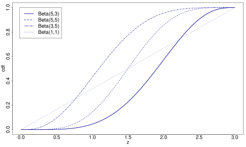
Figure 7: Cumulative Distribution Functions

Finally, we remark that the optimal solution paths are quite nonlinear and they do not have a monotone relationship with underlying parameters in general. For example, we report the optimal delegation and other solutions over the first order stochastic dominant distributions in Table 1. Both sides of the market have the same Beta distribution and we change it according to the first-order stochastic dominance given $A=k=q=1$ and $a=\beta=0.5$. As we can see from Figure 7, the Beta distributions in the table satisfy the first order stochastic dominance relationship: Beta (5,3) first order stochastically dominates Beta (5,5), which first order stochastically dominates Beta (3,5). As the same type distribution on both sides of the market moves to a first-order stochastically dominant distribution, one may expect that $z_{h}$ and $t_{h}$ would increase because there are relatively more high types with a first-order stochastically dominant distribution. However, that’s not the case according to Table 1. The utility indifference conditions, (15) and (16), play the crucial role in determining the upper bound of the reaction interval, but the whole type distributions affect the determination of the upper bound in a non-trivial way through the indifference conditions. Therefore, one cannot say that the planner gives more discretion to receivers as the type distributions on both sides of the market move to first-order stochastically dominant ones.

6 Conclusion

Our studies on optimal delegation provides a noble insight into the principal’s willingness to delegate and the determination of optimal delegation in markets for matching with signaling. We first introduce a new method that shows how to derive an optimal reaction interval for the full implementation of the full implementation of a stronger monotone CSE, the notion of equilibrium adopted from HSS (2023). Choosing an reaction interval is equivalent to choosing the two threshold sender types because we can retrieve the lower and upper bounds of the corresponding interval. Furthermore, the two threshold sender types provide a sharp characterization of a unique stronger monotone CSE.

The relative heterogeneity of receiver types and the productivity of the sender’ signal are crucial in deriving an optimal interval in the presence of the trade-off between matching efficiency and signaling costs. Optimal delegation studied in our paper assumes that there are no transfers between the planner and receivers or between the planner and senders. Optimal delegation can be studied with transfers. One prominent example is delegation with taxation. It would be interesting but perhaps challenging to examine how the presence of taxation alters the planner’s incentives for delegation and her design of optimal delegation.

Appendix

A Proof of Lemma 1

It is clear that if $z_{h}\rightarrow\bar{z},$ $\left\{\hat{\sigma},\hat{\mu},\hat{\tau},\hat{m}\right\}$ converges to the stronger monotone separating equilibrium with the same lower threshold sender type $z_{\ell}$ as the pooling part vanishes. Note that as $z_{h}\rightarrow z_{\ell}$, $\lim_{z_{h}\rightarrow z_{\ell}}t_{h}=t_{\ell}$ and $\lim_{z_{h}\rightarrow z_{\ell}}s_{h}=\tilde{\sigma}(z_{\ell})=s_{\ell}$ because (15) and (16) are satisfied only when $(t_{h},s_{h})=(t_{\ell},\tilde{\sigma}(z_{\ell}))$. Therefore, combining (9) and (10) with (15) and (16) yields that

$$\lim_{z_{h}\rightarrow z_{\ell}}\left[t_{h}-c\left(s_{h},z_{h}\right)\right]=t_{\ell}-c\left(s_{\ell},z_{\ell}\right)=0,$$

$$\lim_{z_{h}\rightarrow z_{\ell}}\left[\mathbb{E}[v(n\left(z_{h}\right),s_{h},z^{\prime})|z^{\prime}\geq z_{h}]-t_{h}\right]=\mathbb{E}[v(n\left(z_{\ell}\right),s_{\ell},z^{\prime})|z^{\prime}\geq z_{\ell}]-t_{\ell}\geq 0,$$

where the inequality holds with equality if $z_{\ell}>\underline{z}.$ The second equality of the first line and the inequality of the second line are a consequence of Theorem 6 in HSS (2023). These imply that $\left\{\hat{\sigma},\hat{\mu},\hat{\tau},\hat{m}\right\}$ converges the stronger monotone pooling equilibrium where $t_{\ell}$ is the single feasible reaction, $z_{\ell}$ is the threshold sender type for market entry and $s_{\ell}$ is the pooled action for senders in the market. Note that when $z_{\ell}=\underline{z},$ we have $s_{\ell}=0$ and $t_{\ell}=0$ in $\left\{\hat{\sigma},\hat{\mu},\hat{\tau},\hat{m}\right\}$ due to Theorem 6 in HSS (2023).

B Proof of Proposition 2

When $z_{\ell}=\underline{z}$, $s_{\ell}=\zeta(\underline{x},\underline{z})=0$ and $t_{\ell}=c\left(\zeta(\underline{x},\underline{z}),\underline{z}\right)=0$. When $t_{\ell}=0,$ $z_{\ell}=\underline{z}$ and $s_{\ell}=\zeta(\underline{x},\underline{z})=0$. Now consider the case with $z_{\ell}\in(\underline{z},\overline{z}).$ First consider case (i) in Assumption 7 in HSS (2023). For any given $z_{\ell}\in(\underline{z},\overline{z}]$, (9) and (10) induce the equation:

$$v\left(n\left(z_{\ell}\right),s,z_{\ell}\right)-c\left(s,z_{\ell}\right)=0.$$ (A1)

If $s=0,$ then the left-hand side of (A1) is positive. As $s\rightarrow\infty,$ the left-hand side approaches $-\infty$ because of Assumption 4 in HSS (2023). Given Assumption 7.(i) in HSS (2023), $v\left(n\left(z_{\ell}\right),s,z_{\ell}\right)$ is positive and it is independent of $s.$ Because $c$ is continuous in $s$ (Assumption 4 in HSS (2023)), it means that there exists a unique $s_{\ell}$ satisfying ((A1). Then, a unique $t_{\ell}$ is determined by either (9) or (10) given $s_{\ell}$ and $z_{\ell}$.

Now consider case (ii) in Assumption 7 in HSS (2023). For any given $z_{\ell}\in(\underline{z},\overline{z})$, the left hand side of (A1) is zero at $s=0.$ However, we cannot have $s_{\ell}=0.$ If $s_{\ell}=0,$ then $t_{\ell}$ must be zero. Then every seller’s utility is zero by entering the market. This implies that every sender will enter the market so $z_{\ell}$ cannot be greater than $\underline{z}$ given our assumption that everyone enters the market if she is indifferent between entering the market and staying out of it.

Because of Assumptions 4 and 5 in HSS (2023), $v-c$ is strictly concave and the left hand side of (A1) approaches $-\infty$ as $s\rightarrow\infty$. Since the left hand side of (A1) is zero at $s=0$, this implies that there exists a unique positive $s_{\ell}$ satisfying (A1). Then, a unique $t_{\ell}$ is determined by either (9) or (10) given $s_{\ell}$ and $z_{\ell}$.

Suppose that the planner chooses $t_{\ell}$, a part of the unique solution $(t_{\ell},s_{\ell})$ that solves (9) and (10) given $z_{\ell}.$ Then, $(z_{\ell},s_{\ell})$ is a unique solution that solves (9) and (10) because of Lemma 7 in HSS (2023).

C Proof of Proposition 3

First consider case (i) in Assumption 7 in HSS (2023). For any given $z_{h}\in\left(z_{\ell},\overline{z}\right)$, (15) and (16) induces the equation:

$$c\left(s,z_{h}\right)-c\left(\tilde{\sigma}\left(z_{h}\right),z_{h}\right)=\mathbb{E}[v(n\left(z_{h}\right),s,z^{\prime})|z^{\prime}\geq z_{h}]-v\left(n\left(z_{h}\right),\tilde{\sigma}\left(z_{h}\right),z_{h}\right).$$ (A2)

The right hand side of (A2) is positive because it is independent of $s$ and $\tilde{\sigma}\left(z_{h}\right)$ and $z^{\prime}\geq z_{h}$ for $z_{h}<\overline{z}.$ The left-hand side is continuous and increasing in $s$. Because of Assumptions 1.(i) and 4, the left hand side is increasing in $s$ with $\lim_{s\searrow 0}\left[c\left(s,z_{h}\right)-c\left(\tilde{\sigma}\left(z_{h}\right),z_{h}\right)\right]<0$ and $\lim_{s\nearrow\infty}\left[c\left(s,z_{h}\right)-c\left(\tilde{\sigma}\left(z_{h}\right),z_{h}\right)\right]=\infty.$ Therefore, we have a unique solution for $s_{h}$ that solves (A2). Then, $t_{h}$ can be uniquely derived from either (15) and (16). Therefore, for any given $z_{h}\in\left(z_{\ell},\overline{z}\right),$ there exists a unique $(t_{h},s_{h})$ that satisfies (15) and (16).

Now consider case (ii) in Assumption 7 in HSS (2023). For any given $z_{h}\in\left(z_{\ell},\overline{z}\right),$ (15) and (16) induce the equation:

$$\mathbb{E}[v(n\left(z_{h}\right),s,z^{\prime})|z^{\prime}\geq z_{h}]-c\left(s,z_{h}\right)=v\left(n\left(z_{h}\right),\tilde{\sigma}\left(z_{h}\right),z_{h}\right)-c\left(\tilde{\sigma}\left(z_{h}\right),z_{h}\right).$$ (A3)

The right hand side of (A3) is positive because it is the sum of the equilibrium utilities for the sender type $z_{h}$ and the receiver type $n\left(z_{h}\right)$ for $z_{h}\in\left(z_{\ell},\overline{z}\right)$ in the stronger monotone separating equilibrium and both equilibrium utilities for senders and receivers are increasing in types in the separating equilibrium. Because of Assumption 4 ($c\left(0,z\right)=0$ for all $z$) and case (ii) in Assumption 7 ($v(x,0,z)=0$ for all $x$ and $z$) in HSS (2023), we have that

$$0=\mathbb{E}[v(n\left(z_{h}\right),0,z^{\prime})|z^{\prime}\geq z_{h}]-c\left(0,z_{h}\right)<v\left(n\left(z_{h}\right),\tilde{\sigma}\left(z_{h}\right),z_{h}\right)-c\left(\tilde{\sigma}\left(z_{h}\right),z_{h}\right)$$ (A4)

Because of Assumption 5 ($\lim_{s\rightarrow\infty}v_{s}(x,s,z)=0$ given any $x$ and $z$ and $\lim_{s\rightarrow\infty}$ $c_{s}(s,z)=\infty$ given any $z$) in HSS (2023), we have that

$$-\infty=\lim_{s\rightarrow\infty}\left[\mathbb{E}[v(n\left(z_{h}\right),s,z^{\prime})|z^{\prime}\geq z_{h}]-c\left(s,z_{h}\right)\right]<v\left(n\left(z_{h}\right),\tilde{\sigma}\left(z_{h}\right),z_{h}\right)-c\left(\tilde{\sigma}\left(z_{h}\right),z_{h}\right)$$ (A5)

When $s=\tilde{\sigma}\left(z_{h}\right)$, we have that

$$\mathbb{E}[v(n\left(z_{h}\right),\tilde{\sigma}\left(z_{h}\right),z^{\prime})|z^{\prime}\geq z_{h}]-c\left(\tilde{\sigma}\left(z_{h}\right),z_{h}\right)>v\left(n\left(z_{h}\right),\tilde{\sigma}\left(z_{h}\right),z_{h}\right)-c\left(\tilde{\sigma}\left(z_{h}\right),z_{h}\right).$$ (A6)

because $\mathbb{E}[v(n\left(z_{h}\right),\tilde{\sigma}\left(z_{h}\right),z^{\prime})|z^{\prime}\geq z_{h}]>v\left(n\left(z_{h}\right),\tilde{\sigma}\left(z_{h}\right),z_{h}\right).$

Because $\mathbb{E}[v(n\left(z_{h}\right),s,z^{\prime})|z^{\prime}\geq z_{h}]-c\left(s,z_{h}\right)$ is strictly concave in $s$ due to Assumption 5 in HSS (2023), (A4), (A5), and (A6) imply that there are two values, $s^{0}$ and $s^{1}$ that satisfy (A3) with $s^{0}<\tilde{\sigma}\left(z_{h}\right)<s^{1}$. Because $\tilde{\sigma}\left(z_{h}\right)<s_{h}$ from Lemma 13 in HSS (2023), $s_{h}$ is equal to $s^{1}$. Because $t_{h}$ can be uniquely derived from either (15) and (16), there exists a unique $(t_{h},s_{h})$ that satisfies (15) and (16) for any given $z_{h}\in\left(z_{\ell},\overline{z}\right).$ Therefore, in both cases in Assumption 7 in HSS (2023), there exists a unique $t_{h}$ and a unique $s_{h}$ that satisfies (15) and (16) for any given $z_{h}\in\left(z_{\ell},\overline{z}\right)$. Suppose that the planner chooses $t_{h}$, a part of the unique solution $(t_{h},s_{h})$ that solves (15) and (16) given $z_{h}\in\left(z_{\ell},\overline{z}\right)$. Then, $(z_{h},s_{h})$ is a unique solution that solves (15) and (16) because of Lemma 12.

Because all functions in (15) and (16) are continuous (Assumptions 3.(ii), 4.(i), 6.(ii) and Theorem 4 in HSS (2023)), it is clear the solution $(t_{h},s_{h})$ is continuous in $z_{h}$ and that $z_{h}$, the part of the solution ($z_{h},s_{h})$ is also continuous in $t_{h}.$ Finally, $\lim_{z_{h}\rightarrow z_{\ell}}t_{h}=t_{\ell}$ and $\lim_{z_{h}\rightarrow z_{\ell}}s_{h}=\tilde{\sigma}\left(z_{\ell}\right)$ because (15) and (16) are satisfied only when $(t_{h},s)=(t_{\ell},\tilde{\sigma}\left(z_{\ell}\right))$ as $z_{h}\rightarrow\underline{z}$.

D Proof of Proposition 4

Consider the initial value problem:

$$\left\{\begin{array}[]{cc}v_{s}(n(\mu(s)),s,\mu(s))+v_{z}(n(\mu(s)),s,\mu(s))\mu^{\prime}(s)-c_{s}(s,\mu(s))=0&\\ \mu(s_{\ell})=z_{\ell}&\end{array}\right.\text{ }.$$

Given $v(x,s,z)=As^{a}xz$,  $c(s,z)=\beta\dfrac{s^{2}}{z}$,  and $n(z)=kz^{q}$, we have that $v_{z}(x,s,z)=As^{a}x$,  $v_{s}(x,s,z)=aAs^{a-1}xz$, and $c_{s}(s,z)=2\beta\dfrac{s}{z}$. Therefore, the above IVP becomes

$$aAs^{a-1}k\mu(s)^{q}\mu(s)+As^{a}k\mu(s)^{q}\mu^{\prime}(s)-\dfrac{2\beta s}{\mu(s)}=0.$$ (A7)

Rewriting (A7) gives

$$\dfrac{Ak}{2\beta}\mu(s)^{1+q}\mu^{\prime}(s)+\dfrac{aAk}{2\beta s}\mu(s)^{2+q}=s^{1-a}.$$ (A8)

Let $D=:\dfrac{Ak}{2\beta}$. Thus, (A8) becomes

$$D\mu^{1+q}\mu^{\prime}+\dfrac{aD}{s}\mu^{2+q}=s^{1-a}$$ (A9)

where we denote $\mu=:\mu(s)$ for simplicity. Let $v=\mu^{2+q}$. Then $v^{\prime}=(2+q)\mu^{1+q}\mu^{\prime}$ and (A9) becomes

$$v^{\prime}+\dfrac{a(2+q)}{s}v=\left(\dfrac{2+q}{D}\right)s^{1-a}$$ (A10)

which is a first order linear differential equation with integrating factor $\mathcal{I}(s)=s^{a(2+q)}$. Therefore, (A10) is equivalent to $\frac{d}{ds}\left\{vs^{a(2+q)}\right\}=\left(\dfrac{2+q}{D}\right)s^{1+a+aq},$ which implies

$$vs^{a(2+q)}=\left(\dfrac{2+q}{D}\right)\int s^{1+a+aq}ds+\kappa,$$ (A11)

where $\kappa$ is some integration constant. Equation (A11) implies

$$\mu(s)^{2+q}=\left(\dfrac{2+q}{D}\right)\left(\dfrac{s^{2-a}}{2+a+aq}\right)+\dfrac{\kappa}{s^{a(2+q)}}.$$ (A12)

given that $v=\mu^{2+q}$. By using the initial condition $\mu(s_{\ell})=z_{\ell}$, we compute $\kappa$ as follows:

$$z_{\ell}^{2+q}=\left(\dfrac{2+q}{D}\right)\left(\dfrac{s_{\ell}^{2-a}}{2+a+aq}\right)+\dfrac{\kappa}{s_{\ell}^{a(2+q)}}$$ (A13)

which gives

$$\kappa=\dfrac{s_{\ell}^{a(2+q)}\left[D(2+a+aq)z_{\ell}^{2+q}-(2+q)s_{\ell}^{(2-a)}\right]}{D(2+a+aq)}.$$ (A14)

Plugging (A14) into (A12) gives

$$\tilde{\mu}(s)=\left[\left(\dfrac{2\beta(2+q)}{Ak}\right)\dfrac{s^{2-a}}{2+a+aq}+\left(\dfrac{s_{\ell}}{s}\right)^{a(2+q)}\dfrac{\left[Ak(2+a+aq)z_{\ell}^{2+q}-2\beta(2+q)s_{\ell}^{(2-a)}\right]}{Ak(2+a+aq)}\right]^{\dfrac{1}{2+q}},$$ (A15)

where $s_{\ell}$ is determined by (17) and it is $s_{\ell}(z_{\ell})=\left(\frac{Ak}{\beta}z_{\ell}^{q+2}\right)^{\frac{1}{2-a}}.$

E Proof of Proposition 3

First, we construct a (unique) stronger monotone pooling equilibrium with a positive single feasible reaction $t^{\ast}>0$. Because (13) and (14) must hold with equality by Theorem 6 in HSS (2023) with $z^{\ast}>\underline{z}$, the pooled action $s^{\ast}(z^{\ast},q,a)$ solves $As^{\ast}{}^{a}kz^{\ast}{}^{q}\mathbb{E}\left[z|z\geq z^{\ast}\right]-\beta\frac{s^{\ast}{}^{2}}{z^{\ast}}=0$ and hence we have that $s^{\ast}(z^{\ast},q,a)=\left(\frac{z^{\ast q+1}Ak\mathbb{E}\left[z|z\geq z^{\ast}\right]}{\beta}\right)^{\frac{1}{2-a}}$. Therefore, we have that $\lim_{q,a\rightarrow 0}s^{\ast}(t,q,a)=\sqrt{z^{\ast}Ak\mathbb{E}\left[z|z\geq z^{\ast}\right]/\beta}.$

The aggregate net surplus in the stronger monotone pooling equilibrium is

$$\Pi_{p}(z^{\ast},q,a,G):=\int_{z^{\ast}}^{\bar{z}}As^{\ast}(z^{\ast},q,a)^{a}kz^{\ast q}\mathbb{E}\left[z|z\geq z^{\ast}\right]dG(z)-\beta s^{\ast}(z^{\ast},q,a)^{2}\int_{z^{\ast}}^{\bar{z}}\frac{1}{z}dG(z).$$

This implies that

$$\lim_{q,a\rightarrow 0}\Pi_{p}(z^{\ast},q,a,G)=\int_{z^{\ast}}^{\bar{z}}Ak\mathbb{E}\left[z|z\geq z^{\ast}\right]dG(z)-z^{\ast}Ak\mathbb{E}\left[z|z\geq z^{\ast}\right]\int_{z^{\ast}}^{\bar{z}}\frac{1}{z}dG(z),$$

$$\lim_{z^{\ast}\rightarrow 0}\left[\lim_{q,a\rightarrow 0}\Pi_{p}(z^{\ast},q,a,G)\right]=\int_{0}^{\bar{z}}Ak\mu_{z}dG(z)=Ak\mu_{z}$$

where $\mu_{z}$ is the unconditional mean of the sender type $z.$ Because $\lim_{q,a\rightarrow 0}\Pi^{\ast}(q,a,G)=\frac{Ak\mu_{z}}{2}$, we have that

$$\lim_{z^{\ast}\rightarrow 0}\left[\lim_{q,a\rightarrow 0}\Pi_{p}(z^{\ast},q,a,G)\right]-\lim_{q,a\rightarrow 0}\Pi_{\ast}(q,a,G)=\frac{Ak\mu_{z}}{2}>0.$$ (A16)

Because $\Pi_{p}(z^{\ast},q,a,G)$ and $\Pi_{\ast}(q,a,G)$ are continuous, there exists $\tilde{q}>0$, and $\tilde{a}>0$ and $z^{\ast}(\tilde{q},\tilde{a})\in$ Int $Z$ such that for every $(q,a)\in[0,\tilde{q}]\times[0,\tilde{a}]$ and every $z^{\ast}\in(0,z^{\ast}(\tilde{q},\tilde{a})]$, $\Pi_{p}(z^{\ast},q,a,G)>\Pi_{s}(q,a,G)$. We can retrieve $t^{\ast}>0$ given $z^{\ast}\in(0,z^{\ast}(\tilde{q},\tilde{a})]$.

F Additional Figures and Tables

F.1 Figures

Figure 8: Design 4. Change of Signal Contribution ($a$) and Receiver Type ($k$)

Beta(1,1)
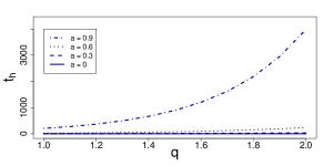
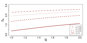
Beta(3,5)
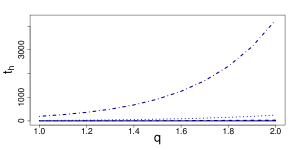
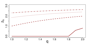
Beta(5,5)
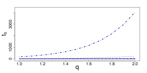
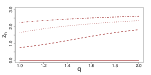
Beta(5,3)

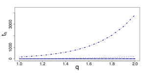
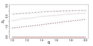
• Notes. This design varies both the signal contribution parameter $a$ and the distribution of the receiver type by $q$. Recall the matching function $x=kz^{q}$ and the match surplus function $v(x,s,z)=As^{a}xz$. We keep the same distribution on senders’ type. The lower bound of an interval delegation is always zero ($t_{l}=0$). The lower bound of a well-behaved equilibrium is also zero ($z_{l}=0$).

F.2 Tables

Table 2: Design 1 with Beta(1,1)

$q$	$k$	$\bar{z}$	$\bar{x}$	$t_{h}$	$z_{h}$	$x_{h}$	$s_{h}$
1.00	1.00	1.00	1.00	0.41	0.58	0.58	0.53
1.00	1.00	1.20	1.20	0.74	0.70	0.70	0.76
1.00	1.00	1.40	1.40	1.22	0.82	0.82	1.03
1.00	1.00	1.60	1.60	1.89	0.94	0.94	1.34
1.00	1.00	1.80	1.80	2.78	1.05	1.05	1.70
1.00	1.00	2.00	2.00	3.94	1.17	1.17	2.10
1.00	1.00	2.20	2.20	5.41	1.29	1.29	2.54
1.00	1.00	2.40	2.40	7.24	1.40	1.40	3.03
1.00	1.00	2.60	2.60	9.47	1.52	1.52	3.55
1.00	1.00	2.80	2.80	12.18	1.64	1.64	4.12
1.00	1.00	3.00	3.00	15.40	1.75	1.75	4.73

Table 3: Design 1 with Beta(5,5)

$q$	$k$	$\bar{z}$	$\bar{x}$	$t_{h}$	$z_{h}$	$x_{h}$	$s_{h}$
1.00	1.00	1.00	1.00	0.17	0.45	0.45	0.30
1.00	1.00	1.20	1.20	0.30	0.54	0.54	0.43
1.00	1.00	1.40	1.40	0.50	0.62	0.62	0.58
1.00	1.00	1.60	1.60	0.76	0.71	0.71	0.76
1.00	1.00	1.80	1.80	1.12	0.80	0.80	0.97
1.00	1.00	2.00	2.00	1.58	0.89	0.89	1.19
1.00	1.00	2.20	2.20	2.15	0.98	0.98	1.45
1.00	1.00	2.40	2.40	2.87	1.07	1.07	1.72
1.00	1.00	2.60	2.60	3.74	1.16	1.16	2.02
1.00	1.00	2.80	2.80	4.79	1.25	1.25	2.34
1.00	1.00	3.00	3.00	6.03	1.34	1.34	2.69

Table 4: Design 1 with Beta(3,5)

$q$	$k$	$\bar{z}$	$\bar{x}$	$t_{h}$	$z_{h}$	$x_{h}$	$s_{h}$
1.00	1.00	1.00	1.00	0.27	0.54	0.54	0.37
1.00	1.00	1.20	1.20	0.48	0.65	0.65	0.54
1.00	1.00	1.40	1.40	0.79	0.76	0.76	0.73
1.00	1.00	1.60	1.60	1.22	0.86	0.86	0.96
1.00	1.00	1.80	1.80	1.81	0.97	0.97	1.21
1.00	1.00	2.00	2.00	2.57	1.08	1.08	1.50
1.00	1.00	2.20	2.20	3.54	1.19	1.19	1.81
1.00	1.00	2.40	2.40	4.76	1.30	1.30	2.15
1.00	1.00	2.60	2.60	6.25	1.40	1.40	2.53
1.00	1.00	2.80	2.80	8.05	1.51	1.51	2.93
1.00	1.00	3.00	3.00	10.21	1.62	1.62	3.37

Table 5: Design 1 with Beta(5,3)

$q$	$k$	$\bar{z}$	$\bar{x}$	$t_{h}$	$z_{h}$	$x_{h}$	$s_{h}$
1.00	1.00	1.00	1.00	0.20	0.45	0.45	0.34
1.00	1.00	1.20	1.20	0.36	0.54	0.54	0.49
1.00	1.00	1.40	1.40	0.59	0.63	0.63	0.67
1.00	1.00	1.60	1.60	0.90	0.72	0.72	0.88
1.00	1.00	1.80	1.80	1.31	0.81	0.81	1.11
1.00	1.00	2.00	2.00	1.84	0.90	0.90	1.37
1.00	1.00	2.20	2.20	2.51	0.99	0.99	1.66
1.00	1.00	2.40	2.40	3.33	1.08	1.08	1.98
1.00	1.00	2.60	2.60	4.33	1.17	1.17	2.32
1.00	1.00	2.80	2.80	5.53	1.25	1.25	2.69
1.00	1.00	3.00	3.00	6.94	1.34	1.34	3.09

Table 6: Design 2 with Beta(1,1)

$q$	$k$	$\bar{z}$	$\bar{x}$	$t_{h}$	$z_{h}$	$x_{h}$	$s_{h}$
1.00	1.00	3.00	3.00	15.40	1.75	1.75	4.73
1.00	1.20	3.00	3.60	20.68	1.75	2.11	5.34
1.00	1.40	3.00	4.20	26.61	1.75	2.46	5.92
1.00	1.60	3.00	4.80	33.17	1.75	2.81	6.47
1.00	1.80	3.00	5.40	40.36	1.75	3.16	7.00
1.00	2.00	3.00	6.00	48.16	1.75	3.51	7.51
1.00	2.20	3.00	6.60	56.57	1.75	3.86	8.00
1.00	2.40	3.00	7.20	65.58	1.75	4.21	8.48
1.00	2.60	3.00	7.80	75.19	1.75	4.56	8.94
1.00	2.80	3.00	8.40	85.39	1.75	4.91	9.39
1.00	3.00	3.00	9.00	96.18	1.75	5.26	9.84

Table 7: Design 2 with Beta(5,5)

$q$	$k$	$\bar{z}$	$\bar{x}$	$t_{h}$	$z_{h}$	$x_{h}$	$s_{h}$
1.00	1.00	3.00	3.00	6.03	1.34	1.34	2.69
1.00	1.20	3.00	3.60	8.04	1.34	1.61	3.03
1.00	1.40	3.00	4.20	10.29	1.34	1.87	3.36
1.00	1.60	3.00	4.80	12.76	1.34	2.14	3.67
1.00	1.80	3.00	5.40	15.45	1.34	2.41	3.98
1.00	2.00	3.00	6.00	18.36	1.34	2.68	4.26
1.00	2.20	3.00	6.60	21.48	1.34	2.94	4.54
1.00	2.40	3.00	7.20	24.82	1.34	3.21	4.82
1.00	2.60	3.00	7.80	28.36	1.34	3.48	5.08
1.00	2.80	3.00	8.40	32.12	1.34	3.75	5.34
1.00	3.00	3.00	9.00	36.08	1.34	4.01	5.59

Table 8: Design 2 with Beta(3,5)

$q$	$k$	$\bar{z}$	$\bar{x}$	$t_{h}$	$z_{h}$	$x_{h}$	$s_{h}$
1.00	1.00	3.00	3.00	10.21	1.62	1.62	3.37
1.00	1.20	3.00	3.60	13.78	1.62	1.94	3.80
1.00	1.40	3.00	4.20	17.80	1.62	2.27	4.21
1.00	1.60	3.00	4.80	22.27	1.62	2.59	4.61
1.00	1.80	3.00	5.40	27.18	1.62	2.92	4.98
1.00	2.00	3.00	6.00	32.52	1.62	3.24	5.34
1.00	2.20	3.00	6.60	38.29	1.62	3.56	5.70
1.00	2.40	3.00	7.20	44.49	1.62	3.89	6.04
1.00	2.60	3.00	7.80	51.12	1.62	4.21	6.37
1.00	2.80	3.00	8.40	58.16	1.62	4.54	6.69
1.00	3.00	3.00	9.00	65.62	1.62	4.86	7.00

Table 9: Design 2 with Beta(5,3)

$q$	$k$	$\bar{z}$	$\bar{x}$	$t_{h}$	$z_{h}$	$x_{h}$	$s_{h}$
1.00	1.00	3.00	3.00	6.94	1.34	1.34	3.09
1.00	1.20	3.00	3.60	9.21	1.34	1.61	3.49
1.00	1.40	3.00	4.20	11.73	1.34	1.88	3.87
1.00	1.60	3.00	4.80	14.49	1.34	2.15	4.22
1.00	1.80	3.00	5.40	17.48	1.34	2.42	4.57
1.00	2.00	3.00	6.00	20.71	1.34	2.69	4.90
1.00	2.20	3.00	6.60	24.17	1.34	2.96	5.22
1.00	2.40	3.00	7.20	27.85	1.34	3.23	5.54
1.00	2.60	3.00	7.80	31.75	1.34	3.50	5.84
1.00	2.80	3.00	8.40	35.87	1.34	3.76	6.14
1.00	3.00	3.00	9.00	40.21	1.34	4.03	6.42

Table 10: Design 3 with Beta(1,1)

$q$	$k$	$\bar{z}$	$\bar{x}$	$t_{h}$	$z_{h}$	$x_{h}$	$s_{h}$
1.00	1.00	3.00	3.00	15.40	1.75	1.75	4.73
1.10	1.00	3.00	3.35	18.85	1.83	1.94	5.16
1.20	1.00	3.00	3.74	23.09	1.89	2.15	5.62
1.30	1.00	3.00	4.17	28.30	1.95	2.38	6.12
1.40	1.00	3.00	4.66	34.72	2.00	2.65	6.65
1.50	1.00	3.00	5.20	42.63	2.05	2.94	7.21
1.60	1.00	3.00	5.80	52.37	2.10	3.28	7.82
1.70	1.00	3.00	6.47	64.39	2.14	3.65	8.47
1.80	1.00	3.00	7.22	79.22	2.18	4.08	9.17
1.90	1.00	3.00	8.06	97.56	2.22	4.55	9.92
2.00	1.00	3.00	9.00	120.23	2.25	5.08	10.72

Table 11: Design 3 with Beta(5,5)

$q$	$k$	$\bar{z}$	$\bar{x}$	$t_{h}$	$z_{h}$	$x_{h}$	$s_{h}$
1.00	1.00	3.00	3.00	6.03	1.34	1.34	2.69
1.10	1.00	3.00	3.35	8.48	1.48	1.54	3.15
1.20	1.00	3.00	3.74	11.80	1.61	1.77	3.65
1.30	1.00	3.00	4.17	16.16	1.72	2.03	4.18
1.40	1.00	3.00	4.66	21.74	1.82	2.32	4.75
1.50	1.00	3.00	5.20	28.83	1.91	2.64	5.34
1.60	1.00	3.00	5.80	37.78	1.99	3.00	5.96
1.70	1.00	3.00	6.47	49.06	2.05	3.40	6.62
1.80	1.00	3.00	7.22	63.23	2.11	3.85	7.32
1.90	1.00	3.00	8.06	81.00	2.17	4.34	8.06
2.00	1.00	3.00	9.00	103.29	2.21	4.90	8.85

Table 12: Design 3 with Beta(3,5)

$q$	$k$	$\bar{z}$	$\bar{x}$	$t_{h}$	$z_{h}$	$x_{h}$	$s_{h}$
1.00	1.00	3.00	3.00	10.21	1.62	1.62	3.37
1.10	1.00	3.00	3.35	13.53	1.73	1.82	3.83
1.20	1.00	3.00	3.74	17.70	1.82	2.05	4.31
1.30	1.00	3.00	4.17	22.91	1.90	2.31	4.81
1.40	1.00	3.00	4.66	29.41	1.98	2.59	5.35
1.50	1.00	3.00	5.20	37.53	2.04	2.91	5.91
1.60	1.00	3.00	5.80	47.66	2.10	3.27	6.51
1.70	1.00	3.00	6.47	60.27	2.15	3.67	7.15
1.80	1.00	3.00	7.22	75.99	2.20	4.12	7.83
1.90	1.00	3.00	8.06	95.57	2.24	4.63	8.56
2.00	1.00	3.00	9.00	119.98	2.28	5.20	9.33

Table 13: Design 3 with Beta(5,3)

$q$	$k$	$\bar{z}$	$\bar{x}$	$t_{h}$	$z_{h}$	$x_{h}$	$s_{h}$
1.00	1.00	3.00	3.00	6.94	1.34	1.34	3.09
1.10	1.00	3.00	3.35	8.89	1.45	1.51	3.46
1.20	1.00	3.00	3.74	11.54	1.55	1.70	3.89
1.30	1.00	3.00	4.17	15.08	1.66	1.93	4.37
1.40	1.00	3.00	4.66	19.72	1.75	2.19	4.89
1.50	1.00	3.00	5.20	25.74	1.83	2.48	5.45
1.60	1.00	3.00	5.80	33.48	1.91	2.82	6.05
1.70	1.00	3.00	6.47	43.33	1.98	3.20	6.70
1.80	1.00	3.00	7.22	55.84	2.04	3.62	7.39
1.90	1.00	3.00	8.06	71.66	2.10	4.10	8.13
2.00	1.00	3.00	9.00	91.60	2.15	4.64	8.93

Table 14: Design 4 with Beta(1,1)

$q$	$k$	$a$	$\bar{z}$	$\bar{x}$	$t_{h}$	$z_{h}$	$x_{h}$	$s_{h}$
1.00	1.00	0.00	3.00	3.00	0.57	0.38	0.38	0.65
1.10	1.00	0.00	3.00	3.35	0.66	0.47	0.44	0.77
1.20	1.00	0.00	3.00	3.74	0.77	0.56	0.50	0.89
1.30	1.00	0.00	3.00	4.17	0.89	0.65	0.57	1.01
1.40	1.00	0.00	3.00	4.66	1.02	0.73	0.64	1.13
1.50	1.00	0.00	3.00	5.20	1.18	0.81	0.73	1.25
1.60	1.00	0.00	3.00	5.80	1.36	0.89	0.82	1.38
1.70	1.00	0.00	3.00	6.47	1.58	0.96	0.93	1.51
1.80	1.00	0.00	3.00	7.22	1.83	1.02	1.04	1.64
1.90	1.00	0.00	3.00	8.06	2.12	1.09	1.18	1.78
2.00	1.00	0.00	3.00	9.00	2.46	1.15	1.32	1.92
1.00	1.00	0.30	3.00	3.00	5.90	1.36	1.36	2.77
1.10	1.00	0.30	3.00	3.35	7.04	1.44	1.50	3.01
1.20	1.00	0.30	3.00	3.74	8.41	1.52	1.65	3.28
1.30	1.00	0.30	3.00	4.17	10.05	1.59	1.83	3.55
1.40	1.00	0.30	3.00	4.66	12.01	1.66	2.03	3.85
1.50	1.00	0.30	3.00	5.20	14.36	1.72	2.26	4.15
1.60	1.00	0.30	3.00	5.80	17.18	1.78	2.51	4.48
1.70	1.00	0.30	3.00	6.47	20.56	1.83	2.80	4.82
1.80	1.00	0.30	3.00	7.22	24.62	1.88	3.13	5.19
1.90	1.00	0.30	3.00	8.06	29.48	1.93	3.49	5.58
2.00	1.00	0.30	3.00	9.00	35.33	1.97	3.90	5.99
1.00	1.00	0.60	3.00	3.00	26.02	1.92	1.92	6.19
1.10	1.00	0.60	3.00	3.35	32.37	1.98	2.12	6.77
1.20	1.00	0.60	3.00	3.74	40.31	2.04	2.35	7.40
1.30	1.00	0.60	3.00	4.17	50.24	2.09	2.61	8.08
1.40	1.00	0.60	3.00	4.66	62.68	2.14	2.90	8.81
1.50	1.00	0.60	3.00	5.20	78.26	2.18	3.23	9.60
1.60	1.00	0.60	3.00	5.80	97.80	2.22	3.59	10.45
1.70	1.00	0.60	3.00	6.47	122.34	2.26	4.01	11.37
1.80	1.00	0.60	3.00	7.22	153.17	2.30	4.47	12.36
1.90	1.00	0.60	3.00	8.06	191.95	2.33	4.99	13.44
2.00	1.00	0.60	3.00	9.00	240.76	2.36	5.57	14.59
1.00	1.00	0.90	3.00	3.00	206.64	2.29	2.29	15.92
1.10	1.00	0.90	3.00	3.35	276.32	2.34	2.54	17.74
1.20	1.00	0.90	3.00	3.74	369.97	2.38	2.82	19.73
1.30	1.00	0.90	3.00	4.17	495.99	2.41	3.14	21.94
1.40	1.00	0.90	3.00	4.66	665.73	2.45	3.50	24.38
1.50	1.00	0.90	3.00	5.20	894.60	2.48	3.89	27.07
1.60	1.00	0.90	3.00	5.80	1203.39	2.50	4.34	30.05
1.70	1.00	0.90	3.00	6.47	1620.49	2.53	4.84	33.34
1.80	1.00	0.90	3.00	7.22	2184.06	2.55	5.40	36.97
1.90	1.00	0.90	3.00	8.06	2946.38	2.57	6.03	40.99
2.00	1.00	0.90	3.00	9.00	3977.63	2.59	6.73	45.44

Table 15: Design 4 with Beta(5,5)

$q$	$k$	$a$	$\bar{z}$	$\bar{x}$	$t_{h}$	$z_{h}$	$x_{h}$	$s_{h}$
1.00	1.00	0.00	3.00	3.00	0.00	0.00	0.00	0.00
1.10	1.00	0.00	3.00	3.35	0.00	0.00	0.00	0.00
1.20	1.00	0.00	3.00	3.74	0.00	0.00	0.00	0.00
1.30	1.00	0.00	3.00	4.17	0.00	0.00	0.00	0.00
1.40	1.00	0.00	3.00	4.66	0.00	0.00	0.00	0.00
1.50	1.00	0.00	3.00	5.20	0.00	0.00	0.00	0.00
1.60	1.00	0.00	3.00	5.80	0.00	0.00	0.00	0.00
1.70	1.00	0.00	3.00	6.47	0.00	0.00	0.00	0.00
1.80	1.00	0.00	3.00	7.22	0.00	0.00	0.00	0.00
1.90	1.00	0.00	3.00	8.06	0.00	0.00	0.00	0.00
2.00	1.00	0.00	3.00	9.00	0.00	0.00	0.00	0.00
1.00	1.00	0.30	3.00	3.00	1.51	0.76	0.76	1.21
1.10	1.00	0.30	3.00	3.35	1.79	0.84	0.83	1.34
1.20	1.00	0.30	3.00	3.74	2.20	0.94	0.93	1.50
1.30	1.00	0.30	3.00	4.17	2.85	1.05	1.07	1.71
1.40	1.00	0.30	3.00	4.66	3.82	1.17	1.25	1.98
1.50	1.00	0.30	3.00	5.20	5.25	1.30	1.48	2.29
1.60	1.00	0.30	3.00	5.80	7.24	1.42	1.76	2.65
1.70	1.00	0.30	3.00	6.47	9.87	1.54	2.08	3.03
1.80	1.00	0.30	3.00	7.22	13.24	1.64	2.44	3.43
1.90	1.00	0.30	3.00	8.06	17.48	1.73	2.84	3.86
2.00	1.00	0.30	3.00	9.00	22.74	1.81	3.29	4.30
1.00	1.00	0.60	3.00	3.00	13.56	1.64	1.64	4.06
1.10	1.00	0.60	3.00	3.35	18.87	1.76	1.87	4.69
1.20	1.00	0.60	3.00	3.74	25.78	1.87	2.12	5.36
1.30	1.00	0.60	3.00	4.17	34.68	1.96	2.39	6.06
1.40	1.00	0.60	3.00	4.66	46.10	2.03	2.70	6.80
1.50	1.00	0.60	3.00	5.20	60.70	2.10	3.05	7.60
1.60	1.00	0.60	3.00	5.80	79.34	2.16	3.43	8.44
1.70	1.00	0.60	3.00	6.47	103.09	2.22	3.87	9.34
1.80	1.00	0.60	3.00	7.22	133.36	2.26	4.35	10.31
1.90	1.00	0.60	3.00	8.06	171.88	2.31	4.89	11.35
2.00	1.00	0.60	3.00	9.00	220.90	2.34	5.50	12.46
1.00	1.00	0.90	3.00	3.00	169.09	2.24	2.24	12.95
1.10	1.00	0.90	3.00	3.35	235.88	2.30	2.50	14.70
1.20	1.00	0.90	3.00	3.74	327.14	2.35	2.79	16.62
1.30	1.00	0.90	3.00	4.17	451.61	2.40	3.11	18.73
1.40	1.00	0.90	3.00	4.66	621.34	2.44	3.48	21.06
1.50	1.00	0.90	3.00	5.20	852.53	2.47	3.89	23.62
1.60	1.00	0.90	3.00	5.80	1167.55	2.50	4.34	26.45
1.70	1.00	0.90	3.00	6.47	1596.11	2.53	4.86	29.57
1.80	1.00	0.90	3.00	7.22	2179.49	2.56	5.43	33.02
1.90	1.00	0.90	3.00	8.06	2972.88	2.58	6.07	36.83
2.00	1.00	0.90	3.00	9.00	4052.01	2.61	6.79	41.04

Table 16: Design 4 with Beta(3,5)

$q$	$k$	$a$	$\bar{z}$	$\bar{x}$	$t_{h}$	$z_{h}$	$x_{h}$	$s_{h}$
1.00	1.00	0.00	3.00	3.00	0.00	0.00	0.00	0.00
1.10	1.00	0.00	3.00	3.35	0.00	0.00	0.00	0.00
1.20	1.00	0.00	3.00	3.74	0.00	0.00	0.00	0.00
1.30	1.00	0.00	3.00	4.17	0.00	0.00	0.00	0.00
1.40	1.00	0.00	3.00	4.66	0.00	0.00	0.00	0.00
1.50	1.00	0.00	3.00	5.20	0.00	0.00	0.00	0.00
1.60	1.00	0.00	3.00	5.80	0.00	0.00	0.00	0.00
1.70	1.00	0.00	3.00	6.47	0.00	0.00	0.00	0.00
1.80	1.00	0.00	3.00	7.22	0.00	0.00	0.00	0.00
1.90	1.00	0.00	3.00	8.06	0.33	0.59	0.36	0.58
2.00	1.00	0.00	3.00	9.00	0.63	0.80	0.64	0.87
1.00	1.00	0.30	3.00	3.00	2.37	1.01	1.01	1.49
1.10	1.00	0.30	3.00	3.35	3.29	1.16	1.17	1.77
1.20	1.00	0.30	3.00	3.74	4.50	1.29	1.36	2.06
1.30	1.00	0.30	3.00	4.17	6.03	1.42	1.57	2.37
1.40	1.00	0.30	3.00	4.66	7.93	1.52	1.80	2.70
1.50	1.00	0.30	3.00	5.20	10.27	1.62	2.07	3.03
1.60	1.00	0.30	3.00	5.80	13.15	1.71	2.36	3.37
1.70	1.00	0.30	3.00	6.47	16.65	1.79	2.68	3.73
1.80	1.00	0.30	3.00	7.22	20.92	1.86	3.04	4.11
1.90	1.00	0.30	3.00	8.06	26.12	1.92	3.45	4.50
2.00	1.00	0.30	3.00	9.00	32.45	1.98	3.90	4.92
1.00	1.00	0.60	3.00	3.00	19.65	1.84	1.84	4.73
1.10	1.00	0.60	3.00	3.35	25.90	1.93	2.06	5.33
1.20	1.00	0.60	3.00	3.74	33.83	2.00	2.30	5.96
1.30	1.00	0.60	3.00	4.17	43.89	2.07	2.58	6.63
1.40	1.00	0.60	3.00	4.66	56.64	2.13	2.89	7.36
1.50	1.00	0.60	3.00	5.20	72.78	2.19	3.23	8.13
1.60	1.00	0.60	3.00	5.80	93.22	2.24	3.62	8.95
1.70	1.00	0.60	3.00	6.47	119.11	2.28	4.06	9.84
1.80	1.00	0.60	3.00	7.22	151.89	2.32	4.54	10.80
1.90	1.00	0.60	3.00	8.06	193.38	2.36	5.09	11.83
2.00	1.00	0.60	3.00	9.00	245.96	2.39	5.70	12.93
1.00	1.00	0.90	3.00	3.00	193.76	2.30	2.30	13.59
1.10	1.00	0.90	3.00	3.35	265.69	2.35	2.56	15.32
1.20	1.00	0.90	3.00	3.74	363.34	2.39	2.85	17.23
1.30	1.00	0.90	3.00	4.17	495.79	2.43	3.17	19.33
1.40	1.00	0.90	3.00	4.66	675.43	2.47	3.54	21.65
1.50	1.00	0.90	3.00	5.20	918.77	2.50	3.95	24.21
1.60	1.00	0.90	3.00	5.80	1249.77	2.53	4.41	27.04
1.70	1.00	0.90	3.00	6.47	1697.94	2.55	4.93	30.16
1.80	1.00	0.90	3.00	7.22	2306.10	2.58	5.50	33.61
1.90	1.00	0.90	3.00	8.06	3130.75	2.60	6.15	37.43
2.00	1.00	0.90	3.00	9.00	4249.73	2.62	6.87	41.65

Table 17: Design 4 with Beta(5,3)

$q$	$k$	$a$	$\bar{z}$	$\bar{x}$	$t_{h}$	$z_{h}$	$x_{h}$	$s_{h}$
1.00	1.00	0.00	3.00	3.00	0.00	0.00	0.00	0.00
1.10	1.00	0.00	3.00	3.35	0.00	0.00	0.00	0.00
1.20	1.00	0.00	3.00	3.74	0.00	0.00	0.00	0.00
1.30	1.00	0.00	3.00	4.17	0.00	0.00	0.00	0.00
1.40	1.00	0.00	3.00	4.66	0.00	0.00	0.00	0.00
1.50	1.00	0.00	3.00	5.20	0.00	0.00	0.00	0.00
1.60	1.00	0.00	3.00	5.80	0.00	0.00	0.00	0.00
1.70	1.00	0.00	3.00	6.47	0.00	0.00	0.00	0.00
1.80	1.00	0.00	3.00	7.22	0.00	0.00	0.00	0.00
1.90	1.00	0.00	3.00	8.06	0.00	0.00	0.00	0.00
2.00	1.00	0.00	3.00	9.00	0.00	0.00	0.00	0.00
1.00	1.00	0.30	3.00	3.00	2.39	0.88	0.88	1.65
1.10	1.00	0.30	3.00	3.35	2.72	0.95	0.95	1.78
1.20	1.00	0.30	3.00	3.74	3.17	1.03	1.03	1.93
1.30	1.00	0.30	3.00	4.17	3.76	1.11	1.14	2.11
1.40	1.00	0.30	3.00	4.66	4.55	1.19	1.28	2.32
1.50	1.00	0.30	3.00	5.20	5.62	1.28	1.45	2.57
1.60	1.00	0.30	3.00	5.80	7.05	1.37	1.65	2.85
1.70	1.00	0.30	3.00	6.47	8.94	1.46	1.90	3.16
1.80	1.00	0.30	3.00	7.22	11.42	1.54	2.19	3.50
1.90	1.00	0.30	3.00	8.06	14.63	1.63	2.52	3.88
2.00	1.00	0.30	3.00	9.00	18.72	1.71	2.91	4.29
1.00	1.00	0.60	3.00	3.00	13.47	1.60	1.60	4.35
1.10	1.00	0.60	3.00	3.35	17.90	1.70	1.79	4.91
1.20	1.00	0.60	3.00	3.74	23.80	1.80	2.02	5.54
1.30	1.00	0.60	3.00	4.17	31.56	1.89	2.28	6.21
1.40	1.00	0.60	3.00	4.66	41.64	1.97	2.58	6.94
1.50	1.00	0.60	3.00	5.20	54.67	2.04	2.91	7.72
1.60	1.00	0.60	3.00	5.80	71.44	2.10	3.28	8.57
1.70	1.00	0.60	3.00	6.47	92.95	2.16	3.70	9.47
1.80	1.00	0.60	3.00	7.22	120.49	2.21	4.17	10.44
1.90	1.00	0.60	3.00	8.06	155.69	2.26	4.70	11.49
2.00	1.00	0.60	3.00	9.00	200.64	2.30	5.29	12.61
1.00	1.00	0.90	3.00	3.00	156.12	2.19	2.19	13.24
1.10	1.00	0.90	3.00	3.35	217.95	2.26	2.45	15.00
1.20	1.00	0.90	3.00	3.74	302.74	2.31	2.73	16.94
1.30	1.00	0.90	3.00	4.17	418.87	2.36	3.05	19.08
1.40	1.00	0.90	3.00	4.66	577.62	2.40	3.41	21.43
1.50	1.00	0.90	3.00	5.20	794.56	2.44	3.82	24.03
1.60	1.00	0.90	3.00	5.80	1090.60	2.48	4.27	26.89
1.70	1.00	0.90	3.00	6.47	1494.52	2.51	4.78	30.05
1.80	1.00	0.90	3.00	7.22	2045.24	2.54	5.34	33.54
1.90	1.00	0.90	3.00	8.06	2795.97	2.56	5.98	37.40
2.00	1.00	0.90	3.00	9.00	3819.16	2.59	6.69	41.66

References

- [1] Alonso, R. and N. Matouschek (2008): “Optimal Delegation,” Review of Economic Studies, 75, 259-292.
- [2] Amador, M., and K. Bagwell (2013): “The Theory of Optimal Delegation with an Application to Tariff Caps.” Econometrica, 81 (4): 1541–99.
- [3] Amador, M., Iván, W., and G.-M. Angeletos (2006): “Commitment vs. Flexibility,” Econometrica, 74 (2), 365–96.
- [4] Armstrong, M., and J. Vickers (2010): “A Model of Delegated Project Choice,” Econometrica, 78 (1), 213–44.
- [5] Athey, S. (2001): “Single Crossing Properties and the Existence of Pure Strategy Equilibria in Games of Incomplete Information,” Econometrica, 69(4), 861-889.
- [6] Athey, S., A. Atkeson, and P. J. Kehoe (2005): “The Optimal Degree of Discretion in Monetary Policy,” Econometrica, 73 (5), 1431–75.
- [7] Banks, J. S. and J. Sobel (1987): “Equilibrium Selection in Signaling Games,” Econometrica, 55, 647-661.
- [8] Cho, I.-K. and D. M. Kreps (1987): “Signaling Games and Stable Equilibria,” Quarterly Journal of Economics, 102, 179-221.
- [9] Cole, H. L., Mailath, G. L., and A. Postlewaite (1995): “Incorporating Concern for Relative Wealth into Economic Models,” Quarterly Review, Federal Reserve Bank of Minneapolis, 19 (3), 12-21.
- [10] Crawford, V. P. and J. Sobel (1982): “Strategic Information Transmission,” Econometrica, 50 (6), 1431-1451
- [11] Dessein, W. (2002): “Authority and Communication in Organizations,” Review of Economic Studies, 69, 811-838.
- [12] Escobar, J. F., and Q., Zhang (2021): “Delegating Learning,” Theoretical Economics, 16 (2), 571-603.
- [13] Frankel, A. (2014): “Aligned Delegation,” American Economic Review, 104 (1): 66–83.
- [14] Grenadier, S. R., A. Malenko, and N. Malenko (2016): “Timing Decisions in Organizations: Communication and Authority in a Dynamic Environment,” American Economic Review, 106 (9): 2552-81.
- [15] Grossman, S. J. and O. Hart (1986): “The Cost and Benefits of Ownership: A Theory of Vertical and Lateral Integration,” Journal of Political Economy, 94 (4), 691-719.
- [16] Guo, Y. (2016): “Dynamic Delegation of Experimentation,” American Economic Review, 106 (8), 1969-2008.
- [17] Han, S., Sam, A., and Y. Shin (2023): “Stronger Monotone Signaling Equilibrium,” Working paper, McMaster University.
- [18] Holmström, B. (1977): “On Incentives and Control in Organizations,” Ph.D. Thesis, Stanford University.
- [19] —————— (1984): “On the Theory of Delegation,”, in M. Boyer, and R. Kihlstrom (eds.) Bayesian Models in Economic Theory (New York: North-Holland) 115-141.
- [20] Huber, J. and Shipan, C. (2006): “Politics, Delegation, and Bureaucracy,” in B. Weingast and D. Wittman (eds.) The Handbook for Political Economy (Oxford: Oxford University Press) 256-272.
- [21] Hopkins, E. (2012): “Job Market Signaling of Relative Position, or Becker Married to Spence,” Journal of European Economic Association, 10 (2), 290-322.
- [22] Hoppe, H. C., B. Moldovanu, and A Sela (2009): “The Theory of Assortative Matching Based on Costly Signaling,” Review of Economic Studies, 76 (1), 253-281.
- [23] Liu, S. and H. Pei (2020): “Monotone Equilibria in Signalling Games,” European Economic Review, 124, 103408.
- [24] Lipnowski, E. and J. Ramos (2020): “Repeated Delegation,” Journal of Economic Theory, 188, 105040
- [25] McAdams, D. (2003): “Isotone Equilibrium in Games of Incomplete Information,” Econometrica, 71(4), 1191-1214.
- [26] Melumad, N. D., and T. Shibano (1991): “Communication in Settings with No Transfers,” RAND Journal of Economics, 22 (2): 173–98.
- [27] Mensch, J. (2020): “On the Existence of Monotone Pure-Strategy Perfect Bayesian Equilibrium in Games with Complementarities,” Journal of Economic Theory, 187, 105026.
- [28] Mylovanov, T. (2008): “Veto-based Delegation,” Journal of Economic Theory, 138 (1), 297–307.
- [29] Rege, M. (2008): “Why Do People Care about Social Status?” Journal of Economic Behavior & Organization, 66 (2), 233-242.
- [30] Reny, P. and S. Zamir (2004): “On the Existence of Pure Strategy Monotone Equilibria in Asymmetric First-Price Auctions,” Econometrica, 72(4), 1105-1126.
- [31] Van Zandt, T. and X. Vives (2007): “Monotone Equilibria in Bayesian Games of Strategic Complementarities,” Journal of Economic Theory, 134, 339-360.
- [32] Williamson, O. E. (1985): The Economic Institutions of Capitalism, New York: Free Press.