Symbolic Perception Risk in Autonomous Driving

Abstract

We develop a novel framework to assess the risk of misperception in a traffic sign classification task in the presence of exogenous noise. We consider the problem in an autonomous driving setting, where detection accuracy gradually improves as the distance to traffic signs decreases due to improved resolution and smaller impact from noise. The common accuracy measures for classification often do not reveal the severity of the potential cost from the misperception. Thus, for the estimated perception statistics obtained using the standard classification algorithms, we aim to quantify the risk of misperception to mitigate the effects of inaccurate detection. By exploring perception outputs, their expected high-level actions, and potential costs, we show the closed-form representation of the conditional value-at-risk (CVaR) of misperception. Moreover, we propose a discounted accumulated CVaR-based risk that leverages the increasing detection quality. Several case studies support the effectiveness of our proposed methodology.

I Introduction

“All humans are prone to make mistakes,” which are especially crucial while performing safety-critical tasks such as driving. Given the fact that nearly $94\%$ of the accidents are caused by human error [30], and more than $74\%$ among them are related to poor recognition and decision, the development of autonomous driving technologies has gained significant research attention in anticipation of improved human safety [35]. However, due to the inevitable hardware limitations, algorithmic errors as well as external factors such as weather and illumination conditions, it is not rare to see autonomous vehicles performing imperfect recognition of the environment, surrounding vehicles, and making poor decisions that lead to undesirable consequences [8, 3, 10]. For instance, as presented in [11], most autonomous vehicle-related accidents are caused by poor recognition of the environment or surrounding vehicles. Therefore, to maintain the autonomous driving vehicle in a safe operating state in a noisy environment, one must assess the reliability of the noisy belief output.

We consider the motivational scenario when an autonomous vehicle is driving towards a traffic sign, as depicted in Fig. 1. The vehicle is equipped with an onboard camera, which detects, and aims to classify the traffic sign with one of the predefined labels. Due to the location and the unpredictable environment change, the detected image may suffer from various perturbations such as low resolution and pixel-wise noise, which reshape the belief output into a random variable. Our objective is to construct the notion of “risk” of misperception for a given perception model and its visual input, which can be merged into a planning [16] and decision-making module for minimizing the chance of systemic failures [18, 4, 12].

In the past decades, some well-known risk measures, e.g., Value-at-Risk (VaR) [24] and Conditional Value-at-Risk (CVaR) [25], have shown their significant advances in revealing the uncertainty and reliability of random variables given some harmful tail events. By treating the belief output as a random variable, we use the CVaR measure for the risk quantification, which evaluates the expected outcome when the system has entered the undesired state of operations, e.g., inter-vehicle accidents. The CVaR measure also reveals the severity [33] of the failure when the undesired state is reached, which shows significant importance in our motivational scenario. Consequently, it becomes essential to consider not only the chances of the potential systemic failures but also their magnitudes in terms of costs [15, 21].

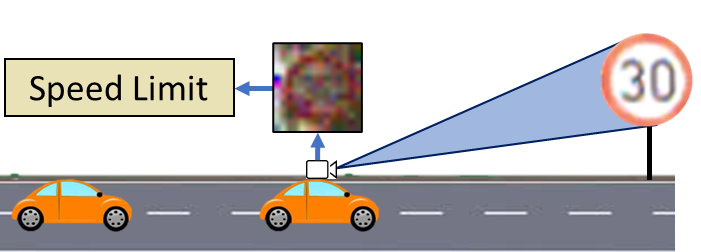
(a) The case when the belief output is correct and there is no accident.

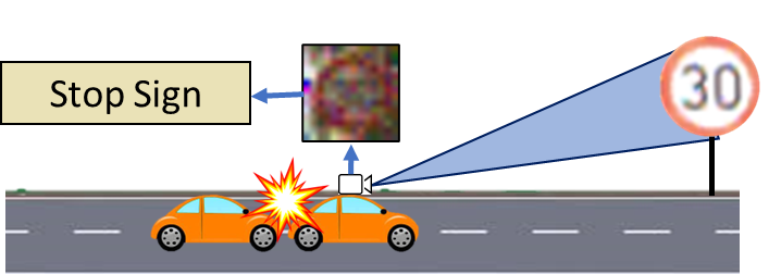
(b) The case when misperception occurs and its corresponding accident.

Figure 1: The above diagram depicts the possible outcomes of the misperception.

The risk quantification process begins with estimating statistics of the belief outputs with a Dirichlet distribution and using the concept of the Voronoi partitioning of the belief space [20] to obtain the discrete distribution of the noisy belief output into class labels. Then, based on the user-defined cost metric for misperceiving each traffic sign, our main result evaluates the risk of traffic sign misperception regarding the severity of the potential accidents.

Our distinct contributions with respect to the existing literature are multi-fold. First, owing to the coherence property, we adopt the Conditional Value-at-Risk (CVaR) measure and propose a risk quantification framework that evaluates the chances of misperception for a given noisy belief output. Secondly, the proposed framework can be customized with a user-defined cost metric and applied to most classification problems when the belief output statistics are available. Thirdly, the proposed approach is control agnostic; given the traffic sign label corresponding to the minimum risk value, our risk-quantification framework is amenable to any control approach. Finally, the case studies demonstrate a significantly improved performance in terms of safety when using the misperception risk to make decisions under varying levels of noise and resolution.

II Mathematical Notations

The $n$-dimensional Euclidean space with elements $\bm{z}=[z_{1},\dots,z_{n}]^{T}$ is denoted by $\mathbb{R}^{n}$, and $\mathbb{R}_{+}$ will denote the positive orthant of $\mathbb{R}$. The collection of all integers is denoted by $\mathbb{Z}$, where $\mathbb{Z}_{+}$ will denote the positive orthant of $\mathbb{Z}$. We represent the $n\times n$ identity matrix as $\bm{I}_{n}$ and the vector of all ones as $\bm{1}_{n}$, respectively. The dimension of a vector $\bm{z}\in\mathbb{R}^{n}$ is shown by $\dim(\bm{z})=n$. The $i$’th element of a vector $\bm{x}$ is shown by $x_{i}$, and when the vector is time indexed by $t$, the notation is adapted to $x_{t,i}$. The $(i,j)$’th entry of matrix $\bm{A}$ is represented by $A_{ij}$. Let us define the collection of all feasible belief vectors $\pi$, i.e., the belief space, as $\mathcal{P}_{n}=\{\pi\in\mathbb{R}_{+}^{n}~{}|~{}\pi^{T}\bm{1}_{n}=1\}$. We also define the Gamma function as $\Gamma(z)=\int_{0}^{\infty}x^{z-1}e^{-x}dx$ for $\mathbf{Re}(z)>0$, and the corresponding Digamma function as $\Psi(x)=\frac{\Gamma^{\prime}(x)}{\Gamma(x)}$.

III Problem Statement

In this paper, we tackle risk evaluation associated with (mis)perception of objects while an autonomous agent is in motion to perform its mission. Objects are semantically linked, and the agent’s detection performance depends on its proximity to them.

For the remainder of the paper, let us consider the case of an autonomous vehicle equipped with an onboard camera traveling along a road with traffic signs with labels from $\mathcal{M}=\{1,\ldots,m\}$. The car travels at a constant velocity towards a traffic sign that it will reach in $T\in\mathbb{R}_{+}$ time. Within the time interval $[0,T]$, the car must take a high-level action from a given set $\Lambda$ to ensure conformance to traffic rules [6] based on a finite set of observations ${\bm{y}}_{t}$, $t\in[0,T]$, that, ideally, matches the ground truth sign label $\ell\in\mathcal{M}$. The observations ${\bm{y}}_{t}\in\mathbb{R}^{i_{d}}$ represent images $i_{d}=q_{1}\times q_{2}$ from the onboard camera in vector form.

We model the detection process as a belief-valued function $h(\cdot)$ over the traffic labels $\mathcal{M}$. Formally, we have ${\bm{p}}_{t}=h({\bm{y}}_{t}),$ where the belief output ${\bm{p}}_{t}\in\mathcal{P}_{m}$ is the output of the detection algorithm (see §V-A). The perception output is the value of function $\arg\max\{{\bm{p}}_{t}\}\in\mathcal{M}$ for a given belief output ${\bm{p}}_{t}\in\mathcal{P}_{m}$. The functionality of $\arg\max$ can be interpreted as one of the simplest forms of inference in the context of this work.

In most real-world scenarios, the onboard cameras suffer from limited sensing range, resolutions, and noisy visual input. As a result, the generated belief output can be potentially inaccurate and pertaining to noise. The observation model of the image ${\bm{y}}_{t}\in\mathbb{R}^{i_{d}}$ is given by

$${\bm{y}}_{t}=g(t,\bm{y}_{0})+b_{t}\,\bm{\xi}_{t},$$ (1)

where $\bm{y}_{0}\in\mathbb{R}^{i_{d}}$ denotes the high resolution and noise-free image of the traffic sign. These types of perturbation are commonly considered in the research of adversarial attacks of the image classification process using neural network models, see [5, 9, 32].

The nonlinear function $g:[0,T]\times\mathbb{R}^{i_{d}}\rightarrow\mathbb{R}^{i_{d}}$ modifies the image $\bm{y}_{0}$ with various resolutions together with the exogenous disturbances $\bm{\xi}_{t}$, which denotes the vector of pixel-wise independent Brownian motions with a time-varying diffusion coefficient $b_{t}$. The detail of this modification is further illustrated in §VII-B.

Definition 1.

For a given belief output ${\bm{p}}_{t}\in\mathcal{P}_{m}$, a misperception occurs if

$$\arg\max\{{\bm{p}}_{t}\}\neq\ell,$$ (2)

where $\ell\in\mathcal{M}$ is the ground truth label of the sign.

The problem is to quantify the risk of misperception as a function of the statistics of the noisy belief output ${\bm{p}}_{t}$ and the given confidence level. To reveal the severity of the misperception, we incorporate the user-defined cost metric with the CVaR measure, which connects the event of misperception with the potential loss due to accidents. Once the risk is assessed, the perceived outcome, which corresponds to a traffic sign with the minimal risk level, can be used with any controller of choice, e.g., low-level controller, symbolic controller, or both [19, 16, 28].

IV Preliminaries

For the exposition of our main result, let us first introduce some necessary results and definitions.

IV-A The Voronoi Partition of the Belief Space

All possible belief outputs ${\bm{p}}_{t}$ belong to the belief space $\mathcal{P}_{m}$, which is a $(m-1)-$simplex in $\mathbb{R}^{m}$. The perception model decides the label of the class is $i\in\mathcal{M}$ if and only if $p_{t,i}>p_{t,j}$ for all $j\in\mathcal{M}$ and $j\neq i$. The $\arg\max$ classification criterion can be explicitly represented via the Voronoi partitioning [17]. The Voronoi partitions of the belief space $\mathcal{P}_{m}$ are given by $V_{1},V_{2},\dots,V_{m}$, where

$$V_{i}=\left\{{\bm{p}}_{t}\in\mathcal{P}_{m}~{}|~{}p_{t,i}>p_{t,j},~{}\forall j\neq i\right\}.$$ (3)

The above partitioning is equivalent to the $\arg\max$ criterion since $\arg\max\{{\bm{p}}_{t}\}=i$ if and only if ${\bm{p}}_{t}\in V_{i}$, see [20].

IV-B Conditional Value-at-Risk Measure

To quantify the uncertainty level and the expected outcome encapsulated in belief outputs, we employ the notion of Conditional Value-at-Risk (CVaR) measure [25]. The CVaR indicates the severity of a random variable landing inside an undesirable set of values that characterizes the dangerous state of the system operation with specific confidence level, i.e., Value-at-Risk (VaR). In probability space $(\Omega,\mathcal{F},\mathbb{P})$, the VaR of the random variable $Y:\Omega\rightarrow\mathbb{R}$ is defined as

$$\mathcal{R}^{\varepsilon}_{VaR}(Y)=\min\{z\mid F_{Y}(z)\geq 1-\varepsilon\},$$ (4)

where the cumulative distribution function $F_{Y}(z)=\mathbb{P}\{Y\leq z\}$. Then, the CVaR is defined as follows.

Definition 2.

The Conditional-Value-at-Risk with the confidence level $(1-\varepsilon)\in[0,1]$ is the mean of the generalized $\varepsilon-$tail distribution:

$$\mathcal{R}^{\varepsilon}_{CVaR}(Y)=\int_{-\infty}^{\infty}z~{}dF_{Y}^{\varepsilon}(z),$$ (5)

where

$$F_{Y}^{\varepsilon}(z)=\begin{cases}0,\hskip 66.86414pt\text{if }z<\mathcal{R}^{\varepsilon}_{VaR}(Y)\\ \frac{F_{Y}(z)+\varepsilon-1}{\varepsilon},\hskip 28.45274pt\text{if }z\geq\mathcal{R}^{\varepsilon}_{VaR}(Y)\end{cases}.$$ (6)

A smaller value of $\varepsilon$ indicates a higher level of confidence on random variable $Y$ to stay below $\mathcal{R}^{\varepsilon}_{VaR}(Y)$. If $Y$ has a continuous distribution function, CVaR can be obtained as the conditional expectation of $Y$ subject to $Y\geq\mathcal{R}^{\varepsilon}_{VaR}(Y)$. In the case of discrete distributions, one may need to split a probability atom, and CVaR may be obtained by averaging a fractional number of scenarios, see [27].

V Traffic Sign Perception Model

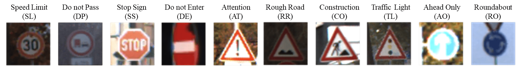
Figure 2: Ten traffic signs selected from the GTSRB dataset.

In this paper, we assume that an off-the-shelf detection algorithm for sign detection is available, e.g., [14, 37, 34], and it can be used to obtain a guess of the sign’s ground truth label $\ell$ at every time $t\in[0,T]$. For simplicity, we assume that input images contain only the signs cropped from the camera’s image. Example images of the traffic signs are presented in Fig. 2. We use the German Traffic Sign Recognition Benchmark (GTSRB) dataset to simulate the perception of the vehicle while driving toward the traffic sign. We modify the images from the GTSRB dataset with time-varying resolution and pixel-wise noise, such that the observed image ${\bm{y}}_{t}$ is a random variable. Examples of the modification are presented in §VII-B.

V-A Perception Model

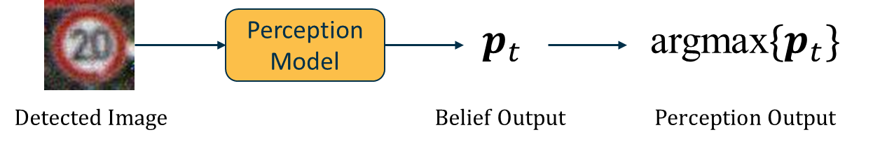
Figure 3: The traffic sign perception process.

The noisy observation ${\bm{y}}_{t}$ is fed into the perception model as an image. In this paper, we consider the perception model as a simple convolutional neural network (CNN) model, e.g., VGG-19 [29], such that ${\bm{p}}_{t}=h({\bm{y}}_{t})$ can be rewritten as

$${\bm{p}}_{t}=\texttt{Softmax}\left(\,\text{CNN}({\bm{y}}_{t})\,\right),$$ (7)

in which belief outputs $\bm{p}_{t}=(p_{t,1},\cdots,p_{t,m})\in\mathcal{P}_{m}$ are generated for all continuous time instances within $[0,T]$, as depicted in Fig. 3.

The focus of this work is not to improve the accuracy of detection/recognition algorithms but rather to integrate them with risk quantification to further strengthen the perception module against misperception by reasoning about the severity of the potential failure. For clarity, we choose a simple detection model. However, with simple modifications, the proposed approach applies to any detection model [13, 36].

V-B Estimated Statistics of Belief Outputs

To quantify the risk, one must obtain or estimate the statistics of the target random variable. Measuring the statistics of belief output ${\bm{p}}_{t}$ for the entire time-span $[0,T]$ is inefficient due to the time-varying resolution and noise in (1). To resolve this issue, we assume that the statistics of ${\bm{p}}_{t}$ do not change drastically in any sufficiently short time interval $[t-\tau,t)\subset[0,T]$, $\tau\in\mathbb{R}_{+}$ and $t\in[\tau,T]$, and we can only obtain a finite number of observations in each time interval. Let $\mathcal{T}_{t}^{\tau}\subset[0,T]$ be the finite set of (uniform or non-uniform) sampling times, and $q=|\mathcal{T}_{t}^{\tau}|$, the cardinality of the set $\mathcal{T}_{t}^{\tau}$. Even for the interval $[t-\tau,t)$, quantifying the statistics of ${\bm{p}}_{t}$ from the $q$ observations is not intuitive since the random variable follows the constraint

$$\sum_{i}p_{t,i}=1\text{ and }p_{t,i}\geq 0\text{ for all $i\in\mathcal{M}$},$$ (8)

which falls within the belief space $\mathcal{P}_{m}$. Unlike well-known distribution fitting approaches for Gaussian random variables, we estimate the statistics of ${\bm{p}}_{t}$ using a Dirichlet distribution, for which the corresponding random variable satisfies (8). A random variable $\bm{z}\in\mathcal{P}_{m}$ with the Dirichlet distribution $\mathcal{D}(\bm{z},\bm{\alpha})$ has probability density function

$$f_{\mathcal{D}}(z_{1},...,z_{m};\alpha_{1},...,\alpha_{m})=\frac{\Gamma(\sum_{i=1}^{m}\alpha_{i})}{\prod_{i=1}^{m}\Gamma(\alpha_{i})}\prod_{i=1}^{m}z_{i}^{\alpha_{i}-1},$$ (9)

where $\Gamma(\cdot)$ denotes the Gamma function, $\sum_{i\in\mathcal{M}}z_{i}=1$, and $z_{i}\geq 0$ for all $i\in\mathcal{M}$, and $\bm{\alpha}\in\mathbb{R}^{m}_{+}$ is the concentration parameter vector of the $m$-order Dirichlet distribution.

Let us consider $q$ images, sampled and processed over a time interval $[t-\tau,t)$, and their corresponding collection of belief outputs is given as a $q\times m$ matrix $\bm{P}_{t}=[\bm{p}_{t^{\prime}}^{T}]_{t^{\prime}\in\mathcal{T}^{\tau}_{t}}.$ We use the fixed point approach proposed in [22] to estimate the Dirichlet distribution, i.e., the concentration vector $\bm{\alpha}_{t}$, from a given set of belief outputs $\bm{P}_{t}$. The method maximizes the log-likelihood of the estimated distribution and the original data. Considering the convex nature of the problem [26], the likelihood is unimodal, and its maximum can be obtained via a simple search [22].

Given an initial guess $\hat{\bm{\alpha}}_{t}$ of $\bm{\alpha}_{t}$, the estimated value of $\bm{\alpha}_{t}$ is updated using the following result.

Lemma 1.

For a given set of belief outputs $\bm{P}_{t}$, there exists a set of values of $\bm{\alpha}_{t}$ which maximizes the log-likelihood, and $\bm{\alpha}_{t}$ can be updated element-wise using

$$\Psi(\alpha_{t,i}^{new})=\Psi(\sum_{j=1}^{m}\alpha_{t,j}^{old})+\frac{1}{q}\sum_{t^{\prime}\in\mathcal{T}^{\tau}_{t}}\log p_{t^{\prime},i},$$ (10)

where $\Psi(\cdot)$ is the Digamma function, $\bm{\alpha}_{t}=(\alpha_{t,1},...,\alpha_{t,m})$, and $i\in\mathcal{M}$.

The proof of the above result is omitted, and it can be obtained from [22]. The above lemma provides the opportunity of estimating the statistics of belief outputs ${\bm{p}}_{t}$ for the time interval $[t-\tau,t)$ with a Dirichlet random variable ${\bm{z}}_{t}\sim\mathcal{D}({\bm{z}}_{t},\bm{\alpha}_{t})$, which allows us to compute the risk of misperception in a closed form.

VI Risk of Misperception

We introduce the cost for misperceiving traffic signs followed by our main result of misperception risk.

VI-A Cost of Traffic Signs Misperception

Sign	SL	DP	SS	DE	AT	RR	CO	TL	AO	RO
SL	0	174	103	103	123	123	121	103	121	120
DP	117	0	105	105	117	117	119	105	97	113
SS	135	109	0	96	110	110	110	96	135	135
DE	117	117	99.5	0	117	500	117	117	117	117
AT	71	111.5	102	92	0	50	0	102	51	137.5
RR	144.5	168	82	82	50	0	50	140	168	258
CO	102	41.5	82	82	30	0	0	41	83	173
TL	97	97	77.5	77.5	39	73	73	0	73	163
AO	91	91	86.5	86.5	45.5	45.5	45.5	91	0	182
RO	83	83	165	165	41.5	41.5	41.5	63	200	0

TABLE I: The cost metric for traffic sign misperception (unit: $\text{\texteuro}1000$).

Misperceiving traffic signs often leads to poor decisions of autonomous vehicles, which are primarily associated with high potential costs in real-world driving scenarios. Simply interpreting the belief output as “correct” or “wrong” does not provide adequate information for safe autonomous driving. The reason is that the high-level actions associated with each traffic sign do not yield the same potential cost, e.g., misperceiving the “Speed-limit” sign as a “Stop” sign induces a higher cost than misperceiving it as a “Construction” sign.

Therefore, to explore the severity of the misperception that is beyond correctness, we introduce a cost matrix of misperceiving the traffic signs, $C\in\mathbb{R}^{m\times m}$. For each label $i\in\mathcal{M}$, we define the cost of misperceiving the label $j\in\mathcal{M}$ as the label $i$ as $C_{ji}$. The correct perception incurs zero cost, i.e., $C_{jj}=0$. The cost value is user-specific, in this paper, we used the cost metric shown in Table I, obtained by merging the estimated cost for the traffic sign-related violations [2] for our selected traffic signs, such as potential fines and vehicle damages.

VI-B Risk of Misperceiving Traffic Signs

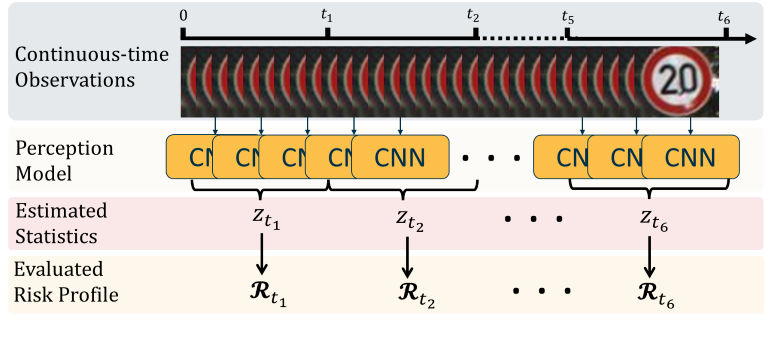
Figure 4: The above figure illustrates the evaluation of the risk profile for each short time interval, using $6$ time intervals as an example.

The cost metric establishes the connection between the estimated belief output ${\bm{z}}_{t}$ to the potential cost of misperception given by the cost metric. For each traffic sign, there exist $m-1$ possible cases that the estimated perception output $\arg\max\{{\bm{z}}_{t}\}$ is incorrect. For a given estimated belief output ${\bm{z}}_{t}$, one can deterministically define a family of nonlinear functions $r_{i}(\cdot)|_{i\in\mathcal{M}}$ that maps ${\bm{z}}_{t}$ into the cost metric of misperceptions. For label $i$, the function $r_{i}(\cdot)$ takes value in $C_{ji}|_{j\in\mathcal{M}}$ such that

$$r_{i}({\bm{z}}_{t})=C_{ji}\text{ if }{\bm{z}}_{t}\in V_{j}.$$ (11)

Then, the risk quantification can be adjusted to a family of discrete random variables, $r_{i}({\bm{z}}_{t})$ for $i\in\mathcal{M}$.

Given the fact that one or more instances of misperception may obtain the same cost value, let us denote the ordered cost vector as $\bm{c}_{i}\in\mathbb{R}^{m^{\prime}_{i}}$, where the integer $m^{\prime}_{i}\leq m$. The value of $m^{\prime}_{i}$ denotes the number of unique values in all $C_{ji}|_{j\in\mathcal{M}}$, and the element of $\bm{c}_{i}$ obtains the unique values of $C_{ji}$ in a descending order such that

$$\max_{j\in\mathcal{M}}C_{ji}=(\bm{c}_{i})_{1}>\cdots>(\bm{c}_{i})_{m^{\prime}_{i}}=\min_{j\in\mathcal{M}}C_{ji}.$$

For the $i$’th label, there exist $m^{\prime}_{i}$ possible cost values for $r_{i}({\bm{z}}_{t})$. Then, the corresponding discrete probability distribution of $r_{i}({\bm{z}}_{t})$ can be computed as follows.

Lemma 2.

For each element of ordered cost vector $\bm{c}_{i}$, the probability of $\mathbb{P}\{r_{i}({\bm{z}}_{t})=(\bm{c}_{i})_{j}\}$ is given by

$$\mathbb{P}\{r_{i}({\bm{z}}_{t})=(\bm{c}_{i})_{j}\}=\hat{p}_{t,j}=\sum_{k|C_{k,i}=(\bm{c}_{i})_{j}}\mathbb{P}\{{\bm{z}}_{t}\in V_{k}\},$$ (12)

where

$$\mathbb{P}\{{\bm{z}}_{t}\in V_{k}\}=\int_{0}^{\infty}\prod_{i\neq k}\left(\frac{\gamma(\alpha_{t,i},x)}{\Gamma(\alpha_{t,i})}\right)\frac{x^{\alpha_{t,k}-1}\exp{(-x)}}{\Gamma(\alpha_{t,k})}dx,$$ (13)

and $\gamma(\alpha,x)$ is the lower incomplete gamma function.

The integral in (13) can be obtained numerically using the approach proposed in [31] for computing the exceedance probability in the Dirichlet distribution. With the knowledge of the ordered cost vector $\bm{c}_{i}|_{i\in\mathcal{M}}$, the estimated statistics of belief outputs ${\bm{z}}_{t}$, and its corresponding cost output $r_{i}({\bm{z}}_{t})$, the Conditional Value-at-Risk of traffic sign misperception is shown in the following result.

Theorem 1.

During the time interval $[t-\tau,t)$, given the estimated belief output ${\bm{z}}_{t}$, the risk of misperception with the $i$’th label is given by

$$\mathcal{R}_{t,i}^{\varepsilon}=\frac{1}{\varepsilon}\left(\sum_{j=1}^{v}(\bm{c}_{i})_{j}\,\hat{p}_{t,j}+(\bm{c}_{i})_{v+1}\big{(}\varepsilon-\sum_{j=1}^{v}\hat{p}_{t,j}\big{)}\right),$$ (14)

where the value of $v\in\mathbb{Z}$ is computed by

$$v=\sup_{v\leq m^{\prime}_{i}}~{}\sum_{j=1}^{v}\hat{p}_{t,j}\leq\varepsilon,$$ (15)

the value of $\hat{p}_{t,j}$ is obtained from (12), and the value of $1-\varepsilon$ represents the confidence level.

The above theorem provides the closed-form representation of the risk of misperception when the statistics of the belief output have a Dirichlet distribution. For a given confidence level $1-\varepsilon$, the magnitude of $\mathcal{R}^{\varepsilon}_{t,i}$ quantifies the severity of potential loss when perceiving the traffic sign as the $i$’th label based on the statistics of ${\bm{z}}_{t}$.

At each discrete time step $t$, let us also denote the collection of misperception risks for every label as the risk profile of misperception, such that

$$\bm{\mathcal{R}}_{t}^{\varepsilon}=[\mathcal{R}_{t,1}^{\varepsilon},\mathcal{R}_{t,2}^{\varepsilon},\cdots,\mathcal{R}_{t,m}^{\varepsilon}]^{T}\in\mathbb{R}^{m},$$ (16)

and the risk evaluation process is depicted in Fig. 4. The risk output is again a label obtained via the $\arg\min$ rule, i.e., $\arg\min\{\bm{\mathcal{R}}_{t}^{\varepsilon}\}\in\mathcal{M}$.

VI-C Accumulated Risk

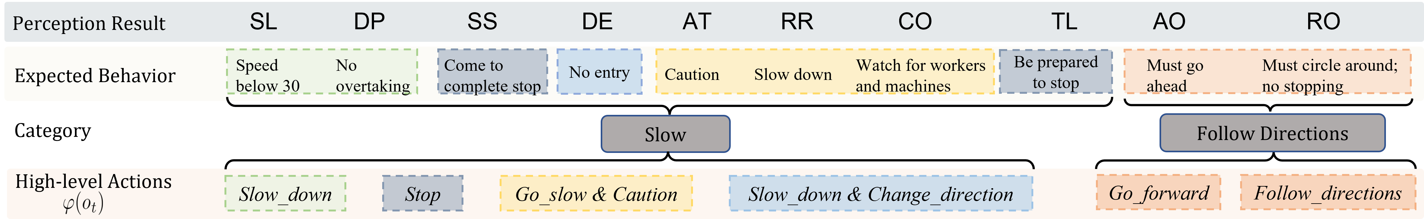
Figure 5: The high-level actions to be executed upon encountering a specific traffic sign.

The risk of misperception is capable of assessing the reliability of the belief output for a time interval $[t-\tau,t)$. However, in the real-world environment, the input quality is time-varying, and simply relying on the risk output for one short time does not reveal the truth about the target traffic sign. Thus, it also requires us to track the change of the risk throughout time and consider both current and past information. To this end, consider a weighted average of risk values with a scaling factor $\mu\in(0,1)$ which balances the importance of the present and the past risk values

$$\hat{\mathcal{R}}_{t,i}^{\varepsilon}=\frac{1-\mu}{1-\mu^{K}}\sum_{k=1}^{K}\mu^{K-k}\,\mathcal{R}_{k\tau,i}^{\varepsilon},$$ (17)

where $t=K\cdot\tau$ is the current time at step $K\in\mathbb{Z}_{+}$, $\mathcal{R}^{\varepsilon}_{k\tau,i}$ is evaluated at each time $t^{\prime}=k\tau$ of step $k\in\{1,\ldots,K\}$ using (14), and $\mu\in(0,1)$ is the user-specified scaling factor. The corresponding risk profile can be stacked as $\bm{\hat{\mathcal{R}}}_{t}^{\varepsilon}$ using the same lines of argument in (16).

The accumulated risk shows an evident advantage over the real-time risk $\mathcal{R}_{t,i}$ since it is more inclusive. Moreover, it can handle the situation when the observation changes drastically and the recent observations are unreliable since it does not solely rely on the most recent visual input. The accumulated risk is also normalized to enable tracking of the changes in the risk of misperception, i.e., $\sum_{k=1}^{K}\mu^{K-k}=(1-\mu^{K})/(1-\mu)$

Let us also introduce the critical risk threshold $\eta\in\mathbb{R}_{+}$ as the user-defined maximum acceptable cost of the system. It can be appropriately designed by carefully considering the task and the environmental factors. Once the accumulated risk value $\hat{\mathcal{R}}_{t,i}^{\varepsilon}$ becomes lower than $\eta$, the corresponding accumulated risk output $o_{t}\in\mathcal{M}$ is considered as the label, i.e., it is the minimal element in the risk profile such that

$$o_{t}={\arg\min}_{i\in\mathcal{M}}\{\hat{\bm{\mathcal{R}}}_{t}^{\varepsilon}\},\text{ and }\hat{\mathcal{R}}_{t,o_{t}}^{\varepsilon}\leq\eta.$$ (18)

VII Case Study

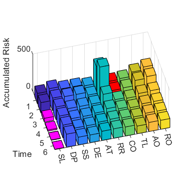
(a) True label: Speed-limit (SL)
$\varphi(SL)=$Slow_down

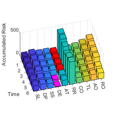
(b) True label: Do not enter (DE)
$\varphi(DE)=$Slow_down & Change_direction

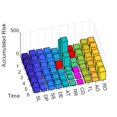
(c) True label: Construction (CO)
$\varphi(CO)=$Go_slow & Caution

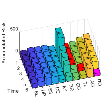
(d) True label: Roundabout (RO)
$\varphi(RO)=$Follow_directions

Figure 6: The accumulated risk profile of misperception for various traffic signs $\bm{\hat{\mathcal{R}}}_{t}^{\varepsilon}$. At each time step, the label corresponding to minimum risk is shown in red, and the bar indicating $o_{t}$ is shown in magenta.

In this case study, the perception model is trained with the original GTSRB dataset, and the risk of misperception is evaluated with the modified image. Let us consider $\tau=\frac{T}{6}$ and split $[0,T]$ in to $6$ intervals for all case studies. We now define some notions used for evaluating the proposed risk metric and then proceed with a detailed discussion on simulations.

VII-A High-Level Actions and Time To Execution

We consider a set $\Lambda$ of prescribed high-level actions that allow the system to execute an appropriate maneuver corresponding to the detected sign as depicted in Fig. 5. The high-level actions are the abstractions of actuation commands to the system.

Given the accumulated risk output $o_{t}$, $\varphi:\mathcal{M}\rightarrow\Lambda$ provides an action $\lambda\in\Lambda$ to be executed. In order to facilitate the execution of the chosen high-level actions, our framework maximizes the time to execution ($t_{exec}$) defined as follows:

$$t_{exec}=(T-t)\cdot I(\hat{\bm{\mathcal{R}}}_{t}^{\varepsilon}\leq\eta),$$ (19)

where $I(\cdot)$ is an indicator function and takes the value 1 whenever $\hat{\bm{\mathcal{R}}}_{t}^{\varepsilon}$ drops below the risk threshold $\eta$ and is 0 otherwise. Thus, once the normalized accumulated risk crosses the acceptable cost $\eta$, a corresponding high-level action can be chosen.

As this work focuses on strengthening perception-related safety using risk quantification, we consider a simple mapping between the accumulated risk output $o_{t}$ to the action space $\Lambda$. Developing risk-aware controllers is a topic for future investigation.

VII-B Modified GTSRB Dataset

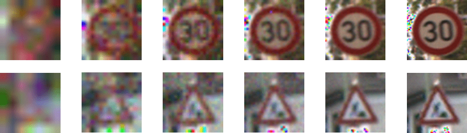
Figure 7: Example images from the modified GTSRB dataset. Shown for $6$ time intervals.

Since the images from the GTSRB dataset are static and do not contain any specific types of noise, we apply the following modifications to the dataset, which simulates the scenarios of the vehicle approaching the traffic sign:

• The quality of the detected image is time-varying. The resolution of the detected images increases when the vehicle gets closer to the traffic sign, i.e., as $t$ increases.

• The independent time-varying Gaussian noise is added to each pixel of the image. The magnitude of the noise, $b_{t}$, decreases as the vehicle gets closer to the traffic sign, i.e., as $t$ increases.

We select $10$ types of traffic signs from the dataset, and examples of the modified image are shown in Fig. 7. The above modification can be represented using (1), in which we consider $g(\cdot)$ is the function that changes the resolution w.r.t the time $t$, and $b_{t}$ is the time-varying noise magnitude. For instance, our choices are $\dim(g(t,\bm{y}_{0}))=\frac{t}{T}\dim(\bm{y}_{0})$ and $b_{t}=0.02\frac{T}{t}$.

VII-C Simulations

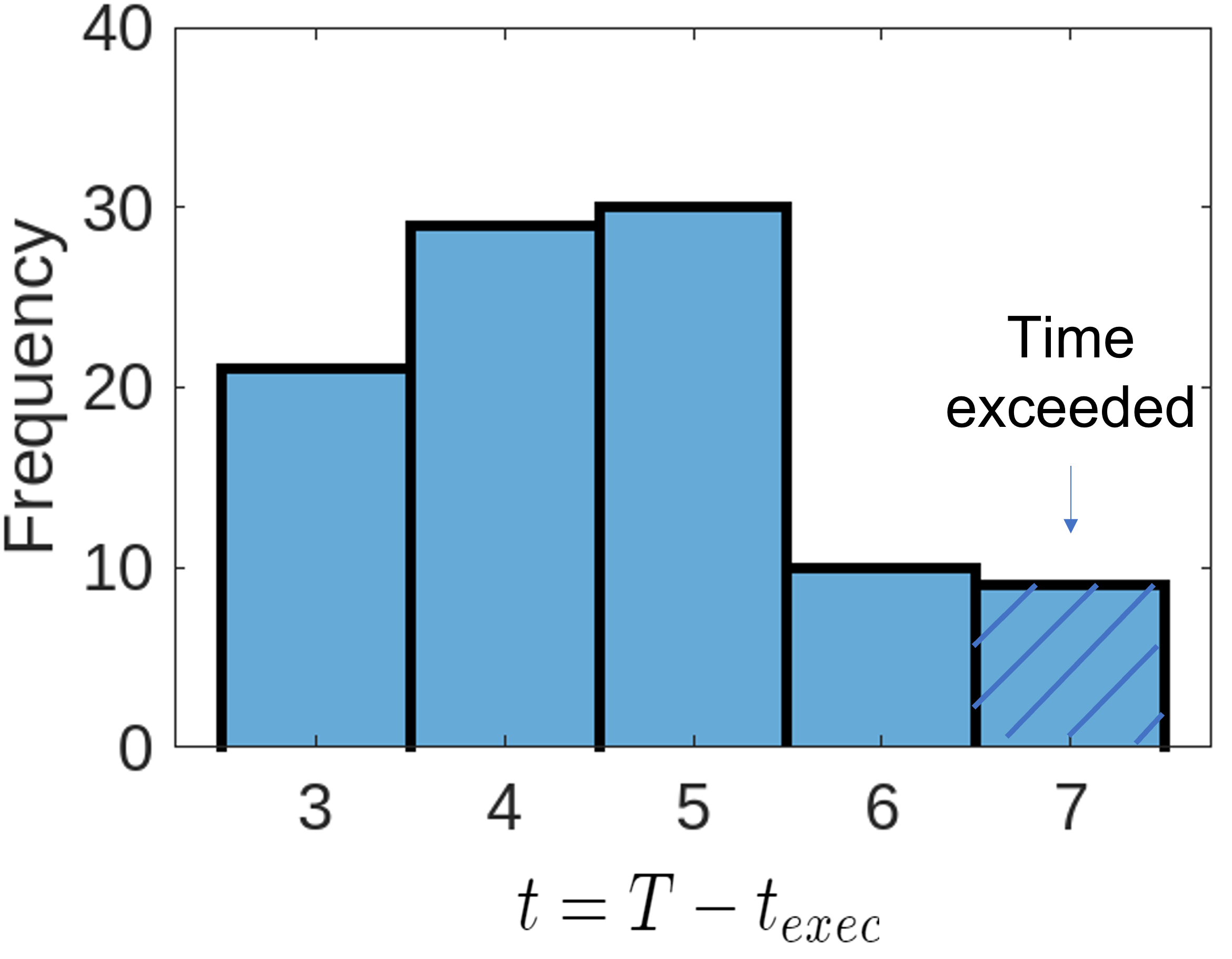
(a) $\eta=\text{\texteuro}1000$.

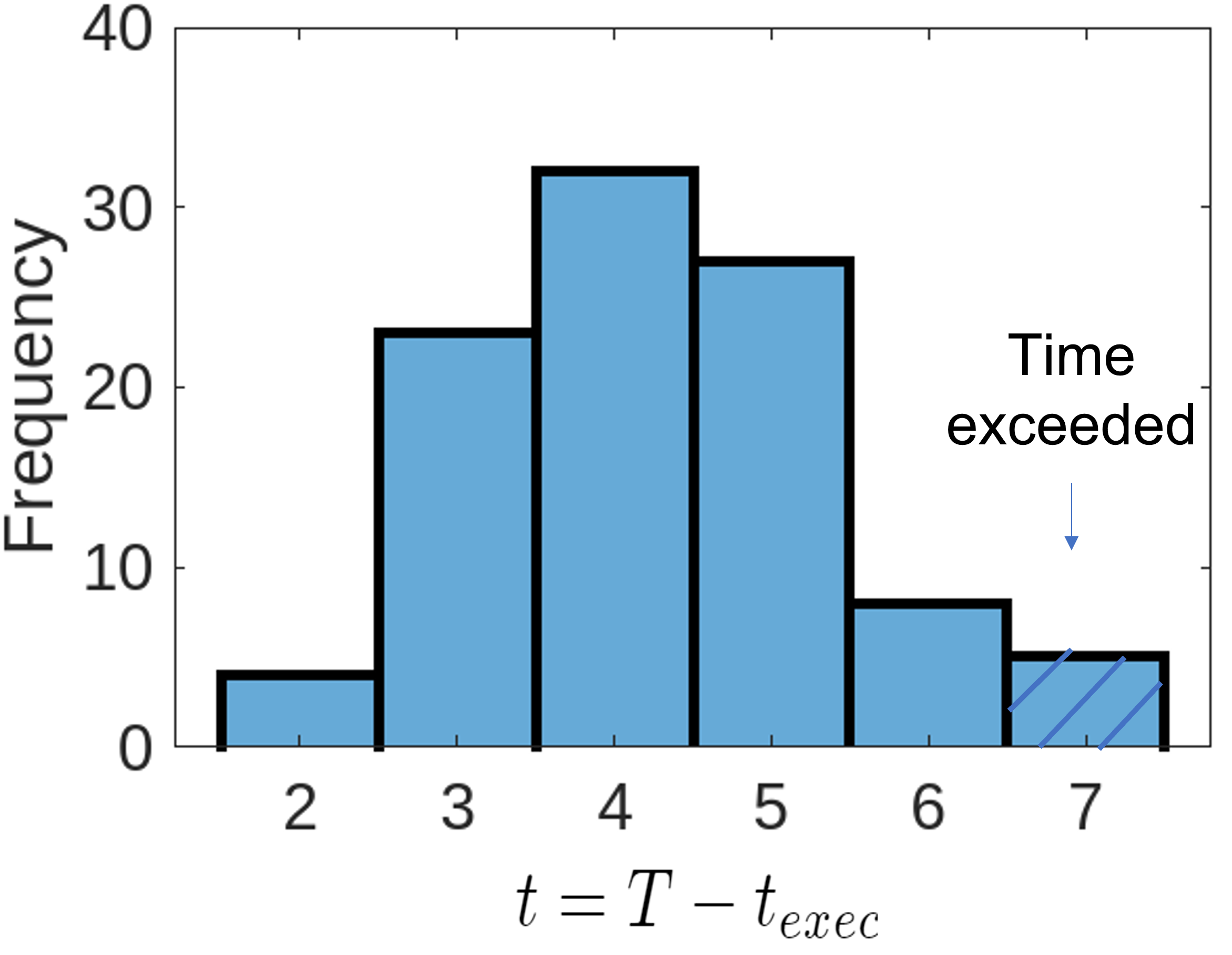
(b) $\eta=\text{\texteuro}10000$.

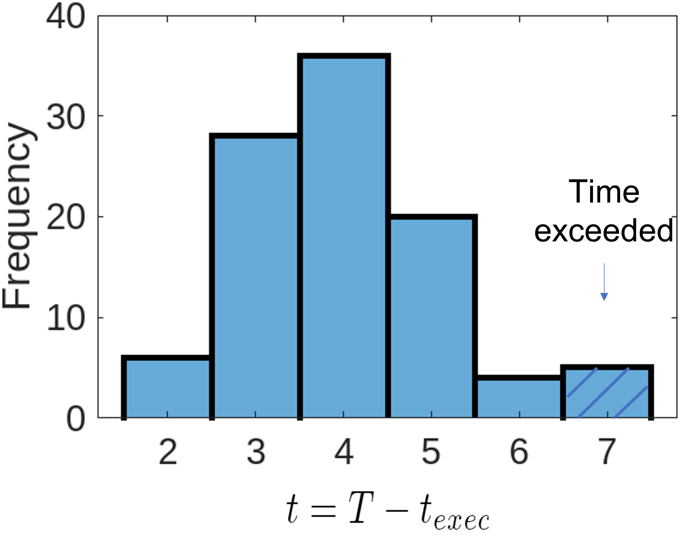
(c) $\eta=\text{\texteuro}50000$.

Figure 8: The distribution of $T-t_{exec}$ with various $\eta$. Evaluated among $100$ trails.

VII-C1 Risk of Traffic Sign Misperception

Using the result from Theorem 1, we evaluate the risk of misperceiving specific signs, for which some examples are shown in Fig. 6. The tested images are taken from the modified GTSRB dataset with $\eta=\text{\texteuro}10000$ and the confidence level is set by letting $\varepsilon=0.1$. Among all presented cases, the ground truth labels of the sign $\ell\in\mathcal{M}$ are associated with the accumulated risk output $o_{t}$ by $t=6$.

There are a few interesting observations that are worth reporting: The label ${\arg\min}_{i\in\mathcal{M}}\{\bm{\hat{\mathcal{R}}}_{t}^{\varepsilon}\}$ commonly occurs at “CO” when the input image is noisy and with low resolution. This phenomena is because the action related to “CO” is “Go_slow & Caution” (see Fig. 5), which is intuitively the safest action when the visual input is not reliable. The severity of different instances of misperceptions depends on the expected high-level actions to be executed, e.g., in Fig. 6(c), the high-level actions associated with “AT”, “RR”, and “CO” are the same, and thus, their corresponding accumulated risks lie within the same range of values. Therefore, the system will not incur a penalty even in case of misperception. In Fig. 6(d), the risk output $o_{t}$ is only obtained at $t=6$, since the potential loss of misperceiving the label “RO” is relatively high, and the decision should only be made when the visual input is reliable enough, i.e., $\hat{\mathcal{R}}_{t,o_{t}}^{\varepsilon}\leq\eta$.

VII-C2 Critical Risk Threshold

Given different values of the critical risk threshold $\eta$, it is expected to observe various distributions of the time to execution $t_{exec}$, which is presented in Fig. 8. The result indicates that with the increase of the threshold $\eta$, the autonomous vehicle could make earlier decisions owing to the higher acceptable potential cost. Thus, the distribution of $t_{exec}$ is more concentrated in higher values, or the distribution of $T-t_{exec}$ is more concentrated toward lower values. Our result also reveals a potential trade-off between $\eta$ and $t_{exec}$ as a smaller choice of $\eta$ may prevent autonomous vehicles from making early decisions.

VII-C3 Risk Outputs vs Perception Outputs

The risk output ${\arg\min}_{i\in\mathcal{M}}\{\bm{\mathcal{R}}_{t}^{\varepsilon}\}$ exhibits a significant advantage compared to the perception output $\arg\max\{{\bm{p}}_{t}\}$ in the view of preventing the potential losses. We compare the ratio of correct high-level actions, i.e., the action accuracy, generated with both approaches with various noise and resolution levels, as shown in Fig. 9. In both cases, the risk output ${\arg\min}_{i\in\mathcal{M}}\{\bm{\mathcal{R}}_{t}^{\varepsilon}\}$ outperforms the perception output $\arg\max\{{\bm{p}}_{t}\}$ by nearly $20\%$ in the action accuracy. It is because the consequences of each high-level action are inclusively considered in the risk of misperception, which exhibits the major difference between these two approaches.

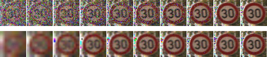
(a) Example images with: 1) Fixed relative resolution ($100\%$) with various noise levels; 2) Fixed noise level $b_{t}=0.04$ with various resolution levels;

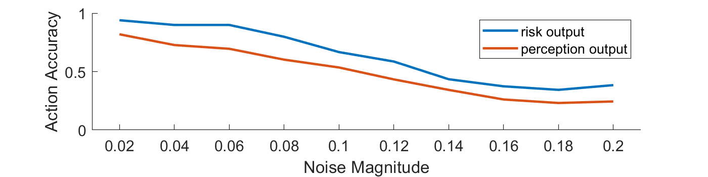
(b) Action Accuracy vs Noise.

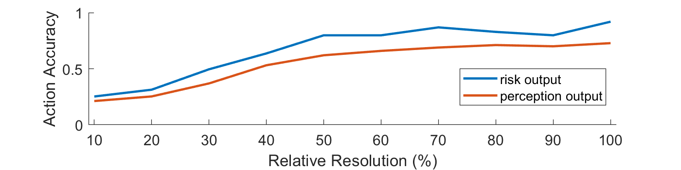
(c) Action Accuracy vs Resolution.

Figure 9: Action accuracy with various noise levels and resolutions.

VIII Conclusion

In this work, we address the problem of mitigating the effects of misperceiving traffic signs for autonomous driving given noisy visual input. Using the well-known CVaR measure, we construct the framework that evaluates the risk of misperception as a function of the estimated belief output statistics and the user-specified cost metric that captures the severity of potential failures to the system in the event of misperception. Furthermore, leveraging the gradual improvements in the detection accuracy due to gradually improving sensing resolution and smaller effect of noise, we define a discounted accumulated CVaR-based risk. The proposed risk measure reveals the risk output and the accumulated risk output that can be utilized for decision-making and control with any controller of choice. The extensive case studies demonstrate the effectiveness of the proposed risk-quantification framework.

This work is the first step in incorporating the risk of misperception into the perception-planning framework with a focus on the perception module. The immediate natural extension of the work is to design a risk-aware controller to guarantee desirable properties such as system safety and minimum time execution. It also enables the analysis of the perception model from the view of the misperception risk when the output statistics can be explicitly written as a function of model parameters [1].

References

- [1] Arash Amini, Guangyi Liu and Nader Motee “Robust Learning of Recurrent Neural Networks in Presence of Exogenous Noise” In 2021 60th IEEE Conference on Decision and Control
- [2] Mercedes Ayuso, Montserrat Guillén and Manuela Alcañiz “The impact of traffic violations on the estimated cost of traffic accidents with victims” In Accident Analysis & Prevention 42.2 Elsevier, 2010
- [3] Istvan Barabás, Adrian Todoruţ, N Cordoş and Andreia Molea “Current challenges in autonomous driving” In IOP conference series: materials science and engineering 252.1, 2017, pp. 012096 IOP Publishing
- [4] Fernando S Barbosa, Bruno Lacerda, Paul Duckworth, Jana Tumova and Nick Hawes “Risk-aware motion planning in partially known environments” In 2021 60th IEEE Conference on Decision and Control (CDC), 2021, pp. 5220–5226 IEEE
- [5] Fabio Carrara, Fabrizio Falchi, Giuseppe Amato, Rudy Becarelli and Roberto Caldelli “Detecting Adversarial Inputs by Looking in the black box” In arXiv preprint arXiv:1803.02111, 2018
- [6] “Convention on road traffic of 1968 and European Agreement supplementing the convention” In UNECE URL: https://unece.org/info/Transport/Road-Traffic-and-Road-Safety/pub/2636
- [7] Sarah Dean, Nikolai Matni, Benjamin Recht and Vickie Ye “Robust guarantees for perception-based control” In Learning for Dynamics and Control, 2020, pp. 350–360 PMLR
- [8] Vinayak V Dixit, Sai Chand and Divya J Nair “Autonomous vehicles: disengagements, accidents and reaction times” In PLoS one 11.12 Public Library of Science San Francisco, CA USA, 2016
- [9] Yinpeng Dong, Qi-An Fu, Xiao Yang, Tianyu Pang, Hang Su, Zihao Xiao and Jun Zhu “Benchmarking adversarial robustness on image classification” In proceedings of the IEEE/CVF conference on computer vision and pattern recognition, 2020, pp. 321–331
- [10] Mica R Endsley “Autonomous driving systems: A preliminary naturalistic study of the Tesla Model S” In Journal of Cognitive Engineering and Decision Making 11.3 SAGE Publications Sage CA: Los Angeles, CA, 2017
- [11] Francesca M Favarò, Nazanin Nader, Sky O Eurich, Michelle Tripp and Naresh Varadaraju “Examining accident reports involving autonomous vehicles in California” In PLoS one 12.9 Public Library of Science San Francisco, CA USA, 2017
- [12] Astghik Hakobyan, Gyeong Chan Kim and Insoon Yang “Risk-aware motion planning and control using CVaR-constrained optimization” In IEEE Robotics and Automation letters 4.4 IEEE, 2019
- [13] Mrinal Haloi “Traffic sign classification using deep inception based convolutional networks” In arXiv preprint arXiv:1511.02992, 2015
- [14] Sebastian Houben, Johannes Stallkamp, Jan Salmen, Marc Schlipsing and Christian Igel “Detection of traffic signs in real-world images: The German Traffic Sign Detection Benchmark” In The 2013 international joint conference on neural networks (IJCNN)
- [15] Clemens Markus Hruschka, Daniel Töpfer and Sebastian Zug “Risk assessment for integral safety in automated driving” In 2019 2nd International Conference on Intelligent Autonomous Systems
- [16] Disha Kamale, Sofie Haesaert and Cristian-Ioan Vasile “Cautious Planning with Incremental Symbolic Perception: Designing Verified Reactive Driving Maneuvers” In 2023 IEEE/RSJ International Conference on Robotics and Automation (ICRA)
- [17] R. Klein “Abstract Voronoi diagrams and their applications” In Workshop on Computational Geometry, 1988 Springer
- [18] Xiao Li, Jonathan DeCastro, Cristian Ioan Vasile, Sertac Karaman and Daniela Rus “Learning A Risk-Aware Trajectory Planner From Demonstrations Using Logic Monitor” In Conference on Robot Learning, 2022, pp. 1326–1335 PMLR
- [19] Chang Liu, Seungho Lee, Scott Varnhagen and H Eric Tseng “Path planning for autonomous vehicles using model predictive control” In 2017 IEEE Intelligent Vehicles Symposium (IV)
- [20] Guangyi Liu, Arash Amini, Martin Takac and Nader Motee “Robustness Analysis of Classification Using Recurrent Neural Networks with Perturbed Sequential Input” In arXiv preprint arXiv:2203.05403, 2022
- [21] Anirudha Majumdar and Marco Pavone “How should a robot assess risk? towards an axiomatic theory of risk in robotics” In Robotics Research Springer, 2020, pp. 75–84
- [22] Thomas Minka “Estimating a Dirichlet distribution” Technical report, MIT, 2000
- [23] Gerhard Neuhold, Tobias Ollmann, Samuel Rota Bulo and Peter Kontschieder “The mapillary vistas dataset for semantic understanding of street scenes” In Proceedings of the IEEE international conference on computer vision, 2017, pp. 4990–4999
- [24] R.. Rockafellar and S. Uryasev “Optimization of Conditional Value-at-Risk” In Portfolio The Magazine Of The Fine Arts 2, 1999, pp. 1–26
- [25] R. Rockafellar and Stanislav Uryasev “Conditional value-at-risk for general loss distributions” In Journal of Banking and Finance 26.7, 2002, pp. 1443–1471
- [26] Gerd Ronning “Maximum likelihood estimation of Dirichlet distributions” In Journal of statistical computation and simulation 32.4 Taylor & Francis, 1989, pp. 215–221
- [27] Sergey Sarykalin, Gaia Serraino and Stan Uryasev “Value-at-risk vs. conditional value-at-risk in risk management and optimization” In State-of-the-art decision-making tools in the information-intensive age Informs, 2008, pp. 270–294
- [28] Wilko Schwarting, Javier Alonso-Mora and Daniela Rus “Planning and decision-making for autonomous vehicles” In Annual Review of Control, Robotics, and Autonomous Systems 1 Annual Reviews, 2018, pp. 187–210
- [29] K. Simonyan and A. Zisserman “Very deep convolutional networks for large-scale image recognition” In 3rd International Conference on Learning Representations, 2015
- [30] Santokh Singh “Critical reasons for crashes investigated in the national motor vehicle crash causation survey”, 2015
- [31] Joram Soch and Carsten Allefeld “Exceedance Probabilities for the Dirichlet Distribution” In arXiv:1611.01439, 2016
- [32] Akshayvarun Subramanya, Vipin Pillai and Hamed Pirsiavash “Fooling network interpretation in image classification” In Proceedings of the IEEE/CVF international conference on computer vision, 2019, pp. 2020–2029
- [33] Chuanning Wei, Michael Fauß and Margaret P Chapman “CVaR-based Safety Analysis in the Infinite Time Horizon Setting” In 2022 American Control Conference (ACC), 2022 IEEE
- [34] Yi Yang, Hengliang Luo, Huarong Xu and Fuchao Wu “Towards real-time traffic sign detection and classification” In IEEE Transactions on Intelligent transportation systems 17.7 IEEE, 2015
- [35] Ekim Yurtsever, Jacob Lambert, Alexander Carballo and Kazuya Takeda “A survey of autonomous driving: Common practices and emerging technologies” In IEEE access 8 IEEE, 2020, pp. 58443–58469
- [36] Jianming Zhang, Wei Wang, Chaoquan Lu, Jin Wang and Arun Kumar Sangaiah “Lightweight deep network for traffic sign classification” In Annals of Telecommunications 75.7 Springer, 2020, pp. 369–379
- [37] Zhe Zhu, Dun Liang, Songhai Zhang, Xiaolei Huang, Baoli Li and Shimin Hu “Traffic-sign detection and classification in the wild” In Proceedings of the IEEE conference on computer vision and pattern recognition, 2016, pp. 2110–2118