Hydrodynamic Attractors
in Ultrarelativistic Nuclear Collisions

Abstract

One of the many physical questions that have emerged from studies of heavy-ion collisions at RHIC and the LHC concerns the validity of hydrodynamic modelling at the very early stages, when the Quark-Gluon Plasma system produced is still far from isotropy. In this article we review the idea of far-from-equilibrium hydrodynamic attractors as a way to understand how the complexity of initial states of nuclear matter is reduced so that a hydrodynamic description can be effective.

Introduction

The theory of the strong nuclear interactions, Quantum Chromodynamics, is beautiful on many levels, one being the simplicity of its formulation. This simplicity hides a richness of phenomena which remains beyond reach even now, after decades of research. While the spectrum of hadronic states is often viewed as a problem solved at least at some level by lattice calculations, the collective properties which are relevant for the physics of hadronic matter at finite temperature and density are far less well understood. The main motivation for this review article comes from studies of Quark-Gluon Plasma (QGP) created in ultrarelativistic nuclear collisions [1, 2, 3, 4]. Such enquiries are of great intrinsic interest, as they address the nature of Yang-Mills theory itself. They also have wide ranging implications in diverse areas of physics, such as nonequilibrium statistical physics, nuclear physics and astrophysics [5, 6, 7].

The heavy-ion collision (HIC) programme is an experimental study of the properties of strongly-interacting matter, currently pursued at RHIC and the LHC. Extracting physical properties of QCD matter from collider data is a formidable challenge. A crucial element of the analysis is the application of hydrodynamic models; usually these are variants of the Mueller-Israel-Stewart theory (MIS) [8, 9, 10]. The traditional formulation of relativistic hydrodynamics assumes that the system under consideration is approximately in a state of local thermodynamic equilibrium. The leading order description is then the theory of perfect fluids, and dissipative effects are accounted for by augmenting the perfect fluid evolution by adding terms involving gradients of the hydrodynamic variables. In order to explain the observed signs of fluidity (e.g. elliptic flow), the hydrodynamic stage of simulations has to begin at rather early times, after an interval of less than 1 fm/c, when the system is still very anisotropic. Even though the drop of QGP is not at all close to local equilibrium, hydrodynamic modelling is very successful [11, 12, 13, 4]. This is a puzzle which touches on foundational questions in relativistic fluid dynamics. The discovery of far-from-equilibrium attractors is a possible resolution of this puzzle [14].

Theoretical analysis of HIC began already in the 1970s (see e.g. Ref. [15]). A crucially important step was made in the seminal work of Bjorken [16], who pointed out that in a certain kinematic regime one should expect the initial conditions, as well as subsequent dynamics, to be approximately invariant under Lorentz boosts along the collision axis. Supplemented with the assumption of conformal invariance, this has opened the door to analytic calculations in a situation where one might have thought numerical computations were the only possible approach. The results of these calculations have limited applicability due to the strong symmetry assumptions explained in more detail in the following Section, but they have led to a wealth of insights. One of them, which has emerged in the past few years, is the notion of hydrodynamic attractors.

The term “attractor” has a number of meanings. In the present context it is best to think of hydrodynamic attractors as submanifolds of the phase space of the theory under consideration which are approached asymptotically in the course of dissipative evolution. The appearance of such attractors at late time is entirely expected, but it was found that in some cases this attractor extends to early times, when the system is very far from equilibrium [14]. Such far-from-equilibrium attractors have been identified in many model systems [17, 18, 19, 20] and it is essentially clear that their origin at early times is kinematical: they arise due to the strong longitudinal expansion [21]. This effect appears in any theory or model of equilibration, be it a hydrodynamic or kinetic theory model, or presumably QCD itself. Since attractor behaviour eliminates much of the complexity of initial states as well as of the dynamics, it may be feasible to match the attractor of QCD to the attractor of a much simpler phenomenological model, such as the widely used MIS model of hydrodynamics. This provides a possible explanation of the success of hydrodynamic simulations in the description of heavy-ion collisions. At present, one cannot claim this with a high degree of certainty, since this explanation relies on studies involving rather strong symmetry assumptions. They are valid to some degree at the early stages of QGP evolution, but it is not yet known to what extent their violation affects the robustness of hydrodynamic attractors. Nevertheless, we regard this possibility with a degree of confidence.

In this article we review the theoretical underpinnings of hydrodynamic attractors as well as some applications which are directly relevant to phenomenological studies. We hope that our article will be somewhat complementary to existing reviews, such as Refs. [22, 23, 24]. We begin, in Section 2, with a brief account of the physical setting of heavy-ion collisions and the emergence of boost-invariance, a symmetry property which plays a crucial role in the entire picture. In Section 3 we emphasise the conceptual difference between hydrodynamics, understood as an asymptotic statement about equilibrating systems, and hydrodynamic models which provide a dynamical description with appropriate asymptotics. Attractors are then introduced, first in the context of hydrodynamic models in Section 4, and then in the framework of kinetic theory in Section 5. In Section 6 we turn to the example of ${\mathcal{N}}=4$ supersymmetric Yang-Mills theory (SYM), which has historically played a crucial role in the paradigm shift which occurred over the last decade, having provided (thanks to the AdS/CFT correspondence) a theoretical laboratory based on first principles where the transition to hydrodynamic behaviour could be investigated. In Section 7 we describe the phase space approach to attractors, this time aiming for a treatment independent of any special choice of variables. Such an approach is potentially useful in identifying attractors without relying on simplifying symmetry assumptions. Section 8 reviews some recent quantitative applications of attractors to the modelling of heavy ion collisions. In Section 9 we summarise what has been learnt from studies of conformal Bjorken flow and review some results concerning attractors in models where some of the symmetry assumptions have been relaxed, specifically by incorporating the breaking of conformal symmetry or the inclusion of transverse dynamics. Finally, Section 10 offers some opinions on research directions one can envisage following from the developments discussed in this review.

Heavy Ion Collisions

Although heavy ions are collided at a wide range of collision energies, the concept of a hydrodynamic attractor has emerged from attempts to understand the behaviour of hadronic matter at highest available energy densities. In this section we will review some of the relevant kinematics as well as the idea of boost-invariance, which plays a key role at early stages of the collision.

The spacetime picture of the collision

In all collision systems and for all collision energies the relevant physics is a challenge for existing theoretical techniques and eludes a direct treatment based on QCD. A number of approximations and model approaches have emerged, each taking advantage of special circumstances arising at various stages of evolution. Those different theoretical patches merge together into a coherent picture consisting of following phases (see e.g. [25]):

• collective state formation ($0\leq\tau\lesssim 0.3\leavevmode\nobreak\ \rm fm/c$)
  gluon dominated, governed by semi-hard particle scattering;

• pre-hydrodynamic collective flow ($0.3\lesssim\tau\lesssim 2\leavevmode\nobreak\ \rm fm/c$)
  highly anisotropic QGP flow with large pressure gradients;

• hydrodynamic evolution ($2\lesssim\tau\lesssim\leavevmode\nobreak\ 6\leavevmode\nobreak\ \rm fm/c$)
  leading up to the QCD crossover followed by hadronisation;

• hot hadron gas ($6\lesssim\tau\lesssim 10\leavevmode\nobreak\ \rm fm/c$)
  expanding gas of hadrons exhibiting re-scattering processes;

• freeze-out ($\tau\gtrsim\leavevmode\nobreak\ 10\leavevmode\nobreak\ \rm fm/c$)
  free-streaming gas of non-interacting hadrons.

The sequence of events defined above is schematically pictured in Fig. 1. The hyperbolae represent surfaces of constant proper time $\tau\equiv\sqrt{t^{2}-z^{2}}$, while the nuclei move in the $z$ direction almost along the light cones. In phenomenological computations, hydrodynamic models are successfully used already at times around $\tau\lesssim 1$ fm/c, where the system is still highly anisotropic. Therefore, our focus in this review is on the first two stages, the goal being to understand how it is that the prehydrodynamic stage of evolution can be described by fluid-dynamical models.

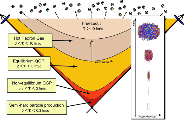
Figure 1: Schematic picture of an ultrarelativistic heavy ion collision with estimated time scales. Figure taken from Ref. [25].

The initial stages

The initial state of a heavy ion collision remains the most uncertain element of the theoretical picture described in Sec. 2.1, as it is the domain of non-perturbative quantum field theory. Nevertheless, crucial insights into the relevant physics were formulated already in the early 1980s. Two heavy ions approaching one another at ultrarelativistic velocity are highly Lorentz contracted along the direction of motion, with the factor $\gamma=1/\sqrt{1-v^{2}/c^{2}}\sim 100$ typical for RHIC conditions and more than $1000$ for the LHC. The ultrarelativistic nature of the collisions has critically important consequences for the physics of the subsequent evolution.

The fundamental observations originate in Refs. [26, 27, 28] and rely on the notion of nuclear transparency, which states that the highly Lorentz-contracted nuclei essentially pass through each other, creating a central fragmentation region of energy density high enough for a deconfined state of QCD matter to form. The contracted nuclei are treated as if they were of infinite transverse extent, with no dynamics in the transverse plane. The baryon number of the colliding nuclei is carried away from this region by the receding projectiles, leaving behind a drop of approximately baryon-neutral plasma.

The physical picture developed in Ref. [16] envisages matter moving essentially along the collision axis, which we take to be the z-axis, with velocity $v=z/t$ in the centre of mass frame, in a manner reminiscent of the Hubble expansion of the Universe. This assumption is equivalent to invariance under boosts along the collision axis and it can be tested experimentally. It implies that the number of charged particles per unit rapidity $dN_{\rm ch}/d\eta$ is independent of rapidity in the region $\eta\approx 0$. Experimental data from PHOBOS [29, 30] shown in Fig. 2 demonstrate the emergence of a central plateau region with increasing collision energy in the range $\sqrt{s}=19.6-200$ GeV in the Au-Au system. In consequence, at earliest times, longitudinal expansion dominates the dynamics and the transverse flow builds up only somewhat later. This effect is strongest for central collisions.

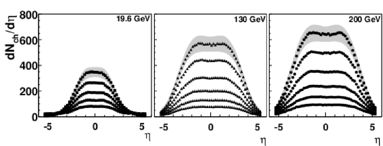
Figure 2: Emergence of a central plateau region in the charge particle production rate in Au-Au collisions for increasing collision energy $\sqrt{s}=19.6,\leavevmode\nobreak\ 130\leavevmode\nobreak\ {\rm and}\leavevmode\nobreak\ 200\leavevmode\nobreak\ \rm GeV$. The grey band represents most central collisions in the $0-6\%$ centrality bin. The plots are taken from Refs. [29, 30].

This idealised picture can be expressed as a set of symmetry assumptions which define Bjorken flow. To do this, it is very convenient to use the proper time $\tau$ and spacetime rapidity $\eta_{s}={\rm arctanh}(z/t)$ coordinates. In terms of these, the Minkowski metric takes the form:

$$ds^{2}=-dt^{2}+dz^{2}+dx_{\perp}^{2}=-d\tau^{2}+\tau^{2}d\eta_{s}^{2}+dx_{\perp}^{2}\leavevmode\nobreak\ ,$$ (1)

where $x_{\perp}=(x,y)$ are coordinates in the transverse plane. The physical idealisations sketched in the previous paragraphs translate to the statement that the physics is independent of spacetime rapidity $\eta_{s}$ as well as the coordinates in the transverse plane. The components of the relativistic flow velocity assume the form $(u^{\mu})=(1,0,0,0)$, with $u_{\mu}u^{\mu}=-1$.

The fundamental local observable which will be the focus of our considerations is the energy-momentum tensor. Under the symmetry assumptions stated above it can be expressed in terms of three functions of the proper time $\tau$:

$$T^{\mu}_{\nu}={\rm diag}\left\{-\mathcal{E}(\tau),\mathcal{P}_{L}(\tau),\mathcal{P}_{T}(\tau),\mathcal{P}_{T}(\tau)\right\}\leavevmode\nobreak\ ,$$ (2)

where $\mathcal{E}$ is the energy density in the local rest-frame, and the eigenvalues $\mathcal{P}_{L},\mathcal{P}_{T}$ are referred to as the longitudinal and transverse pressures. The form of Eq. (2) does not rely on the applicability of a hydrodynamic description, as it is determined only by the symmetry assumptions reviewed above.

One can parametrise the eigenvalues $\mathcal{P}_{L},\mathcal{P}_{T}$ as

$$\mathcal{P}_{L}=\mathcal{P}\left(1-\frac{2}{3}\mathcal{A}\right),\qquad\mathcal{P}_{T}=\mathcal{P}\left(1+\frac{1}{3}\mathcal{A}\right)\leavevmode\nobreak\ ,$$ (3)

where

$$\mathcal{P}\equiv\frac{1}{3}\left(\mathcal{P}_{L}+2\mathcal{P}_{T}\right)$$ (4)

is naturally interpreted as the average pressure, while $\mathcal{A}$ reflects the pressure anisotropy

$$\mathcal{A}\equiv\frac{\mathcal{P}_{L}-\mathcal{P}_{T}}{\mathcal{P}}.$$ (5)

The pressure anisotropy is a measure of distance from equilibrium, or more precisely, from spatial isotropy, which is a necessary condition for equilibrium in the absence of external fields.

Conformal symmetry

Since QCD at high energies is approximately scale invariant, it is natural to impose conformal symmetry to simplify the mathematical description. This is a very powerful assumption which requires tracelessness of the energy momentum tensor $T^{\mu}_{\mu}=0$, and implies that $\mathcal{P}=\mathcal{E}/3$. The energy-momentum tensor for conformal Bjorken flow can thus be expressed in terms of two functions of proper time, $\mathcal{E}$ and $\mathcal{A}$. Conservation of the energy momentum tensor

$$\nabla_{\mu}T^{\mu\nu}=0$$ (6)

relates the pressure anisotropy to the logarithmic derivative of the energy density:

$$\mathcal{A}(\tau)=6\left(1+\frac{3}{4}\tau\partial_{\tau}\ln\mathcal{E}\right)\leavevmode\nobreak\ .$$ (7)

For conformal systems it is also very convenient to introduce the concept of effective temperature $T(\tau)$, defined by

$$\mathcal{E}=C_{e}T^{4}\leavevmode\nobreak\ ,$$ (8)

where $C_{e}$ is a constant which depends on the number of degrees of freedom. This equation has the form of a conformal equation of state, so that in an equilibrium state $T$ is the thermodynamic temperature. Away from equilibrium Eq. (8) defines $T$ as equal to the temperature of an equilibrium state with the same energy density.

At asymptotically late times the system approaches local thermodynamic equilibrium, so the pressure anisotropy tends to zero and the energy-momentum tensor in Eq. (2) approaches the perfect-fluid form. The way this happens is determined by the microscopic dynamics which governs the evolution of the pressure anisotropy. Once $\mathcal{A}(\tau)$ is known, the energy density is determined by Eq. (7) up to a single integration constant which sets the scale. In this sense, for Bjorken flow the dynamics is captured by the pressure anisotropy. In the late time limit, if we set $\mathcal{A}\approx 0$, then Eq. (6) determines the effective temperature

$$T=\frac{\Lambda}{(\Lambda\tau)^{1/3}}$$ (9)

where $\Lambda$ is the integration constant containing information about the initial condition. This is a consequence of local equilibrium and the conservation of energy-momentum, so it is valid regardless of any dynamical details.

Prehydrodynamic evolution and the hydrodynamic attractor

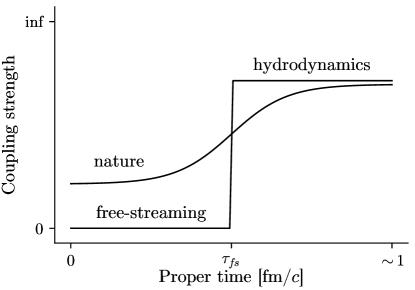
Figure 3: Schematic picture of a coupling evolution and the transition to hydrodynamics. Figure taken from Ref. [31].

The early stages of QGP dynamics are not well understood at this time. At a qualitative level one may say that the longitudinally expanding, approximately boost-invariant initial state begins to build up transverse pressure and evolves toward local thermal equilibrium. The main challenge is to understand how this state becomes amenable to a description in terms of hydrodynamics. Consistency with observation suggests that this happens on a timescale of about $0.3\leq\tau\leq 1\leavevmode\nobreak\ \rm fm/c$, when the system is still very anisotropic, and hydrodynamics in the usual sense would not be expected to apply. And yet, one has to accept as fact that hydrodynamic simulations capture many essential features of QGP dynamics.

An important point is that gluon self-interactions are not only responsible for asymptotic freedom, but also for their proliferation, which leads to a dense medium. Attempts to describe it in terms of quasiparticles require parameter values such that the mean free path of constituents cannot be large compared to their de Broglie wavelength [3]. This implies that despite the weakness of parton interactions at small distances, strong collective effects should be expected and are seen as playing a key role in the thermalisation process [32, 33]. The precise way this plays out is still the subject of current research, but it is feasible that following a regime where a field-theoretical description is necessary, the system enters a stage which can be described by approximately free-streaming quasiparticles (for recent reviews please see e.g. Refs. [34, 23, 4]). The simplest way to model this situation is to adopt a "step-function approach" and assume that particles free stream for some time $\tau_{\rm fs}$, and at that point the description switches to hydrodynamic evolution at a time when the expanding plasma system is still far from equilibrium. This is schematically depicted in Fig. 3.

The successful application of hydrodynamic models in such far-from-equilibrium situations implies that the complexity of initial states is rapidly reduced within a very short interval of proper-time. Since this happens for all initial states, the system can be said to reach a far-from-equilibrium hydrodynamic attractor. In the context of boost-invariant flow this implies that any potentially complex dynamics of the pressure anisotropy should give way to universal features already at very early times, very far from the perfect fluid domain. Thus, hydrodynamic attractors enter the picture as an interface to the hydrodynamic stage. In principle, this attractor could describe free streaming at the very earliest times, but it is not known whether this is the case or not. At present we have to resort to various models and uncontrolled approximations, some of which (such as kinetic theory) imply free streaming, while others do not.

In the next seven Sections we will review the early-time dynamics and the appearance of far-from-equilibrium attractors in various model systems. We will also address the important issue of relaxing some of the symmetry assumptions which we have described in this Section.

Hydrodynamic models of equilibration

The appearance of attractors at the early stages of QGP dynamics can be understood most easily in the context of what we refer to here as hydrodynamic models of equilibration. This Section reviews the necessary conceptual framework by clarifying the relationship between hydrodynamic behaviour and this simplest class of models where its emergence can be studied. Since this review is focused on attractors, the aim of this section is not to introduce the subject of relativistic hydrodynamics, which is well covered by the existing sources (see e.g.  [35, 22, 36]), but rather to present a perspective which is useful for understanding hydrodynamic attractors.

Conservation laws

Hydrodynamic behaviour follows from conservation laws, the most fundamental ones being those which express spacetime symmetries. In the relativistic setting they take the form of the conservation law of the energy-momentum tensor:

$$\nabla_{\mu}T^{\mu\nu}=0\leavevmode\nobreak\ .$$ (10)

In the context of a microscopic theory, such as a quantum field theory, $T^{\mu\nu}$ above would refer to the expectation value of the energy-momentum operator in some state, while in a kinetic theory model this would be a suitable moment of the distribution function (see Section 5). When the system is in local equilibrium, this quantity can be expressed in the perfect fluid form, which is just a constant boost of its value at equilibrium:

$$T_{\mu\nu}=\mathcal{E}u_{\mu}u_{\nu}+\mathcal{P}\Delta_{\mu\nu}\,,$$ (11)

where $\Delta_{\mu\nu}=g_{\mu\nu}+u_{\mu}u_{\nu}$ and $u$ is the boost parameter – the relativistic velocity. Throughout this review, the metric $g$ is assumed to be that of flat Minkowski space. The quantities $\mathcal{E}$ and $\mathcal{P}$ are scalars which can be interpreted as the energy density and pressure in the local rest frame. They are usually expressed in terms of the local effective temperature $T$ through equations of state. The effective temperature and flow velocity are then referred to as the hydrodynamic variables. Due to the normalisation condition of the four-velocity ($u\cdot u=-1$), there are four independent variables.

If the system is not in global equilibrium, the four hydrodynamic variables are no longer constant and energy momentum tensor will depart from the perfect fluid form

$$T_{\mu\nu}=\mathcal{E}u_{\mu}u_{\nu}+\mathcal{P}\Delta_{\mu\nu}+\pi^{\mu\nu}.$$ (12)

The correction $\pi^{\mu\nu}$ appearing above will be referred to as the dissipative tensor. This tensor vanishes unless the hydrodynamic variables vary in spacetime, so one expects that sufficiently close to equilibrium it can be expressed as a series of terms involving derivatives of the hydrodynamic variables; this series is referred to as the hydrodynamic gradient expansion. The gradient expansion provides an asymptotic description of a given flow sufficiently close to equilibrium. This asymptotic behaviour is strongly constrained by symmetries and is thus common to many microscopic systems.

The definition of the hydrodynamic variables is physically unambiguous only in global equilibrium. In general, one can redefine them according to

$$\mathcal{E}=\tilde{\mathcal{E}}+\delta\mathcal{E},\quad u^{\mu}=\tilde{u}^{\mu}+\delta u^{\mu}\leavevmode\nobreak\ .$$ (13)

In the context of the gradient expansion the delta-terms appearing above can be thought of as being of order one or higher. Up to some finite order such redefinitions can be used to impose so-called hydrodynamic frame conditions which eliminate some components of the energy-momentum tensor. A very convenient requirement of this type is the Landau condition

$$u_{\mu}\pi^{\mu\nu}=0\,.$$ (14)

Unless stated otherwise, in this review we will be assuming that this choice has been made.

Modelling hydrodynamics

The basic idea of hydrodynamic models is to adopt the hydrodynamic variables $(u^{\mu})$ and $T$ as independent classical fields in an effective description of the dynamics of the energy-momentum tensor. Hydrodynamic models then view the conservation equations Eq. (10) not as a statement about the expectation value of energy-momentum in a microscopic theory, but rather as a set of four evolution equations which determine the dynamics of the four hydrodynamic variables. With the energy-momentum tensor in the form given in Eq. (11), this leads to the relativistic theory of perfect fluids.

In order to incorporate dissipation one needs to express the dissipative tensor $\pi^{\mu\nu}$ in Eq. (12) in terms of the hydrodynamic variables and their gradients. It is natural to do this by using the gradient expansion, which from this perspective is the most general parametrisation of near-equilibrium behaviour, including all the terms allowed by symmetries.

In conformal theories it is very convenient to express gradients in terms of Weyl-covariant derivative $\mathcal{D}_{\mu}$ which differs from the ordinary derivative by terms involving the four-velocity $u$ and its gradient. Its general definition and properties can be found in Ref. [37] (see also the appendix E of Ref. [22] for a brief summary). The simplest possibility is to set

$$\pi_{\mu\nu}=-\eta\sigma_{\mu\nu}\equiv-\eta\left({\mathcal{D}}_{\mu}u_{\nu}+{\mathcal{D}}_{\nu}u_{\mu}\right)=-\eta\left(\partial_{\mu}u_{\nu}+\partial_{\nu}u_{\mu}-\frac{2}{3}\Delta_{\mu\nu}\partial_{\alpha}u^{\alpha}\right)\leavevmode\nobreak\ ,$$ (15)

which is the unique term of first order in gradients which is consistent with Lorentz and conformal invariance. The coefficient $\eta$ appearing here is the shear viscosity, which is a scalar function of the effective temperature. The resulting model is the relativistic generalisation of Navier-Stokes theory. In contrast to non-relativistic case, this theory is acausal, because it possesses solutions which propagate at arbitrarily large velocities. In consequence, this theory is also unstable [38, 39, 35, 40].

To obtain a consistent and practically useful dynamical model one needs to provide a prescription for augmenting the conservation equations Eq. (10) in such a way as to be able to calculate the time evolution of arbitrary initial data. This prescription has to guarantee stability under perturbations of equilibrium, as well as causality of propagation. It must also ensure the correct asymptotic behaviour as equilibrium is approached, which is given by Eq. (15). These requirements are very strong, and precious few examples exist where they have been proved to be satisfied (see Refs. [41, 42, 43, 44, 45]). In the remainder of this Section we review the most widely-used approaches, where they can be satisfied at least at the linearised level.

The MIS approach

The MIS approach [9, 10] does not assume an explicit form of the dissipative tensor in terms of gradients of the hydrodynamic variables. Instead, it posits a separate set of partial differential equations for the dissipative tensor. These are formulated in such a way as to possess asymptotic solutions in the form of the gradient expansion parametrised in terms of some finite number of scalar parameters.

In the simplest variant of MIS theory the dissipative tensor satisfies equations of the form of a relaxation equation

$$(\tau_{\Pi}{\mathcal{D}}+1)\pi_{\mu\nu}=-\eta\sigma^{\mu\nu}+\dots$$ (16)

where ${\mathcal{D}}\equiv u^{\mu}{\mathcal{D}}_{\mu}$. The properties of the Weyl-covariant derivative ensure that the Landau condition is preserved under time evolution. One may also include additional terms in this equation, as discussed below. As written, this model guarantees stability as well as causality at the linearised level, as long as the relaxation time is large enough, satisfying the bound (see e.g. Ref.[35, 22])

$$T\tau_{\pi}>2\eta/s\leavevmode\nobreak\ .$$ (17)

Causality and stability at the nonlinear level are much more challenging to establish, as discussed e.g. in Ref. [45].

The solution to the relaxation equation  (16) can be formally expanded in gradients:

$${\pi^{\mu\nu}} = -\eta{\sigma^{\mu\nu}}+\tau_{\Pi}{\mathcal{D}}\left(\eta{\sigma^{\mu\nu}}\right)+\ldots$$ (18)

where the ellipsis denotes terms of third and higher orders. The leading term is of the Navier-Stokes form given in Eq. (15). The second and higher order terms are affected by the precise set of terms chosen for the right hand side of Eq. (16). In order to view a hydrodynamic model of equilibration as an effective description of some underlying theory, one needs to have a means of matching the two. This can be done using the gradient expansion which, as a perturbative series around the state of global equilibrium, can be computed in any dynamical theory – at least in principle. This circumstance makes it possible to match parameters by comparing terms of the gradient expansion calculated in a microscopic theory with analogous terms calculated in a hydrodynamic model [46]. For this to be generally possible at a given order in the gradient expansion, the series in Eq. (18) would have to include all terms allowed by Lorentz (and conformal) symmetry at this order. Eq. (16) can match any microscopic model to first order in gradients, but if one wishes to have the option to match to second order, additional terms are needed. In Ref. [47] the complete set of second order terms which are consistent with Lorentz and conformal covariance was determined. They can be matched by the gradient expansion of the following relaxation equation

$$\left(\tau_{\pi}{\mathcal{D}}+1\right)\pi^{\mu\nu}=-\eta\sigma^{\mu\nu}+\lambda_{1}{\pi^{\langle\mu}}_{\lambda}\pi^{\nu\rangle\lambda}+\lambda_{2}{\pi^{\langle\mu}}_{\lambda}\omega^{\nu\rangle\lambda}+\lambda_{3}{\omega^{\langle\mu}}_{\lambda}\omega^{\nu\rangle\lambda}\,.$$ (19)

Here $\lambda_{1},\lambda_{2},\lambda_{3}$ are additional transport coefficients which guarantee matching to second order in gradients ,

$$\omega^{\mu\nu}=\frac{1}{2}\left({\mathcal{D}}^{\mu}u^{\nu}-{\mathcal{D}}^{\nu}u^{\mu}\right),$$ (20)

is the kinetic vorticity, and the angular brackets are defined as

$${}^{\langle}A^{\mu\nu\rangle}\equiv A^{\langle\mu\nu\rangle}=\frac{1}{2}\Delta^{\mu\alpha}\Delta^{\nu\beta}\left(A_{\alpha\beta}+A_{\beta\alpha}\right)-\frac{1}{3}\Delta^{\mu\nu}\Delta^{\alpha\beta}A_{\alpha\beta}.$$ (21)

In the remainder of this review when talking about MIS theory we will have in mind the above form of the relaxation equations, sometimes referred to as the BRSSS equations. It is worth pointing out that while Eq. (19) is general enough so that its gradient expansion includes all the terms in Eq. (18) with arbitrary coefficients, it is not unique [47].

Finally, we note that while MIS theory is the most widely-used framework for building models of hydrodynamics, other approaches exist, such as anisotropic hydrodynamics (for a review and references see e.g. Ref. [22]).

Lessons from linear response

Important insights into nonequilibrium dynamics follow from linearisation around the state of global equilibrium. For our purposes it is enough to consider here the state of homogeneous equilibrium (non-rotating, without any external fields). The hydrodynamic variables which solve the linearised equations are then proportional to the harmonic factor $\exp\left(-i\omega(k)t+i\vec{k}\cdot\vec{x}\right)$. The dispersion relations which define the different solutions (modes) fall into two categories: the hydrodynamic modes whose frequency vanishes with at long wavelengths, $\lim_{k\rightarrow 0}\omega(k)=0$, and the nonhydrodynamic modes which are gapped: $\lim_{k\rightarrow 0}\omega(k)\neq 0$. This gap – the frequency at vanishing wave vector $k$ – sets the asymptotic damping rate of the transient modes. The damping of the hydrodynamic modes diminishes with $k$, so modes of long wavelengths are weakly damped.

For example, linearisation of the evolution equations of MIS theory reveals a set of hydrodynamic sound and shear modes

$$\omega_{\rm shear} = -i\frac{\eta}{sT}k^{2}+O(k^{4})\leavevmode\nobreak\ ,$$ (22)

$$\omega_{\rm sound} = \pm\frac{1}{\sqrt{3}}k-\frac{2i}{3}\frac{\eta}{sT}k^{2}+O(k^{3})\leavevmode\nobreak\ ,$$ (23)

as well a some nonhydrodynamic modes which are damped regardless of wavelength: their dispersion relation is $\omega=-i/\tau_{\Pi}+O(k^{2})$. In the limit when the relaxation time vanishes, the nonhydrodynamic modes decouple and this theory reduces to Navier-Stokes theory. A calculation of the velocity of sound (see e.g. Refs. [35, 22]) gives

$$v=\frac{1}{\sqrt{3}}\sqrt{1+4\frac{\eta/s}{T\tau_{\Pi}}}.$$ (24)

The condition Eq. (17) provides a limit on how small the relaxation time can be without violating causality. Thus, a natural way to think of nonhydrodynamic modes is to view them as a regulator [52] (somewhat in the spirit of a “UV-completion” of quantum field theories), with the relaxation time playing the role of a regulator parameter.

This happens not just in MIS-type theories, but in many other hydrodynamic models which are causal at least at the linear level, such as BDNK [41, 44, 53, 20] and HJSW [54]. Indeed, recent results [55, 56] strongly suggest that the presence of nonhydrodynamic modes is a necessary condition for causality. The existence of hydrodynamic modes follows from conservation laws, while the nonhydrodynamic modes are required to maintain causality. The nonhydrodynamic modes account for transient behaviour, while the long-lived hydrodynamic modes express a measure of universality in the approach to equilibrium.

Modeling the non-hydrodynamic sector

The appearance of nonhydrodynamic modes in models of relativistic hydrodynamics mirrors the structure of microscopic theories. However, the analysis of linearised perturbations of microscopic models reveals a much more complicated picture than the simple nonhydrodynamic sector of MIS theory. This happens in models of kinetic theory [57], as well as strongly coupled field theories described using methods based on the AdS/CFT correspondence [58]. In both these cases there is an infinite number of nonhydrodynamic modes, and in the latter case they are not purely decaying. Sufficiently close to equilibrium the details of this sector are not relevant, as the near-equilibrium physics is captured by the hydrodynamic modes [59]. However, in practice models of hydrodynamics are often used further away from equilibrium, so models with different nonhydrodynamic sectors will a priori lead to different results. In such situations one is really probing the physics of the regulator.

This raises the question whether it is possible to engineer hydrodynamic models which mimic nontrivial nonhydrodynamic sectors. An example of such a model was put forward in Ref. [54] and will be referred to as the HJSW model (see also [22, 60, 61]). The motivation behind its formulation was to mimic the behaviour of strongly coupled $\mathcal{N}=4$ SYM theory, where the least-damped transient modes depend very weakly on momentum (a phenomenon known as ultralocality). This leads to an evolution equation for the dissipative tensor of the form

$$\left(\frac{1}{T}\mathcal{D}\right)^{2}\pi_{\mu\nu}+2\Omega_{I}\frac{1}{T}\mathcal{D}\pi_{\mu\nu}+|\Omega|^{2}\pi_{\mu\nu}=-\eta|\Omega|^{2}\sigma_{\mu\nu}-C_{\sigma}\frac{1}{T}\mathcal{D}\left(\eta\sigma_{\mu\nu}\right)+\dots\leavevmode\nobreak\ .$$ (25)

This equation is a replacement for the MIS/BRSSS relaxation equation, Eq. (16). The parameters $\eta,\Omega_{R},\Omega_{I},C_{\sigma}$ play the same role as the transport coefficients appearing in Eq. (16), and $|\Omega|^{2}=\Omega_{R}^{2}+\Omega_{I}^{2}$. The term with parameter $C_{\sigma}$ was introduced to broaden the domain where the theory is stable and causal at the linearised level. The physical meaning of these parameters is partially revealed by formally expanding Eq. (25) in gradients, which yields Eq. (18) with the identification

$$\tau_{\Pi}=\frac{2\Omega_{I}-C_{\sigma}}{|\Omega|^{2}}\frac{1}{T}$$ (26)

and $\eta$ retaining its meaning as the shear viscosity.

Further insight is gained by calculating the dispersion relations for linear perturbations of equilibrium. Apart from the standard hydrodynamic modes we see nonhydrodynamic modes

$$\omega_{\pm}(k)=-i\Omega_{I}\pm\Omega_{R}+O(k)$$ (27)

whose relaxation rate is set by $\Omega_{I}$. In contrast to MIS theory, these modes are not purely decaying: they also oscillate with frequency set by $\Omega_{R}$. This captures the patterns of least-damped quasinormal mode of the black brane appearing in the dual description of ${\mathcal{N}}=4$ SYM theory (see Section 6), where $\Omega_{R}\approx 9.8$ and $\Omega_{I}\approx 8.6$. Of course, in the spirit of hydrodynamics, Eq. (25) could in principle apply to any theory with a similar pattern of nonhydrodynamic modes. Thus, at least at the level of the gradient expansion, this model contains Navier-Stokes theory in the near-equilibrium limit – just like MIS – but provides a different regulator sector. The assumption of ultralocality which has lead to Eq. (25) is a useful simplification, but it is not strictly obeyed in SYM, and can be avoided at the level of hydrodynamic models [62].

The idea of including nonhydrodynamic modes in a deliberate manner has also been the founding concept of the Hydro+ programme [63], which is being actively developed in connection with the search for signals of a critical point in the QCD phase diagram through heavy-ion collisions. Recent work developing this circle of ideas includes Refs. [64, 65].

General frames

Another interesting class of hydrodynamic models was discovered quite recently by Disconzi, Bemfica, Noronha and Kovtun in Refs. [41, 44, 53]. These models, usually referred to by the acronym BDNK, deviate from the MIS approach in that they do not introduce additional hydrodynamic fields beyond those already present in Navier-Stokes theory and rely only on the conservation equations to provide the dynamics.

The basic insight of BDNK was to recognise that the Landau condition, Eq. (14), is not a fundamental requirement, but rather one of many ways of pinning down the definition of the hydrodynamic variables off-equilibrium. So instead of Eq. (15), at first order in gradients one could adopt the following form of the dissipative tensor:

$$\pi_{\mu\nu}=\tau^{\mu\nu}+\mathcal{C}\left(u_{\mu}u_{\nu}+\frac{1}{3}\Delta_{\mu\nu}\right)+\mathcal{Q}_{\mu}u_{\nu}+\mathcal{Q}_{\nu}u_{\mu}$$ (28)

where

$$\tau^{\mu\nu}=-\eta\sigma^{\mu\nu},\quad\mathcal{Q}^{\mu}=-\tau_{\psi}\Delta^{\mu\lambda}{\mathcal{D}}_{\lambda}\mathcal{E},\quad\mathcal{C}=-\tau_{\phi}\mathcal{D}\mathcal{E}$$ (29)

where $\tau_{\phi},\tau_{\psi}$ are new transport coefficients. These additional terms in Eq. (28) (relative to Eq. (15)) could be removed using the frame freedom Eq. (13), which would amount to imposing the Landau condition. No new dynamical fields are introduced: $\tau^{\mu\nu},\mathcal{Q}^{\mu},\mathcal{C}$ are expressed explicitly in terms of the basic hydrodynamical variables $\mathcal{E},u^{\mu}$. Nevertheless, this theory is causal and stable [45] for suitable choices of parameters, because relaxing the Landau frame condition introduces a nonhydrodynamic sector. The structure of this sector turns out to be the same as in MIS theories, but the evolution equations are different and lead to the same physics only close to equilibrium [59]. Models of this type are the subject of a number of interesting recent studies [66, 67, 68, 69, 70, 71].

The general-frame concept can be taken further in the spirit of the MIS approach [20]. The basic idea is to replace Eq. (29) by a set of relaxation equations

$$\tau_{\pi}\mathcal{D}\pi^{\mu\nu}+\pi^{\mu\nu} = -\eta\sigma^{\mu\nu}$$

$$\tau_{Q}{\mathcal{D}}\mathcal{Q}^{\mu}+\mathcal{Q}^{\mu} = -\tau_{\psi}\Delta^{\mu\lambda}{\mathcal{D}}_{\lambda}\mathcal{E}$$

$$\tau_{C}\mathcal{D}\mathcal{C}+\mathcal{C} = -\tau_{\phi}\mathcal{D}\mathcal{E}$$ (30)

with additional transport coefficients $\tau_{\pi},\tau_{Q},\tau_{C}$. The resulting model has more degrees of freedom and a nonhydrodynamic sector which is larger than in either MIS or BDNK, and is of some practical as well as conceptual significance [72, 73]. We will return to it briefly in Section 4, since it offers some additional insights into attractor behaviour.

Attractors in hydrodynamic models

Hydrodynamic attractors were first identified in hydrodynamic models, and subsequently studied in other models of equilibration such as kinetic theory and strongly coupled theories amenable to studies based on the AdS/CFT correspondence. This Section reviews attractors arising in hydrodynamic models of Bjorken flow and introduces a number of concepts which will be used in the remainder of this article.

Bjorken flow in MIS theory

We now turn to the description of Bjorken flow in MIS theory, specifically the BRSSS version [47]. As reviewed in Section 2, the dynamics of the energy-momentum tensor in this case is captured by the pressure anisotropy $\mathcal{A}(\tau)$ and the energy density $\mathcal{E}(\tau)$, or equivalently the effective temperature $T(\tau)$. Conservation of the energy-momentum tensor reduces to Eq. (7), which can be written as the evolution equation for the effective temperature:

$$\tau\partial_{\tau}\log T(\tau)=-\frac{1}{3}+\frac{1}{18}\mathcal{A}(\tau)\leavevmode\nobreak\ ,$$ (31)

while the MIS relaxation equation Eq. (19) becomes an evolution equation for the pressure anisotropy. To write it down most explicitly one needs to take full advantage of the constraints of conformal symmetry.

Conformal symmetry implies that the energy scale is set by the local effective temperature. The transport coefficients are then determined by dimensional analysis 

$$\tau_{\pi}=\frac{C_{\tau\Pi}}{T},\qquad\eta=C_{\eta}s\leavevmode\nobreak\ ,\qquad\lambda_{1}=\frac{C_{\lambda_{1}}}{T\eta}\leavevmode\nobreak\ ,$$ (32)

where $s=4\mathcal{E}/3T$ is the entropy density, up to dimensionless constants $C_{\tau\Pi},C_{\eta},C_{\lambda_{1}}$. These constants can be fitted to experiment, or matched to an underlying microscopic theory in cases where an explicit calculation of the gradient expansion is feasible. An example of such a calculation for the cases of ${\mathcal{N}}=4$ SYM was carried out in Ref. [46, 47] using the AdS/CFT correspondence, with the result

$$C_{\tau\Pi}=\frac{2-\log 2}{2\pi}\leavevmode\nobreak\ ,\qquad C_{\eta}=\frac{1}{4\pi}\leavevmode\nobreak\ ,\qquad C_{\lambda_{1}}=\frac{1}{2\pi}\leavevmode\nobreak\ .$$ (33)

These values provide a useful point of reference as well as an order of magnitude estimate which is sometimes used in hydrodynamic simulations.

Once the transport coefficients are written in the form Eq. (32), the MIS/BRSSS relaxation equation can be written in the form

$$C_{\tau\Pi}\left(\tau\mathcal{A}^{\prime}(\tau)+\frac{2}{9}\mathcal{A}^{2}(\tau)\right)=8C_{\eta}-\tau T(\tau)\left(\mathcal{A}(\tau)+\frac{C_{\lambda}}{12C_{\eta}}\mathcal{A}(\tau)^{2}\right).$$ (34)

The system of two coupled ordinary differential equations, Eq. (31) and Eq. (34) determines the dynamics of Bjorken flow in MIS theory.

Late time asymptotics of Bjorken flow

The evolution equations, Eq. (31) and Eq. (34), can be combined to give a single ODE which determines the dynamics of the effective temperature

$$C_{\tau\Pi}\tau T^{\prime\prime} + \frac{3}{2}\tau\left(\frac{C_{\lambda_{1}}\tau}{C_{\eta}}+\frac{2C_{\tau\Pi}}{T}\right){T^{\prime}}^{2}+\left(\frac{11C_{\tau\Pi}}{3}+\frac{(C_{\eta}+C_{\lambda_{1}})\tau T}{C_{\eta}}\right)T^{\prime}+$$ (35)

$$+ \frac{(2C_{\eta}+C_{\lambda_{1}})T^{2}}{6C_{\eta}}-\frac{4(C_{\eta}-C_{\tau\Pi})T}{9\tau}=0\leavevmode\nobreak\ .$$

It is easy to see that at large proper-times this equation has an asymptotic solution of the form

$$T(\tau)=\frac{\Lambda}{(\Lambda\tau)^{\frac{1}{3}}}\left(1-\frac{2C_{\eta}}{3(\Lambda\tau)^{\frac{2}{3}}}+O\left(\frac{1}{(\Lambda\tau)^{4/3}}\right)\right)\leavevmode\nobreak\ ,$$ (36)

where $\Lambda$ is an integration constant. Since the initial value problem for Eq. (35) allows for the choice of two integration constants, namely the initial temperature and its derivative, it is clear that the asymptotic solution Eq. (36) contains only half the information encoded in the initial state. This is a consequence of dissipation. A complete solution would require augmenting this result with additional terms which depend on the remaining initial data, but vanish faster than any power of proper time. We will return to this important point below in Section 4.6.

Quite generally, dissipation implies an effective loss of information: specifically, a partial loss of memory of the initial state of the system. The initial state can be far from equilibrium and may be characterised by many parameters. On the other hand, the final state of equilibrium is characterised by very few parameters. The asymptotic late-time behaviour of the system will thus be partially independent of the initial state. This process of “information loss” can be studied using modern asymptotic methods. Furthermore, it lies at the heart of the idea of hydrodynamic attractors, which – as we will discuss in detail – is fundamentally the observation that generic initial states evolve into a region of phase space which can be effectively covered by a subset of all possible initial conditions.

Universal variables

In the case of conformal Bjorken flow it is possible to make the notion of information loss described above even sharper by using suitable variables which are correlated in a universal way: variables in which the asymptotic behaviour near equilibrium is completely independent of initial conditions. This is not a typical situation and is only possible due to the very strong symmetry assumptions.

Conformal symmetry suggests using the dimensionless pressure anisotropy $\mathcal{A}$ and introducing the dimensionless variable $w\equiv\tau T$. At late times, when the temperature follows Eq. (9), $w\sim\tau^{2/3}$, so that it can be thought of as a “clock variable”: the proper time in units of local effective temperature. Since the relaxation time $\tau_{\Pi}\sim 1/T$, one also has $w\sim\tau/\tau_{\Pi}$, so one can think of this variable as the proper time in units of the relaxation time. Using these dimensionless variables, the conservation equation (31) can be written as

$$\frac{d\log T}{d\log w}=\frac{\mathcal{A}-\ 6}{\mathcal{A}+12}\leavevmode\nobreak\ ,$$ (37)

and the MIS equation Eq. (34) takes the form

$$C_{\tau\Pi}\left(1+\frac{\mathcal{A}(w)}{12}\right)\mathcal{A^{\prime}}(w)+\left(\frac{C_{\tau\Pi}}{3w}+\frac{C_{\lambda_{1}}}{8C_{\eta}}\right)\mathcal{A}(w)^{2}=\frac{3}{2}\left(\frac{8C_{\eta}}{w}-\mathcal{A}(w)\right)\leavevmode\nobreak\ .$$ (38)

The remarkable point here is that Eq. (38) is a self-contained equation which can be solved independently of the conservation law Eq. (37). Once solutions $\mathcal{A}(w)$ are found, they can be used in Eq. (37) to determine the corresponding evolution of the effective temperature.

For a perfect fluid $\mathcal{A}=0$ and either Eq. (31) or Eq. (37) suffices to determine the solution, leading to Bjorken’s Eq. (9). However, for dissipative systems one must also specify a nontrivial solution of Eq. (38), which depends on the microscopic dynamics of the plasma through the transport coefficients, as well as on the initial state of the system. If a solution $\mathcal{A}(w)$ of Eq. (38) is given, one can integrate Eq. (37) to solve for the effective temperature as a function of $w$:

$$T(w)=\Phi_{\mathcal{A}}(w,w_{0})T(w_{0})\leavevmode\nobreak\ ,$$ (39)

for some initial condition $T(w_{0})$, with the function $\Phi_{\mathcal{A}}$ being

$$\Phi_{\mathcal{A}}(w,w_{0})=\exp\left(\int_{w_{0}}^{w}\frac{dx}{x}\frac{\mathcal{A}(x)-\ 6}{\mathcal{A}(x)+12}\right)\leavevmode\nobreak\ .$$ (40)

The subscript $\mathcal{A}$ which appears above indicates the functional dependence of this quantity on the pressure anisotropy.

The hydrodynamic attractor

It is straightforward to solve Eq. (38) numerically. As expected, at late times all solutions tend to zero as equilibrium is approached. However, a rather striking picture emerges when studying the behaviour of solutions obtained by setting initial conditions at a sequence of diminishing initial values of $w$, as seen in Fig. 4. It is evident that the solution curves rapidly approach a distinguished locus, which is referred to as a far-from-equilibrium attractor [14]. This attractor curve is determined uniquely by this procedure, and will be denoted by $\mathcal{A}_{\star}$. It is the extension of the hydrodynamic attractor expected near equilibrium into the early-time, nonequilibrium region.

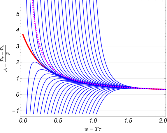
Figure 4: Some solutions of Eq. (38) (blue lines) plotted together with the attractor (red line); the dashed magenta line represents second order viscous hydrodynamics.

It is physically important that solutions initialised off the attractor approach it rapidly while the pressure anisotropy is high and the system is still far from equilibrium. This fact leads to a potential explanation of the early thermalisation puzzle, as we will argue in the following. Note also that solutions which start out below the attractor are initially driven away from equilibrium toward the attractor. As discussed further below, this is a consequence of the strong longitudinal expansion.

The emerging picture is that for a given range of initial conditions, apart from an initial transient, the function $\mathcal{A}(w)$ quickly approaches a universal attractor $\mathcal{A}_{\star}(w)$ which is determined by the microscopic theory under consideration. We assume that the physically interesting range of initial conditions is in the basin of attraction of this unique attractor. This suggests that it should be a good approximation to replace the form of the pressure anisotropy $\mathcal{A}(w)$, as it appears in Eq. (37), by the attractor $\mathcal{A}_{\star}(w)$:

$$T(w)\approx\Phi_{\mathcal{A}_{\star}}(w,w_{0})T(w_{0})\leavevmode\nobreak\ .$$ (41)

Within such an approximation, the temperature at late times is determined by the temperature at early times alone: the remaining dependence on the initial state is neglected by assuming that the effective dynamics of the system is captured by its attractor, apart from a negligible initial transient.

The attractor apparent in the pressure anisotropy $\mathcal{A}(w)$ is particularly striking, but it is a manifestation of an intrinsic feature of this dynamical system, as well as many other like it, however one chooses to describe them. It also has implications for other observables, such as the speed of sound away from equilibrium [75].

The qualitative picture seen in Fig. 4 is typical of Bjorken flow in many models of equilibration, including various extensions of MIS theory, anisotropic hydrodynamics [76, 77], kinetic theory as well as strongly coupled ${\mathcal{N}}=4$ SYM theory. Before reviewing some of them, we will try to understand the features seen in this plot in a quantitative way, using asymptotic methods to extract the relevant physics from Eq. (38).

Early time behaviour

As it is clear from Fig. 4, at small values of $w$ generic solutions are divergent, apart from the attractor which is regular there. It is straightforward to check that if we assume that the pressure anisotropy approaches a finite, constant value $\mathcal{A}_{\pm}$ as $w\rightarrow{0}$, then the only possible values consistent with Eq. (38) are

$$\mathcal{A}_{\pm}=\pm 6\sqrt{C_{\eta}/C_{\tau\Pi}}\leavevmode\nobreak\ .$$ (42)

The negative option is unstable, it acts as a repulsor; we will not discuss it further here. The positive value provides the initial condition which can be used to determine the attractor numerically.

The early-time behaviour of regular solutions of Eq. (38) can be studied analytically through a convergent series expansion in powers of $w$ [14, 78, 79]

$${\mathcal{A}_{\star}}(w)=\sum_{n=0}^{\infty}c_{n}w^{n}=6\sqrt{\frac{C_{\eta}}{C_{\tau\Pi}}}-\frac{9(C_{\lambda_{1}}+2\sqrt{C_{\eta}C_{\tau\Pi}})}{C_{\tau\Pi}(2C_{\tau\Pi}+9\sqrt{C_{\eta}C_{\tau\Pi}})}w+\cdots$$ (43)

In the following we will denote the attractor solution by $\mathcal{A}_{\star}$. The remaining solutions of Eq. (38) diverge at $w=0$, but are seen to approach the attractor rapidly. From a physical perspective it is very important to understand how exactly this happens and what is the reason for it. One can look for solutions of the form

$$\mathcal{A}(w)={\mathcal{A}_{\star}}(w)+\delta\mathcal{A}(w)$$ (44)

where $\delta\mathcal{A}(w)$ is dominant for $w$ approaching zero. The equation of motion Eq. (38) then takes the approximate form

$$w\delta\mathcal{A}^{\prime}(w)+4\delta\mathcal{A}(w)=0\leavevmode\nobreak\ ,$$ (45)

which gives $\delta\mathcal{A}\sim w^{-4}$. This result is independent of the transport coefficients, which suggests a kinematic origin of this phenomenon. More specifically, the physical mechanism behind it can be identified with the strong longitudinal expansion of the system. The implications of this fact will be discussed in Section 9.

Late time behaviour

At large values of $w$, all solutions plotted in Fig. 4 approach the curve corresponding to the leading order of the gradient expansion. This can be seen directly in Eq. (38) by noting that as $w\rightarrow\infty$ both terms on the left hand side of are subdominant, so that the leading asymptotic behaviour is

$$\mathcal{A}(w)\sim\frac{8C_{\eta}}{w}\,.$$ (46)

Just as the late-time solution of Eq. (9), this implies a loss of initial state information, because Eq. (38) which governs the dynamics of the pressure anisotropy requires an initial condition, so a general solution would contain a single integration constant. This information is completely absent from the asymptotic solution Eq. (46), which is completely universal, identical for all initial conditions.

As an aside, it is amusing to note that the leading asymptotic behaviour of the pressure anisotropy can be made not just independent of the initial conditions, but even across different theories, which at this order differ only by the value of $\eta/s$. Indeed, defining $\tilde{w}\equiv w/8C_{\eta}$, the asymptotics of the pressure anisotropy in any conformal theory are simply $\mathcal{A}\sim 1/\tilde{w}$ [80]. This observation has found applications in situations where the late-time behaviours of different theories are compared.

The leading asymptotic behaviour of the pressure anisotropy captured by Eq. (46) is corrected by an infinite series of subleading terms:

$$\mathcal{A}(w)=\sum_{k=1}^{\infty}\frac{a_{k}}{w^{k}}$$ (47)

with

$$a_{1}=8C_{\eta},\quad a_{2}=\frac{16}{3}\,C_{\eta}(C_{\tau\Pi}-C_{\lambda_{1}})\leavevmode\nobreak\ .$$ (48)

Each term appearing here corresponds to a specific order of the gradient expansion. If this series is truncated, one obtains an approximation which one would like to identify with the hydrodynamic prediction for the asymptotic behaviour of $\mathcal{A}(w)$. There is an important subtlety however: the series appearing in Eq. (47) has a vanishing radius of convergence. This will be discussed at length below, but for the moment we will adopt a pragmatic attitude and simply truncate the expansion, keeping only a couple of the leading terms.

It is important to realise that there are corrections to Eq. (47) which are not of the form of a power of $1/w$ – instead, they are damped exponentially in the limit of large $w$. To see this, one can linearise this equation around the truncated asymptotic solution

$$\mathcal{A}(w)=\frac{a_{1}}{w}+\frac{a_{2}}{w^{2}}+\delta\mathcal{A}(w)\leavevmode\nobreak\ ,$$ (49)

by treating $\delta\mathcal{A}$ as small. This leads to the equation

$$\delta\mathcal{A}^{\prime}(w)+\left(\frac{3}{2C_{\tau\Pi}}+\frac{2C_{\lambda_{1}}-C_{\eta}}{C_{\tau\Pi}}\frac{1}{w}+O\left(\frac{1}{w^{2}}\right)\right)\delta\mathcal{A}=0\leavevmode\nobreak\ ,$$ (50)

whose solution is

$$\delta\mathcal{A}(w)=\sigma w^{\frac{C_{\eta}-2C_{\lambda_{1}}}{C_{\tau\Pi}}}e^{-\frac{3w}{2C_{\tau\Pi}}}\left(1+O\left(\frac{1}{w}\right)\right)\leavevmode\nobreak\ ,$$ (51)

where $\sigma$ is an integration constant. A more systematic analysis along the lines sketched above reveals solutions of the form of a transseries [14, 60, 81]:

$$\mathcal{A}(w)=\sum_{m=0}^{\infty}\sigma^{m}e^{-mAw}\Phi_{m}(w)\leavevmode\nobreak\ ,$$ (52)

where

$$\Phi_{m}(w)=w^{m\beta}\sum_{n=0}^{\infty}\frac{a^{(m)}_{n}}{w^{n}}\leavevmode\nobreak\ ,$$ (53)

with

$$A=\frac{3}{2C_{\tau\Pi}}\leavevmode\nobreak\ ,\qquad\beta=\frac{C_{\eta}-2C_{\lambda_{1}}}{C_{\tau\Pi}}\leavevmode\nobreak\ .$$ (54)

and $\Phi_{0}(w)$ is just the series Eq. (47). Each transseries sector provides a set of corrections weighted by a power of an exponential damping factor. The damping rate is set by the relaxation time – the constant factor of $3/2$ is explained in Ref. [82]. Crucially, each transseries sector is also weighted by a power of the undetermined transseries parameter – the integration constant $\sigma$. This integration constant can in principle be determined by setting an initial condition, but that information is exponentially dissipated away in the course of evolution. The transient effects of the nontrivial transseries sectors can actually be seen in numerical experiments [83]. It is important to note that the presence of the transseries sectors is a consequence of the presence of nonhydrodynamic modes in MIS theory. This connection is quite general and will manifest itself a number of times in the following.

The transseries structure is a beautiful metaphor of how information about the initial state is dissipated in the course of evolution as the system approaches equilibrium: this data is effectively lost due to the exponential damping, leaving only a universal hydrodynamic tail: the hydrodynamic attractor. The early-time $1/w^{4}$, expansion-driven approach to the attractor is replaced at later times by the exponential nonhydrodynamic mode decay whose rate is set by the relaxation time.

Determining the attractor

While there exist hydrodynamic models where the attractor can be found exactly [84, 85], in general attractors can be found be studying the behaviour of multiple solutions obtained by numerical means. In the simple case of Bjorken flow in conformal MIS theory this can be done by setting initial conditions at decreasing values of $w$, as illustrated in Fig. 4.

Another approach to capturing the attractor is a variant of the slow-roll approximation best known in the context of inflationary cosmology [86, 87]. This method is approximate, but can be pursued analytically. The idea is to treat the derivative term in Eq. (38) as a perturbation, which ensures the regularity of the obtained solution at $w=0$. This can be implemented systematically by inserting a formal gradient-counting parameter $\epsilon$ into Eq. (38) and seeking a solution as a series in this quantity. The zeroth order solution is determined by a quadratic equation. The attractor solution corresponds to positive root, and one finds [14]

$$\mathcal{A}_{\rm slowroll}(w)=\frac{6}{8C_{\tau\Pi}+\frac{3C_{\lambda_{1}}w}{C_{\eta}}}\sqrt{64C_{\eta}C_{\tau\Pi}+24C_{\lambda_{1}}w+9w^{2}}\leavevmode\nobreak\ .$$ (55)

This is just the nullcline of Eq. (38). Corrections are easily calculated and provide a very accurate representation of the attractor, but its analytic form quickly becomes very complex.

Another way to obtain approximate attractors analytically in certain hydrodynamic models was proposed in [88], where the authors considered a family of relaxation equations of the form

$$\frac{d\pi}{d\tau}=-\frac{\pi}{\tau_{\pi}}+\frac{1}{\tau}\left[\frac{4}{3}\beta_{\pi}-\left(\lambda+\frac{4}{3}\right)\pi-\chi\frac{\pi^{2}}{\beta_{\pi}}\right]\leavevmode\nobreak\ ,$$ (56)

where $\pi\equiv\mathcal{E}\mathcal{A}$. By suitable choices of the parameters $\beta_{\pi}$, $\tau_{\pi}$, $\lambda$ and $\chi$ one can describe the original MIS model [10], the DNMR model [89] or the "third-order" model of Ref. [90]. All three models possess an attractor solution, but it can only be found numerically. In a conformal theory, the relaxation time is determined by the effective temperature, i.e. $\tau_{\pi}\sim 1/T(\tau)$. One can obtain an analytic approximation of the attractor by treating this dependence in a sort of “mean field” spirit. Instead of keeping the exact temperature dependence the authors of Ref. [88] study three possible options which amount to taking the temperature to be constant, or taking one or two terms in the expansion given in Eq. (36). In each of these cases one can obtain a general analytic solution to Eq. (56), which depends on an integration constant. It is possible to choose this integration constant to obtain a solution regular at $w=0$. This solution provides a rather good approximation to the numerically calculated attractor, with the error not larger than $3\%$ [88]. This approximate attractor solution was used in practice for the computations of thermal particle production [91].

Further analytic results for boost-invariant attractors can be found in Refs. [92, 84, 93].

We will also describe two systematic approaches to finding attractors in an approximate way. One is based directly on the gradient expansion, and leads to some very interesting developments which we review in the following subsection. The other, perhaps the most general approach to identifying attractors, albeit purely numerically, involves studying sets of solutions on time slices of phase space; it will be described in Section 7.

The gradient expansion at large orders

We now turn to an important point of both mathematical and physical significance: the infinite series appearing in Eq. (52) have a vanishing radius of convergence. At sufficiently late times, the asymptotic behaviour of all solutions is given by the leading order of the gradient expansion, which corresponds to Navier-Stokes theory. In many cases it has been possible to calculate a large number of terms, which offers the possibility to extend the late-time approximation of the attractor toward early times. This was studied in the case of the large proper time expansion of ${\mathcal{N}}=4$ SYM in Ref. [94] where the series was found to have a vanishing radius of convergence. It was subsequently found that such expansions diverge in many other cases, including models of hydrodynamics [14, 60] and kinetic theory [95, 80, 96]. It has been demonstrated that in the context of MIS theory the gradient expansion has a vanishing radius of convergence also beyond the relatively simple setting of Bjorken flow, and it can only be avoided by fine-tuning of the initial conditions [97, 98]. In fact, the only known example of where the hydrodynamic gradient expansion is convergent for generic initial conditions occurs for Bjorken flow in the model of an ultrarelativistic gas of hard spheres of Ref. [84]. The implication of these findings is that the gradient series does not define a unique solution. However, it captures the asymptotic behaviour of all solutions in the late-time limit.

The simplest approach to such divergent asymptotic series is truncation at low order, as we have been tacitly assuming until now. It is known from countless examples (such as the Stirling formula for the Gamma function $\Gamma(z)$ at large values of $|z|$) that keeping only the leading terms of a divergent asymptotic series often gives excellent results also quite far from the asymptotic limit. This can be made quite precise using the notion of optimal truncation [99]. While this approach is very useful in practice, from a conceptual point of view it is very interesting and rewarding to examine the nature of the divergence in more detail, since it reveals the physics behind it.

The gradient expansion of the pressure anisotropy is of the form

$$\mathcal{A}(w)=\sum_{n=0}^{\infty}\frac{a_{n}}{w^{n}}\leavevmode\nobreak\ ,$$ (57)

where the leading terms can be read off from Eq. (46). When referring to this series in the case of MIS, for definiteness we will assume numerical values for the coefficients $a_{n}$ given in Eq. (47). It is straightforward to compute hundreds of these coefficients numerically. Simple convergence tests lead to the conclusion that the series is divergent factorially (see Fig. 5): at large $n$, up to a constant factor, one has

$$a_{n}\sim\Gamma(n+\beta)A^{-n},$$ (58)

where $A,\beta$ are constants which carry important information about the physics. In particular, the quantity $A$ reflects the damping rate ot transient, nonhydrodynamic effects. Since Eq. (58) arises in many contexts, $A$ is referred to by various names. We will follow Dingle and refer to is as the singulant [100]. In the case of MIS theory $A=3/2C_{\tau_{\Pi}}$, which shows that the divergence originates in the nonhydrodynamic sector.

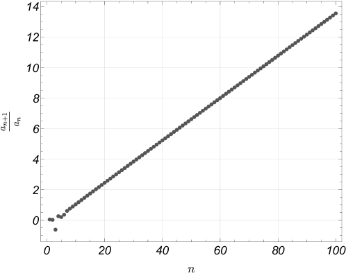
Figure 5: The ratio of the coefficients of the gradient expansion Eq. (57).

There is a large and growing body of work aimed at understating the role of corrections to asymptotic series such as Eq. (57), sometime referred to as “asymptotics beyond all orders” [101]. An effective approach to this problem is to consider “resumming” the series in Eq. (57). By this one means finding a function whose asymptotic expansion matches the original series (see e.g. [102]). Given a factorially divergent sequence $\{c_{n}\}$ this can be done by Borel summation, whose basic idea is captured by the formal manipulation

$$\sum_{n=0}^{\infty}c_{n}=\sum_{n=0}^{\infty}c_{n}\underbrace{\left(\frac{1}{n!}\int_{0}^{\infty}t^{n}e^{-t}dt\right)}_{1}=\int_{0}^{\infty}\underbrace{\left(\sum_{n=0}^{\infty}\frac{c_{n}}{n!}\right)}_{\mathrm{Borel\ transform}}t^{n}e^{-t}dt.$$ (59)

To implement this idea in practice, one first defines the Borel transform of the original factorially divergent series Eq. (57) by

$$\mathcal{BA}(\xi)=\sum_{n=1}^{\infty}\frac{a_{n}}{n!}\xi^{n}\leavevmode\nobreak\ ,$$ (60)

which defines an analytic function inside a disc of radius $|A|$ at the origin. The Borel sum of the original divergent series is defined by the inverse Borel transform

$$\mathcal{A}_{\rm sum}(w)=w\int_{\mathcal{C}}d\xi\,e^{-w\xi}\,\widetilde{\mathcal{BA}}(\xi)\leavevmode\nobreak\ .$$ (61)

The tilde over the Borel transform indicates that the domain where the series Eq. (60) is defined will need to be extended by means of analytic continuation so that one can find a contour $\mathcal{C}$ which extends to infinity.

In most cases of interest one cannot carry out this prescription exactly. Typically, the number of coefficients $a_{n}$ which are available in practice is finite, and the coefficients which are available are often given numerically with some finite precision. One also has to rely on approximate methods of analytic continuation. The quality of this procedure is also critically important for the accuracy of the result of the resummation [103, 104, 105, 106].

The most straightforward and widely-used way to carry out the required analytic continuation is to adopt the Padé approximant

$$\mathcal{BA}_{\rm Pade}(\xi)=\frac{P_{m}(\xi)}{Q_{n}(\xi)}\leavevmode\nobreak\ ,$$ (62)

where $P_{m}(\xi)$ and $Q_{n}(\xi)$ are polynomials of degree $m$, $n$ respectively, with coefficients properly fitted to match the expansion (60). Due to the approximate nature of this procedure, the singularities of the analytically continued Borel transform can only be poles. However, given an adequate number of terms in the series Eq. (57) and with polynomials of high enough degree, the poles appear in dense sequences accumulating at the actual branch points (“condensing”, as it were, along branch cuts). This procedure can thus provide a quantitative approximation to the true singularities of the Borel transform.

In the case of the MIS gradient expansion, the singularities of the analytically continued Borel transform the are shown in Fig. 6. This pattern indicates the existence of a branch point at $\xi=A$ (given in Eq. (54)) and this can be shown to be related to the large order behaviour expressed by Eq. (58). The fact that this branch point is found on the real axis means that the integration contour in Eq. (61) must be deformed to run either below or above the real axis. This leads to a complex ambiguity of the Borel sum. This ambiguity is in fact cancelled once contributions from nontrivial transseries sectors are included, and the imaginary part of the transseries parameter is set correctly. The consistency of this procedure relies on the phenomenon of resurgence, which is an intricate relationship between the expansion coefficients appearing in the different transseries sectors. For details of these matters we refer the Reader to Refs. [14, 60, 81, 79] and for resurgence in general to Ref. [107, 108].

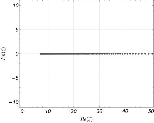
Figure 6: The poles of the Borel transform Eq. (60).

The attractor in HJSW hydrodynamics

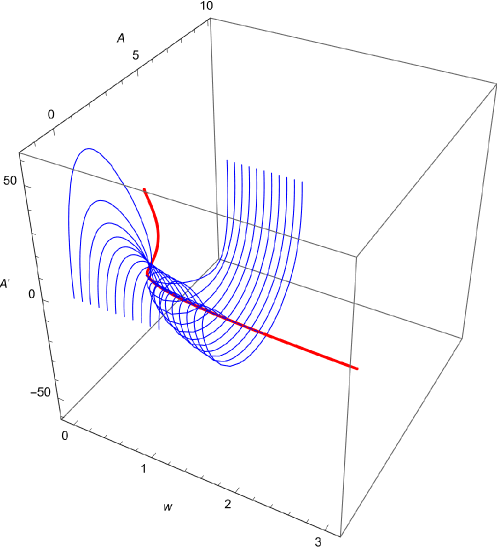
Figure 7: The blue curves depict solutions whose initial conditions were set at several values of $w$ between $0.05$ and $0.3$. The red curve represents the attractor. The parameter values used when making the plot were those for ${\mathcal{N}}=4$ SYM and $C_{\sigma}=0$.

So far this Section has focused on the attractor of MIS theory, but the same ideas can be applied to other hydrodynamic models discussed in Section 3. One point of interest is that in such models one sometimes encounters higher-dimensional phase spaces. For example, this happens in the HJSW model introduced in Ref. [54], which leads to a second order equation replacing Eq. (38). In consequence, the full phase space is three dimensional. Explicitly, this relaxation equation reads (see also Ref. [22])

$$\alpha_{1}\mathcal{A}^{\prime\prime}+\alpha_{2}\,\mathcal{A}^{\prime 2}+\alpha_{3}\,\mathcal{A}^{\prime}+12\,\mathcal{A}^{3}+\alpha_{4}\,\mathcal{A}^{2}+\alpha_{5}\,\mathcal{A}+\alpha_{6}=0,$$ (63)

where

$$\alpha_{1} = w^{2}\,(\mathcal{A}+12)^{2},$$

$$\alpha_{2} = w^{2}\,(\mathcal{A}+12),$$

$$\alpha_{3} = 12\,w\,(\mathcal{A}+12)\,(\mathcal{A}+3\,w\,\Omega_{I}),$$

$$\alpha_{4} = 48\,(3\,w\,\Omega_{I}-1),$$

$$\alpha_{5} = 108\,\left(-4\,C_{\eta}\,C_{\sigma}+3\,w^{2}\,\Omega^{2}\right),$$

$$\alpha_{6} = -864\,C_{\eta}\,\left(-2\,C_{\sigma}+3\,w\,\Omega^{2}\right).$$ (64)

At early times there is a unique power series solution regular at $w=0$:

$$\mathcal{A}(w)=4+\frac{54\,C_{\eta}\,|\Omega|^{2}-48\,\Omega_{I}}{20-9\,C_{\eta}\,C_{\sigma}}\,w+\dots$$ (65)

This is the attractor, as seen in Fig. 7, where this curve is plotted in the full phase space.

At large $w$, the gradient expansion takes the form

$$\mathcal{A}(w)=\frac{8C_{\eta}}{w}+\frac{16C_{\eta}(2\Omega_{I}-C_{\sigma})}{3|\Omega|^{2}w^{2}}+\dots$$ (66)

As expected, the first term captures the shear viscosity, as in MIS theory. The higher order terms differ from the corresponding expansion given in Eq. (47), (48). Similarly to the case of MIS theory, this series has vanishing radius of convergence [60]. One can use this expansion in conjunction with Borel summation to obtain a useful estimate of the attractor. We will return to this point in Section 6.

Attractors in general frame models

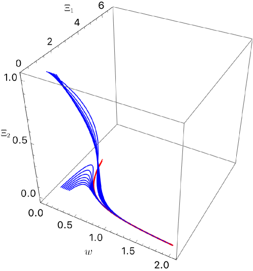
Figure 8: The blue curves depict solutions whose initial conditions were set at several values of $w$ between $0.05$ and $0.3$. The red curve represents the attractor. The parameter values used when making the plot were $C_{\eta}=0.08,C_{\tau}=0.2,C_{\varphi}=0.01$.

Attractors have also been studied in hydrodynamic models where the Landau frame condition has not been imposed [109, 20, 67, 110]. Here we wish to highlight an interesting example of an attractor within a $3$-dimensional phase space which arises in the general-frame MIS theory of Ref. [20] (see Section 3.6). Imposing the symmetries of Bjorken flow implies that the energy-momentum tensor contains three functions of proper time (instead of two, as would be the case had the Landau frame condition been imposed). This leads to a system of coupled equations for two functions of $w$, denoted by $\Xi_{1},\Xi_{2}$:

$$\frac{1}{12}(C_{\tau}-C_{\varphi})w(\Xi_{1}+12)\Xi_{1}^{\prime}-\frac{3}{8}w\Xi_{1}(\Xi_{2}-4)+\frac{(C_{\tau}-C_{\varphi})}{3}\Xi_{1}^{2}-\frac{9}{2}w\Xi_{2}-12C_{\eta} = 0,$$ (67)

$$\frac{1}{12}C_{\tau}w(\Xi_{1}+12)\Xi_{2}^{\prime}+\frac{1}{3}\Xi_{1}(C_{\tau}\Xi_{2}+C_{\varphi})+\frac{3}{2}w\Xi_{2} = 0,$$ (68)

where the prime denotes differentiation with respect to $w$, and $C_{\varphi},C_{\tau}$ are dimensionless constants. The functions $\Xi_{1},\Xi_{2}$ replace the pressure anisotropy in parametrising the dissipative part of the general-frame energy-momentum tensor and are defined in Ref. [20]. In the special case where $C_{\varphi}=0$ these equations admit a solution with $\Xi_{2}\equiv 0$ and then Eq. (67) reduces to the equation satisfied by the pressure anisotropy in MIS theory Eq. (38). The late time asymptotics of solutions are $\Xi_{1}\sim 8C_{\eta}/w$ and $\Xi_{2}\sim-63C_{\eta}C_{\varphi}/27w^{2}$ for all initial conditions.

The phase space of solutions in this model is three-dimensional rather than two-dimensional as in MIS theory. As in the examples discussed earlier, there is a unique solution regular at $w=0$ which acts as an attractor, as seen in Fig. 8.

Attractors from Kinetic Theory

The discovery of attractors in hydrodynamic models can be viewed as a strong indication that similar phenomena should occur also in more elaborate microscopic theories. This supposition has by now been confirmed in numerous studies discussed further in this review. The simplest class of models, whose complexity goes beyond what is discussed in the previous Section, are models of kinetic theory, where attractors have been identified and studied in many interesting cases [80, 21, 17, 111, 112, 113, 18, 114, 84, 85, 115, 78, 116, 19, 117, 118, 119, 93, 120, 121].

Kinetic theory is based on the classical notion of a single particle distribution function $f(x,p)$ obeying the Boltzmann equation

$$p^{\mu}\partial_{\mu}f(x,p)=\mathcal{C}[f]\leavevmode\nobreak\ .$$ (69)

The collision kernel appearing on the right-hand side of Eq. (69) can in general be very complicated, since in principle it should account for all scattering processes which can occur in a given theory. In practice, only a subset is accounted for, or some other form of approximation has to be adopted to capture essential features of the underlying microscopic theory. Here we will review kinetic theory attractors assuming one of two options: the relaxation time approximation (RTA) [122] and the Effective Kinetic Theory for Quantum Chromodynamics (EKT) [123].

Boost invariant flow in RTA

A significant simplification, which has been the subject of numerous studies is the relaxation time approximation, where the collision kernel in Eq. (69) is replaced by

$$\mathcal{C}[f]=p^{\mu}u_{\mu}\frac{f-f_{\rm eq}}{\tau_{R}}\leavevmode\nobreak\ .$$ (70)

Here $\tau_{R}$ is a momentum-independent relaxation time and $f_{\rm eq}=\exp\left(-\frac{p_{\mu}u^{\mu}}{T}\right)$ is the equilibrium distribution function. The resulting equation is linear in $f(x,p)$ and is much easier to work with. Recently, this ansatz has been generalised in various ways [124, 125, 126, 110, 127].

The Boltzmann equation in the RTA applied to Bjorken flow is a quasi-analytically solvable problem [128, 129] which provides a very useful environment for testing ideas of nonequilibrium dynamics. Since the one particle distribution function $f(x,p)$ is a scalar, boost invariance implies that it may depend only on variables invariant under longitudinal boosts: $\tau$, $p_{T}$, and $W=tp_{L}-zE$, where $E\equiv p_{0}=\sqrt{p_{T}^{2}+p_{L}^{2}+m^{2}}$ is the particle’s energy [130, 131] . With the help of $W$ one can define $v(p_{T},W,\tau)=Et-p_{L}z=\sqrt{W^{2}+(p_{T}^{2}+m^{2})\tau^{2}}\leavevmode\nobreak\ ,$ which allows us to express energy and longitudinal momentum of particles of mass $m$ in terms of boost-invariant variables

$$E=\frac{vt+Wz}{\tau^{2}}\leavevmode\nobreak\ ,\qquad p_{L}=\frac{Wt+vz}{\tau^{2}}\leavevmode\nobreak\ .$$ (71)

In terms of $\tau$, $W$ and $v$ we can write $p^{\mu}\partial_{\mu}f=\frac{v}{\tau}\partial_{\tau}f$, $p_{\mu}u^{\mu}=\frac{v}{\tau}$, and the boost-invariant Boltzmann equation in the RTA takes the form [18, 128, 129]

$$\partial_{\tau}f(\tau,W,p_{T})=\frac{f_{\rm eq}(\tau,W,p_{T})-f(\tau,W,p_{T})}{\tau_{R}}\leavevmode\nobreak\ .$$ (72)

The equilibrium distribution function is explicitly given by

$$f_{\rm eq}(\tau,W,p_{T})=\exp\left(-\beta u_{\mu}p^{\mu}\right)=\exp\left(-\frac{\sqrt{W^{2}+p_{T}^{2}\tau^{2}}}{T(\tau)\tau}\right)\leavevmode\nobreak\ ,$$ (73)

where we have set $m=0$, since for the time being we will concentrate on models respecting conformal symmetry.

In order to obtain a closed system of equations one needs a way to determine the effective temperature $T(\tau)$ appearing in Eq. (73). This can be achieved by imposing the Landau matching condition, which states that local energy density determined by the function $f(\tau,W,p_{T})$ should be equal to the equilibrium configuration with temperature $T(\tau)$. In order to do that in a Lorentz invariant way one uses the measure

$$dP=\frac{d^{4}p}{(2\pi)^{4}}2\pi\delta(p^{2})2\theta(p^{0})=\frac{dp_{L}}{(2\pi)^{3}p^{0}}d^{2}p_{T}=\frac{dWd^{2}p_{T}}{(2\pi)^{3}v}\leavevmode\nobreak\ ,$$ (74)

and the desired matching condition is expressed as

$$\mathcal{E}(\tau)=\int dP(p_{\mu}u^{\mu})^{2}f(\tau,W,p_{T})=\frac{3T(\tau)^{4}}{\pi^{2}}\leavevmode\nobreak\ .$$ (75)

A beautiful fact of life is that Eq. (72) admits the general solution [128, 129]

$$f(\tau,W,p_{T})=D(\tau,\tau_{0})f_{0}(W,p_{T})+\int_{\tau_{0}}^{\tau}\frac{d\tau^{\prime}}{\tau_{R}(\tau^{\prime})}D(\tau,\tau^{\prime})f_{\rm eq}(\tau^{\prime},W,p_{T})\leavevmode\nobreak\ ,$$ (76)

where $f_{0}(W,p_{T})$ is the initial distribution function at $\tau=\tau_{0}$, and $D(\tau_{2},\tau_{1})$ is given by

$$D(\tau_{2},\tau_{1})=\exp\left[-\int_{\tau_{1}}^{\tau_{2}}\frac{dt}{\tau_{R}(t)}\right]\leavevmode\nobreak\ .$$ (77)

The first term in Eq. (76) expresses free streaming, which dominates at early times, while the second term is captures relaxation toward local equilibrium, which is controlled by $\tau_{R}$.

The gradient expansion

The Boltzmann equation in the RTA Eq. (72) can be used to calculate the distribution function in the gradient expansion. The most direct way to proceed is to solve it iteratively starting with the equilibrium distribution, thus implementing the Chapman-Enskog expansion (see e.g. [132, 133]). One can then calculate the late proper time expansion of the effective temperature using Eq. (75) and translate it into a series for the pressure anisotropy, which can be written in the form of Eq. (47), with the leading coefficients given by [80]

$$a_{1}=\frac{8}{5}\ \gamma,\quad a_{2}=\frac{32}{105}\ \gamma^{2},\quad a_{3}=-\frac{416}{525}\,\gamma^{3}\leavevmode\nobreak\ .$$ (78)

This can be matched to the gradient expansion of any hydrodynamic model [96]. Depending on the choice of model, one or more terms may be matched. In the case of MIS theory, a comparison with Eq. (48) shows that to match RTA kinetic theory one needs $C_{\eta}=\gamma/5$.

The large order behaviour of the gradient expansion reveals a nonhydrodynamic mode with the expected relaxation time, but the results are actually much more complex, because of the wealth of possible initial conditions in kinetic theory, where the initial state is specified by the distribution function at some initial time. This will not be discussed further here, but some details can be found in Refs. [80, 112]. Note also that the spectrum of nonhydrodynamic modes in RTA kinetic theory is very different from that of hydrodynamic models [57].

The initial value problem

The additional input needed to evaluate Eq. (76) is an initial condition. An important example, used below, is the Romatschke-Strickland parametrisation [134]

$$f_{0}(W,p_{T})=\exp\left[-\frac{\sqrt{(p\cdot u)^{2}+\xi_{0}(z\cdot p)^{2}}}{\Lambda_{0}}\right]=\exp\left[-\frac{\sqrt{(1+\xi_{0})W^{2}+p_{T}^{2}\tau^{2}_{0}}}{\Lambda_{0}\tau_{0}}\right]\leavevmode\nobreak\ ,$$ (79)

where $-1<\xi_{0}<\infty$ measures initial momentum space anisotropy, $z_{\mu}=(\frac{z}{\tau},0,0,\frac{t}{\tau}),$ and $\Lambda_{0}$ determines the characteristic energy scale. Using this form, one can explicitly evaluate the initial energy density

$$\mathcal{E}(\tau_{0})=\int dP(p\cdot u)^{2}f_{0}(\tau_{0},W,p_{T})=\frac{3T_{0}^{4}}{\pi^{2}}\frac{\mathcal{H}(\frac{\alpha_{0}\tau_{0}}{\tau_{0}})}{\mathcal{H}(\alpha_{0})}\leavevmode\nobreak\ ,$$ (80)

where $\alpha_{0}=(1+\xi_{0})^{-\frac{1}{2}}$. Using the Landau matching condition, along with the general solution presented in Eq. (76) one then obtains an integral equation for the $T(\tau)$, i.e., the effective temperature as a function of proper time $\tau$ [128, 129]

$$T(\tau)^{4}=D(\tau,\tau_{0})T_{0}^{4}\frac{\mathcal{H}\left(\frac{\alpha_{0}\tau_{0}}{\tau}\right)}{\mathcal{H}(\alpha_{0})}+\int_{\tau_{0}}^{\tau}\frac{d\tau^{\prime}}{2\tau_{\rm eq}(\tau^{\prime})}D(\tau,\tau^{\prime})T(\tau^{\prime})^{4}\mathcal{H}\left(\frac{\tau^{\prime}}{\tau}\right)\leavevmode\nobreak\ ,$$ (81)

where

$$\mathcal{H}(y)=y\int_{0}^{\pi}\sin(\phi)\sqrt{y^{2}\cos^{2}(\phi)+\sin^{2}(\phi)}d\phi\leavevmode\nobreak\ .$$ (82)

Equation (81) can be solved in an iterative manner, with some initial temperature profile $T(\tau)$ [18]. Knowing the temperature as a function of $\tau$ one can carry out the integral in Eq. (76) to obtain the full distribution function $f(\tau,W,p_{T})$.

Attracting behaviour of the distribution function

To establish the existence of an attractor in kinetic theory one may adopt one of two approaches. The first is to look at the moments of the distribution function [21, 78, 85, 19] while the second looks for attractor behaviour of the distribution function itself [18]. In this subsection we will follow the latter approach, while the former will be described in Sec. 5.5 in the context of more realistic approximation to the collisional kernel [19].

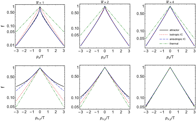
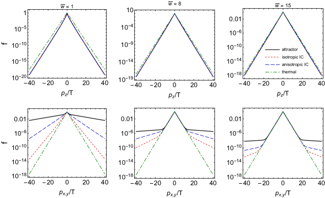
Figure 9: Quantitative approach towards a hydrodynamic attractor $\alpha_{0}\simeq 0.0025$ (solid black line) in the distribution function. Initial conditions are $T_{0}=1$ GeV at $\tau_{0}=0.1$ fm/c and $0.1\leq\alpha_{0}\leq 1.5$ for dashed/dotted colour lines. The first and third rows show $f(p_{T}=0,p_{L})$, while second and fourth show $f(p_{T},p_{L}=0)$. First two columns are for lower momenta $p_{i}/T\leq 3$ while second two columns are for higher momenta $p_{i}/T\leq 40$ ($i=x,y,z$). Different columns represent different time $\overline{w}$ instances marked in the top. The scaled variable $\overline{w}=\tau/\tau_{R}=\frac{\tau T(\tau)}{5\bar{\eta}}$, which differs by a constant factor from the variable $w=\tau T(\tau)$ introduced earlier. Plots from Ref. [18].

In order to demonstrate that the full distribution function $f(\tau,W,p_{T})$ has an attractor one numerically solves the RTA Boltzmann equation (72) for the class of initial conditions parametrised by Eq. (79) and identifies the attractor by a "slow roll" approximation [17, 18]:

$$\left.\mathcal{A}^{\prime}(\tau T)\right|_{\tau=\tau_{0}}\propto\left.\frac{\mathcal{E}\partial_{\tau}\mathcal{E}+\tau\mathcal{E}\partial^{2}_{\tau}\mathcal{E}-\tau(\partial_{\tau}\mathcal{E})^{2}}{\mathcal{E}^{2}}\right|_{\tau=\tau_{0}}\leavevmode\nobreak\ ,$$ (83)

with $T(\tau_{0})=1$ GeV and $\tau_{0}=0.1$ fm/c [18]. Solving $\mathcal{A}^{\prime}|_{\tau=\tau_{0}}=0$ for $\alpha_{0}$ singles out the value of the initial anisotropy parameter $\alpha_{0}\approx 0.0025$, which determines the attractor solution.

The approach to the attractor for different anisotropic initial configurations is shown in Fig. 9. It is apparent that the infrared part of the distribution function (the region close to $p=0$) approaches the attractor earlier than the ultraviolet part, which is a manifestation of the “bottom-up” scenario characteristic of weakly coupled systems [33]. The approach to the attractor is also slower in the transverse direction ($p_{z}=0$) than in the longitudinal direction ($p_{T}=0$). Note also that in some momentum regions the attractor is approached from below, while in others it is approached from above.

Weakly coupled QCD

The discussion of previous section relied on the RTA collisional kernel. An important question is whether similar results can be established within more realistic models. Recently, this issue was addressed in the context of Effective Kinetic Theory (ETK) of QCD [123]. The EKT Boltzmann equation for a pure gluon system reads

$$-\partial_{\tau}f+\frac{p_{z}}{\tau}\partial_{p_{z}}f=\mathcal{C}_{1\leftrightarrow 2}[f]+\mathcal{C}_{2\leftrightarrow 2}[f]\leavevmode\nobreak\ ,$$ (84)

where the inelastic $\mathcal{C}_{1\leftrightarrow 2}$ and elastic $\mathcal{C}_{2\leftrightarrow 2}$ collisional terms include physics of dynamical screening and Landau-Pomaranchuk-Migdal damping. Although EKT is does not account for the full complexity of QCD, for isotropic systems it incorporates the leading $\alpha_{s}$-order description and has been extensively used to address off-equilibrium perturbative QGP dynamics [135, 136, 137].

To study the process of equilibration, Ref. [19] considers the set of moments of the distribution functions defined by

$$\mathcal{M}^{nm}(\tau):=\int\frac{d^{3}p}{(2\pi)^{3}}p^{n-1}p_{z}^{2m}f(\tau,\bf p)\leavevmode\nobreak\ ,$$ (85)

where $p=|{\bf p}|$. In terms of these, the energy density of a massless particle gas is $\mathcal{E}=\mathcal{M}^{20}$, particle density is $n=\mathcal{M}^{10}$, while the longitudinal pressure reads $P_{L}=\mathcal{M}^{01}$. The pressure anisotropy can be expressed in terms of these moments as

$$\mathcal{A}=3\frac{\mathcal{P}_{T}(\tau)-\mathcal{P}_{L}(\tau)}{\mathcal{E}(\tau)}=\frac{3}{2}-\frac{9}{2}\frac{\mathcal{M}^{01}(\tau)}{\mathcal{M}^{20}(\tau)}\leavevmode\nobreak\ .$$ (86)

The distribution function can be obtained numerically by solving the Boltzmann equation (84) utilising the algorithm described in Ref. [138, 135].

Two classes of initial conditions were considered in Ref. [19]. The first one is given by a spheroidally deformed thermal distribution function given by

$$f_{0,\rm RS}(p)=\frac{1}{\exp\left(\frac{\sqrt{p^{2}+\xi_{0}^{2}p_{z}^{2}}}{\Lambda_{0}}\right)-1},$$ (87)

where $-1<\xi_{0}<\infty$, as in the RTA case, parametrises the initial momentum anisotropy, while $\Lambda_{0}$ sets the initial energy scale. The second group of initial conditions is given by the non-thermal CGC-motivated distribution function, explicitly written as

$$f_{0,\rm CGC}(p)=\frac{2A}{\lambda_{\rm YM}}\frac{Q_{0}}{\sqrt{p^{2}+\xi_{0}^{2}p_{z}^{2}}}\exp\left(-\frac{2}{3}\frac{p^{2}+\xi_{0}^{2}p_{z}^{2}}{Q_{0}^{2}}\right)\leavevmode\nobreak\ ,$$ (88)

where the scale $Q_{0}$ is related to the QCD saturation scale $Q_{0}=\langle p_{T}\rangle_{0}\approx 1.8Q_{s}$ [139]. Furthermore, $\lambda_{\rm YM}=g_{\rm YM}^{2}N_{c}$ is the ’t Hooft coupling. The normalisation constant $A$ is fixed by matching the initial energy density with the predictions of classical Yang-Mills theory $\tau_{0}\mathcal{E}_{0}=0.358\nu_{\rm eff}\frac{Q_{s}^{3}}{\lambda_{\rm YM}}$ [140]. For both sets of initial conditions, the scales $\Lambda_{0}$ and $Q_{0}$ play a role similar to the temperature in a thermal distribution, i.e., they determine which portion of momentum space is occupied. The fact that distribution in Eq. (88) is inversely proportional to $\lambda_{\rm YM}$ reflects the overpopulation of gluons determined by multiple low energy scatterings at initial times.

The plots in Fig. 10 show the evolution of three sample moments with different initial conditions, parametrised by Eq. (87) and Eq. (88). As seen in the upper panel of Fig. 10, all sampled initial conditions merge into one universal line, the hydrodynamic attractor, before they are well approximated by the viscous hydrodynamics. This happens on the time scale $\tau/\tau_{R}\sim 0.5$ common for all three moments of the distribution function. Since this result holds also for higher moments, it is a strong indication that, similarly to the RTA case, the attractor is present in the full one particle distribution function [141].

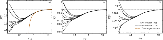
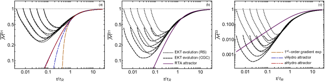
Figure 10: Evolution of the scaled moments $\overline{\mathcal{M}}^{nm}(\tau)=\mathcal{M}^{nm}(\tau)/\mathcal{M}^{nm}_{\rm eq}(\tau)$ computed as functions of rescaled time $\overline{w}=\tau/\tau_{R}=\frac{\tau T(\tau)}{5\bar{\eta}}$ for various initial conditions. Upper panel: fixed initial time different initial momentum space anisotropy. Lower panel: different initial times with fixed initial momentum anisotropy. The value the ’t Hooft coupling used here is $\lambda_{\rm YM}=10$, which corresponds to shear viscosity $\eta/s\approx 0.63$ [142, 143]. The plots are taken from Ref. [19].

The plots in the lower panel of Fig. 10 show evolution of moments initialised at successively smaller initial times $\tau_{0}$. As apparent from the figure, earlier initialisation leads to faster decay to the attractor, suggesting a scaling dependence on $\tau_{0}$ at early times. At late times, both RS and CGC initial conditions follow the same attractor, showing that details of hydrodynamic evolution are insensitive not only to the initial pressure anisotropy but also to microscopic features such as momentum distribution and initial occupancy. While true at late times, this need not be the case at very early times where different models predict different attractors, as also indicated in Fig. 10. This will be discussed further in Section 8.

Attractor behaviour through AdS/CFT

In this Section we review studies of equilibration of Bjorken flow in ${\mathcal{N}}=4$ SYM theory, which are possible to carry out in the strong coupling limit by virtue of the AdS/CFT correspondence [144, 145]. Excellent reviews of the applications of holographic methods to heavy ion collisions include Refs. [146, 147, 148, 149]; applications to Bjorken flow are reviewed in Refs. [150, 22, 23, 24]. In this Section we will therefore refrain from discussing the techniques involved, our focus being on the results of such calculations and their interpretation in terms of hydrodynamic attractors.

Thermal states in AdS/CFT

The basic fact which lies at the heart of applying AdS/CFT to nonequilibrium physics is that the equilibrium state of ${\mathcal{N}}=4$ supersymmetric Yang-Mills plasma in $4$-dimensional Minkowski space corresponds to a black hole in asymptotically-$AdS_{5}$ space. This object is often referred to as a black brane due to the fact that the horizon of the gravitational solution is planar rather than spherical. The black brane temperature $T$ is equal to the temperature of the plasma. The duality map (sometimes referred to as the holographic dictionary) leads to a formula for the energy density of the plasma:

$$\mathcal{E}=\frac{3\pi^{2}}{8}N_{c}^{2}T^{4}.$$ (89)

Up to a factor of $3/4$, which is interpreted as the effect of strong coupling, this coincides with the result for the energy density of quanta comprising the plasma in the absence of interactions.

The interpretation of the equilibrium state in terms of a black hole immediately suggests that its perturbations should correspond to perturbations of the black hole. Their spectrum can therefore be computed by standard methods developed in studies of general relativity, adapted to the specific challenges of asymptotically AdS spaces. At the linearised level such perturbations are known as quasinormal modes (QNM) of the black hole, and they describe damped oscillations of the black hole horizon. Their complex frequencies naturally fall into one of two categories: a finite number of hydrodynamic modes whose damping rate is proportional to the wave vector, and an infinite series of nonhydrodynamic modes which are damped even for arbitrarily long-wavelength perturbations. This matches directly the picture of perturbations of equilibrium expected on the basis of linear response theory, as reviewed in Section 3.4.

The process of equilibration can also be described analytically at the nonlinear level. This was pioneered in Refs. [151, 152, 153, 154] by studies of the asymptotic late-time expansion of Bjorken flow (reviewed in Section 6.3 below). These results were subsequently generalised to generic near-equilibrium states [46], which are mapped to perturbed black objects in asymptotically $AdS$ spaces described in a gradient expansion analogous to what is done in hydrodynamics. This connection is sometimes referred to as the fluid-gravity correspondence. It has also led to an interpretation of off-equilibrium entropy in field theory in terms of slowly-evolving horizons in the dual gravitational representation [155, 156, 157]. These analytic studies have provided a number of insights which were later applied to numerical simulations and have greatly aided the interpretation of their results.

Numerical solutions and early time behaviour

Numerical approaches to solving the initial value problem in the gravitational representation of Bjorken flow and translating the result into field theory language have also been critically important [158, 159, 160, 161, 162, 163]. One of the first steps in such calculations is the selection of consistent initial geometries. This is a nontrivial task, as it requires satisfying the constraints following from Einstein equations. A basic result is that the early-time behaviour of the energy density on the field theory side has the form of a Taylor series with only even powers of the proper time [164]:

$$\mathcal{E}=\mathcal{E}_{0}+\mathcal{E}_{2}\tau^{2}+O(\tau^{4})\leavevmode\nobreak\ .$$ (90)

In Refs. [160, 161, 163] the initial conditions were set in such a way that the leading coefficient $\mathcal{E}_{0}\neq 0$. This corresponds to the initial value of the pressure anisotropy $\mathcal{A}(0)=6$. A number of such solutions are plotted in Fig. 11. It is apparent that the pressure anisotropy reaches the hydrodynamic attractor while the system is still very anisotropic. It is not clear however whether an expansion dominated regime exists at early times. This is partly due to the oscillatory behaviour, which is interpreted as a consequence of the rich spectrum of nonhydrodynamic modes whose frequencies are not purely imaginary, in contrast to models of MIS hydrodynamics or kinetic theory. A possibly more significant issue is that the effective phase space of the theory is multidimensional. While two real numbers suffice to specify the initial data for the equations for Bjorken flow in MIS theory, in the AdS/CFT calculation the initial data is specified by a function of the radial (holographic) coordinate in the asymptotically-AdS space, which defines the initial geometry. If this were coarse-grained in some way, one could represent the phase space as a having effectively a finite number of dimensions, but there is no reason to believe that a two-dimensional truncation would provide a reasonable account. The plot of $\mathcal{A}(w)$ should therefore be viewed as a projection from a high-dimensional phase space and may obscure the picture at early times. An indication of this can be seen in Fig. 7 and 8.

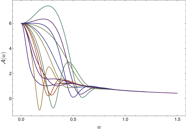
Figure 11: Pressure anisotropy as a function of $w$ for $\mathcal{N}=4$ SYM at strong coupling [165].

In contrast with hydrodynamic models, where a regular solution at $w=0$ was a natural candidate for an attractor, there is no such natural candidate here. In Ref. [36] an attempt was made to find a physical argument which would single out a special initial condition close to $w=0$. An interesting feature of this proposed attractor is that it appears to be close to free-streaming at early times, just as what is found in kinetic theory. A somewhat complementary approach to identifying the early-time attractor based on Borel summation of the gradient expansion is also not conclusive, since it looses predictivity at very early times, as reviewed in Section 6.4 below.

The existence of an early-time attractor in this theory is of great interest, and this question was revisited recently in Ref. [78]. In this paper the authors looked for the early, expansion-dominated phase and did not find evidence for it. The evolution of the pressure anisotropy for a number of solutions is shown in Fig. 12, where it is apparent that the approach to the attractor is determined by the $1/T$ scale irrespective of the initialization time.

In summary, the status of the early-time attractor in the case of ${\mathcal{N}}=4$ SYM is not entirely clear at this time. It is expected to exist on the basis of general, kinematic arguments, but it could also be that due to the strong coupling limit the expansion dominated region is artificially smeared out and effectively only a late time attractor exists.

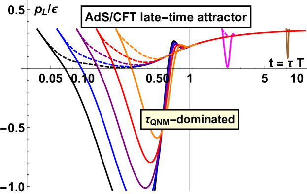
Figure 12: Evolution of various initial configurations in holography. Note that the pressure anisotropy is connected to the quantity in the plot through the relation $\mathcal{A}=-\frac{3}{2}+\frac{9P_{L}}{2\epsilon}$. Plot form Ref. [78].

The large proper time expansion

The emergence of fluid behaviour in boost-invariant ${\mathcal{N}}=4$ SYM was first demonstrated in Refs. [151] by studying the behaviour of the energy density at large values of the proper time. The asymptotic behaviour of the energy density is given by

$$\mathcal{E}_{\rm hydro}(\tau)\sim\frac{\Lambda^{4}}{(\Lambda\tau)^{4/3}}{\sum_{n=0}^{\infty}\mathcal{E}_{n}^{(0)}(\Lambda\tau)^{-2n/3}}\leavevmode\nobreak\ ,$$ (91)

where the energy scale $\Lambda$ reflects the initial conditions, as in other cases of Bjorken flow, and $\mathcal{E}_{0}^{(0)}=1$. The expansion coefficients $\mathcal{E}_{n}^{(0)},n>0$ can be determined using the AdS/CFT correspondence. The first three subleading orders were calculated analytically [152, 154, 166], and higher orders numerically [94, 167]. For $n\gg 1$ these coefficients diverge factorially, i.e.

$$\mathcal{E}_{n}^{(0)}\sim\frac{\Gamma(n+\beta_{1})}{A_{1}^{n+\beta}}+{\rm h.c.}\leavevmode\nobreak\$$ (92)

where $A_{1},\beta_{1}$ are complex constants; the singulant $A_{1}$ turns out to be related to the lowest nonhydrodynamic quasinormal mode frequency of the dual black hole $\omega_{1}=3.1195-{\rm i}2.7467$ [168] by the relation $A_{1}={\rm i}\frac{3}{2}\omega_{1}$. This connection of large order behaviour of the gradient expansion to the nonhydrodynamic modes is therefore fully analogous to what was discussed in Section 4.8 in the case of MIS theory.

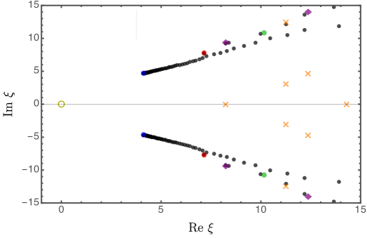
Figure 13: Poles of the Borel-Padé approximant $\mathrm{BP}_{189}\left[\mathcal{E}_{\rm hydro}\right]$, in the complex $\xi-$plane. We can see the appearance of the different fundamental sectors (shown as filled circles) as well as mixed sectors (shown as filled purple diamonds). The predicted branch points for each sector are marked by colours: $A_{1}$ and $\overline{A_{1}}$ (blue), $A_{2}$ and $\overline{A_{2}}$ (red), $A_{3}$ and $\overline{A_{3}}$ (green). This plot is taken from Ref. [167].

Equation (91) cannot be the whole story, since initial states in $AdS$ contain much more information than just the scale $\Lambda$. In fact, each nonhydrodynamic mode of ${\mathcal{N}}=4$ SYM plasma introduces an exponentially damped transseries sector, with an independent transseries parameter which corresponds to a piece of initial data. Thus, the full expansion of $\mathcal{E}(\tau)$ takes form of multi-parameter transseries with infinitely many transseries parameters [167]:

$$\mathcal{E}(\tau)\sim\underbrace{\frac{\Lambda^{4}}{(\Lambda\tau)^{4/3}}{\sum_{n=0}^{\infty}\mathcal{E}_{n}^{(0)}(\Lambda\tau)^{-2n/3}}}_{\mathcal{E}_{\rm hydro}(\tau)}+\frac{\Lambda^{4}{\sigma_{1}}}{(\Lambda\tau)^{4/3}}{\sum_{n=0}^{\infty}\mathcal{E}_{n}^{(1)}(\Lambda\tau)^{-2n/3}e^{-A_{1}(\Lambda\tau)^{2/3}}}+{\rm h.c.}+\cdots$$ (93)

For simplicity, only one nontrivial transseries sector is written explicitly in Eq. (93); it is the contribution of the least-damped, transient mode determined by the complex quasinormal mode frequency $A_{1}$. The imaginary part of $A_{1}$ controls the exponential damping, while the real part determines the oscillation frequency. The full solution also includes supplementary sectors representing mutual couplings between distinct modes. This intricate structure is reflected in Fig. 13, where the branch points correspond to quasinormal modes (as well as their products) [167].

All the coefficients $\mathcal{E}_{n}^{(k)}$ appearing in the transseries expansion in Eq. (93) can be determined using the AdS/CFT correspondence; many of them have been calculated numerically for the most relevant sectors in Ref. [167]. The original hydrodynamics series $\mathcal{E}_{n}^{(0)}$ diverges factorially, as in Eq. (92), and so do the series appearing in each transseries sector. For instance, in the first sector one finds that for $n\gg 1$

$$\mathcal{E}_{n}^{(1)}\sim\frac{\Gamma(n+\beta_{2})}{A_{2}^{n+\beta_{2}}}+\mathrm{h.c.}$$ (94)

where $A_{2},\beta_{2}$ are complex constants; the singulant $A_{2}={\rm i}\frac{3}{2}\omega_{2}$, where $\omega_{2}=5.1695-{\rm i}4.7636$ is second least damped QNM in the sense that $|{\rm Im}\ A_{1}|<|{\rm Im}\ A_{2}|$. This type of relation between series appearing in different transseries sectors is a manifestation of resurgence [107, 108]. The resurgence property of the transseries implies that the complete structure of the nonhydrodynamic sectors can be recovered from the original hydrodynamic gradient expansion.

The attractor by Borel summation

As reviewed in Section 4, one can estimate the location of the attractor by Borel summation of the hydrodynamic gradient expansion. To do this in the present case one has to calculate the expansion of the pressure anisotropy in powers of the $w$ variable using Eq. (91). This series is also factorially divergent and the analytic continuation of the Borel transform has the same pattern of singularities as seen in Fig. 13. In particular, there are no singularities on the real axis. This means that the Borel sum of this series does not suffer from the complex ambiguity encountered in the case of MIS theory. Of course the transseries contributions are still present, and will become significant for values of $w$ sufficiently far from the asymptotic region. Thus, at small values of $w$ this approach looses predictability, since the no longer negligible exponentially suppressed contributions eventually bring in dependence on the transseries coefficients and it is not known which values correspond to the attractor.

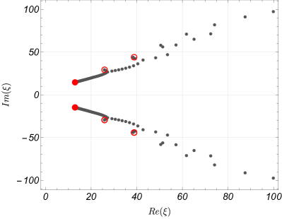
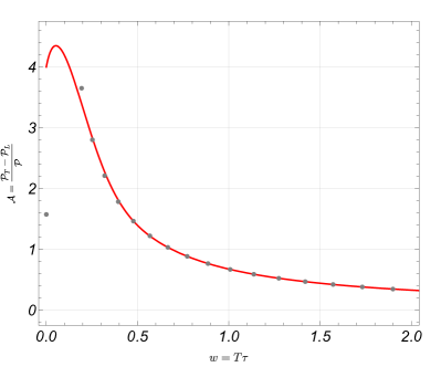
Figure 14: Left panel: poles of the Borel transform of the gradient series of HJSW hydrodynamics; the red dots represent the known complex frequencies $\Omega$ of the nonhydrodynamic modes; the circles show the locations of their multiples. Right panel: the numerical attractor in HJSW hydrodynamics projected on the $(w,\mathcal{A})$ plane (red curve) compared with the result of Borel summation of the gradient expansion (black dots).

This procedure has been in tested in the case of the HJSW model [54] which has a similar singularity structure and where the true attractor is easily found numerically. The relevant equation which is satisfied by $\mathcal{A}(w)$ is Eq. (63), which can easily be solved in a power series for large $w$; the leading terms appear in Eq. (66). This series is factorially divergent and the singularities of the analytic continuation of its Borel transform resemble those of ${\mathcal{N}}=4$ SYM, as seen in the right panel of Fig. 14. The series can then be Borel-resummed at various values of $w$ following the procedure outlined in Section 4.8. We can interpret the outcome as an approximation to the attractor. As seen from Fig. 14, the result is in excellent agreement with the numerical attractor down to $w\approx 0.4$. At earlier times the transient transseries contributions are no longer negligible. Moreover, these effects depend on the transseries parameters, and it is not known how to determine their values so as to reproduce the attractor. This would require connecting the late-time transseries with the convergent series describing the attractor Eq. (65). The analogous issue was recently discussed in MIS theory using transasymptotic summation [79], so perhaps this point could be addressed in the future.

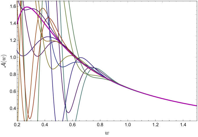
Figure 15: The pressure anisotropy as a function of $w$ for $\mathcal{N}=4$ SYM at strong coupling, along with the parametrized attractor (thick magenta line), from Eq. (95).

In the case of ${\mathcal{N}}=4$ SYM theory one can apply Borel summation to the gradient expansion in exactly the same way [169]. The resulting estimate of the attractor can be represented by fitting the numerical result to a rational function:

$$A_{\rm attr}(w)=\frac{-276w+2530}{3975w^{2}-570w+120}\leavevmode\nobreak\ .$$ (95)

It is apparent from Fig. 15 that this resummation breaks down below $w\approx 0.4$ and therefore sheds little light on the early-time behaviour.

To conclude this section, let us mention some results concerning finite coupling corrections [170]. Such corrections can be included by modifying the dual gravitational representation of the leading approximation discussed so far. The ensuing Bjorken flow gradient expansion can also be calculated to high order. The analytic continuation of its Borel transform reveals an interesting structure of singularities which interpolates between the one found in at infinite coupling [167] and the one familiar from kinetic theory [80].

The phase space perspective

We have seen that some part of the information about the initial state becomes suppressed during dissipative evolution. In the case of Bjorken flow this is especially clearly visible in the behaviour of $\mathcal{A}(w)$, where at late times the approach to equilibrium is independent of initial conditions up to exponentially suppressed corrections. Furthermore, in this case the attractor locus is one dimensional, and is in fact a solution of a differential equation. These features are a consequence of expressing the dynamics through a set of convenient variables. To explore hydrodynamic attractors beyond the simplest settings one needs to understand how to analyse the problem without such special variables, because in more complicated situations such variables may not be known, or even exist. In this Section we review a very general approach, which does not rely on any symmetry assumptions such as those of Bjorken flow [117]. It addresses the emergence of attractors by considering the behaviour multiple solutions in a suitably defined phase space. It is worth emphasising that this perspective can be applied to any dynamical model of equilibration, including models formulated in the language of kinetic theory and the AdS/CFT correspondence.

Dimensionality reduction

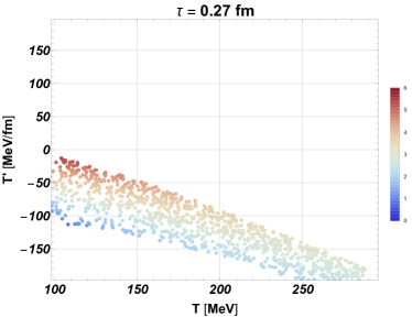
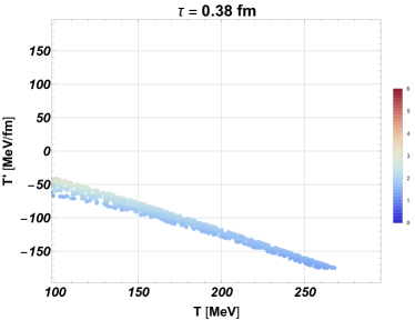
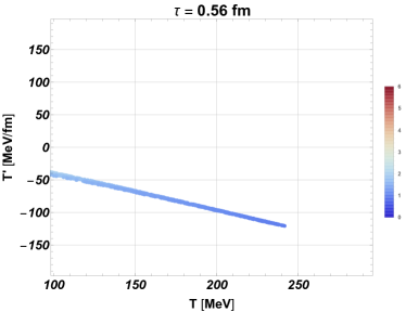
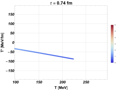
Figure 16: A sequence of snapshots expressing the evolution of a point-cloud of solutions plotted on a proper-time slice in boost-invariant MIS theory. Initially the depicted region is uniformly filled, but in subsequent plots we see the dimensionality reduced from $2$ to $1$. The colour of a dot encodes the effective temperature [171].

To introduce the basic idea we return to the simplest models of equilibration, formulated in the language of hydrodynamics. Given an equation such as Eq. (35), the most generic parametrisation of phase space would be to use $T(\tau),\dot{T}(\tau)$. The late time behaviour of the temperature Eq. (36) shows that any set of solutions whose initial conditions are set on some proper-time slice $\tau=\tau_{0}$, in the course of evolution collapses approximately onto a one-dimensional locus: a curve parametrised by the value of $\Lambda$, which is the only remnant of the initial state. In the simplest MIS model this means that only one combination of two integration constants is still accessible at late times, but in more complex models the initial state could carry much more information which is effectively dissipated by the time the asymptotic form Eq. (36) is reached. This suggests that even in more general settings one may view the attractor as a locus of low dimensionality embedded in a potentially high-dimensional phase space. One can thus say that evolution toward the hydrodynamic attractor is tantamount to dimensionality reduction of sets of solutions viewed on phase space slices.

We illustrate this perspective by considering the full phase space for Bjorken flow in MIS theory, parametrised by $(\tau,T,\dot{T})$ – the proper time is included as one of the phase space variables because equations of motion Eq. (35) depend explicitly on $\tau$. The plots in Fig. 16 allow us to follow a collection of solutions starting with a uniformly-distributed set of points on an initial proper-time slice. In the course of dissipative evolution one sees them all approaching the attractor locus, which in this case is a straight line, whose alignment depends on $\tau$.

Machine learning

The notion of dimensionality reduction in phase space is a promising perspective on hydrodynamic attractors, one which is not tied to the simplicity of Bjorken flow. A key element of this approach is some convenient, but essentially arbitrary parametrisation of phase space. In situations more generic than Bjorken flow this will certainly involve some coarse-graining, but one will still need to consider phase spaces of large dimensionality. This suggests applying machine learning techniques to this problem. This has not yet been fully explored in the published literature, but some encouraging pilot studies exist. Here we will comment briefly on the approach suggested in Ref. [117], which made use of one of the simplest dimensionality-reduction methods – Principal Component Analysis (PCA). PCA analyses the variations in a data set in different directions and associates an explained variance with each of them. In this way the number of principal components of a set of solutions on a proper time slice reflects the effective dimensionality of this point cloud. In the case of Bjorken flow, when the system is close to equilibrium this cloud will be one-dimensional, reflecting the single integration constant of the asymptotic Bjorken solution Eq. (9).

As a simple illustration, we begin by applying PCA to the two-dimensional phase space of MIS theory, so as to quantify the pattern of behaviour seen in Fig. 16. On the initial time slice we pick a state $(T,\dot{T})$ and consider a random set of points within a disc around it. For this set of points, the two principal components are approximately equal in magnitude. At each time step we recompute the principal components of this evolving point cloud; their evolution is shown in Fig. 17. Dimensionality reduction is signalled when one of the components is much smaller than the other one. It is significant that the dimensionality reduction splits into two stages: the first one can interpret as the effect of the longitudinal expansion, and the second as nonhydrodynamic mode decay.

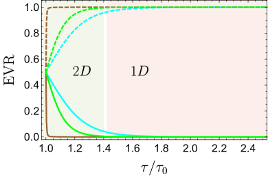
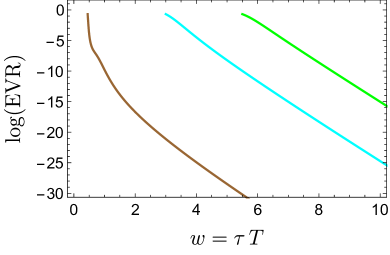
Figure 17: Left: evolution of explained variance ratio of each principal component in MIS/BRSSS for circles (radius: $10^{-4}$) of initial conditions with centres lying in the middle of initial dots of corresponding colour in Fig. 19. Right: logarithm of decaying principal components plotted as a function of $w$. For large enough values of $w$ one clearly sees persistent exponential decay. Plot from Ref. [117].

A similar picture emerges in the case of the HJSW model discussed in Section 3.5, where the phase space s three-dimensional. In this case the dimensionality reduction is even more striking, as seen in Fig. 18, whose bottom panel depicts three stages in the evolution of a uniform cloud of solutions at three instances of proper time. Initially, the boost-invariant expansion leads to a rapid, parameter-independent collapse of the three-dimensional region to a two-dimensional locus – this is the early-time, expansion-dominated phase. Subsequently the reduced two-dimensional cloud evolves until it shrinks to a line, as it must for conformal Bjorken flow. The dynamics of the second and third stages depend on the parameter values, as expected on the basis of the interpretation in terms of nonhydrodynamic mode decay. The evolution of principal components is shown in the upper part of Fig. 18, where one can clearly discern the three different stages with different dimensionality.

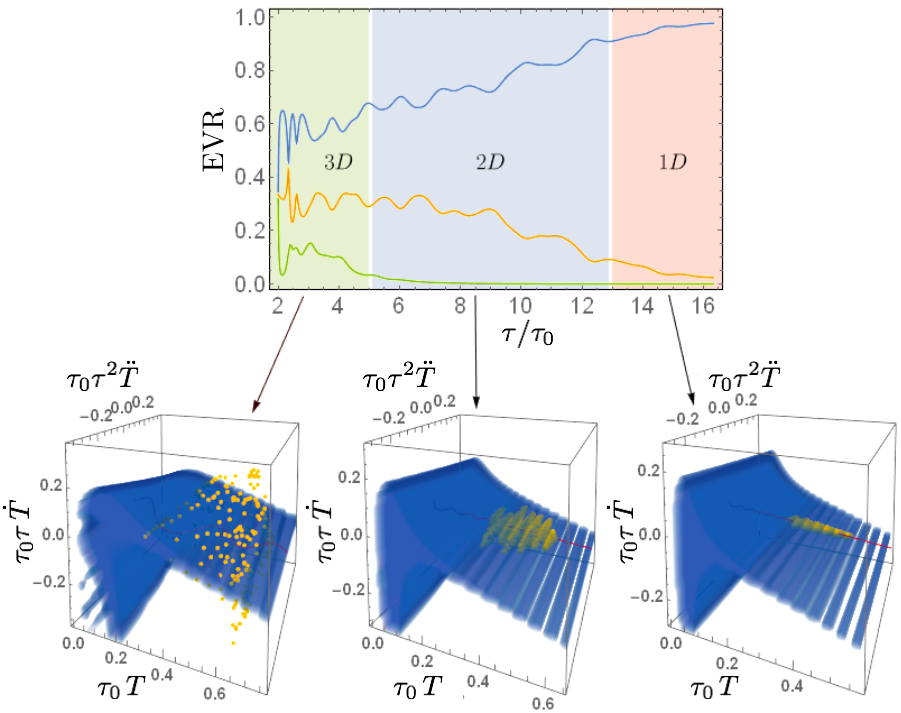
Figure 18: In the HJSW model, the evolution of a cloud in phase space can be split into three stages, corresponding to the dimensionality of the cloud. The reduction from three to two dimensions corresponds to a collapse onto the slow region (blue region in plots). Figure performed with $C_{\eta}=0.75$, $C_{\tau_{\pi}}=1.19$, and $C_{\omega}=9.8$, taken from Ref. [117].

This type of analysis can be applied to phase spaces of arbitrary dimensionality, in any dynamical model. This will in general involve some coarse graining and truncation of the phase space, which in itself need to be finite-dimensional. An enlightening example which illustrates these issues is provided by a model of Bjorken flow in kinetic theory in the RTA which can be found in the Supplemental Material of Ref. [117]. A more realistic study of the phase space approach to Bjorken flow in the effective kinetic theory of QCD can be found in Ref. [172]. These studies rely on PCA, but a number of other machine learning techniques exist which may provide a more refined picture, such as Topological Data Analysis (see e.g. [173]) which has recently been explored in a somewhat related physical context [174].

The attractor as a slow region

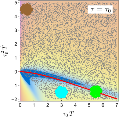
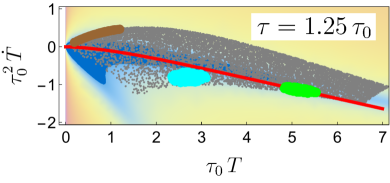
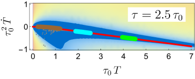
Figure 19: Three proper time slices of phase space tracking a cloud of about 10,000 solutions of MIS theory. The red curve denotes the attractor locus ${\cal A}_{\star}$. The background colour encodes the speed at which the points move in phase space, with magenta faster than blue according to the norm of velocity vector (96); the dark blue denotes the slow region. The plots were made for $C_{\eta}=0.75$ and $C_{\tau_{\pi}}=1$; $\tau_{0}$ denotes the initialisation time. Plot from Ref. [117].

In models with phase spaces whose dimension is greater than two, the attractor is not a single solution but rather a region of phase space onto which actual solutions condense. In conformal examples of Bjorken flow it was possible to project this region onto a single solution in the $\mathcal{A},w$ variables, but this is not expected to be possible in more general situations. Therefore, a more general characterisation of the attractor is needed. Intuitively one would expect that the attractor locus should correspond to a “slow region” where the flow in phase space is slowest, because it takes a long time to escape it, while the fast regions can be quickly traversed.

In the case of MIS this idea correctly identifies the attractor on any given proper time slice. A point on such a slice of phase space can be described by the vector $\vec{X}(\tau)=\left(\tau_{0}\,T(\tau),\tau_{0}^{2}\,\dot{T}(\tau)\right)$; its velocity is given by

$$\vec{V}=\tau_{0}\frac{\partial\vec{X}}{\partial\tau}\leavevmode\nobreak\ ,$$ (96)

where the factors of $\tau_{0}$ have been introduced for dimensional reasons. The slow region can be defined by the Euclidean norm $V$ of this vector, which has a minimum at asymptotically late times when the system approaches local thermal equilibrium. The resulting picture can be seen in Fig. 19; the background colour is determined by $V$, where bluer colour implies lower speed. There is a slow region stretching out from local thermal equilibrium, and the attractor $\mathcal{A}_{*}(w)$ lies along it. The identification of the attractor as a slow region at least in principle generalises directly to phase spaces of any dimension.

Attractors and prehydrodynamic flow

As discussed in Sec. 2, the standard picture of heavy-ion collisions involves formation of QGP followed by a stage of nonequilibrium evolution until a time when conventional fluid dynamics can be applied. The developments reviewed in the last four Sections suggest that approximate Bjorken symmetry of the early time dynamics could be responsible for a far-from-equilibrium attractor capable of providing a bridge between these two stages. This attractor could then be modelled using some much simpler effective description such as MIS theory used outside its naive domain of applicability. In this Section we will review some efforts aiming to apply this idea to QGP dynamics [175, 176]. Other work which makes practical use of attractors in the context of heavy-ion collisions includes Refs. [136, 137, 172, 177, 178, 179, 180, 181, 182, 183, 184, 185].

As currently understood (see Section 4), the existence of a nonequilibrium hydrodynamic attractor in Bjorken flow is contingent upon there being a definite, finite, physically distinguished value ${\mathcal{A}_{\star}}(0)$ of the pressure anisotropy at $w=0$ [14, 60]. One can translate this into a statement about the early time behaviour of the energy density. Indeed, under the above assumptions, the conservation of energy-momentum Eq. (7) implies that for asymptotically small proper-time $\tau$

$$\mathcal{E}\sim\frac{\mu^{4}}{(\mu\tau)^{\beta}}\leavevmode\nobreak\ ,$$ (97)

where the scale $\mu$ is an integration constant which reflects the initial conditions, and the exponent $\beta$ is related to the attractor by the relation

$${\mathcal{A}_{\star}}(0)=6\left(1-\frac{3}{4}\beta\right)\leavevmode\nobreak\ .$$ (98)

We will consider $0\leq\beta<4$ (where $\beta=1$ corresponds to free streaming). While different initial conditions will correspond to different values of $\mu$, the parameter $\beta$ characterises the attractor itself and is therefore a feature of the particular microscopic theory under consideration. For instance, in MIS theory the attractor is the unique stable solution which is regular at $w=0$, where

$${\mathcal{A}_{\star}}(0)=6\sqrt{\frac{C_{\eta}}{C_{\tau\Pi}}}\iff\beta=\frac{4}{3}\left(1-\sqrt{\frac{C_{\eta}}{C_{\tau\Pi}}}\right)\leavevmode\nobreak\ .$$ (99)

Entropy and particle production

The hydrodynamic attractor connects early and late-time behaviour of the system, and this fact makes it possible to relate final state entropy to characteristics of the initial state. We will denote the value of $w$ at very early proper time $\tau_{0}$ by $w_{0}$, and its value at late times $\tau_{\infty}$ by $w_{\infty}$. Since at late times the system is approaching thermal equilibrium, one may use standard thermodynamic relations to write the entropy density as

$$s(\tau_{\infty})=\frac{4}{3}\frac{\mathcal{E}(\tau_{\infty})}{T(\tau_{\infty})}$$ (100)

and then apply Eq. (41) to express the right hand side in terms of quantities evaluated at proper time $\tau_{0}$. This leads to the key relation between the entropy density per unit rapidity at late time and the initial energy density

$$s(\tau_{\infty})\tau_{\infty}=h(\beta)\left(\mathcal{E}(\tau_{0})\tau_{0}^{\beta}\right)^{\frac{2}{4-\beta}}\leavevmode\nobreak\ ,$$ (101)

where

$$h(\beta)=\frac{4}{3}w_{\infty}w_{0}^{\frac{2\beta}{\beta-4}}\Phi_{\mathcal{A}_{\star}}(w_{\infty},w_{0})^{2}\leavevmode\nobreak\ .$$ (102)

The reason for writing Eq. (101) in this particular way is that the left hand side as well as both factors on the right hand side are well defined as $\tau_{0}\rightarrow 0$ and $\tau_{\infty}\rightarrow\infty$. Given Eq. (97) this is obvious for the second (parenthesised) factor, but one can also check that the function in Eq. (102) is finite in this limit because $\Phi_{\mathcal{A}_{\star}}$ in Eq. (40) diverges for small $w_{0}$ and vanishes for large $w_{\infty}$ precisely in such a way that the dependence on the initial and final values of $w$ drops out, leaving a finite and nonzero result. This can be shown in general based on the asymptotic behaviours of the pressure anisotropy.

The importance of Eq. (101) rests on the fact that it is an explicit relation between the initial energy density and final entropy density of expanding plasma, which accounts for entropy production as the system evolves along the attractor. Furthermore, it can be translated into a statement about centrality dependence of observed particle multiplicities by utilising the following relation [15]:

$$\frac{dN_{\rm ch}}{d\eta}\approx A(s\tau)_{\rm hydro}\leavevmode\nobreak\ ,$$ (103)

where $A$ is a constant whose value will not be relevant in the subsequent analysis. In the context of hydrodynamic attractors such a calculation was first described in Ref. [175] for the special case of free-streaming attractors, and generalised to any Bjorken attractor in Ref. [176]. We will now review these developments.

Given the entropy density in Eq. (101), and using Eq. (103), the charged particle multiplicity of a specific event can be expressed as

$$\frac{dN}{dy}=A\tau_{0}^{\frac{2\beta}{4-\beta}}h(\beta)\int d^{2}\mathbf{x}_{\perp}\mathcal{E}(\tau_{0},\mathbf{x}_{\perp})^{\frac{2}{4-\beta}}\leavevmode\nobreak\ .$$ (104)

The new element here is allowing for a non-trivial dependence of the initial energy density on the location in the plane transverse to the collision axis. This brings in dependence on the impact parameter of a given event. The underlying assumptions and applicability of this procedure are discussed in Ref. [175], where it was introduced. Formula (104) can be used to estimate the expected multiplicity by averaging over Monte Carlo generated events.

For a given event, the calculation of the initial energy density requires a model of the initial state. Ref. [175] considered free-streaming attractors and showed that the results are consistent with experiment if one chooses the dilute-dense model [186, 187, 188, 189, 190] to describe the initial energy density profile. We will first review that study, and then turn to the analysis of Ref. [176], where this approach was generalised by dropping the assumption of free streaming at early times.

The dilute-dense model and free-streaming attractors

A standard approach to quantify fluctuations of nucleon positions is the Glauber model [191]. A basic object used to formulate a description of the initial state in this approach is the thickness function $T(\mathbf{x}_{\perp})$ [191, 15], which is determined by the integral of the average nuclear matter density along the longitudinal direction [15]

$$T({\bf x}_{\perp})=\int_{-\infty}^{\infty}dz\leavevmode\nobreak\ \rho({\bf x}_{\perp},z)\leavevmode\nobreak\ .$$ (105)

The nuclear density is usually parametrised by the Woods-Saxon distribution function

$$\rho(r)=\rho_{0}\left[1+\exp\left(\frac{r-R}{a}\right)\right]^{-1}\leavevmode\nobreak\ ,$$ (106)

where $\rho_{0}$ is chosen such that $\rho(r)$ is normalised to the number of nucleons. For the two systems considered in Refs. [175, 176] we have $a_{\rm Pb}=0.55$ fm, $R_{\rm Pb}=6.62$ fm for ${}^{208}\rm Pb$ and $a_{\rm Au}=0.53$ fm and $R_{\rm Au}=6.40$ fm for ${}^{197}\rm Au$ [192].

To quantify off-central collisions one introduces the impact parameter, that is a vector ${\bf b}=(b_{x},b_{y})$ in the transverse plane which connects the centres of the projectiles. Then, given the thickness functions $T^{A/B}({\bf x}_{\perp})\equiv T({\bf x}_{\perp}\pm{\bf b}/2)$ of two nuclei A and B colliding at a given impact parameter $\bf b$, one defines centrality as [193]

$$centrality=\frac{\pi|{\bf b}|^{2}}{\sigma_{\rm tot}}\leavevmode\nobreak\ ,$$ (107)

where $\sigma_{\rm tot}$ is a total inelastic nucleus-nucleus cross section. For the data considered here we have $\sigma_{\rm tot}=767$ fm² for Pb-Pb collisions, and $\sigma_{\rm tot}=685$  fm² for Au-Au collisions. In a fluctuating Glauber model, the positions ${\bf x}_{i}$ of nucleons in each of the nuclei are sampled with the distribution $\rho(r)$ given in Eq. (106) and their collisions are determined by the mutual distance not larger than $\sqrt{\sigma_{\rm nn}/\pi}$, where $\sigma_{\rm nn}$ is a nucleon-nucleon cross section equal to $\sigma_{\rm nn}\left(\sqrt{s}=200\leavevmode\nobreak\ \rm GeV\right)=4.2$ fm² and $\sigma_{\rm nn}\left(\sqrt{s}=2.76\leavevmode\nobreak\ \rm TeV\right)=6.4$ fm². The thickness function is then determined on an event-by-event basis by summing up all density profiles of all participating nucleons

$$T_{A/B}({\bf x_{\perp}})=\frac{1}{n_{A/B}}\sum_{i=1}^{n_{A/B}}\rho_{c}\left({\bf x}-{\bf x}_{i}\pm\frac{\bf b}{2}\right)\leavevmode\nobreak\ ,$$ (108)

where $n_{A/B}$ is number of nucleons in the $A/B$ nuclei, and each nucleon is modelled by a Gaussian,

$$\rho_{c}({\bf x_{\perp}})=\frac{1}{(2\pi v^{2})^{\frac{3}{2}}}\exp\left(-\frac{\bf x^{2}_{\perp}}{2v^{2}}\right)\leavevmode\nobreak\ ,$$ (109)

with a fixed width $v=0.5$ fm determining its transverse size.

In the dilute-dense model [175, 186, 187, 188, 189, 190] of the initial energy deposition which is used in Ref. [175] the initial energy density is taken as

$$\epsilon_{0}^{\rm dilute-dense}({\bf x}_{\perp})=CT^{<}({\bf x}_{\perp})\sqrt{T^{>}({\bf x}_{\perp})}\leavevmode\nobreak\ ,$$ (110)

where $C$ is a constant. Centrality dependence enters through the relations

$$T^{<}({\bf x}_{\perp})={\rm min}\left(T({\bf x}_{\perp}-{\bf b}/2),T({\bf x}_{\perp}+{\bf b}/2)\right)\leavevmode\nobreak\ ,$$ (111)

$$T^{>}({\bf x}_{\perp})={\rm max}\left(T({\bf x}_{\perp}-{\bf b}/2),T({\bf x}_{\perp}+{\bf b}/2)\right)\leavevmode\nobreak\ .$$ (112)

When the resulting energy density is used in Eq. (104), the results are consistent with the assumption of a free-streaming attractor [175].

Beyond free-streaming

The dilute-dense model is one of a number of initial state models currently being explored, and it is interesting to ask to what extent are other models compatible with a free-streaming attractor. The study of Ref. [176] considered two options. The first is defined by [140, 36]

$$\epsilon_{0}^{\rm dense-dense}({\bf x}_{\perp})=CT({\bf x}_{\perp}-{\bf b}/2)T({\bf x}_{\perp}+{\bf b}/2)\leavevmode\nobreak\ .$$ (113)

The second model assumes

$$\epsilon_{0}^{p=-1}({\bf x}_{\perp})=C\frac{T({\bf x}_{\perp}-{\bf b}/2)T({\bf x}_{\perp}+{\bf b}/2)}{T({\bf x}_{\perp}-{\bf b}/2)+T({\bf x}_{\perp}+{\bf b}/2)}\leavevmode\nobreak\ ,$$ (114)

which is a special case of Trento parametrisation [194]. The normalisation constant $C$ appearing in these equations is independent of the impact parameter $\bf{b}$.

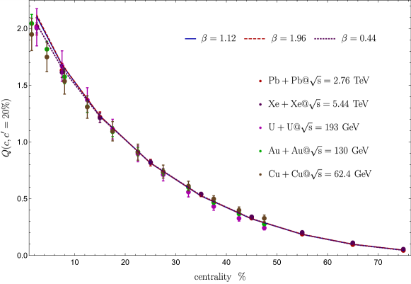
Figure 20: Universal centrality dependence of $Q(c,c^{\prime}{=}20))$, i.e. the number of produced charged particles normalised to $20$ centrality for each of the three models we consider. Experimental data shown for different collision systems: Xe+Xe [195], Pb+Pb [196], Au+Au [197],U+U [198], Cu+Cu [197]. The plot is taken from Ref. [176].

The impact of changing the initial state model can be assessed by fitting the parameter $\beta$ using the observed centrality dependence of the measured multiplicities. The formula Eq. (104) leads to a prediction in each centrality class. We then define the following ratios of multiplicities at different centralities

$$Q(c,c^{\prime})\equiv\frac{\langle\frac{dN}{dy}\rangle_{c^{\ }}}{\langle\frac{dN}{dy}\rangle_{c^{\prime}}}\leavevmode\nobreak\ ,$$ (115)

where the angle-brackets denote the mean value over events in the specified centrality class. These quantities are independent of the normalisation factors $C$ entering Eqns. (110), (113), (114); they are also independent of the factor $h(\beta)$, which depends on the shape of the presumptive attractor, not just its behaviour at early time. However, they retain dependence on the parameter $\beta$ itself, which is related to the attractor by Eq. (98). In this way, for any value of $\beta$, we obtain a set of numbers $Q(c,c^{\prime})$ which can be directly compared with published experimental results (see Fig. 20). The best fit for each of the three models is found to be

$$\beta^{\rm dilute-dense}=1.12,\quad\beta^{\rm IP}=1.96,\quad\beta^{\rm dense-dense}=0.44$$ (116)

with statistical errors not exceeding $0.02$. These values differ by a factor of almost $4.5$, which shows that if indeed an attractor determines early time behaviour, it is strongly connected to the initial state model. The implication here is that if we believe that QGP is free streaming at early times, then this places a constraint on the initial state model. Conversely, if we have reasons to favour a particular initial state model, then this may require accounting for corrections to free streaming at early times. These remarks should be relevant for Bayesian studies [199, 200, 201, 202], which scan over families of initial state models, but assume free-streaming prehydrodynamic evolution for all of them.

Beyond conformal Bjorken flow

The origin of attractor behaviour

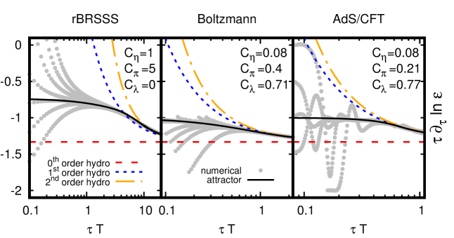
Figure 21: Hydrodynamic attractors in different theories. Plot form Ref. [17].

We have seen that in the case of Bjorken flow in conformal models of equilibration one can identify hydrodynamic attractors which extend into the far-from-equilibrium region. This is illustrated in Fig. 21 which presents the approximate attractors obtained for three different microscopic models. The appearance of attractors in these very different systems suggests that they are a generic feature of conformal theories undergoing Bjorken flow and are ultimately due to the specific kinematics of the earliest stages of ultrarelativistic heavy-ion collisions. These kinematic circumstances lead to simplifying symmetry assumptions such as boost invariance, conformal symmetry and the suppression of transverse dynamics. The resolution of the early thermalisation puzzle based on the notion of attractors relies on these assumptions remaining approximately valid for a sufficiently long time.

The physics of a heavy ion collision can be pictured as a competition between the longitudinal expansion resulting from the initial conditions and the interactions which drive the system toward equilibrium [21]. While the kinetic theory perspective makes this very explicit, the presence of an early-time, expansion dominated phase followed by a late-time regime interpreted in terms of nonhydrodynamic mode decay is also apparent in hydrodynamic models, as discussed in Section 4.5. Recently this point was amplified in Refs. [78, 117], where these two regimes were clearly distinguishable. As shown in Fig. 22, at late times generic solutions approach the attractor exponentially, with the rate set by the nonhydrodynamic mode frequency at vanishing wave vector. This interpretation is consistent with linear response, and has been verified in many examples. However, the behaviour at very early times, at least in the case of kinetic theory and hydrodynamic models, is not exponential, but follows a power law which is independent of the transport coefficients. The compelling explanation of this behaviour is that it is a consequence of the longitudinal expansion dominating over any transverse dynamics.

To assess the relevance of far-from-equilibrium hydrodynamic attractors to the physics of QGP at early times one needs to understand primarily the effects of conformal symmetry breaking and the onset of transverse dynamics. While a full exploration of these important issues remains a task for the future, a few notable results concerning these effects already exist in the literature [203, 204, 205, 206, 207, 121, 208, 120, 209] and some of them will be reviewed in this Section.

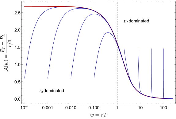
Figure 22: Log-linear plot showing different attraction mechanisms: expansion domination at early times, non-hydro mode decay at late times [78, 21].

Breaking conformal symmetry

The assumption of approximate conformal symmetry is valid in QCD at sufficiently high energies. Systematic theoretical studies and detailed comparison to available experimental data have provided constraints on the parameters appearing in the hydrodynamic description of QGP evolution, notably the bulk viscosity which is a sign of departures from conformality. The results of a multiparameter Bayesian fit of Ref. [199, 200] show that the effects of bulk viscosity are subdominant relative to shear, making the assumption of conformal invariance at early times look plausible. To quantify this effect in the pre-hydrodynamic stage the easiest thing to do is to assume that the free-streaming particles move with some effective velocity $v_{\rm fs}<1$, where $v_{\rm fs}=1$ is conformal. Experimental data suggest that $v_{\rm fs}\approx 0.82$ [199, 200], indicating some departure from conformality (see Fig. 23). Other recent studies which provide evidence for the effects of conformal symmetry breaking at the prehydrodynamic stage are reported in Refs. [210, 211].

Figure 23: Values of the shear (left) and the bulk (right) viscosity extracted from a Bayesian analysis of a $20$ parameter model of a HIC from Ref. [199, 200]. The horizontal black line on the left panel is the holographic prediction [58].

An important difference between conformal and non-conformal Bjorken flow is that in the latter case the energy momentum tensor Eq. (2) contains an additional degree of freedom, which (as discussed in Section 2.3) is eliminated by the tracelessness condition for conformal systems. Attractors in Bjorken flow without conformal symmetry were recently investigated in Refs. [204, 205, 206, 207, 120, 208]. Here we would like to mention one particular model of kinetic theory in the RTA, where conformal symmetry is broken due to quasiparticles of nonvanishing mass $m$ [212, 213]; this model also assumes a constant relaxation time $\tau_{R}$. Refs. [204, 205, 206] have identified a free-streaming far-from-equilibrium attractor in this model, however the hydrodynamic description employed there showed only a late-time attractor (in the near-equilibrium, hydrodynamic region). Here we will review the analysis of Ref. [121] which also studies this model, generalising the very suggestive approach to conformal Bjorken flow in RTA kinetic theory developed in Refs. [21, 214, 215, 216]. This analysis leads to a different hydrodynamic description of the system, which was found to reproduce the free-streaming attractor seen at the level of kinetic theory.

The basic idea of Refs. [21, 214, 215, 216] is to convert the Boltzmann kinetic equation to an infinite hierarchy of coupled ordinary differential equations describing a set of moments of the distribution function

$$\mathcal{L}_{n} \equiv \int_{\bf p}p_{0}\ P_{2n}(\cos\psi)\ f(\tau,p)\leavevmode\nobreak\ ,\qquad\forall n\geq 0$$ (117)

where $\cos\psi=p_{z}/p_{0}=v_{z}$ is constituent’s velocity along the $z-$direction, and $P_{2n}$ are Legendre polynomials of degree $2n$. These moments satisfy the following infinite hierarchy of equations which can be derived from the RTA Boltzmann equation Eq. (72)

$$\frac{\partial{\mathcal{L}_{0}}}{\partial{\tau}}= -\frac{1}{\tau}\left(a_{0}\mathcal{L}_{0}+c_{0}\mathcal{L}_{1}\right)\,,$$ (118a)

$$\frac{\partial{\mathcal{L}_{n}}}{\partial{\tau}}= -\frac{1}{\tau}\left(a_{n}\mathcal{L}_{n}+b_{n}\mathcal{L}_{n-1}+c_{n}\mathcal{L}_{n+1}\right)-\frac{\left(\mathcal{L}_{n}-\mathcal{L}_{n}^{\rm eq}\right)}{\tau_{R}}\,,\quad\forall n\geq 1\qquad$$ (118b)

where the coefficients $a_{n},b_{n},c_{n}$ are known explicitly [21, 121]

$$a_{n}=\frac{2(14n^{2}+7n-2)}{(4n-1)(4n+3)},\quad b_{n}=\frac{2n(2n-1)(3n+3)}{(4n-1)(4n+1)},\quad c_{n}=\frac{(1-2n)(2n+1)(2n+2)}{(4n+1)(4n+3)}\leavevmode\nobreak\ ,$$ (119)

and are determined entirely by the free-streaming part of the kinetic equation. The moments $\mathcal{L}_{n}^{\rm eq}$ are computed with the Boltzmann equilibrium distribution function $f_{\rm eq}(p_{0}/T)=\exp(-p_{0}/T)$, so for example $\mathcal{L}_{1}^{\rm eq}=\frac{1}{2}(\mathcal{E}-3P)$.

While in the conformal case the moments $\mathcal{L}_{n}$ are sufficient to provide a representation of the dynamics, in the nonconformal case the energy-momentum tensor is no longer traceless and this requires introducing a second set of moments. Indeed, from the general form of the energy-momentum tensor Eq. (2) for Bjorken flow it follows that

$$\mathcal{E}=\mathcal{L}_{0},\qquad\mathcal{P}_{L}=\frac{1}{3}\left(\mathcal{L}_{0}+2\mathcal{L}_{1}\right),\qquad\mathcal{P}_{T}=\frac{1}{3}\left(\mathcal{L}_{0}-\mathcal{L}_{1}-\frac{3}{2}T_{\mu}^{\mu}\right)\leavevmode\nobreak\ .$$ (120)

This motivates the introduction of another set of moments [121] in the following way:

$$\mathcal{M}_{n} \equiv m^{2}\int_{\bf p}\frac{1}{p_{0}}P_{2n}(\cos\psi)\ f(\tau,p),\qquad\forall n\geq 0\leavevmode\nobreak\ .$$ (121)

For example, the moment $\mathcal{M}_{0}$ is equal to the trace of the energy-momentum tensor:

$$\mathcal{M}_{0}=m^{2}\int_{\bf p}\frac{1}{p_{0}}f(\tau,p)=T^{\mu}_{\mu}=\mathcal{E}-\mathcal{P}_{L}-2\mathcal{P}_{T}\leavevmode\nobreak\ ,$$ (122)

and controls deviations from conformality. The RTA Boltzmann equation Eq. (72) can now be rewritten as an infinite hierarchy of equations with Eq. (118) supplemented by

$$\frac{\partial\mathcal{M}_{n}}{\partial\tau}=-\frac{1}{\tau}\left(a_{n}^{\prime}\mathcal{M}_{n}+b_{n}^{\prime}\mathcal{M}_{n-1}+c_{n}^{\prime}\mathcal{M}_{n+1}\right)-\frac{\mathcal{M}_{n}-\mathcal{M}^{\rm eq}_{n}}{\tau_{R}}\leavevmode\nobreak\ ,$$ (123)

where $\mathcal{M}^{\rm eq}_{n}$ are the equilibrium moments, and the coefficients read

$$a_{n}^{\prime}=\frac{2(6n^{2}+3n-1)}{(4n-1)(4n+3)},\quad b_{n}^{\prime}=\frac{4n^{2}(2n-1)}{(4n-1)(4n+1)},\quad c_{n}^{\prime}=-\frac{(2n+1)^{2}(2n+2)}{(4n+1)(4n+3)}\leavevmode\nobreak\ .$$ (124)

Note that the $\mathcal{M}_{n}$ moments are coupled to the $\mathcal{L}_{n}$ by the presence of the $\mathcal{M}^{\rm eq}_{n}$ terms, and decouple in the collisionless limit of $\tau_{R}\rightarrow\infty$. The equations Eq. (118) constitute a closed system which has to be solved first, determining the moments $\mathcal{L}_{n}$.

Using this infinite hierarchy of evolution equations one can identify an early-time far-from-equilibrium attractor which describes free-streaming. This is in line with results found in this model in Refs. [204, 205, 206]. Out of the three independent components of the energy-momentum tensor (see Eq. (3)), one has an attractor while the remaining two carry information about the initial state to the asymptotic late-time region. This can be contrasted with conformal systems, where the attractor appears in the pressure anisotropy, and information about the initial conditions is carried to asymptotically late times by the energy density alone.

In Ref. [121] the quantity which has an attractor is expressed as

$$g_{0}\equiv\frac{\tau}{\mathcal{L}_{0}}\frac{\partial\mathcal{L}_{0}}{\partial\tau}=-1-\frac{\mathcal{P}_{L}}{\mathcal{E}}.$$ (125)

In the conformal case this is trivially related to the pressure anisotropy, but in the absence of conformal symmetry it differs from it due to bulk pressure. For this reason the function $g_{0}$ does not satisfy a single ODE, as it would in a conformal model; instead, the pair of functions $g_{0},\mathcal{E}$ satisfy a coupled set of ODEs which determine their dynamics.

The attractor solution tends to $g_{0}=-1$ at early times, which corresponds to free streaming ($\mathcal{P}_{L}=0$). Its late-time behaviour is much harder to analyse than in the conformal case, since the equations of state are more involved. In particular, the velocity of sound tends to zero in this limit, which leads to rather nontrivial asymptotics [207, 217]. The hydrodynamic region is approached much more slowly and in way which depends of the mass. This behaviour is illustrated in Fig. 24.

Truncations of the hierarchy of evolution equations provide workable approximations which capture essential features of the full dynamics. The most straightforward truncation, which accounts for all three independent components of the energy-momentum tensor, consists of keeping $\mathcal{L}_{0}$, $\mathcal{L}_{1}$ and $\mathcal{M}_{0}$. The higher modes $\mathcal{L}_{2}$, and $\mathcal{M}_{1}$ coupled with the three lowest ones have to be modelled in some way, out of which the most simple, but not unreasonable, is to set $\mathcal{L}_{2}=\mathcal{M}_{1}=0$. This system of equations is hydrodynamic in spirit in the sense that it is a closed set of three ODEs. However, it is different from the hydrodynamic model used in Refs. [204, 205, 206]. The main virtue of this description is that it captures the early-time attractor identified in the underlying kinetic theory, as seen in Fig. 24. It should however be noted that it is obtained by truncating the boost-invariant moment hierarchy Eq. (118),  (123) and it is not entirely clear how it could be obtained from a set of covariant hydrodynamic equations such as variants of MIS theory [89, 47].

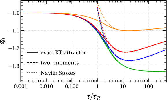
Figure 24: The attractor in the nonconformal kinetic model of Ref. [121], together attractors in effective hydrodynamic models (recall that $g_{0}$ is defined in Eq. (125)). The green, blue, red, and orange curves represent $m/T(\tau_{R})=0.001,0.5,1$, and $5$. “Two-moments” refers to the truncation with $\mathcal{L}_{2}=0$. This truncation clearly captures the early-time attraction, in contrast to the Navier-Stokes, which refers to the truncated gradient expansion. This plot is taken from Ref. [121].

Incorporating transverse dynamics

Since the longitudinal expansion is believed to be dominant at early times, the attractors seen in models of Bjorken flow may retain their relevance even in the presence of transverse dynamics. The persistence of early-time attractors in such circumstances was recently studied in Refs. [78, 218, 219] (see also Ref. [220]). The first of these papers considered transverse flow in the case of kinetic theory in the RTA. The authors have solved the boost-invariant Boltzmann equation numerically for a choice of realistic initial transverse profiles. It was found that as long as the transverse gradients remain negligible compared to the longitudinal ones at initialisation time, arbitrary initial conditions in 3+1D evolve towards the 1+1D attractor. The late-time evolution does however depend on the transverse profile of energy and transverse momentum, reflecting the fact that the space of solutions of boost-invariant perfect fluid hydrodynamics has a higher dimensionality than what is seen in the case of Bjorken flow. These results suggests a degree of robustness of early time attractors in the presence of transverse dynamics.

Other work on attractors with transverse dynamics includes studies of Gubser flow [221, 111, 115, 222] (this activity was recently reviewed by Soloviev [24]). The applicability of hydrodynamics, including the effects of the build-up of transverse dynamics at early times was also the subject of recent Refs. [182, 181, 183].

Outlook

In this review we have attempted to present the main ideas behind the hypothesis that the applicability of fluid dynamics to early phases of QGP dynamics can be explained by a far-from-equilibrium hydrodynamic attractor. We have emphasised the role of the kinematic setting specific to heavy-ion collisions, which makes it plausible that such an attractor occurs also in QCD. At the conceptual level this picture is rather compelling. However, Bjorken flow is a very restrictive setting, and despite some existing applications using the attractor in practical calculations of phenomenologically interesting observables requires developing effective methods of working with models with a large number of degrees of freedom. Progress is likely to come gradually, by learning how to deal with models of increasing complexity, extending the studies reviewed in Sections 7 and 9.

The idea of hydrodynamic attractors has been closely connected with the divergence of the hydrodynamic gradient expansion. In this review we have not discussed this connection beyond its utilitarian aspects, but on a conceptual level there have been some important developments in recent times. This includes a proof of the generic divergence of the gradient expansion at the linearised level without any symmetry assumptions, and its connection with the properties of dispersion relations [48, 97]. At the nonlinear level, some of the results for Bjorken flow have been generalised to a much wider class of flows, called longitudinal flows. In particular, the gradient expansion has been shown to diverge for this class of solutions [98]. It was also found that the large order behaviour of the gradient series can be expressed in terms of new degrees of freedom, the singulant fields, which track transient effects [62]. The relevance of these advances to the study of attractors remains an interesting challenge for the future.

A number of issues were not addressed in this review. One is the presence of other degrees of freedom, such as those connected with chiral symmetry breaking, and their possible effect on the attractor dynamics of QGP [223, 224] (see also Ref. [225]). Another such issue is the role of fluctuations, which has been mostly neglected in the attractor literature, with the notable exception of Refs. [226, 227].

It would also be very interesting to understand the role of quantum effects in the early-time dynamics. Of course the hydrodynamic picture implicitly contains them, but in a rather opaque way. On the other hand, the kinetic theory description arises from quantum field theory through a series of approximations [228, 229] and it should be possible to study the origin and robustness of the kinetic theory attractor in a framework which allows for a systematic incorporation of quantum corrections. This is connected with other approaches to early-time dynamics, including those involving ideas such as the Color Glass Condensate or non-thermal attractors [230, 231, 232, 233, 234, 23]. It is not yet fully understood how they are related to the ideas reviewed here, and clarifying this appears to be a very promising avenue for future research.

Finally, there is the more general question about far-from-equilibrium attractors in nonequilibrium systems. In the context of heavy-ion collisions the specific kinematic circumstances have lead us to consider boost-invariant expansion where far-from-equilibrium hydrodynamic behaviour was first noted, but there could be other situations where analogous phenomena might appear [235], perhaps even in the non-relativistic domain [236]. Another context where far from equilibrium hydrodynamic attractors can occur is the dynamics of systems in nontrivial spacetime backgrounds (see e.g. Ref. [237]).

Acknowledgements We would like to thank many of our colleagues with whom we have had countless discussions about attractors over the years. This includes especially Wojciech Florkowski, Michał Heller and Viktor Svensson. JJ is supported by the National Science Centre, Poland, under grant 2018/29/B/ST2/02457. MS is supported by the National Science Centre, Poland, under grants 2018/29/B/ST2/02457 and 2021/41/B/ST2/02909. For the purpose of Open Access, the author has applied a CC-BY public copyright licence to any Author Accepted Manuscript (AAM) version arising from this submission.

References

- [1] P. F. Kolb, U. W. Heinz, Hydrodynamic description of ultrarelativistic heavy ion collisions, (2003) 634arXiv:nucl-th/0305084.
- [2] U. Heinz, R. Snellings, Collective flow and viscosity in relativistic heavy-ion collisions, Ann. Rev. Nucl. Part. Sci. 63 (2013) 123–151. arXiv:1301.2826, doi:10.1146/annurev-nucl-102212-170540.
- [3] W. Busza, K. Rajagopal, W. van der Schee, Heavy Ion Collisions: The Big Picture, and the Big Questions, Ann. Rev. Nucl. Part. Sci. 68 (2018) 339–376. arXiv:1802.04801, doi:10.1146/annurev-nucl-101917-020852.
- [4] B. Schenke, The smallest fluid on Earth, Rept. Prog. Phys. 84 (8) (2021) 082301. arXiv:2102.11189, doi:10.1088/1361-6633/ac14c9.
- [5] A. Lovato, et al., Long Range Plan: Dense matter theory for heavy-ion collisions and neutron stars (11 2022). arXiv:2211.02224.
- [6] A. Sorensen, et al., Dense Nuclear Matter Equation of State from Heavy-Ion Collisions (1 2023). arXiv:2301.13253.
- [7] P. Achenbach, et al., The Present and Future of QCD (3 2023). arXiv:2303.02579.
- [8] I. Muller, Zum Paradoxon der Warmeleitungstheorie, Z. Phys. 198 (1967) 329–344. doi:10.1007/BF01326412.
- [9] W. Israel, Nonstationary irreversible thermodynamics: A Causal relativistic theory, Annals Phys. 100 (1976) 310–331. doi:10.1016/0003-4916(76)90064-6.
- [10] W. Israel, J. M. Stewart, Transient relativistic thermodynamics and kinetic theory, Annals Phys. 118 (1979) 341–372. doi:10.1016/0003-4916(79)90130-1.
- [11] U. W. Heinz, P. F. Kolb, Two RHIC puzzles: Early thermalization and the HBT problem, in: 18th Winter Workshop on Nuclear Dynamics, 2002, pp. 1–12. arXiv:hep-ph/0204061.
- [12] P. Romatschke, U. Romatschke, Viscosity Information from Relativistic Nuclear Collisions: How Perfect is the Fluid Observed at RHIC?, Phys. Rev. Lett. 99 (2007) 172301. arXiv:0706.1522, doi:10.1103/PhysRevLett.99.172301.
- [13] D. Teaney, The Effects of viscosity on spectra, elliptic flow, and HBT radii, Phys. Rev. C 68 (2003) 034913. arXiv:nucl-th/0301099, doi:10.1103/PhysRevC.68.034913.
- [14] M. P. Heller, M. Spaliński, Hydrodynamics Beyond the Gradient Expansion: Resurgence and Resummation, Phys. Rev. Lett. 115 (7) (2015) 072501. arXiv:1503.07514, doi:10.1103/PhysRevLett.115.072501.
- [15] K. Yagi, T. Hatsuda, Y. Miake, Quark-gluon plasma: From big bang to little bang, Vol. 23, Cambridge University Press, 2005.
- [16] J. D. Bjorken, Highly Relativistic Nucleus-Nucleus Collisions: The Central Rapidity Region, Phys. Rev. D 27 (1983) 140–151. doi:10.1103/PhysRevD.27.140.
- [17] P. Romatschke, Relativistic Fluid Dynamics Far From Local Equilibrium, Phys. Rev. Lett. 120 (1) (2018) 012301. arXiv:1704.08699, doi:10.1103/PhysRevLett.120.012301.
- [18] M. Strickland, The non-equilibrium attractor for kinetic theory in relaxation time approximation, JHEP 12 (2018) 128. arXiv:1809.01200, doi:10.1007/JHEP12(2018)128.
- [19] D. Almaalol, A. Kurkela, M. Strickland, Nonequilibrium Attractor in High-Temperature QCD Plasmas, Phys. Rev. Lett. 125 (12) (2020) 122302. arXiv:2004.05195, doi:10.1103/PhysRevLett.125.122302.
- [20] J. Noronha, M. Spaliński, E. Speranza, Transient Relativistic Fluid Dynamics in a General Hydrodynamic Frame, Phys. Rev. Lett. 128 (25) (2022) 252302. arXiv:2105.01034, doi:10.1103/PhysRevLett.128.252302.
- [21] J.-P. Blaizot, L. Yan, Fluid dynamics of out of equilibrium boost invariant plasmas, Phys. Lett. B 780 (2018) 283–286. arXiv:1712.03856, doi:10.1016/j.physletb.2018.02.058.
- [22] W. Florkowski, M. P. Heller, M. Spalinski, New theories of relativistic hydrodynamics in the LHC era, Rept. Prog. Phys. 81 (4) (2018) 046001. arXiv:1707.02282, doi:10.1088/1361-6633/aaa091.
- [23] J. Berges, M. P. Heller, A. Mazeliauskas, R. Venugopalan, QCD thermalization: Ab initio approaches and interdisciplinary connections, Rev. Mod. Phys. 93 (3) (2021) 035003. arXiv:2005.12299, doi:10.1103/RevModPhys.93.035003.
- [24] A. Soloviev, Hydrodynamic attractors in heavy ion collisions: a review, Eur. Phys. J. C 82 (4) (2022) 319. arXiv:2109.15081, doi:10.1140/epjc/s10052-022-10282-4.
- [25] M. Strickland, Anisotropic Hydrodynamics: Three lectures, Acta Phys. Polon. B 45 (12) (2014) 2355–2394. arXiv:1410.5786, doi:10.5506/APhysPolB.45.2355.
- [26] K. Gottfried, Space-Time Structure of Hadronic Collisions and Nuclear Multiple Production, Phys. Rev. Lett. 32 (1974) 957–961. doi:10.1103/PhysRevLett.32.957.
- [27] F. E. Low, K. Gottfried, Classical Space-Time Concepts in High-Energy Collisions, Phys. Rev. D 17 (1978) 2487. doi:10.1103/PhysRevD.17.2487.
- [28] R. Anishetty, P. Koehler, L. D. McLerran, Central Collisions Between Heavy Nuclei at Extremely High-Energies: The Fragmentation Region, Phys. Rev. D 22 (1980) 2793. doi:10.1103/PhysRevD.22.2793.
- [29] B. B. Back, et al., The Significance of the fragmentation region in ultrarelativistic heavy ion collisions, Phys. Rev. Lett. 91 (2003) 052303. arXiv:nucl-ex/0210015, doi:10.1103/PhysRevLett.91.052303.
- [30] M. D. Baker, et al., Global observations from PHOBOS, Nucl. Phys. A 715 (2003) 65–74. arXiv:nucl-ex/0212009, doi:10.1016/S0375-9474(02)01414-8.
- [31] J. S. Moreland, J. E. Bernhard, S. A. Bass, Bayesian calibration of a hybrid nuclear collision model using p-Pb and Pb-Pb data at energies available at the CERN Large Hadron Collider, Phys. Rev. C 101 (2) (2020) 024911. arXiv:1808.02106, doi:10.1103/PhysRevC.101.024911.
- [32] J. P. Blaizot, A. H. Mueller, The Early Stage of Ultrarelativistic Heavy Ion Collisions, Nucl. Phys. B 289 (1987) 847–860. doi:10.1016/0550-3213(87)90408-1.
- [33] R. Baier, A. H. Mueller, D. Schiff, D. T. Son, ’Bottom up’ thermalization in heavy ion collisions, Phys. Lett. B 502 (2001) 51–58. arXiv:hep-ph/0009237, doi:10.1016/S0370-2693(01)00191-5.
- [34] S. Schlichting, D. Teaney, The First fm/c of Heavy-Ion Collisions, Ann. Rev. Nucl. Part. Sci. 69 (2019) 447–476. arXiv:1908.02113, doi:10.1146/annurev-nucl-101918-023825.
- [35] P. Romatschke, New Developments in Relativistic Viscous Hydrodynamics, Int. J. Mod. Phys. E 19 (2010) 1–53. arXiv:0902.3663, doi:10.1142/S0218301310014613.
- [36] P. Romatschke, U. Romatschke, Relativistic Fluid Dynamics In and Out of Equilibrium, Cambridge Monographs on Mathematical Physics, Cambridge University Press, 2019. arXiv:1712.05815, doi:10.1017/9781108651998.
- [37] R. Loganayagam, Entropy Current in Conformal Hydrodynamics, JHEP 05 (2008) 087. arXiv:0801.3701, doi:10.1088/1126-6708/2008/05/087.
- [38] W. A. Hiscock, L. Lindblom, Stability and causality in dissipative relativistic fluids, Annals Phys. 151 (1983) 466–496. doi:10.1016/0003-4916(83)90288-9.
- [39] W. A. Hiscock, L. Lindblom, Generic instabilities in first-order dissipative relativistic fluid theories, Phys. Rev. D 31 (1985) 725–733. doi:10.1103/PhysRevD.31.725.
- [40] L. Gavassino, Can We Make Sense of Dissipation without Causality?, Phys. Rev. X 12 (4) (2022) 041001. arXiv:2111.05254, doi:10.1103/PhysRevX.12.041001.
- [41] F. S. Bemfica, M. M. Disconzi, J. Noronha, Causality and existence of solutions of relativistic viscous fluid dynamics with gravity, Phys. Rev. D 98 (10) (2018) 104064. arXiv:1708.06255, doi:10.1103/PhysRevD.98.104064.
- [42] F. S. Bemfica, M. M. Disconzi, J. Noronha, Causality of the Einstein-Israel-Stewart Theory with Bulk Viscosity, Phys. Rev. Lett. 122 (22) (2019) 221602. arXiv:1901.06701, doi:10.1103/PhysRevLett.122.221602.
- [43] F. S. Bemfica, M. M. Disconzi, V. Hoang, J. Noronha, M. Radosz, Nonlinear Constraints on Relativistic Fluids Far from Equilibrium, Phys. Rev. Lett. 126 (22) (2021) 222301. arXiv:2005.11632, doi:10.1103/PhysRevLett.126.222301.
- [44] F. S. Bemfica, M. M. Disconzi, J. Noronha, Nonlinear Causality of General First-Order Relativistic Viscous Hydrodynamics, Phys. Rev. D 100 (10) (2019) 104020. arXiv:1907.12695, doi:10.1103/PhysRevD.100.104020.
- [45] F. S. Bemfica, M. M. Disconzi, J. Noronha, First-Order General-Relativistic Viscous Fluid Dynamics, Phys. Rev. X 12 (2) (2022) 021044. arXiv:2009.11388, doi:10.1103/PhysRevX.12.021044.
- [46] S. Bhattacharyya, V. E. Hubeny, S. Minwalla, M. Rangamani, Nonlinear Fluid Dynamics from Gravity, JHEP 02 (2008) 045. arXiv:0712.2456, doi:10.1088/1126-6708/2008/02/045.
- [47] R. Baier, P. Romatschke, D. T. Son, A. O. Starinets, M. A. Stephanov, Relativistic viscous hydrodynamics, conformal invariance, and holography, JHEP 04 (2008) 100. arXiv:0712.2451, doi:10.1088/1126-6708/2008/04/100.
- [48] B. Withers, Short-lived modes from hydrodynamic dispersion relations, JHEP 06 (2018) 059. arXiv:1803.08058, doi:10.1007/JHEP06(2018)059.
- [49] S. Grozdanov, P. K. Kovtun, A. O. Starinets, P. Tadić, The complex life of hydrodynamic modes, JHEP 11 (2019) 097. arXiv:1904.12862, doi:10.1007/JHEP11(2019)097.
- [50] M. P. Heller, A. Serantes, M. Spaliński, V. Svensson, B. Withers, Convergence of hydrodynamic modes: insights from kinetic theory and holography, SciPost Phys. 10 (2021) 123. arXiv:2012.15393, doi:10.21468/SciPostPhys.10.6.123.
- [51] M. P. Heller, A. Serantes, M. Spaliński, V. Svensson, B. Withers, Transseries for causal diffusive systems, JHEP 04 (2021) 192. arXiv:2011.13864, doi:10.1007/JHEP04(2021)192.
- [52] M. Spaliński, Small systems and regulator dependence in relativistic hydrodynamics, Phys. Rev. D 94 (8) (2016) 085002. arXiv:1607.06381, doi:10.1103/PhysRevD.94.085002.
- [53] P. Kovtun, First-order relativistic hydrodynamics is stable, JHEP 10 (2019) 034. arXiv:1907.08191, doi:10.1007/JHEP10(2019)034.
- [54] M. P. Heller, R. A. Janik, M. Spaliński, P. Witaszczyk, Coupling hydrodynamics to nonequilibrium degrees of freedom in strongly interacting quark-gluon plasma, Phys. Rev. Lett. 113 (26) (2014) 261601. arXiv:1409.5087, doi:10.1103/PhysRevLett.113.261601.
- [55] M. P. Heller, A. Serantes, M. Spaliński, B. Withers, Rigorous bounds on transport from causality (12 2022). arXiv:2212.07434.
- [56] L. Gavassino, Bounds on transport from hydrodynamic stability (1 2023). arXiv:2301.06651.
- [57] P. Romatschke, Retarded correlators in kinetic theory: branch cuts, poles and hydrodynamic onset transitions, Eur. Phys. J. C 76 (6) (2016) 352. arXiv:1512.02641, doi:10.1140/epjc/s10052-016-4169-7.
- [58] P. Kovtun, D. T. Son, A. O. Starinets, Viscosity in strongly interacting quantum field theories from black hole physics, Phys. Rev. Lett. 94 (2005) 111601. arXiv:hep-th/0405231, doi:10.1103/PhysRevLett.94.111601.
- [59] H. Bantilan, Y. Bea, P. Figueras, Evolutions in first-order viscous hydrodynamics, JHEP 08 (2022) 298. arXiv:2201.13359, doi:10.1007/JHEP08(2022)298.
- [60] I. Aniceto, M. Spaliński, Resurgence in Extended Hydrodynamics, Phys. Rev. D 93 (8) (2016) 085008. arXiv:1511.06358, doi:10.1103/PhysRevD.93.085008.
- [61] L. Gavassino, M. Antonelli, B. Haskell, Symmetric-hyperbolic quasihydrodynamics, Phys. Rev. D 106 (5) (2022) 056010. arXiv:2207.14778, doi:10.1103/PhysRevD.106.056010.
- [62] M. P. Heller, A. Serantes, M. Spaliński, V. Svensson, B. Withers, Relativistic Hydrodynamics: A Singulant Perspective, Phys. Rev. X 12 (4) (2022) 041010. arXiv:2112.12794, doi:10.1103/PhysRevX.12.041010.
- [63] M. Stephanov, Y. Yin, Hydrodynamics with parametric slowing down and fluctuations near the critical point, Phys. Rev. D 98 (3) (2018) 036006. arXiv:1712.10305, doi:10.1103/PhysRevD.98.036006.
- [64] N. Abbasi, M. Kaminski, Constraints on quasinormal modes and bounds for critical points from pole-skipping, JHEP 03 (2021) 265. arXiv:2012.15820, doi:10.1007/JHEP03(2021)265.
- [65] W. Ke, Y. Yin, Does quark-gluon plasma feature an extended hydrodynamic regime? (8 2022). arXiv:2208.01046.
- [66] R. E. Hoult, P. Kovtun, Stable and causal relativistic Navier-Stokes equations, JHEP 06 (2020) 067. arXiv:2004.04102, doi:10.1007/JHEP06(2020)067.
- [67] A. Pandya, F. Pretorius, Numerical exploration of first-order relativistic hydrodynamics, Phys. Rev. D 104 (2) (2021) 023015. arXiv:2104.00804, doi:10.1103/PhysRevD.104.023015.
- [68] A. Pandya, E. R. Most, F. Pretorius, Conservative finite volume scheme for first-order viscous relativistic hydrodynamics, Phys. Rev. D 105 (12) (2022) 123001. arXiv:2201.12317, doi:10.1103/PhysRevD.105.123001.
- [69] A. Pandya, E. R. Most, F. Pretorius, Causal, stable first-order viscous relativistic hydrodynamics with ideal gas microphysics (9 2022). arXiv:2209.09265.
- [70] L. Gavassino, M. M. Disconzi, J. Noronha, Universality Classes of Relativistic Fluid Dynamics I: Foundations (2 2023). arXiv:2302.03478.
- [71] L. Gavassino, M. M. Disconzi, J. Noronha, Universality Classes of Relativistic Fluid Dynamics II: Applications (2 2023). arXiv:2302.05332.
- [72] L. Gavassino, M. Antonelli, B. Haskell, When the entropy has no maximum: a new perspective on the instability of the first-order theories of dissipation, Phys. Rev. D 102 (4) (2020) 043018. arXiv:2006.09843, doi:10.1103/PhysRevD.102.043018.
- [73] L. Gavassino, Applying the Gibbs stability criterion to relativistic hydrodynamics, Class. Quant. Grav. 38 (21) (2021) 21LT02. arXiv:2104.09142, doi:10.1088/1361-6382/ac2b0e.
- [74] V. Mukhanov, Physical Foundations of Cosmology, Cambridge University Press, Cambridge, 2005. doi:10.1017/CBO9780511790553.
- [75] C. Cartwright, M. Kaminski, M. Knipfer, Hydrodynamic attractors for the speed of sound in holographic Bjorken flow (7 2022). arXiv:2207.02875.
- [76] M. Strickland, J. Noronha, G. Denicol, Anisotropic nonequilibrium hydrodynamic attractor, Phys. Rev. D 97 (3) (2018) 036020. arXiv:1709.06644, doi:10.1103/PhysRevD.97.036020.
- [77] M. Alqahtani, N. Demir, M. Strickland, Nonextensive hydrodynamics of boost-invariant plasmas (3 2022). arXiv:2203.14968.
- [78] A. Kurkela, W. van der Schee, U. A. Wiedemann, B. Wu, Early- and Late-Time Behavior of Attractors in Heavy-Ion Collisions, Phys. Rev. Lett. 124 (10) (2020) 102301. arXiv:1907.08101, doi:10.1103/PhysRevLett.124.102301.
- [79] I. Aniceto, D. Hasenbichler, A. O. Daalhuis, The late to early time behaviour of an expanding plasma: hydrodynamisation from exponential asymptotics (7 2022). arXiv:2207.02868.
- [80] M. P. Heller, A. Kurkela, M. Spaliński, V. Svensson, Hydrodynamization in kinetic theory: Transient modes and the gradient expansion, Phys. Rev. D 97 (9) (2018) 091503. arXiv:1609.04803, doi:10.1103/PhysRevD.97.091503.
- [81] G. Basar, G. V. Dunne, Hydrodynamics, resurgence, and transasymptotics, Phys. Rev. D 92 (12) (2015) 125011. arXiv:1509.05046, doi:10.1103/PhysRevD.92.125011.
- [82] R. A. Janik, R. B. Peschanski, Gauge/gravity duality and thermalization of a boost-invariant perfect fluid, Phys. Rev. D 74 (2006) 046007. arXiv:hep-th/0606149, doi:10.1103/PhysRevD.74.046007.
- [83] M. Spaliński, Universal behaviour, transients and attractors in supersymmetric Yang–Mills plasma, Phys. Lett. B 784 (2018) 21–25. arXiv:1805.11689, doi:10.1016/j.physletb.2018.07.003.
- [84] G. S. Denicol, J. Noronha, Exact hydrodynamic attractor of an ultrarelativistic gas of hard spheres, Phys. Rev. Lett. 124 (15) (2020) 152301. arXiv:1908.09957, doi:10.1103/PhysRevLett.124.152301.
- [85] M. Strickland, U. Tantary, Exact solution for the non-equilibrium attractor in number-conserving relaxation time approximation, JHEP 10 (2019) 069. arXiv:1903.03145, doi:10.1007/JHEP10(2019)069.
- [86] A. R. Liddle, P. Parsons, J. D. Barrow, Formalizing the slow roll approximation in inflation, Phys. Rev. D 50 (1994) 7222–7232. arXiv:astro-ph/9408015, doi:10.1103/PhysRevD.50.7222.
- [87] M. Spalinski, On the Slow Roll Expansion for Brane Inflation, JCAP 04 (2007) 018. arXiv:hep-th/0702118, doi:10.1088/1475-7516/2007/04/018.
- [88] S. Jaiswal, C. Chattopadhyay, A. Jaiswal, S. Pal, U. Heinz, Exact solutions and attractors of higher-order viscous fluid dynamics for Bjorken flow, Phys. Rev. C 100 (3) (2019) 034901. arXiv:1907.07965, doi:10.1103/PhysRevC.100.034901.
- [89] G. S. Denicol, H. Niemi, E. Molnar, D. H. Rischke, Derivation of transient relativistic fluid dynamics from the Boltzmann equation, Phys. Rev. D 85 (2012) 114047, [Erratum: Phys.Rev.D 91, 039902 (2015)]. arXiv:1202.4551, doi:10.1103/PhysRevD.85.114047.
- [90] A. Jaiswal, Relativistic third-order dissipative fluid dynamics from kinetic theory, Phys. Rev. C 88 (2013) 021903. arXiv:1305.3480, doi:10.1103/PhysRevC.88.021903.
- [91] L. J. Naik, S. Jaiswal, K. Sreelakshmi, A. Jaiswal, V. Sreekanth, Hydrodynamical attractor and thermal particle production in heavy-ion collision, (7 2021). arXiv:2107.08791.
- [92] G. S. Denicol, J. Noronha, Analytical attractor and the divergence of the slow-roll expansion in relativistic hydrodynamics, Phys. Rev. D 97 (5) (2018) 056021. arXiv:1711.01657, doi:10.1103/PhysRevD.97.056021.
- [93] J.-P. Blaizot, L. Yan, Analytical attractor for Bjorken flows, Phys. Lett. B 820 (2021) 136478. arXiv:2006.08815, doi:10.1016/j.physletb.2021.136478.
- [94] M. P. Heller, R. A. Janik, P. Witaszczyk, Hydrodynamic Gradient Expansion in Gauge Theory Plasmas, Phys. Rev. Lett. 110 (21) (2013) 211602. arXiv:1302.0697, doi:10.1103/PhysRevLett.110.211602.
- [95] G. S. Denicol, J. Noronha, Divergence of the Chapman-Enskog expansion in relativistic kinetic theory (8 2016). arXiv:1608.07869.
- [96] W. Florkowski, R. Ryblewski, M. Spaliński, Gradient expansion for anisotropic hydrodynamics, Phys. Rev. D 94 (11) (2016) 114025. arXiv:1608.07558, doi:10.1103/PhysRevD.94.114025.
- [97] M. P. Heller, A. Serantes, M. Spaliński, V. Svensson, B. Withers, Hydrodynamic gradient expansion in linear response theory, Phys. Rev. D 104 (6) (2021) 066002. arXiv:2007.05524, doi:10.1103/PhysRevD.104.066002.
- [98] M. P. Heller, A. Serantes, M. Spaliński, V. Svensson, B. Withers, Hydrodynamic Gradient Expansion Diverges beyond Bjorken Flow, Phys. Rev. Lett. 128 (12) (2022) 122302. arXiv:2110.07621, doi:10.1103/PhysRevLett.128.122302.
- [99] C. M. Bender, S. A. Orszag, Advanced Mathematical Methods for Scientists and Engineers, McGraw-Hill, 1978.
- [100] R. Dingle, Asymptotic expansions: their derivation and interpretation, Vol. 521, Academic Press London, 1973.
-
[101]
M. Berry, Asymptotics,
Superasymptotics, Hyperasymptotics…, Springer US, Boston, MA, 1991, pp.
1–14.
doi:10.1007/978-1-4757-0435-8_1.
URL https://doi.org/10.1007/978-1-4757-0435-8_1 - [102] C. M. Bender, C. Heissenberg, Convergent and Divergent Series in Physics, in: 22nd Saalburg Summer School on Foundations and New Methods in Theoretical Physics, 2017. arXiv:1703.05164.
- [103] O. Costin, G. V. Dunne, Physical Resurgent Extrapolation, Phys. Lett. B 808 (2020) 135627. arXiv:2003.07451, doi:10.1016/j.physletb.2020.135627.
- [104] O. Costin, G. V. Dunne, Uniformization and Constructive Analytic Continuation of Taylor Series, Commun. Math. Phys. 392 (2022) 863–906. arXiv:2009.01962, doi:10.1007/s00220-022-04361-6.
- [105] O. Costin, G. V. Dunne, Conformal and uniformizing maps in Borel analysis, Eur. Phys. J. ST 230 (12-13) (2021) 2679–2690. arXiv:2108.01145, doi:10.1140/epjs/s11734-021-00267-x.
- [106] O. Costin, G. V. Dunne, M. Meynig, Noise Effects on Pade Approximants and Conformal Maps (8 2022). arXiv:2208.02410.
- [107] I. Aniceto, G. Basar, R. Schiappa, A Primer on Resurgent Transseries and Their Asymptotics, Phys. Rept. 809 (2019) 1–135. arXiv:1802.10441, doi:10.1016/j.physrep.2019.02.003.
- [108] C. Mitschi, D. Sauzin, Divergent Series, Summability and Resurgence I, Vol. 2153, Springer, 2016. doi:10.1007/978-3-319-28736-2.
- [109] M. Shokri, F. Taghinavaz, Conformal Bjorken flow in the general frame and its attractor: Similarities and discrepancies with the Müller-Israel-Stewart formalism, Phys. Rev. D 102 (3) (2020) 036022. arXiv:2002.04719, doi:10.1103/PhysRevD.102.036022.
- [110] G. S. Rocha, G. S. Denicol, J. Noronha, Perturbative approaches in relativistic kinetic theory and the emergence of first-order hydrodynamics, Phys. Rev. D 106 (3) (2022) 036010. arXiv:2205.00078, doi:10.1103/PhysRevD.106.036010.
- [111] A. Behtash, C. N. Cruz-Camacho, M. Martinez, Far-from-equilibrium attractors and nonlinear dynamical systems approach to the Gubser flow, Phys. Rev. D 97 (4) (2018) 044041. arXiv:1711.01745, doi:10.1103/PhysRevD.97.044041.
- [112] M. P. Heller, V. Svensson, How does relativistic kinetic theory remember about initial conditions?, Phys. Rev. D 98 (5) (2018) 054016. arXiv:1802.08225, doi:10.1103/PhysRevD.98.054016.
- [113] A. Behtash, C. N. Cruz-Camacho, S. Kamata, M. Martinez, Non-perturbative rheological behavior of a far-from-equilibrium expanding plasma, Phys. Lett. B 797 (2019) 134914. arXiv:1805.07881, doi:10.1016/j.physletb.2019.134914.
- [114] A. Behtash, S. Kamata, M. Martinez, H. Shi, Dynamical systems and nonlinear transient rheology of the far-from-equilibrium Bjorken flow, Phys. Rev. D 99 (11) (2019) 116012. arXiv:1901.08632, doi:10.1103/PhysRevD.99.116012.
- [115] A. Behtash, S. Kamata, M. Martinez, H. Shi, Global flow structure and exact formal transseries of the Gubser flow in kinetic theory, JHEP 07 (2020) 226. arXiv:1911.06406, doi:10.1007/JHEP07(2020)226.
- [116] C. Chattopadhyay, U. W. Heinz, Hydrodynamics from free-streaming to thermalization and back again, Phys. Lett. B 801 (2020) 135158. arXiv:1911.07765, doi:10.1016/j.physletb.2019.135158.
- [117] M. P. Heller, R. Jefferson, M. Spaliński, V. Svensson, Hydrodynamic Attractors in Phase Space, Phys. Rev. Lett. 125 (13) (2020) 132301. arXiv:2003.07368, doi:10.1103/PhysRevLett.125.132301.
- [118] M. McNelis, U. Heinz, Hydrodynamic generators in relativistic kinetic theory, Phys. Rev. C 101 (5) (2020) 054901. arXiv:2001.09125, doi:10.1103/PhysRevC.101.054901.
- [119] S. Kamata, M. Martinez, P. Plaschke, S. Ochsenfeld, S. Schlichting, Hydrodynamization and nonequilibrium Green’s functions in kinetic theory, Phys. Rev. D 102 (5) (2020) 056003. arXiv:2004.06751, doi:10.1103/PhysRevD.102.056003.
- [120] H. Alalawi, M. Strickland, Far-from-equilibrium attractors for massive kinetic theory in the relaxation time approximation, JHEP 12 (2022) 143. arXiv:2210.00658, doi:10.1007/JHEP12(2022)143.
- [121] S. Jaiswal, J.-P. Blaizot, R. S. Bhalerao, Z. Chen, A. Jaiswal, L. Yan, From moments of the distribution function to hydrodynamics the non-conformal case, (8 2022). arXiv:2208.02750.
- [122] J. L. Anderson, H. R. Witting, A relativistic relaxation-time model for the Boltzmann equation, Physica 74 (1974) 466.
- [123] P. B. Arnold, G. D. Moore, L. G. Yaffe, Effective kinetic theory for high temperature gauge theories, JHEP 01 (2003) 030. arXiv:hep-ph/0209353, doi:10.1088/1126-6708/2003/01/030.
- [124] G. S. Rocha, G. S. Denicol, J. Noronha, Novel Relaxation Time Approximation to the Relativistic Boltzmann Equation, Phys. Rev. Lett. 127 (4) (2021) 042301. arXiv:2103.07489, doi:10.1103/PhysRevLett.127.042301.
- [125] G. S. Rocha, G. S. Denicol, Transient fluid dynamics with general matching conditions: A first study from the method of moments, Phys. Rev. D 104 (9) (2021) 096016. arXiv:2108.02187, doi:10.1103/PhysRevD.104.096016.
- [126] D. Dash, S. Bhadury, S. Jaiswal, A. Jaiswal, Extended relaxation time approximation and relativistic dissipative hydrodynamics, Phys. Lett. B 831 (2022) 137202. arXiv:2112.14581, doi:10.1016/j.physletb.2022.137202.
- [127] G. S. Denicol, J. Noronha, Exact results for the Boltzmann collision operator in theory (9 2022). arXiv:2209.10370.
- [128] G. Baym, Thermal Equilibration in ultrarelativistic heavy ion collisions, Phys. Lett. B 138 (1984) 18–22. doi:10.1016/0370-2693(84)91863-X.
- [129] W. Florkowski, R. Ryblewski, M. Strickland, Anisotropic Hydrodynamics for Rapidly Expanding Systems, Nucl. Phys. A 916 (2013) 249–259. arXiv:1304.0665, doi:10.1016/j.nuclphysa.2013.08.004.
- [130] A. Bialas, W. Czyz, Boost Invariant Boltzmann-vlasov Equations for Relativistic Quark - Anti-quark Plasma, Phys. Rev. D 30 (1984) 2371. doi:10.1103/PhysRevD.30.2371.
- [131] A. Bialas, W. Czyz, A. Dyrek, W. Florkowski, Oscillations of Quark - Gluon Plasma Generated in Strong Color Fields, Nucl. Phys. B 296 (1988) 611–624. doi:10.1016/0550-3213(88)90035-1.
- [132] S. R. De Groot, Relativistic Kinetic Theory. Principles and Applications, 1980.
- [133] A. Jaiswal, Relativistic dissipative hydrodynamics from kinetic theory with relaxation time approximation, Phys. Rev. C 87 (5) (2013) 051901. arXiv:1302.6311, doi:10.1103/PhysRevC.87.051901.
- [134] P. Romatschke, M. Strickland, Collective modes of an anisotropic quark gluon plasma, Phys. Rev. D 68 (2003) 036004. arXiv:hep-ph/0304092, doi:10.1103/PhysRevD.68.036004.
- [135] A. Kurkela, Y. Zhu, Isotropization and hydrodynamization in weakly coupled heavy-ion collisions, Phys. Rev. Lett. 115 (18) (2015) 182301. arXiv:1506.06647, doi:10.1103/PhysRevLett.115.182301.
- [136] X. Du, S. Schlichting, Equilibration of weakly coupled QCD plasmas, Phys. Rev. D 104 (5) (2021) 054011. arXiv:2012.09079, doi:10.1103/PhysRevD.104.054011.
- [137] X. Du, S. Schlichting, Equilibration of the Quark-Gluon Plasma at Finite Net-Baryon Density in QCD Kinetic Theory, Phys. Rev. Lett. 127 (12) (2021) 122301. arXiv:2012.09068, doi:10.1103/PhysRevLett.127.122301.
- [138] M. C. Abraao York, A. Kurkela, E. Lu, G. D. Moore, UV cascade in classical Yang-Mills theory via kinetic theory, Phys. Rev. D 89 (7) (2014) 074036. arXiv:1401.3751, doi:10.1103/PhysRevD.89.074036.
- [139] T. Lappi, Gluon spectrum in the glasma from JIMWLK evolution, Phys. Lett. B 703 (2011) 325–330. arXiv:1105.5511, doi:10.1016/j.physletb.2011.08.011.
- [140] T. Lappi, Energy density of the glasma, Phys. Lett. B 643 (2006) 11–16. arXiv:hep-ph/0606207, doi:10.1016/j.physletb.2006.10.017.
- [141] H. Alalawi, M. Strickland, Improved anisotropic hydrodynamics ansatz, Phys. Rev. C 102 (6) (2020) 064904. arXiv:2006.13834, doi:10.1103/PhysRevC.102.064904.
- [142] P. B. Arnold, G. D. Moore, L. G. Yaffe, Transport coefficients in high temperature gauge theories. 2. Beyond leading log, JHEP 05 (2003) 051. arXiv:hep-ph/0302165, doi:10.1088/1126-6708/2003/05/051.
- [143] L. Keegan, A. Kurkela, P. Romatschke, W. van der Schee, Y. Zhu, Weak and strong coupling equilibration in nonabelian gauge theories, JHEP 04 (2016) 031. arXiv:1512.05347, doi:10.1007/JHEP04(2016)031.
- [144] J. M. Maldacena, The Large N limit of superconformal field theories and supergravity, Adv. Theor. Math. Phys. 2 (1998) 231–252. arXiv:hep-th/9711200, doi:10.1023/A:1026654312961.
- [145] E. Witten, Anti-de Sitter space and holography, Adv. Theor. Math. Phys. 2 (1998) 253–291. arXiv:hep-th/9802150, doi:10.4310/ATMP.1998.v2.n2.a2.
- [146] O. DeWolfe, S. S. Gubser, C. Rosen, D. Teaney, Heavy ions and string theory, Prog. Part. Nucl. Phys. 75 (2014) 86–132. arXiv:1304.7794, doi:10.1016/j.ppnp.2013.11.001.
- [147] S. S. Gubser, TASI lectures: Collisions in anti-de Sitter space, conformal symmetry, and holographic superconductors, in: Theoretical Advanced Study Institute in Elementary Particle Physics: String theory and its Applications: From meV to the Planck Scale, 2010, pp. 641–666. arXiv:1012.5312.
- [148] J. Casalderrey-Solana, H. Liu, D. Mateos, K. Rajagopal, U. A. Wiedemann, Gauge/String Duality, Hot QCD and Heavy Ion Collisions, Cambridge University Press, 2014. arXiv:1101.0618, doi:10.1017/CBO9781139136747.
- [149] W. van der Schee, Gravitational collisions and the quark-gluon plasma, Ph.D. thesis, Utrecht U. (2014). arXiv:1407.1849.
- [150] R. A. Janik, The Dynamics of Quark-Gluon Plasma and AdS/CFT, Lect. Notes Phys. 828 (2011) 147–181. arXiv:1003.3291, doi:10.1007/978-3-642-04864-7_5.
- [151] R. A. Janik, R. B. Peschanski, Asymptotic perfect fluid dynamics as a consequence of Ads/CFT, Phys. Rev. D 73 (2006) 045013. arXiv:hep-th/0512162, doi:10.1103/PhysRevD.73.045013.
- [152] R. A. Janik, Viscous plasma evolution from gravity using AdS/CFT, Phys. Rev. Lett. 98 (2007) 022302. arXiv:hep-th/0610144, doi:10.1103/PhysRevLett.98.022302.
- [153] M. P. Heller, R. A. Janik, Viscous hydrodynamics relaxation time from AdS/CFT, Phys. Rev. D 76 (2007) 025027. arXiv:hep-th/0703243, doi:10.1103/PhysRevD.76.025027.
- [154] M. P. Heller, P. Surowka, R. Loganayagam, M. Spalinski, S. E. Vazquez, Consistent Holographic Description of Boost-Invariant Plasma, Phys. Rev. Lett. 102 (2009) 041601. arXiv:0805.3774, doi:10.1103/PhysRevLett.102.041601.
- [155] S. Bhattacharyya, V. E. Hubeny, R. Loganayagam, G. Mandal, S. Minwalla, T. Morita, M. Rangamani, H. S. Reall, Local Fluid Dynamical Entropy from Gravity, JHEP 06 (2008) 055. arXiv:0803.2526, doi:10.1088/1126-6708/2008/06/055.
- [156] I. Booth, M. P. Heller, M. Spalinski, Black Brane Entropy and Hydrodynamics, Phys. Rev. D 83 (2011) 061901. arXiv:1010.6301, doi:10.1103/PhysRevD.83.061901.
- [157] I. Booth, M. P. Heller, G. Plewa, M. Spalinski, On the apparent horizon in fluid-gravity duality, Phys. Rev. D 83 (2011) 106005. arXiv:1102.2885, doi:10.1103/PhysRevD.83.106005.
- [158] P. M. Chesler, L. G. Yaffe, Horizon formation and far-from-equilibrium isotropization in supersymmetric Yang-Mills plasma, Phys. Rev. Lett. 102 (2009) 211601. arXiv:0812.2053, doi:10.1103/PhysRevLett.102.211601.
- [159] P. M. Chesler, L. G. Yaffe, Boost invariant flow, black hole formation, and far-from-equilibrium dynamics in N = 4 supersymmetric Yang-Mills theory, Phys. Rev. D 82 (2010) 026006. arXiv:0906.4426, doi:10.1103/PhysRevD.82.026006.
- [160] M. P. Heller, R. A. Janik, P. Witaszczyk, The characteristics of thermalization of boost-invariant plasma from holography, Phys. Rev. Lett. 108 (2012) 201602. arXiv:1103.3452, doi:10.1103/PhysRevLett.108.201602.
- [161] M. P. Heller, R. A. Janik, P. Witaszczyk, A numerical relativity approach to the initial value problem in asymptotically Anti-de Sitter spacetime for plasma thermalization - an ADM formulation, Phys. Rev. D 85 (2012) 126002. arXiv:1203.0755, doi:10.1103/PhysRevD.85.126002.
- [162] P. M. Chesler, L. G. Yaffe, Numerical solution of gravitational dynamics in asymptotically anti-de Sitter spacetimes, JHEP 07 (2014) 086. arXiv:1309.1439, doi:10.1007/JHEP07(2014)086.
- [163] J. Jankowski, G. Plewa, M. Spalinski, Statistics of thermalization in Bjorken Flow, JHEP 12 (2014) 105. arXiv:1411.1969, doi:10.1007/JHEP12(2014)105.
- [164] G. Beuf, M. P. Heller, R. A. Janik, R. Peschanski, Boost-invariant early time dynamics from AdS/CFT, JHEP 10 (2009) 043. arXiv:0906.4423, doi:10.1088/1126-6708/2009/10/043.
- [165] J. Jankowski, Hydrodynamization Physics from Holography, in: Compact Stars in the QCD Phase Diagram IV, 2015, pp. 1–9. arXiv:1504.02223.
- [166] I. Booth, M. P. Heller, M. Spalinski, Black brane entropy and hydrodynamics: The Boost-invariant case, Phys. Rev. D 80 (2009) 126013. arXiv:0910.0748, doi:10.1103/PhysRevD.80.126013.
- [167] I. Aniceto, B. Meiring, J. Jankowski, M. Spaliński, The large proper-time expansion of Yang-Mills plasma as a resurgent transseries, JHEP 02 (2019) 073. arXiv:1810.07130, doi:10.1007/JHEP02(2019)073.
- [168] P. K. Kovtun, A. O. Starinets, Quasinormal modes and holography, Phys. Rev. D 72 (2005) 086009. arXiv:hep-th/0506184, doi:10.1103/PhysRevD.72.086009.
- [169] M. Spaliński, On the hydrodynamic attractor of Yang–Mills plasma, Phys. Lett. B 776 (2018) 468–472. arXiv:1708.01921, doi:10.1016/j.physletb.2017.11.059.
- [170] J. Casalderrey-Solana, N. I. Gushterov, B. Meiring, Resurgence and Hydrodynamic Attractors in Gauss-Bonnet Holography, JHEP 04 (2018) 042. arXiv:1712.02772, doi:10.1007/JHEP04(2018)042.
- [171] M. Spaliński, Initial State and Approach to Equilibrium, Acta Phys. Polon. Supp. 16 (1) (2023) 9. arXiv:2209.13849, doi:10.5506/APhysPolBSupp.16.1-A9.
- [172] X. Du, M. P. Heller, S. Schlichting, V. Svensson, Exponential approach to the hydrodynamic attractor in Yang-Mills kinetic theory, Phys. Rev. D 106 (1) (2022) 014016. arXiv:2203.16549, doi:10.1103/PhysRevD.106.014016.
- [173] F. Chazal, B. Michel, An introduction to topological data analysis: fundamental and practical aspects for data scientists (2017). arXiv:1710.04019, doi:10.48550/arxiv.1710.04019.
- [174] D. Spitz, K. Boguslavski, J. Berges, Probing universal dynamics with topological data analysis in a gluonic plasma (3 2023). arXiv:2303.08618.
- [175] G. Giacalone, A. Mazeliauskas, S. Schlichting, Hydrodynamic attractors, initial state energy and particle production in relativistic nuclear collisions, Phys. Rev. Lett. 123 (26) (2019) 262301. arXiv:1908.02866, doi:10.1103/PhysRevLett.123.262301.
- [176] J. Jankowski, S. Kamata, M. Martinez, M. Spaliński, Constraining the initial stages of ultrarelativistic nuclear collisions, Phys. Rev. D 104 (7) (2021) 074012. arXiv:2012.02184, doi:10.1103/PhysRevD.104.074012.
- [177] T. Dore, E. McLaughlin, J. Noronha-Hostler, Far From Equilibrium Hydrodynamics and the Beam Energy Scan, J. Phys. Conf. Ser. 1602 (1) (2020) 012017. arXiv:2006.04206, doi:10.1088/1742-6596/1602/1/012017.
- [178] T. Dore, J. Noronha-Hostler, E. McLaughlin, Far-from-equilibrium search for the QCD critical point, Phys. Rev. D 102 (7) (2020) 074017. arXiv:2007.15083, doi:10.1103/PhysRevD.102.074017.
- [179] T. Dore, L. Gavassino, D. Montenegro, M. Shokri, G. Torrieri, Fluctuating relativistic dissipative hydrodynamics as a gauge theory (9 2021). arXiv:2109.06389.
- [180] T. Dore, J. M. Karthein, I. Long, D. Mroczek, J. Noronha-Hostler, P. Parotto, C. Ratti, Y. Yamauchi, Critical lensing and kurtosis near a critical point in the QCD phase diagram in and out-of-equilibrium (7 2022). arXiv:2207.04086.
- [181] V. E. Ambrus, S. Schlichting, C. Werthmann, Establishing the range of applicability of hydrodynamics in high-energy collisions (11 2022). arXiv:2211.14356.
- [182] V. E. Ambrus, S. Schlichting, C. Werthmann, Opacity dependence of transverse flow, pre-equilibrium and applicability of hydrodynamics in heavy-ion collisions (11 2022). arXiv:2211.14379.
- [183] V. E. Ambruş, S. Schlichting, C. Werthmann, Attractors for Flow Observables in 2+1D Bjorken Flow, 2023. arXiv:2302.10618.
- [184] M. Coquet, X. Du, J.-Y. Ollitrault, S. Schlichting, M. Winn, Intermediate mass dileptons as pre-equilibrium probes in heavy ion collisions, Phys. Lett. B 821 (2021) 136626. arXiv:2104.07622, doi:10.1016/j.physletb.2021.136626.
- [185] M. Coquet, X. Du, J.-Y. Ollitrault, S. Schlichting, M. Winn, Transverse mass scaling of dilepton radiation off a quark-gluon plasma (12 2021). arXiv:2112.13876.
- [186] A. Dumitru, L. D. McLerran, How protons shatter colored glass, Nucl. Phys. A 700 (2002) 492–508. arXiv:hep-ph/0105268, doi:10.1016/S0375-9474(01)01301-X.
- [187] J. P. Blaizot, F. Gelis, R. Venugopalan, High-energy pA collisions in the color glass condensate approach. 1. Gluon production and the Cronin effect, Nucl. Phys. A 743 (2004) 13–56. arXiv:hep-ph/0402256, doi:10.1016/j.nuclphysa.2004.07.005.
- [188] F. Gelis, Y. Mehtar-Tani, Gluon propagation inside a high-energy nucleus, Phys. Rev. D 73 (2006) 034019. arXiv:hep-ph/0512079, doi:10.1103/PhysRevD.73.034019.
- [189] J. P. Blaizot, T. Lappi, Y. Mehtar-Tani, On the gluon spectrum in the glasma, Nucl. Phys. A 846 (2010) 63–82. arXiv:1005.0955, doi:10.1016/j.nuclphysa.2010.06.009.
- [190] S. Schlichting, V. Skokov, Saturation corrections to dilute-dense particle production and azimuthal correlations in the Color Glass Condensate, Phys. Lett. B 806 (2020) 135511. arXiv:1910.12496, doi:10.1016/j.physletb.2020.135511.
- [191] M. L. Miller, K. Reygers, S. J. Sanders, P. Steinberg, Glauber modeling in high energy nuclear collisions, Ann. Rev. Nucl. Part. Sci. 57 (2007) 205–243. arXiv:nucl-ex/0701025, doi:10.1146/annurev.nucl.57.090506.123020.
- [192] H. De Vries, C. W. De Jager, C. De Vries, Nuclear charge and magnetization density distribution parameters from elastic electron scattering, Atom. Data Nucl. Data Tabl. 36 (1987) 495–536. doi:10.1016/0092-640X(87)90013-1.
- [193] D. A. Teaney, Viscous Hydrodynamics and the Quark Gluon Plasma, 2010, pp. 207–266. arXiv:0905.2433, doi:10.1142/9789814293297_0004.
- [194] J. S. Moreland, J. E. Bernhard, S. A. Bass, Alternative ansatz to wounded nucleon and binary collision scaling in high-energy nuclear collisions, Phys. Rev. C 92 (1) (2015) 011901. arXiv:1412.4708, doi:10.1103/PhysRevC.92.011901.
- [195] S. Acharya, et al., Centrality and pseudorapidity dependence of the charged-particle multiplicity density in Xe–Xe collisions at =5.44TeV, Phys. Lett. B 790 (2019) 35–48. arXiv:1805.04432, doi:10.1016/j.physletb.2018.12.048.
- [196] K. Aamodt, et al., Centrality dependence of the charged-particle multiplicity density at mid-rapidity in Pb-Pb collisions at TeV, Phys. Rev. Lett. 106 (2011) 032301. arXiv:1012.1657, doi:10.1103/PhysRevLett.106.032301.
- [197] B. Alver, et al., Phobos results on charged particle multiplicity and pseudorapidity distributions in Au+Au, Cu+Cu, d+Au, and p+p collisions at ultra-relativistic energies, Phys. Rev. C 83 (2011) 024913. arXiv:1011.1940, doi:10.1103/PhysRevC.83.024913.
- [198] A. Adare, et al., Transverse energy production and charged-particle multiplicity at midrapidity in various systems from to 200 GeV, Phys. Rev. C 93 (2) (2016) 024901. arXiv:1509.06727, doi:10.1103/PhysRevC.93.024901.
- [199] G. Nijs, W. van der Schee, U. Gürsoy, R. Snellings, Transverse Momentum Differential Global Analysis of Heavy-Ion Collisions, Phys. Rev. Lett. 126 (20) (2021) 202301. arXiv:2010.15130, doi:10.1103/PhysRevLett.126.202301.
- [200] G. Nijs, W. van der Schee, U. Gürsoy, R. Snellings, Bayesian analysis of heavy ion collisions with the heavy ion computational framework Trajectum, Phys. Rev. C 103 (5) (2021) 054909. arXiv:2010.15134, doi:10.1103/PhysRevC.103.054909.
- [201] D. Everett, et al., Multisystem Bayesian constraints on the transport coefficients of QCD matter, Phys. Rev. C 103 (5) (2021) 054904. arXiv:2011.01430, doi:10.1103/PhysRevC.103.054904.
- [202] J. E. Bernhard, J. S. Moreland, S. A. Bass, J. Liu, U. Heinz, Applying Bayesian parameter estimation to relativistic heavy-ion collisions: simultaneous characterization of the initial state and quark-gluon plasma medium, Phys. Rev. C 94 (2) (2016) 024907. arXiv:1605.03954, doi:10.1103/PhysRevC.94.024907.
- [203] P. Romatschke, Relativistic Hydrodynamic Attractors with Broken Symmetries: Non-Conformal and Non-Homogeneous, JHEP 12 (2017) 079. arXiv:1710.03234, doi:10.1007/JHEP12(2017)079.
- [204] C. Chattopadhyay, S. Jaiswal, L. Du, U. Heinz, S. Pal, Non-conformal attractor in boost-invariant plasmas, Phys. Lett. B 824 (2022) 136820. arXiv:2107.05500, doi:10.1016/j.physletb.2021.136820.
- [205] S. Jaiswal, C. Chattopadhyay, L. Du, U. Heinz, S. Pal, Nonconformal kinetic theory and hydrodynamics for Bjorken flow, Phys. Rev. C 105 (2) (2022) 024911. arXiv:2107.10248, doi:10.1103/PhysRevC.105.024911.
- [206] Z. Chen, L. Yan, Hydrodynamic attractor in the nonconformal Bjorken flow, Phys. Rev. C 105 (2) (2022) 024910. arXiv:2109.06658, doi:10.1103/PhysRevC.105.024910.
- [207] S. Kamata, J. Jankowski, M. Martinez, Novel features of attractors and transseries in non-conformal Bjorken flows, (5 2022). arXiv:2206.00653.
- [208] C. Chattopadhyay, U. Heinz, T. Schaefer, Far-off-equilibrium expansion trajectories in the QCD phase diagram (9 2022). arXiv:2209.10483.
- [209] M. Alqahtani, Far-from-equilibrium attractors with a realistic non-conformal equation of state (10 2022). arXiv:2210.06712.
- [210] T. N. da Silva, D. D. Chinellato, A. V. Giannini, M. N. Ferreira, G. S. Denicol, M. Hippert, M. Luzum, J. Noronha, J. Takahashi, Pre-hydrodynamic evolution in large and small systems (11 2022). arXiv:2211.10561.
- [211] T. Nunes da Silva, D. Chinellato, M. Hippert, W. Serenone, J. Takahashi, G. S. Denicol, M. Luzum, J. Noronha, Pre-hydrodynamic evolution and its signatures in final-state heavy-ion observables, Phys. Rev. C 103 (2021) 054906. arXiv:2006.02324, doi:10.1103/PhysRevC.103.054906.
- [212] A. Jaiswal, R. Ryblewski, M. Strickland, Transport coefficients for bulk viscous evolution in the relaxation time approximation, Phys. Rev. C 90 (4) (2014) 044908. arXiv:1407.7231, doi:10.1103/PhysRevC.90.044908.
- [213] G. S. Denicol, S. Jeon, C. Gale, Transport Coefficients of Bulk Viscous Pressure in the 14-moment approximation, Phys. Rev. C 90 (2) (2014) 024912. arXiv:1403.0962, doi:10.1103/PhysRevC.90.024912.
- [214] J.-P. Blaizot, L. Yan, Fluid dynamics of out of equilibrium boost invariant plasmas, Nucl. Phys. A 982 (2019) 387–390. arXiv:1807.06104, doi:10.1016/j.nuclphysa.2018.10.040.
- [215] J.-P. Blaizot, L. Yan, Emergence of hydrodynamical behavior in expanding ultra-relativistic plasmas, Annals Phys. 412 (2020) 167993. arXiv:1904.08677, doi:10.1016/j.aop.2019.167993.
- [216] J.-P. Blaizot, L. Yan, Attractor and fixed points in Bjorken flows, Phys. Rev. C 104 (5) (2021) 055201. arXiv:2106.10508, doi:10.1103/PhysRevC.104.055201.
- [217] S. Kamata, Resurgence for the non-conformal Bjorken flow with Fermi-Dirac and Bose-Einstein statistics (12 2022). arXiv:2212.14506.
- [218] A. Kurkela, S. F. Taghavi, U. A. Wiedemann, B. Wu, Hydrodynamization in systems with detailed transverse profiles, Phys. Lett. B 811 (2020) 135901. arXiv:2007.06851, doi:10.1016/j.physletb.2020.135901.
- [219] V. E. Ambrus, S. Busuioc, J. A. Fotakis, K. Gallmeister, C. Greiner, Bjorken flow attractors with transverse dynamics, Phys. Rev. D 104 (9) (2021) 094022. arXiv:2102.11785, doi:10.1103/PhysRevD.104.094022.
- [220] M. Borrell, N. Borghini, Early time behavior of spatial and momentum anisotropies in a kinetic approach to nuclear collisions, Eur. Phys. J. C 82 (6) (2022) 525. arXiv:2109.15218, doi:10.1140/epjc/s10052-022-10492-w.
- [221] G. S. Denicol, J. Noronha, Hydrodynamic attractor and the fate of perturbative expansions in Gubser flow, Phys. Rev. D 99 (11) (2019) 116004. arXiv:1804.04771, doi:10.1103/PhysRevD.99.116004.
- [222] A. Dash, V. Roy, Hydrodynamic attractors for Gubser flow, Phys. Lett. B 806 (2020) 135481. arXiv:2001.10756, doi:10.1016/j.physletb.2020.135481.
- [223] T. Mitra, S. Mondkar, A. Mukhopadhyay, A. Rebhan, A. Soloviev, Hydrodynamic attractor of a hybrid viscous fluid in Bjorken flow, Phys. Rev. Res. 2 (4) (2020) 043320. arXiv:2006.09383, doi:10.1103/PhysRevResearch.2.043320.
- [224] T. Mitra, A. Mukhopadhyay, A. Soloviev, Hydrodynamic attractor and novel fixed points in superfluid Bjorken flow, Phys. Rev. D 103 (7) (2021) 076014. arXiv:2012.15644, doi:10.1103/PhysRevD.103.076014.
- [225] T. Mitra, S. Mondkar, A. Mukhopadhyay, A. Rebhan, A. Soloviev, Hydrodynamization in hybrid Bjorken flow attractors (11 2022). arXiv:2211.05480.
- [226] Y. Akamatsu, A. Mazeliauskas, D. Teaney, A kinetic regime of hydrodynamic fluctuations and long time tails for a Bjorken expansion, Phys. Rev. C 95 (1) (2017) 014909. arXiv:1606.07742, doi:10.1103/PhysRevC.95.014909.
- [227] Z. Chen, D. Teaney, L. Yan, Hydrodynamic attractor of noisy plasmas (6 2022). arXiv:2206.12778.
- [228] A. H. Mueller, D. T. Son, On the Equivalence between the Boltzmann equation and classical field theory at large occupation numbers, Phys. Lett. B 582 (2004) 279–287. arXiv:hep-ph/0212198, doi:10.1016/j.physletb.2003.12.047.
- [229] S. Jeon, The Boltzmann equation in classical and quantum field theory, Phys. Rev. C 72 (2005) 014907. arXiv:hep-ph/0412121, doi:10.1103/PhysRevC.72.014907.
- [230] J. Berges, A. Rothkopf, J. Schmidt, Non-thermal fixed points: Effective weak-coupling for strongly correlated systems far from equilibrium, Phys. Rev. Lett. 101 (2008) 041603. arXiv:0803.0131, doi:10.1103/PhysRevLett.101.041603.
- [231] A. Mazeliauskas, J. Berges, Prescaling and far-from-equilibrium hydrodynamics in the quark-gluon plasma, Phys. Rev. Lett. 122 (12) (2019) 122301. arXiv:1810.10554, doi:10.1103/PhysRevLett.122.122301.
- [232] J. Brewer, L. Yan, Y. Yin, Adiabatic hydrodynamization in rapidly-expanding quark–gluon plasma, Phys. Lett. B 816 (2021) 136189. arXiv:1910.00021, doi:10.1016/j.physletb.2021.136189.
- [233] J. Brewer, W. Ke, L. Yan, Y. Yin, Far-from-equilibrium slow modes and momentum anisotropy in expanding plasma (12 2022). arXiv:2212.00820.
- [234] J. Brewer, B. Scheihing-Hitschfeld, Y. Yin, Scaling and adiabaticity in a rapidly expanding gluon plasma, JHEP 05 (2022) 145. arXiv:2203.02427, doi:10.1007/JHEP05(2022)145.
- [235] M. Baggioli, L. Li, H.-T. Sun, Shear Flows in Far-from-Equilibrium Strongly Coupled Fluids, Phys. Rev. Lett. 129 (1) (2022) 011602. arXiv:2112.14855, doi:10.1103/PhysRevLett.129.011602.
- [236] Y. Le, Y. Zhang, S. Gopalakrishnan, M. Rigol, D. S. Weiss, Direct observation of hydrodynamization and local prethermalization (10 2022). arXiv:2210.07318.
- [237] N. Vyas, S. Jaiswal, A. Jaiswal, Metric anisotropies and nonequilibrium attractor for expanding plasma (12 2022). arXiv:2212.02451.