Direct Analysis of the Broad-Line SN 2019ein: Connection with the Core-Normal SN 2011fe

Abstract

Type Ia supernovae (SNe Ia) are important cosmological probes and contributors to galactic nucleosynthesis, particularly of the iron group elements. To improve both their reliability as cosmological probes and to understand galactic chemical evolution, it is vital to understand the binary progenitor system and explosion mechanism. The classification of SNe Ia into Branch groups has led to some understanding of the similarities and differences among the varieties of observed SNe Ia. Branch groups are defined by the pseudo equivalent widths of the two prominent Si ii lines, leading to four distinct groups: Core-Normal (CN), Shallow-Silicon (SS), Cool (CL), and Broad-Line (BL). However, partly due to small sample size, little work has been done on the BL group. We perform direct spectral analysis on the pre-maximum spectra of the BL SN 2019ein, comparing and contrasting to the CN SN 2011fe. Both SN 2019ein and SN 2011fe were first observed spectroscopically within two days of discovery, allowing us to follow the spectroscopic evolution of both supernovae in detail. We find that the optical depths of the primary features of both the CN and BL supernovae are very similar, except that there is a Doppler shift between them. We further examine the BL group and show that for nine objects with pre-maximum spectra in the range $-6$ — $-2$ days with respect to $B$-maximum all the emission peaks of the Si ii $\lambda 6355$ line of BL are blueshifted pre-maximum, suggesting a possible classification criterion.

1 Introduction

While it is generally agreed that Type Ia supernovae (SNe Ia) are explosions of a carbon/oxygen (C/O) white dwarf in a binary system (Hoyle & Fowler, 1960), the full nature of the progenitor system, especially the nature of the secondary star, is still unclear (for a review see Maoz et al., 2014). Theoretical scenarios for the nature of the explosion were originally divided into the single-degenerate (SD) and double-degenerate (DD) scenarios. In the SD scenario, the companion is either a main-sequence star or an evolved, non-degenerate companion like a red giant or He-star (Iben & Tutukov, 1984). Through accretion, the white dwarf approaches the Chandrasekhar mass, and eventually explodes via a deflagration-to-detonation transition (Khokhlov, 1991; Hoeflich et al., 1995; Höflich et al., 2002; Höflich, 2006). In the DD scenario, the companion is also a white dwarf, where the combined mass of the system equals or exceeds the Chandrasekhar mass and the explosion is triggered by the merger of the two WDs (Iben & Tutukov, 1984; Webbink, 1984).

More recently the progenitor scenarios have been separated into two categories. Near-Chandrasekhar mass scenarios envision a white dwarf accreting material from a companion, or the merger of a WD with the core of an evolved star (the core-degenerate scenario Kashi & Soker, 2011; Soker et al., 2014). In the sub-Chandrasekhar mass double detonation scenario the central sub-Chandrasekhar mass WD is detonated due to compression from the detonation of a low mass helium shell on its surface (Woosley & Weaver, 1994; Livne & Arnett, 1995; Shen et al., 2018; Polin et al., 2019). The sub-Chandrasekhar helium detonation has been attributed to SN 2019ein Xi et al. (2022), SN 2020jgb (Liu et al., 2022), and SN 2016dsg (Dong et al., 2022). The near Chandrasekhar mass scenario has received a boost from recent JWST observations of SN 2021aefx (DerKacy et al., 2023; Kwok et al., 2023).

SNe Ia are important cosmological probes due to the fact that their luminosity is empirically related to the shape of the light curve (Phillips, 1993; Phillips et al., 1999). Since the relationship to correct the peak brightness to the lightcurve shape (the Phillips relation) is purely empirical, it is important to be able to identify any systematic biases that may be associated with variations in progenitors and explosion mechanism. Determining the nature of the progenitor system of SNe Ia is a crucial piece of this puzzle and while the exact progenitor system(s) remaining unknown, understanding the empirical relations that link different SNe Ia can help shed light on the progenitor system.

Branch et al. (2006) defined a set of four spectroscopically defined groups based upon where the locus of supernovae fall in a plot of the pseudo equivalent width of Si ii $\lambda 5972$ versus Si ii $\lambda 6355$. They established four distinct groups: Core-Normal (CN), Broad-Lines (BL), Shallow-Silicons (SS), and Cools (CL). The group assignments were somewhat arbitrary, but were guided by where the SN fell in the width luminosity relation (Phillips, 1993; Phillips et al., 1999), with CN and BL having values of $\Delta m_{15}(B)\sim 1.1$, where $\Delta m_{15}(B)$ is the number of $B$ magnitudes that the light curve declines by in the 15 days immediately after B-maximum (Phillips, 1993). SS were associated with slow declining, more luminous SNe and CL were associated with fast slow declining, dimmer SNe. The Branch diagram was further explored in Blondin et al. (2012), who showed that there existed a strong correlation between the ratio of the $\lambda 5972$ and $\lambda 6355$ pseudo-equivalent widths. Burrow et al. (2020), using the full Carnegie Supernova Project I+II sample (Folatelli et al., 2013; Krisciunas et al., 2017; Phillips et al., 2019; Hsiao et al., 2019), showed that these groups are statistically robust and produced a model to probabilistically determine Branch group membership. They also showed that the pEW of $\lambda 5972$ is well correlated with the luminosity width parameter $s_{BV}$ defined by Burns et al. (2014). Currently, there is no strong correlation between the intrinsic luminosity of the SN and its explosion mechanism, although Polin et al. (2019) identified fast decliners with sub-Chandrasekhar helium detonations. The BL group, including class defining events such as SNe 1984A and 2002bo has not been well studied.

Other SNe Ia spectral classification schemes have subdivided SNe Ia on different criteria than the Branch scheme. Benetti et al. (2005) broke SNe Ia into three groups, based primarily on the change in Si ii $\lambda 6355$ velocity after maximum light (measured in $\text{km}~{}\text{s}^{-1}$ per day): High Velocity Gradient (HVG), including SN 1984A and SN 2002bo; Low Velocity Gradient; and a Faint group, suggesting that there was a physical difference among them. Wang et al. (2009) broke SNe Ia into two groups, based on whether their Si ii $\lambda 6355$ velocities were greater than or less than 11,800 $\text{km}~{}\text{s}^{-1}$ at maximum light: High-Velocity and Normal and obtained better distance estimates by correcting for membership in each class. SN 1984A and SN 2002bo fell into the High-Velocity group. Burrow et al. (2020) show that characteristic velocities for the Si ii $\lambda 6355$ line at maximum light fall in the range 9,000 – 12,000 $\text{km}~{}\text{s}^{-1}$ and that BL have velocities in the range 12,000 – 16,000 $\text{km}~{}\text{s}^{-1}$ although some CN also have velocities approaching 15,000 $\text{km}~{}\text{s}^{-1}$.

SN 2019ein was discovered on 2019 May 1.5 (UT) in NGC 5353 by the Asteroid Terrestrial-impact Last Alert System (ATLAS) project in the cyan-ATLAS band at 18.194 mag (Tonry et al., 2019). The first spectrum was obtained on May 2.3 (UT) by the Las Cumbres Observatory Global SN Project (GSP), showing SN 2019ein to be an 02bo-like or BL SN Ia at about two weeks before maximum light (Burke et al., 2019).

Pellegrino et al. (2020) presented GSP observations that revealed Si ii extending out to greater than 25,000 $\text{km}~{}\text{s}^{-1}$ as measured from the Si ii $\lambda 6355$ line, and that the emission peaks of the P-Cygni profiles were blue-shifted by up to 10,000 $\text{km}~{}\text{s}^{-1}$. A detailed study of photometric and spectroscopic data of SN 2019ein by Kawabata et al. (2020) concluded that the outermost layer of the progenitor is an O-Ne-C burning layer extending to 25,000 – 30,000 $\text{km}~{}\text{s}^{-1}$. Patra et al. (2022) performed spectropolarimetry on SN 2019ein ruling out global asphericity of the ejecta. Xi et al. (2022) present spectra and photometry of SN 2019ein and find that the SN was likely produced in a sub-Chandrasekhar explosion owing to the inferred low luminosity and nickel mass, combined with the high ejecta velocities.

1.1 Motivation

We perform a direct spectroscopic analysis of the pre-maximum spectra of SN 2019ein and compare our findings with the direct analysis of the pre-maximum spectra of SN 2011fe. SN 2011fe is a well-observed, well-studied core-normal supernova, that was caught 11 hours after explosion (Nugent et al., 2011; Bloom et al., 2012; Brown et al., 2012; Dessart et al., 2014; Pereira et al., 2013; Hsiao et al., 2013; Li et al., 2011; Mazzali et al., 2014; Baron et al., 2015; Zhang et al., 2016; DerKacy et al., 2020). Since SN 2019ein is a BL supernova (Pellegrino et al., 2020) and SN 2011fe is a CN supernova (Parrent et al., 2012), the comparisons are helpful for our understanding of the similarities and differences that are captured in the Branch group classification scheme (Branch et al., 2006; Burrow et al., 2020). Both supernovae were discovered very early and thus we compare spectra obtained at days (-14, -10, -6, -4, 0) for SN 2019ein and at days (-13, -10, -7, -3, 0) for SN 2011fe, where day 0 is the time of maximum in the $B$ band.

We aim to compare CN and BL spectra at both similar and different epochs in their evolution relative to each other. These comparisons should provide insight into differences into the progenitor/explosion mechanisms, although we do attempt to associate each group with a specific system. Instead, we seek to describe the observed features that are distinct to the BL sub-class. This behavior will then need to be reproduced by theoretical models.

2 Methods

We use the spectral modeling tool SYNOW (Fisher, 2000) to generate fits to SN 2019ein (see Figure 1) at the five pre-maximum epochs. SYNOW assumes that the optical depth of a specified reference line of a given ion follows an exponential decay

$$\tau(v)=\tau_{0}e^{-({v-\text{max}(v_{\text{ph}},v_{\text{min}}))/v_{e}}},$$

where $v_{\text{ph}}$ is the velocity of the photosphere, $v_{\text{min}}$ is the specified minimum velocity for this component of the ion’s lines, and $v_{e}$ is a parameter specifying the rate at which the optical depth falls off with velocity. $v_{\text{ph}}$ is a global fitting parameter, whereas $v_{\text{min}}$ is specified for each feature. In the case that $v_{\text{min}}>v_{\text{ph}}$ the feature is said to be detached. The atmosphere is assumed to obey the Schuster-Schwarzschild approximation (Mihalas, 1978), to be totally opaque below $v_{\text{ph}}$, and the source function is taken to be that of coherent scattering in the Sobolev approximation (Sobolev, 1960). SYNOW includes the effects of multiple scattering and the relative line strengths are given by the Boltzmann factor with an ion specific parameter $T_{e}$. A particular ion may be represented in a fit by more than one feature and we focus here on observed features that require fits with both photospheric and detached components.

After fitting SN 2019ein, we used the velocity information in Parrent et al. (2012) as a starting point to make corresponding fits to the pre-maximum spectra of SN 2011fe. That is, we extracted the velocities obtained by Parrent et al. (2012) and used them to produce preliminary SYNOW fits, and then adjusted those fits until we were satisfied with their quality. Figure 1 shows the SYNOW fits to both supernovae. Our goal was to generally reproduce the velocity extents of the prominent spectral features (Si ii, S ii, Ca ii, Fe ii, O i, C ii, and Mg ii), in order to compare and contrast the two supernovae using the parameters obtained by SYNOW.

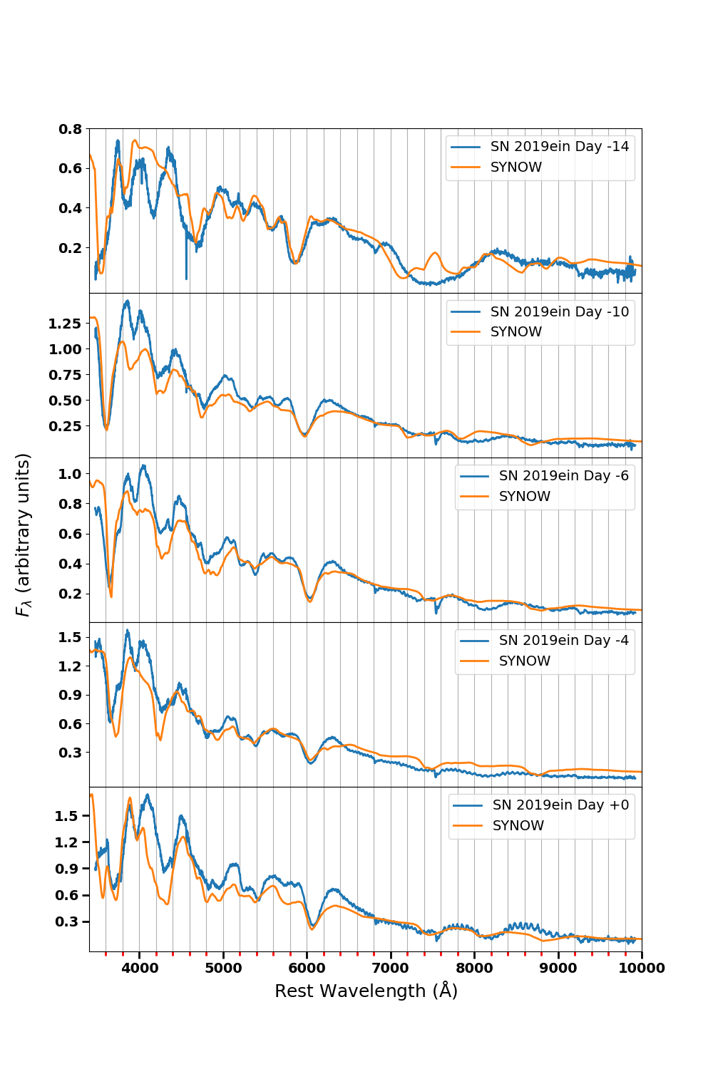
(a) SN 2019ein

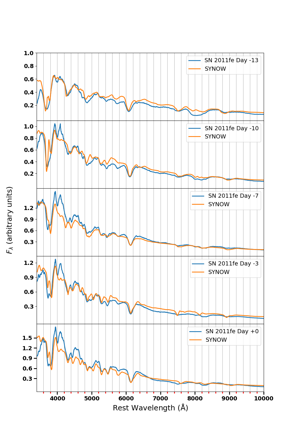
(b) SN 2011fe

Figure 1: SYNOW fits to pre-maximum spectra of SNe 2019ein and 2011fe.

3 Discussion

3.1 Interpretation of Results

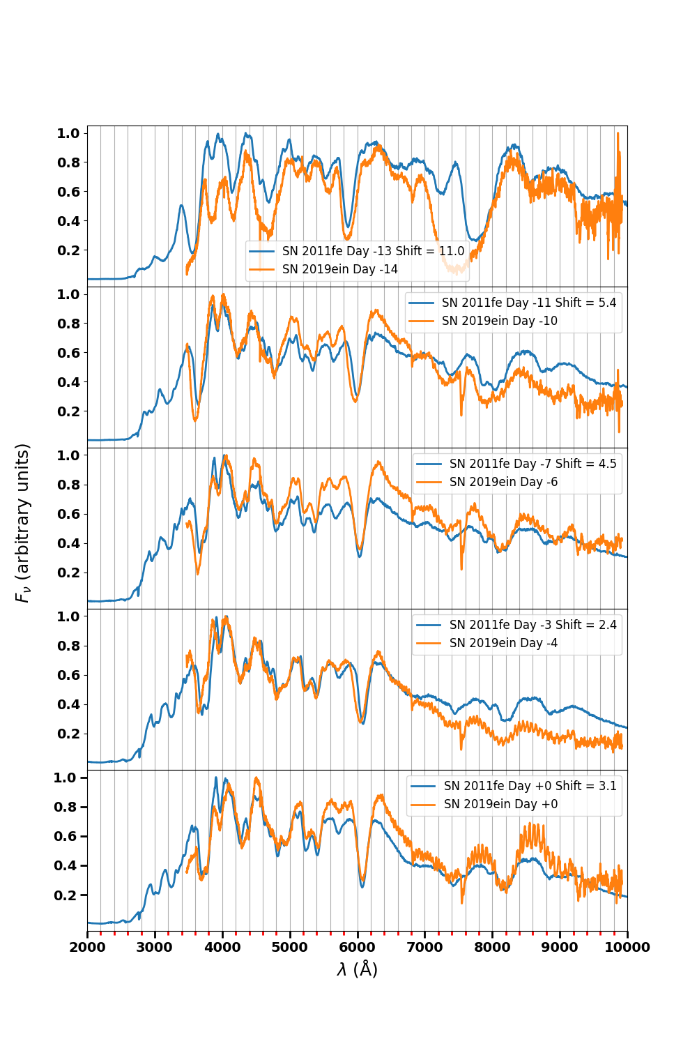
Figure 2: Comparison of of the observed SN 2019ein corrected to the rest wavelength with the observed spectra of SN 2011fe, where the SN 2011fe spectra have been blue shifted by the amounts indicated in the legend in units of $1000$ $\text{km}~{}\text{s}^{-1}$.

Figure 2 shows that simply blue-shifting the observed pre-maximum spectra of SN 2011fe to match the pre-maximum spectra of SN 2019ein shows remarkable alignment for almost all features. This similarity of the spectra is striking and indicates that SN 2019ein, up until maximum light, is physically (at least in terms of the total optical depth of the ions that produce the main spectral features), very similar to SN 2011fe, with the only difference being the shifted velocities.

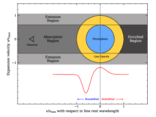
Figure 3: A cartoon illustrating the formation of P-Cygni line profiles. Adapted from Czekala (2011).

The formation of P-Cygni lines has been discussed for decades (see for example, Lucy, 1971; Surdej, 1979; Castor & Lamers, 1979; Wagenblast et al., 1983; Jeffery & Branch, 1990; Kasen et al., 2002, and references therein). Figure 3 illustrates the basic mechanism of P-Cygni line profile formation and clearly shows that the emission peak should be at the rest wavelength of the line for an isolated line that has opacity throughout the line forming region.

Yet, Pellegrino et al. (2020) noted that in SN 2019ein the emission peaks were shifted by up to $10,000$ $\text{km}~{}\text{s}^{-1}$ and demonstrated that a detached Si ii component (offset from the photosphere by $2500$ $\text{km}~{}\text{s}^{-1}$) could reproduce the Si ii 5970 and Si ii 6355 features at day $-10$. Therefore, since both the absorption and emission peaks of Si ii $\lambda 6355$ are shifted in the observed SN 2019ein spectra, this indicates that the community’s understanding of how P-Cygni lines form, as shown in Figure 3, may be incomplete and requires further investigation.

Blue-shifted emission features observed in Type II supernovae have been suggested to arise from steep density profiles (Dessart & Hillier, 2005, 2011; Anderson et al., 2014). However, in SNe II the Balmer lines are so strongly NLTE that SYNOW does a poor job of modeling them. Dessart & Hillier (2005) and Blondin et al. (2006) argue that the blueshifted P-Cygni emission is due to an optically thick continuum near the photosphere. Since SYNOW, a pure line-scattering code neglects continuum effects, we can not address this. Nevertheless, as shown below, we obtain very good fits to the observed line profiles, so we can infer the velocity extent of the ions that produce the observed features.

Turning our attention to single P-Cygni profile formation, Figure 4(a) shows that a high velocity photospheric P-Cygni profile can not simply be mimicked by just Doppler shifting a lower velocity photospheric P-Cygni profile. Because the prominent emission components are also blue-shifted, when the full line profile is Doppler shifted, the emission component of the shifted low-velocity now appears in the absorption trough of the high velocity line. While in the true SYNOW formulation absorptions trump emissions, it is important to understand that even though the observations can be made to match nearly perfectly by a Doppler shift, an individual P-Cygni feature can not.

A simple density variation does not remedy this problem either (see again Figure 4(a)). We show a moderate density profile, $\rho\propto v^{-7}$ compared to a moderately steep density profile, $\rho\propto v^{-14}$. The density variation mostly affects the slope of the line shape that connects the blue-shift P-Cygni absorption trough to the P-Cygni emission peak. In both cases (whether there is a moderate or steep density gradient), the shifted emission peak is clearly visible in the absorption trough of the higher velocity P-Cygni feature, which is not seen in the observations. In fact, Figure 2 shows that the shifted SN 2011fe spectrum matches up with that of SN 2019ein quite well. Thus, the line formation in SN 2019ein and SN 2011fe must be more complex than just a simple Doppler shift of photospheric P-Cygni lines, since changing the density gradient in the SYNOW framework does not affect the position of the emission peak — that is, the emission peak is formed at zero velocity (see Figure 3).

Figure 4(b) shows the components of the SYNOW fits of the Si ii $\lambda 6355$ line at the earliest epoch for both supernovae. In the case of SN 2011fe the photospheric velocity is $v_{\text{phot}}=14,000$ $\text{km}~{}\text{s}^{-1}$. There is a photospheric component to the Si ii feature and a detached component, $v_{\text{min}}=17,000$ $\text{km}~{}\text{s}^{-1}$, with equal values of $\tau=4$. For SN 2019ein the photospheric velocity is $v_{\text{phot}}=18,000$ $\text{km}~{}\text{s}^{-1}$. There are two detached components to the Si ii feature: $v_{\text{min}}=25,000$ $\text{km}~{}\text{s}^{-1}$ ($\tau=32$) and $v_{\text{min}}=30,000$ $\text{km}~{}\text{s}^{-1}$ ($\tau=5$). By maximum light, for SN 2011fe, $v_{\text{phot}}$ has dropped to $8,000$ $\text{km}~{}\text{s}^{-1}$ and the detached feature has $v_{\text{min}}=11,250$ $\text{km}~{}\text{s}^{-1}$. Again both components are of equal strength, $\tau=2$. For SN 2019ein, $v_{\text{phot}}$ has dropped to $15,200$ $\text{km}~{}\text{s}^{-1}$; there is now a photospheric component and a detached feature with $v_{\text{min}}=17,000$ $\text{km}~{}\text{s}^{-1}$. Again both components are of equal strength, $\tau=8$. Thus, even at maximum light SN 2019ein is significantly faster in the Si ii photosphere than SN 2011fe. Figure 5 shows the values obtained for the photospheric and detached components of the Si ii and Ca ii. The general trend is clear: the photospheric and detached components of SN 2019ein are almost universally faster than those of SN 2011fe. Nevertheless, when shifted, the features are extremely similar. This suggests that the burning in both supernovae produces similar amounts of these elements even though the density structure is quite different.

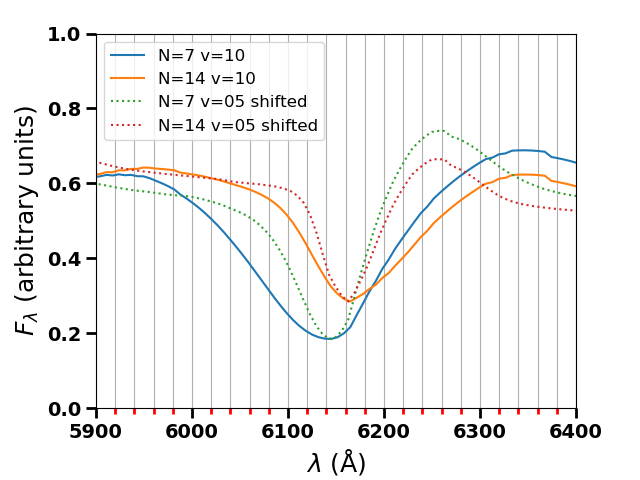
(a)

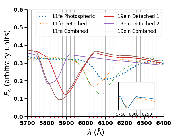
(b)

Figure 4: Panel (a) shows a P-Cygni line with $v_{\text{phot}}=10,000$ $\text{km}~{}\text{s}^{-1}$ compared to a P-Cygni line with $v_{\text{phot}}=5,000$ $\text{km}~{}\text{s}^{-1}$ that has been blue shifted by $5000$ $\text{km}~{}\text{s}^{-1}$. Two density profiles are chosen: $\rho\propto v^{-7}$ and $\rho\propto v^{-14}$. Clearly a simple photospheric P-Cygni profile does not shift in order to match the observations of SNe 2011fe and 2019ein. Panel (b) shows that detached P-Cygni lines can mimic the observed spectra. The photospheric velocity, $v_{\text{ph}}$, for the 11fe fit is 14,000 $\text{km}~{}\text{s}^{-1}$, the maximum velocity, $v_{\text{max}}$ is 40,000 $\text{km}~{}\text{s}^{-1}$, the detatched velocity, $v_{\text{detach}}$ is 17,000 $\text{km}~{}\text{s}^{-1}$. For 19ein $v_{\text{ph}}=18,000$ $\text{km}~{}\text{s}^{-1}$, $v_{\text{max}}=50,000$ $\text{km}~{}\text{s}^{-1}$, $v_{\text{detach}{{}_{1}}}=25,000$ $\text{km}~{}\text{s}^{-1}$, and $v_{\text{detach}{{}_{2}}}=30,000$ $\text{km}~{}\text{s}^{-1}$. The inset shows the comparison of the total combined SYNOW 19ein feature (solid blue line) with the total combined 11fe SYNOW feature blueshifted by $10,500$ $\text{km}~{}\text{s}^{-1}$ (dotted red line).

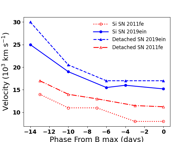
(a)

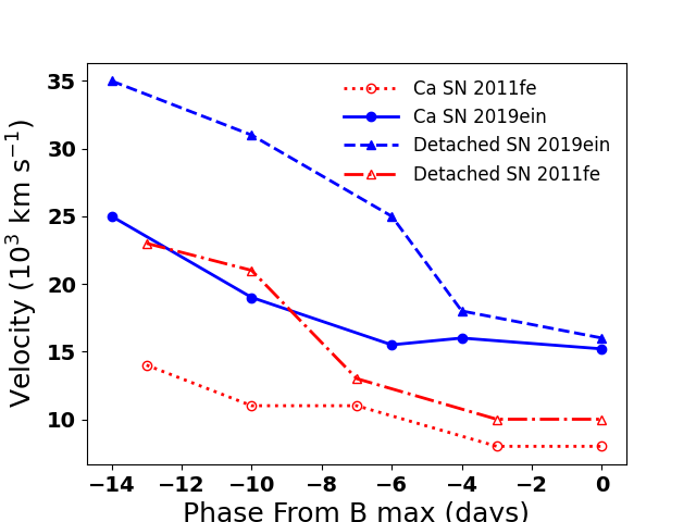
(b)

Figure 5: SYNOW velocities of Si ii (left) and Ca ii (right) obtained for SN 2019ein compared to those of SN 2011fe.

3.2 Comparison to Explosion Models

Blondin et al. (2015) modeled the light curve and spectral evolution of SN 2002bo, using delayed-detonation model DDC15 from Blondin et al. (2013). The transition to a detonation was triggered at $\rho=1.8\times 10^{7}$ g cm^-3 and the central density of the WD was $\rho_{c}=2.6\times 10^{9}$ g cm^-3. The model does a good job of reproducing the light curves and spectra of SN 2002bo. However, Pellegrino et al. (2020) showed that while DDC15 does a good job of fitting SN 2019ein spectra after about day -10, the whole P-Cygni structure of the features of SN 2019ein is blueshifted with respect to DDC15 at day -14, just the effect we focus on here.

Lentz et al. (2001) modeled SN 1984A using the delayed detonation models DD21c of Höflich et al. (1998) and CS15DD3 of (Iwamoto et al., 1999). Both models do a good job of reproducing the spectra of SN 1984A. Similarly Baron et al. (2015) modeled the evolution of the spectra of SN 2011fe using the delayed detonation model Z23 of Höflich et al. (2002), the transition density was triggered at $\rho=2.3\times 10^{7}$ g cm^-3 and the central density was $\rho_{c}=2.0\times 10^{9}$ g cm^-3.

Baron et al. (2012) model the BL SN 2001ay in detail using the pulsating delayed detonation model PDD_11b. The pulsating delayed detonation mechanism occurs when the deflagration is quenched, prior to the white dwarf becoming unbound, during the contraction phase a detonation can occur (Khokhlov et al., 1993). Besides being a clear BL, SN 2001ay is an extremely slow decliner, whose brightness is less than that which would be predicted by the Phillips relation. Nevertheless, the synthetic spectra do a very good job of reproducing the observed Si ii line profiles, particularly with respect to the positions of the minimum velocity and the emission maximum.

Figure 6(a) shows the density profiles of our previously calculated models for SN 2011fe (Z23), SN 1984A (DD21c), and SN 2001ay (PDD_11b). While the pulsational delayed-detonation model clearly displays a shell as expected, the obvious differences between the BL models and the CN model are: higher densities at higher velocities for the BL models; significant carbon depletion at high velocities for the BL models; and a more extended ${}^{56}{\text{Ni}}$ distribution for the BL models although the extremely extended ${}^{56}{\text{Ni}}$ distribution for PDD_11b is a particular feature that was needed to reproduce the observed light curve shape of SN 2001ay (Baron et al., 2012). It is interesting to note that most BL and HV SNe Ia have no observed C ii absorption at early times (see, for example, Parrent et al., 2012), with the notable exception of SN 2019ein.

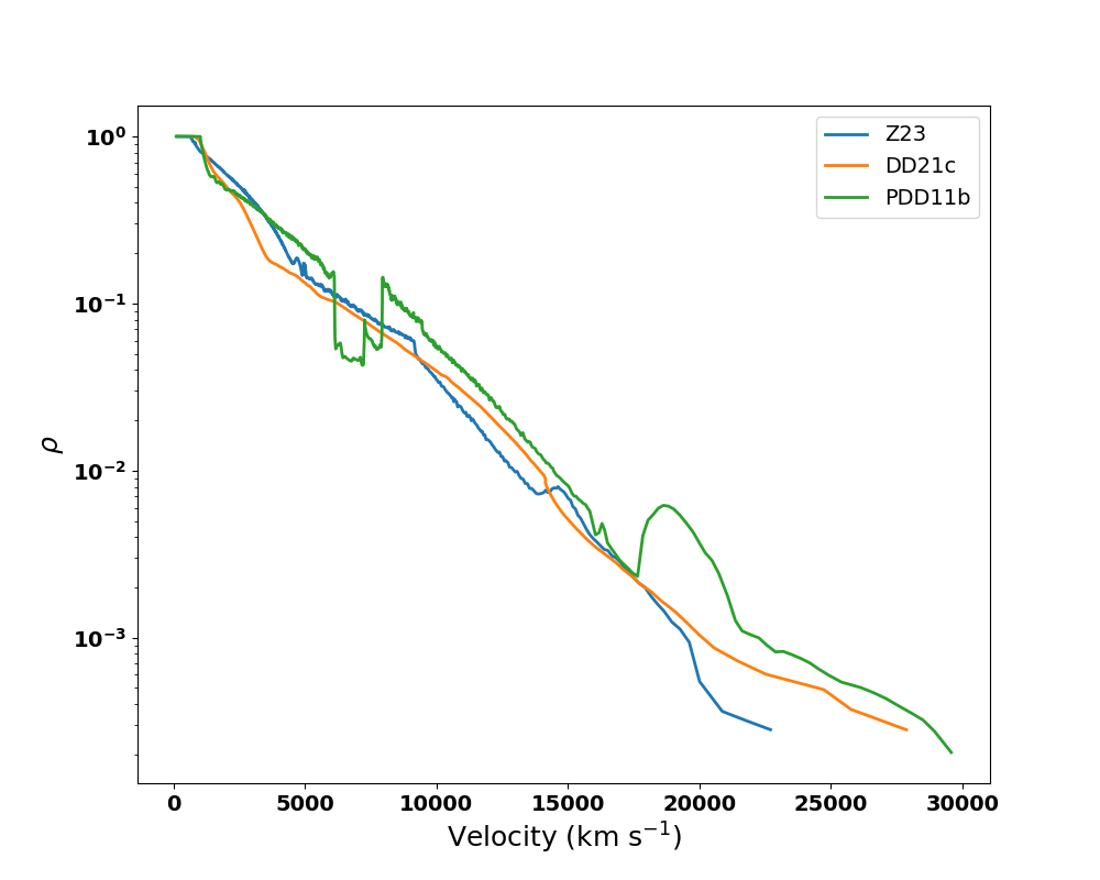
(a)

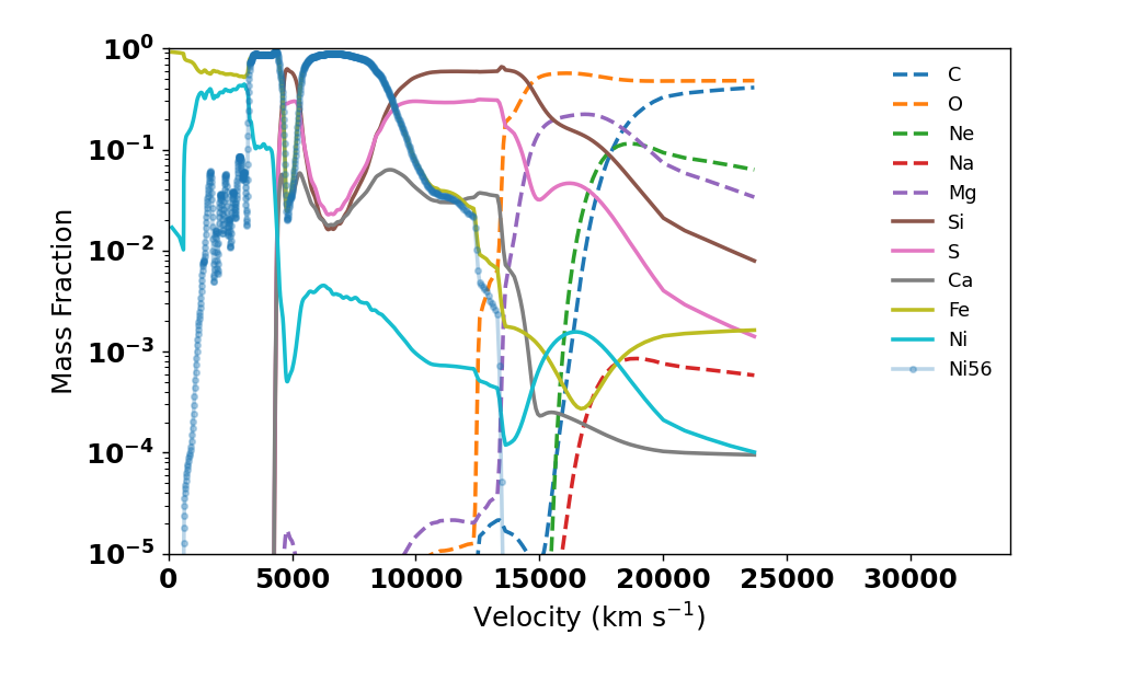
(b) Z23

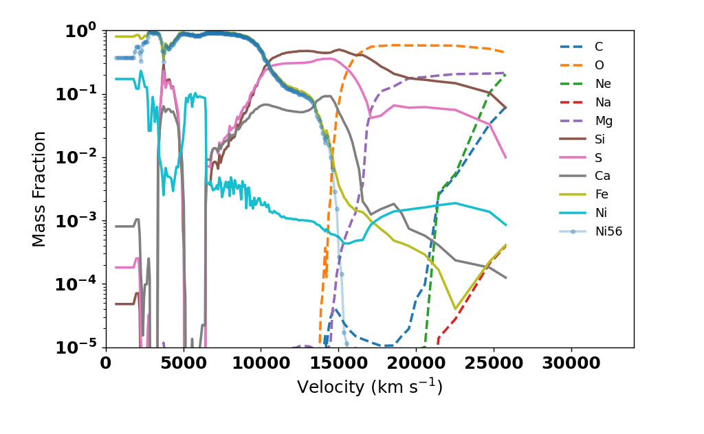
(c) DD21c

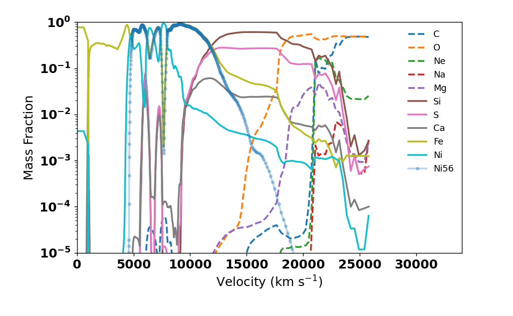
(d) PDD11b

Figure 6: The density and composition profiles of the two delayed detonation models DD21c, Z23, and the pulsational delayed-detonation model PDD_11b (used to model SN 1984A, SN 2011fe, and SN 2001ay, respectively) are compared. All elements except ${}^{56}{\text{Ni}}$ are displayed at $t=\infty$, while ${}^{56}{\text{Ni}}$ is given at $t=0$.

In general, high expansion velocities can be formed in two ways. First, by the redistribution of the kinetic energy by means of a shell interaction, namely the ejecta run into a dense circumstellar medium (CSM) shell produced during a large amplitude pulsational phase; the characteristics of this CSM shell interaction are slow-rising-red lightcurves and early blue line wings with a almost linear relation between the blue edge of the velocities of quasi-statistical equilibrium (QSE) elements and the mass of the shell (Khokhlov et al., 1992; Hoeflich & Khokhlov, 1996; Quimby et al., 2006). The separation in the production of a high velocity shell between classical delayed-detonation and pulsational delayed-detonation is not a bifurcation, but rather a continuum with low mass, low amplitude pulsations appearing to be most common (Hoeflich, 2017).

The second mechanism is related to an increase of nuclear energy as a result of the C/O ratio produced during the central He-burning under He-depleted conditions as suggested for SN2001ay (Baron et al., 2012). Within the framework of delayed-detonation models, the results are high velocity wings in Si as commonly observed in SNe Ia, but also overall broad lines in features produced in QSE. The size of the He-burning zone depends on the main-sequence mass of the progenitor and ranges between $0.2-1.0$ ${\text{M}_{\odot}}$ for a MS mass of $1-8$ ${\text{M}_{\odot}}$ (Domínguez et al., 2001). Thus, we may expect a continuum of expansion velocities for BL SNe.

For SN 2019ein, the outermost layers show C/O rich mixtures, but also a wing of Si extending up to about 24,000 $\text{km}~{}\text{s}^{-1}$ (Patra et al., 2022) implying a upper mass limit of a shell to about $5\times 10^{-2}$ ${\text{M}_{\odot}}$ (Yang et al., 2020). Thus, this suggests that SN 2019ein falls in the continuum of low mass, low amplitude pulsations (Hoeflich, 2017).

3.3 The BL Sample

We collected spectra of BL SNe that were obtained prior to maximum light in the $B$-band, including: SNe 1984A (Branch, 1987; Barbon et al., 1989), 1997bq (Blondin et al., 2012), 2001ay (Krisciunas et al., 2011), 2002bo (Benetti et al., 2004), 2002dj (Pignata et al., 2008), 2004dt (Altavilla et al., 2007), 2006X (Wang et al., 2008), 2010ev (Gutiérrez et al., 2016), and 2019ein (Kawabata et al., 2020; Pellegrino et al., 2020). Figure 7 shows the S ii and Si ii regions of these supernova spectra. All of the BL/High-velocity SNe that we have examined show that the P-Cygni emission peak of Si ii $\lambda 6355$ is blueshifted in the epochs -6 – -2 days, thus this could serve as a simple classification criterion (Figure 7). The validity of this indicator as a classification criterion will be the subject of future work. If we use the preferred redshift suggested by NED for the SN 2002bo host NGC 3190, $z=0.00437$, ($v$ heliocentric = 1310 $\text{km}~{}\text{s}^{-1}$ Leisman et al., 2016), the peak of SN 2002bo is not blue-shifted. This seems unlikely that the class defining -4 day spectrum of SN 2002bo would be the one exception, so therefore we have adopted the higher value $v$ heliocentric = 1698 $\text{km}~{}\text{s}^{-1}$ (Mould et al., 2000). NGC 3190 is a very nearby, nearly edge-on spiral, so a peculiar velocity of 300 $\text{km}~{}\text{s}^{-1}$ in the galaxy for the supernova would not be surprising.

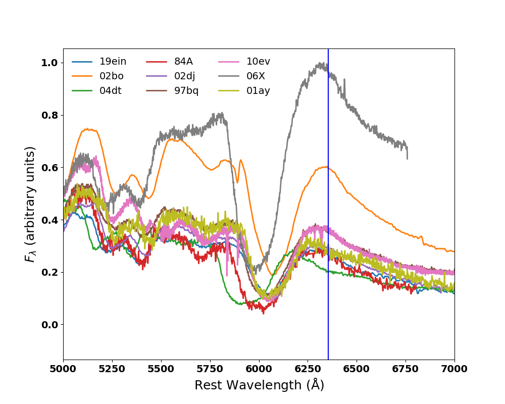
Figure 7: The spectra of BL SNe Ia observed at days -2 – -6 with respect to $B$-maximum. The dates are (-5, -6, -2, -4, -5, -2, -6, -4, and -4) for (84A, 97bq, 01ay, 02bo, 02dj, 04dt, 06X, 10ev, and 19ein), respectively. See Section 3.3 for the original sources of these spectra. With the exception of SN 2002bo, all of the BL/High-velocity SNe show that the P-Cygni emission peak of Si ii $\lambda 6355$ is blueshifted in the epochs -2 – -6, thus this could serve as a simple classification criterion.

Figure 8 shows the velocities of the Si II absorption trough minimum for a set of BL SNe Ia. This figure shows behavior very similar to that found by Wang et al. (2009) where there is a continuum of velocities with SN 2002bo being one of the lower velocity SN and SN 2006X being one of the higher velocity SN. This is consistent with the discussion above that suggests in the framework of delayed detonation, a continuum of line velocities is expected. Note that even at 10–15 days past maximum light, the Si velocities have not fallen to the values of SN 2011fe, clearly indicating that even though the nucleosynthetic products of BL SNe Ia are nearly identical to that of CN, BL SNe Ia are a distinct sub-class.

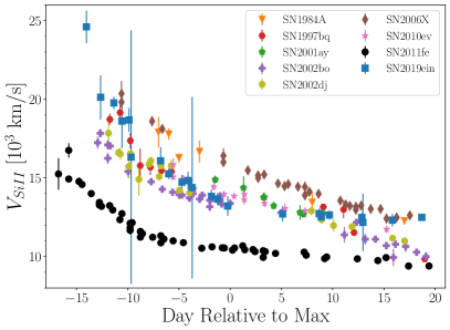
Figure 8: The measured velocity of the the Si ii $\lambda 6355$ absorption trough minimum for the set of BL-SNe Ia, including SNe 1984A (Branch, 1987; Barbon et al., 1989), 1997bq (Blondin et al., 2012), 2001ay (Krisciunas et al., 2011), 2002bo (Benetti et al., 2004), 2002dj (Pignata et al., 2008), 2006X (Wang et al., 2008), 2010ev (Gutiérrez et al., 2016), and 2019ein (Kawabata et al., 2020; Pellegrino et al., 2020). Measurements of SN 2011fe (Parrent et al., 2012; Pereira et al., 2013) are also shown for comparison.

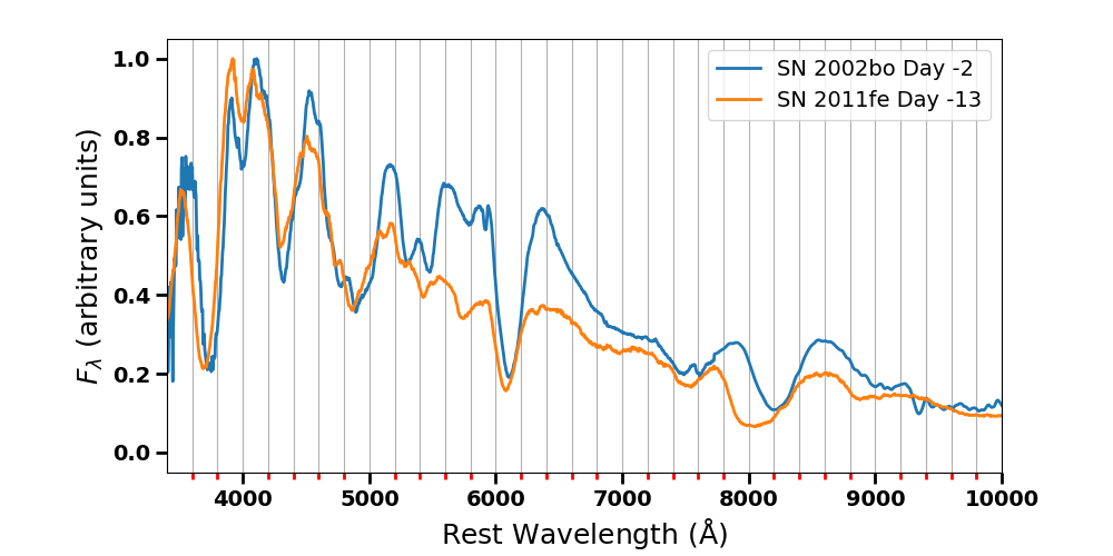
(a)

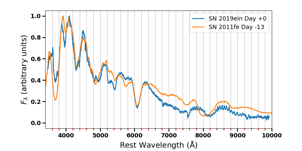
(b)

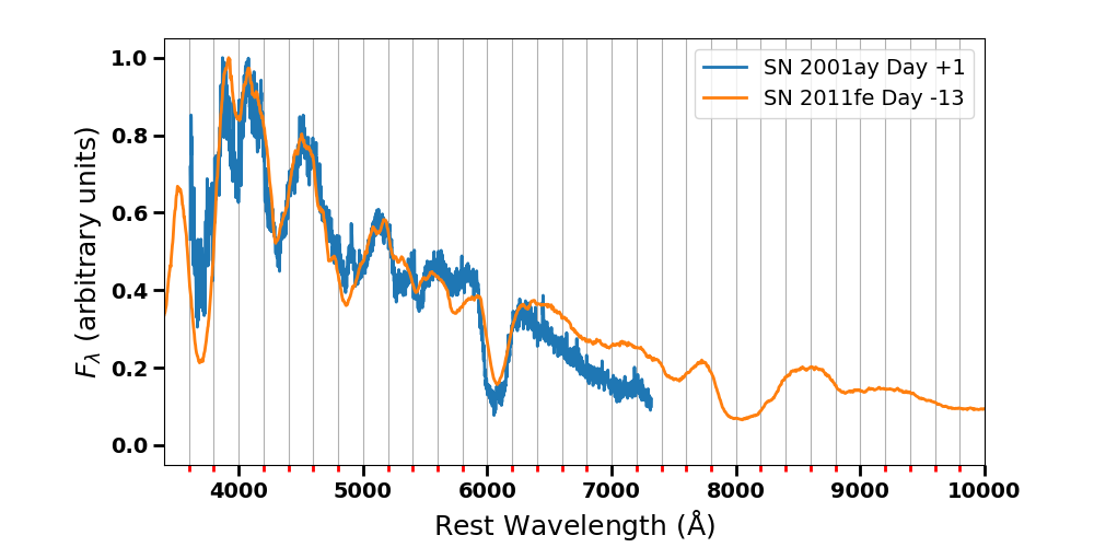
(c)

Figure 9: Panel (a) compares SN 2002bo at day -2 to SN 2011fe at day -13. Panel (b) compares SN 2019ein at day +0 to SN 2011fe at day -13. Panel (c) compares SN 2001ay at day +1 to SN 2011fe at day -14. A broad variety of BL supernovae have observed spectra near maximum light are well matched by early-time spectra of the CN SN 2011fe, suggesting that the high observed velocities are truly due to variations in the outermost part of the ejecta of BL SNe.

Figure 9 shows that for a broad variety of BL/High-Velocity/02bo-like supernovae that the observed spectra near maximum light are well matched by early-time spectra of the CN SN 2011fe. Interestingly, the poorest match is for the class defining SN 2002bo, where the Ca IR triplet of SN 2011fe extends to higher velocity than that of SN 2002bo and the strength of the Si ii lines is not as well-matched as it is for SN 2019ein and SN 2001ay. Unfortunately, the maximum light spectrum of SN 2001ay does not extend to the Ca IR triplet, but the fit in the blue is remarkable.

Xi et al. (2022) found that the high velocities of SN 2019ein are due to asymmetries, however SN 2019ein shows no evidence for polarization (Patra et al., 2022) indicating that there are no very strong asymmetries. In the delayed detonation framework, CN SNe Ia appear to arise from off-center detonations (DerKacy et al., 2023). In looking for the progenitor/explosion scenario one should note that BL occur preferentially in luminous galaxies (Folatelli et al., 2013; Morrell et al., 2023).

3.4 Summary

Our direct analysis shows that blue-shifted P-Cygni profiles can be produced in the SYNOW framework by high velocity photospheric features coupled with one or more detached component. This result is consistent with detailed models of SN 1984A (Lentz et al., 2001) and SN 2001ay (Baron et al., 2012) using a delayed-detonation and pulsational delayed-detonation model respectively, showing that shell like structures occur in the near-$M_{\text{Ch}}$ framework. The modeling shows that the outer compositions and ionization stages of the core-normal SN 2011fe and the broad-line SN 2019ein are extremely similar, except that the features of the BL SN are blue-shifted with respect to those of the CN SN. This illustrates the fact that the progenitor compositions must be very similar and the burning leads to a so-called stellar amnesia (Höflich, 2006). Our models indicate the outer parts of SN 2019ein likely form in a higher-density environment, something like a shell, but the effects of the shell is mostly dissipated by the time of maximum light. Future work should focus on a comparative study of BL SNe Ia and CN in order to probe the progenitor variations between these two Branch groups.

Data Availability

The observed spectra are available from TNS, WISeREP (Yaron & Gal-Yam, 2012) and the SYNOW fits are available from the authors upon request.

References

- Altavilla et al. (2007) Altavilla G., et al., 2007, A&A, 475, 585
- Anderson et al. (2014) Anderson J. P., et al., 2014, MNRAS, 441, 671
- Barbon et al. (1989) Barbon R., Iijima T., Rosino L., 1989, A&A, 220, 83
- Baron et al. (2012) Baron E., Höflich P., Krisciunas K., Dominguez I., Khokhlov A. M., Phillips M. M., Suntzeff N., Wang L., 2012, ApJ, 753, 105
- Baron et al. (2015) Baron E., et al., 2015, MNRAS, 454, 2549
- Benetti et al. (2004) Benetti S., et al., 2004, MNRAS, 348, 261
- Benetti et al. (2005) Benetti S., et al., 2005, ApJ, 623, 1011
- Blondin et al. (2006) Blondin S., et al., 2006, AJ, 131, 1648
- Blondin et al. (2012) Blondin S., et al., 2012, AJ, 143, 126
- Blondin et al. (2013) Blondin S., Dessart L., Hillier D. J., Khokhlov A. M., 2013, MNRAS, 429, 2127
- Blondin et al. (2015) Blondin S., Dessart L., Hillier D. J., 2015, MNRAS, 448, 2766
- Bloom et al. (2012) Bloom J. S., et al., 2012, ApJ, 744, L17
- Branch (1987) Branch D., 1987, ApJ, 316, L81
- Branch et al. (2006) Branch D., et al., 2006, PASP, 118, 560
- Brown et al. (2012) Brown P. J., et al., 2012, ApJ, 753, 22
- Burke et al. (2019) Burke J., Arcavi I., Howell D. A., Hiramatsu D., McCully C., 2019, Transient Name Server AstroNote, 8, 1
- Burns et al. (2014) Burns C. R., et al., 2014, ApJ, 789, 32
- Burrow et al. (2020) Burrow A., et al., 2020, ApJ, 901, 154
- Castor & Lamers (1979) Castor J. I., Lamers H. J. G. L. M., 1979, ApJS, 39, 481
- Czekala (2011) Czekala I., 2011, The Variability of Massive Stars, https://astrobites.org/2011/01/26/variability-of-massive-stars/
- DerKacy et al. (2020) DerKacy J. M., Baron E., Branch D., Hoeflich P., Hauschildt P., Brown P. J., Wang L., 2020, ApJ, 901, 86
- DerKacy et al. (2023) DerKacy J. M., et al., 2023, ApJ, 945, L2
- Dessart & Hillier (2005) Dessart L., Hillier D. J., 2005, A&A, 437, 667
- Dessart & Hillier (2011) Dessart L., Hillier D. J., 2011, MNRAS, 410, 1739
- Dessart et al. (2014) Dessart L., Blondin S., Hillier D. J., Khokhlov A., 2014, MNRAS, 441, 532
- Domínguez et al. (2001) Domínguez I., Höflich P., Straniero O., 2001, ApJ, 557, 279
- Dong et al. (2022) Dong Y., et al., 2022, ApJ, 934, 102
- Fisher (2000) Fisher A. K., 2000, PhD thesis, University of Oklahoma, Norman
- Folatelli et al. (2013) Folatelli G., et al., 2013, ApJ, 773, 53
- Gutiérrez et al. (2016) Gutiérrez C. P., et al., 2016, A&A, 590, A5
- Hoeflich (2017) Hoeflich P., 2017, in Alsabti A. W., Murdin P., eds, , Handbook of Supernovae. Springer, Berlin, p. 1151, doi:10.1007/978-3-319-21846-5_56
- Hoeflich & Khokhlov (1996) Hoeflich P., Khokhlov A., 1996, ApJ, 457, 500
- Hoeflich et al. (1995) Hoeflich P., Khokhlov A. M., Wheeler J. C., 1995, ApJ, 444, 831
- Höflich (2006) Höflich P., 2006, Nuclear Phys. A, 777, 579
- Höflich et al. (1998) Höflich P., Wheeler J. C., Thielemann F. K., 1998, ApJ, 495, 617
- Höflich et al. (2002) Höflich P., Gerardy C. L., Fesen R. A., Sakai S., 2002, ApJ, 568, 791
- Hoyle & Fowler (1960) Hoyle F., Fowler W. A., 1960, ApJ, 132, 565
- Hsiao et al. (2013) Hsiao E. Y., et al., 2013, ApJ, 766, 72
- Hsiao et al. (2019) Hsiao E. Y., et al., 2019, PASP, 131, 014002
- Iben & Tutukov (1984) Iben I. J., Tutukov A. V., 1984, ApJS, 54, 335
- Iwamoto et al. (1999) Iwamoto K., Brachwitz F., Nomoto K., Kishimoto N., Umeda H., Hix W. R., Thielemann F.-K., 1999, ApJS, 125, 439
- Jeffery & Branch (1990) Jeffery D. J., Branch D., 1990, in Wheeler J. C., Piran T., Weinberg S., eds, Jerusalem Winter School for Theoretical Physics Vol. 6, Supernovae. p. 149
- Kasen et al. (2002) Kasen D., Branch D., Baron E., Jeffery D., 2002, ApJ, 565, 380
- Kashi & Soker (2011) Kashi A., Soker N., 2011, MNRAS, 417, 1466
- Kawabata et al. (2020) Kawabata M., et al., 2020, ApJ, 893, 143
- Khokhlov (1991) Khokhlov A. M., 1991, A&A, 245, 114
- Khokhlov et al. (1992) Khokhlov A., Mueller E., Hoeflich P., 1992, A&A, 253, L9
- Khokhlov et al. (1993) Khokhlov A., Mueller E., Hoeflich P., 1993, A&A, 270, 223
- Krisciunas et al. (2011) Krisciunas K., et al., 2011, AJ, 142, 74
- Krisciunas et al. (2017) Krisciunas K., et al., 2017, AJ, 154, 211
- Kwok et al. (2023) Kwok L. A., et al., 2023, ApJ, 944, L3
- Leisman et al. (2016) Leisman L., Haynes M. P., Giovanelli R., Józsa G., Adams E. A. K., Hess K. M., 2016, MNRAS, 463, 1692
- Lentz et al. (2001) Lentz E. J., Baron E., Branch D., Hauschildt P. H., 2001, ApJ, 547, 402
- Li et al. (2011) Li W., et al., 2011, Nature, 480, 348
- Liu et al. (2022) Liu C., et al., 2022, arXiv e-prints, p. arXiv:2209.04463
- Livne & Arnett (1995) Livne E., Arnett D., 1995, ApJ, 452, 62
- Lucy (1971) Lucy L. B., 1971, ApJ, 163, 95
- Maoz et al. (2014) Maoz D., Mannucci F., Nelemans G., 2014, ARA&A, 52, 107
- Mazzali et al. (2014) Mazzali P. A., et al., 2014, MNRAS, 439, 1959
- Mihalas (1978) Mihalas D., 1978, Stellar Atmospheres, 2nd edn. W. H. Freeman, New York
- Morrell et al. (2023) Morrell N., et al., 2023, ApJ, in preparation
- Mould et al. (2000) Mould J. R., et al., 2000, ApJ, 529, 786
- Nugent et al. (2011) Nugent P. E., et al., 2011, Nature, 480, 344
- Parrent et al. (2012) Parrent J. T., et al., 2012, ApJ, 752, L26
- Patra et al. (2022) Patra K. C., et al., 2022, MNRAS, 509, 4058
- Pellegrino et al. (2020) Pellegrino C., et al., 2020, ApJ, 897, 159
- Pereira et al. (2013) Pereira R., et al., 2013, A&A, 554, A27
- Phillips (1993) Phillips M. M., 1993, ApJ, 413, L105
- Phillips et al. (1999) Phillips M. M., Lira P., Suntzeff N. B., Schommer R. A., Hamuy M., Maza J., 1999, AJ, 118, 1766
- Phillips et al. (2019) Phillips M. M., et al., 2019, PASP, 131, 014001
- Pignata et al. (2008) Pignata G., et al., 2008, MNRAS, 388, 971
- Polin et al. (2019) Polin A., Nugent P., Kasen D., 2019, ApJ, 873, 84
- Quimby et al. (2006) Quimby R., Höflich P., Kannappan S. J., Rykoff E., Rujopakarn W., Akerlof C. W., Gerardy C. L., Wheeler J. C., 2006, ApJ, 636, 400
- Shen et al. (2018) Shen K. J., Kasen D., Miles B. J., Townsley D. M., 2018, ApJ, 854, 52
- Sobolev (1960) Sobolev V. V., 1960, Moving Envelopes of Stars. Harvard Univ. Press, Cambridge, MA
- Soker et al. (2014) Soker N., García-Berro E., Althaus L. G., 2014, MNRAS, 437, L66
- Surdej (1979) Surdej J., 1979, A&A, 73, 1
- Tonry et al. (2019) Tonry J., et al., 2019, Transient Name Server Discovery Report, 2019-907, 1
- Wagenblast et al. (1983) Wagenblast R., Bertout C., Bastian U., 1983, A&A, 120, 6
- Wang et al. (2008) Wang X., et al., 2008, ApJ, 675, 626
- Wang et al. (2009) Wang X., et al., 2009, ApJ, 699, L139
- Webbink (1984) Webbink R. F., 1984, ApJ, 277, 355
- Woosley & Weaver (1994) Woosley S. E., Weaver T. A., 1994, ApJ, 423, 371
- Xi et al. (2022) Xi G., et al., 2022, MNRAS, 517, 4098
- Yang et al. (2020) Yang Y., et al., 2020, ApJ, 902, 46
- Yaron & Gal-Yam (2012) Yaron O., Gal-Yam A., 2012, PASP, 124, 668
- Zhang et al. (2016) Zhang K., et al., 2016, ApJ, 820, 67