Deflated HeteroPCA: Overcoming the curse of ill-conditioning in heteroskedastic PCA

Abstract

This paper is concerned with estimating the column subspace of a low-rank matrix $\bm{X}^{\star}\in\mathbb{R}^{n_{1}\times n_{2}}$ from contaminated data. How to obtain optimal statistical accuracy while accommodating the widest range of signal-to-noise ratios (SNRs) becomes particularly challenging in the presence of heteroskedastic noise and unbalanced dimensionality (i.e., $n_{2}\gg n_{1}$). While the state-of-the-art algorithm HeteroPCA emerges as a powerful solution for solving this problem, it suffers from “the curse of ill-conditioning,” namely, its performance degrades as the condition number of $\bm{X}^{\star}$ grows. In order to overcome this critical issue without compromising the range of allowable SNRs, we propose a novel algorithm, called Deflated-HeteroPCA, that achieves near-optimal and condition-number-free theoretical guarantees in terms of both $\ell_{2}$ and $\ell_{2,\infty}$ statistical accuracy. The proposed algorithm divides the spectrum of $\bm{X}^{\star}$ into well-conditioned and mutually well-separated subblocks, and applies HeteroPCA to conquer each subblock successively. Further, an application of our algorithm and theory to two canonical examples — the factor model and tensor PCA — leads to remarkable improvement for each application.

Keywords: principal component analysis (PCA), heteroskedastic noise, the curse of ill-conditioning, factor models, tensor PCA

1 Introduction

In a diverse array of science and engineering applications, we are asked to identify a low-dimensional subspace that best captures the information underlying a large collection of high-dimensional data points, a classical problem that goes by the names of principal component analysis (PCA), subspace estimation, subspace tracking, among others (Johnstone and Paul,, 2018; Balzano et al.,, 2018; Chen et al., 2021b, ). A simple yet useful mathematical model is of the following form: imagine we have an unknown large-dimensional matrix $\bm{X}^{\star}\in\mathbb{R}^{n_{1}\times n_{2}}$ whose columns are high-dimensional vectors embedded in a $r$-dimensional subspace (so that $\bm{X}^{\star}$ has rank $r\ll\min\{n_{1},n_{2}\}$), and we seek to estimate the column space of $\bm{X}^{\star}$ from noisy observations:

$$\bm{Y}=\bm{X}^{\star}+\bm{E}\in\mathbb{R}^{n_{1}\times n_{2}},$$ (1)

where $\bm{E}$ stands for the noise matrix that contaminates the data. Despite decades-long research, there remain substantial challenges to handle heteroskedastic noise in high dimension, as we shall elaborate on below.

1.1 Challenges: unbalanced dimensionality and heteroskedasticity

How to achieve statistically efficient PCA in high dimension is an active research topic that has received much recent interest (Lounici,, 2014; Johnstone and Paul,, 2018; Cai et al.,, 2021; Zhu et al.,, 2019; Zhang et al.,, 2022; Agterberg et al.,, 2022). In this paper, we pay particular attention to the case where $n_{1}$ and $n_{2}$ are both enormous but highly unbalanced in the sense that $n_{1}\ll n_{2}$, a scenario that arises frequently in, say, covariance estimation (when there are many noisy samples available) and tensor estimation (when one has to matrice the tensor before estimation). Such unbalanced dimensionality gives rise to unique challenges not present in the complement case: as the signal-to-noise ratio (SNR) keeps decreasing, one might soon enter a regime where consistent estimation of $\bm{X}^{\star}$ is no longer infeasible but its column subspace — which is much smaller dimensional than the full matrix — remains estimatable. This regime is often considerably more challenging than the case with $n_{2}=O(n_{1})$, given that the majority of low-rank matrix estimation algorithms that directly attempt to estimate $\bm{X}^{\star}$ become completely off.

One natural strategy that comes into mind is thus to estimate the column subspace of $\bm{X}^{\star}$ by calculating the left singular subspace of the observed matrix $\bm{Y}$ (Cai and Zhang,, 2018; Abbe et al.,, 2020; Chen et al., 2021b, ), which we shall refer to as the vanilla SVD-based approach throughout. In the case with $n_{1}\ll n_{2}$, this simple scheme has only been shown to achieve the desired statistical performance when the noise matrix $\bm{E}$ is composed of i.i.d. entries, but falls short of effectiveness when handling heteroskedastic noise (i.e., the scenario where the variances of the entries of $\bm{E}$ are location-varying) (Zhang et al.,, 2022; Cai et al.,, 2021). This issue presents a hurdle to transferring this scheme from theory to practice, due to the ubiquity of heteroskedastic data in applications like social networks, recommendation systems, medical imaging, etc.

To mitigate this issue, at least two strategies have been proposed that attempt estimation by looking at the empirical covariance matrix (or gram matrix) $\bm{Y}\bm{Y}^{\top}$. Recognizing that large heteroskedastic noise might lead to significant bias in the diagonal of $\bm{Y}\bm{Y}^{\top}$ that distorts estimation, one natural remedy is to zero out (or sometimes rescale) the diagonal entries of $\bm{Y}\bm{Y}^{\top}$ before computing its eigendecomposition (Koltchinskii and Giné,, 2000; Lounici,, 2014; Florescu and Perkins,, 2016; Loh and Wainwright,, 2012; Montanari and Sun,, 2018; Elsener and van de Geer,, 2019; Cai et al.,, 2021; Ndaoud et al.,, 2021). A more refined iterative procedure called $\mathsf{HeteroPCA}$ was subsequently proposed by Zhang et al., (2022), which starts with the solution of diagonal-deleted PCA (cf. (10)) and alternates between:

• imputing the diagonal entries of $\bm{X}^{\star}\bm{X}^{\star\top}$;

• computing the rank-$r$ eigenspace of $\bm{Y}\bm{Y}^{\top}$ with its diagonal replaced by the imputed values.

See Section 3 for precise descriptions. In both theory and numerical experiments, this iterative paradigm yields enhanced performance compared to diagonal-deleted PCA (Zhang et al.,, 2022; Yan et al.,, 2021).

1.2 The curse of ill-conditioning

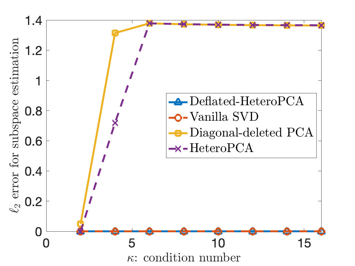
(a) Noiseless case

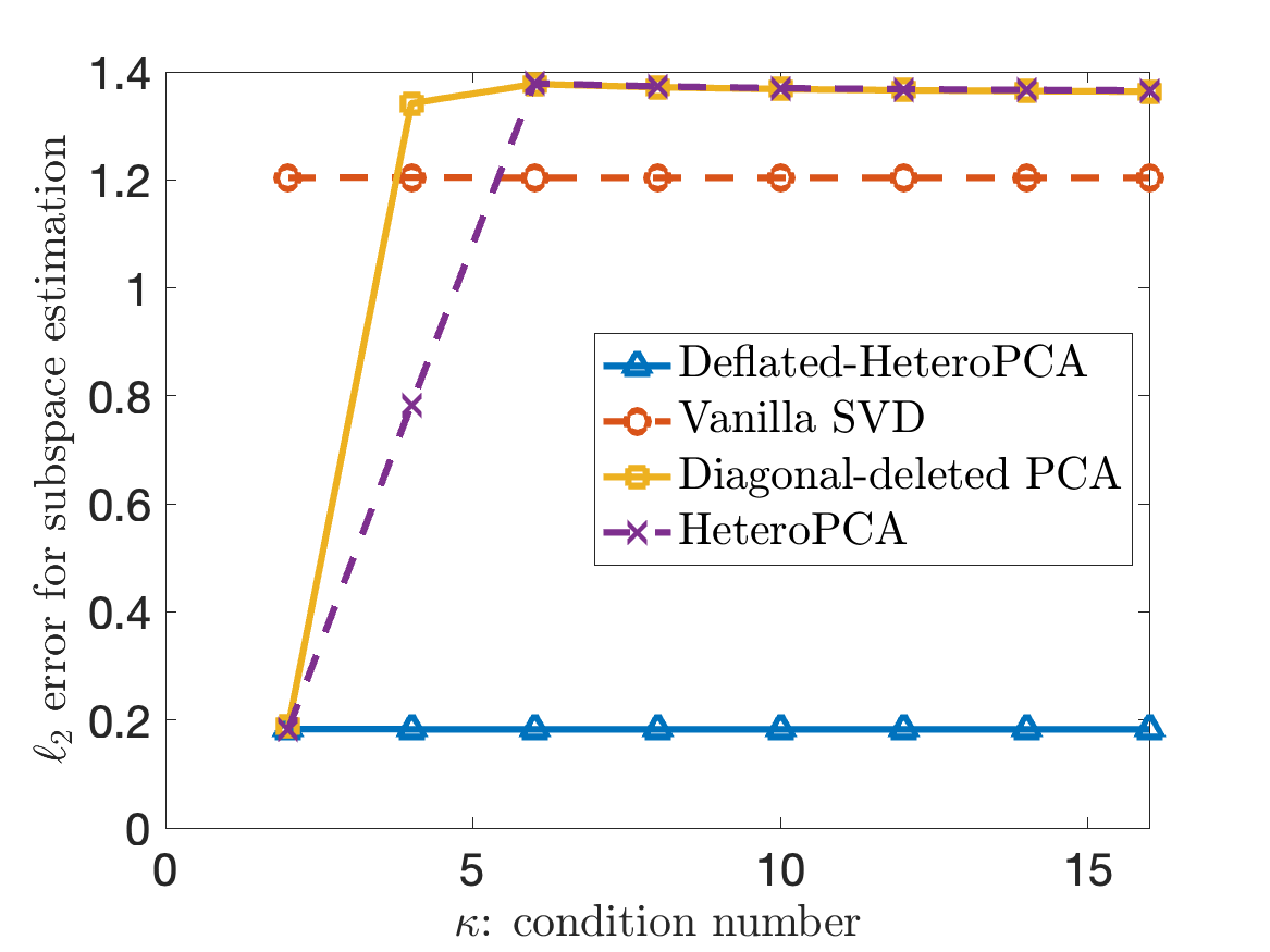
(b) Noisy case

Figure 1: Subspace estimation error vs. condition number $\kappa$ of $\bm{\Sigma}^{\star}$. Here, we set $r=2,n_{1}=200$ and $n_{2}=40,000$. The truth $\bm{X}^{\star}=\bm{U}^{\star}\bm{\Sigma}^{\star}\bm{V}^{\star\top}$ has rank 2 with $\bm{U}^{\star}\in\mathcal{R}^{n_{1}\times 2}$ and $\bm{V}^{\star}\in\mathcal{R}^{n_{2}\times 2}$ generated randomly. Plot (a) represents the noiseless case ($\bm{E}=\bm{0}$). In Plot (b), we choose the two singular values of $\bm{X}^{\star}$ as $\sigma_{1}^{\star}=\kappa\sigma_{2}^{\star}$ and $\sigma_{2}^{\star}=200$, generate $\{\omega_{i}\}_{1\leq i\leq n_{1}}$ independently from $\mathsf{Unif}([0,2])$, and draw the entries of $\bm{E}=[E_{i,j}]_{1\leq i\leq n_{1},1\leq j\leq n_{2}}$ independently such that $E_{i,j}\sim\mathcal{N}(0,\omega_{i}^{2})$. We compare multiple subspace estimators here, where $\mathsf{HeteroPCA}$ is run with 100 iterations. For each estimator $\widehat{\bm{U}}$, we compute the spectral-norm-based error $\|\widehat{\bm{U}}\bm{R}_{\widehat{\bm{U}}}-\bm{U}^{\star}\|$ as $\kappa$ varies, where $\bm{R}_{\widehat{\bm{U}}}=\mathop{\rm arg\min}_{\bm{R}\in\mathcal{O}^{r,r}}\|\widehat{\bm{U}}\bm{R}-\bm{U}^{\star}\|_{{\mathrm{F}}}$; the results are averaged over 50 independent runs.

Nevertheless, one drawback stands out when running either diagonal-deleted PCA or $\mathsf{HeteroPCA}$ in practice; that is, both algorithms become ineffective as the condition number of $\bm{X}^{\star}$ (when restricted to its non-zero singular values) grows. Let us illustrate this point more clearly via numerical experiments.

• (Numerical example) Consider the case where the unknwon signal $\bm{X}^{\star}$ has rank $r=2$ and obeys $\bm{X}^{\star}=\bm{U}^{\star}\bm{\Sigma}^{\star}\bm{V}^{\star\top},$ where the columns of $\bm{U}^{\star}\in\mathbb{R}^{n_{1}\times 2}$ (resp. $\bm{V}^{\star}\in\mathbb{R}^{n_{1}\times 2}$) are the two left (resp. right) singular vectors of $\bm{X}^{\star}$, and $\bm{\Sigma}^{\star}\in\mathbb{R}^{2\times 2}$ is a diagonal matrix composed of the two singular values $\sigma_{1}^{\star}\geq\sigma_{2}^{\star}>0$ of $\bm{X}^{\star}$. Denote by $\kappa=\sigma_{1}^{\star}/\sigma_{2}^{\star}$ the condition number of $\bm{\Sigma}^{\star}$. We conduct a series of experiments based on randomly generated $\bm{X}^{\star}$ with $n_{2}\gg n_{1}$, as detailed in the caption of Figure 1. As illustrated in Figure 1, when $\kappa$ is not too large, both diagonal-deleted PCA and HeteroPCA fail to return reliable estimates of the subspace $\bm{U}^{\star}$, even in the noiseless case (i.e., $\bm{E}=0$).

In summary, both diagonal-deleted PCA and HeteroPCA suffer from the “curse of ill-conditioning”, namely, they might lead to grossly incorrect subspace estimates as the largest signal component strengthens with all other signal components unchanged. This observation is somewhat counter-intuitive; after all, altering the signal this way only serves to increase the SNR and hence simplify the task from the information-theoretic perspective. In this sense, the aforementioned curse of ill-conditioning seems to be algorithm-specific, although the two algorithms it concerns happen to be the state-of-the-art methods. All this naturally leads to the following question:

• Can we overcome the above curse of ill-conditioning without compromising the advantages of both diagonal-deleted PCA and HeteroPCA?

1.3 This paper

As it turns out, we can answer the above question in the affirmative, which forms the main contribution of this paper. Our main findings are summarized as follows.

• Algorithm design. In an attempt to address the above question, we propose a new algorithm — dubbed as Deflated-HeteroPCA — on the basis of HeteroPCA. In a nutshell, the proposed algorithm divides the spectrum of $\bm{X}^{\star}$ into well-conditioned yet mutually well-separated subblocks, and successively applies HeteroPCA to conquer each subblock. This approach counters the adverse influence of ill conditioning via successive “deflation” (a term borrowed from Dobriban and Owen, (2019)), which gradually “deflates” the undesirable bias effect resulting from the diagonal deletion operation.

• Statistical guarantees. We develop sharp theoretical guarantees, in terms of both $\ell_{2}$ (spectral-norm-based) and $\ell_{2,\infty}$ estimation errors, for the proposed algorithm. Encouragingly, all of these statistical guarantees are condition-number-free, and match the minimax lower bounds established in Zhang et al., (2022) and Cai et al., (2021) (up to some logarithmic factors). To the best of our knowledge, these provide the first near-optimal results in the heteroskedastic PCA setting herein that (i) do not degrade as the condition number of the truth increases, and (ii) accommodate the widest range of SNRs.

• Consequences in two canonical examples. To illustrate the utility of our algorithm and theory, we develop concrete consequences of our results for two canonical examples: (a) the factor model, and (b) tensor PCA. We demonstrate that (i) Deflated-HeteroPCA achieves rate-optimal and condition-number-free estimation under the factor model, and (ii) Deflated-HeteroPCA followed by the HOOI algorithm improves upon the state-of-the-art performance guarantees for tensor PCA. Numerical experiments are carried out to corroborate the effectiveness of the propose algorithm.

Paper organization.

The rest of the paper is organized as follows. We formulate the problem precisely in Section 2, and present the proposed algorithm in Section 3. The theoretical guarantees of our algorithm, along with their implications, are presented in Section 4. We develop concrete consequences of our results in two applications in Section 5. Additional numerical experiments are reported in Section 6, and a discussion of further related works is provided in Section 7. The technical proofs are collected in the Appendix.

1.4 Notation

Throughout this paper, we denote $[n]:=\{1,\dots,n\}$ for any positive integer $n$. We let bold capital letters (e.g., $\bm{X}$) and bold lowercase letters (e.g., $\bm{x}$) denote matrices and vectors, respectively. For any matrix $\bm{A}\in\mathbb{R}^{n_{1}\times n_{2}}$, $\lambda_{i}(\bm{A})$ and $\sigma_{i}(\bm{A})$ are used to represent the $i$-th largest eigenvalue (in magnitude) and the $i$-th largest singular value of $\bm{A}$, respectively. Let $\|\cdot\|_{{\mathrm{F}}}$ indicate the Frobenious norm and $\|\cdot\|$ the spectral norm. We denote by $\bm{A}_{i,:}$ and $\bm{A}_{:,j}$ the $i$-th column and the $j$-th row of $\bm{A}$, respectively. We also let $\bm{A}_{:,i:j}$ denote the submatrix of $\bm{A}$ containing those columns with indices falling in $[i,j]$. Let $\|\bm{A}\|_{2,\infty}:=\max_{i}\|\bm{A}_{i,:}\|_{2}$ denote the $\ell_{2,\infty}$ norm of $\bm{A}$. We use $\mathcal{O}^{n,r}:=\{\bm{U}\in\mathbb{R}^{n\times r}:\bm{U}^{\top}\bm{U}=\bm{I}_{r}\}$ to represent the set containing all $n\times r$ matrices with orthonormal columns. For any $\bm{U}\in\mathcal{O}^{n,r}$, we define the projection matrix $\mathcal{P}_{\bm{U}}=\bm{U}\bm{U}^{\top}$. Let $\bm{U}_{\perp}\in\mathcal{O}^{n,n-r}$ denote the orthogonal complement of $\bm{U}$. We use $\mathcal{P}_{\sf diag}(\cdot)$ to represent the projection operator that keeps all diagonal entries and sets to zero all non-diagonal entries; meanwhile, we define $\mathcal{P}_{\sf off\text{-}diag}(\bm{M}):=\bm{M}-\mathcal{P}_{\sf diag}(\bm{M})$ for any $\bm{M}\in\mathbb{R}^{n\times n}$. For any vector $\bm{a}=(a_{1},\dots,a_{n})$, we denote by ${\sf diag}(\bm{a})\in\mathbb{R}^{n\times n}$ the diagonal matrix whose $(i,i)$-th entry is $a_{i}$. For any full-rank matrix $\bm{H}\in\mathbb{R}^{r\times r}$ with singular value decomposition (SVD) $\bm{U}\bm{\Sigma}\bm{V}^{\top}$, we define the sign matrix

$${\sf sgn}(\bm{H}):=\bm{U}\bm{V}^{\top}.$$ (2)

We let $C,c,C_{0},c_{0},\dots$ denote numerical constants whose values may change from line to line. The boldface calligraphic letters (e.g., $\bm{\mathcal{X}}$) are used to represent tensors. For any tensor $\bm{\mathcal{G}}\in\mathbb{R}^{r_{1}\times r_{2}\times r_{3}}$ and any matrix $\bm{V}_{1}\in\mathbb{R}^{n_{1}\times r_{1}}$, we define the multi-linear product $\times_{1}$ as follows:

$$\bm{\mathcal{G}}\times_{1}\bm{V}_{1}=\left(\sum_{j=1}^{r_{1}}G_{j,i_{2},i_{3}}V_{i_{1},j}\right)_{i_{1}\in[n_{1}],i_{2}\in[r_{2}],i_{3}\in[r_{3}]}.$$

We can define $\times_{2}$ and $\times_{3}$ analogously. For any tensor $\bm{\mathcal{X}}\in\mathbb{R}^{n_{1}\times n_{2}\times n_{3}}$, let $\mathcal{M}_{j}(\bm{\mathcal{X}})\in\mathbb{R}^{n_{j}\times(n_{1}n_{2}n_{3}/n_{j})}$ denote the $j$-th matricization of $\bm{\mathcal{X}}$ such that for any $(i_{1},i_{2},i_{3})\in[n_{1}]\times[n_{2}]\times[n_{3}]$,

$$\left[\mathcal{M}_{1}\left(\bm{\mathcal{X}}\right)\right]_{i_{1},i_{2}+n_{2}\left(i_{3}-1\right)}=\left[\mathcal{M}_{2}\left(\bm{\mathcal{X}}\right)\right]_{i_{2},i_{3}+n_{3}\left(i_{1}-1\right)}=\left[\mathcal{M}_{3}\left(\bm{\mathcal{X}}\right)\right]_{i_{3},i_{1}+n_{1}\left(i_{2}-1\right)}=X_{i_{1},i_{2},i_{3}}.$$

The Frobenious norm of a tensor $\bm{\mathcal{X}}\in\mathbb{R}^{n_{1}\times n_{2}\times n_{3}}$ is defined as

$$\left\|\bm{\mathcal{X}}\right\|_{{\mathrm{F}}}=\bigg{(}\sum_{i=1}^{n_{1}}\sum_{j=1}^{n_{2}}\sum_{k=1}^{n_{3}}X_{i,j,k}^{2}\bigg{)}^{1/2}.$$

The notation $f(n_{1},n_{2})\lesssim g(n_{1},n_{2})$ or $f(n_{1},n_{2})=O(g(n_{1},n_{2}))$ means that $|f(n_{1},n_{2})|\leq Cg(n_{1},n_{2})$ holds for some numerical constant $C>0$; we let $f(n_{1},n_{2})\gtrsim g(n_{1},n_{2})$ indicate that $f(n_{1},n_{2})\geq C|g(n_{1},n_{2})|$ for some numerical constant $C>0$; $f(n_{1},n_{2})\asymp g(n_{1},n_{2})$ means that both $f(n_{1},n_{2})\lesssim g(n_{1},n_{2})$ and $f(n_{1},n_{2})\gtrsim g(n_{1},n_{2})$ hold; we use the notation $f(n_{1},n_{2})\ll g(n_{1},n_{2})$ to represent that $f(n_{1},n_{2})\leq cg(n_{1},n_{2})$ holds for some sufficiently small constant $c>0$, and we say $f(n_{1},n_{2})\gg g(n_{1},n_{2})$ if $g(n_{1},n_{2})\ll f(n_{1},n_{2})$. In addition, we use $f(n_{1},n_{2})=o(g(n_{1},n_{2}))$ to indicate that $f(n_{1},n_{2})/g(n_{1},n_{2})\to 0$ as $\min\{n_{1},n_{2}\}\to\infty$. For any $a,b\in\mathbb{R}$, we define $a\wedge b:=\min\{a,b\}$ and $a\vee b:=\max\{a,b\}$.

2 Problem formulation

Models and assumptions.

Let us present a more precise description of the problem to be studied here. Imagine that we have access to the following noisy data matrix:

$$\bm{Y}=\bm{X}^{\star}+\bm{E}\in\mathbb{R}^{n_{1}\times n_{2}},$$ (3)

where $\bm{E}=[E_{i,j}]_{1\leq i\leq n_{1},1\leq j\leq n_{2}}$ is a zero-mean noise matrix composed of independent entries, and $\bm{X}^{\star}=[X^{\star}_{i,j}]_{1\leq i\leq n_{1},1\leq j\leq n_{2}}$ is a rank-$r$ matrix to be estimated. The SVD of the signal matrix $\bm{X}^{\star}$ is given by

$$\bm{X}^{\star}=\bm{U}^{\star}\bm{\Sigma}^{\star}\bm{V}^{\star\top}=\sum_{i=1}^{r}\sigma_{i}^{\star}\bm{u}_{i}^{\star}\bm{v}_{i}^{\star\top}\in\mathbb{R}^{n_{1}\times n_{2}}.$$ (4)

Here, $\sigma_{1}^{\star}\geq\dots\geq\sigma_{r}^{\star}>0$ denote the singular values of $\bm{X}^{\star}$, $\bm{u}_{i}^{\star}$ (resp. $\bm{v}^{\star}_{i}$) represents the left (resp. right) singular vector associated with $\sigma_{i}^{\star}$, and we introduce the matrices $\bm{\Sigma}^{\star}={\sf diag}(\sigma_{1}^{\star},\dots,\sigma_{r}^{\star})$, $\bm{U}^{\star}=[\bm{u}_{1}^{\star},\dots,\bm{u}_{r}^{\star}]\in\mathcal{O}^{n_{1},r}$ and $\bm{V}^{\star}=[\bm{v}_{1}^{\star},\dots,\bm{v}_{r}^{\star}]\in\mathcal{O}^{n_{2},r}$. Clearly, $\bm{U}^{\star}$ and $\bm{V}^{\star}$ represent the column and row subspaces of $\bm{X}^{\star}$, respectively.

Moreover, we introduce additional definitions and assumptions to be used throughout.

• To begin with, let us introduce the following incoherence condition that appears frequently in the low-rank matrix estimation literature (Candès and Recht,, 2009; Keshavan et al.,, 2010; Chen et al., 2021b, ).

  Definition 1 (Incoherence).

  The incoherence parameters $\mu_{1}$ and $\mu_{2}$ of $\bm{X}^{\star}$ are defined as:

  $$\mu_{1}:=\frac{n_{1}}{r}\max_{1\leq i\leq n_{1}}\left\|\bm{U}_{i,:}^{\star}\right\|_{2}^{2}\qquad\text{and}\qquad\mu_{2}:=\frac{n_{2}}{r}\max_{1\leq j\leq n_{2}}\left\|\bm{V}_{j,:}^{\star}\right\|_{2}^{2}.$$ (5)

  It is self-evident that $1\leq\mu_{1}\leq n_{1}/r$ and $1\leq\mu_{2}\leq n_{2}/r$. In words, if the incoherence parameter $\mu_{1}$ (resp. $\mu_{2}$) is small, then the energy of of $\bm{U}^{\star}$ (resp. $\bm{V}^{\star}$) would be more or less dispersed across all rows of $\bm{U}^{\star}$ (resp. $\bm{V}^{\star}$). Throughout this paper, for simplicity we denote

  $$\mu=\max\{\mu_{1},\mu_{2}\}\qquad\text{and}\qquad n:=\max\left\{n_{1},n_{2}\right\}.$$ (6)

• Turning to the zero-mean noise matrix $\bm{E}$, we first introduce the following parameters:

  $$\omega_{i,j}^{2}:={\sf Var}[E_{i,j}],~{}~{}\omega_{\sf max}^{2}:=\max_{i,j}{\sf Var}\left[E_{i,j}\right],~{}~{}\omega_{\sf row}^{2}:=\max_{i}\sum_{j=1}^{n_{2}}{\sf Var}\left[E_{i,j}\right],~{}~{}\omega_{\sf col}^{2}:=\max_{j}\sum_{i=1}^{n_{1}}{\sf Var}\left[E_{i,j}\right],$$ (7)

  where $\omega_{i,j},\omega_{\sf max},\omega_{\sf row},\omega_{\sf col}\geq 0$. Here, we allow the variances $\{\omega_{i,j}^{2}\}$ to be location-varying, in order to account for heteroskedasticity of noise. Moreover, we impose the following assumptions throughout:

  Assumption 1 (Noise).

  Suppose the noise components satisfy the following properties:

  • The $E_{i,j}$’s are statistically independent and obey $\mathbb{E}[E_{i,j}]=0$ for all $(i,j)\in[n_{1}]\times[n_{2}]$;

  • $\mathbb{P}(|E_{i,j}|>B)\leq n^{-12}$, where the quantity $B$ satisfies

    $$B\leq C_{\sf b}\frac{\min\big{\{}\left(\omega_{\sf row}\omega_{\sf col}\right)^{1/2},\omega_{\sf row}\big{\}}}{\sqrt{\log n}}$$

    for some numerical constant $C_{\sf b}>0$.

  Remark 1.

  Assumption 1 imposes a mild condition on the tails of noise. For instance, if $\omega_{i,j}\asymp\omega_{\sf max}$ for all $i,j$, then $B$ is allowed to be as large as $\min\{(n_{1}n_{2})^{1/4},\sqrt{n_{2}}\}\,\omega_{{\sf max}}$ (up to some logarithmic factor), which can be substantially larger than the typical noise level $\omega_{{\sf max}}$. In comparisons to prior works, (i) this assumption is similar to — in fact slightly weaker than — Cai et al., (2021, Assumption 2) (in that the assumption therein requires noise distributions to be symmetric); (ii) given that Assumption 1 is satisfied if $\{E_{i,j}\}$ are $C\omega_{\sf max}$-sub-Gaussian and $\omega_{\sf max}\lesssim\min\{(\omega_{\sf row}\omega_{\sf col})^{1/2},\omega_{\sf row}\}/\log n$, it is less stringent than the one assumed in Zhang et al., (2022, Theorem 4).

Goal.

We seek to estimate the column subspace $\bm{U}^{\star}$ (up to global rotation) on the basis of $\bm{Y}$. Our goal is to design an estimator that satisfies the following two desirable properties simultaneously:

• it allows for faithful estimation of the column subspace despite the presence of heteroskedasticity and unbalanced dimensionality; we hope to accomplish this for the widest possible range of SNRs;

• it achieves the desirable statistical guarantees that do not degrade when the condition number $\kappa=\sigma_{1}^{\star}/\sigma_{r}^{\star}$ increases.

3 Algorithms

In this section, we proceed to describe the proposed algorithm in attempt to achieve the goal set forth in Section 2, following a brief overview of previous algorithms.

Review: SVD, diagonal-deleted PCA and HeteroPCA.

Before continuing, we briefly review three popular methods that are commonly studied in the literature.

• The vanilla SVD-based approach. This approach computes the leading $r$ singular vectors of $\bm{Y}$, or equivalently, the top-$r$ eigenspace of the Gram matrix $\bm{Y}\bm{Y}^{\top}$, namely,

  $$\text{(vanilla SVD)}\qquad\widehat{\bm{U}}_{\mathsf{svd}}~{}\leftarrow~{}\mathsf{eigs}_{r}\big{(}\bm{Y}\bm{Y}^{\top}\big{)},$$ (8)

  where $\mathsf{eigs}_{r}(\cdot)$ stands for the leading rank-$r$ eigen-subspace of a matrix. While this approach works well when $n_{2}=O(n_{1})$, it suffers from some fundamental limitations in the case with $n_{2}\gg n_{1}$ and heteroskedastic noise. To illustrate this point, direct calculation reveals that

  $$\mathbb{E}\left[\bm{Y}\bm{Y}^{\top}\right]=\bm{X}^{\star}\bm{X}^{\star\top}+{\sf diag}\Bigg{(}\bigg{[}\sum_{j=1}^{n_{2}}\mathbb{E}\left[E_{i,j}^{2}\right]\bigg{]}_{1\leq i\leq n_{1}}\Bigg{)}.$$ (9)

  When $n_{2}\gg n_{1}$ and when the noise components are highly heteroskedastic, the set of diagonal entries $\big{\{}\sum_{j=1}^{n_{2}}\mathbb{E}\left[E_{i,j}^{2}\right]\big{\}}_{1\leq i\leq n_{1}}$ might vary drastically, thereby resulting in a large deviation between the top-$r$ eigenspace of $\mathbb{E}[\bm{Y}\bm{Y}^{\top}]$ and that of $\bm{X}^{\star}\bm{X}^{\star\top}$ (which is the desirable $\bm{U}^{\star}$).

• Diagonal-deleted PCA. In an effort to rectify the above limitation of the vanilla SVD-based approach, prior works have put forward a solution called “diagonal-deleted PCA,” which suppresses the influence of the diagonal entries of $\bm{Y}\bm{Y}^{\top}$ by suppressing them (Koltchinskii and Giné,, 2000; Florescu and Perkins,, 2016; Cai et al.,, 2021; Ndaoud et al.,, 2021; Ndaoud,, 2022; Abbe et al.,, 2022); that is, this approach outputs

  $$\text{(diagonal-deleted PCA)}\qquad\widehat{\bm{U}}_{\mathsf{del}}~{}\leftarrow~{}\mathsf{eigs}_{r}\big{(}\bm{Y}\bm{Y}^{\top}-\mathcal{P}_{\sf diag}(\bm{Y}\bm{Y}^{\top})\big{)},$$ (10)

  where $\mathcal{P}_{\sf diag}$ denotes Euclidean projection onto the set of diagonal matrices. When the diagonal entries of $\bm{X}^{\star}\bm{X}^{\star\top}$ are sufficiently small, we have

  $$\mathbb{E}\left[\mathcal{P}_{\sf off\text{-}diag}\left(\bm{Y}\bm{Y}^{\top}\right)\right]=\bm{X}^{\star}\bm{X}^{\star\top}-\mathcal{P}_{\sf diag}\left(\bm{X}^{\star}\bm{X}^{\star\top}\right)\approx\bm{X}^{\star}\bm{X}^{\star\top}=\bm{U}^{\star}\bm{\Sigma}^{\star 2}\bm{U}^{\star\top},$$

  which forms the rationale of this approach.

• The HeteroPCA algorithm. The above diagonal-deleted approach can be further improved. Employing (10) as an initialization, Zhang et al., (2022) put forward the HeteroPCA algorithm that combines the spectral method with successively refined diagonal estimates; more precisely, HeteroPCA initializes $\bm{G}$ as $\mathcal{P}_{\sf off\text{-}diag}(\bm{Y}\bm{Y}^{\top})$, and alternates between the following two steps until convergence:

  $$(\mathsf{HeteroPCA})\qquad\text{repeat}\quad \,\text{(i)}~{}~{}\bm{U}\bm{\Lambda}\bm{U}^{\top}\,\leftarrow\,\text{rank-}r\text{ eigendecomposition of }(\bm{G});$$

  $$\text{(ii)}~{}~{}\bm{G}\,\leftarrow\,\mathcal{P}_{\mathsf{off}\text{-}\mathsf{diag}}\big{(}\bm{Y}\bm{Y}^{\top}\big{)}+\mathcal{P}_{\mathsf{diag}}\big{(}\bm{U}\bm{\Lambda}\bm{U}^{\top}\big{)}.$$

  See Algorithm 1 for a complete description of this procedure, with the input matrix (or initialization) chosen to be $\bm{G}_{\mathsf{in}}=\bm{Y}\bm{Y}^{\top}-\mathcal{P}_{\sf diag}(\bm{Y}\bm{Y}^{\top})$. The key lies in employing the improved diagonal estimates to help alleviate the bias induced by diagonal deletion.

1 input: symmetric matrix $\bm{G}_{\mathsf{in}}$, rank $r$, number of iterations $t_{\sf max}$.

2 initialization: $\bm{G}^{0}=\bm{G}_{\mathsf{in}}$.

3 for $t=0,1,\dots,t_{\sf max}$ do

4       $\bm{U}^{t}\bm{\Lambda}^{t}\bm{U}^{t\top}$ $\,\leftarrow\,$ rank-$r$ leading eigendecompostion of $\bm{G}^{t}$.

5       $\bm{G}^{t+1}=\mathcal{P}_{\sf off\text{-}diag}\left(\bm{G}^{t}\right)+\mathcal{P}_{\sf diag}\left(\bm{U}^{t}\bm{\Lambda}^{t}\bm{U}^{t\top}\right)$.

6      

output: matrix estimate $\bm{G}=\bm{G}^{t_{\sf max}}$ and subspace estimate $\bm{U}=\bm{U}^{t_{\sf max}}$.

Algorithm 1 HeteroPCA($\bm{G}_{\mathsf{in}}$, $r$, $t_{\sf max}$)  (Zhang et al.,, 2022)

When the condition number $\sigma_{1}^{\star}/\sigma_{r}^{\star}$ is large, however, the magnitude of the diagonal entries of $\bm{X}^{\star}\bm{X}^{\star\top}$ can be substantially larger than, say, the square of the least singular value of $\bm{X}^{\star}$ (i.e., $\sigma_{r}^{\star 2}$). If this is the case, then diagonal-deleted PCA might eraze a significant fraction of the useful signal, resulting in loss of effectiveness. This issue carries over to HeteroPCA, as its initialization — which is based on diagonal-deleted PCA — might already be highly unreliable.

The proposed algorithm: Deflated-HeteroPCA.

We now describe how to alleviate the above curse of ill-conditioning. One lesson that we have learned from past HeteroPCA theory (Zhang et al.,, 2022; Yan et al.,, 2021) is that: this procedure works well if (i) the condition number of the truth is well-controlled and (ii) the least singular value is not buried by noise. Motivated by this fact, we propose to divide the set of eigenvalues of interest into “well-conditioned” subblocks that are sufficiently separated from each other, and include more subblocks one by one. More precisely, the main ideas of the proposed algorithm are as follows:

• Sequentlly identify a collection of ranks $r_{0}=0<r_{1}<r_{2}<\cdots<r_{k_{\sf max}}=r$, which partitions the set of eigenvalues (or singular values) of interest into disjoint subblocks. These points are chosen to ensure that (i) $\sigma_{r_{k-1}+1}^{\star}/\sigma_{r_{k}}^{\star}$ is sufficiently small for each $k$, and (ii) there is a sufficient gap between $\sigma_{r_{k}}^{\star}$ and $\sigma_{r_{k}+1}^{\star}$. Given that we do not know the true signular values a priori, we shall make careful use of the singular values of our running estimates instead.

• In the $k$-th round, we invoke HeteroPCA with the rank $r_{k}$ and the initialization $\bm{G}_{k-1}$ to impute the diagonal entries and obtain an improved estimate $\bm{G}_{k}$ of the Gram matrix of interest. Here, the first iteration employs the diagonal-deleted version $\bm{G}_{0}=\mathcal{P}_{\sf off\text{-}diag}(\bm{Y}\bm{Y}^{\top})$.

It then boils down to how to select the aforementioned ranks $\{r_{k}\}$ in a data-driven manner. Towards this end, we look at the following set of ranks in the $k$-th round:

$$\mathcal{R}_{k}:=\bigg{\{}r^{\prime}:r_{k-1}<r^{\prime}\leq r,~{}\frac{\sigma_{r_{k-1}+1}\left(\bm{G}_{k-1}\right)}{\sigma_{r^{\prime}}\left(\bm{G}_{k-1}\right)}\leq 4~{}\text{ and }~{}\sigma_{r^{\prime}}\left(\bm{G}_{k-1}\right)-\sigma_{r^{\prime}+1}\left(\bm{G}_{k-1}\right)\geq\frac{1}{r}\sigma_{r^{\prime}}\left(\bm{G}_{k-1}\right)\bigg{\}},$$ (11)

and select $r_{k}$ as follows:

$$r_{k}=\begin{cases}\max\mathcal{R}_{k},&\text{ if }\mathcal{R}_{k}\neq\emptyset,\\ r,&\text{ otherwise}.\end{cases}$$ (12)

Here, we remind the readers that $\sigma_{i}(\bm{G}_{k-1})$ is the $i$-th singular value of $\bm{G}_{k-1}$. Evidently, the first condition in (11) is imposed to ensure well-conditioning of each subblock, whereas the second condition in (11) aims to guarantee a sufficient spectral separation between adjacent subblocks.

In a nutshell, the proposed algorithm counters the bias effect initially incurred by diagonal deletion via successive “deflation”, a term that we borrow from Dobriban and Owen, (2019) (although the problem considered therein is drastically different). More concretely, we first estimate the first subblock (which contains the largest eigenvalues of interest) by means of the diagonal deletion idea; once we finish estimating the eigen-subspace associated with this subblock, we can readily compensate for the contribution of this subblock in the diagonal of interest. This strategy is then repeated subblock by subblock in order to successively reduce — or “deflate” — the original bias in the diagonal. For this reason, we refer to the proposed algorithm as Deflated-HeteroPCA, whose complete details are summarized in Algorithm 2.

1 input: data matrix $\bm{Y}$ (cf. (3)), rank $r$, maximum number of iterations $t_{i}$, $i=1,2,...$

2 initialization: $k=0,r_{0}=0,\bm{G}_{0}=\mathcal{P}_{\sf off\text{-}diag}\left(\bm{Y}\bm{Y}^{\top}\right)$.

3 while $r_{k}<r$ do

4       $k=k+1$.

5       select $r_{k}$ via Eqn. (12).

6       $\left(\bm{G}_{k},\bm{U}_{k}\right)=$HeteroPCA$\left(\bm{G}_{k-1},r_{k},t_{k}\right)$.

output: subspace estimate $\bm{U}=\bm{U}_{k}$.

Algorithm 2 Deflated-HeteroPCA

4 Main theory

In this section, we demonstrate the desirable statistical performance for the proposed algorithm, which enjoys substantially improved dependency on the condition number. Before continuing, we find it helpful to introduce the following rotation matrix for any $\bm{U}\in\mathcal{O}^{n_{1},r}$:

$$\bm{R}_{\bm{U}}=\mathop{\rm arg\min}_{\bm{R}\in\mathcal{O}^{r,r}}\left\|\bm{U}\bm{R}-\bm{U}^{\star}\right\|_{{\mathrm{F}}},$$ (13)

the one that best aligns $\bm{U}$ with $\bm{U}^{\star}$ in the Euclidean sense; after all, it is in general infeasible to resolve the ambiguity brought by global rotation. As is well known in the literature (e.g., Ma et al., (2020, Section D.2.1)),

$$\bm{R}_{\bm{U}}=\mathsf{sgn}\left(\bm{U}^{\top}\bm{U}^{\star}\right),$$ (14)

where ${\sf sgn}(\cdot)$ is defined in (2).

4.1 Spectral-norm-based statistical guarantees

Let us begin with statistical guarantees based on the spectral norm accuracy. The following theorem asserts that the proposed Deflated-HeteroPCA algorithm enjoys appealing theoretical guarantees in terms of the spectral norm error $\|\bm{U}\bm{R}_{\bm{U}}-\bm{U}^{\star}\|$, no matter how large the condition number of $\bm{\Sigma}^{\star}$ is. The proof of this theorem is deferred to Section A.

Theorem 1.

Suppose that Assumption 1 holds. Assume that

$$\sigma_{r}^{\star} \geq C_{0}r\left(\omega_{\sf col}+\sqrt{\omega_{\sf col}\omega_{\sf row}}\right)\sqrt{\log n}$$ (15a)

$$\mu \leq c_{0}\frac{n_{1}}{r^{3}}$$ (15b)

$$0 <\mu r\omega_{\sf max}^{2}\leq\omega_{\sf col}^{2}$$ (15c)

for some sufficiently large (resp. small) constant $C_{0}>0$ (resp. $c_{0}>0$). If the numbers of iterations obey

$$t_{k} >\log\left(C\frac{\sigma_{r_{k-1}+1}^{\star 2}}{\sigma_{r_{k}+1}^{\star 2}}\right),\qquad 1\leq k<k_{\sf max}$$ (16a)

$$t_{k_{\sf max}} >\log\left(C\frac{\sigma_{r_{k_{\sf max}-1}+1}^{\star 2}}{\sigma_{\sf max}^{2}}\right)$$ (16b)

for some large enough constant $C>0$, then with probability exceeding $1-O(n^{-10})$, the output returned by Algorithm 2 satisfies

$$\left\|\bm{U}\bm{R}_{\bm{U}}-\bm{U}^{\star}\right\|\lesssim\frac{\omega_{\sf col}\sqrt{\log n}}{\sigma_{r}^{\star}}+\frac{\omega_{\sf col}\omega_{\sf row}\log n}{\sigma_{r}^{\star 2}}.$$ (17)

Here, $r_{0}=0$, $r_{1},\dots,r_{k_{\sf max}}$ are the ranks selected in Algorithm 2 and $k_{\sf max}$ satisfies $r_{k_{\sf max}}=r$.

We find it helpful to compare our theoretical guarantees with prior theory for this problem. To begin with, the prior theory Zhang et al., (2022) only covers the well-conditioned case; when $\kappa$ is a bounded constant (as assumed therein), our statistical error bound (17) matches the one in Zhang et al., (2022, Theorem 4) (up to some logarithmic factors). In addition, when it comes to the case where $\omega_{i,j}\asymp\omega_{\sf max}$ for all $(i,j)\in[n_{1}]\times[n_{2}]$, our error bound (17) simplifies to

$$\left\|\bm{U}\bm{R}_{\bm{U}}-\bm{U}^{\star}\right\|\lesssim\frac{\sqrt{n_{1}\log n}\,\omega_{\sf max}}{\sigma_{r}^{\star}}+\frac{\sqrt{n_{1}n_{2}\log^{2}n}\,\omega_{\sf max}^{2}}{\sigma_{r}^{\star 2}},$$

which matches the minimax lower bounds Cai et al., (2021, Theorem 2) and Cai and Zhang, (2018, Theorem 4) (ignoring logarithmic factors). It is noteworthy that when $\omega_{i,j}\asymp\omega_{\sf max}$ for all $(i,j)\in[n_{1}]\times[n_{2}]$ and $r=O(1)$, the signal-to-noise ratio condition (15a) simplifies to

$$\sigma_{r}^{\star}\gtrsim\left[\left(n_{1}n_{2}\right)^{1/4}+n_{1}^{1/2}\right]\omega_{\sf max}\sqrt{\log n}$$ (18)

which is necessary to ensure — up to logarithmic factor — the existence of a consistent estimator (which means the existence of an estimator $\widehat{\bm{U}}$ obeying $\|\widehat{\bm{U}}\bm{R}_{\widehat{\bm{U}}}-\bm{U}^{\star}\|=o(1)$) (see Cai et al., (2021, Theorem 2)).

4.2 Fine-grained $\ell_{2,\infty}$-norm-based statistical guarantees

Moving beyond the spectral norm bounds, we proceed to the fine-grained $\ell_{2,\infty}$-norm-based error bounds for column subspace estimation, which further capture how well the estimation error is spread out across the rows (Ma et al.,, 2020; Chen et al.,, 2020; Chen et al., 2019b, ; Chen et al., 2021c, ; Agterberg et al.,, 2022; Zhang and Zhou,, 2022; Cai et al., 2022a, ). As has been shown in the literature, such $\ell_{2,\infty}$-based subspace estimation guarantees play a crucial role in deriving performance bounds for the subsequent tasks like entrywise covariance estimation, entrywise tensor estimation, exact recovery in a variety of clustering and mixture models (Cai et al.,, 2021; Yan et al.,, 2021; Abbe et al.,, 2020; Cai et al.,, 2021; Abbe et al.,, 2022).

Before formally presenting our $\ell_{2,\infty}$-norm-based result, we first introduce the following assumption on the noise matrix $\bm{E}$.

Assumption 2.

Suppose that the noise components satisfy Conditions 1 and 2 in Assumption 1. In addition, we assume that

$$\mathbb{P}\left(\left|E_{i,j}\right|>B\right)\leq n^{-12},$$ (19)

where $B$ satisfies, for some universal constant $C_{\sf b}>0$, that

$$B\leq C_{\sf b}\omega_{\sf max}\frac{\min\big{\{}\left(n_{1}n_{2}\right)^{1/4},\sqrt{n_{2}}\big{\}}}{\log n}.$$

Remark 2.

With the logarithmic factors neglected, the only difference between Assumption 2 and Cai et al., (2021, Assumption 2) is that no symmetric distribution requirement is needed in Assumption 2.

Built upon Assumption 2, we derive the following $\ell_{2,\infty}$-based theoretical guarantees for Deflated-HeteroPCA, with the proof postponed to Section B.

Theorem 2.

Suppose that Assumption 2 holds and the signal-to-noise ratio satisfies

$$\frac{\sigma_{r}^{\star}}{\omega_{\sf max}} \geq C_{0}r\left[\left(n_{1}n_{2}\right)^{1/4}+n_{1}^{1/2}\right]\log n$$ (20a)

$$\mu \leq c_{0}\frac{n_{1}}{r^{3}}$$ (20b)

for some large (resp. small) enough constant $C_{0}>0$ (resp. $c_{0}>0$). If the numbers of iterations satisfy (16), then with probability exceeding $1-O(n^{-10})$, then the estimate returned by Algorithm 2 satisfies

$$\left\|\bm{U}\bm{R}_{\bm{U}}-\bm{U}^{\star}\right\|_{2,\infty} \lesssim\sqrt{\frac{\mu r}{n_{1}}}\zeta_{\sf op},$$ (21a)

$$\left\|\bm{U}\bm{R}_{\bm{U}}-\bm{U}^{\star}\right\| \lesssim\zeta_{\sf op},$$ (21b)

where

$$\zeta_{\sf op}=\frac{\sqrt{n_{1}n_{2}}\,\omega_{\sf max}^{2}\log^{2}n}{\sigma_{r}^{\star 2}}+\frac{\sqrt{n_{1}}\,\omega_{\sf max}\log n}{\sigma_{r}^{\star}}.$$ (22)

Encouragingly, both the $\ell_{2,\infty}$-based and spectral-norm-based estimation guarantees in (21) match the minimax lower bounds previously established in Cai et al., (2021, Theorem 2) (up to logarithmic factors), thus confirming the near minimax optimality of our results. It can also been seen from Cai et al., (2021, Theorem 2) that the signal-to-noise ratio requirement (20a) is, in general, essential (ignoring logarithmic factors) in order to enable the plausibility of consistent estimation.

Comparison with prior results.

In order to demonstrate the utility of our algorithm and the accompanying theory, we compare our results with past works in the sequel. To ease presentation, the discussion below focuses attention on the case where $\mu,r=O(1)$.

• Requirement on the condition number $\kappa$. In order to obtain a consistent estimator, all prior theory for both diagonal-deleted PCA (see Cai et al., (2021, Theorem 1)) and HeteroPCA (see Zhang et al., (2022, Theorem 4), Yan et al., (2021, Theorem 10) and Agterberg et al., (2022, Assumption 4)) assumes the condition number $\kappa$ to obey

  $$\text{(prior requirement on }\kappa\text{)}\qquad\kappa\lesssim n_{1}^{1/4},$$ (23)

  in order to control the bias incurred during the diagonal deletion step. This, however, falls short of accommodating a wider range of condition numbers. In contrast, our result in Theorem 2 does not impose any assumptions on the condition number.

• Statistical error bounds. We now compare our statistical error bounds with the ones obtained in Cai et al., (2021); Agterberg et al., (2022); Yan et al., (2021). For notational convenience, define

  $$\mathcal{E}_{\sf noise}:=\frac{\sqrt{n_{1}n_{2}}\,\omega_{\sf max}^{2}\log n}{\sigma_{r}^{\star 2}}+\frac{\kappa\omega_{\sf max}\,\sqrt{n_{1}\log n}}{\sigma_{r}^{\star}},$$ (24)

  which makes it more convenient for us to describe the previous results.

  • Under the signal-to-noise ratio condition

    $$\frac{\sigma_{r}^{\star}}{\omega_{\sf max}}\gtrsim\left(\kappa\left(n_{1}n_{2}\right)^{1/4}+\kappa^{3}n_{1}^{1/2}\right)\sqrt{\log n},$$ (25)

    Cai et al., (2021, Theorem 1) asserts that the estimate $\widehat{\bm{U}}_{\mathsf{del}}$ returned by diagonal-deleted PCA obeys, with high probability,

    $$\min_{\bm{R}\in\mathcal{O}^{r,r}}\big{\|}\widehat{\bm{U}}_{\mathsf{del}}\bm{R}-\bm{U}^{\star}\big{\|}_{2,\infty}\lesssim\kappa^{2}\sqrt{\frac{1}{n_{1}}}\big{(}\mathcal{E}_{\sf noise}+\mathcal{E}_{\sf diag\text{-}del}\big{)},$$ (26)

    where $\mathcal{E}_{\sf diag\text{-}del}$ is an additional error term due to the bias resulting from diagonal deletion.

  • Focusing on the case where $n_{2}\gtrsim n_{1}$, Agterberg et al., (2022, Theorem 2) establishes an $\ell_{2,\infty}$ error bound for the HeteroPCA estimate $\widehat{\bm{U}}_{\sf hpca}$ as follows:

    $$\min_{\bm{R}\in\mathcal{O}^{r,r}}\big{\|}\widehat{\bm{U}}_{\sf hpca}\bm{R}-\bm{U}^{\star}\big{\|}_{2,\infty}\lesssim\sqrt{\frac{1}{n_{1}}}\mathcal{E}_{\sf noise},$$ (27)

    albeit under a much more stringent SNR requirement:

    $$\sigma_{r}^{\star}\gg\kappa\omega_{\sf max}\sqrt{n_{2}\log n}.$$ (28)

  • Yan et al., (2021, Theorem 10) further shows that under the same SNR condition (25), HeteroPCA yields an estimator $\widehat{\bm{U}}_{\sf hpca}$ with the following high-probability $\ell_{2,\infty}$ error bound:

    $$\min_{\bm{R}\in\mathcal{O}^{r,r}}\big{\|}\widehat{\bm{U}}_{\sf hpca}\bm{R}-\bm{U}^{\star}\big{\|}_{2,\infty}\lesssim\kappa^{2}\sqrt{\frac{1}{n_{1}}}\mathcal{E}_{\sf noise}.$$ (29)

  Let us compare our bounds with the above results. Recognizing that $\mathcal{E}_{\sf noise}$ is at least as large as $\zeta_{\sf op}$ if we ignore logarithmic factors, our $\ell_{2,\infty}$ error bound (21a) improves the theoretical guarantees (26) and (29) by at least a factor of $\kappa^{2}$. Additionally, our bound (21a) outperforms the bound (27) in terms of the dependency on $\kappa$ (ignoring logarithmic factors).

• SNR requirement. Let us also briefly make comparisons regarding the SNR required for consistent estimation. To begin with, we make note that the vanilla SVD-based approach (cf. (8)) requires the SNR to exceed (Cai et al.,, 2021; Zhang et al.,, 2022)

  $$\frac{\sigma_{r}^{\star}}{\omega_{\sf max}}\gtrsim\sqrt{n_{1}}+\sqrt{n_{2}},$$ (30)

  which can be substantially more stringent than the one required in (20a) if $n_{2}\gg n_{1}$. In addition, compared with the SNR requirement imposed in the existing theory for diagonal-deleted PCA and HeteroPCA, our condition (20a) is weaker than the one used in Cai et al., (2021) and Yan et al., (2021) (see (25)) by at least a factor of $\kappa$, while at the same time being weaker than the condition (28) assumed in Agterberg et al., (2022) by a factor of $\kappa(n_{2}/n_{1})^{1/4}$ when $n_{2}\gg n_{1}$.

High-level proof strategy.

While the proofs of our main theorems are deferred to the Appendix, we highlight some novelty and technical challenges in our proof. In an attempt to obtain fine-grained $\ell_{2,\infty}$ control while remaining condition-number-free, we develop a new proof strategy that differs drastically from the state-of-the-art techniques based on leave-one-out decoupling arguments (Yan et al.,, 2021; Cai et al.,, 2021). Inspired by a spectral representation lemma derived in the recent work Xia, (2021) (see also Lemma 1), we proceed by decomposing the difference between the subspaces into an infinite sum of polynomials of the error matrix. With this decomposition at hand, one major part of our proof hinges upon establishing sharp $\ell_{2,\infty}$ bounds on each of the polynomials of the error matrix. The key challenge for this part lies in how to deal with the complicated and accumulated dependence brought by the power of the error matrix, for which we resort to careful induction analyses. We will then single out several sequences of critical quantities and develop intricate arguments to control these quantities in a recursive and inductive manner.

5 Consequences for specific models

To better illustrate the effectiveness of the proposed algorithm, we develop concrete consequences of our theory in Section 4 for two specific models. In each case, we shall begin by describing the model, followed by concrete algorithms and theory tailored to the specific model.

5.1 Factor models and spiked covariance models

Model.

A frequently studied model employed to capture low-dimensional structure in high-dimensional sample data is the factor model, which finds applications numerous contexts including finance and econometrics (Lawley and Maxwell,, 1962; Fan et al.,, 2020, 2021), functional magnetic resonance imaging (Chen et al.,, 2015), and signal processing (Zhao et al.,, 1986; Kritchman and Nadler,, 2008, 2009), to name just a few. For concreteness, suppose that we observe a collection of $n$ independent sample vectors in $\mathbb{R}^{d}$ generated as follows:

$$\bm{y}_{j} =\bm{B}^{\star}\bm{f}_{j}+\bm{\varepsilon}_{j}\in\mathbb{R}^{d},$$ (31a)

where $$\bm{B}^{\star}\in\mathbb{R}^{d\times r} r\ll d \{\bm{f}_{j}\} \{\bm{\varepsilon}_{j}\}$$ represents the factor loading matrix with , stands for the latent factor vectors, and denotes the noise vectors. We assume that

$$\bm{B}^{\star}=\bm{U}^{\star}\bm{\Lambda}^{\star 1/2}\in\mathbb{R}^{d\times r}\qquad\text{and}\qquad\bm{f}_{j}\stackrel{{\scriptstyle\rm{i.i.d.}}}{{\sim}}\mathcal{N}\left(\bm{0},\bm{I}_{r}\right),~{}~{}1\leq j\leq n,$$ (31b)

with $\bm{U}^{\star}\in\mathcal{O}^{d,r}$ and $\bm{\Lambda}^{\star}={\sf diag}(\lambda_{1}^{\star},\dots,\lambda_{r}^{\star})$ being a diagonal matrix containing all eigenvalues of $\bm{B}^{\star}\bm{B}^{\star\top}$. Equivalently, one can express it as the following spiked covariance model:

$$\bm{y}_{j} =\bm{x}_{j}+\bm{\varepsilon}_{j},\qquad\text{with }\bm{x}_{j}\overset{\text{i.i.d.}}{\sim}\mathcal{N}\left(\bm{0},\bm{U}^{\star}\bm{\Lambda}^{\star}\bm{U}^{\star\top}\right),\quad 1\leq j\leq n.$$ (32)

The noise vectors are allowed to be heteroskedastic, and it is assumed that

• the $\varepsilon_{i,j}$’s are statistically independent, zero-mean, and $\omega$-sub-Gaussian,

where $\omega>0$ is an upper bound on the sub-Gaussian norm of any noise entry. We also assume that

$$\left\|\bm{U}^{\star}\right\|_{2,\infty}\leq\sqrt{\frac{\mu_{\sf pc}r}{d}}.$$ (33)

Our goal is to estimate the subspace $\bm{U}^{\star}$ based on the observed vectors $\{\bm{y}_{i}\}_{1\leq i\leq n}$.

Algorithm and theoretical guarantees.

Taking the data matrix as $\bm{Y}=[\bm{y}_{1}\ \dots\ \bm{y}_{n}]\in\mathbb{R}^{d\times n}$, we can readily invoke Algorithm 2 to estimate the subsapce $\bm{U}^{\star}$. The performance guarantees are stated below, whose proof is deferred to Section C.1.

Corollary 1.

Consider the factor model in (31). Assume that

$$\frac{\lambda_{r}^{\star}}{\omega^{2}} \geq C_{1}r^{2}\bigg{[}\bigg{(}\frac{d}{n}\bigg{)}^{1/2}+\frac{d}{n}\bigg{]}\log^{2}(n+d),$$ (34a)

$$\mu_{\sf pc}\vee\log(n+d) \leq c_{1}\frac{d}{r^{3}},$$ (34b)

$$r\vee\log(n+d) \leq c_{1}n$$ (34c)

for some sufficiently large (resp. small) constant $C_{1}>0$ (resp. $c_{1}>0$). Suppose that the numbers of iterations obey, for some large enough constant $C>0$,

$$t_{k} \geq\log_{2}\left(C\frac{\lambda_{r_{k-1}+1}^{\star}}{\lambda_{r_{k}+1}^{\star}}\right),\quad\forall 1\leq k\leq k_{\sf max}-1,$$ (35a)

$$t_{k_{\sf max}} \geq\log\left(C\frac{n\lambda_{r_{k_{\sf max}-1}+1}^{\star}}{\omega^{2}}\right),$$ (35b)

where $k_{\sf max}$ satisfies $r_{k_{\sf max}}=r$. Then with probability exceeding $1-O\big{(}(n+d)^{-10}\big{)}$, the output $\bm{U}$ returned by Algorithm 2 satisfies

$$\left\|\bm{U}\bm{R}_{\bm{U}}-\bm{U}^{\star}\right\|_{2,\infty} \lesssim\sqrt{\frac{\left(\mu_{\sf pc}+\log(n+d)\right)r}{d}}\left(\frac{\sqrt{d/n}\,\omega^{2}\log^{2}(n+d)}{\lambda_{r}^{\star}}+\frac{\sqrt{d/n}\,\omega\log(n+d)}{\sqrt{\lambda_{r}^{\star}}}\right),$$ (36a)

$$\left\|\bm{U}\bm{R}_{\bm{U}}-\bm{U}^{\star}\right\| \lesssim\frac{\sqrt{d/n}\,\omega^{2}\log^{2}(n+d)}{\lambda_{r}^{\star}}+\frac{\sqrt{d/n}\,\omega\log(n+d)}{\sqrt{\lambda_{r}^{\star}}}.$$ (36b)

Let us briefly discuss the implications of our results. Consider, for example, the case where $\mathbb{E}[\varepsilon_{i,j}^{2}]\asymp\sigma^{2}$ for all $(i,j)\in[d]\times[n]$. The spectral norm bound (36b) matches the minimax limit (see Zhang et al., (2022, Theorems 1 and 4)) modulo some logarithmic factor. In addition, recognizing that

$$d\left\|\bm{U}\bm{R}_{\bm{U}}-\bm{U}^{\star}\right\|_{2,\infty}^{2}\geq\left\|\bm{U}\bm{R}_{\bm{U}}-\bm{U}^{\star}\right\|_{{\mathrm{F}}}^{2}\geq\left\|\bm{U}\bm{R}_{\bm{U}}-\bm{U}^{\star}\right\|^{2},$$

we see that the $\ell_{2,\infty}$ bound (36a) is also near-optimal when $\mu_{\sf pc},r\asymp 1$. Again, our result does not rely on the condition number $\kappa_{\sf pc}=\lambda_{1}^{\star}/\lambda_{r}^{\star}$. Moreover, Zhang et al., (2022, Theorem 1) assumes that $\kappa_{\sf pc}$ is bounded by a numerical constant, while (Cai et al.,, 2021, Corollary 2) requires $\kappa_{\sf pc}\lesssim\sqrt{\frac{d}{\mu r}}$; these form another aspect in which Corollary 1 improves upon the prior literature.

5.2 Tensor PCA

Model.

Another canonical example in which column subspace estimation plays a key role is tensor PCA (or low-rank tensor estimation), a problem that has been studied extensively in recent literature (Richard and Montanari,, 2014; Zhang and Xia,, 2018; Cai et al.,, 2021; Cai et al., 2022a, ; Han et al., 2022b, ; Zhou et al.,, 2022; Han and Zhang,, 2022). To be presice, assume that we observe a noisy tensor as follows:

$$\bm{\mathcal{Y}}=\bm{\mathcal{X}}^{\star}+\bm{\mathcal{E}}\in\mathbb{R}^{n_{1}\times n_{2}\times n_{3}},$$ (37a)

where $$\bm{\mathcal{X}}^{\star} \bm{\mathcal{E}} \bm{\mathcal{X}}^{\star}$$ is an unknown low-rank tensor to be estimated, and represents the noise tensor. We assume that has low-Tucker-rank in the sense that (Zhang et al.,, 2022; Han and Zhang,, 2022; Xia et al.,, 2022)

$$\bm{\mathcal{X}}^{\star}=\bm{\mathcal{S}}^{\star}\times_{1}\bm{U}_{1}^{\star}\times_{2}\bm{U}_{2}^{\star}\times_{3}\bm{U}_{3}^{\star},$$ (37b)

where the core tensor $\bm{\mathcal{S}}^{\star}$ lies in $\mathbb{R}^{r_{1}\times r_{2}\times r_{3}}$ (with small $r_{1},r_{2},r_{3}$), and the tensor “principal components” $\bm{U}_{i}^{\star}\in\mathcal{O}^{n_{i},r_{i}}$ ($1\leq i\leq 3$) satisfy the incoherence condition

$$\|\bm{U}_{i}^{\star}\|_{2,\infty}\leq\sqrt{\frac{\mu r_{i}}{n_{i}}},\qquad 1\leq i\leq 3.$$ (38)

Moreover, the noise tensor $\bm{\mathcal{E}}=[E_{i,j,k}]_{(i,j,k)\in[n_{1}]\times[n_{2}]\times[n_{3}]}$ is composed of independent entries such that

• the $E_{i,j,k}$’s are statistically independent, zero-mean, and $\omega$-sub-Gaussian,

where $\omega>0$ is an upper bound on the sub-Gaussian norm of each noise entry. The aim is to compute a faithful estimate of the true tensor $\bm{\mathcal{X}}^{\star}$ as well as the principal components $\bm{U}_{1}^{\star},\bm{U}_{2}^{\star}$ and $\bm{U}_{3}^{\star}$.

Additional notation.

Before presenting the algorithm and our theoretical results, we introduce several useful notation. For any $1\leq i\leq 3$ and $1\leq j\leq r_{i}$, we denote by $\sigma_{i,j}^{\star}$ the $j$-th largest singular value of the $i$-th matricization of $\mathcal{X}$ — denoted by $\mathcal{M}_{i}(\mathcal{X})$. Define

$$\sigma_{\sf min}^{\star}:=\min\left\{\sigma_{1,r_{1}}^{\star},\sigma_{2,r_{2}}^{\star},\sigma_{3,r_{3}}^{\star}\right\},$$

and the condition number of the true tensor is then defined as

$$\kappa:=\frac{\max\left\{\sigma_{1,1}^{\star},\sigma_{2,1}^{\star},\sigma_{3,1}^{\star}\right\}}{\sigma_{\sf min}^{\star}}.$$

For any $1\leq i\leq 3$, we also let $r_{i,1},r_{i,2},\dots,r_{i,k_{\sf max}^{i}}$ denote the ranks selected in Algorithm 2 if we apply this algorithm with the input matrix $\bm{Y}=\mathcal{M}_{i}\left(\bm{\mathcal{Y}}\right)$, the rank $r_{i}$, and the numbers of iterations $t_{i,1},\dots,t_{i,k_{\sf max}^{i}}$. As usual, we choose $k_{\sf max}^{i}$ such that $r_{k_{\sf max}^{i}}=r_{i}$. In addition, for notational convenience we let

$$n=\max_{1\leq i\leq 3}n_{i}\qquad\text{and}\qquad r=\max_{1\leq i\leq 3}r_{i},$$

and define

$$\bm{U}_{4}^{\star}=\bm{U}_{1}^{\star}\qquad\text{ and }\qquad\bm{U}_{5}^{\star}=\bm{U}_{2}^{\star}.$$

Algorithm and statistical guarantees.

In order to apply Deflated-HeteroPCA, let us look at the matrix $\mathcal{M}_{i}(\bm{\mathcal{X}}^{\star})\in\mathbb{R}^{n_{i}\times(n_{1}n_{2}n_{3})/n_{i}}$, the $i$-th matricization of $\bm{\mathcal{X}}^{\star}$. Recognizing that $\bm{U}_{i}^{\star}$ is also the left singular space of $\mathcal{M}_{i}(\bm{\mathcal{X}}^{\star})$ since

$$\mathcal{M}_{i}\left(\bm{\mathcal{X}}^{\star}\right)=\bm{U}_{i}^{\star}\mathcal{M}_{i}\left(\bm{\mathcal{S}}^{\star}\right)\left(\bm{U}_{i+2}^{\star}\otimes\bm{U}_{i+1}^{\star}\right),$$

we propose to apply the Deflated-HeteroPCA algorithm to compute an initial subspace estimate $\widehat{\bm{U}}_{i}^{0}$ for $\bm{U}_{i}^{\star}$. Armed with these initial estimates, we invoke the high-order orthogonal iteration (HOOI) algorithm (De Lathauwer et al., 2000b, ; Zhang and Xia,, 2018) to iteratively refine the estimates. More specifically, in the $t$-th iteration, we calculate

$$\widehat{\bm{U}}_{i}^{t}=\text{ the first }r\text{ left singular vectors of }\mathcal{M}_{i}\big{(}\bm{\mathcal{Y}}\times_{i+1}\widehat{\bm{U}}_{i+1}^{t-1}\times_{i+2}\widehat{\bm{U}}_{i+2}^{t-1}\big{)},\quad 1\leq i\leq 3,$$

where $i+1$ and $i+2$ are calculated modulo 3. Once the above iterative procedure converges, we employ the resulting subspace estimates $\widehat{\bm{U}}_{1},\widehat{\bm{U}}_{2},\widehat{\bm{U}}_{3}$ to construct the following estimator for the true tensor:

$$\widehat{\bm{\mathcal{X}}}=\bm{\mathcal{Y}}\times_{1}\mathcal{P}_{\widehat{\bm{U}}_{1}}\times_{2}\mathcal{P}_{\widehat{\bm{U}}_{2}}\times_{3}\mathcal{P}_{\widehat{\bm{U}}_{3}},$$

where we recall the notation $\mathcal{P}_{\bm{U}}=\bm{U}\bm{U}^{\top}$.

The whole procedure is summarized in Algorithm 3, where Deflated-HeteroPCA$(\bm{Y},r,t_{1},\dots,t_{\sf max})$ is the output of Algorithm 2 with the input matrix $\bm{Y}$, the rank $r$, and the numbers of iterations $t_{1},\dots,t_{\sf max}$. Our main theory for Deflated-HeteroPCA readily leads to the following statistical guarantees for Algorithm 3.

1 input: $\mathcal{Y}$, ranks $r_{1},r_{2},r_{3}$, number of iterations $\left\{t_{i,j}\right\}_{1\leq i\leq 3,1\leq j\leq k_{\sf max}^{i}}$ and $t_{\sf max}$.

2 initialization: call Algorithm 2 to compute

$$\widehat{\bm{U}}_{1}^{0} ={\sf Deflated\text{-}HeteroPCA}\left(\mathcal{M}_{1}(\bm{\mathcal{Y}}),r_{1},t_{1,1},t_{1,2},\dots,t_{1,k_{\sf max}^{1}}\right);$$

$$\widehat{\bm{U}}_{2}^{0} ={\sf Deflated\text{-}HeteroPCA}\left(\mathcal{M}_{2}(\bm{\mathcal{Y}}),r_{2},t_{2,1},t_{2,2},\dots,t_{2,k_{\sf max}^{2}}\right);$$

$$\widehat{\bm{U}}_{3}^{0} ={\sf Deflated\text{-}HeteroPCA}\left(\mathcal{M}_{3}(\bm{\mathcal{Y}}),r_{3},t_{3,1},t_{3,2},\dots,t_{3,k_{\sf max}^{3}}\right).$$

while $t<t_{\sf max}$ do

3       $\widehat{\bm{U}}_{1}^{t}=\text{ leading }r_{1}\text{ left singular vectors of }\mathcal{M}_{1}\big{(}\bm{\mathcal{Y}}\times_{2}\widehat{\bm{U}}_{2}^{t-1}\times_{3}\widehat{\bm{U}}_{3}^{t-1}\big{)}$.

4       $\widehat{\bm{U}}_{2}^{t}=\text{ leading }r_{2}\text{ left singular vectors of }\mathcal{M}_{1}\big{(}\bm{\mathcal{Y}}\times_{3}\widehat{\bm{U}}_{3}^{t-1}\times_{1}\widehat{\bm{U}}_{1}^{t-1}\big{)}$.

5       $\widehat{\bm{U}}_{3}^{t}=\text{ leading }r_{3}\text{ left singular vectors of }\mathcal{M}_{3}\big{(}\bm{\mathcal{Y}}\times_{1}\widehat{\bm{U}}_{1}^{t-1}\times_{2}\widehat{\bm{U}}_{2}^{t-1}\big{)}$.

6compute $\widehat{\bm{\mathcal{X}}}=\bm{\mathcal{Y}}\times_{1}\widehat{\bm{U}}_{1}^{t_{\sf max}}\widehat{\bm{U}}_{1}^{t_{\sf max}\top}\times_{2}\widehat{\bm{U}}_{2}^{t_{\sf max}}\widehat{\bm{U}}_{2}^{t_{\sf max}\top}\times_{3}\widehat{\bm{U}}_{3}^{t_{\sf max}}\widehat{\bm{U}}_{3}^{t_{\sf max}\top}$.

output: subspace estimates $\widehat{\bm{U}}_{1}=\widehat{\bm{U}}_{1}^{t_{\sf max}},\ \widehat{\bm{U}}_{2}=\widehat{\bm{U}}_{2}^{t_{\sf max}},\ \widehat{\bm{U}}_{3}=\widehat{\bm{U}}_{3}^{t_{\sf max}}$, and tensor estimate $\widehat{\bm{\mathcal{X}}}$.

Algorithm 3 High-order orthogonal iteration (HOOI) (De Lathauwer et al., 2000b, ; Zhang and Xia,, 2018)

Corollary 2.

Consider the tensor PCA model in (37). Suppose that $n_{1}\asymp n_{2}\asymp n_{3}\asymp n$, and

$$\frac{\sigma_{\sf min}^{\star}}{\omega} \geq C_{2}rn^{3/4}\log n$$ (39a)

$$\mu \leq c_{2}\sqrt{\frac{n}{r^{4}}}$$ (39b)

for some sufficiently large (resp. small) constant $C_{2}>0$ (resp. $c_{2}>0$). For any $1\leq i\leq 3$, if one chooses

$$t_{i,1} \geq\log_{2}\bigg{(}C\frac{\sigma_{i,r_{i,k-1}+1}^{\star 2}}{\sigma_{i,r_{i,k}+1}^{\star 2}}\bigg{)},\quad 1\leq k\leq k_{\sf max}^{i}-1,$$ (40a)

$$t_{i,k_{\sf max}^{i}} \geq\log\bigg{(}C\frac{\sigma_{r_{i,k_{\sf max}^{i}-1}+1}^{\star 2}}{\omega^{2}}\bigg{)},$$ (40b)

then with probability exceeding $1-O\left(n^{-10}\right)$, the initial estimator $\widehat{\bm{U}}_{i}^{0}$ satisfies

$$\big{\|}\widehat{\bm{U}}_{i}^{0}\bm{R}_{\widehat{\bm{U}}_{i}^{0}}-\bm{U}_{i}^{\star}\big{\|}_{2,\infty} \lesssim\frac{\mu r}{\sqrt{n}}\left(\frac{n^{3/2}\omega^{2}\log^{2}n}{\sigma_{\sf min}^{\star 2}}+\frac{\sqrt{n}\,\omega\log n}{\sigma_{\sf min}^{\star}}\right),$$ (41a)

$$\big{\|}\widehat{\bm{U}}_{i}^{0}\bm{R}_{\widehat{\bm{U}}_{i}^{0}}-\bm{U}^{\star}\big{\|} \lesssim\frac{n^{3/2}\omega^{2}\log^{2}n}{\sigma_{\sf min}^{\star 2}}+\frac{\sqrt{n}\,\omega\log n}{\sigma_{\sf min}^{\star}}.$$ (41b)

In addition, if the number of iterations in HOOI obeys $t_{\sf max}\geq C(\log(\frac{n}{\sigma_{\sf min}})\vee 1)$ for some large enough constant $C>0$, then with probability exceeding $1-O(n^{-10})$ one has

$$\big{\|}\widehat{\bm{U}}_{i}\bm{R}_{\widehat{\bm{U}}_{i}}-\bm{U}_{i}^{\star}\big{\|} \lesssim\frac{\sqrt{n_{i}}\,\omega}{\sigma_{\sf min}^{\star}},\qquad 1\leq i\leq 3$$ (42a)

$$\big{\|}\widehat{\bm{\mathcal{X}}}-\bm{\mathcal{X}}^{\star}\big{\|}_{\rm F}^{2} \lesssim\left(n_{1}r_{1}+n_{2}r_{2}+n_{3}r_{3}\right)\omega^{2}.$$ (42b)

The bounds in (42) are rate-optimal, since they match the minimax lower bounds established for the i.i.d. Gaussian noise case in Zhang and Xia, (2018, Theorem 3). This confirms that the proposed Deflated-HeteroPCA algorithm serves as an effective paradigm to initialize the HOOI algorithm. It is also noteworthy that when $r=O(1)$, the SNR condition (39) is essential (ignoring logarithmic factor) to ensure that consistent estimation is computable within polynomial time; see Zhang and Xia, (2018, Theorem 4).

It is then helpful to compare our results with the prior works Zhang and Xia, (2018) and Han et al., 2022b . Firstly, Zhang and Xia, (2018, Theorem 1) assumes that the noise tensor has i.i.d. Gaussian entries, which is clearly much more stringent than our result. Secondly, while Han et al., 2022b (, Theorem 4.1) allows the noise to be heteroskedastic, it requires the condition number of the tensor to be bounded (see the analysis for their main theorems); in comparison, our theory in Corollary 2 suggests that Algorithm 3 succeeds no matter how large the condition number $\kappa$ is.

6 Numerical experiments

In this section, we conduct additional numerical experiments to verify the practical applicability of our algorithm. All results in this section are averaged over 50 Monte Carlo runs.

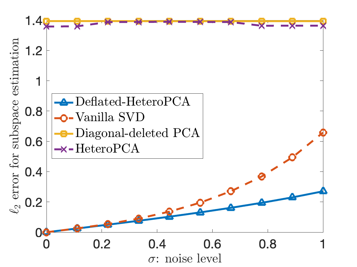
(a) $\kappa=5,n_{2}=1,000$, $\ell_{2}$ error

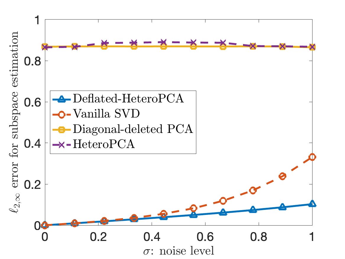
(b) $\kappa=5,n_{2}=1,000$, $\ell_{2,\infty}$ error

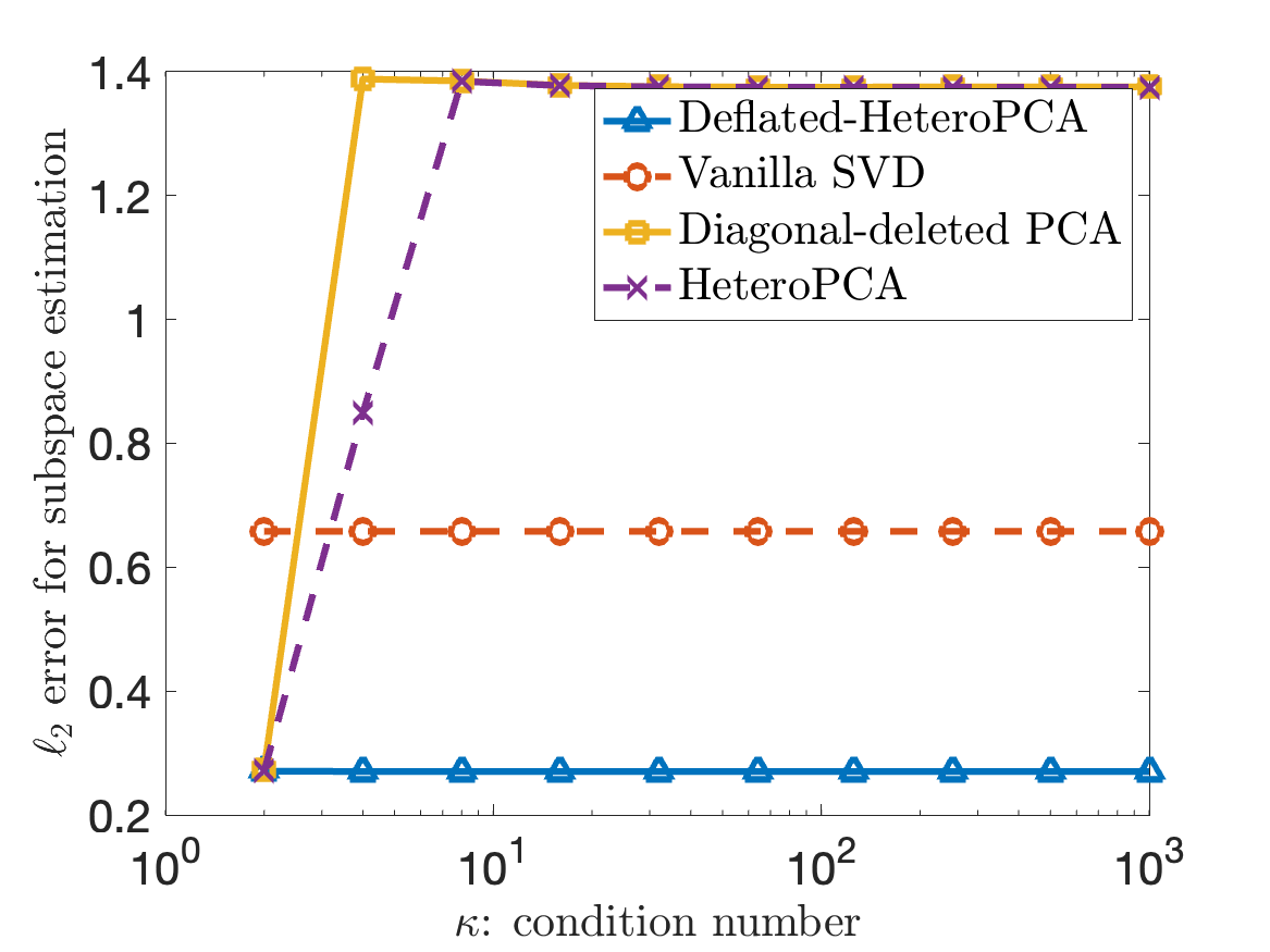
(c) $\omega=1,n_{2}=1,000$, $\ell_{2}$ error

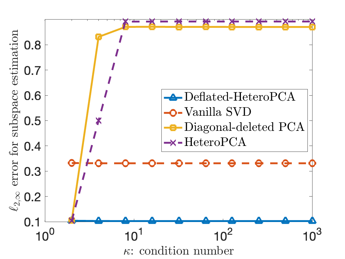
(d) $\omega=1,n_{2}=1,000$, $\ell_{2,\infty}$ error

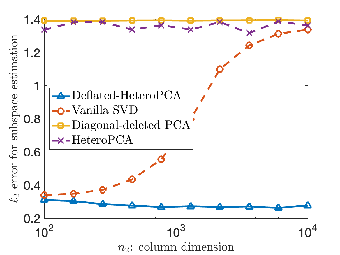
(e) $\omega=1,\kappa=5$, $\ell_{2}$ error

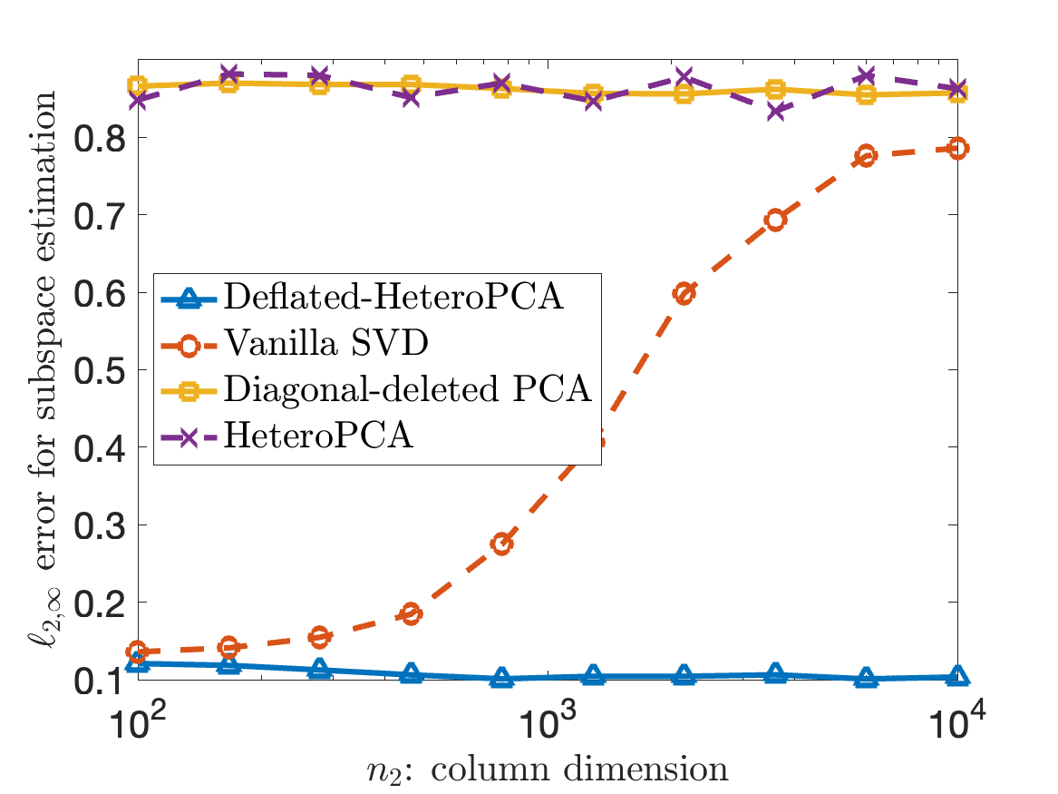
(f) $\omega=1,\kappa=5$, $\ell_{2,\infty}$ error

Figure 2: Estimation errors of $\bm{U}$ for Deflated-HeteroPCA, Diagonal-deleted PCA, HeteroPCA and Vanilla SVD for $r=3$. Plot (a) (resp. (b)) reports the $\ell_{2}$ (resp. $\ell_{2,\infty}$) error vs. the noise level $\omega$ (where $n_{1}=100,n_{2}=1,000,\kappa=5$). Plot (c) (resp. (d)) shows the $\ell_{2}$ (resp. $\ell_{2,\infty}$) error vs. the column dimension $\kappa$ (where $n_{1}=100,n_{2}=1,000,\omega=1$). Plot (e) (resp. (f)) displays the $\ell_{2}$ (resp. $\ell_{2,\infty}$) error vs. the condition number $n_{2}$ (where $n_{1}=100,\kappa=5,\omega=1$).

Low-rank subspace estimation from noisy observation.

To begin with, we consider the problem of estimating the column subspace of $\bm{X}^{\star}$ from the noisy data (3). We randomly generate $\bm{U}^{\star}\in\mathcal{O}^{n_{1},r}$ and $\bm{V}^{\star}\in\mathcal{O}^{n_{2},r}$, and $\bm{X}^{\star}=\bm{U}^{\star}\bm{\Sigma}^{\star}\bm{V}^{\star\top}$, where $\bm{\Sigma}^{\star}={\sf diag}(\sigma_{1}^{\star},\dots,\sigma_{r}^{\star})$. For each $i\in[n_{1}]$, we independently and uniformly draw $\omega_{i}\in[0,\omega]$, whereas the $E_{i,j}$’s are independently drawn from $\mathcal{N}(0,\omega_{i}^{2})$. We fix $n_{1}=100$, set $\sigma_{r}^{\star}=(n_{1}n_{2})^{1/4}+n_{1}^{1/2}$, and consider the following two settings: (i) $r=3$, $\sigma_{1}^{\star}=\kappa\sigma_{3}^{\star}$ and $\sigma_{2}^{\star}=\sigma_{3}^{\star}$; (ii) $r=5$, $\sigma_{1}^{\star}=\kappa\sigma_{5}^{\star}$, $\sigma_{2}^{\star}=\sigma_{3}^{\star}=\kappa^{1/2}\sigma_{5}^{\star}$ and $\sigma_{4}^{\star}=\sigma_{5}^{\star}$. We report the spectral-norm-based error$\|\bm{U}\bm{R}_{\bm{U}}-\bm{U}^{\star}\|$ and the $\ell_{2,\infty}$ error $\|\bm{U}\bm{R}_{\bm{U}}-\bm{U}^{\star}\|_{2,\infty}$ for each of the following four algorithms: (a) Deflated-HeteroPCA in Algorithm 2, where the numbers of iterations are chosen to be $t_{i}=10$; (b) the diagonal-deleted PCA procedure as in (10); (c) HeteroPCA in Algorithm 1, where the number of iterations is taken to be 100; (d) the vanilla SVD-based approach described in (8). The results for $r=3$ and $r=5$ are reported in Figures 2 and 3, respectively. As can be seen from the plots, the proposed Deflated-HeteroPCA algorithm significantly outperforms the other three methods, and it is the only algorithm whose performance is unaffected by the condition number $\kappa$.

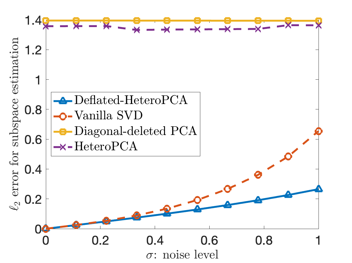
(a) $\kappa=5,n_{2}=1,000$, $\ell_{2}$ error

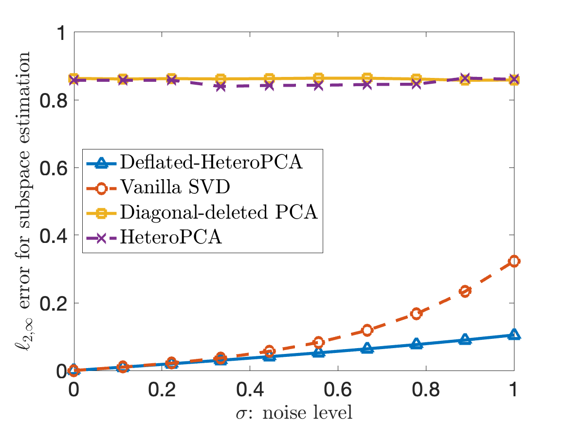
(b) $\kappa=5,n_{2}=1,000$, $\ell_{2,\infty}$ error

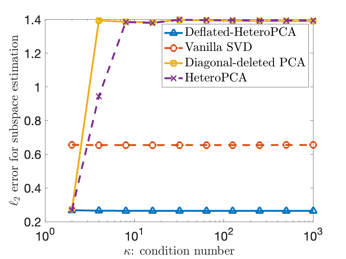
(c) $\omega=1,n_{2}=1,000$, $\ell_{2}$ error

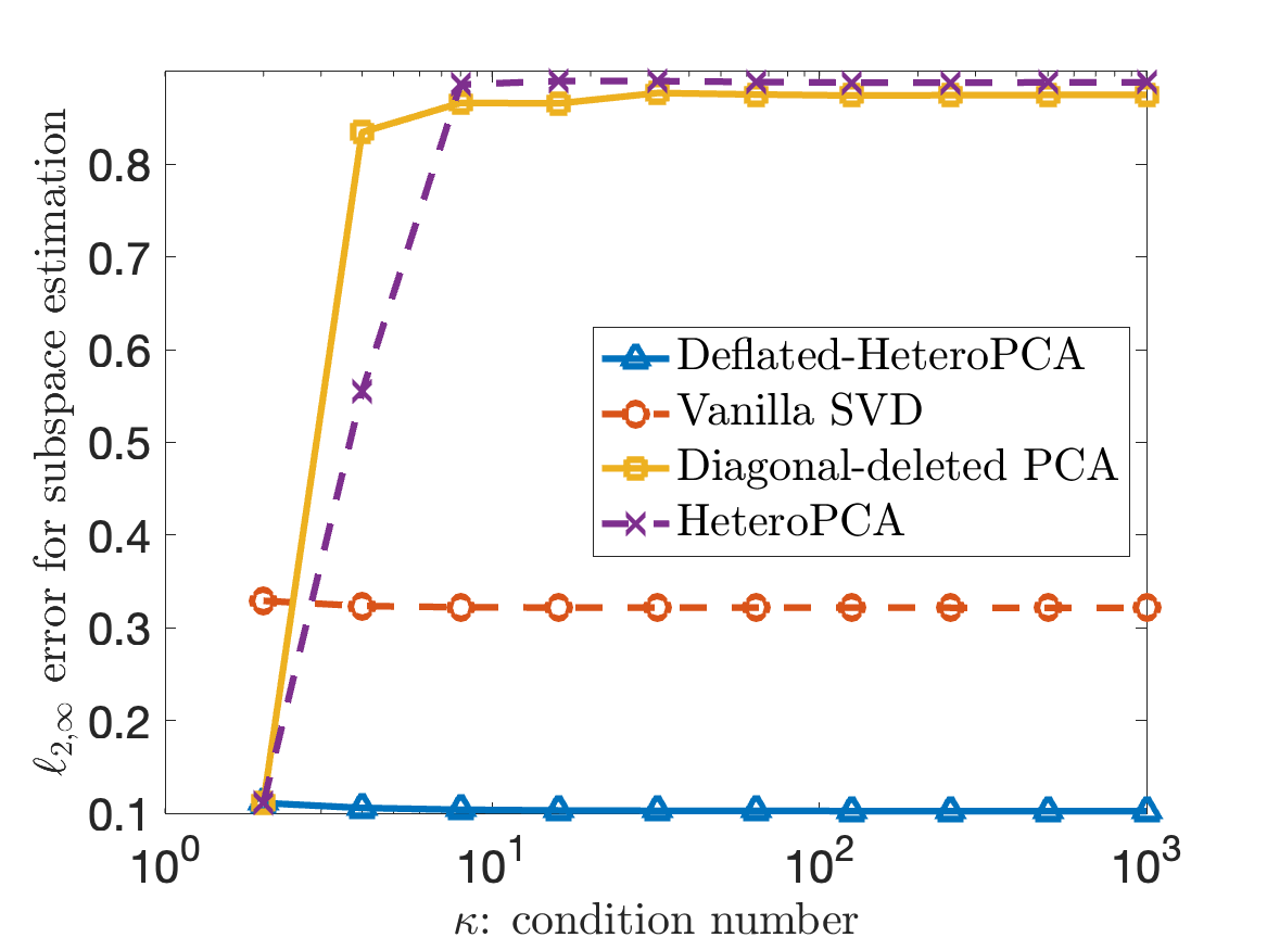
(d) $\omega=1,n_{2}=1,000$, $\ell_{2,\infty}$ error

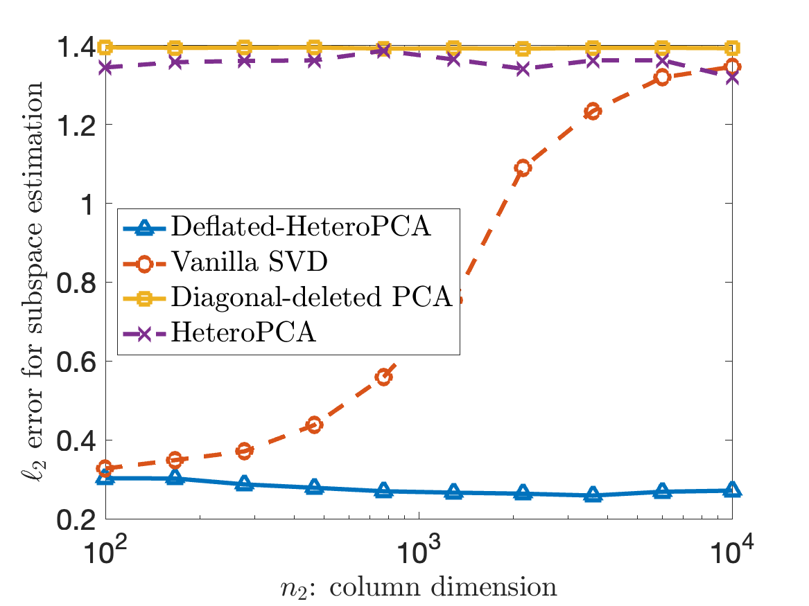
(e) $\omega=1,\kappa=5$, $\ell_{2}$ error

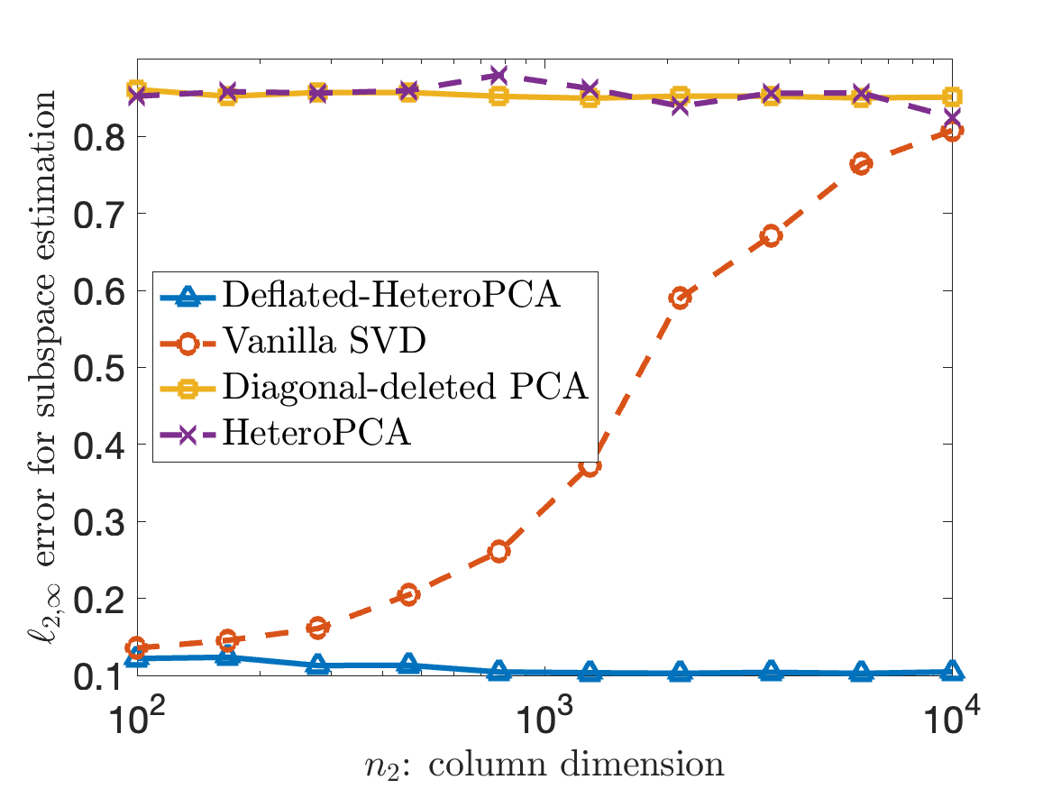
(f) $\omega=1,\kappa=5$, $\ell_{2,\infty}$ error

Figure 3: Estimation errors of $\bm{U}$ for Deflated-HeteroPCA, Diagonal-deleted PCA, HeteroPCA and Vanilla SVD when $r=5$. Plot (a) (resp. (b)) displays the $\ell_{2}$ (resp. $\ell_{2,\infty}$) error vs. the noise level $\omega$ (where $n_{1}=100,n_{2}=1,000,\kappa=5$). Plot (c) (resp. (d)) shows the $\ell_{2}$ (resp. $\ell_{2,\infty}$) error vs. the condition number $\kappa$ (where $n_{1}=100,n_{2}=1,000,\omega=1$). Plot (e) (resp. (f)) diaplsys the $\ell_{2}$ (resp. $\ell_{2,\infty}$) error vs. the column dimension $n_{2}$ (where $n_{1}=100,\kappa=5,\omega=1$).

Factor model.

We then turn attention to the factor model (32). We consider the case with $d=100,r=3$, and randomly generate the subspace $\bm{U}^{\star}\in\mathcal{O}^{d,3}$ and $\bm{F}=[\bm{f}_{1}\ \dots\ \bm{f}_{n}]\in\mathbb{R}^{3\times n}$ with i.i.d. standard Gaussian entries. We set the diagonal matrix $\bm{\Lambda}^{\star}={\sf diag}(\lambda_{1}^{\star},\lambda_{2}^{\star},\lambda_{3}^{\star})$ with $\lambda_{1}^{\star}=\kappa\lambda_{3}^{\star}$ and $\lambda_{2}^{\star}=\lambda_{3}^{\star}=(d/n)^{1/2}+d/n$. The noise matrix is generated in the same way as in the previous setting. We report in Figure 4 the $\ell_{2}$ and $\ell_{2,\infty}$ errors for the principal subspace for the four methods, Deflated-HeteroPCA, Diagonal-deleted PCA, HeteroPCA and Vanilla SVD. The numerical results suggest that the proposed Deflated-HeteroPCA algorithm achieves the best performance among all these methods, which is not affected as $\kappa_{\sf pc}$ varies.

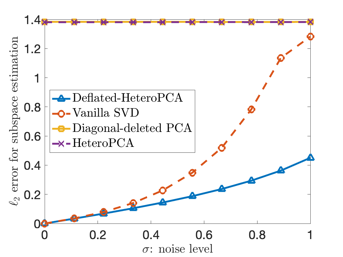
(a) $\kappa_{\sf pc}=100,n=1,000$, $\ell_{2}$ error

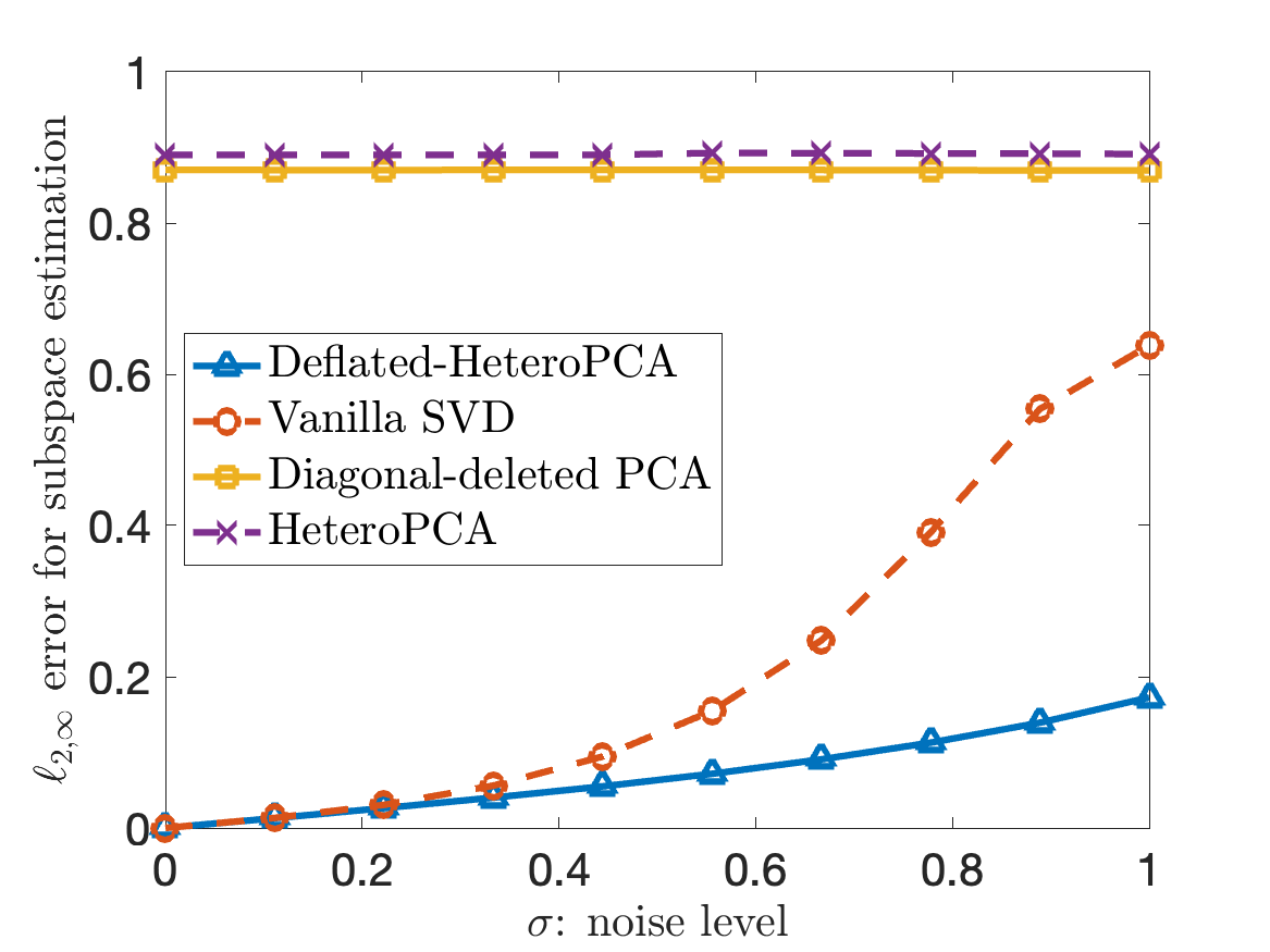
(b) $\kappa_{\sf pc}=100,n=1,000$, $\ell_{2,\infty}$ error

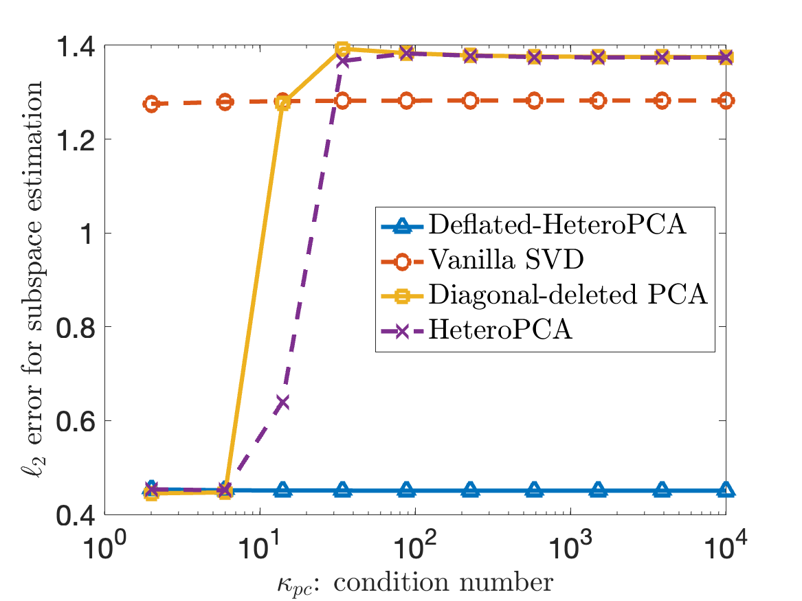
(c) $\omega=1,n=1,000$, $\ell_{2}$ error

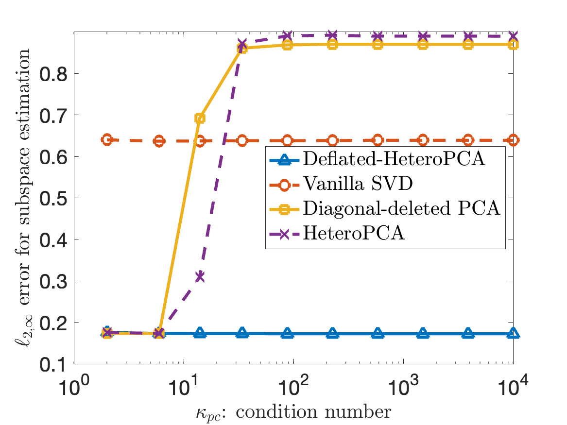
(d) $\omega=1,n=1,000$, $\ell_{2,\infty}$ error

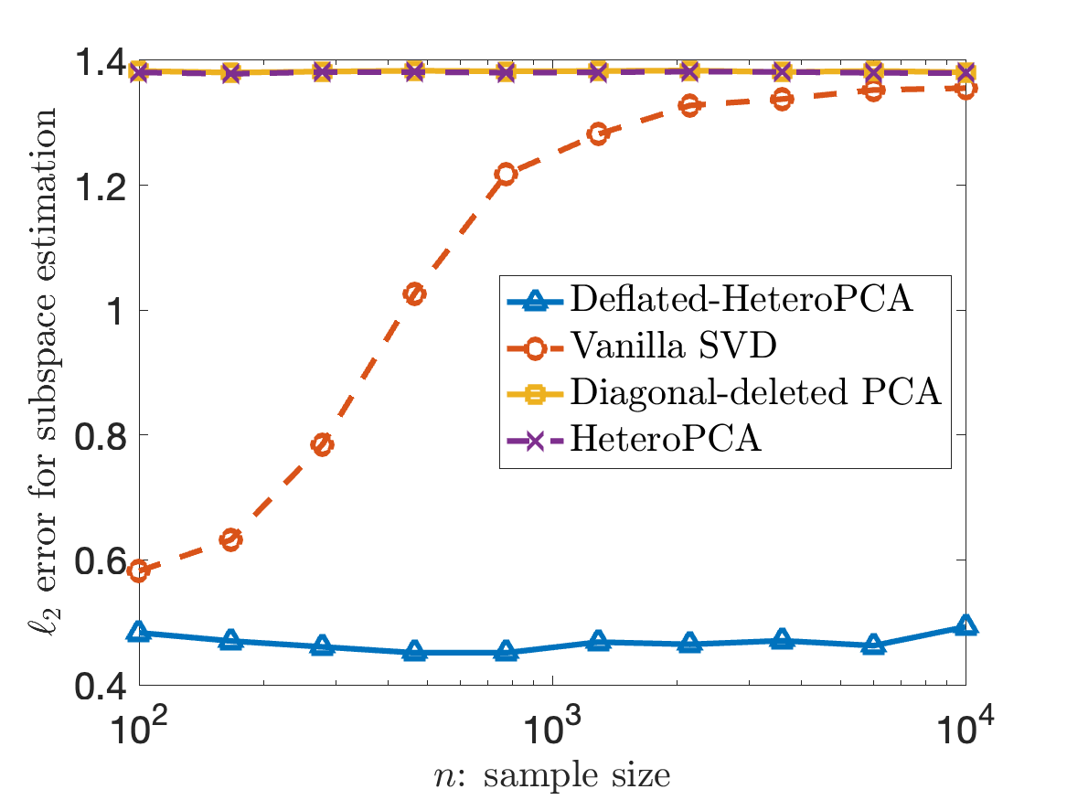
(e) $\omega=1,\kappa_{\sf pc}=100$, $\ell_{2}$ error

(f) $\omega=1,\kappa_{\sf pc}=100$, $\ell_{2,\infty}$ error

Figure 4: Estimation errors of $\bm{U}$ for Deflated-HeteroPCA, Diagonal-deleted PCA, HeteroPCA and Vanilla SVD under the factor model (32) when $r=3$. Plot (a) (resp. (b)) displays the $\ell_{2}$ (resp. $\ell_{2,\infty}$) error vs. the noise level $\omega$ (where $d=100,n=1,000,\kappa_{\sf pc}=100$). Plot (c) (resp. (d)) shows the $\ell_{2}$ (resp. $\ell_{2,\infty}$) error vs. the condition number $\kappa_{\sf pc}$ (where $d=100,n=1,000,\omega=1$). Plot (e) (resp. (f)) displays the $\ell_{2}$ (resp. $\ell_{2,\infty}$) error vs. the sample size $n$ (where $d=100,\kappa_{\sf pc}=100,\omega=1$).

Tensor PCA.

Finally, we conduct numerical experiments for the tensor PCA model (37). We fix $n=50$ and $r=3$, and introduce a quantity $\sigma^{\star}=n^{3/4}$. The subspaces $\bm{U}_{1}^{\star}\in\mathcal{O}^{100,3}$, $\bm{U}_{2}^{\star}\in\mathcal{O}^{100,3}$ and $\bm{U}_{3}^{\star}\in\mathcal{O}^{100,3}$ are generated randomly, and the core tensor $\mathcal{S}^{\star}\in\mathbb{R}^{3\times 3}$ is a diagonal tensor with entries $S_{1,1,1}=\kappa\sigma^{\star}$ and $S_{2,2,2}=S_{3,3,3}=\sigma^{\star}$. The noise tensor is generated in the following way: we first generate three random vectors $\bm{\alpha},\bm{\beta}$ and $\bm{\gamma}$, where $\{\alpha_{i}\}$, $\{\beta_{j}\}$, $\{\gamma_{k}\}$ are independently drawn from $[0,1]$. We then generate each $E_{i,j,k}$ independently from $\mathcal{N}(0,\omega^{2}\alpha_{i}^{2}\beta_{j}^{2}\gamma_{k}^{2})$. The above four subspace estimation methods are applied to obtain initial subspace estimates, followed by 50 iterations of HOOI to refine the subspace estimators and construct the final tensor estimates. Figures 5 and 6 report the initial subspace estimation errors and the final subspace/tensor estimation errors, respectively. We can see from these plots that the Deflated-HeteroPCA algorithm produces faithful initial estimators in terms of both the $\ell_{2}$ and $\ell_{2,\infty}$ errors, outperforming the other three methods. Moreover, compared with the other three methods, the Deflated-HeteroPCA algorithm serves as a more effective initialization scheme that can help one achieve more reliable subspace and tensor estimators.

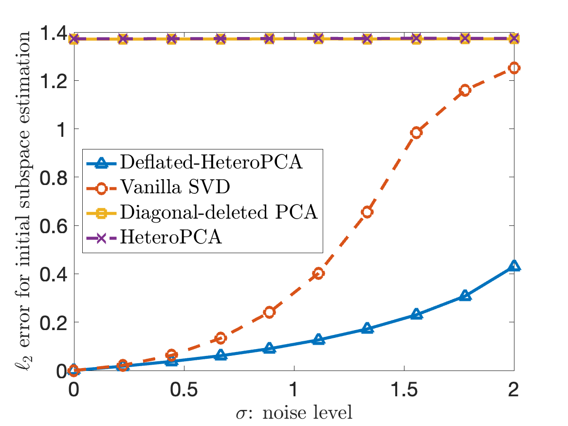
(a) $\kappa=6$, $\ell_{2}$ error

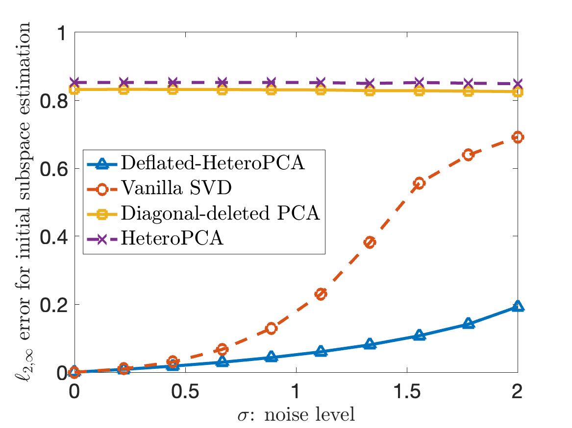
(b) $\kappa=6$, $\ell_{2,\infty}$ error

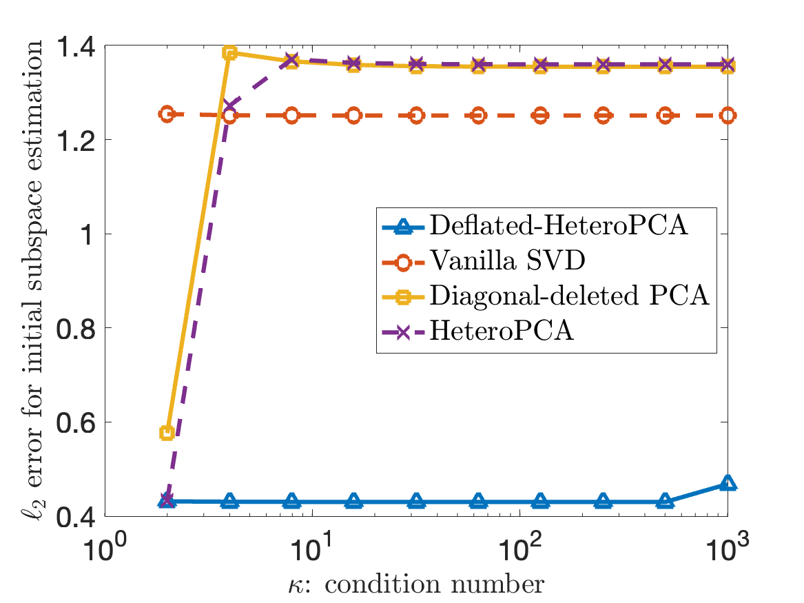
(c) $\omega=2$, $\ell_{2}$ error

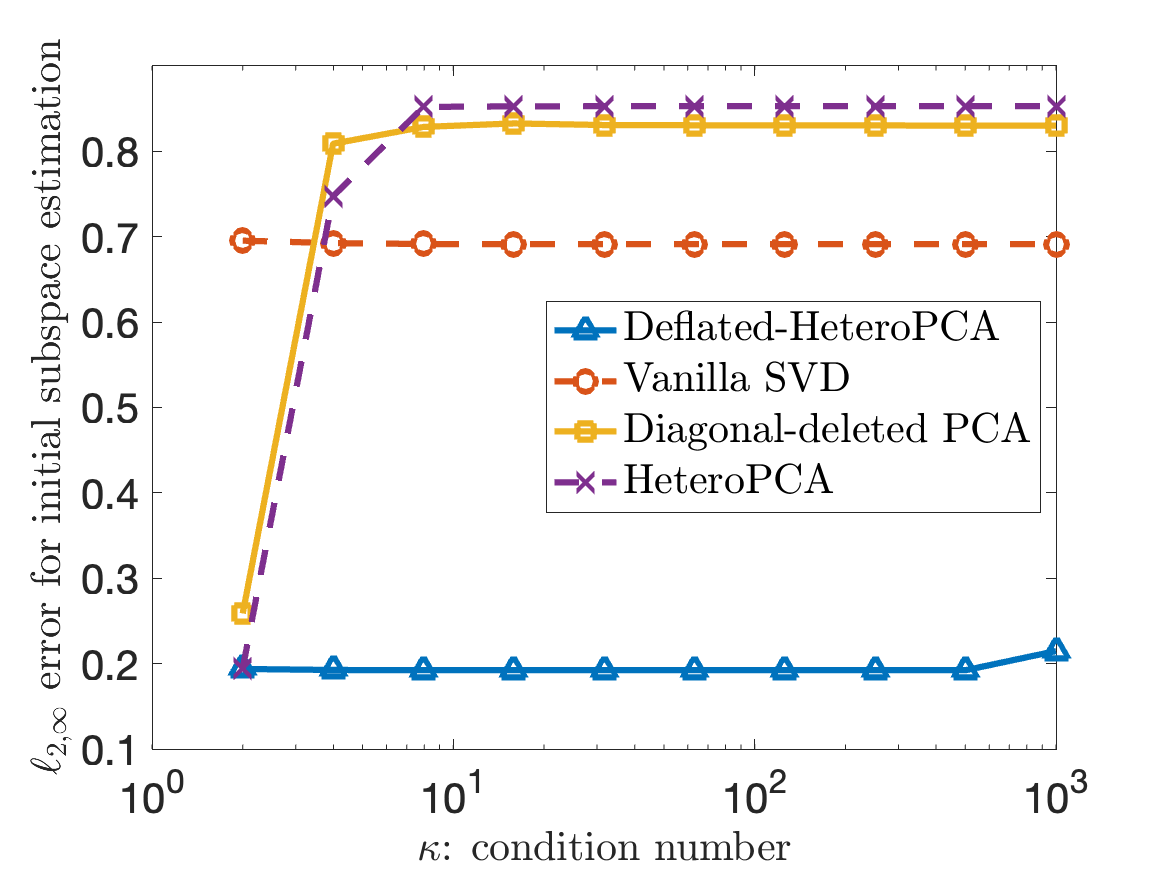
(d) $\omega=2$, $\ell_{2,\infty}$ error

Figure 5: Initial estimation errors of $\widehat{\bm{U}}_{1}^{0}$ for Deflated-HeteroPCA, Diagonal-deleted PCA, HeteroPCA and Vanilla SVD under the tensor SVD model (32). Plot (a) (resp. (b)) diplays the $\ell_{2}$ (resp. $\ell_{2,\infty}$) error vs. the noise level $\omega$ (where $n_{1}=n_{2}=n_{3}=50,r=3,\kappa=6$). Plot (c) (resp. (d)) shows the $\ell_{2}$ (resp. $\ell_{2,\infty}$) error vs. the condition number $\kappa$ (where $n_{1}=n_{2}=n_{3}=50,r=3,\omega=2$).

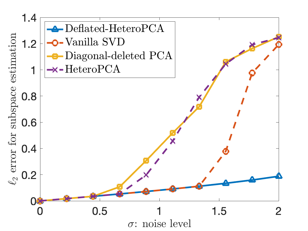
(a) $\kappa=6$, subspace estimation

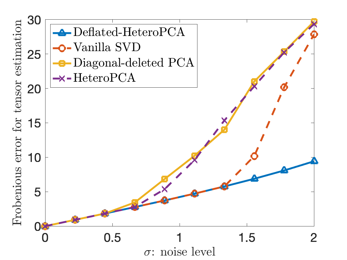
(b) $\kappa=6$, tensor estimation

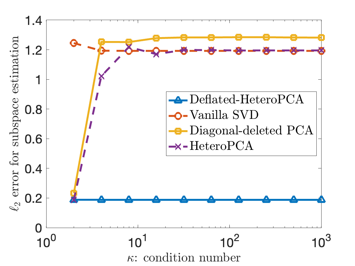
(c) $\omega=2$, subspace estimation

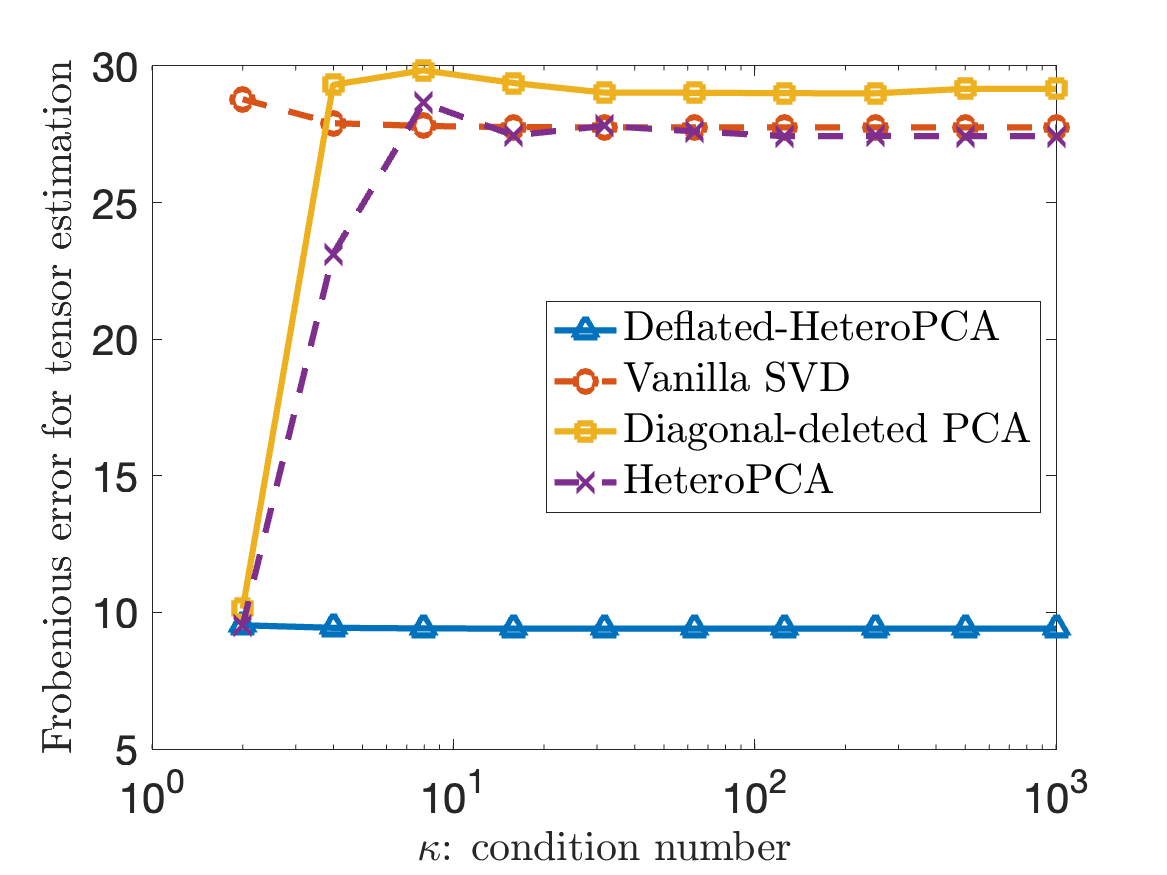
(d) $\omega=2$, tensor estimation

Figure 6: Final estimation errors of $\widehat{\bm{U}}_{1}$ and $\widehat{\bm{\mathcal{X}}}$ for Deflated-HeteroPCA, Diagonal-deleted PCA, HeteroPCA and Vanilla SVD under the tensor SVD model (32). We report (a) (resp. (b)) $\ell_{2}$ (resp. Frobenious) error of $\widehat{\bm{U}}_{1}$ (resp. $\widehat{\bm{\mathcal{X}}}$) vs. noise level $\omega$ (where $n_{1}=n_{2}=n_{3}=50,r=3,\kappa=6$); (c) (resp. (d)) $\ell_{2}$ (resp. Frobenious) error of $\widehat{\bm{U}}_{1}$ (resp. $\widehat{\bm{\mathcal{X}}}$) vs. condition number $\kappa$ (where $n_{1}=n_{2}=n_{3}=50,r=3,\omega=2$).

7 Related works

This paper is closely related to the problem of matrix denoising, which aims to estimate either a low-rank matrix or its column subspace based on noisy observations and spans a diverse array of applications (Chen et al., 2021b, ). In addition to the examples of factor models and tensor estimation (Cai and Zhang,, 2018; Cai et al.,, 2021; Zhu et al.,, 2019; Richard and Montanari,, 2014; Zhang and Xia,, 2018; Cai et al.,, 2021), it can also help us understand and solve several clustering problems (Rohe et al.,, 2011; Florescu and Perkins,, 2016; Cai et al.,, 2021; Chen et al.,, 2022; Cai and Zhang,, 2018; Löffler et al.,, 2021; Ndaoud,, 2022; Srivastava et al.,, 2022; Han et al., 2022a, ; Zhang and Zhou,, 2022). When it comes to the task of estimating the whole matrix, a number of methods have been put forward and thoroughly studied in the literature, including but not limited to singular value hard thresholding (Gavish and Donoho,, 2014; Chatterjee,, 2015), singular value soft thresholding (Cai et al.,, 2010; Koltchinskii et al.,, 2011; Donoho and Gavish,, 2014) and singular value shrinkage (Nadakuditi,, 2014; Gavish and Donoho,, 2017). Turning to the task of subspace estimation, the vanilla SVD-based approach (see (8)) has been commonly used and widely studied in the literature (Koltchinskii and Xia,, 2016; Cai and Zhang,, 2018; Bao et al.,, 2021; Xia,, 2021; Chen et al., 2021b, ). How to perform uncertainty quantification for this approach has also been demonstrated in the previous work (see (Chen et al., 2021b, )). In the scenario where the matrix dimensions are extremely unbalanced and the noise is heteroskedastic, however, such estimators can be highly suboptimal for subspace estimation. As already mentioned previously, the diagonal-deleted PCA and HeteroPCA algorithms have been proposed to improve the performance over the vanilla SVD approach (Cai et al.,, 2021; Zhang et al.,, 2022; Agterberg et al.,, 2022; Yan et al.,, 2021). In fact, it has also been shown in Yan et al., (2021) that the HeteroPCA admits a non-asymptotic distributional theory, which paves the way to construction of fine-grained confidence regions for this problem. Another family of effective algorithms — which can even accommodate the case when there is additional prior structure on the low-rank factors — is approximate message passing (Montanari and Venkataramanan,, 2021; Deshpande et al.,, 2017; Feng et al.,, 2022; Li et al.,, 2023; Li and Wei,, 2022; Montanari and Wu,, 2022), for which the existing theory often requires more stringent assumptions on the noise components (e.g., i.i.d. Gaussian). It is also worth mentioning that how to accelerate optimization-based low-rank estimation algorithms in spite of ill conditioning has been an active research topic as well, which oftentimes involves proper preconditioning (Tong et al.,, 2021; Xu et al.,, 2023); the statistical guarantees therein, however, are still dependent on the condition number.

With regards to the factor model, one can easily find numerous works on this topic. The model (32) has been extensively studied under the names of spiked covariance models (Johnstone,, 2001; Paul,, 2007; Bai and Ding,, 2012; Wang and Fan,, 2017; Donoho et al.,, 2018; Perry et al.,, 2018; Bao et al.,, 2022) and factor models (Lawley and Maxwell,, 1962; Bai and Li,, 2012; Fan et al.,, 2016; Bai and Wang,, 2016). Focusing on principal component estimation under heteroskedastic noise, Hong et al., (2016); Hong et al., 2018a ; Hong et al., 2018b investigate the case where the noise components within each noise vector $\bm{\varepsilon}_{j}$ are i.i.d., and develop asymptotic analysis for PCA and a variant called Weighted PCA. Turning to non-asymptotic analysis, the theoretical performances of diagonal-deleted PCA (Cai et al.,, 2021) and HeteroPCA have been investigated in (Cai et al.,, 2021; Zhang et al.,, 2022; Yan et al.,, 2021). It is also worth noting that principal component estimation in the presence of missing data encounters additional challenges (Cai et al.,, 2021; Zhang et al.,, 2022; Zhu et al.,, 2019; Pavez and Ortega,, 2020; Yan et al.,, 2021), which is beyond the scope of this work.

Another important example considered in this paper is the tensor PCA or tensor SVD model (37). Under this model, Richard and Montanari, (2014); Hopkins et al., (2015); Anandkumar et al., (2017); Arous et al., (2019); Perry et al., (2020) study the statistical and computational limits for rank-$1$ tensors. For low Tucker-rank tensors, many methods have been proposed for tensor/subspace estimation, including high-order SVD (HOSVD, De Lathauwer et al., 2000a ), high-order orthogonal iteration (HOOI, De Lathauwer et al., 2000b ; Zhang and Xia, (2018)), the sequentially truncated higher-order singular value decomposition algorithm (ST-HOSVD, Vannieuwenhoven et al., (2012)), projected gradient descent (Han et al., 2022b, ), and scaled gradient descent (Tong et al.,, 2022). When the noise tensor has i.i.d. Gaussian entries, Zhang and Xia, (2018) proves the statistical and computational limit for the tensor SVD and reveals that the HOOI achieves the optimal performance both statistically and computationally. Allowing the noise to be heteroskedastic, Han et al., 2022b shows that the optimal error rate can be achieved by the projected gradient descent with the initialization given by the HeteroPCA if the condition number of the true tensor is bounded. In contrast to the prior literature, we consider the tensor and subspace estimation problem under heteroskedastic noise and aim to accommodate an arbitrarily large condition number; we show that the HOOI algorithm initialized by Deflated-HeteroPCA yields optimal theoretical guarantees. In addition to the Tucker-rank decomposition, the tensor PCA/SVD model with the low CP-rank structure (Kolda and Bader,, 2009; Anandkumar et al.,, 2014; Cai et al.,, 2021; Cai et al., 2022a, ; Cai et al.,, 2023) and the low tensor-train-rank structure (Zhou et al.,, 2022; Cai et al., 2022b, ) have also received much attention in the past few years.

In addition, recent years have witnessed much acitivity in developing $\ell_{\infty}$ and $\ell_{2,\infty}$ theoretical guarantees for singular subspaces and eigenspaces (Zhong and Boumal,, 2018; Fan et al.,, 2018; Cape et al.,, 2019; Agterberg et al.,, 2022). Particularly worth noting is the leave-one-out analysis framework, which emerges as a powerful tool to derive fine-grained (e.g., entrywise or rowwise) bounds and finds applications in numerous high-dimensional estimation problems (Zhong and Boumal,, 2018; Ma et al.,, 2020; Chen et al., 2019a, ; Abbe et al.,, 2020; Chen et al.,, 2020; Chen et al., 2019b, ; Chen et al., 2021c, ; Cai et al.,, 2021; Chen et al., 2021d, ; Cai et al., 2022a, ; Abbe et al.,, 2022; Yan et al.,, 2021; Ling,, 2022; Zhang and Zhou,, 2022; Yang and Ma,, 2022). However, existing $\ell_{2,\infty}$ estimation guaranteed obtained by means of the leave-one-out technique still rely on the condition number. To achieve a condition-number-free $\ell_{2,\infty}$ bound, we provide a novel analysis based on the representation theorem presented in Xia, (2021). The idea also shares similar spirit with the Neumann trick, which is commonly used in $\ell_{\infty}$ eigenvector analysis (Eldridge et al.,, 2018; Chen et al., 2021a, ; Cheng et al.,, 2021).

8 Discussion

This paper has studied subspace estimation from noisy low-rank matrices in the presence of unbalanced dimensionality and heteroskedastic noise. Recognizing a curse of ill-conditioning that appears in two cutting-edge algorithms, we have developed a new algorithm called Deflated-HeteroPCA to strengthen the state-of-the-art statistical performance in the face of a large condition number, without compromising the range of SNRs that can be accommodated. We have demonstrated that the proposed estimator enjoys nearly rate-optimal statistical guarantees (in terms of both the spectral-norm error and the more fine-grained $\ell_{2,\infty}$-based error), which are unaffected by the underlying condition number (regardless of how large it is). When applied to two concrete statistical models (i.e., factor models and tensor PCA), our theory has led to remarkable improvement over the prior art (particularly for the ill-conditioned scenarios).

Our work suggests several potential avenues for future investigation. For example, the signal-to-noise ratio conditions (15a) and (20a) in our theory remain sub-optimal when it comes to their dependency on the rank $r$. How to tighten this rank dependency calls for a more refined analysis or a more powerful algorithm. Another direction worthy of future studies is the case with missing data (i.e., suppose we only have access to highly incomplete observations of the entries of the data matrix $\bm{Y}$ in (1)). It would be of great interest to extend our approach and develop a computationally efficient estimator that enjoys condition-number-free and rate-optimal estimation guarantees in the presence of missing data.

Appendix A Proof of Theorem 1 ($\ell_{2}$ analysis for Deflated-HeteroPCA)

Before continuing, we introduce some notation about some intermediate objects that appear in our algorithm, which will be useful in the proofs. First, set

$$\bm{G}_{k+1}^{0}:=\bm{G}_{k},\qquad 0\leq k\leq k_{\sf max},$$ (43a)

where we recall that

$$\bm{G}_{0}=\mathcal{P}_{\sf off\text{-}diag}(\bm{Y}\bm{Y}^{\top}).$$

For each $$t=0,1,\dots,t_{k+1} k=0,1,\dots,k_{\sf max}$$ and , let

$$\bm{U}_{k+1}^{t}\bm{\Lambda}_{k+1}^{t}\bm{U}_{k+1}^{t\top}:=\text{ the rank-}r_{k}\text{ leading eigendecompostion of }\bm{G}_{k+1}^{t},$$ (43b)

and define

$$\bm{G}_{k+1}^{t+1}:=\mathcal{P}_{\sf off\text{-}diag}\left(\bm{G}_{k+1}^{t}\right)+\mathcal{P}_{\sf diag}\left(\bm{U}_{k+1}^{t}\bm{\Lambda}_{k+1}^{t}\bm{U}_{k+1}^{t\top}\right),$$ (43c)

which corresponds to the matrix computed by HeteroPCA in the $t$-th iteration of the $(k+1)$-th round.

In this section, we intend to prove a slightly more general version of Theorem 1 as follows.

Theorem 3.

Suppose that Assumption 1 holds. Suppose that

$$\sigma_{r}^{\star} \geq C_{0}r\sqrt{\mu r\omega_{\sf max}^{2}+\omega_{\sf col}\left(\omega_{\sf row}+\omega_{\sf col}\right)}\sqrt{\log n}$$ (44a)

$$\mu \leq c_{0}\frac{n_{1}}{r^{3}}$$ (44b)

for some sufficiently large (resp. small) constant $C_{0}>0$ (resp. $c_{0}>0$). If the numbers of iterations obey (16a), then with probability exceeding $1-O(n^{-10})$, the output returned by Algorithm 2 satisfies

$$\left\|\bm{U}\bm{R}_{\bm{U}}-\bm{U}^{\star}\right\|\lesssim\frac{\sqrt{\left(\mu r\omega_{\sf max}^{2}+\omega_{\sf col}^{2}\right)\log n}}{\sigma_{r}^{\star}}+\frac{\omega_{\sf col}\omega_{\sf row}\log n}{\sigma_{r}^{\star 2}}+e^{-t_{k_{\sf max}}}.$$ (45)

Evidently, if we further have $0<\mu r\omega_{{\sf max}}^{2}\lesssim\omega_{\sf col}^{2}$ and if the number of iterations $t_{k_{\sf max}}$ obeys (16b), then it is easy to check that the bound (45) (resp. the signal-to-noise ratio condition (44a)) implies (17) (resp. (15a)). This allows us to focus attention on establishing Theorem 3.

A.1 A key intermediate result and the proof of Theorem 3

Towards proving Theorem 3, we first single out a deterministic result that plays a crucial role in bounding $\left\|\bm{U}\bm{R}_{\bm{U}}-\bm{U}^{\star}\right\|$; its proof is postponed to Section A.2.

Theorem 4.

Suppose that we observe a matrix $\bm{M}=\overline{\bm{U}}\,\overline{\bm{\Lambda}}\,\overline{\bm{U}}^{\top}+\bm{Z}$, where $\overline{\bm{\Lambda}}\in\mathbb{R}^{r\times r}$ is a diagonal matrix with diagonal entries $\overline{\lambda}_{1}\geq\dots\geq\overline{\lambda}_{r}>0$ and $\overline{\bm{U}}\in\mathcal{O}^{n_{1},r}$ satisfies

$$\|\overline{\bm{U}}\|_{2,\infty}\leq\sqrt{\frac{\overline{\mu}r}{n_{1}}}\qquad\text{with }~{}\overline{\mu}\leq c_{0}\frac{n_{1}}{r^{3}}$$ (46a)

for some sufficiently small constant $$c_{0}>0$$. Also, assume that

$$\overline{\lambda}_{r} \geq C_{0}r\|\mathcal{P}_{\sf off\text{-}diag}(\bm{Z})\|.$$ (46b)

Then Algorithm 2 with initialization $\bm{G}_{0}=\mathcal{P}_{\sf off\text{-}diag}(\bm{M})$ yields an estimate $\bm{U}$ satisfying

$$\big{\|}\bm{U}\bm{U}^{\top}-\overline{\bm{U}}\,\overline{\bm{U}}^{\top}\big{\|}\lesssim\frac{\left\|\mathcal{P}_{\sf off\text{-}diag}\left(\bm{Z}\right)\right\|}{\overline{\lambda}_{r}}+e^{-t_{k_{\sf max}}},$$ (47)

provided that the numbers of iterations obey

$$t_{1} >\log\left(\frac{\frac{\overline{\mu}r}{n_{1}}\overline{\lambda}_{1}}{\sqrt{\frac{\overline{\mu}r}{n_{1}}}\overline{\lambda}_{r_{1}+1}+\left\|\mathcal{P}_{\sf off\text{-}diag}\left(\bm{Z}\right)\right\|}\right)\,\vee 0$$ (48a)

$$t_{k} >\log\left(\frac{7\sqrt{\frac{\overline{\mu}r}{n_{1}}}\overline{\lambda}_{r_{k-1}+1}+\left\|\mathcal{P}_{\sf off\text{-}diag}\left(\bm{Z}\right)\right\|}{\sqrt{\frac{\overline{\mu}r}{n_{1}}}\overline{\lambda}_{r_{k}+1}+\left\|\mathcal{P}_{\sf off\text{-}diag}\left(\bm{Z}\right)\right\|}\right),\quad 1\leq k\leq k_{\sf max}-1.$$ (48b)

In a nutshell, Theorem 4 asserts that the subspace estimation error of Deflated-HeteroPCA depends only on (i) the size of $\bm{Z}$ after diagonal deletion and (ii) the $r$-th leading eigenvalue of $\overline{\bm{U}}\,\overline{\bm{\Lambda}}\,\overline{\bm{U}}^{\top}$, provided that the numbers of iterations exceed some logarithmic factors. Notably, the estimation error bound (47) holds irrespective of the condition number of $\overline{\bm{\Lambda}}$ and the noise entries $\mathcal{P}_{\sf diag}(\bm{Z})$ in the diagonal (in fact, these diagonal entries of $\bm{Z}$ are never used by Deflated-HeteroPCA).

We now demonstrate how to invoke Theorem 4 to establish Theorem 3, which consists of several steps below. Before proceeding, we isolate one important matrix $\bm{U}^{\star}\bm{\Sigma}^{\star}+\bm{E}\bm{V}^{\star}\in\mathbb{R}^{n_{1}\times r}$, and denote its SVD as

$$\widetilde{\bm{U}}\widetilde{\bm{\Sigma}}\widetilde{\bm{W}}^{\top}=\bm{U}^{\star}\bm{\Sigma}^{\star}+\bm{E}\bm{V}^{\star},$$ (49)

where $\widetilde{\bm{U}}\in\mathcal{O}^{n_{1},r},\widetilde{\bm{W}}\in\mathcal{O}^{r,r}$ and $\widetilde{\bm{\Sigma}}={\sf diag}(\widetilde{\sigma}_{1},\dots,\widetilde{\sigma}_{r})$ with $\widetilde{\sigma}_{1}\geq\dots\geq\widetilde{\sigma}_{r}\geq 0$.

Step 1: bounding the spectrum of $\widetilde{\bm{\Sigma}}^{-1}$.

We start by controlling the spectrum of $\widetilde{\bm{\Sigma}}$. Taking Weyl’s inequality, Assumption 1 and Lemma 5 together implies that with probability exceeding $1-O(n^{-10})$,

$$\max_{1\leq i\leq r}\left|\widetilde{\sigma}_{i}-\sigma_{i}^{\star}\right|\leq\left\|\bm{E}\bm{V}^{\star}\right\| \lesssim\sqrt{\left(r\omega_{\sf max}^{2}+\omega_{\sf col}^{2}\right)\log n}+B\log n\sqrt{\frac{\mu_{2}r}{n_{2}}}$$

$$\lesssim\sqrt{\left(r\omega_{\sf max}^{2}+\omega_{\sf col}^{2}\right)\log n}+\frac{\omega_{\sf row}}{\sqrt{\log n}}\log n\sqrt{\frac{\mu_{2}r}{n_{2}}}$$

$$\lesssim\sqrt{\left(r\omega_{\sf max}^{2}+\omega_{\sf col}^{2}\right)\log n}+\sqrt{n_{2}}\omega_{\sf max}\sqrt{\log n}\sqrt{\frac{\mu r}{n_{2}}}$$

$$\lesssim\sqrt{\left(\mu r\omega_{\sf max}^{2}+\omega_{\sf col}^{2}\right)\log n},$$ (50)

where the second line relies on Assumption 1. Consequently, one can deduce that

$$\big{\|}\widetilde{\bm{\Sigma}}^{-1}\big{\|}=\frac{1}{\widetilde{\sigma}_{r}}\leq\frac{1}{\sigma^{\star}_{r}-\left\|\bm{E}\bm{V}^{\star}\right\|}\leq\frac{\sqrt{2}}{\sigma^{\star}_{r}},$$ (51)

provided that $\sigma^{\star}_{r}\geq C_{0}\sqrt{\left(\mu r\omega_{\sf max}^{2}+\omega_{\sf col}^{2}\right)\log n}$ for some large enough constant $C_{0}>0$. It is also seen that

$$\sigma^{\star}_{r} \leq\widetilde{\sigma}_{r}+\left\|\bm{E}\bm{V}^{\star}\right\|\leq\widetilde{\sigma}_{r}+\frac{1}{2}\sigma^{\star}_{r}$$

$$\Longrightarrow\qquad\sigma^{\star}_{r}\leq 2\widetilde{\sigma}_{r}.$$ (52)

Repeating the same argument also reveals that

$$\frac{1}{2}\widetilde{\sigma}_{i}\leq\sigma^{\star}_{i}\leq 2\widetilde{\sigma}_{i},\qquad 1\leq i\leq r.$$ (53)

Step 2: bounding $\|\widetilde{\bm{U}}\|_{2,\infty}$.

We now move on to control $\|\widetilde{\bm{U}}\|_{2,\infty}$, a sort of incoherence condition needed in order to invoke Theorem 4 (see (46a)). Towards this, we would like to first the discrepancy between $\bm{U}^{\star}\bm{U}^{\star\top}\widetilde{\bm{U}}$ and $\widetilde{\bm{U}}$, which would in turn allow us to switch attention to the $\ell_{2,\infty}$ norm of $\bm{U}^{\star}\bm{U}^{\star\top}\widetilde{\bm{U}}$. Recognizing that

$$\big{(}\widetilde{\bm{U}}-\bm{U}^{\star}\bm{U}^{\star\top}\widetilde{\bm{U}}\big{)}\widetilde{\bm{\Sigma}}\widetilde{\bm{W}}^{\top} =\mathcal{P}_{\bm{U}_{\perp}^{\star}}\widetilde{\bm{U}}\widetilde{\bm{\Sigma}}\widetilde{\bm{W}}^{\top}=\mathcal{P}_{\bm{U}_{\perp}^{\star}}\left(\bm{U}^{\star}\bm{\Sigma}^{\star}+\bm{E}\bm{V}^{\star}\right)$$

$$=\bm{E}\bm{V}^{\star}-\bm{U}^{\star}\bm{U}^{\star\top}\bm{E}\bm{V}^{\star},$$ (54)

we can readily use $\|\widetilde{\bm{W}}\|=1$ to derive

$$\big{\|}\bm{U}^{\star}\bm{U}^{\star\top}\widetilde{\bm{U}}-\widetilde{\bm{U}}\big{\|}_{2,\infty} =\left\|\left(\bm{E}\bm{V}^{\star}-\bm{U}^{\star}\bm{U}^{\star\top}\bm{E}\bm{V}^{\star}\right)\widetilde{\bm{W}}\widetilde{\bm{\Sigma}}^{-1}\right\|_{2,\infty}$$

$$\leq\left(\left\|\bm{E}\bm{V}^{\star}\right\|_{2,\infty}+\left\|\bm{U}^{\star}\bm{U}^{\star\top}\bm{E}\bm{V}^{\star}\right\|_{2,\infty}\right)\big{\|}\widetilde{\bm{\Sigma}}^{-1}\big{\|}.$$ (55)

In view of Lemma 5 and Assumption 1, with probability exceeding $1-O(n^{-10})$, one has

$$\left\|\bm{E}\bm{V}^{\star}\right\|_{2,\infty}\lesssim\left(B\log n+\omega_{\sf row}\sqrt{\log n}\right)\sqrt{\frac{\mu_{2}r}{n_{2}}}\asymp\omega_{\sf row}\sqrt{\log n}\sqrt{\frac{\mu_{2}r}{n_{2}}}$$

and

$$\left\|\bm{U}^{\star}\bm{U}^{\star\top}\bm{E}\bm{V}^{\star}\right\|_{2,\infty} \leq\left\|\bm{U}^{\star}\right\|_{2,\infty}\left\|\bm{U}^{\star\top}\bm{E}\bm{V}^{\star}\right\|$$

$$\lesssim\sqrt{\frac{\mu_{1}r}{n_{1}}}\left(B\frac{\mu r}{\sqrt{n_{1}n_{2}}}\log n+\left(\sqrt{\frac{\mu r}{n_{2}}}\omega_{\sf row}+\sqrt{\frac{\mu r}{n_{1}}}\omega_{\sf col}\right)\sqrt{\log n}\right)$$

$$\lesssim\sqrt{\frac{\mu_{1}r}{n_{1}}}\left(\frac{\omega_{\sf row}}{\sqrt{\log n}}\sqrt{\frac{\mu r}{n_{2}}}\log n+\left(\sqrt{\frac{\mu r}{n_{2}}}\omega_{\sf row}+\sqrt{\frac{\mu r}{n_{1}}}\omega_{\sf col}\right)\sqrt{\log n}\right)$$

$$\lesssim\sqrt{\frac{\mu_{1}r}{n_{1}}}\left(\sqrt{\frac{\mu r}{n_{2}}}\omega_{\sf row}+\sqrt{\frac{\mu r}{n_{1}}}\omega_{\sf col}\right)\sqrt{\log n},$$

where the second line has also made use of the assumption that $\mu r\lesssim n_{1}$. Putting (A.1) and the previous two inequalities together and using the assumption $\mu r\lesssim n_{1}$, we arrive at

$$\big{\|}\bm{U}^{\star}\bm{U}^{\star\top}\widetilde{\bm{U}}-\widetilde{\bm{U}}\big{\|}_{2,\infty} \lesssim\left(\omega_{\sf row}\sqrt{\log n}\sqrt{\frac{\mu_{2}r}{n_{2}}}+\sqrt{\frac{\mu_{1}r}{n_{1}}}\left(\sqrt{\frac{\mu r}{n_{2}}}\omega_{\sf row}+\sqrt{\frac{\mu r}{n_{1}}}\omega_{\sf col}\right)\sqrt{\log n}\right)\frac{1}{\sigma^{\star}_{r}}$$

$$\lesssim\frac{\left(\sqrt{\frac{\mu r}{n_{2}}}\omega_{\sf row}+\frac{\mu r}{n_{1}}\omega_{\sf col}\right)\sqrt{\log n}}{\sigma_{r}^{\star}}$$

$$\ll\frac{1}{r}=\sqrt{\frac{\left(\frac{n_{1}}{r^{3}}\right)r}{n_{1}}}$$ (56)

with probability exceeding $1-O(n^{-10})$, provided that

$$\sigma_{r}^{\star}\gg r\left[\left(\sqrt{\frac{\mu r}{n_{2}}}\omega_{\sf row}+\frac{\mu r}{n_{1}}\omega_{\sf col}\right)\sqrt{\log n}+\sqrt{\left(\mu r\omega_{\sf max}^{2}+\omega_{\sf col}^{2}\right)\log n}\right]\asymp r\sqrt{\left(\mu r\omega_{\sf max}^{2}+\omega_{\sf col}^{2}\right)\log n}.$$

As a result, with probability at least $1-O(n^{-10})$, we reach the following upper bound:

$$\big{\|}\widetilde{\bm{U}}\big{\|}_{2,\infty} \leq\big{\|}\bm{U}^{\star}\bm{U}^{\star\top}\widetilde{\bm{U}}-\widetilde{\bm{U}}\big{\|}_{2,\infty}+\big{\|}\bm{U}^{\star}\bm{U}^{\star\top}\widetilde{\bm{U}}\big{\|}_{2,\infty}$$

$$\leq\big{\|}\bm{U}^{\star}\bm{U}^{\star\top}\widetilde{\bm{U}}-\widetilde{\bm{U}}\big{\|}_{2,\infty}+\left\|\bm{U}^{\star}\right\|_{2,\infty}\big{\|}\bm{U}^{\star\top}\widetilde{\bm{U}}\big{\|}$$

$$\leq\big{\|}\bm{U}^{\star}\bm{U}^{\star\top}\widetilde{\bm{U}}-\widetilde{\bm{U}}\big{\|}_{2,\infty}+\sqrt{\frac{\mu r}{n_{1}}}\ll\sqrt{\frac{\left(\frac{n_{1}}{r^{3}}\right)r}{n_{1}}},$$ (57)

where the last inequality holds under our assumption that $\mu r^{3}\lesssim n_{1}$. With this $\ell_{2,\infty}$ bound for $\widetilde{\bm{U}}$ in place — which reveals an upper bound $O\big{(}\frac{n_{1}}{r^{3}}\big{)}$ on the incoherence parameter of $\widetilde{\bm{U}}$ (see the requirement (46a)) — we can proceed to apply Theorem 4 in the next step.

Step 3: bounding $\|\bm{U}\bm{U}^{\top}-\bm{U}^{\star}\bm{U}^{\star\top}\|$ and $\|\bm{U}\bm{R}_{\bm{U}}-\bm{U}^{\star}\|$.

In this step, we shall first invoke Theorem 4 to control $\|\bm{U}\bm{U}^{\top}-\widetilde{\bm{U}}\widetilde{\bm{U}}^{\top}\|$, and then apply standard eigenspace perturbation theory to bound $\|\widetilde{\bm{U}}\widetilde{\bm{U}}^{\top}-\bm{U}^{\star}\bm{U}^{\star\top}\|$.

To begin with, let us write

$$\bm{Y}\bm{Y}^{\top}=\left(\bm{X}^{\star}+\bm{E}\right)\left(\bm{X}^{\star}+\bm{E}\right)^{\top} =\left(\bm{U}^{\star}\bm{\Sigma}^{\star}+\bm{E}\bm{V}^{\star}\right)\left(\bm{U}^{\star}\bm{\Sigma}^{\star}+\bm{E}\bm{V}^{\star}\right)^{\top}+\big{(}\bm{E}\bm{E}^{\top}-\bm{E}\bm{V}^{\star}\bm{V}^{\star\top}\bm{E}^{\top}\big{)}.$$ (58)

Recall that $\widetilde{\bm{U}}$ represents the column subspace of $\left(\bm{U}^{\star}\bm{\Sigma}^{\star}+\bm{E}\bm{V}^{\star}\right)\left(\bm{U}^{\star}\bm{\Sigma}^{\star}+\bm{E}\bm{V}^{\star}\right)^{\top}$ (cf. (49)). Thus, in order to apply Theorem 4 to control $\|\bm{U}\bm{U}^{\top}-\widetilde{\bm{U}}\widetilde{\bm{U}}^{\top}\|$, the key lies in coping with $\|\mathcal{P}_{\sf off\text{-}diag}(\bm{\bm{E}\bm{E}^{\top}-\bm{E}\bm{V}^{\star}\bm{V}^{\star\top}\bm{E}^{\top}})\|$. By virtue of Lemma 7 and Assumption 1, with probability exceeding $1-O(n^{-10})$ we have

$$\left\|\mathcal{P}_{\sf off\text{-}diag}\big{(}\bm{E}\bm{E}^{\top}\big{)}\right\| \lesssim B^{2}\log^{2}n+\omega_{\sf col}\left(\omega_{\sf row}+\omega_{\sf col}\right)\log n$$

$$\lesssim\frac{\omega_{\sf row}\omega_{\sf col}}{\log n}\log^{2}n+\omega_{\sf col}\left(\omega_{\sf row}+\omega_{\sf col}\right)\log n$$

$$\asymp\omega_{\sf col}\left(\omega_{\sf row}+\omega_{\sf col}\right)\log n.$$ (59)

Putting (A.1) and (59) together, we arrive at, with probability exceeding $1-O(n^{-10})$,

$$\left\|\mathcal{P}_{\sf off\text{-}diag}\left(\bm{\bm{E}\bm{E}^{\top}-\bm{E}\bm{V}^{\star}\bm{V}^{\star\top}\bm{E}^{\top}}\right)\right\| \leq\left\|\mathcal{P}_{\sf off\text{-}diag}\left(\bm{E}\bm{E}^{\top}\right)\right\|+\left\|\bm{E}\bm{V}^{\star}\bm{V}^{\star\top}\bm{E}^{\top}\right\|+\left\|\mathcal{P}_{\sf diag}\left(\bm{E}\bm{V}^{\star}\bm{V}^{\star\top}\bm{E}^{\top}\right)\right\|$$

$$\leq\left\|\mathcal{P}_{\sf off\text{-}diag}\left(\bm{E}\bm{E}^{\top}\right)\right\|+2\left\|\bm{E}\bm{V}^{\star}\bm{V}^{\star\top}\bm{E}^{\top}\right\|$$

$$\leq\left\|\mathcal{P}_{\sf off\text{-}diag}\left(\bm{E}\bm{E}^{\top}\right)\right\|+2\left\|\bm{E}\bm{V}^{\star}\right\|^{2}$$

$$\lesssim\omega_{\sf col}\left(\omega_{\sf row}+\omega_{\sf col}\right)\log n+\left(\mu r\omega_{\sf max}^{2}+\omega_{\sf col}^{2}\right)\log n$$

$$\asymp\left(\mu r\omega_{\sf max}^{2}+\omega_{\sf col}\left(\omega_{\sf row}+\omega_{\sf col}\right)\right)\log n$$

$$\ll\frac{\sigma_{r}^{\star 2}}{r}\lesssim\frac{\widetilde{\sigma}_{r}^{2}}{r},$$

where the last inequality arises from our assumption (44a) on $\sigma_{r}^{\star}$ and (52). In view of Theorem 4, (52), (57) and the previous inequality, we can easily check that: if $\{t_{i}\}$ satisfy (16a), then one has

$$\big{\|}\bm{U}\bm{U}^{\top}-\widetilde{\bm{U}}\widetilde{\bm{U}}^{\top}\big{\|} \leq\frac{\left\|\mathcal{P}_{\sf off\text{-}diag}\left(\bm{\bm{E}\bm{E}^{\top}-\bm{E}\bm{V}^{\star}\bm{V}^{\star\top}\bm{E}^{\top}}\right)\right\|}{\widetilde{\sigma}_{r}^{2}}+e^{-t_{k_{\sf max}}}$$

$$\lesssim\frac{\left(\mu r\omega_{\sf max}^{2}+\omega_{\sf col}\left(\omega_{\sf row}+\omega_{\sf col}\right)\right)\log n}{\sigma_{r}^{\star 2}}+e^{-t_{k_{\sf max}}}$$ (60)

with probability exceeding $1-O(n^{-10})$, provided that

$$\sigma_{r}^{\star} \gg r\left[\sqrt{\left(\mu r\omega_{\sf max}^{2}+\omega_{\sf col}\left(\omega_{\sf row}+\omega_{\sf col}\right)\right)}+\sqrt{\frac{\mu r}{n_{2}}}\omega_{\sf row}+\frac{\mu r}{n_{1}}\omega_{\sf col}\right]\sqrt{\log n}$$

$$\asymp r\sqrt{\left(\mu r\omega_{\sf max}^{2}+\omega_{\sf col}\left(\omega_{\sf row}+\omega_{\sf col}\right)\right)\log n}.$$

Next, let us turn to bounding $\|\widetilde{\bm{U}}\widetilde{\bm{U}}^{\top}-\bm{U}^{\star}\bm{U}^{\star\top}\|$. Taking (A.1) and the $\sin\Theta$ theorem (Chen et al., 2021b, , Theorem 2.9) together shows that

$$\big{\|}\widetilde{\bm{U}}\widetilde{\bm{U}}^{\top}-\bm{U}^{\star}\bm{U}^{\star\top}\big{\|}\lesssim\frac{\sqrt{\left(\mu r\omega_{\sf max}^{2}+\omega_{\sf col}^{2}\right)\log n}}{\sigma_{r}^{\star}-\left\|\bm{E}\bm{V}^{\star}\right\|}\asymp\frac{\sqrt{\left(\mu r\omega_{\sf max}^{2}+\omega_{\sf col}^{2}\right)\log n}}{\sigma_{r}^{\star}}$$

with probability at least $1-O(n^{-10})$. Combine this with (60) and invoke the triangle inequality to yield

$$\left\|\bm{U}\bm{U}^{\top}-\bm{U}^{\star}\bm{U}^{\star\top}\right\| \leq\big{\|}\widetilde{\bm{U}}\widetilde{\bm{U}}^{\top}-\bm{U}^{\star}\bm{U}^{\star\top}\big{\|}+\big{\|}\bm{U}\bm{U}^{\top}-\widetilde{\bm{U}}\widetilde{\bm{U}}^{\top}\big{\|}$$

$$\lesssim\frac{\sqrt{\left(\mu r\omega_{\sf max}^{2}+\omega_{\sf col}^{2}\right)\log n}}{\sigma_{r}^{\star}}+\frac{\left(\mu r\omega_{\sf max}^{2}+\omega_{\sf col}\left(\omega_{\sf row}+\omega_{\sf col}\right)\right)\log n}{\sigma_{r}^{\star 2}}+e^{-t_{k_{\sf max}}}$$

$$\asymp\frac{\sqrt{\left(\mu r\omega_{\sf max}^{2}+\omega_{\sf col}^{2}\right)\log n}}{\sigma_{r}^{\star}}+\left(\frac{\sqrt{\left(\mu r\omega_{\sf max}^{2}+\omega_{\sf col}^{2}\right)\log n}}{\sigma_{r}^{\star}}\right)^{2}+\frac{\omega_{\sf col}\omega_{\sf row}\log n}{\sigma_{r}^{\star 2}}+e^{-t_{k_{\sf max}}}$$

$$\asymp\frac{\sqrt{\left(\mu r\omega_{\sf max}^{2}+\omega_{\sf col}^{2}\right)\log n}}{\sigma_{r}^{\star}}+\frac{\omega_{\sf col}\omega_{\sf row}\log n}{\sigma_{r}^{\star 2}}+e^{-t_{k_{\sf max}}}$$

under our assumption on $\sigma_{r}^{\star}$. Finally, using the basic inequality $\|\bm{U}\bm{R}_{\bm{U}}-\bm{U}^{\star}\|\leq\sqrt{2}\|\bm{U}\bm{U}^{\top}-\bm{U}^{\star}\bm{U}^{\star\top}\|$ (Chen et al., 2021b, , Lemma 2.5) yields the desired result in Theorem 3.

To finish up, it suffices to justify the intermediate result in Theorem 4, which we shall accomplish next.

A.2 Proof of Theorem 4

We now present our proof of Theorem 4. Recall the definitions of $\bm{G}_{k}^{t}$ and $\bm{U}_{k}^{t}$ in (43a)-(43c). For any $k\geq 1$ and $0\leq t\leq t_{k}$, we introduce the following convenient notation:

$$\overline{\bm{M}}=\overline{\bm{U}}\,\overline{\bm{\Lambda}}\,\overline{\bm{U}}^{\top},\quad D_{k}^{t}=\left\|\mathcal{P}_{\sf diag}\left(\bm{G}_{k}^{t}-\overline{\bm{M}}\right)\right\|,\quad L_{k}^{t}=\left\|\bm{G}_{k}^{t}-\overline{\bm{M}}\right\|,\quad{and}\quad\overline{\bm{U}}_{k}=\overline{\bm{U}}_{:,1:r_{k}}.$$ (61)

Step 1: a basic property about $r_{1}$ as selected in Algorithm 2.

For $k=1$, we first show that the rank $r_{1}$ selected in Algorithm 2 lies within

$$r_{1}~{}\in~{}\mathcal{R}_{1}:=\left\{r^{\prime}\leq r:\frac{\sigma_{1}\left(\bm{G}_{0}\right)}{\sigma_{r^{\prime}}\left(\bm{G}_{0}\right)}\leq 4\quad\text{and}\quad\sigma_{r^{\prime}}\left(\bm{G}_{0}\right)-\sigma_{r^{\prime}+1}\left(\bm{G}_{0}\right)\geq\frac{1}{r}\sigma_{r^{\prime}}\left(\bm{G}_{0}\right)\right\}.$$ (62)

To do so, it suffices to verify that $\mathcal{R}_{1}$ is non-empty, towards which we divide into two scenarios.

• Case 1: $\{i\in[r-1]:\sigma_{i}(\bm{G}_{0})\geq\frac{r}{r-1}\sigma_{i+1}(\bm{G}_{0})\}$ is non-empty. Take $1\leq\widetilde{r}\leq r-1$ to be the smallest entry in this set. Then it is seen that

  $$\frac{\sigma_{1}\left(\bm{G}_{0}\right)}{\sigma_{\widetilde{r}}\left(\bm{G}_{0}\right)}=\prod_{j=1}^{\widetilde{r}-1}\frac{\sigma_{j}\left(\bm{G}_{0}\right)}{\sigma_{j+1}\left(\bm{G}_{0}\right)}\leq\left(\frac{r}{r-1}\right)^{r-2}\leq 4,$$ (63)

  thus implying that $\widetilde{r}\in\mathcal{R}_{1}$.

• Case 2: $\{i\in[r-1]:\sigma_{i}(\bm{G}_{0})\geq\frac{r}{r-1}\sigma_{i+1}(\bm{G}_{0})\}$ is empty. In this case, one necessarily has

  $$\frac{\sigma_{1}\left(\bm{G}_{0}\right)}{\sigma_{r}\left(\bm{G}_{0}\right)}\leq\left(\frac{r}{r-1}\right)^{r-1}<e<4.$$

  By virtue of the definition $\bm{G}_{1}^{0}=\bm{G}_{0}=\mathcal{P}_{\sf off\text{-}diag}(\overline{\bm{U}}\,\overline{\bm{\Lambda}}\,\overline{\bm{U}}^{\top}+\bm{Z})$ (see (43a)), one can derive

  $$L_{1}^{0} =\big{\|}\mathcal{P}_{\sf diag}\big{(}\overline{\bm{U}}\,\overline{\bm{\Lambda}}\,\overline{\bm{U}}^{\top}\big{)}-\mathcal{P}_{\sf off\text{-}diag}\left(\bm{Z}\right)\big{\|}$$

  $$\leq\big{\|}\mathcal{P}_{\sf diag}\big{(}\overline{\bm{U}}\,\overline{\bm{\Lambda}}\,\overline{\bm{U}}^{\top}\big{)}\big{\|}+\left\|\mathcal{P}_{\sf off\text{-}diag}\left(\bm{Z}\right)\right\|$$

  $$\leq\left\|\overline{\bm{U}}\right\|_{2,\infty}^{2}\left\|\overline{\bm{\Lambda}}\right\|+\left\|\mathcal{P}_{\sf off\text{-}diag}\left(\bm{Z}\right)\right\|\leq\frac{\overline{\mu}r}{n_{1}}\overline{\lambda}_{1}+\left\|\mathcal{P}_{\sf off\text{-}diag}\left(\bm{Z}\right)\right\|.$$ (64)

  Weyl’s inequality then reveals that, for all $i\in[n_{1}]$,

  $$\left|\overline{\lambda}_{i}-\sigma_{i}\left(\bm{G}_{0}\right)\right|\leq L_{1}^{0}\leq\frac{\overline{\mu}r}{n_{1}}\overline{\lambda}_{1}+\left\|\mathcal{P}_{\sf off\text{-}diag}\left(\bm{Z}\right)\right\|,$$ (65)

  which together with the assumptions (46a) and (46b) immediately tells us that

  $$\sigma_{1}\left(\bm{G}_{0}\right)\geq\left(1-\frac{\overline{\mu}r}{n_{1}}\right)\overline{\lambda}_{1}-\left\|\mathcal{P}_{\sf off\text{-}diag}\left(\bm{Z}\right)\right\|\geq\left(1-\frac{\overline{\mu}r}{n_{1}}\right)\overline{\lambda}_{1}-\frac{\overline{\lambda}_{1}}{C_{0}r}\geq\frac{1}{2}\overline{\lambda}_{1}.$$

  Combining (• ‣ A.2) and (65) with the assumptions (46a) and (46b) also leads to

  $$\sigma_{r}\left(\bm{G}_{0}\right)-\sigma_{r+1}\left(\bm{G}_{0}\right) \geq\sigma_{r}\left(\bm{G}_{0}\right)-L_{1}^{0}$$

  $$\geq\sigma_{r}\left(\bm{G}_{0}\right)-\left(\frac{\overline{\mu}r}{n_{1}}\overline{\lambda}_{1}+\left\|\mathcal{P}_{\sf off\text{-}diag}\left(\bm{Z}\right)\right\|\right)$$

  $$\geq\sigma_{r}\left(\bm{G}_{0}\right)-\left(\frac{\overline{\mu}r}{n_{1}}\overline{\lambda}_{1}+\frac{\overline{\lambda}_{1}}{C_{0}r}\right)$$

  $$\geq\sigma_{r}\left(\bm{G}_{0}\right)-\frac{1}{8}\sigma_{1}\left(\bm{G}_{0}\right)$$

  $$\geq\frac{1}{2}\sigma_{r}\left(\bm{G}_{0}\right)\geq\frac{1}{r}\sigma_{r}\left(\bm{G}_{0}\right).$$ (66)

Putting (63) and (• ‣ A.2) for the above two cases together confirms that $\mathcal{R}_{1}\neq\emptyset$, and hence (62) is always true.

Step 2: bounding $L_{1}^{t}=\|\bm{G}_{1}^{t}-\overline{\bm{M}}\|$.

Next, we look at the difference between the iterate $\bm{G}_{1}^{t}$ (in the first round) and the low-rank matrix $\overline{\bm{M}}$. We will prove by induction the two properties below: for all $t\geq 0$,

$$\overline{\lambda}_{r_{1}} \geq 18rL_{1}^{t},$$ (67a)

$$L_{1}^{t}-6\sqrt{\frac{\overline{\mu}r}{n_{1}}}\overline{\lambda}_{r_{1}+1}-4\left\|\mathcal{P}_{\sf off\text{-}diag}\left(\bm{Z}\right)\right\| \leq\frac{1}{e^{t}}\left(L_{1}^{0}-6\sqrt{\frac{\overline{\mu}r}{n_{1}}}\overline{\lambda}_{r_{1}+1}-4\left\|\mathcal{P}_{\sf off\text{-}diag}\left(\bm{Z}\right)\right\|\right).$$ (67b)

Step 2.1: the base case for (67a) and (67b).

Let us start with the base case with $t=0$. Noting that (• ‣ A.2) and (65) hold and recalling that $\sigma_{1}(\bm{G}_{0})/\sigma_{r_{1}}(\bm{G}_{0})\leq 4$ and $\overline{\lambda}_{1}\geq\overline{\lambda}_{r_{1}}\geq\overline{\lambda}_{r}\gg r\|\mathcal{P}_{\sf off\text{-}diag}(\bm{Z})\|$, we have

$$L_{1}^{0} \leq\frac{\overline{\mu}r}{n_{1}}\overline{\lambda}_{1}+\left\|\mathcal{P}_{\sf off\text{-}diag}\left(\bm{Z}\right)\right\|\leq\frac{\overline{\mu}r}{n_{1}}\left(\sigma_{1}\left(\bm{G}_{0}\right)+L_{1}^{0}\right)+\left\|\mathcal{P}_{\sf off\text{-}diag}\left(\bm{Z}\right)\right\|$$

$$\leq\frac{\overline{\mu}r}{n_{1}}\left(4\sigma_{r_{1}}\left(\bm{G}_{0}\right)+L_{1}^{0}\right)+\left\|\mathcal{P}_{\sf off\text{-}diag}\left(\bm{Z}\right)\right\|$$

$$\leq\frac{\overline{\mu}r}{n_{1}}\left[4\overline{\lambda}_{r_{1}}+5L_{1}^{0}\right]+\left\|\mathcal{P}_{\sf off\text{-}diag}\left(\bm{Z}\right)\right\|$$

$$\leq\frac{\overline{\lambda}_{r_{1}}}{72r}+\frac{1}{2}L_{1}^{0}+\frac{\overline{\lambda}_{r_{1}}}{72r}=\frac{\overline{\lambda}_{r_{1}}}{36r}+\frac{1}{2}L_{1}^{0},$$

where the last line also makes use of the assumptions (46a) and (46b). This further tells us that

$$\overline{\lambda}_{r_{1}}\geq 18rL_{1}^{0},$$

as claimed in (67a) when $t=0$. Combining Weyl’s inequality, (65), and the previous inequality gives

$$\overline{\lambda}_{r_{1}}-\overline{\lambda}_{r_{1}+1} \geq\sigma_{r_{1}}\left(\bm{G}_{0}\right)-\sigma_{r_{1}+1}\left(\bm{G}_{0}\right)-\left|\sigma_{r_{1}}\left(\bm{G}_{0}\right)-\overline{\lambda}_{r_{1}}\right|-\left|\sigma_{r_{1}+1}\left(\bm{G}_{0}\right)-\overline{\lambda}_{r_{1}+1}\right|$$

$$\geq\frac{1}{r}\sigma_{r_{1}}\left(\bm{G}_{0}\right)-2L_{1}^{0}\geq\frac{1}{r}\left(\overline{\lambda}_{r_{1}}-\left|\sigma_{r_{1}}\left(\bm{G}_{0}\right)-\overline{\lambda}_{r_{1}}\right|\right)-2L_{1}^{0}$$

$$\geq\frac{\overline{\lambda}_{r_{1}}}{r}-3L_{1}^{0}\geq\frac{3\overline{\lambda}_{r_{1}}}{4r}\vee 9L_{1}^{0}.$$ (68)

The inequality (67b) for the base case with $t=0$ holds trivially.

Step 2.2: induction step for (67a) and (67b).

Now, supposing that (67a) and (67b) hold for $t-1$, we would like to justify these two claims for $t$. In light of Algorithm 1, we first observe that

$$\left\|\mathcal{P}_{\sf off\text{-}diag}\left(\bm{G}_{1}^{t}-\overline{\bm{M}}\right)\right\|=\left\|\mathcal{P}_{\sf off\text{-}diag}\left(\bm{G}_{0}-\overline{\bm{M}}\right)\right\|=\left\|\mathcal{P}_{\sf off\text{-}diag}\left(\bm{Z}\right)\right\|$$ (69)

and

$$\left\|\mathcal{P}_{\sf diag}\left(\bm{G}_{1}^{t}-\overline{\bm{M}}\right)\right\| =\left\|\mathcal{P}_{\sf diag}\left(\bm{P}_{\bm{U}_{1}^{t-1}}\bm{G}_{1}^{t-1}-\overline{\bm{M}}\right)\right\|$$

$$\leq\underbrace{\left\|\mathcal{P}_{\sf diag}\left(\bm{P}_{\overline{\bm{U}}_{1}}\left(\bm{G}_{1}^{t-1}-\overline{\bm{M}}\right)\right)\right\|}_{=:\alpha_{1}}+\underbrace{\left\|\mathcal{P}_{\sf diag}\left(\bm{P}_{\left(\bm{U}_{1}^{t-1}\right)_{\perp}}\overline{\bm{M}}\right)\right\|}_{=:\alpha_{2}}$$

$$\quad+\underbrace{\left\|\mathcal{P}_{\sf diag}\left(\left(\bm{P}_{\bm{U}_{1}^{t-1}}-\bm{P}_{\overline{\bm{U}}_{1}}\right)\left(\bm{G}_{1}^{t-1}-\overline{\bm{M}}\right)\right)\right\|}_{=:\alpha_{3}}.$$ (70)

• In view of Zhang et al., (2022, Lemma 1), one can upper bound the first term $\alpha_{1}$ as

  $$\alpha_{1}\leq\sqrt{\frac{\overline{\mu}r}{n_{1}}}\left\|\bm{G}_{1}^{t-1}-\overline{\bm{M}}\right\|=\sqrt{\frac{\overline{\mu}r}{n_{1}}}L_{1}^{t-1}.$$ (71)

• Turning to $\alpha_{2}$, applying Zhang et al., (2022, Lemma 1) again yields

  $$\alpha_{2} =\left\|\mathcal{P}_{\sf diag}\left(\bm{P}_{\left(\bm{U}_{1}^{t-1}\right)_{\perp}}\overline{\bm{M}}\right)\right\|=\left\|\mathcal{P}_{\sf diag}\left(\bm{P}_{\left(\bm{U}_{1}^{t-1}\right)_{\perp}}\overline{\bm{M}}\bm{P}_{\overline{\bm{U}}}\right)\right\|\leq\sqrt{\frac{\overline{\mu}r}{n_{1}}}\left\|\bm{P}_{\left(\bm{U}_{1}^{t-1}\right)_{\perp}}\overline{\bm{M}}\right\|$$

  $$\leq\sqrt{\frac{\overline{\mu}r}{n_{1}}}\left(\left\|\bm{P}_{\left(\bm{U}_{1}^{t-1}\right)_{\perp}}\left(\bm{P}_{\overline{\bm{U}}_{1}}\overline{\bm{M}}\right)\right\|+\left\|\bm{P}_{\left(\overline{\bm{U}}_{1}\right)_{\perp}}\overline{\bm{M}}\right\|\right)$$

  $$=\sqrt{\frac{\overline{\mu}r}{n_{1}}}\left(\left\|\bm{P}_{\left(\bm{U}_{1}^{t-1}\right)_{\perp}}\left(\bm{P}_{\overline{\bm{U}}_{1}}\overline{\bm{M}}\right)\right\|+\overline{\lambda}_{r_{1}+1}\right),$$

  where the second identity is valid since $\overline{\bm{M}}$ falls within the subspace $\overline{\bm{U}}$. Recognizing that

  $$\bm{G}_{1}^{t-1}=\bm{P}_{\overline{\bm{U}}_{1}}\overline{\bm{M}}+\left(\bm{G}_{1}^{t-1}-\bm{P}_{\overline{\bm{U}}_{1}}\overline{\bm{M}}\right)$$

  and

  $$\left\|\bm{G}_{1}^{t-1}-\bm{P}_{\overline{\bm{U}}_{1}}\overline{\bm{M}}\right\|\leq\left\|\bm{G}_{1}^{t-1}-\overline{\bm{M}}\right\|+\left\|\bm{P}_{\left(\overline{\bm{U}}_{1}\right)_{\perp}}\overline{\bm{M}}\right\|,$$

  one can invoke Lemma 8 to show that

  $$\left\|\bm{P}_{\left(\bm{U}_{1}^{t-1}\right)_{\perp}}\left(\bm{P}_{\overline{\bm{U}}_{1}}\overline{\bm{M}}\right)\right\|\leq 2\left\|\bm{G}_{1}^{t-1}-\bm{P}_{\overline{\bm{U}}_{1}}\overline{\bm{M}}\right\|\leq 2\left(\left\|\bm{G}_{1}^{t-1}-\overline{\bm{M}}\right\|+\left\|\bm{P}_{\left(\overline{\bm{U}}_{1}\right)_{\perp}}\overline{\bm{M}}\right\|\right)=2\left(L_{1}^{t-1}+\overline{\lambda}_{r_{1}+1}\right).$$

  Combining the previous two inequalities, we have

  $$\alpha_{2}\leq\sqrt{\frac{\overline{\mu}r}{n_{1}}}\left(2L_{1}^{t-1}+3\overline{\lambda}_{r_{1}+1}\right).$$ (72)

• Now, we move on to $\alpha_{3}$. Recall that $\bm{U}_{1}^{t-1}$ is the leading-$r$ eigen-subspace of $\bm{G}_{1}^{t-1}$. Combining (A.2), the induction hypothesis $\overline{\lambda}_{r_{1}}\geq 12rL_{1}^{t-1}$, the $\sin\Theta$ Theorem (or more precisely, the perturbation bound (2.26a) in Chen et al., 2021b ) and Weyl’s inequality, one has

  $$\big{\|}\bm{P}_{\bm{U}_{1}^{t-1}}-\bm{P}_{\overline{\bm{U}}_{1}}\big{\|} \leq\frac{2\left\|\bm{G}_{1}^{t-1}-\overline{\bm{M}}\right\|}{\overline{\lambda}_{r_{1}}-\overline{\lambda}_{r_{1}+1}}\leq\frac{2L_{1}^{t-1}}{3\overline{\lambda}_{r_{1}}/(4r)}\leq\frac{3rL_{1}^{t-1}}{\overline{\lambda}_{r_{1}}}.$$

  As a consequence, one can bound $\alpha_{3}$ as follows

  $$\alpha_{3}\leq\big{\|}\bm{P}_{\bm{U}_{1}^{t-1}}-\bm{P}_{\overline{\bm{U}}_{1}}\big{\|}\left\|\bm{G}_{1}^{t-1}-\overline{\bm{M}}\right\|\leq\frac{3r\left(L_{1}^{t-1}\right)^{2}}{\overline{\lambda}_{r_{1}}}.$$ (73)

Putting (69), (A.2), (71), (72) and (73) together yields

$$L_{1}^{t} =\left\|\bm{G}_{1}^{t}-\overline{\bm{M}}\right\|\leq\left\|\mathcal{P}_{\sf diag}\left(\bm{Z}\right)\right\|+\left\|\mathcal{P}_{\sf off\text{-}diag}\left(\bm{Z}\right)\right\|\leq\alpha_{1}+\alpha_{2}+\alpha_{3}+\left\|\mathcal{P}_{\sf off\text{-}diag}\left(\bm{Z}\right)\right\|$$

$$\leq 3\sqrt{\frac{\overline{\mu}r}{n_{1}}}L_{1}^{t-1}+3\sqrt{\frac{\overline{\mu}r}{n_{1}}}\overline{\lambda}_{r_{1}+1}+\frac{3r\left(L_{1}^{t-1}\right)^{2}}{\overline{\lambda}_{r_{1}}}+\left\|\mathcal{P}_{\sf off\text{-}diag}\left(\bm{Z}\right)\right\|$$

$$\leq\frac{1}{2e}L_{1}^{t-1}+3\sqrt{\frac{\overline{\mu}r}{n_{1}}}\overline{\lambda}_{r_{1}+1}+\frac{1}{2e}L_{1}^{t-1}+\left\|\mathcal{P}_{\sf off\text{-}diag}\left(\bm{Z}\right)\right\|$$

$$=\frac{1}{e}L_{1}^{t-1}+3\sqrt{\frac{\overline{\mu}r}{n_{1}}}\overline{\lambda}_{r_{1}+1}+\left\|\mathcal{P}_{\sf off\text{-}diag}\left(\bm{Z}\right)\right\|,$$

where the third line holds due to the induction hypothesis (67a) for $t-1$. This taken together with the induction hypothesis (67a) for $t-1$ and the assumptions (46a) and (46b) implies that

$$L_{1}^{t}\leq\frac{1}{e}\cdot\frac{\overline{\lambda}_{r_{1}}}{18r}+\frac{\overline{\lambda}_{r_{1}}}{72r}+\frac{\overline{\lambda}_{r_{1}}}{72r}\leq\frac{\overline{\lambda}_{r_{1}}}{18r}$$

and

$$L_{1}^{t}-6\sqrt{\frac{\overline{\mu}r}{n_{1}}}\overline{\lambda}_{r_{1}+1}-4\left\|\mathcal{P}_{\sf off\text{-}diag}\left(\bm{Z}\right)\right\| \leq\frac{1}{e}\left(L_{1}^{t-1}-6\sqrt{\frac{\overline{\mu}r}{n_{1}}}\overline{\lambda}_{r_{1}+1}-4\left\|\mathcal{P}_{\sf off\text{-}diag}\left(\bm{Z}\right)\right\|\right)$$

$$\leq\frac{1}{e^{t}}\left(L_{1}^{0}-6\sqrt{\frac{\overline{\mu}r}{n_{1}}}\overline{\lambda}_{r_{1}+1}-4\left\|\mathcal{P}_{\sf off\text{-}diag}\left(\bm{Z}\right)\right\|\right).$$

This directly concludes the proof of (67a) and (67b) via standard induction arguments.

Step 3: bounding $L_{k}^{t}=\|\bm{G}_{k}^{t}-\overline{\bm{M}}\|$ for $k>1$.

Having looked at what happens in the first round, we now proceed to develop upper bounds for $\|\bm{G}_{k}^{t}-\overline{\bm{M}}\|$ when $k>1$. In view of the inequality (67b), choosing the number of iterations such that $t_{1}\geq\log\Big{(}\frac{\frac{\overline{\mu}r}{n_{1}}\overline{\lambda}_{1}}{\sqrt{\frac{\overline{\mu}r}{n_{1}}}\overline{\lambda}_{r_{1}+1}+\|\mathcal{P}_{\sf off\text{-}diag}(\bm{Z})\|}\Big{)}\vee 0$ gives

$$L_{2}^{0}=L_{1}^{t_{1}} \leq 6\sqrt{\frac{\overline{\mu}r}{n_{1}}}\overline{\lambda}_{r_{1}+1}+4\left\|\mathcal{P}_{\sf off\text{-}diag}\left(\bm{Z}\right)\right\|$$

$$\quad+\frac{1}{e^{t_{1}}}\left(\frac{\overline{\mu}r}{n_{1}}\overline{\lambda}_{1}+\left\|\mathcal{P}_{\sf off\text{-}diag}\left(\bm{Z}\right)\right\|-6\sqrt{\frac{\overline{\mu}r}{n_{1}}}\overline{\lambda}_{r_{1}+1}-4\left\|\mathcal{P}_{\sf off\text{-}diag}\left(\bm{Z}\right)\right\|\right)$$

$$\leq 6\sqrt{\frac{\overline{\mu}r}{n_{1}}}\overline{\lambda}_{r_{1}+1}+4\left\|\mathcal{P}_{\sf off\text{-}diag}\left(\bm{Z}\right)\right\|+\frac{1}{e^{t_{1}}}\cdot\frac{\overline{\mu}r}{n_{1}}\overline{\lambda}_{1}$$

$$\leq 6\sqrt{\frac{\overline{\mu}r}{n_{1}}}\overline{\lambda}_{r_{1}+1}+4\left\|\mathcal{P}_{\sf off\text{-}diag}\left(\bm{Z}\right)\right\|+\frac{\sqrt{\frac{\overline{\mu}r}{n_{1}}}\overline{\lambda}_{r_{1}+1}+\left\|\mathcal{P}_{\sf off\text{-}diag}\left(\bm{Z}\right)\right\|}{\frac{\overline{\mu}r}{n_{1}}\overline{\lambda}_{1}}\frac{\overline{\mu}r}{n_{1}}\overline{\lambda}_{1}$$

$$\leq 7\sqrt{\frac{\overline{\mu}r}{n_{1}}}\overline{\lambda}_{r_{1}+1}+5\left\|\mathcal{P}_{\sf off\text{-}diag}\left(\bm{Z}\right)\right\|,$$ (74)

where the first inequality results from (67b) and (65).

Similarly, setting the numbers of iterations as

$$t_{k}\geq\log\left(\frac{7\sqrt{\frac{\overline{\mu}r}{n_{1}}}\overline{\lambda}_{r_{k-1}+1}+\left\|\mathcal{P}_{\sf off\text{-}diag}\left(\bm{Z}\right)\right\|}{\sqrt{\frac{\overline{\mu}r}{n_{1}}}\overline{\lambda}_{r_{k}+1}+\left\|\mathcal{P}_{\sf off\text{-}diag}\left(\bm{Z}\right)\right\|}\right),\quad 2\leq k\leq k_{\sf max}-1$$

and repeating similar arguments as in (62), (67a), (67b) and (A.2) yield that: for all $2\leq k\leq k_{\sf max},t\geq 0$,

$$r_{k}\in\mathcal{R}_{k}:=\bigg{\{}r^{\prime}:\frac{\sigma_{r_{k-1}+1}\left(\bm{G}_{k-1}\right)}{\sigma_{r^{\prime}}\left(\bm{G}_{k-1}\right)} \leq 4\text{ and }\sigma_{r^{\prime}}\left(\bm{G}_{k-1}\right)\geq\frac{r}{r-1}\sigma_{r^{\prime}+1}\left(\bm{G}_{k-1}\right)\bigg{\}},$$ (75a)

$$L_{k}^{0}=L_{k-1}^{t_{k-1}} \leq 7\sqrt{\frac{\overline{\mu}r}{n_{1}}}\overline{\lambda}_{r_{k-1}+1}+5\left\|\mathcal{P}_{\sf off\text{-}diag}\left(\bm{Z}\right)\right\|,$$ (75b)

$$L_{k}^{t} \leq\frac{\overline{\lambda}_{r_{k}}}{18r},$$ (75c)

$$L_{k}^{t}-6\sqrt{\frac{\overline{\mu}r}{n_{1}}}\overline{\lambda}_{r_{k}+1}-4\left\|\mathcal{P}_{\sf off\text{-}diag}\left(\bm{Z}\right)\right\| \leq\frac{1}{e^{t}}\left(L_{k}^{0}-6\sqrt{\frac{\overline{\mu}r}{n_{1}}}\overline{\lambda}_{r_{k}+1}-4\left\|\mathcal{P}_{\sf off\text{-}diag}\left(\bm{Z}\right)\right\|\right).$$ (75d)

Step 4: bounding $\|\bm{U}\bm{U}^{\top}-\overline{\bm{U}}\,\overline{\bm{U}}^{\top}\|$.

To finish up, we still need to bound the discrepancy between $\bm{U}$ and $\overline{\bm{U}}$. Recalling that $k_{\sf max}$ satisfies $r_{k_{\sf max}}=r$, we can invoke (75d) and (75b) to obtain

$$L_{k_{\sf max}}^{t_{k_{\sf max}}} \leq 4\left\|\mathcal{P}_{\sf off\text{-}diag}\left(\bm{Z}\right)\right\|+e^{-t_{k_{\sf max}}}\left(L_{k_{\sf max}}^{0}-6\sqrt{\frac{\overline{\mu}r}{n_{1}}}\overline{\lambda}_{r_{k_{\sf max}}+1}-4\left\|\mathcal{P}_{\sf off\text{-}diag}\left(\bm{Z}\right)\right\|\right)$$

$$\leq 4\left\|\mathcal{P}_{\sf off\text{-}diag}\left(\bm{Z}\right)\right\|+e^{-t_{k_{\sf max}}}\left(7\sqrt{\frac{\overline{\mu}r}{n_{1}}}\overline{\lambda}_{r_{k_{\sf max}-1}+1}+\left\|\mathcal{P}_{\sf off\text{-}diag}\left(\bm{Z}\right)\right\|\right)$$

$$\leq 5\left\|\mathcal{P}_{\sf off\text{-}diag}\left(\bm{Z}\right)\right\|+7e^{-t_{k_{\sf max}}}\overline{\lambda}_{r_{k_{\sf max}-1}+1}.$$

The sin$\Theta$ Theorem (cf. Chen et al., 2021b, , (2.26a)) then leads to

$$\big{\|}\bm{U}\bm{U}^{\top}-\overline{\bm{U}}\,\overline{\bm{U}}^{\top}\big{\|} =\left\|\bm{U}_{k_{\sf max}}^{t_{k_{\sf max}}}\bm{U}_{k_{\sf max}}^{t_{k_{\sf max}}\top}-\overline{\bm{U}}\,\overline{\bm{U}}^{\top}\right\|\leq\frac{2\|\bm{G}_{k_{\sf max}}^{t_{k_{\sf max}}}-\overline{\bm{M}}\|}{\overline{\lambda}_{r}}$$

$$=\frac{2L_{k_{\sf max}}^{t_{k_{\sf max}}}}{\overline{\lambda}_{r}}\lesssim\frac{\left\|\mathcal{P}_{\sf off\text{-}diag}\left(\bm{Z}\right)\right\|}{\overline{\lambda}_{r}}+e^{-t_{k_{\sf max}}}\frac{\overline{\lambda}_{r_{k_{\sf max}-1}+1}}{\overline{\lambda}_{r}}.$$ (76)

In addition, the definition of $k_{\sf max}$ and (75a) together show that

$$\frac{\sigma_{r_{k_{\sf max}-1}+1}\left(\bm{G}_{k_{\sf max}-1}\right)}{\sigma_{r}\left(\bm{G}_{k_{\sf max}-1}\right)}\leq 4.$$ (77)

In view of (75b) and Weyl’s inequality, one has

$$\max_{i}\left|\sigma_{i}\left(\bm{G}_{k_{\sf max}-1}\right)-\overline{\lambda}_{i}\right|\leq L_{k_{\sf max}}^{0}=\left\|\bm{G}_{k_{\sf max}-1}-\overline{\bm{M}}\right\|\leq 7\sqrt{\frac{\overline{\mu}r}{n_{1}}}\overline{\lambda}_{r_{k_{\sf max}-1}+1}+5\left\|\mathcal{P}_{\sf off\text{-}diag}\left(\bm{Z}\right)\right\|\leq\frac{1}{10}\overline{\lambda}_{r_{k_{\sf max}-1}+1},$$

where the last inequality results from (46a) and (46b). Combine the preceding two bounds to reach

$$\overline{\lambda}_{r_{k_{\sf max}-1}+1}\asymp\overline{\lambda}_{r}.$$ (78)

Putting (76) together with (78) finishes the proof of Theorem 4.

Appendix B Proof of Theorem 2 ($\ell_{2,\infty}$ analysis for Deflated-HeteroPCA)

In this section, we present the proof of Theorem 2 that concerns $\ell_{2,\infty}$ statistical guarantees. For convenience, we shall continue to use the notation defined in (43a)-(43c), and again denote the SVD of $\bm{U}^{\star}\bm{\Sigma}^{\star}+\bm{E}\bm{V}^{\star}$ by

$$\widetilde{\bm{U}}\widetilde{\bm{\Sigma}}\widetilde{\bm{W}}^{\top}=\bm{U}^{\star}\bm{\Sigma}^{\star}+\bm{E}\bm{V}^{\star},$$ (79a)

where $$\widetilde{\bm{U}}\in\mathcal{O}^{n_{1},r} \widetilde{\bm{\Sigma}}={\sf diag}(\widetilde{\sigma}_{1},\dots,\widetilde{\sigma}_{r}) \widetilde{\bm{W}}\in\mathcal{O}^{r,r}$$, , and . We can then define

$$\widetilde{\bm{M}}=\widetilde{\bm{U}}\widetilde{\bm{\Sigma}}^{2}\widetilde{\bm{U}}^{\top}=\big{(}\bm{U}^{\star}\bm{\Sigma}^{\star}+\bm{E}\bm{V}^{\star}\big{)}\big{(}\bm{U}^{\star}\bm{\Sigma}^{\star}+\bm{E}\bm{V}^{\star}\big{)}^{\top}.$$ (79b)

In addition, we introduce

$$\bm{M}^{\sf oracle}=\widetilde{\bm{U}}\widetilde{\bm{\Sigma}}^{2}\widetilde{\bm{U}}^{\top}+\underset{=:\bm{Z}}{\underbrace{\mathcal{P}_{\sf off\text{-}diag}\left(\bm{E}\bm{E}^{\top}-\bm{E}\bm{V}^{\star}\bm{V}^{\star\top}\bm{E}^{\top}\right)}},$$ (79c)

and let $$\bm{U}^{\sf oracle}\in\mathcal{O}^{n_{1},r} r \bm{M}^{\sf oracle}$$ represent the rank- leading eigen-subspace of . It is easily seen that

$$\mathcal{P}_{\sf off\text{-}diag}\left(\bm{M}^{\sf oracle}\right)=\mathcal{P}_{\sf off\text{-}diag}\left(\bm{Y}\bm{Y}^{\top}\right)=\mathcal{P}_{\sf off\text{-}diag}\left(\bm{G}_{0}\right)\qquad\text{and}\qquad\mathcal{P}_{\sf diag}\left(\bm{M}^{\sf oracle}\right)=\mathcal{P}_{\sf diag}\big{(}\widetilde{\bm{M}}\big{)}.$$ (79d)

Throughout this proof, we denote by $\bm{U}_{k}^{\sf oracle}\in\mathbb{R}^{n_{1}\times r_{k}}$ the top-$r_{k}$ eigenspace of $\bm{M}^{\sf oracle}$.

B.1 Several key results: eigenspace/eigenvalue perturbation and tail bounds

Before embarking on the proof of Theorem 2, we single out a couple of key results that play a crucial role in the proof. Let us begin by making note of a lemma that connects the eigenspace perturbation with a collection of polynomials of the perturbation matrix, originally developed by Xia, (2021).

Lemma 1 (Xia, (2021), Theorem 1).

Suppose that $\bm{M}=\overline{\bm{M}}+\bm{Z}\in\mathbb{R}^{n\times n}$, where $\overline{\bm{M}}$ and $\bm{Z}$ are both symmetric matrices. Assume that $\overline{\bm{M}}$ is rank-$r$ with eigenvalues $\overline{\lambda}_{1}\geq\dots\geq\overline{\lambda}_{r}>0$, and $\overline{\bm{U}}=[\overline{\bm{u}}_{1},\ \dots,\ \overline{\bm{u}}_{r}]$ (resp. $\bm{U}$) represents the rank-$r$ leading eigen-subspace of $\overline{\bm{M}}$ (resp. $\bm{M}$). If $\overline{\lambda}_{r}>2\|\bm{Z}\|$, then

$$\overline{\bm{U}}\,\overline{\bm{U}}^{\top}-\bm{U}\bm{U}^{\top}=\sum_{k\geq 1}\sum_{\bm{j}=[j_{1},\cdots,j_{k+1}]\geq\bm{0}\atop j_{1}+\cdots+j_{k+1}=k}(-1)^{\tau(\bm{j})+1}\mathfrak{P}^{-j_{1}}\bm{Z}\mathfrak{P}^{-j_{2}}\bm{Z}\cdots\bm{Z}\mathfrak{P}^{-j_{k+1}}.$$ (80)

Here, we define, for any $k\geq 1$,

$$\tau(\bm{j}) :=\sum_{i=1}^{k+1}\mathbbm{1}\{j_{i}>0\},$$ (81a)

$$\overline{\bm{\Lambda}} :={\sf diag}\left(\bar{\lambda}_{1},\dots,\bar{\lambda}_{r}\right),$$ (81b)

$$\mathfrak{P}^{0} :=\overline{\bm{U}}_{\perp}\overline{\bm{U}}_{\perp}^{\top}=\bm{I}-\overline{\bm{U}}\overline{\bm{U}}^{\top},$$ (81c)

$$\mathfrak{P}^{-k} :=\overline{\bm{U}}\,\overline{\bm{\Lambda}}^{-k}\overline{\bm{U}}^{\top}.$$ (81d)

As a consequence, we have

$$\big{\|}\overline{\bm{U}}\,\overline{\bm{U}}^{\top}-\bm{U}\bm{U}^{\top}\big{\|}_{2,\infty}\leq\sum_{k\geq 1}\sum_{\bm{j}=[j_{1},\cdots,j_{k+1}]\geq\bm{0}\atop j_{1}+\cdots+j_{k+1}=k}\left\|\mathfrak{P}^{-j_{1}}\bm{Z}\mathfrak{P}^{-j_{2}}\bm{Z}\cdots\bm{Z}\mathfrak{P}^{-j_{k+1}}\right\|_{2,\infty}.$$ (82)

Moreover, given that we are considering multiple eigen-subspaces (e.g., $\bm{U}^{\sf oracle}$, $\widetilde{\bm{U}}$, $\bm{U}^{\star}$), we isolate the following result that unveils the proximity of $\bm{U}^{\sf oracle}$ and $\bm{U}^{\star}$ (or $\widetilde{\bm{U}}$). The proof of this result is deferred to Section B.3.

Theorem 5.

Suppose that Assumption 2 holds and

$$\frac{\sigma_{r}^{\star}}{\omega_{\sf max}} \geq C_{0}r\big{[}(n_{1}n_{2})^{1/4}+n_{1}^{1/2}\big{]}\log n$$ (83a)

$$\mu \leq c_{0}\frac{n_{1}}{r^{3}}$$ (83b)

for some large (resp. small) numerical constant $C_{0}>0$ (resp. $c_{0}>0$). Then with probability exceeding $1-O(n^{-10})$, one has

$$\big{\|}\widetilde{\bm{U}}\widetilde{\bm{U}}^{\top}-\bm{U}^{\star}\bm{U}^{\star\top}\big{\|}_{2,\infty} \lesssim\sqrt{\frac{\mu r}{n_{1}}}\frac{\sqrt{n_{1}}\,\omega_{\sf max}\log n}{\sigma_{r}^{\star}},$$ (84a)

$$\left\|\bm{U}^{\sf oracle}\bm{U}^{\sf oracle\top}-\bm{U}^{\star}\bm{U}^{\star\top}\right\|_{2,\infty} \lesssim\sqrt{\frac{\mu r}{n_{1}}}\left(\frac{\sqrt{n_{1}n_{2}}\,\omega_{\sf max}^{2}\log^{2}n}{\sigma_{r}^{\star 2}}+\frac{\sqrt{n_{1}}\,\omega_{\sf max}\log n}{\sigma_{r}^{\star}}\right),$$ (84b)

$$\left\|\bm{U}^{\sf oracle}\bm{U}^{\sf oracle\top}-\bm{U}^{\star}\bm{U}^{\star\top}\right\| \lesssim\frac{\sqrt{n_{1}n_{2}}\,\omega_{\sf max}^{2}\log^{2}n}{\sigma_{r}^{\star 2}}+\frac{\sqrt{n_{1}}\,\omega_{\sf max}\log n}{\sigma_{r}^{\star}}.$$ (84c)

The next two lemmas develop high-probability tail bounds on the $\ell_{2,\infty}$ norm of certain polynomials of noise matrix (with proper diagonal deletion), which are critical when invoking, say, the decomposition in Lemma 1. The proofs of these two lemmas are postponed to Sections B.4 and B.5, respectively.

Lemma 2.

Suppose that Assumption 2 holds. Then with probability exceeding $1-O(n^{-10})$, one has

$$\left\|\left[\mathcal{P}_{\sf off\text{-}diag}\left(\bm{E}\bm{E}^{\top}\right)\right]^{k}\bm{E}\bm{V}^{\star}\right\|_{2,\infty}\leq C_{3}\sqrt{\mu r}\left(C_{3}\left(\sqrt{n_{1}n_{2}}+n_{1}\right)\omega_{\sf max}^{2}\log^{2}n\right)^{k}\omega_{\sf max}\log n$$ (85)

for all $1\leq k\leq\log n$. Here, $C_{3}>0$ is some large enough numerical constant.

Lemma 3.

Suppose that Assumption 2 holds. Then with probability exceeding $1-O(n^{-10})$, one has

$$\left\|\left[\mathcal{P}_{\sf off\text{-}diag}\left(\bm{E}\bm{E}^{\top}\right)\right]^{k}\bm{U}^{\star}\right\|_{2,\infty}\leq C_{3}\sqrt{\frac{\mu r}{n_{1}}}\left(C_{3}\left(\sqrt{n_{1}n_{2}}+n_{1}\right)\omega_{\sf max}^{2}\log^{2}n\right)^{k}$$ (86)

for all $1\leq k\leq\log n$. Here, $C_{3}>0$ is some large enough numerical constant.

Finally, recall that the eigenspace perturbation theory depends heavily on both the spectral gap and the size of the perturbation matrix, which we shall study in the following lemma. In addition to these two properties, this lemma also provides an upper bound concerning the incoherence of $\widetilde{\bm{U}}$.

Lemma 4.

Instate the assumptions in Theorem 5. Let us overload the notation here by setting $\sigma_{r+1}^{\star}=\widetilde{\sigma}_{r+1}=0$, and define

$$\mathcal{R}^{\prime}=\left\{r^{\prime}:1\leq r^{\prime}\leq r,\left(1-\frac{1}{2r}\right)\sigma_{r^{\prime}}^{\star 2}\geq\sigma_{r^{\prime}+1}^{\star 2}\right\}.$$ (87)

Then with probability exceeding $1-O(n^{-10})$, we have

$$\left|\widetilde{\sigma}_{i}-\sigma_{i}^{\star}\right| \leq\left\|\bm{E}\bm{V}^{\star}\right\|\leq\sqrt{C_{5}}\sqrt{n_{1}}\omega_{\sf max}\log n$$ (88a)

$$\widetilde{\sigma}_{r^{\prime}}^{2}-\widetilde{\sigma}_{r^{\prime}+1}^{2} \geq\frac{1}{2}\left(\sigma_{r^{\prime}}^{\star 2}-\sigma_{r^{\prime}+1}^{\star 2}\right),\quad\forall r^{\prime}\in\mathcal{R}^{\prime}$$ (88b)

$$\left\|\mathcal{P}_{\sf off\text{-}diag}\left(\bm{E}\bm{E}^{\top}-\bm{E}\bm{V}^{\star}\bm{V}^{\star\top}\bm{E}^{\top}\right)\right\| \leq 3C_{5}\left(\sqrt{n_{1}n_{2}}+n_{1}\right)\omega_{\sf max}^{2}\log^{2}n$$ (88c)

$$\big{\|}\bm{U}^{\star}\bm{U}^{\star\top}\widetilde{\bm{U}}-\widetilde{\bm{U}}\big{\|}_{2,\infty} \leq\frac{4C_{5}\sqrt{\mu r}\omega_{\sf max}\log n}{\sigma_{r}^{\star}}\leq\sqrt{\frac{\mu r}{n_{1}}},$$ (88d)

$$\big{\|}\widetilde{\bm{U}}\big{\|}_{2,\infty} \leq 2\sqrt{\frac{\mu r}{n_{1}}}$$ (88e)

for some large enough constant $C_{5}>0$.

The proof of this lemma can be found in Section B.6.

B.2 Main steps for proving Theorem 2

In what follows, we shall demonstrate how to prove Theorem 2 with the assistance of Theorem 5. Reusing some of the notation in the proof of Theorem 4, we define

$$D_{k}^{t}=\big{\|}\mathcal{P}_{\sf diag}\big{(}\bm{G}_{k}^{t}-\widetilde{\bm{M}}\big{)}\big{\|},\qquad L_{k}^{t}=\big{\|}\bm{G}_{k}^{t}-\widetilde{\bm{M}}\big{\|}\qquad{and}\qquad\widetilde{\bm{U}}_{k}=\widetilde{\bm{U}}_{:,1:r_{k}}$$ (89)

for any $k\geq 1$ and any $0\leq t\leq t_{k}$. We find it helpful to introduce the following event:

$$\mathcal{E}=\left\{\eqref{ineq:two_to_infty_oracle},\eqref{ineq:spectral_oracle},\eqref{ineq26},\eqref{ineq23-1357}\text{ and }\eqref{ineq27}\text{ hold}\right\}.$$ (90)

The results in Lemma 4 and Theorem 5 combined with the union bound give

$$\mathbb{P}\left(\mathcal{E}\right)\geq 1-O\left(n^{-10}\right).$$ (91)

Throughout the remainder of this proof, we shall assume that the event $\mathcal{E}$ occurs unless otherwise noted. A similar argument as in the proof of (62) also tells us that

$$r_{1}\in\mathcal{R}_{1}=\left\{r^{\prime}:\frac{\sigma_{1}\left(\bm{G}_{0}\right)}{\sigma_{r^{\prime}}\left(\bm{G}_{0}\right)}\leq 4\quad\text{ and }\quad\sigma_{r^{\prime}}\left(\bm{G}_{0}\right)-\sigma_{r^{\prime}+1}\left(\bm{G}_{0}\right)\geq\frac{1}{r}\sigma_{r^{\prime}}\left(\bm{G}_{0}\right)\right\}.$$ (92)

Step 1: bounding $D_{1}^{t}=\|\mathcal{P}_{\sf diag}(\bm{G}_{1}^{t}-\widetilde{\bm{M}})\|$.

We now proceed to control the quantities $\{D_{1}^{t}\}$ for the first round. More specifically, we intend to prove, by induction, the following properties:

$$D_{1}^{t}-\left(14\sqrt{\frac{\mu r}{n_{1}}}\left\|\bm{Z}\right\|+12\sqrt{\frac{\mu r}{n_{1}}}\widetilde{\sigma}_{r_{1}+1}^{2}\right) \leq\frac{1}{e^{t}}\left[D_{1}^{0}-\left(14\sqrt{\frac{\mu r}{n_{1}}}\left\|\bm{Z}\right\|+12\sqrt{\frac{\mu r}{n_{1}}}\widetilde{\sigma}_{r_{1}+1}^{2}\right)\right],$$ (93a)

$$\left\|\bm{U}_{1}^{t}\bm{U}_{1}^{t\top}-\bm{U}_{1}^{\sf oracle}\bm{U}_{1}^{\sf oracle\top}\right\| \leq 2\frac{D_{1}^{t}}{\lambda_{r_{1}}\left(\bm{M}^{\sf oracle}\right)-\lambda_{r_{1}+1}\left(\bm{M}^{\sf oracle}\right)}\leq\frac{1}{8},$$ (93b)

$$\left\|\bm{U}_{1}^{t}\right\|_{2,\infty} \leq\left\|\bm{U}_{1}^{t}\bm{U}_{1}^{t\top}-\bm{U}_{1}^{\sf oracle}\bm{U}_{1}^{\sf oracle\top}\right\|+\left\|\bm{U}_{1}^{\sf oracle}\right\|_{2,\infty}\leq\frac{1}{4e},$$ (93c)

where $\bm{M}^{\sf oracle}$ is defined in (79c) and we recall that $\bm{U}_{1}^{\sf oracle}\in\mathbb{R}^{n_{1}\times r_{1}}$ is the top-$r_{1}$ eigenspace of $\bm{M}^{\sf oracle}$.

Step 1.1: the base case with $t=0$ for (93a)-(93c).

The claim (93a) holds trivially when $t=0$. Also, given that the off-diagonal entries of $\bm{G}_{k}^{t}$ and $\bm{G}_{0}$ are the same, taking Zhang et al., (2022, Lemma 1) together with the property (88e) yields

$$D_{1}^{0}=\big{\|}\mathcal{P}_{\sf diag}\big{(}\widetilde{\bm{M}}\big{)}\big{\|}=\left\|\mathcal{P}_{\sf diag}\big{(}\bm{P}_{\widetilde{\bm{U}}}\widetilde{\bm{M}}\bm{P}_{\widetilde{\bm{U}}}\big{)}\right\|\leq 4\frac{\mu r}{n_{1}}\big{\|}\widetilde{\bm{M}}\big{\|}=4\frac{\mu r}{n_{1}}\widetilde{\sigma}_{1}^{2}.$$ (94)

This together with (88c) further gives

$$L_{1}^{0} \leq D_{1}^{0}+\big{\|}\mathcal{P}_{\sf off\text{-}diag}\big{(}\bm{G}_{1}^{0}-\widetilde{\bm{M}}\big{)}\big{\|}=D_{1}^{0}+\big{\|}\mathcal{P}_{\sf off\text{-}diag}\big{(}\bm{G}_{0}-\widetilde{\bm{M}}\big{)}\big{\|}$$

$$\leq 4\frac{\mu r}{n_{1}}\widetilde{\sigma}_{1}^{2}+\left\|\bm{Z}\right\|\leq 4\frac{\mu r}{n_{1}}\widetilde{\sigma}_{1}^{2}+3C_{5}\left(\sqrt{n_{1}n_{2}}+n_{1}\right)\omega_{\sf max}^{2}\log^{2}n,$$ (95)

where we remind the reader that $\bm{Z}=\mathcal{P}_{\sf off\text{-}diag}\left(\bm{E}\bm{E}^{\top}-\bm{E}\bm{V}^{\star}\bm{V}^{\star\top}\bm{E}^{\top}\right)$.

Next, let us look at the spectrum of the matrices of interest. Note that

$$\big{\|}\bm{M}^{\sf oracle}-\widetilde{\bm{M}}\big{\|}=\left\|\bm{Z}\right\|\quad\text{and}\quad\big{\|}\mathcal{P}_{\sf diag}\big{(}\bm{M}^{\sf oracle}-\widetilde{\bm{M}}\big{)}\big{\|}=\left\|\mathcal{P}_{\sf diag}\left(\bm{Z}\right)\right\|=0.$$

It comes from Weyl’s inequality that, for all $1\leq i\leq r+1$,

$$\left|\sigma_{i}^{\star}-\widetilde{\sigma}_{i}\right| \leq\left\|\bm{E}\bm{V}^{\star}\right\|\leq\sqrt{C_{5}}\sqrt{n_{1}}\omega_{\sf max}\log n,$$ (96)

$$\left|\widetilde{\sigma}_{i}^{2}-\lambda_{i}\left(\bm{M}^{\sf oracle}\right)\right| \leq\left\|\bm{Z}\right\|\leq 3C_{5}\left(\sqrt{n_{1}n_{2}}+n_{1}\right)\omega_{\sf max}^{2}\log^{2}n,$$ (97)

where the first line relies on (88a), and the second line results from (88c). From the assumption (20a), we can further derive

$$\forall i\in[r_{1}],\quad\frac{9}{10}\sigma_{i}^{\star}\leq\widetilde{\sigma}_{i}\leq\frac{11}{10}\sigma_{i}^{\star},\quad\frac{4}{5}\sigma_{i}^{\star 2}\leq\lambda_{i}\left(\bm{G}_{0}\right)\leq\frac{61}{50}\sigma_{i}^{\star 2},\quad\lambda_{r_{1}+1}\left(\bm{G}_{0}\right)\leq\frac{\sigma_{r_{1}}^{\star 2}}{100}.$$ (98)

Furthermore, we can easily verify that

$$\max\left\{\frac{\sigma_{1}^{\star 2}}{\sigma_{r_{1}}^{\star 2}},\ \frac{\widetilde{\sigma}_{1}^{2}}{\widetilde{\sigma}_{r_{1}}^{2}}\right\}\leq 8\quad\text{and}\quad\min\left\{\frac{\widetilde{\sigma}_{r_{1}}^{2}-\widetilde{\sigma}_{r_{1}+1}^{2}}{\widetilde{\sigma}_{r_{1}}^{2}},\ \frac{\sigma_{r_{1}}^{\star 2}-\sigma_{r_{1}+1}^{\star 2}}{\sigma_{r_{1}}^{\star 2}}\right\}\geq\frac{1}{2r}>1-\left(1-\frac{1}{4r}\right)^{2}$$ (99)

and

$$\lambda_{r_{1}}\left(\bm{M}^{\sf oracle}\right)-\lambda_{r_{1}+1}\left(\bm{M}^{\sf oracle}\right)\asymp\widetilde{\sigma}_{r_{1}}^{2}-\widetilde{\sigma}_{r_{1}+1}^{2}\asymp\sigma_{r_{1}}^{\star 2}-\sigma_{r_{1}+1}^{\star 2}\gg\left\|\bm{Z}\right\|.$$ (100)

Recall that $\bm{U}_{1}^{0}$ (resp. $\bm{U}_{1}^{\sf oracle}$) is the top-$r_{1}$ eigenspace of $\bm{G}_{0}$ (resp. $\bm{M}^{\sf oracle}$). With the preceding inequalities about the singular values (or eigenvalues) in place, invoking the Davis-Kahan theorem (Chen et al., 2021b, , Theorem 2.7) and using (94) demonstrate that

$$\left\|\bm{U}_{1}^{0}\bm{U}_{1}^{0\top}-\bm{U}_{1}^{\sf oracle}\bm{U}_{1}^{\sf oracle\top}\right\| \leq 2\frac{\left\|\bm{G}_{0}-\bm{M}^{\sf oracle}\right\|}{\lambda_{r_{1}}\left(\bm{M}^{\sf oracle}\right)-\lambda_{r_{1}+1}\left(\bm{M}^{\sf oracle}\right)}=2\frac{D_{1}^{0}}{\lambda_{r_{1}}\left(\bm{M}^{\sf oracle}\right)-\lambda_{r_{1}+1}\left(\bm{M}^{\sf oracle}\right)}$$

$$\lesssim\frac{\frac{\mu r}{n_{1}}\widetilde{\sigma}_{1}^{2}}{\widetilde{\sigma}_{r_{1}}^{2}-\widetilde{\sigma}_{r_{1}+1}^{2}}\lesssim\frac{\mu r^{2}}{n_{1}}\ll\sqrt{\frac{\mu r}{n_{1}}}\leq\frac{1}{16e},$$ (101)

thus validating the claim (93b) for $t=0$. Here, the first inequality is valid since, according to (79d),

$$\left\|\bm{G}_{0}-\bm{M}^{\sf oracle}\right\|=\left\|\mathcal{P}_{\sf diag}\left(\bm{M}^{\sf oracle}\right)\right\|=D_{1}^{0}.$$

Moreover, in view of Theorem 5 and (88e), we can derive

$$\left\|\bm{U}^{\sf oracle}\right\|_{2,\infty} =\left\|\bm{U}^{\sf oracle}\bm{U}^{\sf oracle\top}\right\|_{2,\infty}\leq\big{\|}\bm{U}^{\sf oracle}\bm{U}^{\sf oracle\top}-\widetilde{\bm{U}}\widetilde{\bm{U}}^{\top}\big{\|}_{2,\infty}+\big{\|}\widetilde{\bm{U}}\big{\|}_{2,\infty}\leq 3\sqrt{\frac{\mu r}{n_{1}}},$$ (102)

where we have also made use of the assumption (20a). Putting (101) and (102) together leads to

$$\left\|\bm{U}_{1}^{0}\right\|_{2,\infty} =\left\|\bm{U}_{1}^{0}\bm{U}_{1}^{0\top}\right\|_{2,\infty}\leq\left\|\bm{U}_{1}^{0}\bm{U}_{1}^{0\top}-\bm{U}_{1}^{\sf oracle}\bm{U}_{1}^{\sf oracle\top}\right\|+\left\|\bm{U}_{1}^{\sf oracle}\right\|_{2,\infty}\leq 4\sqrt{\frac{\mu r}{n_{1}}}\leq\frac{1}{4e},$$

which validates the claim (93c) when $t=0$. We have thus established (93) for the base case.

Step 1.2: induction step for (93a)-(93c).

We now move on to the inductive step. Suppose that the induction hypotheses (93a)-(93c) hold for $t=t^{\prime}$, and we would like to show their validity for $t=t^{\prime}+1$.

Recalling that the diagonal entries of $\bm{G}_{1}^{t^{\prime}+1}$ are equal to the diagonal entries of $\bm{U}_{1}^{t^{\prime}}\bm{\Lambda}_{1}\bm{U}_{1}^{t^{\prime}\top}=\bm{P}_{\bm{U}_{1}^{t^{\prime}}}\bm{G}_{1}^{t^{\prime}}$ and $\bm{U}_{1}^{t^{\prime}}$ represents the rank-$r$ leading singular subspace of

$$\bm{G}_{1}^{t^{\prime}}=\bm{P}_{\widetilde{\bm{U}}_{1}}\widetilde{\bm{M}}+\big{(}\bm{G}_{1}^{t^{\prime}}-\bm{P}_{\widetilde{\bm{U}}_{1}}\widetilde{\bm{M}}\big{)},$$

one can obtain

$$D_{1}^{t^{\prime}+1} =\big{\|}\mathcal{P}_{\sf diag}\big{(}\bm{G}_{1}^{t^{\prime}+1}-\widetilde{\bm{M}}\big{)}\big{\|}=\left\|\mathcal{P}_{\sf diag}\big{(}\bm{P}_{\bm{U}_{1}^{t^{\prime}}}\bm{G}_{1}^{t^{\prime}}-\widetilde{\bm{M}}\big{)}\right\|$$

$$\leq\left\|\mathcal{P}_{\sf diag}\left(\bm{P}_{\bm{U}_{1}^{t^{\prime}}}\big{(}\bm{G}_{1}^{t^{\prime}}-\widetilde{\bm{M}}\big{)}\right)\right\|+\left\|\mathcal{P}_{\sf diag}\left(\bm{P}_{\left(\bm{U}_{1}^{t^{\prime}}\right)_{\perp}}\widetilde{\bm{M}}\bm{P}_{\widetilde{\bm{U}}}\right)\right\|$$

$$\overset{\mathrm{(i)}}{\leq}\big{\|}\bm{U}_{1}^{t^{\prime}}\big{\|}_{2,\infty}\big{\|}\bm{G}_{1}^{t^{\prime}}-\widetilde{\bm{M}}\big{\|}+\big{\|}\widetilde{\bm{U}}\big{\|}_{2,\infty}\left\|\big{(}\bm{U}_{1}^{t^{\prime}}\big{)}_{\perp}\widetilde{\bm{M}}\right\|$$

$$\overset{\mathrm{(ii)}}{\leq}\big{\|}\bm{U}_{1}^{t^{\prime}}\big{\|}_{2,\infty}L_{1}^{t^{\prime}}+2\sqrt{\frac{\mu r}{n_{1}}}\left(\left\|\big{(}\bm{U}_{1}^{t^{\prime}}\big{)}_{\perp}\bm{P}_{\widetilde{\bm{U}}_{1}}\widetilde{\bm{M}}\right\|+\left\|\bm{P}_{\widetilde{\bm{U}}_{:,r_{1}+1:r}}\widetilde{\bm{M}}\right\|\right)$$

$$\overset{\mathrm{(iii)}}{\leq}\big{\|}\bm{U}_{1}^{t^{\prime}}\big{\|}_{2,\infty}L_{1}^{t^{\prime}}+2\sqrt{\frac{\mu r}{n_{1}}}\left(2\left\|\bm{G}_{1}^{t^{\prime}}-\bm{P}_{\widetilde{\bm{U}}_{1}}\widetilde{\bm{M}}\right\|+\left\|\bm{P}_{\widetilde{\bm{U}}_{:,r_{1}+1:r}}\widetilde{\bm{M}}\right\|\right)$$

$$\overset{\mathrm{(iv)}}{\leq}\big{\|}\bm{U}_{1}^{t^{\prime}}\big{\|}_{2,\infty}L_{1}^{t^{\prime}}+2\sqrt{\frac{\mu r}{n_{1}}}\left(2\big{\|}\bm{G}_{1}^{t^{\prime}}-\widetilde{\bm{M}}\big{\|}+3\left\|\bm{P}_{\widetilde{\bm{U}}_{:,r_{1}+1:r}}\widetilde{\bm{M}}\right\|\right)$$

$$\leq\big{\|}\bm{U}_{1}^{t^{\prime}}\big{\|}_{2,\infty}L_{1}^{t^{\prime}}+4\sqrt{\frac{\mu r}{n_{1}}}L_{1}^{t^{\prime}}+6\sqrt{\frac{\mu r}{n}}\widetilde{\sigma}_{r_{1}+1}^{2},$$ (103)

where (i) invokes Zhang et al., (2022, Lemma 1), (ii) results from (88e), (iii) is a consequence of Lemma 8, and (iv) applies the triangle inequality. Recognizing that (see (89))

$$L_{1}^{t^{\prime}}\leq D_{1}^{t^{\prime}}+\big{\|}\mathcal{P}_{\sf off\text{-}diag}\big{(}\bm{G}_{1}^{t^{\prime}}-\widetilde{\bm{M}}\big{)}\big{\|}=D_{1}^{t^{\prime}}+\left\|\bm{Z}\right\|,$$

one can deduce that

$$D_{1}^{t^{\prime}+1} \leq\left(\big{\|}\bm{U}_{1}^{t^{\prime}}\big{\|}_{2,\infty}+4\sqrt{\frac{\mu r}{n}}\right)D_{1}^{t^{\prime}}+\left(\big{\|}\bm{U}_{1}^{t^{\prime}}\big{\|}_{2,\infty}+4\sqrt{\frac{\mu r}{n}}\right)\left\|\bm{Z}\right\|+6\sqrt{\frac{\mu r}{n_{1}}}\widetilde{\sigma}_{r_{1}+1}^{2}$$

$$\stackrel{{\scriptstyle\eqref{ineq41c}}}{{\leq}}\left(\frac{1}{4e}+\frac{1}{4e}\right)D_{1}^{t^{\prime}}+\left(\big{\|}\bm{U}_{1}^{t^{\prime}}\bm{U}_{1}^{t^{\prime}\top}-\bm{U}_{1}^{\sf oracle}\bm{U}_{1}^{\sf oracle\top}\big{\|}+\left\|\bm{U}_{1}^{\sf oracle}\right\|_{2,\infty}+4\sqrt{\frac{\mu r}{n}}\right)\left\|\bm{Z}\right\|+6\sqrt{\frac{\mu r}{n_{1}}}\widetilde{\sigma}_{r_{1}+1}^{2}$$

$$\stackrel{{\scriptstyle\eqref{ineq41b}\text{ and }\eqref{ineq40}}}{{\leq}}\frac{1}{2e}D_{1}^{t^{\prime}}+\left(2\frac{D_{1}^{t^{\prime}}}{\lambda_{r_{1}}\left(\bm{M}^{\sf oracle}\right)-\lambda_{r_{1}+1}\left(\bm{M}^{\sf oracle}\right)}+7\sqrt{\frac{\mu r}{n_{1}}}\right)\left\|\bm{Z}\right\|+6\sqrt{\frac{\mu r}{n_{1}}}\widetilde{\sigma}_{r_{1}+1}^{2}$$

$$\stackrel{{\scriptstyle\eqref{ineq39}}}{{\leq}}\frac{1}{e}D_{1}^{t^{\prime}}+7\sqrt{\frac{\mu r}{n_{1}}}\left\|\bm{Z}\right\|+6\sqrt{\frac{\mu r}{n_{1}}}\widetilde{\sigma}_{r_{1}+1}^{2}.$$ (104)

This together with the induction hypotheses further leads to

$$D_{1}^{t^{\prime}+1}-\left(14\sqrt{\frac{\mu r}{n_{1}}}\left\|\bm{Z}\right\|+12\sqrt{\frac{\mu r}{n_{1}}}\widetilde{\sigma}_{r_{1}+1}^{2}\right) \leq\frac{1}{e}\left[D_{1}^{t^{\prime}}-\left(14\sqrt{\frac{\mu r}{n_{1}}}\left\|\bm{Z}\right\|+12\sqrt{\frac{\mu r}{n_{1}}}\widetilde{\sigma}_{r_{1}+1}^{2}\right)\right]$$

$$\leq\frac{1}{e^{t^{\prime}+1}}\left[D_{1}^{0}-\left(14\sqrt{\frac{\mu r}{n_{1}}}\left\|\bm{Z}\right\|+12\sqrt{\frac{\mu r}{n_{1}}}\widetilde{\sigma}_{r_{1}+1}^{2}\right)\right],$$

thus justifying the induction hypothesis (93a) for $t=t^{\prime}+1$.

In addition, (104) allows us to derive

$$\frac{D_{1}^{t^{\prime}+1}}{\lambda_{r_{1}}\left(\bm{M}^{\sf oracle}\right)-\lambda_{r_{1}+1}\left(\bm{M}^{\sf oracle}\right)} \leq\frac{\frac{1}{e}D_{1}^{t^{\prime}}+7\sqrt{\frac{\mu r}{n_{1}}}\left\|\bm{Z}\right\|+6\sqrt{\frac{\mu r}{n_{1}}}\widetilde{\sigma}_{r_{1}+1}^{2}}{\lambda_{r_{1}}\left(\bm{M}^{\sf oracle}\right)-\lambda_{r_{1}+1}\left(\bm{M}^{\sf oracle}\right)}$$

$$\leq\frac{1}{e}\cdot\frac{1}{8}+\frac{7\sqrt{\frac{\mu r}{n_{1}}}\left\|\bm{Z}\right\|}{\lambda_{r_{1}}\left(\bm{M}^{\sf oracle}\right)-\lambda_{r_{1}+1}\left(\bm{M}^{\sf oracle}\right)}+\frac{C_{5}\sqrt{\frac{\mu r}{n_{1}}}\widetilde{\sigma}_{r_{1}+1}^{2}}{\widetilde{\sigma}_{r_{1}}^{2}-\widetilde{\sigma}_{r_{1}+1}^{2}}$$

$$\leq\frac{1}{8e}+\frac{1}{80}+C_{5}\sqrt{\frac{\mu r^{3}}{n_{1}}}\leq\frac{1}{16},$$

where the second line invokes the induction hypothesis (93b) (when $t=t^{\prime}$) and (100), and the last line relies on (99) and the assumption (20b).

Recalling that $\mathcal{P}_{\sf off\text{-}diag}(\bm{M}^{\sf oracle})=\mathcal{P}_{\sf off\text{-}diag}\left(\bm{Y}\bm{Y}^{\top}\right)=\mathcal{P}_{\sf off\text{-}diag}\left(\bm{G}_{k}^{t}\right)$ and $\mathcal{P}_{\sf off\text{-}diag}(\bm{M}^{\sf oracle})=\mathcal{P}_{\sf off\text{-}diag}(\widetilde{\bm{M}})$, one has

$$\left\|\bm{G}_{k}^{t}-\bm{M}^{\sf oracle}\right\|=\left\|\mathcal{P}_{\sf diag}\left(\bm{G}_{k}^{t}-\bm{M}^{\sf oracle}\right)\right\|=\left\|\mathcal{P}_{\sf diag}\left(\bm{G}_{k}^{t}-\widetilde{\bm{M}}\right)\right\|=D_{k}^{t}.$$ (105)

Therefore, we can readily apply the Davis-Kahan theorem (Chen et al., 2021b, , Theorem 2.7) to arrive at

$$\big{\|}\bm{U}_{1}^{t^{\prime}+1}\bm{U}_{1}^{t^{\prime}+1\top}-\bm{U}_{1}^{\sf oracle}\bm{U}_{1}^{\sf oracle\top}\big{\|} \leq 2\frac{D_{1}^{t^{\prime}+1}}{\lambda_{r_{1}}\left(\bm{M}^{\sf oracle}\right)-\lambda_{r_{1}+1}\left(\bm{M}^{\sf oracle}\right)}\leq\frac{1}{8}.$$

Here, we remind the readers that $\bm{U}_{k}^{t}$ (resp. $\bm{U}_{k}^{\sf oracle}$) represents the top-$r_{k}$ eigenspace of $\bm{G}_{k}^{t}$ (resp. $\bm{M}^{\sf oracle}$). This establishes the induction hypothesis (93b) for $t=t^{\prime}+1$, which in turn also validates (93c) for $t=t^{\prime}+1$.

Therefore, we have finished the proof for the hypotheses (93a)-(93c) when $t=t^{\prime}+1$, thereby completing the induction step for the first round.

Step 2: bounding $D_{k}^{t}=\|\mathcal{P}_{\sf diag}(\bm{G}_{k}^{t}-\widetilde{\bm{M}})\|$ for $k>1$.

Having established the desired properties for the first round, we would like extend these to accommodate $\{D_{k}^{t}\}$ for the $k$-th round with $k>1$. More precisely, we would like to further bound $\{\|\mathcal{P}_{\sf diag}(\bm{G}_{k}^{t}-\widetilde{\bm{M}})\|\}_{k>1,t\geq 0}$ by means of a recursive argument.

To begin with, in view of (88c) and (99), by choosing

$$t_{1}\geq\log\left(C\frac{\sigma_{1}^{\star 2}}{\sigma_{r_{1}+1}^{\star 2}}\right)\geq\log\Bigg{(}\frac{C\sqrt{\frac{\mu r}{n_{1}}}\sigma_{1}^{\star 2}}{3C_{5}\left(\sqrt{n_{1}n_{2}}+n_{1}\right)\omega_{\sf max}^{2}\log^{2}n+\sigma_{r_{1}+1}^{\star 2}}\Bigg{)},$$

we have

$$D_{2}^{0}=D_{1}^{t_{1}} \leq 14\sqrt{\frac{\mu r}{n_{1}}}\left\|\bm{Z}\right\|+12\sqrt{\frac{\mu r}{n_{1}}}\widetilde{\sigma}_{r_{1}+1}^{2}+3C_{5}\sqrt{\frac{\mu r}{n_{1}}}\left(\sqrt{n_{1}n_{2}}+n_{1}\right)\omega_{\sf max}^{2}\log^{2}n+\sqrt{\frac{\mu r}{n_{1}}}\widetilde{\sigma}_{r_{1}+1}^{2}$$

$$\leq 45C_{5}\sqrt{\frac{\mu r}{n_{1}}}\left(\sqrt{n_{1}n_{2}}+n_{1}\right)\omega_{\sf max}^{2}\log^{2}n+13\sqrt{\frac{\mu r}{n_{1}}}\widetilde{\sigma}_{r_{1}+1}^{2}.$$

Repeating similar arguments as in (99) and (100) yields

$$\max\left\{\frac{\sigma_{r_{1}+1}^{\star 2}}{\sigma_{r_{2}}^{\star 2}},\ \frac{\widetilde{\sigma}_{r_{1}+1}^{2}}{\widetilde{\sigma}_{r_{2}}^{2}}\right\}\leq 8\quad\text{and}\quad\min\left\{\frac{\widetilde{\sigma}_{r_{2}}^{2}-\widetilde{\sigma}_{r_{2}+1}^{2}}{\widetilde{\sigma}_{r_{2}}^{2}},\ \frac{\sigma_{r_{2}}^{\star 2}-\sigma_{r_{2}+1}^{\star 2}}{\sigma_{r_{2}}^{\star 2}}\right\}\geq\frac{1}{2r}>1-\left(1-\frac{1}{4r}\right)^{2}$$ (106)

and

$$\lambda_{r_{2}}\left(\bm{M}^{\sf oracle}\right)-\lambda_{r_{2}+1}\left(\bm{M}^{\sf oracle}\right)\asymp\widetilde{\sigma}_{r_{2}}^{2}-\widetilde{\sigma}_{r_{2}+1}^{2}\asymp\sigma_{r_{2}}^{\star 2}-\sigma_{r_{2}+1}^{\star 2}\gg\left\|\bm{Z}\right\|.$$ (107)

We can then reach

$$\frac{D_{2}^{0}}{\lambda_{r_{2}}\left(\bm{M}^{\sf oracle}\right)-\lambda_{r_{2}+1}\left(\bm{M}^{\sf oracle}\right)} \lesssim\frac{45C_{5}\sqrt{\frac{\mu r}{n_{1}}}\left(\sqrt{n_{1}n_{2}}+n_{1}\right)\omega_{\sf max}^{2}\log^{2}n}{\sigma_{r_{2}}^{\star 2}-\sigma_{r_{2}+1}^{\star 2}}+\frac{13\sqrt{\frac{\mu r}{n_{1}}}\widetilde{\sigma}_{r_{1}+1}^{2}}{\widetilde{\sigma}_{r_{2}}^{2}-\widetilde{\sigma}_{r_{2}+1}^{2}}$$

$$\lesssim\sqrt{\frac{\mu r}{n_{1}}}+\sqrt{\frac{\mu r}{n_{1}}}\frac{\widetilde{\sigma}_{r_{1}+1}^{2}}{\widetilde{\sigma}_{r_{2}}^{2}}\cdot\frac{\widetilde{\sigma}_{r_{2}}^{2}}{\widetilde{\sigma}_{r_{2}}^{2}-\widetilde{\sigma}_{r_{2}+1}^{2}}$$

$$\lesssim\sqrt{\frac{\mu r^{3}}{n_{1}}}\ll\frac{1}{8\sqrt{2}}.$$

Thus, invoking the Davis-Kahan theorem (Chen et al., 2021b, , Theorem 2.7) and (105) leads to

$$\left\|\bm{U}_{2}^{0}\bm{U}_{2}^{0\top}-\bm{U}_{2}^{\sf oracle}\bm{U}_{2}^{\sf oracle\top}\right\|\leq\sqrt{2}\frac{D_{2}^{0}}{\lambda_{r_{2}}\left(\bm{M}^{\sf oracle}\right)-\lambda_{r_{2}+1}\left(\bm{M}^{\sf oracle}\right)}\lesssim\sqrt{\frac{\mu r^{3}}{n_{1}}}\ll\frac{1}{8},$$

where we recall that $\bm{U}_{k}^{t}$ (resp. $\bm{U}_{k}^{\sf oracle}$) is the top-$r_{k}$ eigenspace of $\bm{G}_{k}^{t}$ (resp. $\bm{M}^{\sf oracle}$). Similar to the argument for (B.2), one can obtain

$$D_{2}^{t+1}\leq\left\|\bm{U}_{2}^{t}\right\|_{2,\infty}L_{2}^{t}+4\sqrt{\frac{\mu r}{n_{1}}}L_{2}^{t}+6\sqrt{\frac{\mu r}{n_{1}}}\widetilde{\sigma}_{r_{2}+1}^{2}.$$ (108)

Further, repeat similar arguments as in (75a), (93a)-(93c), (99), (100) and (108) to yield that: for all $1\leq k\leq k_{\sf max}$ and $1\leq t\leq t_{k}$, one has the following properties:

$$r_{k} \in\mathcal{R}_{k}\quad\text{ where }\mathcal{R}_{k}\text{ is defined in }\eqref{ineq:induction_rank},$$ (109a)

$$D_{k}^{t}-\left(14\sqrt{\frac{\mu r}{n_{1}}}\left\|\bm{Z}\right\|+12\sqrt{\frac{\mu r}{n_{1}}}\widetilde{\sigma}_{r_{k}+1}^{2}\right) \leq\frac{1}{e^{t}}\left[D_{k}^{0}-\left(14\sqrt{\frac{\mu r}{n_{1}}}\left\|\bm{Z}\right\|+12\sqrt{\frac{\mu r}{n_{1}}}\widetilde{\sigma}_{r_{k}+1}^{2}\right)\right],$$ (109b)

$$\left\|\bm{U}_{k}^{t}\bm{U}_{k}^{t\top}-\bm{U}_{k}^{\sf oracle}\bm{U}_{k}^{\sf oracle\top}\right\| \leq 2\frac{D_{k}^{t}}{\lambda_{r_{k}}\left(\bm{M}^{\sf oracle}\right)-\lambda_{r_{k}+1}\left(\bm{M}^{\sf oracle}\right)}\leq\frac{1}{8},$$ (109c)

$$\left\|\bm{U}_{k}^{t}\right\|_{2,\infty} \leq\left\|\bm{U}_{k}^{t}\bm{U}_{k}^{t\top}-\bm{U}_{k}^{\sf oracle}\bm{U}_{k}^{\sf oracle\top}\right\|+\left\|\bm{U}_{k}^{\sf oracle}\right\|_{2,\infty}\leq\frac{1}{4},$$ (109d)

$$D_{k+1}^{0}=D_{k}^{t_{k}} \leq 45C_{5}\sqrt{\frac{\mu r}{n_{1}}}\left(\sqrt{n_{1}n_{2}}+n_{1}\right)\omega_{\sf max}^{2}\log^{2}n+13\sqrt{\frac{\mu r}{n_{1}}}\widetilde{\sigma}_{r_{k}+1}^{2}.$$ (109e)

$$\max\left\{\frac{\sigma_{r_{k}+1}^{\star 2}}{\sigma_{r_{k}}^{\star 2}},\ \frac{\widetilde{\sigma}_{r_{k}+1}^{2}}{\widetilde{\sigma}_{r_{k}}^{2}}\right\}\leq 8\quad\text{and} \quad\min\left\{\frac{\widetilde{\sigma}_{r_{k}}^{2}-\widetilde{\sigma}_{r_{k}+1}^{2}}{\widetilde{\sigma}_{r_{k}}^{2}},\ \frac{\sigma_{r_{k}}^{\star 2}-\sigma_{r_{k}+1}^{\star 2}}{\sigma_{r_{k}}^{\star 2}}\right\}\geq\frac{1}{2r},$$ (109f)

$$\lambda_{r_{k}}\left(\bm{M}^{\sf oracle}\right)-\lambda_{r_{k}+1}\left(\bm{M}^{\sf oracle}\right) \asymp\widetilde{\sigma}_{r_{k}}^{2}-\widetilde{\sigma}_{r_{k}+1}^{2}\asymp\sigma_{r_{k}}^{\star 2}-\sigma_{r_{k}+1}^{\star 2}\gg\left(\sqrt{n_{1}n_{2}}+n_{1}\right)\omega_{\sf max}^{2}\log^{2}n,$$ (109g)

$$D_{k}^{t+1} \leq\left\|\bm{U}_{k}^{t}\right\|_{2,\infty}L_{k}^{t}+4\sqrt{\frac{\mu r}{n_{1}}}L_{k}^{t}+6\sqrt{\frac{\mu r}{n_{1}}}\widetilde{\sigma}_{r_{k}+1}^{2},$$ (109h)

provided that the numbers of iterations $t_{i}$ satisfy (16a)-(16b). Here, we remind the reader that $\bm{U}_{k}^{\sf oracle}$ represents the top-$r_{k}$ eigenspace of $\bm{M}^{\sf oracle}$. Given that these can be established using exactly the same arguments as before, we omit the details here for the sake of brevity.

By letting $k=k_{\sf max}$ in (109b) and (109e) and recalling (97), we immediately have

$$D_{k_{\sf max}}^{t_{k_{\sf max}}}\lesssim\sqrt{\frac{\mu r}{n_{1}}}\left(\sqrt{n_{1}n_{2}}+n_{1}\right)\omega_{\sf max}^{2}\log^{2}n.$$

Then the Davis-Kahan sin$\Theta$ theorem reveals that

$$\left\|\bm{U}\bm{U}^{\top}-\bm{U}^{\sf oracle}\bm{U}^{\sf oracle\top}\right\| \lesssim\frac{\|\bm{G}_{k_{\sf max}}^{t_{k_{\sf max}}}-\bm{M}^{\mathsf{oracle}}\|}{\lambda_{r_{k_{\sf max}}}\left(\bm{M}^{\sf oracle}\right)-\lambda_{r_{k_{\sf max}}+1}\left(\bm{M}^{\sf oracle}\right)}=\frac{D_{k_{\sf max}}^{t_{k_{\sf max}}}}{\lambda_{r_{k_{\sf max}}}\left(\bm{M}^{\sf oracle}\right)-\lambda_{r_{k_{\sf max}}+1}\left(\bm{M}^{\sf oracle}\right)}$$

$$\lesssim\frac{\sqrt{\frac{\mu r}{n_{1}}}\left(\sqrt{n_{1}n_{2}}+n_{1}\right)\omega_{\sf max}^{2}\log^{2}n}{\lambda_{r_{k_{\sf max}}}\left(\bm{M}^{\sf oracle}\right)-\lambda_{r_{k_{\sf max}}+1}\left(\bm{M}^{\sf oracle}\right)}$$

$$\lesssim\frac{\sqrt{\frac{\mu r}{n_{1}}}\left(\sqrt{n_{1}n_{2}}+n_{1}\right)\omega_{\sf max}^{2}\log^{2}n}{\sigma_{r_{k_{\sf max}}}^{\star 2}-\sigma_{r_{k_{\sf max}}+1}^{\star 2}}$$

$$\asymp\frac{\sqrt{\frac{\mu r}{n_{1}}}\left(\sqrt{n_{1}n_{2}}+n_{1}\right)\omega_{\sf max}^{2}\log^{2}n}{\sigma_{r}^{\star 2}},$$ (110)

where the first line also applies (79d), the third line relies on (109g), and the last line holds since $r_{k_{\sf max}}=r$.

Step 3: bounding $\|\bm{U}\bm{R}_{\bm{U}}-\bm{U}^{\star}\|_{2,\infty}$ and $\|\bm{U}\bm{R}_{\bm{U}}-\bm{U}^{\star}\|$.

In the final step, we invoke Theorem 5 to establish the desired bounds on $\|\bm{U}\bm{R}_{\bm{U}}-\bm{U}^{\star}\|$ and $\|\bm{U}\bm{R}_{\bm{U}}-\bm{U}^{\star}\|_{2,\infty}$. To begin with, inequality (110) taken together with Theorem 5 gives

$$\left\|\bm{U}\bm{U}^{\top}-\bm{U}^{\star}\bm{U}^{\star\top}\right\|_{2,\infty} \leq\left\|\bm{U}\bm{U}^{\top}-\bm{U}^{\sf oracle}\bm{U}^{\sf oracle\top}\right\|+\left\|\bm{U}^{\sf oracle}\bm{U}^{\sf oracle\top}-\bm{U}^{\star}\bm{U}^{\star\top}\right\|_{2,\infty}$$

$$\leq\sqrt{\frac{\mu r}{n_{1}}}\left(\frac{\sqrt{n_{1}n_{2}}\omega_{\sf max}^{2}\log^{2}n}{\sigma_{r}^{\star 2}}+\frac{\sqrt{n_{1}}\omega_{\sf max}\log n}{\sigma_{r}^{\star}}\right)$$ (111)

and

$$\left\|\bm{U}\bm{U}^{\top}-\bm{U}^{\star}\bm{U}^{\star\top}\right\| \leq\left\|\bm{U}\bm{U}^{\top}-\bm{U}^{\sf oracle}\bm{U}^{\sf oracle\top}\right\|+\left\|\bm{U}^{\sf oracle}\bm{U}^{\sf oracle\top}-\bm{U}^{\star}\bm{U}^{\star\top}\right\|$$

$$\lesssim\frac{\sqrt{\frac{\mu r}{n_{1}}}\left(\sqrt{n_{1}n_{2}}+n_{1}\right)\omega_{\sf max}^{2}\log^{2}n}{\sigma_{r}^{\star 2}}+\frac{\sqrt{n_{1}n_{2}}\omega_{\sf max}^{2}\log^{2}n}{\sigma_{r}^{\star 2}}+\frac{\sqrt{n_{1}}\omega_{\sf max}\log n}{\sigma_{r}^{\star}}$$

$$\lesssim\frac{\sqrt{n_{1}n_{2}}\omega_{\sf max}^{2}\log^{2}n}{\sigma_{r}^{\star 2}}+\frac{\sqrt{n_{1}}\omega_{\sf max}\log n}{\sigma_{r}^{\star}}.$$ (112)

As an immediate consequence of (B.2) and Definition 1, we have

$$\left\|\bm{U}\right\|_{2,\infty} =\left\|\bm{U}\bm{U}^{\top}\right\|_{2,\infty}\leq\left\|\bm{U}\bm{U}^{\top}-\bm{U}^{\star}\bm{U}^{\star\top}\right\|_{2,\infty}+\left\|\bm{U}^{\star}\bm{U}^{\star\top}\right\|_{2,\infty}$$

$$\leq\frac{\sqrt{\frac{\mu r}{n_{1}}}\left(\sqrt{n_{1}n_{2}}+n_{1}\right)\omega_{\sf max}^{2}\log^{2}n}{\sigma_{r}^{\star 2}}+\sqrt{\frac{\mu r}{n_{1}}}\leq 2\sqrt{\frac{\mu r}{n_{1}}}.$$ (113)

Recalling that $\bm{R}_{\bm{U}}={\sf sgn}(\bm{U}^{\top}\bm{U}^{\star})$, one can invoke Chen et al., 2021b (, Eqn. (4.123) and Lemma 2.5) to obtain

$$\left\|\bm{R}_{\bm{U}}-\bm{U}^{\top}\bm{U}^{\star}\right\|\leq\left\|\bm{U}\bm{U}^{\top}-\bm{U}^{\star}\bm{U}^{\star\top}\right\|^{2}.$$ (114)

We can then arrive at

$$\left\|\bm{U}\bm{R}_{\bm{U}}-\bm{U}^{\star}\right\|_{2,\infty} \leq\left\|\bm{U}\left(\bm{R}_{\bm{U}}-\bm{U}^{\top}\bm{U}^{\star}\right)\right\|_{2,\infty}+\left\|\bm{U}\bm{U}^{\top}\bm{U}^{\star}-\bm{U}^{\star}\right\|_{2,\infty}$$

$$\leq\left\|\bm{U}\right\|_{2,\infty}\left\|\bm{R}_{\bm{U}}-\bm{U}^{\top}\bm{U}^{\star}\right\|+\left\|\left(\bm{U}\bm{U}^{\top}-\bm{U}^{\star}\bm{U}^{\star\top}\right)\bm{U}^{\star}\right\|_{2,\infty}$$

$$\leq\left\|\bm{U}\right\|_{2,\infty}\left\|\bm{U}\bm{U}^{\top}-\bm{U}^{\star}\bm{U}^{\star\top}\right\|^{2}+\left\|\bm{U}\bm{U}^{\top}-\bm{U}^{\star}\bm{U}^{\star\top}\right\|_{2,\infty}\left\|\bm{U}^{\star}\right\|$$

$$\lesssim\sqrt{\frac{\mu r}{n_{1}}}\left(\frac{\sqrt{n_{1}n_{2}}\omega_{\sf max}^{2}\log^{2}n}{\sigma_{r}^{\star 2}}+\frac{\sqrt{n_{1}}\omega_{\sf max}\log n}{\sigma_{r}^{\star}}\right)^{2}$$

$$\quad+\sqrt{\frac{\mu r}{n_{1}}}\left(\frac{\sqrt{n_{1}n_{2}}\omega_{\sf max}^{2}\log^{2}n}{\sigma_{r}^{\star 2}}+\frac{\sqrt{n_{1}}\omega_{\sf max}\log n}{\sigma_{r}^{\star}}\right)$$

$$\asymp\sqrt{\frac{\mu r}{n_{1}}}\left(\frac{\sqrt{n_{1}n_{2}}\omega_{\sf max}^{2}\log^{2}n}{\sigma_{r}^{\star 2}}+\frac{\sqrt{n_{1}}\omega_{\sf max}\log n}{\sigma_{r}^{\star}}\right),$$

where the third line makes use of (114), the fourth line invokes (B.2), (B.2) and (113), and the last line results from the assumption (20a). In addition, inequality (B.2) and $\|\bm{U}\bm{R}_{\bm{U}}-\bm{U}^{\star}\|\leq\sqrt{2}\|\bm{U}\bm{U}^{\top}-\bm{U}^{\star}\bm{U}^{\star\top}\|$ (see the proof of Chen et al., 2021b (, Lemma 2.6)) taken collectively yield

$$\left\|\bm{U}\bm{R}_{\bm{U}}-\bm{U}^{\star}\right\|\lesssim\|\bm{U}\bm{U}^{\top}-\bm{U}^{\star}\bm{U}^{\star\top}\|\lesssim\frac{\sqrt{n_{1}n_{2}}\omega_{\sf max}^{2}\log^{2}n}{\sigma_{r}^{\star 2}}+\frac{\sqrt{n_{1}}\omega_{\sf max}\log n}{\sigma_{r}^{\star}}.$$

This concludes the proof.

B.3 Proof of Theorem 5

Let us define the following event:

$$\mathcal{E}^{\prime}:=\{\eqref{ineq:error_moment}\text{ and }\eqref{ineq:error_moment2}\text{ hold for }0\leq k\leq\log n\}\cap\{\eqref{ineq26},\eqref{ineq78},\eqref{ineq23-1357},\eqref{ineq34}\text{ and }\eqref{ineq27}\text{ hold}\}.$$ (115)

Then Lemma 2, Lemma 3, Lemma 4 and the union bound taken collectively imply that

$$\mathbb{P}\left(\mathcal{E}^{\prime}\right)\geq 1-O\left(n^{-10}\right).$$ (116)

In the rest of the proof, we shall assume that $\mathcal{E}^{\prime}$ occurs unless otherwise noted.

Recall that $\bm{Z}=\mathcal{P}_{\sf off\text{-}diag}\left(\bm{E}\bm{E}^{\top}-\bm{E}\bm{V}^{\star}\bm{V}^{\star\top}\bm{E}^{\top}\right)$ (see (79c)) and that $\widetilde{\bm{U}}\widetilde{\bm{\Sigma}}\widetilde{\bm{W}}^{\top}$ denotes the SVD of $\bm{U}^{\star}\bm{\Sigma}^{\star}+\bm{E}\bm{V}^{\star}\in\mathbb{R}^{n_{1}\times r}$ (cf. (79a)). In view of Lemma 1, to bound $\|\bm{U}^{\sf oracle}\bm{U}^{\sf oracle\top}-\widetilde{\bm{U}}\widetilde{\bm{U}}^{\top}\|_{2,\infty}$, it suffices to (i) bound each of the terms $\left\|\mathfrak{P}^{-j_{1}}\bm{Z}\mathfrak{P}^{-j_{2}}\bm{Z}\cdots\bm{Z}\mathfrak{P}^{-j_{k+1}}\right\|_{2,\infty}$ for $1\leq k\leq\log n$, where $\bm{j}=[j_{1},\cdots,j_{k+1}]\geq\bm{0}$ and $j_{1}+\cdots+j_{k+1}=k$; and (ii) show that the total contribution of the remaining terms on the right-hand side of (82) is well-controlled. Based on these ideas, our proof consists of four steps below.

Step 1: bounding $\|\bm{Z}^{i}\widetilde{\bm{U}}\|_{2,\infty}$.

We start by bounding a simpler term $\|\bm{Z}^{i}\widetilde{\bm{U}}\|_{2,\infty}$. It follows from (88a) that

$$\big{\|}\widetilde{\bm{\Sigma}}^{-1}\big{\|}\leq\frac{1}{\sigma_{r}^{\star}-\left\|\bm{E}\bm{V}^{\star}\right\|}\leq\frac{\sqrt{2}}{\sigma_{r}^{\star}}.$$ (117)

It is also observed from (79a) that

$$\widetilde{\bm{U}} =\left(\bm{U}^{\star}\bm{\Sigma}^{\star}+\bm{E}\bm{V}^{\star}\right)\widetilde{\bm{W}}\widetilde{\bm{\Sigma}}^{-1}$$ (118)

$$=\bm{U}^{\star}\bm{U}^{\star\top}\left(\bm{U}^{\star}\bm{\Sigma}^{\star}+\bm{E}\bm{V}^{\star}\right)\widetilde{\bm{W}}\widetilde{\bm{\Sigma}}^{-1}+\left(\bm{E}\bm{V}^{\star}-\bm{U}^{\star}\bm{U}^{\star\top}\bm{E}\bm{V}^{\star}\right)\widetilde{\bm{W}}\widetilde{\bm{\Sigma}}^{-1}$$

$$=\bm{U}^{\star}\bm{U}^{\star\top}\widetilde{\bm{U}}+\left(\bm{E}\bm{V}^{\star}-\bm{U}^{\star}\bm{U}^{\star\top}\bm{E}\bm{V}^{\star}\right)\widetilde{\bm{W}}\widetilde{\bm{\Sigma}}^{-1}.$$ (119)

As a consequence, $\bm{Z}^{i}\widetilde{\bm{U}}$ admits the following decomposition:

$$\bm{Z}^{i}\widetilde{\bm{U}} =\left[\mathcal{P}_{\sf off\text{-}diag}\left(\bm{E}\bm{E}^{\top}-\bm{E}\bm{V}^{\star}\bm{V}^{\star\top}\bm{E}^{\top}\right)\right]^{i}\widetilde{\bm{U}}$$

$$=-\sum_{j=0}^{i-1}\left[\mathcal{P}_{\sf off\text{-}diag}\left(\bm{E}\bm{E}^{\top}\right)\right]^{j}\mathcal{P}_{\sf off\text{-}diag}\left(\bm{E}\bm{V}^{\star}\bm{V}^{\star\top}\bm{E}^{\top}\right)\left[\mathcal{P}_{\sf off\text{-}diag}\left(\bm{E}\bm{E}^{\top}-\bm{E}\bm{V}^{\star}\bm{V}^{\star\top}\bm{E}^{\top}\right)\right]^{i-j-1}\widetilde{\bm{U}}$$

$$\quad+\left[\mathcal{P}_{\sf off\text{-}diag}\left(\bm{E}\bm{E}^{\top}\right)\right]^{i}\widetilde{\bm{U}}$$

$$=-\sum_{j=0}^{i-1}\left[\mathcal{P}_{\sf off\text{-}diag}\left(\bm{E}\bm{E}^{\top}\right)\right]^{j}\bm{E}\bm{V}^{\star}\bm{V}^{\star\top}\bm{E}^{\top}\left[\mathcal{P}_{\sf off\text{-}diag}\left(\bm{E}\bm{E}^{\top}-\bm{E}\bm{V}^{\star}\bm{V}^{\star\top}\bm{E}^{\top}\right)\right]^{i-j-1}\widetilde{\bm{U}}$$

$$\quad+\sum_{j=0}^{i-1}\left[\mathcal{P}_{\sf off\text{-}diag}\left(\bm{E}\bm{E}^{\top}\right)\right]^{j}\mathcal{P}_{\sf diag}\left(\bm{E}\bm{V}^{\star}\bm{V}^{\star\top}\bm{E}^{\top}\right)\left[\mathcal{P}_{\sf off\text{-}diag}\left(\bm{E}\bm{E}^{\top}-\bm{E}\bm{V}^{\star}\bm{V}^{\star\top}\bm{E}^{\top}\right)\right]^{i-j-1}\widetilde{\bm{U}}$$

$$\quad+\left[\mathcal{P}_{\sf off\text{-}diag}\left(\bm{E}\bm{E}^{\top}\right)\right]^{i}\bm{U}^{\star}\bm{U}^{\star\top}\widetilde{\bm{U}}$$

$$\quad+\left[\mathcal{P}_{\sf off\text{-}diag}\left(\bm{E}\bm{E}^{\top}\right)\right]^{i}\left(\bm{E}\bm{V}^{\star}-\bm{U}^{\star}\bm{U}^{\star\top}\bm{E}\bm{V}^{\star}\right)\widetilde{\bm{W}}\widetilde{\bm{\Sigma}}^{-1},$$ (120)

where the second identity is valid due to the following relation

$$\left(\bm{A}+\bm{B}\right)^{i}=\bm{B}^{i}+\sum_{j=0}^{i-1}\bm{B}^{j}\bm{A}\left(\bm{A}+\bm{B}\right)^{i-j-1}$$

that holds for any matrices $\bm{A},\bm{B}\in\mathbb{R}^{n_{1}\times n_{1}}$, and the third identity in (120) arises from (119). This allows us to bound $\|\bm{Z}^{i}\widetilde{\bm{U}}\|_{2,\infty}$, for any $1\leq i\leq\log n$, as follows:

$$\big{\|}\bm{Z}^{i}\widetilde{\bm{U}}\big{\|}_{2,\infty}$$

$$\quad\leq\sum_{j=0}^{i-1}\left\|\left[\mathcal{P}_{\sf off\text{-}diag}\left(\bm{E}\bm{E}^{\top}\right)\right]^{j}\bm{E}\bm{V}^{\star}\right\|_{2,\infty}\left\|\bm{V}^{\star\top}\bm{E}^{\top}\left[\mathcal{P}_{\sf off\text{-}diag}\left(\bm{E}\bm{E}^{\top}-\bm{E}\bm{V}^{\star}\bm{V}^{\star\top}\bm{E}^{\top}\right)\right]^{i-j-1}\widetilde{\bm{U}}\right\|$$

$$\qquad+\sum_{j=0}^{i-1}\left\|\left[\mathcal{P}_{\sf off\text{-}diag}\left(\bm{E}\bm{E}^{\top}\right)\right]^{j}\mathcal{P}_{\sf diag}\left(\bm{E}\bm{V}^{\star}\bm{V}^{\star\top}\bm{E}^{\top}\right)\left[\mathcal{P}_{\sf off\text{-}diag}\left(\bm{E}\bm{E}^{\top}-\bm{E}\bm{V}^{\star}\bm{V}^{\star\top}\bm{E}^{\top}\right)\right]^{i-j-1}\widetilde{\bm{U}}\right\|$$

$$\qquad+\left\|\left[\mathcal{P}_{\sf off\text{-}diag}\left(\bm{E}\bm{E}^{\top}\right)\right]^{i}\bm{U}^{\star}\right\|_{2,\infty}\big{\|}\bm{U}^{\star\top}\widetilde{\bm{U}}\big{\|}+\left\|\left[\mathcal{P}_{\sf off\text{-}diag}\left(\bm{E}\bm{E}^{\top}\right)\right]^{i}\bm{E}\bm{V}^{\star}\right\|_{2,\infty}\big{\|}\widetilde{\bm{W}}\big{\|}\,\big{\|}\widetilde{\bm{\Sigma}}^{-1}\big{\|}$$

$$\qquad+\left\|\left[\mathcal{P}_{\sf off\text{-}diag}\left(\bm{E}\bm{E}^{\top}\right)\right]^{i}\bm{U}^{\star}\right\|_{2,\infty}\left\|\bm{U}^{\star\top}\bm{E}\bm{V}^{\star}\right\|\big{\|}\widetilde{\bm{W}}\big{\|}\,\big{\|}\widetilde{\bm{\Sigma}}^{-1}\big{\|}$$

$$\quad\leq\sum_{j=0}^{i-1}\left\|\left[\mathcal{P}_{\sf off\text{-}diag}\left(\bm{E}\bm{E}^{\top}\right)\right]^{j}\bm{E}\bm{V}^{\star}\right\|_{2,\infty}\left\|\bm{E}\bm{V}^{\star}\right\|\left\|\mathcal{P}_{\sf off\text{-}diag}\left(\bm{E}\bm{E}^{\top}-\bm{E}\bm{V}^{\star}\bm{V}^{\star\top}\bm{E}^{\top}\right)\right\|^{i-j-1}$$

$$\qquad+\sum_{j=0}^{i-1}\left\|\mathcal{P}_{\sf off\text{-}diag}\left(\bm{E}\bm{E}^{\top}\right)\right\|^{j}\left\|\bm{E}\bm{V}^{\star}\right\|_{2,\infty}^{2}\left\|\mathcal{P}_{\sf off\text{-}diag}\left(\bm{E}\bm{E}^{\top}-\bm{E}\bm{V}^{\star}\bm{V}^{\star\top}\bm{E}^{\top}\right)\right\|^{i-j-1}$$

$$\qquad+\left\|\left[\mathcal{P}_{\sf off\text{-}diag}\left(\bm{E}\bm{E}^{\top}\right)\right]^{i}\bm{U}^{\star}\right\|_{2,\infty}+\left\|\left[\mathcal{P}_{\sf off\text{-}diag}\left(\bm{E}\bm{E}^{\top}\right)\right]^{i}\bm{E}\bm{V}^{\star}\right\|_{2,\infty}\big{\|}\widetilde{\bm{\Sigma}}^{-1}\big{\|}$$

$$\qquad+\left\|\left[\mathcal{P}_{\sf off\text{-}diag}\left(\bm{E}\bm{E}^{\top}\right)\right]^{i}\bm{U}^{\star}\right\|_{2,\infty}\left\|\bm{E}\bm{V}^{\star}\right\|\big{\|}\widetilde{\bm{\Sigma}}^{-1}\big{\|}$$

$$\quad\leq\sum_{j=0}^{i-1}\left(C_{3}\sqrt{\mu r}\left(C_{3}\left(\sqrt{n_{1}n_{2}}+n_{1}\right)\omega_{\sf max}^{2}\log^{2}n\right)^{j}\omega_{\sf max}\log n\right)\cdot C_{5}\sqrt{n_{1}}\omega_{\sf max}\log n$$

$$\hskip 42.67912pt\cdot\left(3C_{5}\left(\sqrt{n_{1}n_{2}}+n_{1}\right)\omega_{\sf max}^{2}\log^{2}n\right)^{i-j-1}$$

$$\qquad+\sum_{j=0}^{i-1}\left(C_{5}\left(\sqrt{n_{1}n_{2}}+n_{1}\right)\omega_{\sf max}^{2}\log^{2}n\right)^{j}\left(C_{3}\sqrt{\mu r}\omega_{\sf max}\log n\right)^{2}\cdot\left(3C_{5}\left(\sqrt{n_{1}n_{2}}+n_{1}\right)\omega_{\sf max}^{2}\log^{2}n\right)^{i-j-1}$$

$$\qquad+C_{3}\sqrt{\frac{\mu r}{n_{1}}}\left(C_{3}\left(\sqrt{n_{1}n_{2}}+n_{1}\right)\omega_{\sf max}^{2}\log^{2}n\right)^{i}$$

$$\qquad+C_{3}\sqrt{\mu r}\left(C_{3}\left(\sqrt{n_{1}n_{2}}+n_{1}\right)\omega_{\sf max}^{2}\log^{2}n\right)^{i}\omega_{\sf max}\log n\cdot\frac{2}{\sigma_{r}^{\star}}$$

$$\qquad+C_{3}\sqrt{\frac{\mu r}{n_{1}}}\left(C_{3}\left(\sqrt{n_{1}n_{2}}+n_{1}\right)\omega_{\sf max}^{2}\log^{2}n\right)^{i}\cdot C_{5}\sqrt{n_{1}}\omega_{\sf max}\log n\cdot\frac{2}{\sigma_{r}^{\star}}$$

$$\quad\leq 4C_{3}\sqrt{\frac{\mu r}{n_{1}}}\left(C_{3}\left(\sqrt{n_{1}n_{2}}+n_{1}\right)\omega_{\sf max}^{2}\log^{2}n\right)^{i},$$ (121)

provided that $C_{3}\geq 6C_{5}$ and $\sigma_{r}^{\star}\geq C_{0}\sqrt{n_{1}}\omega_{\sf max}\log n$. Here, the first inequality relies on (120) and the triangle inequality, the second inequality makes use of $\|\widetilde{\bm{W}}\|=1$, whereas the third inequality results from (85), (86), (88a), (88c) and (117).

Step 2: bounding the sum for small $k$.

For any $1\leq k\leq\log n$ and any $(j_{1},\dots,j_{k+1})$ satisfying $j_{1},\dots,j_{k+1}\geq 0$ and $j_{1}+\cdots+j_{k+1}=k$, let $\ell$ be the smallest $i$ such that $j_{i}\neq 0$. We define the matrices

$$\widetilde{\mathfrak{P}}^{-j}=\widetilde{\bm{U}}\widetilde{\bm{\Sigma}}^{-2j}\widetilde{\bm{U}}^{\top}\quad(j\geq 1)\qquad\text{and}\qquad\widetilde{\mathfrak{P}}^{0}=\widetilde{\bm{U}}_{\perp}\widetilde{\bm{U}}_{\perp}^{\top},$$ (122)

where we remind the reader that $\widetilde{\bm{\Sigma}}={\sf diag}(\widetilde{\sigma}_{1},\dots,\widetilde{\sigma}_{r})$ is the diagonal matrix containing the nonzero singular values of $\bm{U}^{\star}\bm{\Sigma}^{\star}+\bm{E}\bm{V}^{\star}$. Noting that $\|\widetilde{\mathfrak{P}}^{-j}\|=\|\widetilde{\bm{\Sigma}}^{-1}\|^{2j}$ and $\sum_{i=1}^{k+1}j_{i}=\sum_{\ell=1}^{k+1}j_{i}=k$ (using the definition of $\ell$), one has

$$\prod_{i=\ell}^{k+1}\big{\|}\widetilde{\mathfrak{P}}^{-j_{i}}\big{\|}=\big{\|}\widetilde{\bm{\Sigma}}^{-1}\big{\|}^{2k}.$$ (123)

It then follows from (117), (123) and the definition of $\ell$ that

$$\left\|\widetilde{\mathfrak{P}}^{-j_{\ell}}\bm{Z}\cdots\bm{Z}\widetilde{\mathfrak{P}}^{-j_{k+1}}\right\|\leq\left\|\bm{Z}\right\|^{k-\ell+1}\prod_{i=\ell}^{k+1}\big{\|}\widetilde{\mathfrak{P}}^{-j_{i}}\big{\|}=\left\|\bm{Z}\right\|^{k-\ell+1}\big{\|}\widetilde{\bm{\Sigma}}^{-1}\big{\|}^{2k}\leq\left\|\bm{Z}\right\|^{k-\ell+1}\left(\frac{2}{\sigma_{r}^{\star 2}}\right)^{k}$$ (124)

and for $1\leq i\leq\ell-1$,

$$\left\|\bm{Z}\widetilde{\mathfrak{P}}^{-j_{i+1}}\bm{Z}\cdots\bm{Z}\widetilde{\mathfrak{P}}^{-j_{k+1}}\right\|\leq\left\|\bm{Z}\right\|^{k-i+1}\big{\|}\widetilde{\bm{\Sigma}}^{-1}\big{\|}^{2k}\leq\left\|\bm{Z}\right\|^{k-i+1}\left(\frac{2}{\sigma_{r}^{\star 2}}\right)^{k}.$$ (125)

We can see from the definition of $\ell$ and $\widetilde{\mathfrak{P}}^{0}$ that

$$\widetilde{\mathfrak{P}}^{-j_{1}}\bm{Z}\widetilde{\mathfrak{P}}^{-j_{2}}\bm{Z}\cdots\bm{Z}\widetilde{\mathfrak{P}}^{-j_{k+1}}=\bm{Z}^{\ell-1}\widetilde{\mathfrak{P}}^{-j_{\ell}}\bm{Z}\cdots\bm{Z}\widetilde{\mathfrak{P}}^{-j_{k+1}}-\sum_{i=1}^{\ell-1}\bm{Z}^{i-1}\bm{P}_{\widetilde{\bm{U}}}\bm{Z}\widetilde{\mathfrak{P}}^{-j_{i+1}}\bm{Z}\cdots\bm{Z}\widetilde{\mathfrak{P}}^{-j_{k+1}},$$ (126)

which allows us to derive

$$\left\|\widetilde{\mathfrak{P}}^{-j_{1}}\bm{Z}\widetilde{\mathfrak{P}}^{-j_{2}}\bm{Z}\cdots\bm{Z}\widetilde{\mathfrak{P}}^{-j_{k+1}}\right\|_{2,\infty}$$

$$\quad\leq\left\|\bm{Z}^{\ell-1}\widetilde{\mathfrak{P}}^{-j_{\ell}}\bm{Z}\cdots\bm{Z}\widetilde{\mathfrak{P}}^{-j_{k+1}}\right\|_{2,\infty}+\sum_{i=1}^{\ell-1}\left\|\bm{Z}^{i-1}\bm{P}_{\widetilde{\bm{U}}}\bm{Z}\widetilde{\mathfrak{P}}^{-j_{i+1}}\bm{Z}\cdots\bm{Z}\widetilde{\mathfrak{P}}^{-j_{k+1}}\right\|_{2,\infty}$$

$$\quad\leq\big{\|}\bm{Z}^{\ell-1}\widetilde{\bm{U}}\big{\|}_{2,\infty}\left\|\widetilde{\mathfrak{P}}^{-j_{\ell}}\bm{Z}\cdots\bm{Z}\widetilde{\mathfrak{P}}^{-j_{k+1}}\right\|+\sum_{i=1}^{\ell-1}\big{\|}\bm{Z}^{i-1}\widetilde{\bm{U}}\big{\|}_{2,\infty}\left\|\bm{Z}\widetilde{\mathfrak{P}}^{-j_{i+1}}\bm{Z}\cdots\bm{Z}\widetilde{\mathfrak{P}}^{-j_{k+1}}\right\|$$

$$\quad\leq\left[4C_{3}\sqrt{\frac{\mu r}{n_{1}}}\left(C_{3}\left(\sqrt{n_{1}n_{2}}+n_{1}\right)\omega_{\sf max}^{2}\log^{2}n\right)^{\ell-1}\right]\cdot\frac{\left(3C_{5}\left(\sqrt{n_{1}n_{2}}+n_{1}\right)\omega_{\sf max}^{2}\log^{2}n\right)^{k-\ell+1}}{\left(\sigma_{r}^{\star 2}/2\right)^{k}}$$

$$\qquad+\sum_{i=1}^{\ell-1}\left[4C_{3}\sqrt{\frac{\mu r}{n_{1}}}\left(C_{3}\left(\sqrt{n_{1}n_{2}}+n_{1}\right)\omega_{\sf max}^{2}\log^{2}n\right)^{i-1}\right]\cdot\frac{\left(3C_{5}\left(\sqrt{n_{1}n_{2}}+n_{1}\right)\omega_{\sf max}^{2}\log^{2}n\right)^{k-i+1}}{\left(\sigma_{r}^{\star 2}/2\right)^{k}}$$

$$\quad\leq 4C_{3}\sqrt{\frac{\mu r}{n_{1}}}\left(\frac{C_{3}\left(\sqrt{n_{1}n_{2}}+n_{1}\right)\omega_{\sf max}^{2}\log^{2}n}{\sigma_{r}^{\star 2}}\right)^{k}\cdot\sum_{i=1}^{\ell}\frac{1}{2^{k-i+1}}$$

$$\quad\leq 8C_{3}\sqrt{\frac{\mu r}{n_{1}}}\left(\frac{C_{3}\left(\sqrt{n_{1}n_{2}}+n_{1}\right)\omega_{\sf max}^{2}\log^{2}n}{\sigma_{r}^{\star 2}}\right)^{k}.$$ (127)

Here, the first inequality comes from (126) and the triangle inequality, the second inequality holds due to the definition of $\ell$, the basic inequality $\|\bm{A}\bm{B}\|_{2,\infty}\leq\|\bm{A}\|_{2,\infty}\|\bm{B}\|$ and the fact $\|\widetilde{\bm{U}}^{\top}\bm{C}\|\leq\|\bm{C}\|$, the third inequality is a consequence of (88c), (B.3), (124) and (125), and the second last inequality is valid as long as $C_{3}\geq 12C_{5}$.

Step 3: bounding the sum for large $k$.

For any $k\geq\lfloor\log n\rfloor+1$, the signal-to-noise condition (83a) implies that there exists a large constant $C>0$ such that

$$\left(\frac{3C_{5}\left(\sqrt{n_{1}n_{2}}+n_{1}\right)\omega_{\sf max}^{2}\log^{2}n}{\sigma_{r}^{\star 2}/2}\right)^{k-1}\leq\left(\frac{1}{C^{2}}\right)^{k-1}\leq\frac{1}{C^{k}}.$$

It is also seen that

$$\Big{|}\big{\{}(j_{1},\dots,j_{k+1}):j_{1},\dots,j_{k+1}\geq 0\text{ and }j_{1}+\cdots+j_{k+1}=k\big{\}}\Big{|}=\binom{2k+1}{k}\leq 4^{k},$$

In view of (88c), (117) and (123), we have

$$\sum_{j_{1},\dots,j_{k+1}\geq 0\atop j_{1}+\cdots+j_{k+1}=k}\left\|\widetilde{\mathfrak{P}}^{-j_{1}}\bm{Z}\widetilde{\mathfrak{P}}^{-j_{2}}\bm{Z}\cdots\bm{Z}\widetilde{\mathfrak{P}}^{-j_{k+1}}\right\|_{2,\infty}$$

$$\quad\leq\sum_{j_{1},\dots,j_{k+1}\geq 0\atop j_{1}+\cdots+j_{k+1}=k}\big{\|}\widetilde{\mathfrak{P}}^{-j_{1}}\big{\|}\left\|\bm{Z}\right\|\big{\|}\widetilde{\mathfrak{P}}^{-j_{2}}\big{\|}\left\|\bm{Z}\right\|\cdots\left\|\bm{Z}\right\|\big{\|}\widetilde{\mathfrak{P}}^{-j_{k+1}}\big{\|}$$

$$\quad\leq\sum_{j_{1},\dots,j_{k+1}\geq 0\atop j_{1}+\cdots+j_{k+1}=k}\left(\frac{3C_{5}\left(\sqrt{n_{1}n_{2}}+n_{1}\right)\omega_{\sf max}^{2}\log^{2}n}{\sigma_{r}^{\star 2}/2}\right)^{k}$$

$$\quad\leq\left(\frac{4}{C}\right)^{k}\frac{6C_{5}\left(\sqrt{n_{1}n_{2}}+n_{1}\right)\omega_{\sf max}^{2}\log^{2}n}{\sigma_{r}^{\star 2}}.$$ (128)

Step 4: bounding $\|\bm{U}^{\sf oracle}\bm{U}^{\sf oracle\top}-\widetilde{\bm{U}}\widetilde{\bm{U}}^{\top}\|_{2,\infty}$ and $\|\bm{U}^{\sf oracle}\bm{U}^{\sf oracle\top}-\bm{U}^{\star}\bm{U}^{\star\top}\|$.

By virtue of (127), (128) and Lemma 1, we reach

$$\big{\|}\bm{U}^{\sf oracle}\bm{U}^{\sf oracle\top}-\widetilde{\bm{U}}\widetilde{\bm{U}}^{\top}\big{\|}_{2,\infty} \quad\leq\sum_{1\leq k\leq\log n}8C_{3}\sqrt{\frac{\mu r}{n_{1}}}\left(\frac{C_{3}\left(\sqrt{n_{1}n_{2}}+n_{1}\right)\omega_{\sf max}^{2}\log^{2}n}{\sigma_{r}^{\star 2}}\right)^{k}$$

$$\qquad+\sum_{k\geq\lfloor\log n\rfloor+1}\left(\frac{4}{C}\right)^{k}\frac{6C_{5}\left(\sqrt{n_{1}n_{2}}+n_{1}\right)\omega_{\sf max}^{2}\log^{2}n}{\sigma_{r}^{\star 2}}$$

$$\quad\lesssim\sqrt{\frac{\mu r}{n_{1}}}\frac{\left(\sqrt{n_{1}n_{2}}+n_{1}\right)\omega_{\sf max}^{2}\log^{2}n}{\sigma_{r}^{\star 2}}.$$ (129)

In addition, the $\sin\Theta$ theorem (Chen et al., 2021b, , Chapter 2) shows that

$$\big{\|}\bm{U}^{\star\top}\widetilde{\bm{U}}_{\perp}\big{\|} =\big{\|}\widetilde{\bm{U}}\widetilde{\bm{U}}^{\top}-\bm{U}^{\star}\bm{U}^{\star\top}\big{\|}\lesssim\frac{\left\|\bm{E}\bm{V}^{\star}\right\|}{\sigma_{r}^{\star}}\lesssim\frac{\sqrt{n_{1}}\omega_{\sf max}\log n+B\sqrt{\frac{\mu_{2}r}{n_{2}}}\log^{2}n}{\sigma_{r}^{\star}}$$

$$\asymp\frac{\sqrt{n_{1}}\omega_{\sf max}\log n}{\sigma_{r}^{\star}},$$ (130)

where the first identity makes use of Chen et al., 2021b (, Lemma 2.5), the penultimate inequality results from Lemma 5, and the last relation comes from Assumption 2 and (83b). Moreover, applying (88d) and the previous inequality yields that

$$\big{\|}\widetilde{\bm{U}}\widetilde{\bm{U}}^{\top}-\bm{U}^{\star}\bm{U}^{\star\top}\big{\|}_{2,\infty} \leq\big{\|}\big{(}\widetilde{\bm{U}}-\bm{U}^{\star}\bm{U}^{\star\top}\widetilde{\bm{U}}\big{)}\widetilde{\bm{U}}^{\top}\big{\|}_{2,\infty}+\big{\|}\bm{U}^{\star}\bm{U}^{\star\top}\widetilde{\bm{U}}\widetilde{\bm{U}}^{\top}-\bm{U}^{\star}\bm{U}^{\star\top}\big{\|}_{2,\infty}$$

$$=\big{\|}\big{(}\widetilde{\bm{U}}-\bm{U}^{\star}\bm{U}^{\star\top}\widetilde{\bm{U}}\big{)}\widetilde{\bm{U}}^{\top}\big{\|}_{2,\infty}+\big{\|}\bm{U}^{\star}\bm{U}^{\star\top}\widetilde{\bm{U}}_{\perp}\widetilde{\bm{U}}_{\perp}^{\top}\big{\|}_{2,\infty}$$

$$\leq\big{\|}\widetilde{\bm{U}}-\bm{U}^{\star}\bm{U}^{\star\top}\widetilde{\bm{U}}\big{\|}_{2,\infty}+\left\|\bm{U}^{\star}\right\|_{2,\infty}\big{\|}\bm{U}^{\star\top}\widetilde{\bm{U}}_{\perp}\big{\|}$$

$$\lesssim\frac{\sqrt{\mu r}\omega_{\sf max}\log n}{\sigma_{r}^{\star}}+\sqrt{\frac{\mu r}{n_{1}}}\frac{\sqrt{n_{1}}\omega_{\sf max}\log n}{\sigma_{r}^{\star}}$$

$$\asymp\sqrt{\frac{\mu r}{n_{1}}}\frac{\sqrt{n_{1}}\omega_{\sf max}\log n}{\sigma_{r}^{\star}}.$$

This taken collectively with (B.3) gives

$$\left\|\bm{U}^{\sf oracle}\bm{U}^{\sf oracle\top}-\bm{U}^{\star}\bm{U}^{\star\top}\right\|_{2,\infty} \lesssim\sqrt{\frac{\mu r}{n_{1}}}\left(\frac{\left(\sqrt{n_{1}n_{2}}+n_{1}\right)\omega_{\sf max}^{2}\log^{2}n}{\sigma_{r}^{\star 2}}+\frac{\sqrt{n_{1}}\omega_{\sf max}\log n}{\sigma_{r}^{\star}}\right)$$

$$\asymp\sqrt{\frac{\mu r}{n_{1}}}\left(\frac{\sqrt{n_{1}n_{2}}\omega_{\sf max}^{2}\log^{2}n}{\sigma_{r}^{\star 2}}+\frac{\sqrt{n_{1}}\omega_{\sf max}\log n}{\sigma_{r}^{\star}}\right),$$

where the last relation results from the assumption (83a).

Finally, the Davis-Kahan Theorem, (88a) and (88c) together show that

$$\left\|\bm{U}^{\sf oracle}\bm{U}^{\sf oracle\top}-\bm{U}^{\star}\bm{U}^{\star\top}\right\| \leq\big{\|}\bm{U}^{\sf oracle}\bm{U}^{\sf oracle\top}-\widetilde{\bm{U}}\widetilde{\bm{U}}^{\top}\big{\|}+\big{\|}\widetilde{\bm{U}}\widetilde{\bm{U}}^{\top}-\bm{U}^{\star}\bm{U}^{\star\top}\big{\|}$$

$$\lesssim\frac{\left(\sqrt{n_{1}n_{2}}+n_{1}\right)\omega_{\sf max}^{2}\log^{2}n}{\sigma_{r}^{\star 2}}+\frac{\sqrt{n_{1}}\omega_{\sf max}\log n}{\sigma_{r}^{\star}}$$

$$\lesssim\frac{\sqrt{n_{1}n_{2}}\omega_{\sf max}^{2}\log^{2}n}{\sigma_{r}^{\star 2}}+\frac{\sqrt{n_{1}}\omega_{\sf max}\log n}{\sigma_{r}^{\star}}.$$

Here, we have used the triangle inequality in the first inequality, the second inequality comes from (130), the Davis-Kahan Theorem, (88b) and (88c), whereas the last inequality holds since

$$\frac{n_{1}\omega_{\sf max}^{2}\log^{2}n}{\sigma_{r}^{\star 2}}\lesssim\frac{\sqrt{n_{1}}\omega_{\sf max}\log n}{\sigma_{r}^{\star}}$$

under our signal-to-noise condition (83a). This concludes the proof.

B.4 Proof of Lemma 2

To streamline the presentation, we divide the proof into several steps. We shall start by considering the case with bounded noise (i.e., the case with $|E_{i,j}|\leq B$ deterministically) and develop upper bounds on both $\big{\|}\left[\mathcal{P}_{\sf off\text{-}diag}\left(\bm{E}\bm{E}^{\top}\right)\right]^{\ell}\bm{E}\bm{V}^{\star}\big{\|}_{2,\infty}$ and $\big{\|}\bm{E}^{\top}\left[\mathcal{P}_{\sf off\text{-}diag}\left(\bm{E}\bm{E}^{\top}\right)\right]^{\ell}\bm{E}\bm{V}^{\star}\big{\|}_{2,\infty}$ via induction. We will then move on to the general case and establish the final result by means of a truncation trick.

B.4.1 The case with bounded noise

Let us now focus on the case where

$$\left|E_{i,j}\right|\leq B\leq C_{\sf b}\omega_{\sf max}\frac{\min\big{\{}\left(n_{1}n_{2}\right)^{1/4},\sqrt{n_{2}}\big{\}}}{\log n},\quad\forall(i,j)\in[n_{1}]\times[n_{2}]$$ (131)

holds deterministically. We would like to prove, by induction, the following slightly stronger claims: suppose that $\bm{E}$ satisfies Conditions 1 and 2 in Assumption 1 and (131), then for any $0\leq k\leq\log n$, with probability exceeding $1-O\big{(}(n+3)^{2k}n^{-C_{2}\log n}\big{)}$ one has

$$\left\|\left[\mathcal{P}_{\sf off\text{-}diag}\left(\bm{E}\bm{E}^{\top}\right)\right]^{\ell}\bm{E}\bm{V}^{\star}\right\|_{2,\infty}\leq C_{3}\sqrt{\frac{\mu r}{n_{2}}}\left(C_{3}\left(\sqrt{n_{1}n_{2}}+n_{1}\right)\omega_{\sf max}^{2}\log^{2}n\right)^{\ell}\sqrt{n_{2}}\omega_{\sf max}\log n$$ (132)

and

$$\left\|\bm{E}^{\top}\left[\mathcal{P}_{\sf off\text{-}diag}\left(\bm{E}\bm{E}^{\top}\right)\right]^{\ell}\bm{E}\bm{V}^{\star}\right\|_{2,\infty}$$

$$\quad\leq C_{4}\sqrt{\frac{\mu r}{n_{2}}}\left(C_{3}\left(\sqrt{n_{1}n_{2}}+n_{1}\right)\omega_{\sf max}^{2}\log^{2}n\right)^{\ell}\left(\sqrt{n_{2}}B\omega_{\sf max}\log n+\left(\sqrt{n_{1}n_{2}}+n_{1}\right)\omega_{\sf max}^{2}\right)\log^{2}n$$ (133)

for all $0\leq\ell\leq k$. Here, $C_{3},C_{4}>0$ are some large numerical constants to be specified shortly.

Step 1: base case.

Let us first look at the base case with $k=0$. It follows from Lemma 6 and the assumption (131) that: for any fixed matrices $\bm{W}_{1}$ with $n_{2}$ rows and any $\bm{W}_{2}$ with $n_{1}$ rows, one has

$$\max_{i\in[n_{1}]}\sum_{j\in[n_{2}]}E_{i,j}^{2} \lesssim B^{2}\log^{2}n+\omega_{\sf row}^{2}\lesssim n_{2}\omega_{\sf max}^{2}$$ (134a)

$$\max_{i\in[n_{1}]}\left\|\bm{E}_{i,:}\bm{W}_{1}\right\|_{2} \lesssim B\left\|\bm{W}_{1}\right\|_{2,\infty}\log^{2}n+\omega_{\sf max}\left\|\bm{W}_{1}\right\|_{{\mathrm{F}}}\log n\lesssim\sqrt{n_{2}}\omega_{\sf max}\left\|\bm{W}_{1}\right\|_{2,\infty}\log n$$ (134b)

$$\max_{j\in[n_{2}]}\sum_{i\in[n_{1}]}E_{i,j}^{2} \lesssim B^{2}\log^{2}n+\omega_{\sf col}^{2}$$ (134c)

$$\max_{j\in[n_{2}]}\big{\|}\left(\bm{E}_{:,j}\right)^{\top}\bm{W}_{2}\big{\|}_{2} \lesssim\left(B\log^{2}n+\omega_{\sf col}\log n\right)\left\|\bm{W}_{2}\right\|_{2,\infty}$$ (134d)

with probability exceeding $1-O(n^{-C_{4}\log n})$ for some numerical constant $C_{4}>0$. Inequality (134b) combined with Definition 1 tells us that with probability at least $1-O(n^{-C_{4}\log n})$,

$$\left\|\bm{E}\bm{V}^{\star}\right\|_{2,\infty}\lesssim\sqrt{n_{2}}\omega_{\sf max}\left\|\bm{V}^{\star}\right\|_{2,\infty}\log n\leq\sqrt{\mu r}\omega_{\sf max}\log n.$$ (135)

In addition, for any $j\in[n_{2}]$, we can decompose $\bm{E}_{:,j}^{\top}\bm{E}\bm{V}^{\top}$ into two terms:

$$\bm{E}_{:,j}^{\top}\bm{E}\bm{V}^{\star}=\bm{E}_{:,j}^{\top}\bm{E}^{(:,-j)}\bm{V}^{\star}+\bm{E}_{:,j}^{\top}\bm{E}^{(:,j)}\bm{V}^{\star}.$$ (136)

Here, $\bm{E}^{(:,-j)}$ and $\bm{E}^{(:,j)}$ are defined as

$$\bm{E}^{(:,-j)}=\mathcal{P}_{:,-j}\left(\bm{E}\right)\in\mathbb{R}^{n_{1}\times n_{2}}\quad\text{and}\quad\bm{E}^{(:,j)}=\mathcal{P}_{:,j}\left(\bm{E}\right)\in\mathbb{R}^{n_{1}\times n_{2}},$$

where $\mathcal{P}_{:,-j}(\cdot)$ (resp. $\mathcal{P}_{:,j}(\cdot)$) is a projection operator that zeros out the $j$-th column (resp. all entries except those in the $j$-th column) of a matrix, i.e., for any matrix $\bm{A}$,

$$\left[\mathcal{P}_{:,-j}(\bm{A})\right]_{i,k}=\begin{cases}A_{i,k},\quad&\text{if }k\neq j,\\ 0,\quad&\text{otherwise},\end{cases}\quad\forall(i,k)\in[n_{1}]\times[n_{2}],\quad\text{and}\quad\mathcal{P}_{:,j}(\bm{A})=\bm{A}-\mathcal{P}_{:,-j}(\bm{A}).$$ (137)

In view of (134b) and (134d), with probability exceeding $1-O(n^{-C_{2}\log n})$,

$$\big{\|}\bm{E}_{:,j}^{\top}\bm{E}^{(:,-j)}\bm{V}^{\star}\big{\|}_{2} \lesssim\left(B\log^{2}n+\omega_{\sf col}\log n\right)\big{\|}\bm{E}^{(:,-j)}\bm{V}^{\star}\big{\|}_{2,\infty}$$

$$\lesssim\left(B\log n+\omega_{\sf col}\right)\sqrt{\mu r}\omega_{\sf max}\log^{2}n,$$

where the last inequality can be derived in a way similar to (135). Recognizing that $(\bm{E}_{:,j}^{\top}\bm{E}^{(:,j)})^{\top}$ is a vector with only one nonzero entry $\|\bm{E}_{:,j}\|_{2}^{2}$, we know from (134c) and Definition 1 that, with probability at least $1-O(n^{-C_{4}\log n})$,

$$\big{\|}\bm{E}_{:,j}^{\top}\bm{E}^{(:,j)}\bm{V}^{\star}\big{\|}_{2}\leq\left\|\bm{E}_{:,j}\right\|_{2}^{2}\left\|\bm{V}^{\star}\right\|_{2,\infty}\lesssim\left(B^{2}\log^{2}n+\omega_{\sf col}^{2}\right)\sqrt{\frac{\mu r}{n_{2}}}.$$

Taking the previous two inequalities and (136) together and applying the union bound imply that, with probability at least $1-O(n^{-C_{2}\log n})$,

$$\left\|\bm{E}^{\top}\bm{E}\bm{V}^{\star}\right\|_{2,\infty} \lesssim\left(\sqrt{n_{2}}B\omega_{\sf max}\log^{3}n+\sqrt{n_{2}}\omega_{\sf col}\omega_{\sf max}\log^{2}n+B^{2}\log^{2}n+\omega_{\sf col}^{2}\right)\sqrt{\frac{\mu r}{n_{2}}}$$

$$\lesssim\sqrt{\frac{\mu r}{n_{2}}}\left(\sqrt{n_{2}}B\omega_{\sf max}\log n+\left(\sqrt{n_{1}n_{2}}+n_{1}\right)\omega_{\sf max}^{2}\right)\log^{2}n,$$

where we have also made use of the assumption (131).

Therefore, we have established both (132) and (B.4.1) for the base case with $k=0$.

Step 2: inductive step.

We now move on to the inductive step. Suppose that for any $\bm{E}$ satisfying Conditions 1 and 2 in Assumption 1 and (131), the induction hypotheses (132) and (B.4.1) hold for all $1\leq\ell\leq K$ with probability exceeding $1-O((n+2)^{2K}\cdot n^{-C_{2}\log n})$. We intend to justify that these induction hypotheses continue to be valid for $K+1$.

Step 2.1: bounding $\|[\mathcal{P}_{\sf off\text{-}diag}(\bm{E}\bm{E}^{\top})]^{K+1}\bm{E}\bm{V}^{\star}\|_{2,\infty}$.

We first look at the quantity of interest in (132). For any $i\in[n_{1}]$, define

$$\bm{E}^{(-i,:)}=\mathcal{P}_{-i,:}(\bm{E})\in\mathbb{R}^{n_{1}\times n_{2}}\quad\text{and}\quad\bm{E}^{(i,:)}=\mathcal{P}_{i,:}(\bm{E})\in\mathbb{R}^{n_{1}\times n_{2}}.$$

Here, $\mathcal{P}_{-i,:}(\bm{A})$ (resp. $\mathcal{P}_{i,:}(\bm{A})$) zeros out the $i$-th row (resp. all entries except the ones in the $i$-th row) of $\bm{A}$, namely,

$$\left[\mathcal{P}_{-i,:}(\bm{A})\right]_{j,k}=\begin{cases}A_{j,k},\quad&\text{if }j\neq i,\\ 0,\quad&\text{otherwise},\end{cases}\quad\forall(j,k)\in[n_{1}]\times[n_{2}],\quad\text{and}\quad\mathcal{P}_{i,:}(\bm{A})=\bm{A}-\mathcal{P}_{-i,:}(\bm{A}).$$ (138)

When it comes to $k=K+1$, recognizing the identity

$$\left[\mathcal{P}_{\sf off\text{-}diag}\left(\bm{E}\bm{E}^{\top}\right)\right]_{i,:}=\bm{E}_{i,:}\bm{E}^{(-i,:)\top},$$

we can derive

$$\left[\left[\mathcal{P}_{\sf off\text{-}diag}\left(\bm{E}\bm{E}^{\top}\right)\right]^{K+1}\bm{E}\bm{V}^{\star}\right]_{i,:}=\bm{E}_{i,:}\bm{E}^{(-i,:)\top}\left[\mathcal{P}_{\sf off\text{-}diag}\left(\bm{E}\bm{E}^{\top}\right)\right]^{K}\bm{E}\bm{V}^{\star}.$$ (139)

We claim for the moment that

$$\left\|\bm{E}_{i,:}\bm{E}^{(-i,:)\top}\left[\mathcal{P}_{\sf off\text{-}diag}\left(\bm{E}\bm{E}^{\top}\right)\right]^{K}\bm{E}\bm{V}^{\star}\right\|_{2}$$

$$\quad\leq\underbrace{\left\|\bm{E}_{i,:}\bm{E}^{(-i,:)\top}\big{[}\mathcal{P}_{\sf off\text{-}diag}\big{(}\bm{E}^{(-i,:)}\bm{E}^{(-i,:)\top}\big{)}\big{]}^{K}\bm{E}^{(-i,:)}\bm{V}^{\star}\right\|_{2}}_{=:\tau_{1}}$$

$$\qquad+\underbrace{\sum_{\ell=0}^{K-1}\big{\|}\bm{E}_{i,:}\bm{E}^{(-i,:)\top}\big{\|}_{2}^{2}\big{\|}\mathcal{P}_{\sf off\text{-}diag}\big{(}\bm{E}^{(-i,:)}\bm{E}^{(-i,:)\top}\big{)}\big{\|}^{\ell}\left\|\left[\mathcal{P}_{\sf off\text{-}diag}\left(\bm{E}\bm{E}^{\top}\right)\right]^{K-1-\ell}\bm{E}\bm{V}^{\star}\right\|_{2,\infty}}_{=:\tau_{2}},$$ (140)

which we shall prove towards the end of the proof for the bounded noise case. We define the following event

$$\mathcal{E}_{1}=\bigg{\{} \forall 0\leq\ell\leq K-1,\quad\left\|\left[\mathcal{P}_{\sf off\text{-}diag}\left(\bm{E}\bm{E}^{\top}\right)\right]^{\ell}\bm{E}\bm{V}^{\star}\right\|_{2,\infty}$$

$$\qquad\leq C_{3}\sqrt{\frac{\mu r}{n_{2}}}\left(C_{3}\left(\sqrt{n_{1}n_{2}}+n_{1}\right)\omega_{\sf max}^{2}\log^{2}n\right)^{\ell}\sqrt{n_{2}}\omega_{\sf max}\log n,$$

$$\forall i\in[n_{1}],\quad\left\|\bm{E}^{(-i,:)\top}\big{[}\mathcal{P}_{\sf off\text{-}diag}\big{(}\bm{E}^{(-i,:)}\bm{E}^{(-i,:)\top}\big{)}\big{]}^{K}\bm{E}^{(-i,:)}\bm{V}^{\star}\right\|_{2,\infty}$$

$$\qquad\leq C_{4}\sqrt{\frac{\mu r}{n_{2}}}\left(C_{3}\left(\sqrt{n_{1}n_{2}}+n_{1}\right)\omega_{\sf max}^{2}\log^{2}n\right)^{K}\left(\sqrt{n_{2}}B\omega_{\sf max}\log n+\left(\sqrt{n_{1}n_{2}}+n_{1}\right)\omega_{\sf max}^{2}\right)\log^{2}n\bigg{\}}.$$

Recognizing that $\bm{E}^{(-i,:)}$ satisfies Conditions 1 and 2 in Assumption 1 and (131) as well, we learn from our induction hypotheses and the union bound that

$$\mathbb{P}\left(\mathcal{E}_{1}\right)\geq 1-\left(n_{1}+1\right)\cdot C_{1}(n+3)^{2K}n^{-C_{2}\log n}.$$

Moreover, Lemma 7 asserts that with probability exceeding $1-O(n^{-C_{2}\log n})$,

$$\left\|\mathcal{P}_{\sf off\text{-}diag}\left(\bm{E}\bm{E}^{\top}\right)\right\|\leq C_{5}\left(\sqrt{n_{1}n_{2}}+n_{1}\right)\omega_{\sf max}^{2}\log^{2}n.$$ (141)

Given that $\bm{E}_{i,:}\bm{E}^{(-i,:)\top}$ is the $i$-th row of $\mathcal{P}_{\sf off\text{-}diag}(\bm{E}\bm{E}^{\top})$ and $\mathcal{P}_{\sf off\text{-}diag}(\bm{E}^{(-i,:)}\bm{E}^{(-i,:)\top})$ is a submatrix of $\mathcal{P}_{\sf off\text{-}diag}(\bm{E}\bm{E}^{\top})$, the inequality (141) implies that

$$\max\left\{\big{\|}\bm{E}_{i,:}\bm{E}^{(-i,:)\top}\big{\|}_{2},\big{\|}\mathcal{P}_{\sf off\text{-}diag}\big{(}\bm{E}^{(-i,:)}\bm{E}^{(-i,:)\top}\big{)}\big{\|}\right\}\leq C_{5}\left(\sqrt{n_{1}n_{2}}+n_{1}\right)\omega_{\sf max}^{2}\log^{2}n.$$ (142)

Armed with these results, we proceed to bound $\tau_{1}$ and $\tau_{2}$ in (B.4.1) separately in the sequel.

• Bounding $\tau_{1}$. Note that $\bm{E}^{(-i,:)\top}[\mathcal{P}_{\sf off\text{-}diag}(\bm{E}^{(-i,:)}\bm{E}^{(-i,:)\top})]^{K}\bm{E}^{(-i,:)}\bm{V}^{\star}$ is statistically independent of $\bm{E}_{i,:}$. In view of (134b), with probability exceeding $1-O(n^{-C_{2}\log n})$, one has

  $$\tau_{1} \leq C_{5}B\left\|\bm{E}^{(-i,:)\top}\big{[}\mathcal{P}_{\sf off\text{-}diag}\big{(}\bm{E}^{(-i,:)}\bm{E}^{(-i,:)\top}\big{)}\big{]}^{K}\bm{E}^{(-i,:)}\bm{V}^{\star}\right\|_{2,\infty}\log^{2}n$$

  $$\quad+C_{5}\omega_{\sf max}\left\|\bm{E}^{(-i,:)\top}\big{[}\mathcal{P}_{\sf off\text{-}diag}\big{(}\bm{E}^{(-i,:)}\bm{E}^{(-i,:)\top}\big{)}\big{]}^{K}\bm{E}^{(-i,:)}\bm{V}^{\star}\right\|_{{\mathrm{F}}}\log n$$ (143)

  for some suitable universal constants $C_{2},C_{5}>0$. We have also learned from Lemma 5 that

  $$\big{\|}\bm{E}^{(-i,:)}\bm{V}^{\star}\big{\|}\leq\left\|\bm{E}\bm{V}^{\star}\right\|\leq C_{5}\left(B\sqrt{\frac{\mu r}{n_{2}}}\log^{2}n+\sqrt{n_{1}}\omega_{\sf max}\log n\right)$$ (144)

  and

  $$\big{\|}\bm{E}^{(-i,:)}\big{\|}\leq\left\|\bm{E}\right\|\leq C_{5}\big{(}\sqrt{n_{2}}\omega_{\sf max}+\sqrt{n_{1}}\omega_{\sf max}\big{)}$$ (145)

  with probability exceeding $1-O(n^{-C_{2}\log n})$, provided that $C_{5}$ is large enough. Let $\mathcal{E}_{2}$ denote the event $\mathcal{E}_{2}=\{\eqref{ineq4},\eqref{ineq9},\eqref{ineq7}\text{ and }\eqref{ineq8}\text{ hold}\}$. Then $\mathbb{P}(\mathcal{E}_{2})\geq 1-O(n^{-C_{2}\log n})$ and, consequently,

  $$\mathcal{P}\left(\mathcal{E}_{1}\cap\mathcal{E}_{2}\right)\geq 1-C_{1}(n_{1}+2)(n+3)^{2K}n^{-C_{2}\log n}.$$ (146)

  On the event $\mathcal{E}_{1}$, one has

  $$\left\|\bm{E}^{(-i,:)\top}\big{[}\mathcal{P}_{\sf off\text{-}diag}\big{(}\bm{E}^{(-i,:)}\bm{E}^{(-i,:)\top}\big{)}\big{]}^{K}\bm{E}^{(-i,:)}\bm{V}^{\star}\right\|_{2,\infty}$$

  $$\quad\leq C_{4}\sqrt{\frac{\mu r}{n_{2}}}\left(C_{3}\left(\sqrt{n_{1}n_{2}}+n_{1}\right)\omega_{\sf max}^{2}\log^{2}n\right)^{K}\left(\sqrt{n_{2}}B\omega_{\sf max}\log n+\left(\sqrt{n_{1}n_{2}}+n_{1}\right)\omega_{\sf max}^{2}\right)\log^{2}n.$$

  In view of (142), (• ‣ B.4.1), (144), (145), the previous inequality and the assumption (131), on the event $\mathcal{E}_{1}\cap\mathcal{E}_{2}$ we have

  $$\tau_{1} \leq C_{5}B\cdot C_{4}\sqrt{\frac{\mu r}{n_{2}}}\left(C_{3}\left(\sqrt{n_{1}n_{2}}+n_{1}\right)\omega_{\sf max}^{2}\log^{2}n\right)^{K}\left(\sqrt{n_{2}}B\omega_{\sf max}\log n+\left(\sqrt{n_{1}n_{2}}+n_{1}\right)\omega_{\sf max}^{2}\right)\log^{4}n$$

  $$\quad+\sqrt{r}\cdot C_{5}\omega_{\sf max}\cdot\big{\|}\bm{E}^{(-i,:)}\big{\|}\big{\|}\mathcal{P}_{\sf off\text{-}diag}\big{(}\bm{E}^{(-i,:)}\bm{E}^{(-i,:)\top}\big{)}\big{\|}^{K}\big{\|}\bm{E}^{(-i,:)}\bm{V}^{\star}\big{\|}\log n$$

  $$\leq C_{4}\sqrt{\frac{\mu r}{n_{2}}}\left(C_{3}\left(\sqrt{n_{1}n_{2}}+n_{1}\right)\omega_{\sf max}^{2}\log^{2}n\right)^{K}\left(C_{5}C_{\sf b}^{2}\sqrt{n_{2}}\sqrt{n_{1}n_{2}}\omega_{\sf max}^{3}+C_{5}C_{\sf b}\sqrt{n_{2}}\left(\sqrt{n_{1}n_{2}}+n_{1}\right)\omega_{\sf max}^{3}\right)\log^{3}n$$

  $$\quad+\sqrt{r}\cdot C_{5}\omega_{\sf max}\cdot C_{5}\left(\sqrt{n_{1}}+\sqrt{n_{2}}\right)\omega_{\sf max}\cdot\left(C_{5}\left(\sqrt{n_{1}n_{2}}+n_{1}\right)\omega_{\sf max}^{2}\log^{2}n\right)^{K}$$

  $$\hskip 34.14322pt\cdot C_{5}\left(B\sqrt{\frac{\mu r}{n_{2}}}\log^{2}n+\sqrt{n_{1}}\omega_{\sf max}\log n\right)\log n$$

  $$\leq\frac{C_{3}}{4}\sqrt{\frac{\mu r}{n_{2}}}\left(C_{3}\left(\sqrt{n_{1}n_{2}}+n_{1}\right)\omega_{\sf max}^{2}\log^{2}n\right)^{K+1}\sqrt{n_{2}}\omega_{\sf max}\log n$$

  $$\quad+C_{5}^{2}\sqrt{r}\cdot\left(\sqrt{n_{1}}+\sqrt{n_{2}}\right)\omega_{\sf max}^{2}\cdot\left(C_{5}\left(\sqrt{n_{1}n_{2}}+n_{1}\right)\omega_{\sf max}^{2}\log^{2}n\right)^{K}\cdot C_{5}(C_{\sf b}+1)\sqrt{\mu n_{1}}\omega_{\sf max}\log^{2}n$$

  $$\leq\frac{C_{3}}{2}\sqrt{\frac{\mu r}{n_{2}}}\left(C_{3}\left(\sqrt{n_{1}n_{2}}+n_{1}\right)\omega_{\sf max}^{2}\log^{2}n\right)^{K+1}\sqrt{n_{2}}\omega_{\sf max}\log n,$$

  provided that $C_{3}^{2}\geq 4C_{4}(C_{5}C_{\sf b}^{2}+C_{5}C_{\sf b}+(C_{\sf b}+1)C_{5}^{2})$. Here, the second and the third inequalities are due to the assumption (131).

• Bounding $\tau_{2}$. By virtue of (142) and the induction hypotheses, on the same event $\mathcal{E}_{1}\cap\mathcal{E}_{2}$ we have

  $$\tau_{2} \leq\sum_{\ell=0}^{K-1}\left[C_{5}\left(\sqrt{n_{1}n_{2}}+n_{1}\right)\omega_{\sf max}^{2}\log^{2}n\right]^{\ell+2}\cdot C_{3}\sqrt{\frac{\mu r}{n_{2}}}\left(C_{3}\left(\sqrt{n_{1}n_{2}}+n_{1}\right)\omega_{\sf max}^{2}\log^{2}n\right)^{K-1-\ell}\sqrt{n_{2}}\omega_{\sf max}\log n$$

  $$\leq\sum_{\ell=0}^{K-1}\frac{1}{2^{\ell+2}}C_{3}\sqrt{\frac{\mu r}{n_{2}}}\left(C_{3}\left(\sqrt{n_{1}n_{2}}+n_{1}\right)\omega_{\sf max}^{2}\log^{2}n\right)^{K+1}\sqrt{n_{2}}\omega_{\sf max}\log n$$

  $$\leq\frac{C_{3}}{2}\sqrt{\frac{\mu r}{n_{2}}}\left(C_{3}\left(\sqrt{n_{1}n_{2}}+n_{1}\right)\omega_{\sf max}^{2}\log^{2}n\right)^{K+1}\sqrt{n_{2}}\omega_{\sf max}\log n,$$

  with the proviso that $C_{3}\geq 2C_{5}$.

Putting the previous bounds on $\tau_{1}$ and $\tau_{2}$ together with (139) and (B.4.1), we arrive at the following result that holds on the event $\mathcal{E}_{1}\cap\mathcal{E}_{2}$:

$$\left\|\left[\mathcal{P}_{\sf off\text{-}diag}\left(\bm{E}\bm{E}^{\top}\right)\right]^{K+1}\bm{E}\bm{V}^{\star}\right\|_{2,\infty}$$

$$\quad\leq C_{3}\sqrt{\frac{\mu r}{n_{2}}}\left(C_{3}\left(\sqrt{n_{1}n_{2}}+n_{1}\right)\omega_{\sf max}^{2}\log^{2}n\right)^{K+1}\sqrt{n_{2}}\omega_{\sf max}\log n,$$ (147)

provided that $C_{3}^{2}\geq 4C_{4}(C_{5}C_{\sf b}^{2}+C_{5}C_{\sf b}+(C_{\sf b}+1)C_{5}^{2})$ and $C_{3}\geq 2C_{5}$.

Step 2.2: bounding $\|\bm{E}^{\top}[\mathcal{P}_{\sf off\text{-}diag}(\bm{E}\bm{E}^{\top})]^{K+1}\bm{E}\bm{V}^{\star}\|_{2,\infty}$.

We then move on to the quantity of interest in (B.4.1). For any $j\in[n_{2}]$, it can be easily verified that

$$\left(\bm{E}^{\top}\left[\mathcal{P}_{\sf off\text{-}diag}\left(\bm{E}\bm{E}^{\top}\right)\right]^{K+1}\bm{E}\bm{V}^{\star}\right)_{j,:}=\bm{E}_{:,j}^{\top}\left[\mathcal{P}_{\sf off\text{-}diag}\left(\bm{E}\bm{E}^{\top}\right)\right]^{K+1}\bm{E}\bm{V}^{\star}.$$ (148)

Recalling that $\bm{E}^{(:,-j)}=\mathcal{P}_{:,-j}(\bm{E})$ and $\bm{E}^{(:,j)}=\mathcal{P}_{:,j}(\bm{E})$, we have

$$\mathcal{P}_{\sf off\text{-}diag}\left(\bm{E}\bm{E}^{\top}\right)=\mathcal{P}_{\sf off\text{-}diag}\big{(}\bm{E}^{(:,j)}\bm{E}^{(:,j)\top}\big{)}+\mathcal{P}_{\sf off\text{-}diag}\big{(}\bm{E}^{(:,-j)}\bm{E}^{(:,-j)\top}\big{)}.$$

For any matrices $\bm{A},\bm{B}\in\mathbb{R}^{n_{1}\times n_{1}}$, it is straightforward to show that

$$\left(\bm{A}+\bm{B}\right)^{K+1}=\bm{B}^{K+1}+\sum_{\ell=0}^{K}\bm{B}^{\ell}\bm{A}\left(\bm{A}+\bm{B}\right)^{K-\ell},$$

and consequently one has

$$\left[\mathcal{P}_{\sf off\text{-}diag}\left(\bm{E}\bm{E}^{\top}\right)\right]^{K+1} =\big{[}\mathcal{P}_{\sf off\text{-}diag}\big{(}\bm{E}^{(:,-j)}\bm{E}^{(:,-j)\top}\big{)}\big{]}^{K+1}$$

$$\quad+\sum_{\ell=0}^{K}\big{[}\mathcal{P}_{\sf off\text{-}diag}\big{(}\bm{E}^{(:,-j)}\bm{E}^{(:,-j)\top}\big{)}\big{]}^{\ell}\mathcal{P}_{\sf off\text{-}diag}\big{(}\bm{E}^{(:,j)}\bm{E}^{(:,j)\top}\big{)}\left[\mathcal{P}_{\sf off\text{-}diag}\left(\bm{E}\bm{E}^{\top}\right)\right]^{K-\ell}.$$

As a result, we can express $\bm{E}_{:,j}^{\top}[\mathcal{P}_{\sf off\text{-}diag}(\bm{E}\bm{E}^{\top})]^{K+1}\bm{E}\bm{V}^{\star}$ in terms of a sum of vectors as follows:

$$\bm{E}_{:,j}^{\top}\left[\mathcal{P}_{\sf off\text{-}diag}\left(\bm{E}\bm{E}^{\top}\right)\right]^{K+1}\bm{E}\bm{V}^{\star}$$

$$\quad=\bm{E}_{:,j}^{\top}\big{[}\mathcal{P}_{\sf off\text{-}diag}\big{(}\bm{E}^{(:,-j)}\bm{E}^{(:,-j)\top}\big{)}\big{]}^{K+1}\bm{E}\bm{V}^{\star}$$

$$\qquad+\sum_{\ell=0}^{K}\bm{E}_{:,j}^{\top}\big{[}\mathcal{P}_{\sf off\text{-}diag}\big{(}\bm{E}^{(:,-j)}\bm{E}^{(:,-j)\top}\big{)}\big{]}^{\ell}\mathcal{P}_{\sf off\text{-}diag}\big{(}\bm{E}^{(:,j)}\bm{E}^{(:,j)\top}\big{)}\left[\mathcal{P}_{\sf off\text{-}diag}\left(\bm{E}\bm{E}^{\top}\right)\right]^{K-\ell}\bm{E}\bm{V}^{\star}$$

$$\quad=\underbrace{\bm{E}_{:,j}^{\top}\big{[}\mathcal{P}_{\sf off\text{-}diag}\big{(}\bm{E}^{(:,-j)}\bm{E}^{(:,-j)\top}\big{)}\big{]}^{K+1}\bm{E}^{(:,-j)}\bm{V}^{\star}}_{=:\bm{b}_{1}}$$

$$\qquad+\underbrace{\bm{E}_{:,j}^{\top}\big{[}\mathcal{P}_{\sf off\text{-}diag}\big{(}\bm{E}^{(:,-j)}\bm{E}^{(:,-j)\top}\big{)}\big{]}^{K+1}\bm{E}^{(:,j)}\bm{V}^{\star}}_{=:\bm{b}_{2}}$$

$$\qquad+\underbrace{\sum_{\ell=0}^{K}\bm{E}_{:,j}^{\top}\big{[}\mathcal{P}_{\sf off\text{-}diag}\big{(}\bm{E}^{(:,-j)}\bm{E}^{(:,-j)\top}\big{)}\big{]}^{\ell}\bm{E}^{(:,j)}\bm{E}^{(:,j)\top}\left[\mathcal{P}_{\sf off\text{-}diag}\left(\bm{E}\bm{E}^{\top}\right)\right]^{K-\ell}\bm{E}\bm{V}^{\star}}_{=:\bm{b}_{3}}$$

$$\qquad-\underbrace{\sum_{\ell=0}^{K}\bm{E}_{:,j}^{\top}\big{[}\mathcal{P}_{\sf off\text{-}diag}\big{(}\bm{E}^{(:,-j)}\bm{E}^{(:,-j)\top}\big{)}\big{]}^{\ell}\mathcal{P}_{\sf diag}\big{(}\bm{E}^{(:,j)}\bm{E}^{(:,j)\top}\big{)}\left[\mathcal{P}_{\sf off\text{-}diag}\left(\bm{E}\bm{E}^{\top}\right)\right]^{K-\ell}\bm{E}\bm{V}^{\star}}_{=:\bm{b}_{4}},$$ (149)

thus motivating us to bound each of these terms $\|\bm{b}_{1}\|_{2},\|\bm{b}_{2}\|_{2},\|\bm{b}_{3}\|_{2}$ and $\|\bm{b}_{4}\|_{2}$ separately. Let $\mathcal{E}_{3}$ denote the following event:

$$\mathcal{E}_{3} =\bigg{\{}\forall 0\leq\ell\leq K,\left\|\bm{E}^{\top}\left[\mathcal{P}_{\sf off\text{-}diag}\left(\bm{E}\bm{E}^{\top}\right)\right]^{\ell}\bm{E}\bm{V}^{\star}\right\|_{2,\infty}$$

$$\hskip 56.9055pt\leq C_{4}\sqrt{\frac{\mu r}{n_{2}}}\left(C_{3}\left(\sqrt{n_{1}n_{2}}+n_{1}\right)\omega_{\sf max}^{2}\log^{2}n\right)^{\ell}\left(\sqrt{n_{2}}B\omega_{\sf max}\log n+\left(\sqrt{n_{1}n_{2}}+n_{1}\right)\omega_{\sf max}^{2}\right)\log^{2}n,$$

$$\hskip 28.45274pt\left\|\left[\mathcal{P}_{\sf off\text{-}diag}\left(\bm{E}\bm{E}^{\top}\right)\right]^{\ell}\bm{E}\bm{V}^{\star}\right\|_{2,\infty}\leq C_{3}\sqrt{\frac{\mu r}{n_{2}}}\left(C_{3}\left(\sqrt{n_{1}n_{2}}+n_{1}\right)\omega_{\sf max}^{2}\log^{2}n\right)^{\ell}\sqrt{n_{2}}\omega_{\sf max}\log n,$$

$$\qquad\forall j\in[n_{2}],\left\|\big{[}\mathcal{P}_{\sf off\text{-}diag}\big{(}\bm{E}^{(:,-j)}\bm{E}^{(:,-j)\top}\big{)}\big{]}^{K+1}\bm{E}^{(:,-j)}\bm{V}^{\star}\right\|_{2,\infty}$$

$$\hskip 85.35826pt\leq C_{3}\sqrt{\frac{\mu r}{n_{2}}}\left(C_{3}\left(\sqrt{n_{1}n_{2}}+n_{1}\right)\omega_{\sf max}^{2}\log^{2}n\right)^{K+1}\sqrt{n_{2}}\omega_{\sf max}\log n\bigg{\}}.$$ (150)

The induction hypotheses and (B.4.1) taken together with the union bound indicate that

$$\mathbb{P}\left(\mathcal{E}_{3}\right)\geq 1-C_{1}(n_{2}+1)(n_{1}+2)(n+3)^{2K}n^{-C_{2}\log n}.$$

By virtue of (134c), (134d) and the independence between $[\mathcal{P}_{\sf off\text{-}diag}(\bm{E}^{(:,-j)}\bm{E}^{(:,-j)\top})]^{K+1}\bm{E}^{(:,-j)}\bm{V}^{\star}$ and $\bm{E}_{:,j}$, one has, with probability exceeding $1-O(n^{-C_{2}\log n})$,

$$\max_{j\in[n_{2}]}\left\|\bm{E}_{:,j}\right\|_{2}^{2}\leq C_{5}\left(B^{2}\log^{2}n+\omega_{\sf col}^{2}\right)$$ (151)

and

$$\left\|\bm{b}_{1}\right\|_{2}\leq C_{5}\left(B\log^{2}n+\omega_{\sf col}\log n\right)\left\|\big{[}\mathcal{P}_{\sf off\text{-}diag}\big{(}\bm{E}^{(:,-j)}\bm{E}^{(:,-j)\top}\big{)}\big{]}^{K+1}\bm{E}^{(:,-j)}\bm{V}^{\star}\right\|_{2,\infty}.$$ (152)

Applying Lemma 7 and the union bound yields that with probability exceeding $1-O(n^{-C_{2}\log n})$,

$$\big{\|}\mathcal{P}_{\sf off\text{-}diag}\big{(}\bm{E}^{(:,-j)}\bm{E}^{(:,-j)\top}\big{)}\big{\|}\leq C_{5}\left(\sqrt{n_{1}n_{2}}+n_{1}\right)\omega_{\sf max}^{2}\log^{2}n$$ (153)

for all $j\in[n_{2}]$. Let $\mathcal{E}_{4}=\{\eqref{ineq16},\eqref{ineq17}\text{ and }\eqref{ineq18}\text{ hold}\}$ and $\mathcal{E}_{5}=\mathcal{E}_{3}\cap\mathcal{E}_{4}$. Thus, $\mathbb{P}(\mathcal{E}_{4})\geq 1-O(n^{-C_{2}\log n})$, and as a result,

$$\mathbb{P}\left(\mathcal{E}_{5}\right)\geq 1-C_{1}(n+2)^{2}(n+3)^{2K}n^{-C_{2}\log n}.$$

Armed with these events, we shall bound $\bm{b}_{1},\ldots,\bm{b}_{5}$ separately in what follows.

• Bounding $\left\|\bm{b}_{1}\right\|_{2}$. In view of (152), (B.4.1) and Assumption 2, we know that on the event $\mathcal{E}_{5}$,

  $$\left\|\bm{b}_{1}\right\|_{2} \leq C_{5}\left(B\log^{2}n+\omega_{\sf col}\log n\right)\cdot C_{3}\sqrt{\frac{\mu r}{n_{2}}}\left(C_{3}\left(\sqrt{n_{1}n_{2}}+n_{1}\right)\omega_{\sf max}^{2}\log^{2}n\right)^{K+1}\sqrt{n_{2}}\omega_{\sf max}\log n$$

  $$\leq C_{3}C_{5}\sqrt{\frac{\mu r}{n_{2}}}\left(C_{3}\left(\sqrt{n_{1}n_{2}}+n_{1}\right)\omega_{\sf max}^{2}\log^{2}n\right)^{K+1}\left(\sqrt{n_{2}}B\omega_{\sf max}\log n+\sqrt{n_{1}n_{2}}\omega_{\sf max}^{2}\right)\log^{2}n$$

  $$\leq\frac{C_{4}}{4}\sqrt{\frac{\mu r}{n_{2}}}\left(C_{3}\left(\sqrt{n_{1}n_{2}}+n_{1}\right)\omega_{\sf max}^{2}\log^{2}n\right)^{K+1}\left(\sqrt{n_{2}}B\omega_{\sf max}\log n+\sqrt{n_{1}n_{2}}\omega_{\sf max}^{2}\right)\log^{2}n,$$ (154)

  as long as $C_{4}\geq 4C_{3}C_{5}$.

• Bounding $\left\|\bm{b}_{2}\right\|_{2}$. Turning to $\bm{b}_{2}$, we recognize that $\bm{E}_{:,j}^{\top}[\mathcal{P}_{\sf off\text{-}diag}(\bm{E}^{(:,-j)}\bm{E}^{(:,-j)\top})]^{K+1}\bm{E}^{(:,j)}$ is a vector with only one nonzero entry $\bm{E}_{:,j}^{\top}[\mathcal{P}_{\sf off\text{-}diag}(\bm{E}^{(:,-j)}\bm{E}^{(:,-j)\top})]^{K+1}\bm{E}_{:,j}$. By virtue of (151), (153) and the assumption (131), one sees that on the event $\mathcal{E}_{5}$,

  $$\left\|\bm{b}_{2}\right\|_{2}\leq\left|\bm{E}_{:,j}^{\top}\big{[}\mathcal{P}_{\sf off\text{-}diag}\big{(}\bm{E}^{(:,-j)}\bm{E}^{(:,-j)\top}\big{)}\big{]}^{K+1}\bm{E}_{:,j}\right|\left\|\bm{V}^{\star}\right\|_{2,\infty}$$

  $$\leq\left\|\bm{E}_{:,j}\right\|_{2}^{2}\big{\|}\mathcal{P}_{\sf off\text{-}diag}\big{(}\bm{E}^{(:,-j)}\bm{E}^{(:,-j)\top}\big{)}\big{\|}^{K+1}\sqrt{\frac{\mu r}{n_{2}}}$$

  $$\leq C_{5}\left(B^{2}\log^{2}n+\omega_{\sf col}^{2}\right)\cdot\left(C_{5}\left(\sqrt{n_{1}n_{2}}+n_{1}\right)\omega_{\sf max}^{2}\log^{2}n\right)^{K+1}\sqrt{\frac{\mu r}{n_{2}}}$$

  $$\leq C_{5}(C_{\sf b}+1)\sqrt{\frac{\mu r}{n_{2}}}\left(C_{3}\left(\sqrt{n_{1}n_{2}}+n_{1}\right)\omega_{\sf max}^{2}\log^{2}n\right)^{K+1}\left(\sqrt{n_{2}}B\omega_{\sf max}\log n+n_{1}\omega_{\sf max}^{2}\right)\log^{2}n$$

  $$\leq\frac{C_{4}}{4}\sqrt{\frac{\mu r}{n_{2}}}\left(C_{3}\left(\sqrt{n_{1}n_{2}}+n_{1}\right)\omega_{\sf max}^{2}\log^{2}n\right)^{K+1}\left(\sqrt{n_{2}}B\omega_{\sf max}\log n+\left(\sqrt{n_{1}n_{2}}+n_{1}\right)\omega_{\sf max}^{2}\right)\log^{2}n,$$ (155)

  provided that $C_{4}\geq 4C_{5}(C_{\sf b}+1)$.

• Bounding $\left\|\bm{b}_{3}\right\|_{2}$. With regards to $\bm{b}_{3}$, repeating a similar argument as for (• ‣ B.4.1) shows that on the same event, it holds that

  $$\left\|\bm{b}_{3}\right\|_{2}\leq\sum_{\ell=0}^{K}\left|\bm{E}_{:,j}^{\top}\big{[}\mathcal{P}_{\sf off\text{-}diag}\big{(}\bm{E}^{(:,-j)}\bm{E}^{(:,-j)\top}\big{)}\big{]}^{\ell}\bm{E}_{:,j}\right|\left\|\bm{E}^{\top}\left[\mathcal{P}_{\sf off\text{-}diag}\left(\bm{E}\bm{E}^{\top}\right)\right]^{K-\ell}\bm{E}\bm{V}^{\star}\right\|_{2,\infty}$$

  $$\leq\sum_{\ell=0}^{K}\left\|\bm{E}_{:,j}\right\|_{2}^{2}\big{\|}\mathcal{P}_{\sf off\text{-}diag}\big{(}\bm{E}^{(:,-j)}\bm{E}^{(:,-j)\top}\big{)}\big{\|}^{\ell}\cdot C_{4}\sqrt{\frac{\mu r}{n_{2}}}\left(C_{3}\left(\sqrt{n_{1}n_{2}}+n_{1}\right)\omega_{\sf max}^{2}\log^{2}n\right)^{K-\ell}$$

  $$\hskip 34.14322pt\cdot\left(\sqrt{n_{2}}B\omega_{\sf max}\log n+\left(\sqrt{n_{1}n_{2}}+n_{1}\right)\omega_{\sf max}^{2}\right)\log^{2}n$$

  $$\leq\sum_{\ell=0}^{K}C_{5}\left(B^{2}\log^{2}n+\omega_{\sf col}^{2}\right)\cdot\left(C_{5}\left(\sqrt{n_{1}n_{2}}+n_{1}\right)\omega_{\sf max}^{2}\log^{2}n\right)^{\ell}\cdot C_{4}\sqrt{\frac{\mu r}{n_{2}}}\left(C_{3}\left(\sqrt{n_{1}n_{2}}+n_{1}\right)\omega_{\sf max}^{2}\log^{2}n\right)^{K-\ell}$$

  $$\hskip 34.14322pt\cdot\left(\sqrt{n_{2}}B\omega_{\sf max}\log n+\left(\sqrt{n_{1}n_{2}}+n_{1}\right)\omega_{\sf max}^{2}\right)\log^{2}n$$

  $$\leq\sum_{\ell=0}^{K}\frac{1}{2^{\ell}}C_{4}C_{5}\left(C_{\sf b}^{2}\sqrt{n_{1}n_{2}}\omega_{\sf max}^{2}+n_{1}\omega_{\sf max}^{2}\right)\sqrt{\frac{\mu r}{n_{2}}}\left(C_{3}\left(\sqrt{n_{1}n_{2}}+n_{1}\right)\omega_{\sf max}^{2}\log^{2}n\right)^{K}$$

  $$\hskip 34.14322pt\cdot\left(\sqrt{n_{2}}B\omega_{\sf max}\log n+\left(\sqrt{n_{1}n_{2}}+n_{1}\right)\omega_{\sf max}^{2}\right)\log^{2}n$$

  $$\leq 2C_{4}C_{5}\left(C_{\sf b}^{2}+1\right)C_{3}^{-1}\sqrt{\frac{\mu r}{n_{2}}}\left(C_{3}\left(\sqrt{n_{1}n_{2}}+n_{1}\right)\omega_{\sf max}^{2}\log^{2}n\right)^{K+1}$$

  $$\hskip 28.45274pt\cdot\left(\sqrt{n_{2}}B\omega_{\sf max}\log n+\left(\sqrt{n_{1}n_{2}}+n_{1}\right)\omega_{\sf max}^{2}\right)\log^{2}n$$

  $$\leq\frac{C_{4}}{4}\sqrt{\frac{\mu r}{n_{2}}}\left(C_{3}\left(\sqrt{n_{1}n_{2}}+n_{1}\right)\omega_{\sf max}^{2}\log^{2}n\right)^{K+1}\left(\sqrt{n_{2}}B\omega_{\sf max}\log n+\left(\sqrt{n_{1}n_{2}}+n_{1}\right)\omega_{\sf max}^{2}\right)\log^{2}n,$$ (156)

  with the proviso that $C_{3}\geq 8C_{5}(C_{\sf b}^{2}+1)$.

• Bounding $\left\|\bm{b}_{4}\right\|_{2}$. Regarding $\bm{b}_{4}$, using the elementary bound $\|\bm{a}^{\top}\bm{B}\|_{2}\leq\|\bm{a}\|_{1}\|\bm{B}\|_{2,\infty}$ for any vector $\bm{a}$ and matrix $\bm{B}$ and applying (151), (153) and (B.4.1), we can demonstrate that on the event $\mathcal{E}_{5}$,

  $$\left\|\bm{b}_{4}\right\|_{2} \leq\sum_{\ell=0}^{K}\left\|\bm{E}_{:,j}^{\top}\big{[}\mathcal{P}_{\sf off\text{-}diag}\big{(}\bm{E}^{(:,-j)}\bm{E}^{(:,-j)\top}\big{)}\big{]}^{\ell}\mathcal{P}_{\sf diag}\big{(}\bm{E}^{(:,j)}\bm{E}^{(:,j)\top}\big{)}\right\|_{1}\left\|\left[\mathcal{P}_{\sf off\text{-}diag}\left(\bm{E}\bm{E}^{\top}\right)\right]^{K-\ell}\bm{E}\bm{V}^{\star}\right\|_{2,\infty}$$

  $$\leq\sum_{\ell=0}^{K}\left\|\bm{E}_{:,j}^{\top}\big{[}\mathcal{P}_{\sf off\text{-}diag}\big{(}\bm{E}^{(:,-j)}\bm{E}^{(:,-j)\top}\big{)}\big{]}^{\ell}\right\|_{2}\left\|\bm{E}_{:,j}\right\|_{2}^{2}\left\|\left[\mathcal{P}_{\sf off\text{-}diag}\left(\bm{E}\bm{E}^{\top}\right)\right]^{K-\ell}\bm{E}\bm{V}^{\star}\right\|_{2,\infty}$$

  $$\leq\sum_{\ell=0}^{K}\sqrt{C_{5}}\left(B\log n+\omega_{\sf col}\right)\cdot\left(C_{5}\left(\sqrt{n_{1}n_{2}}+n_{1}\right)\omega_{\sf max}^{2}\log^{2}n\right)^{\ell}\cdot C_{5}\left(B^{2}\log^{2}n+\omega_{\sf col}^{2}\right)$$

  $$\hskip 28.45274pt\cdot C_{3}\sqrt{\frac{\mu r}{n_{2}}}\left(C_{3}\left(\sqrt{n_{1}n_{2}}+n_{1}\right)\omega_{\sf max}^{2}\log^{2}n\right)^{K-\ell}\sqrt{n_{2}}\omega_{\sf max}\log n$$

  $$\leq\sum_{\ell=0}^{K}\frac{1}{2^{\ell+1}}C_{3}\sqrt{C_{5}}\left(\sqrt{n_{2}}B\omega_{\sf max}\log n+\sqrt{n_{1}n_{2}}\omega_{\sf max}^{2}\right)\sqrt{\frac{\mu r}{n_{2}}}\left(C_{3}\left(\sqrt{n_{1}n_{2}}+n_{1}\right)\omega_{\sf max}^{2}\log^{2}n\right)^{K+1}\log n$$

  $$\leq\frac{C_{4}}{4}\sqrt{\frac{\mu r}{n_{2}}}\left(C_{3}\left(\sqrt{n_{1}n_{2}}+n_{1}\right)\omega_{\sf max}^{2}\log^{2}n\right)^{K+1}\left(\sqrt{n_{2}}B\omega_{\sf max}\log n+\left(\sqrt{n_{1}n_{2}}+n_{1}\right)\omega_{\sf max}^{2}\right)\log^{2}n,$$ (157)

  provided that $C_{3}\geq 2C_{5}$ and $C_{4}\geq 4C_{3}\sqrt{C_{5}}$.

Combine (B.4.1), (• ‣ B.4.1), (• ‣ B.4.1), (• ‣ B.4.1) and (• ‣ B.4.1) to reach that: on the $\mathcal{E}_{5}$ one has

$$\left\|\bm{E}^{\top}\left[\mathcal{P}_{\sf off\text{-}diag}\left(\bm{E}\bm{E}^{\top}\right)\right]^{K+1}\bm{E}\bm{V}^{\star}\right\|_{2,\infty}$$

$$\quad=\max_{j\in[n_{2}]}\left\|\bm{E}_{:,j}^{\top}\left[\mathcal{P}_{\sf off\text{-}diag}\left(\bm{E}\bm{E}^{\top}\right)\right]^{K+1}\bm{E}\bm{V}^{\star}\right\|_{2}$$

$$\quad\leq C_{4}\sqrt{\frac{\mu r}{n_{2}}}\left(C_{3}\left(\sqrt{n_{1}n_{2}}+n_{1}\right)\omega_{\sf max}^{2}\log^{2}n\right)^{K+1}\left(\sqrt{n_{2}}B\omega_{\sf max}\log n+\left(\sqrt{n_{1}n_{2}}+n_{1}\right)\omega_{\sf max}^{2}\right)\log^{2}n,$$ (158)

with the proviso that $C_{3}\geq 8C_{5}(C_{\sf b}^{2}+1)$ and $C_{4}\geq 4C_{3}C_{5}$.

In summary, if the claim (B.4.1) is valid, then with probability exceeding $1-C_{1}(n+2)(n+3)^{2k}n^{-C_{2}\log n}$, (B.4.1) and (B.4.1) hold simultaneously as long as $C_{4}=4C_{3}C_{5}$ and $C_{3}\geq 32C_{5}^{2}(C_{\sf b}^{2}+1)$. We have thus finished the proof of the induction hypotheses (132) and (B.4.1), as long as the claim (B.4.1) can be justified; see below.

Proof of the claim (B.4.1).

We first make the observation that

$$\bm{E}^{(i,:)\top}\bm{E}^{(-i,:)}=\bm{E}^{(-i,:)\top}\bm{E}^{(i,:)}=\bm{0},$$ (159a)

$$\mathcal{P}_{\sf diag}\big{(}\bm{E}^{(i,:)}\bm{E}^{(-i,:)\top}\big{)}=\mathcal{P}_{\sf diag}\big{(}\bm{E}^{(-i,:)}\bm{E}^{(i,:)\top}\big{)}=\bm{0},$$ (159b)

$$\bm{E}^{(i,:)\top}\mathcal{P}_{\sf diag}\big{(}\bm{E}^{(-i,:)}\bm{E}^{(-i,:)\top}\big{)}=\bm{E}^{(-i,:)\top}\mathcal{P}_{\sf diag}\big{(}\bm{E}^{(i,:)}\bm{E}^{(i,:)\top}\big{)}=\bm{0},$$ (159c)

$$\mathcal{P}_{\sf diag}\big{(}\bm{E}^{(-i,:)}\bm{E}^{(-i,:)\top}\big{)}\mathcal{P}_{\sf diag}\big{(}\bm{E}^{(i,:)}\bm{E}^{(i,:)\top}\big{)}=\bm{0}.$$ (159d)

The identities (159a), (159b) and (159c) taken collectively give

$$\mathcal{P}_{\sf off\text{-}diag}\left(\bm{E}\bm{E}^{\top}\right)=\mathcal{P}_{\sf off\text{-}diag}\big{(}\bm{E}^{(-i,:)}\bm{E}^{(-i,:)\top}\big{)}+\mathcal{P}_{\sf off\text{-}diag}\big{(}\bm{E}^{(i,:)}\bm{E}^{(i,:)\top}\big{)}+\bm{E}^{(i,:)}\bm{E}^{(-i,:)\top}+\bm{E}^{(-i,:)}\bm{E}^{(i,:)\top}$$ (160)

and

$$\bm{E}_{i,:}\bm{E}^{(-i,:)\top}\left[\mathcal{P}_{\sf off\text{-}diag}\left(\bm{E}\bm{E}^{\top}\right)\right]^{K}\bm{E}\bm{V}^{\star}$$

$$=\bm{E}_{i,:}\bm{E}^{(-i,:)\top}\big{[}\mathcal{P}_{\sf off\text{-}diag}\big{(}\bm{E}^{(-i,:)}\bm{E}^{(-i,:)\top}\big{)}\big{]}\left[\mathcal{P}_{\sf off\text{-}diag}\left(\bm{E}\bm{E}^{\top}\right)\right]^{K-1}\bm{E}\bm{V}^{\star}$$

$$\quad+\bm{E}_{i,:}\bm{E}^{(-i,:)\top}\bm{E}^{(-i,:)}\bm{E}^{(i,:)\top}\left[\mathcal{P}_{\sf off\text{-}diag}\left(\bm{E}\bm{E}^{\top}\right)\right]^{K-1}\bm{E}\bm{V}^{\star}.$$ (161)

Combining (159a)-(159d) and (160) then yields

$$\big{[}\mathcal{P}_{\sf off\text{-}diag}\big{(}\bm{E}^{(-i,:)}\bm{E}^{(-i,:)\top}\big{)}\big{]}\left[\mathcal{P}_{\sf off\text{-}diag}\left(\bm{E}\bm{E}^{\top}\right)\right]$$

$$=\big{[}\mathcal{P}_{\sf off\text{-}diag}\big{(}\bm{E}^{(-i,:)}\bm{E}^{(-i,:)\top}\big{)}\big{]}^{2}+\big{[}\mathcal{P}_{\sf off\text{-}diag}\big{(}\bm{E}^{(-i,:)}\bm{E}^{(-i,:)\top}\big{)}\big{]}\bm{E}^{(-i,:)}\bm{E}^{(i,:)\top}$$

$$\quad+\mathcal{P}_{\sf off\text{-}diag}\big{(}\bm{E}^{(-i,:)}\bm{E}^{(-i,:)\top}\big{)}\mathcal{P}_{\sf off\text{-}diag}\big{(}\bm{E}^{(i,:)}\bm{E}^{(i,:)\top}\big{)}$$

$$\quad+\big{[}\bm{E}^{(-i,:)}\bm{E}^{(-i,:)\top}-\mathcal{P}_{\sf diag}\big{(}\bm{E}^{(-i,:)}\bm{E}^{(-i,:)\top}\big{)}\big{]}\bm{E}^{(i,:)}\bm{E}^{(-i,:)\top}$$

$$=\big{[}\mathcal{P}_{\sf off\text{-}diag}\big{(}\bm{E}^{(-i,:)}\bm{E}^{(-i,:)\top}\big{)}\big{]}^{2}+\big{[}\mathcal{P}_{\sf off\text{-}diag}\big{(}\bm{E}^{(-i,:)}\bm{E}^{(-i,:)\top}\big{)}\big{]}\bm{E}^{(-i,:)}\bm{E}^{(i,:)\top}.$$

As a consequence, we can deduce that

$$\bm{E}_{i,:}\bm{E}^{(-i,:)\top}\left[\mathcal{P}_{\sf off\text{-}diag}\left(\bm{E}\bm{E}^{\top}\right)\right]^{K}\bm{E}\bm{V}^{\star}$$

$$=\bm{E}_{i,:}\bm{E}^{(-i,:)\top}\big{[}\mathcal{P}_{\sf off\text{-}diag}\big{(}\bm{E}^{(-i,:)}\bm{E}^{(-i,:)\top}\big{)}\big{]}^{2}\left[\mathcal{P}_{\sf off\text{-}diag}\left(\bm{E}\bm{E}^{\top}\right)\right]^{K-2}\bm{E}\bm{V}^{\star}$$

$$\quad+\bm{E}_{i,:}\bm{E}^{(-i,:)\top}\bm{E}^{(-i,:)}\bm{E}^{(i,:)\top}\left[\mathcal{P}_{\sf off\text{-}diag}\left(\bm{E}\bm{E}^{\top}\right)\right]^{K-1}\bm{E}\bm{V}^{\star}$$

$$\quad+\bm{E}_{i,:}\bm{E}^{(-i,:)\top}\big{[}\mathcal{P}_{\sf off\text{-}diag}\big{(}\bm{E}^{(-i,:)}\bm{E}^{(-i,:)\top}\big{)}\big{]}\bm{E}^{(-i,:)}\bm{E}^{(i,:)\top}\left[\mathcal{P}_{\sf off\text{-}diag}\left(\bm{E}\bm{E}^{\top}\right)\right]^{K-2}\bm{E}\bm{V}^{\star}.$$

Repeating the same argument yields

$$\bm{E}_{i,:}\bm{E}^{(-i,:)\top}\left[\mathcal{P}_{\sf off\text{-}diag}\left(\bm{E}\bm{E}^{\top}\right)\right]^{K}\bm{E}\bm{V}^{\star}$$

$$=\bm{E}_{i,:}\bm{E}^{(-i,:)\top}\big{[}\mathcal{P}_{\sf off\text{-}diag}\big{(}\bm{E}^{(-i,:)}\bm{E}^{(-i,:)\top}\big{)}\big{]}^{K}\bm{E}\bm{V}^{\star}$$

$$\quad+\sum_{\ell=0}^{K-1}\bm{E}_{i,:}\bm{E}^{(-i,:)\top}\big{[}\mathcal{P}_{\sf off\text{-}diag}\big{(}\bm{E}^{(-i,:)}\bm{E}^{(-i,:)\top}\big{)}\big{]}^{\ell}\bm{E}^{(-i,:)}\bm{E}^{(i,:)\top}\left[\mathcal{P}_{\sf off\text{-}diag}\left(\bm{E}\bm{E}^{\top}\right)\right]^{K-1-\ell}\bm{E}\bm{V}^{\star}$$

$$=\bm{E}_{i,:}\bm{E}^{(-i,:)\top}\big{[}\mathcal{P}_{\sf off\text{-}diag}\big{(}\bm{E}^{(-i,:)}\bm{E}^{(-i,:)\top}\big{)}\big{]}^{K}\bm{E}^{(-i,:)}\bm{V}^{\star}$$

$$\quad+\sum_{\ell=0}^{K-1}\bm{E}_{i,:}\bm{E}^{(-i,:)\top}\big{[}\mathcal{P}_{\sf off\text{-}diag}\big{(}\bm{E}^{(-i,:)}\bm{E}^{(-i,:)\top}\big{)}\big{]}^{\ell}\bm{E}^{(-i,:)}\bm{E}^{(i,:)\top}\left[\mathcal{P}_{\sf off\text{-}diag}\left(\bm{E}\bm{E}^{\top}\right)\right]^{K-1-\ell}\bm{E}\bm{V}^{\star}.$$ (162)

Since $\bm{E}_{i,:}\bm{E}^{(-i,:)\top}[\mathcal{P}_{\sf off\text{-}diag}(\bm{E}^{(-i,:)}\bm{E}^{(-i,:)\top})]^{\ell}\bm{E}^{(-i,:)}\bm{E}^{(i,:)\top}$ is a vector with only one nonzero entry

$$\bm{E}_{i,:}\bm{E}^{(-i,:)\top}[\mathcal{P}_{\sf off\text{-}diag}(\bm{E}^{(-i,:)}\bm{E}^{(-i,:)\top})]^{\ell}\bm{E}^{(-i,:)}\bm{E}_{i,:}^{\top},$$

for any $0\leq\ell\leq K-1$, one can immediately derive

$$\left\|\bm{E}_{i,:}\bm{E}^{(-i,:)\top}\big{[}\mathcal{P}_{\sf off\text{-}diag}\big{(}\bm{E}^{(-i,:)}\bm{E}^{(-i,:)\top}\big{)}\big{]}^{\ell}\bm{E}^{(-i,:)}\bm{E}^{(i,:)\top}\left[\mathcal{P}_{\sf off\text{-}diag}\left(\bm{E}\bm{E}^{\top}\right)\right]^{K-1-\ell}\bm{E}\bm{V}^{\star}\right\|_{2}$$

$$\quad\leq\left|\bm{E}_{i,:}\bm{E}^{(-i,:)\top}\big{[}\mathcal{P}_{\sf off\text{-}diag}\big{(}\bm{E}^{(-i,:)}\bm{E}^{(-i,:)\top}\big{)}\big{]}^{\ell}\bm{E}^{(-i,:)}\bm{E}_{i,:}^{\top}\right|\left\|\left[\mathcal{P}_{\sf off\text{-}diag}\left(\bm{E}\bm{E}^{\top}\right)\right]^{K-1-\ell}\bm{E}\bm{V}^{\star}\right\|_{2,\infty}$$

$$\quad\leq\big{\|}\bm{E}_{i,:}\bm{E}^{(-i,:)\top}\big{\|}_{2}^{2}\big{\|}\mathcal{P}_{\sf off\text{-}diag}\big{(}\bm{E}^{(-i,:)}\bm{E}^{(-i,:)\top}\big{)}\big{\|}^{\ell}\left\|\left[\mathcal{P}_{\sf off\text{-}diag}\left(\bm{E}\bm{E}^{\top}\right)\right]^{K-1-\ell}\bm{E}\bm{V}^{\star}\right\|_{2,\infty}.$$

Taking this together with (B.4.1) and the triangle inequality establishes the advertised result (B.4.1).

B.4.2 The general case

Having established the claim for the bounded noise case, we can readily turn attention to the more general case with the noise matrix $\bm{E}$ satisfying Assumption 2. To tackle this scenario, we introduce a properly truncated version $\widetilde{\bm{E}}=[\widetilde{E}_{i,j}]_{(i,j)\in[n_{1}]\times[n_{2}]}$, which is a zero-mean matrix with entries given by

$$\widetilde{E}_{i,j}=E_{i,j}\mathbbm{1}_{\left\{\left|E_{i,j}\right|\leq B\right\}}-\mathbb{E}\left[E_{i,j}\mathbbm{1}_{\left\{\left|E_{i,j}\right|\leq B\right\}}\right].$$ (163)

It is clearly seen that

$$\mathsf{Var}\big{[}\widetilde{E}_{i,j}\big{]}\leq\mathbb{E}\left[\left(E_{i,j}\mathbbm{1}_{\left\{\left|E_{i,j}\right|\leq B\right\}}\right)^{2}\right]\leq\mathbb{E}\left[E_{i,j}^{2}\right]\leq\omega_{\sf max}^{2}$$

and

$$\big{|}\widetilde{E}_{i,j}\big{|}\leq 2B.$$

Then (132) and (B.4.1) tell us that with probability $1-O(n^{-c_{1}\log n})$,

$$\left\|\big{[}\mathcal{P}_{\sf off\text{-}diag}\big{(}\widetilde{\bm{E}}\widetilde{\bm{E}}^{\top}\big{)}\big{]}^{k}\widetilde{\bm{E}}\bm{V}^{\star}\right\|_{2,\infty}\leq C_{3}\sqrt{\frac{\mu r}{n_{2}}}\left(C_{3}\left(\sqrt{n_{1}n_{2}}+n_{1}\right)\omega_{\sf max}^{2}\log^{2}n\right)^{k}\sqrt{n_{2}}\omega_{\sf max}\log n$$ (164)

holds for all $0\leq k\leq\log n$.

Let $\overline{\bm{E}}$ be another matrix whose entries are given by

$$\overline{E}_{i,j}=E_{i,j}\mathbbm{1}_{\left\{\left|E_{i,j}\right|\leq B\right\}}.$$

In view of the Cauchy-Schwarz inequality, one can derive

$$\big{\|}\widetilde{\bm{E}}-\overline{\bm{E}}\big{\|}\leq\big{\|}\widetilde{\bm{E}}-\overline{\bm{E}}\big{\|}_{{\mathrm{F}}}\leq\sqrt{n_{1}n_{2}}\max_{i,j}\left|\mathbb{E}\left[E_{i,j}\mathbbm{1}_{\left\{\left|E_{i,j}\right|\leq B\right\}}\right]\right|\leq\sqrt{n_{1}n_{2}}\left(\mathbb{E}\left[E_{i,j}^{2}\right]\mathbb{P}\left(\left|E_{i,j}\right|\leq B\right)\right)^{1/2}\leq\frac{\omega_{\sf max}}{n^{5}}.$$ (165)

By virtue of Lemmas 5 and 7, we can see that, with probability exceeding $1-O(n^{-10})$,

$$\big{\|}\widetilde{\bm{E}}\big{\|}\lesssim B\sqrt{\log n}+\omega_{\sf col}+\omega_{\sf row}\lesssim\sqrt{n}\omega_{\sf max}$$ (166)

and

$$\big{\|}\mathcal{P}_{\sf off\text{-}diag}\big{(}\widetilde{\bm{E}}\widetilde{\bm{E}}^{\top}\big{)}\big{\|}\lesssim B^{2}\log^{2}n+\omega_{\sf col}\left(\omega_{\sf row}+\omega_{\sf col}\right)\log n.$$ (167)

Combining the above results reveals that, with probability exceeding $1-O(n^{-10})$,

$$\left\|\overline{\bm{E}}\right\|\leq\big{\|}\widetilde{\bm{E}}\big{\|}+\big{\|}\widetilde{\bm{E}}-\overline{\bm{E}}\big{\|}\leq\sqrt{n}\omega_{\sf max},$$

$$\big{\|}\mathcal{P}_{\sf off\text{-}diag}\big{(}\overline{\bm{E}}\,\overline{\bm{E}}^{\top}\big{)}-\mathcal{P}_{\sf off\text{-}diag}\big{(}\widetilde{\bm{E}}\widetilde{\bm{E}}^{\top}\big{)}\big{\|}\leq 2\big{\|}\overline{\bm{E}}\,\overline{\bm{E}}^{\top}-\widetilde{\bm{E}}\widetilde{\bm{E}}^{\top}\big{\|}\leq 4\big{\|}\widetilde{\bm{E}}-\overline{\bm{E}}\big{\|}\big{\|}\widetilde{\bm{E}}\big{\|}+2\big{\|}\widetilde{\bm{E}}-\overline{\bm{E}}\big{\|}^{2}\lesssim\frac{\omega_{\sf max}^{2}}{n^{4.5}},$$

and for all $0\leq k\leq\log n$,

$$\left\|\big{[}\mathcal{P}_{\sf off\text{-}diag}\big{(}\overline{\bm{E}}\,\overline{\bm{E}}^{\top}\big{)}\big{]}^{k}\overline{\bm{E}}\bm{V}^{\star}-\big{[}\mathcal{P}_{\sf off\text{-}diag}\big{(}\widetilde{\bm{E}}\widetilde{\bm{E}}^{\top}\big{)}\big{]}^{k}\widetilde{\bm{E}}\bm{V}^{\star}\right\|_{2,\infty}$$

$$\quad\leq\sum_{\ell=0}^{k-1}\left\|\left[\mathcal{P}_{\sf off\text{-}diag}\big{(}\widetilde{\bm{E}}\widetilde{\bm{E}}^{\top}\big{)}^{\ell}\big{(}\mathcal{P}_{\sf off\text{-}diag}\big{(}\overline{\bm{E}}\,\overline{\bm{E}}^{\top}\big{)}-\mathcal{P}_{\sf off\text{-}diag}\big{(}\widetilde{\bm{E}}\widetilde{\bm{E}}^{\top}\big{)}\big{)}\right]\left[\mathcal{P}_{\sf off\text{-}diag}\big{(}\overline{\bm{E}}\,\overline{\bm{E}}^{\top}\big{)}\right]^{k-1-\ell}\overline{\bm{E}}\bm{V}^{\star}\right\|$$

$$\qquad+\left\|\big{[}\mathcal{P}_{\sf off\text{-}diag}\big{(}\widetilde{\bm{E}}\widetilde{\bm{E}}^{\top}\big{)}\big{]}^{k}\big{(}\overline{\bm{E}}-\widetilde{\bm{E}}\big{)}\bm{V}^{\star}\right\|$$

$$\quad\leq\sum_{\ell=0}^{k-1}\left[C_{3}\left(\sqrt{n_{1}n_{2}}+n_{1}\right)\omega_{\sf max}^{2}\log n\right]^{\ell}\cdot C_{3}\frac{\omega_{\sf max}^{2}}{n^{4.5}}\cdot\left[C_{3}\left(\sqrt{n_{1}n_{2}}+n_{1}\right)\omega_{\sf max}^{2}\log n\right]^{k-1-\ell}\cdot C_{3}\sqrt{n}\omega_{\sf max}$$

$$\qquad+\left[C_{3}\left(\sqrt{n_{1}n_{2}}+n_{1}\right)\omega_{\sf max}^{2}\log n\right]^{k}\cdot\frac{\omega_{\sf max}}{n^{5}}$$

$$\quad\leq(k+1)\left[C_{3}\left(\sqrt{n_{1}n_{2}}+n_{1}\right)\omega_{\sf max}^{2}\log n\right]^{k}\cdot\frac{\omega_{\sf max}}{n^{4}}$$

$$\quad\ll\sqrt{\frac{\mu r}{n_{2}}}\left(C_{3}\left(\sqrt{n_{1}n_{2}}+n_{1}\right)\omega_{\sf max}^{2}\log^{2}n\right)^{k}\sqrt{n_{2}}\omega_{\sf max}\log n.$$

Taking this collectively with (164) implies that, with probability exceeding $1-O(n^{-10})$,

$$\left\|\big{[}\mathcal{P}_{\sf off\text{-}diag}\big{(}\overline{\bm{E}}\,\overline{\bm{E}}^{\top}\big{)}\big{]}^{k}\overline{\bm{E}}\bm{V}^{\star}\right\|_{2,\infty}\lesssim\sqrt{\frac{\mu r}{n_{2}}}\left(C_{3}\left(\sqrt{n_{1}n_{2}}+n_{1}\right)\omega_{\sf max}^{2}\log^{2}n\right)^{k}\sqrt{n_{2}}\omega_{\sf max}\log n$$ (168)

holds for all $0\leq k\leq\log n$.

To finish up, note that the union bound tell us that with probability exceeding $1-O(n^{-10})$,

$$\overline{\bm{E}}=\bm{E}.$$

This combined with inequality (168) establishes the desired result for the general case.

B.5 Proof of Lemma 3

We first study the case with bounded noise (i.e., the case that (131) always holds). Akin to the proof of Lemma 2, we first intend to show that the following statement holds: for any $0\leq k\leq\log n$ and any noise matrix $\bm{E}$ satisfying Conditions 1 and 2 in Assumption 1 and (131), with probability exceeding $1-O((n+3)^{2k}n^{-C_{2}\log n})$ one has

$$\left\|\left[\mathcal{P}_{\sf off\text{-}diag}\left(\bm{E}\bm{E}^{\top}\right)\right]^{\ell}\bm{U}^{\star}\right\|_{2,\infty}\leq C_{3}\sqrt{\frac{\mu r}{n_{1}}}\left(C_{3}\left(\sqrt{n_{1}n_{2}}+n_{1}\right)\omega_{\sf max}^{2}\log^{2}n\right)^{\ell}$$ (169)

and

$$\left\|\bm{E}^{\top}\left[\mathcal{P}_{\sf off\text{-}diag}\left(\bm{E}\bm{E}^{\top}\right)\right]^{\ell}\bm{U}^{\star}\right\|_{2,\infty}$$

$$\quad\leq C_{4}\sqrt{\frac{\mu r}{n_{1}}}\left(C_{3}\left(\sqrt{n_{1}n_{2}}+n_{1}\right)\omega_{\sf max}^{2}\log^{2}n\right)^{\ell}\left(B\log^{2}n+\sqrt{n_{1}}\omega_{\sf max}\log n\right)$$ (170)

simultaneously for all $l$ obeying $0\leq\ell\leq k$.

Regarding the base case with $k=0$, it is self-evident that (169) and (B.5) hold with probability exceeding $1-O(n^{-C_{2}\log n})$ due to Assumption 1 and (134d). Suppose now that with probability exceeding $1-O((n+3)^{2K}n^{-C_{2}\log n})$, (169) and (B.5) hold for all $0\leq\ell\leq K$, and we would like to extend the results to $k=K+1$. Similar to (B.4.1) and (B.4.1), one has

$$\left\|\bm{E}_{i,:}\bm{E}^{(-i,:)\top}\left[\mathcal{P}_{\sf off\text{-}diag}\left(\bm{E}\bm{E}^{\top}\right)\right]^{K}\bm{U}^{\star}\right\|_{2}$$

$$\leq\left\|\bm{E}_{i,:}\bm{E}^{(-i,:)\top}\big{[}\mathcal{P}_{\sf off\text{-}diag}\big{(}\bm{E}^{(-i,:)}\bm{E}^{(-i,:)\top}\big{)}\big{]}^{K}\bm{U}^{\star}\right\|_{2}$$

$$\quad+\sum_{\ell=0}^{K-1}\big{\|}\bm{E}_{i,:}\bm{E}^{(-i,:)\top}\big{\|}_{2}^{2}\big{\|}\mathcal{P}_{\sf off\text{-}diag}\big{(}\bm{E}^{(-i,:)}\bm{E}^{(-i,:)\top}\big{)}\big{\|}^{\ell}\left\|\left[\mathcal{P}_{\sf off\text{-}diag}\left(\bm{E}\bm{E}^{\top}\right)\right]^{K-1-\ell}\bm{U}^{\star}\right\|_{2,\infty}$$ (171)

and

$$\left\|\bm{E}_{:,j}^{\top}\left[\mathcal{P}_{\sf off\text{-}diag}\left(\bm{E}\bm{E}^{\top}\right)\right]^{K+1}\bm{U}^{\star}\right\|_{2}$$

$$\leq\left\|\bm{E}_{:,j}^{\top}\big{[}\mathcal{P}_{\sf off\text{-}diag}\big{(}\bm{E}^{(:,-j)}\bm{E}^{(:,-j)\top}\big{)}\big{]}^{K+1}\bm{U}^{\star}\right\|_{2}$$

$$\quad+\sum_{\ell=0}^{K}\left|\bm{E}_{:,j}^{\top}\big{[}\mathcal{P}_{\sf off\text{-}diag}\big{(}\bm{E}^{(:,-j)}\bm{E}^{(:,-j)\top}\big{)}\big{]}^{\ell}\bm{E}_{:,j}\right|\left\|\bm{E}^{\top}\left[\mathcal{P}_{\sf off\text{-}diag}\left(\bm{E}\bm{E}^{\top}\right)\right]^{K-\ell}\bm{U}^{\star}\right\|_{2,\infty}$$

$$\quad+\sum_{\ell=0}^{K}\left\|\bm{E}_{:,j}^{\top}\big{[}\mathcal{P}_{\sf off\text{-}diag}\big{(}\bm{E}^{(:,-j)}\bm{E}^{(:,-j)\top}\big{)}\big{]}^{\ell}\mathcal{P}_{\sf diag}\big{(}\bm{E}^{(:,j)}\bm{E}^{(:,j)\top}\big{)}\right\|_{1}$$

$$\hskip 42.67912pt\cdot\left\|\left[\mathcal{P}_{\sf off\text{-}diag}\left(\bm{E}\bm{E}^{\top}\right)\right]^{K-\ell}\bm{U}^{\star}\right\|_{2,\infty}.$$ (172)

In view of (186), (134d) and Lemma 5, for any $\bm{E}$ satisfying Conditions 1 and 2 in Assumption 1 and (131), with probability $1-O(n^{-C_{1}\log n})$, for all $i\in[n_{1}]$, one has

$$\big{\|}\bm{E}_{i,:}\bm{E}^{(-i,)\top}\bm{U}^{\star}\big{\|}_{2} \leq C_{5}\left(B\big{\|}\bm{E}^{(-i,)\top}\bm{U}^{\star}\big{\|}_{2,\infty}\log^{2}n+\omega_{\sf max}\big{\|}\bm{E}^{(-i,)\top}\bm{U}^{\star}\big{\|}_{{\mathrm{F}}}\log n\right)$$

$$\leq C_{5}\left(B^{2}\log^{4}n+B\omega_{\sf col}\log^{3}n\right)\sqrt{\frac{\mu r}{n_{1}}}+C_{5}\sqrt{r}\omega_{\sf max}\left(B\sqrt{\frac{\mu r}{n_{1}}}\log n+\sqrt{n_{2}}\omega_{\sf max}\right)\log^{2}n$$

$$\leq\left[C_{5}\left(C_{\sf b}^{2}\sqrt{n_{1}n_{2}}+C_{\sf b}\sqrt{n_{1}n_{2}}\right)\omega_{\sf max}^{2}\sqrt{\frac{\mu r}{n_{1}}}+C_{5}\omega_{\sf max}^{2}\sqrt{\frac{\mu r}{n_{1}}}\left(C_{\sf b}\sqrt{rn_{2}}+\sqrt{n_{1}n_{2}}\right)\right]\log^{2}n$$

$$\leq C_{5}\left(C_{\sf b}+1\right)^{2}\sqrt{n_{1}n_{2}}\omega_{\sf max}^{2}\sqrt{\frac{\mu r}{n_{1}}}\log^{2}n.$$

As a result, with the same probability, we have

$$\left\|\left[\mathcal{P}_{\sf off\text{-}diag}\left(\bm{E}\bm{E}^{\top}\right)\right]\bm{U}^{\star}\right\|_{2,\infty} =\max_{1\leq i\leq n_{1}}\big{\|}\bm{E}_{i,:}\bm{E}^{(-i,)\top}\bm{U}^{\star}\big{\|}_{2}\leq C_{5}\left(C_{\sf b}+1\right)^{2}\sqrt{n_{1}n_{2}}\omega_{\sf max}^{2}\sqrt{\frac{\mu r}{n_{1}}}\log^{2}n$$

and

$$\left\|\left[\mathcal{P}_{\sf off\text{-}diag}\left(\bm{E}\bm{E}^{\top}\right)\right]\bm{U}^{\star}\right\|_{{\mathrm{F}}} \leq\sqrt{n_{1}}\left\|\left[\mathcal{P}_{\sf off\text{-}diag}\left(\bm{E}\bm{E}^{\top}\right)\right]\bm{U}^{\star}\right\|_{2,\infty}\leq C_{5}\left(C_{\sf b}+1\right)^{2}\sqrt{n_{1}n_{2}}\omega_{\sf max}^{2}\sqrt{\mu r}\log^{2}n.$$

Equipped with the previous two inequalities, we can carry out the induction step using a similar argument of Lemma 2.

For the general case where the noise matrix $\bm{E}$ satisfies Assumption 2, one can get the desired result by using the same truncation trick as in Section B.4.2.

B.6 Proof of Lemma 4

Bounding the spectrum of $\widetilde{\bm{\Sigma}}$.

Let us first develop an upper bound (resp. lower bound) on the singular value perturbation $|\widetilde{\sigma}_{i}-\sigma_{i}^{\star}|$ (resp. the spectral gap $\widetilde{\sigma}_{r^{\prime}}^{2}-\widetilde{\sigma}_{r^{\prime}+1}^{2}$ for any $r^{\prime}\in\mathcal{R}^{\prime}$ defined in (87)). Weyl’s inequality tell us that, for all $1\leq i\leq r$,

$$\left|\widetilde{\sigma}_{i}-\sigma_{i}^{\star}\right|\leq\left\|\bm{E}\bm{V}^{\star}\right\| \lesssim B\sqrt{\frac{\mu r}{n_{2}}}\log^{2}n+\left(r\omega_{{\sf max}}^{2}+n_{1}\omega_{{\sf max}}^{2}\right)^{1/2}\log n$$

$$\lesssim\sqrt{\frac{\mu r}{n_{2}}}\omega_{{\sf max}}\frac{\sqrt{n_{2}}}{\log n}\log^{2}n+\sqrt{n_{1}}\omega_{{\sf max}}\log n$$

$$\leq\sqrt{C_{5}}\sqrt{n_{1}}\omega_{\sf max}\log n\leq\frac{\sigma_{r}^{\star}}{40r}$$

holds with probability at least $1-O(n^{-10})$ for some constant $C_{5}>0$. Here, the first line invokes Lemma 5, the second line relies on Assumption 2, and the last line makes use of the assumption (20b). Consequently,

$$\widetilde{\sigma}_{r^{\prime}}-\widetilde{\sigma}_{r^{\prime}+1}\geq\sigma_{r^{\prime}}^{\star}-\sigma_{r^{\prime}+1}^{\star}-\frac{\sigma_{r}^{\star}}{20r}\geq\frac{4\left(\sigma_{r^{\prime}}^{\star}-\sigma_{r^{\prime}+1}^{\star}\right)}{5},$$

where we have made use of the definition of $\mathcal{R}^{\prime}$ in (87) and the fact that $\sigma_{r^{\prime}}^{\star}-\sigma_{r^{\prime}+1}^{\star}=\frac{\sigma_{r^{\prime}}^{\star 2}-\sigma_{r^{\prime}+1}^{\star 2}}{\sigma_{r^{\prime}}^{\star}+\sigma_{r^{\prime}+1}^{\star}}\geq\frac{\sigma_{r^{\prime}}^{\star 2}-\sigma_{r^{\prime}+1}^{\star 2}}{2\sigma_{r^{\prime}}^{\star}}$. This further gives

$$\widetilde{\sigma}_{r^{\prime}}^{2}-\widetilde{\sigma}_{r^{\prime}+1}^{2}=\left(\widetilde{\sigma}_{r^{\prime}}-\widetilde{\sigma}_{r^{\prime}+1}\right)\left(\widetilde{\sigma}_{r^{\prime}}+\widetilde{\sigma}_{r^{\prime}+1}\right)\geq\frac{4\left(\sigma_{r^{\prime}}^{\star}-\sigma_{r^{\prime}+1}^{\star}\right)}{5}\left(\sigma_{r^{\prime}}^{\star}+\sigma_{r^{\prime}+1}^{\star}-\frac{\sigma_{r}^{\star}}{5r}\right)\geq\frac{1}{2}\left(\sigma_{r^{\prime}}^{\star 2}-\sigma_{r^{\prime}+1}^{\star 2}\right).$$

Bounding the noise size $\|\mathcal{P}_{\sf off\text{-}diag}(\bm{E}\bm{E}^{\top}-\bm{E}\bm{V}^{\star}\bm{V}^{\star\top}\bm{E}^{\top})\|$.

We now move on to control $\|\mathcal{P}_{\sf off\text{-}diag}(\bm{E}\bm{E}^{\top}-\bm{E}\bm{V}^{\star}\bm{V}^{\star\top}\bm{E}^{\top})\|$. Towards this end, Lemma 7 tells us that, with probability at least $1-O(n^{-10})$,

$$\left\|\mathcal{P}_{\sf off\text{-}diag}\left(\bm{E}\bm{E}^{\top}\right)\right\| \lesssim B^{2}\log^{4}n+\sqrt{n_{1}}\omega_{\sf max}\left(\sqrt{n_{1}}+\sqrt{n_{2}}\right)\omega_{\sf max}\log^{2}n$$

$$\lesssim\left(\frac{(n_{1}n_{2})^{1/4}}{\log n}\omega_{\sf max}\right)^{2}\log^{4}n+\left(\sqrt{n_{1}n_{2}}+n_{1}\right)\omega_{\sf max}^{2}\log^{2}n$$

$$\asymp\left(\sqrt{n_{1}n_{2}}+n_{1}\right)\omega_{\sf max}^{2}\log^{2}n,$$ (173)

where the second line results from Assumption 2. In view of (88a) and (B.6), with probability exceeding $1-O(n^{-10})$, we have

$$\left\|\mathcal{P}_{\sf off\text{-}diag}\left(\bm{E}\bm{E}^{\top}-\bm{E}\bm{V}^{\star}\bm{V}^{\star\top}\bm{E}^{\top}\right)\right\| \leq\left\|\mathcal{P}_{\sf off\text{-}diag}\left(\bm{E}\bm{E}^{\top}\right)\right\|+\left\|\mathcal{P}_{\sf off\text{-}diag}\left(\bm{E}\bm{V}^{\star}\bm{V}^{\star\top}\bm{E}^{\top}\right)\right\|$$

$$\leq C_{5}\left(\sqrt{n_{1}n_{2}}+n_{1}\right)\omega_{\sf max}^{2}\log^{2}n+2\left\|\bm{E}\bm{V}^{\star}\right\|^{2}$$

$$\leq C_{5}\left(\sqrt{n_{1}n_{2}}+n_{1}\right)\omega_{\sf max}^{2}\log^{2}n+2C_{5}n_{1}\omega_{\sf max}^{2}\log^{2}n$$

$$\leq 3C_{5}\left(\sqrt{n_{1}n_{2}}+n_{1}\right)\omega_{\sf max}^{2}\log^{2}n$$

for some large enough constant $C_{5}>0$.

Bounding the incoherence concerning $\big{\|}\widetilde{\bm{U}}\big{\|}_{2,\infty}$.

We now turn to the incoherence property w.r.t. $\widetilde{\bm{U}}$. Lemma 5 together with Assumption 2 reveals that with probability exceeding $1-O(n^{-10})$,

$$\left\|\bm{U}^{\star}\bm{U}^{\star\top}\bm{E}\bm{V}^{\star}\right\|_{2,\infty} \leq\left\|\bm{U}^{\star}\right\|_{2,\infty}\left\|\bm{U}^{\star\top}\bm{E}\bm{V}^{\star}\right\|\leq\sqrt{\frac{\mu r}{n_{1}}}\left\|\bm{U}^{\star\top}\bm{E}\bm{V}^{\star}\right\|$$

$$\lesssim\sqrt{\frac{\mu r}{n_{1}}}\left(B\frac{\mu r}{\sqrt{n_{1}n_{2}}}\log^{2}n+\sqrt{r}\omega_{\sf max}\log n\right)$$

$$\lesssim\sqrt{\frac{\mu r}{n_{1}}}\left(\frac{\sqrt{n_{2}}}{\log n}\frac{\mu r}{\sqrt{n_{1}n_{2}}}\omega_{{\sf max}}\log^{2}n+\sqrt{r}\omega_{\sf max}\log n\right)$$

$$\lesssim\sqrt{\frac{\mu r}{n_{1}}}\sqrt{\mu r}\omega_{\sf max}\log n,$$ (174)

where the first line follows from Definition 1, the third line makes use of Assumption 2, and the last line holds due to the assumption $\mu r^{3}\lesssim n_{1}$. Putting (A.1), (88a) and (174) together, we can demonstrate that with probability exceeding $1-O(n^{-10})$,

$$\big{\|}\bm{U}^{\star}\bm{U}^{\star\top}\widetilde{\bm{U}}-\widetilde{\bm{U}}\big{\|}_{2,\infty} \leq C_{5}\left(\sqrt{\mu r}\omega_{\sf max}\log n+\sqrt{\frac{\mu r}{n_{1}}}\sqrt{\mu r}\omega_{\sf max}\log n\right)\frac{2}{\sigma_{r}^{\star}}$$

$$\leq\frac{4C_{5}\sqrt{\mu r}\omega_{\sf max}\log n}{\sigma_{r}^{\star}}\leq\sqrt{\frac{\mu r}{n_{1}}},$$

where the last inequality follows from the assumptions (20). This in turn indicates that

$$\big{\|}\widetilde{\bm{U}}\big{\|}_{2,\infty}\leq\big{\|}\bm{U}^{\star}\bm{U}^{\star\top}\widetilde{\bm{U}}\big{\|}_{2,\infty}+\big{\|}\bm{U}^{\star}\bm{U}^{\star\top}\widetilde{\bm{U}}-\widetilde{\bm{U}}\big{\|}_{2,\infty}\leq 2\sqrt{\frac{\mu r}{n_{1}}}.$$

Appendix C Proofs for corollaries

C.1 Proof of Corollary 1

First, by virtue of the standard tail bound of sub-Gaussian random variables (cf. Vershynin, (2010, Lemma 5.5)), we can easily verify that Assumption 1 holds with the following parameters:

$$\omega_{\sf max}=\omega\qquad\text{and}\qquad B=C_{\mathsf{B}}\omega\log(n+d)\lesssim\omega\frac{\min\left\{(nd)^{1/4},n^{1/2}\right\}}{\log(n+d)}$$

for some constant $C_{\mathsf{B}}>0$.

Next, let us look at several properties of the matrix $\bm{X}=[\bm{x}_{1}\ \dots\ \bm{x}_{n}]\in\mathbb{R}^{d\times n}$. It is seen that

$$\bm{X}=\bm{U}^{\star}\bm{\Lambda}^{\star 1/2}\bm{F}^{\star},\qquad\text{with }\bm{F}^{\star}=[\bm{f}_{1},\ldots,\bm{f}_{n}]\in\mathbb{R}^{r\times n},$$

where $F_{i,j}^{\star}\overset{\rm i.i.d.}{\sim}\mathcal{N}(0,1)$ for all $(i,j)\in[r]\times[n]$. In view of Vershynin, (2010, Corollary 5.35), we know that with probability exceeding $1-O\big{(}(n+d)^{-10}\big{)}$,

$$\sqrt{n}/2\leq\sqrt{n}-\sqrt{r}-\sqrt{20\log(n+d)}\leq\sigma_{r}\left(\bm{F}^{\star}\right)\leq\sigma_{1}\left(\bm{F}^{\star}\right)\leq\sqrt{n}+\sqrt{r}+\sqrt{20\log(n+d)}\leq 2\sqrt{n}.$$ (175)

By the min-max principle for singular values, for all $1\leq i\leq r$, one has

$$\lambda_{i}^{\star 1/2}\sigma_{r}\left(\bm{F}^{\star}\right) =\min_{\bm{S}:{\sf dim}(\bm{S})=r-i+1}\max_{\bm{x}\in\bm{S},\|\bm{x}\|_{2}=1}\big{\|}\bm{x}^{\top}\bm{\Lambda}^{\star 1/2}\big{\|}\sigma_{r}\left(\bm{F}^{\star}\right)$$

$$\leq\sigma_{i}\left(\bm{X}^{\star}\right)=\sigma_{i}\big{(}\bm{\Lambda}^{\star 1/2}\bm{F}^{\star}\big{)}$$

$$=\min_{\bm{S}:{\sf dim}(\bm{S})=r-i+1}\max_{\bm{x}\in\bm{S},\|\bm{x}\|_{2}=1}\big{\|}\bm{x}^{\top}\bm{\Lambda}^{\star 1/2}\bm{F}^{\star}\big{\|}$$

$$\leq\min_{\bm{S}:{\sf dim}(\bm{S})=r-i+1}\max_{\bm{x}\in\bm{S},\|\bm{x}\|_{2}=1}\big{\|}\bm{x}^{\top}\bm{\Lambda}^{\star 1/2}\big{\|}\left\|\bm{F}^{\star}\right\|$$

$$=\lambda_{i}^{\star 1/2}\sigma_{1}\left(\bm{F}^{\star}\right).$$ (176)

Therefore, with probability exceeding $1-O\big{(}(n+d)^{-10}\big{)}$, we obtain

$$\sigma_{i}\left(\bm{X}^{\star}\right)\asymp\sqrt{n\lambda_{i}^{\star}}\qquad\text{ for all }1\leq i\leq r.$$ (177)

In fact, the relation (176) taken together with (175) and (34a) yields a more concrete lower bound

$$\sigma_{i}\left(\bm{X}^{\star}\right)\geq\sqrt{n\lambda_{i}^{\star}}/2\geq C_{0}r\left[\left(dn\right)^{1/4}+d^{1/2}\right]\log(n+d)\qquad\text{ for all }1\leq i\leq r.$$

Hence, the signal-to-noise ratio condition in Theorem 2 is satisfied (where we take $n_{1}=d$ and $n_{2}=n$). Additionally, letting $\bm{V}^{\star}\in\mathcal{O}^{n,r}$ denote the right singular space of $\bm{X}^{\star}$, we see from the proof of (Cai et al.,, 2021, Corollary 2) that with probability exceeding $1-O((n+d)^{-10})$,

$$\left\|\bm{V}^{\star}\right\|_{2,\infty}\leq\sqrt{\frac{C_{2}r\log(n+d)}{n}}$$

for some constant $C_{2}>0$. Consequently, we have

$$\mu\leq\mu_{\sf pc}\vee C_{2}\log(n+d)\lesssim\frac{d}{r^{3}},$$

where $\mu_{\sf pc}$ is defined in (33) and the last inequality arises from the assumption (34b).

Now, we see that with probability at least $1-O\big{(}(n+d)^{-10}\big{)}$, all conditions in Theorem 2 are satisfied. Thus, apply Theorem 2 and (177) to yield that: with probability exceeding $1-O\big{(}(n+d)^{-10}\big{)}$,

$$\left\|\bm{U}\bm{R}_{\bm{U}}-\bm{U}^{\star}\right\|\lesssim\frac{\sqrt{dn}\,\omega^{2}\log^{2}(n+d)}{n\lambda_{r}^{\star}}+\frac{\sqrt{d}\,\omega\log(n+d)}{\sqrt{n\lambda_{r}^{\star}}}\asymp\frac{\sqrt{d/n}\,\omega^{2}\log^{2}(n+d)}{\lambda_{r}^{\star}}+\frac{\sqrt{d/n}\,\omega\log(n+d)}{\sqrt{\lambda_{r}^{\star}}}$$

and

$$\left\|\bm{U}\bm{R}_{\bm{U}}-\bm{U}^{\star}\right\|_{2,\infty}\lesssim\sqrt{\frac{\mu_{\sf pc}+\log(n+d)}{d}}\left(\frac{\sqrt{d/n}\,\omega^{2}\log^{2}(n+d)}{\lambda_{r}^{\star}}+\frac{\sqrt{d/n}\,\omega\log(n+d)}{\sqrt{\lambda_{r}^{\star}}}\right),$$

provided that the number of iterations satisfy (35a)-(35b).

C.2 Proof of Corollary 2

For notational convenience, we let $\bm{Y}_{i}\in\mathbb{R}^{n_{i}\times(n_{1}n_{2}n_{3}/n_{i})}$ (resp. $\bm{X}_{i}^{\star}$ and $\bm{E}_{i}$) denote the $i$-th matricization of $\bm{\mathcal{Y}}$ (resp. $\bm{\mathcal{X}}^{\star}$ and $\bm{\mathcal{E}}$). We need to check that all assumptions in Theorem 2 are satisfied for the $i$-th matricization.

Firstly, it can be easily verifid that Assumption 2 holds for $\bm{E}_{i}$ with $\omega_{\sf max}=\omega\text{ and }B\asymp\omega\log n.$ In addition, taking the assumption $n_{1}\asymp n_{2}\asymp n_{3}$ and (39a) together imply that

$$\frac{\sigma_{i,r_{i}}^{\star}}{\omega}\geq C_{0}r\left[(n_{1}n_{2}n_{3})^{1/4}+n_{i}^{1/2}\right]\log\big{(}n_{i}\vee\left(n_{1}n_{2}n_{3}/n_{i}\right)\big{)}$$

for some large enough constant $C_{0}>0$, thus justifying the SNR condition (20a) in Theorem 2. Next, let $\bm{V}_{i}^{\star}\in\mathcal{O}^{n_{1}n_{2}n_{3}/n_{i},r_{i}}$ denote the right singular space of $\bm{X}_{i}^{\star}$ and define

$$\mu\left(\bm{X}_{i}^{\star}\right)=\max\left\{\frac{n_{i}}{r_{i}}\left\|\bm{U}_{i}^{\star}\right\|_{2,\infty}^{2},\frac{n_{1}n_{2}n_{3}/n_{i}}{r_{i}}\left\|\bm{V}_{i}^{\star}\right\|_{2,\infty}^{2}\right\}$$

Given that $\bm{X}_{1}^{\star}=\bm{U}_{1}^{\star}\mathcal{M}_{1}(\mathcal{S}^{\star})(\bm{U}_{3}^{\star}\otimes\bm{U}_{2}^{\star})^{\top}$, we can invoke (38) and (39b) to obtain

$$\left\|\bm{V}_{1}^{\star}\right\|_{2,\infty}\leq\left\|\bm{U}_{3}^{\star}\otimes\bm{U}_{2}^{\star}\right\|_{2,\infty}\leq\left\|\bm{U}_{2}^{\star}\right\|_{2,\infty}\left\|\bm{U}_{3}^{\star}\right\|_{2,\infty}\leq\sqrt{\frac{\mu^{2}r_{2}r_{3}}{n_{2}n_{3}}}$$

and

$$\mu\left(\bm{X}_{1}^{\star}\right)\leq\max\left\{\mu,\mu^{2}\frac{r_{2}r_{3}}{r_{1}}\right\}\lesssim\frac{n_{1}}{r_{1}^{3}}.$$

Therefore, all conditions and assumptions in Theorem 2 are satisfied. Consequently, invoke Theorem 2 to show that, with probability exceeding $1-O(n^{-10})$,

$$\left\|\widehat{\bm{U}}_{1}^{0}\bm{R}_{\widehat{\bm{U}}_{1}^{0}}-\bm{U}_{1}^{\star}\right\|_{2,\infty} \lesssim\sqrt{\frac{\mu\left(\bm{X}_{1}^{\star}\right)r_{1}}{n_{1}}}\left(\frac{\sqrt{n_{1}n_{2}n_{3}}\omega^{2}\log^{2}n}{\sigma_{1,r_{1}}^{\star 2}}+\frac{\sqrt{n_{1}}\omega\log n}{\sigma_{1,r_{1}}^{\star}}\right)$$

$$\leq\frac{\mu r}{\sqrt{n_{1}}}\left(\frac{\sqrt{n_{1}n_{2}n_{3}}\omega^{2}\log^{2}n}{\sigma_{\sf min}^{\star 2}}+\frac{\sqrt{n_{1}}\omega\log n}{\sigma_{\sf min}^{\star}}\right)$$

and

$$\Big{\|}\widehat{\bm{U}}_{1}^{0}\bm{R}_{\widehat{\bm{U}}_{1}^{0}}-\bm{U}^{\star}\Big{\|}\lesssim\frac{n^{3/2}\omega^{2}\log^{2}n}{\sigma_{\sf min}^{\star 2}}+\frac{\sqrt{n}\omega\log n}{\sigma_{\sf min}^{\star}}.$$

Similarly, one can show that with probability at least $1-O(n^{-10})$, (41a) and (41b) holds for $i=2$ and $3$, thereby establishing the first part of Corollary 2.

When it comes to the second part, we can directly use the same argument in the proof of Zhang and Xia, (2018, Theorem 1) if the following two claims are valid with probability exceeding $1-O(n^{-10})$:

$$\max_{\bm{V}_{i}\in\mathbb{R}^{n_{i}\times r_{i}},\left\|\bm{V}_{i}\right\|\leq 1}\max\big{\{}\left\|\bm{E}_{1}\left(\bm{V}_{3}\otimes\bm{V}_{2}\right)\right\|,\left\|\bm{E}_{2}\left(\bm{V}_{1}\otimes\bm{V}_{3}\right)\right\|,\left\|\bm{E}_{3}\left(\bm{V}_{2}\otimes\bm{V}_{1}\right)\right\|\big{\}}\lesssim\sqrt{nr},$$ (178)

and

$$\max\big{\{}\left\|\bm{E}_{1}\left(\bm{U}_{3}^{\star}\otimes\bm{U}_{2}^{\star}\right)\right\|,\left\|\bm{E}_{2}\left(\bm{U}_{1}^{\star}\otimes\bm{U}_{3}^{\star}\right)\right\|,\left\|\bm{E}_{3}\left(\bm{U}_{2}^{\star}\otimes\bm{U}_{1}^{\star}\right)\right\|\big{\}}\lesssim\sqrt{n}.$$ (179)

In fact, (179) is a direct consequence of Zhou et al., (2022, Lemma A.2) (or Lemma 8.2 in its arxiv version) with

$$\bm{A}=\bm{I}_{n_{1}}\text{ (resp.~{}}\bm{I}_{n_{2}}\text{ and }\bm{I}_{n_{3}})\quad\text{and}\quad\bm{B}=\bm{U}_{3}^{\star}\otimes\bm{U}_{2}^{\star}\text{ (resp.~{}}\bm{U}_{1}^{\star}\otimes\bm{U}_{3}^{\star}\text{ and }\bm{U}_{2}^{\star}\otimes\bm{U}_{1}^{\star}),$$

whereas (178) can be proved by combining Zhou et al., (2022, Lemma A.2) and the standard epsilon-net argument in the proof of Zhang and Xia, (2018, Lemma 5). We omit the details here for the sake of brevity.

Appendix D Technical lemmas

In this section, we collect a couple of useful technical lemmas and provide proofs. Before continuing, we note that Assumption 1 and 2 are subsumed as special cases of the following assumption:

Assumption 3.

Suppose that the noise components $\{E_{i,j}\}$ satisfy the following conditions:

• The $E_{i,j}$’s are statistically independent and zero-mean;

• $\mathsf{Var}[E_{i,j}]=\omega_{i,j}^{2}\leq\omega_{\sf max}^{2}$ for all $(i,j)\in[n_{1}]\times[n_{2}]$;

• For any $(i,j)\in[n_{1}]\times[n_{2}]$, one has $\mathbb{P}\left(\left|E_{i,j}\right|>B\right)\leq\varepsilon$ for some quantity $B$, where $\varepsilon$ is some quantity within $[0,C_{\sf b}n^{-10}]$ for some universal constant $C_{\sf b}>0$.

Let us begin with several tail bounds regarding the spectral norm of linear functions of $\bm{E}=[E_{i,j}]_{(i,j)\in[n_{1}]\times[n_{2}]}$.

Lemma 5.

Suppose that Assumption 3 holds. Then there exists some large (resp. small) enough constant $C_{1}>0$ ($c_{1}>0$) such that for any $x\geq C_{1}\sqrt{\log n}$, with probability exceeding $1-O(e^{-c_{1}x^{2}})-n_{1}n_{2}\varepsilon$ one has

$$\left\|\bm{E}\bm{V}^{\star}\right\| \lesssim B\sqrt{\frac{\mu_{2}r}{n_{2}}}x^{2}+\left(\left(\frac{\mu r}{n_{2}}\omega_{\sf row}^{2}\wedge r\omega_{\sf max}^{2}\right)+\omega_{\sf col}^{2}\right)^{1/2}x,$$ (180a)

$$\left\|\bm{U}^{\star\top}\bm{E}\bm{V}^{\star}\right\| \lesssim B\frac{\mu r}{\sqrt{n_{1}n_{2}}}x^{2}+\left[\left(\sqrt{\frac{\mu r}{n_{2}}}\omega_{\sf row}+\sqrt{\frac{\mu r}{n_{1}}}\omega_{\sf col}\right)\wedge\sqrt{r}\omega_{\sf max}\right]x,$$ (180b)

$$\left\|\bm{E}\bm{V}^{\star}\right\|_{2,\infty} \lesssim\left(Bx^{2}+\omega_{\sf row}x\right)\sqrt{\frac{\mu_{2}r}{n_{2}}},$$ (180c)

$$\left\|\bm{E}\right\| \lesssim Bx+\left(\omega_{\sf row}+\omega_{\sf col}\right).$$ (180d)

Proof of Lemma 5.

We start with the case $\varepsilon=0$, i.e., $|E_{i,j}|\leq B$ holds deterministically (see Assumption 3).

• First, express $\bm{E}\bm{V}^{\star}$ as a sum of zero-mean independent random matrices as follows

  $$\bm{E}\bm{V}^{\star}=\sum_{i=1}^{n_{1}}\sum_{j=1}^{n_{2}}E_{i,j}\bm{e}_{i}\bm{V}_{j,:}^{\star}.$$

  From the definition (7) and the incoherence condition in Definition 1, one can verify that

  $$L_{1}:=\max_{1\leq i\leq n_{1},1\leq j\leq n_{2}}\left\|E_{i,j}\bm{e}_{i}\bm{V}_{j,:}^{\star}\right\|\leq B\sqrt{\frac{\mu_{2}r}{n_{2}}}$$

  and

  $$V_{1} :=\max\left\{\Bigg{\|}\sum_{i=1}^{n_{1}}\sum_{j=1}^{n_{2}}\mathbb{E}\left[E_{i,j}^{2}\right]\left\|\bm{V}_{j,:}^{\star}\right\|_{2}^{2}\bm{e}_{i}\bm{e}_{i}^{\top}\Bigg{\|},\Bigg{\|}\sum_{j=1}^{n_{2}}\sum_{i=1}^{n_{1}}\mathbb{E}\left[E_{i,j}^{2}\right]\bm{V}_{j,:}^{\star\top}\bm{V}_{j,:}^{\star}\Bigg{\|}\right\}$$

  $$\leq\left(\frac{\mu_{2}r}{n_{2}}\omega_{\sf row}^{2}\wedge r\omega_{\sf max}^{2}\right)+\omega_{\sf col}^{2},$$

  where the last line also uses the facts that $\sum_{j}\|\bm{V}_{j,:}^{\star}\|_{2}^{2}=r$ and $\sum_{j}\bm{V}_{j,:}^{\star\top}\bm{V}_{j,:}^{\star}=\bm{V}^{\star\top}\bm{V}^{\star}=\bm{I}_{r}$. Applying the matrix Bernstein inequality (Tropp et al.,, 2015) leads to, with probability exceeding $1-O(e^{-c_{1}x^{2}})$,

  $$\left\|\bm{E}\bm{V}^{\star}\right\|\lesssim L_{1}x^{2}+\sqrt{V_{1}}x\lesssim B\sqrt{\frac{\mu_{2}r}{n_{2}}}x^{2}+\sqrt{\left(\left(\frac{\mu_{2}r}{n_{2}}\omega_{\sf row}^{2}\wedge r\omega_{\sf max}^{2}\right)+\omega_{\sf col}^{2}\right)}x$$

  for any $x\geq C_{1}\sqrt{\log n}$, where $c_{1},C_{1}>0$ are some suitable numerical constants.

• When it comes to $\bm{U}^{\star\top}\bm{E}\bm{V}^{\star}$, we decompose it into the following zero-mean and independent terms:

  $$\bm{U}^{\star\top}\bm{E}\bm{V}^{\star}=\sum_{i=1}^{n_{1}}\sum_{j=1}^{n_{2}}E_{i,j}\bm{U}_{i,:}^{\top}\bm{V}_{j,:}^{\star}.$$

  Similar to the above arguments, it follows from (7) and Definition 1 that

  $$L_{2}:=\max_{1\leq i\leq n_{1},1\leq j\leq n_{2}}\left\|E_{i,j}\bm{U}_{i,:}^{\top}\bm{V}_{j,:}^{\star}\right\|\leq B\sqrt{\frac{\mu r}{n_{1}}}\sqrt{\frac{\mu r}{n_{2}}}=B\frac{\mu r}{\sqrt{n_{1}n_{2}}}$$

  and

  $$V_{2} :=\max\left\{\Bigg{\|}\sum_{i=1}^{n_{1}}\sum_{j=1}^{n_{2}}\mathbb{E}\left[E_{i,j}^{2}\right]\left\|\bm{V}_{j,:}^{\star}\right\|_{2}^{2}\bm{U}_{i,:}^{\top}\bm{U}_{i,:}\Bigg{\|},\Bigg{\|}\sum_{i=1}^{n_{1}}\sum_{j=1}^{n_{2}}\mathbb{E}\left[E_{i,j}^{2}\right]\left\|\bm{U}_{i,:}\right\|_{2}^{2}\bm{V}_{j,:}^{\star\top}\bm{V}_{j,:}^{\star}\Bigg{\|}\right\}$$

  $$\leq\left[\frac{\mu r}{n_{2}}\omega_{\sf row}^{2}+\frac{\mu r}{n_{1}}\omega_{\sf col}^{2}\right]\wedge r\omega_{\sf max}^{2}.$$

  The matrix Bernstein inequality reveals that with probability exceeding $1-O(e^{-c_{1}x^{2}})$,

  $$\left\|\bm{U}^{\star\top}\bm{E}\bm{V}^{\star}\right\|\lesssim L_{2}x^{2}+\sqrt{V_{2}}x\lesssim B\frac{\mu r}{\sqrt{n_{1}n_{2}}}x^{2}+\left[\left(\sqrt{\frac{\mu r}{n_{2}}}\omega_{\sf row}+\sqrt{\frac{\mu r}{n_{1}}}\omega_{\sf col}\right)\wedge\sqrt{r}\omega_{\sf max}\right]x.$$

• Additionally, (180c) and (180d) are direct consequences of Cai et al., (2021, Lemma 12) and Chen et al., 2021b (, Theorem 3.4), respectively.

We now move on to the more general case with $\varepsilon>0$ (see Assumption 3). Denoting by $\widetilde{E}_{i,j}$ the centered truncated noise as follows:

$$\widetilde{E}_{i,j}=E_{i,j}\mathbbm{1}_{\left\{\left|E_{i,j}\right|\leq B\right\}}-\mathbb{E}\left[E_{i,j}\mathbbm{1}_{\left\{\left|E_{i,j}\right|\leq B\right\}}\right].$$ (181)

we see that

$$\mathsf{Var}\big{(}\widetilde{E}_{i,j}\big{)}\leq\mathbb{E}\left[E_{i,j}^{2}\mathbbm{1}_{\left\{\left|E_{i,j}\right|\leq B\right\}}\right]\leq\mathbb{E}\left[E_{i,j}^{2}\right]=\omega_{i,j}^{2}$$

and

$$\big{|}\widetilde{E}_{i,j}\big{|}\leq B+B=2B.$$

The previous argument shows that with probability exceeding $1-O(e^{-c_{1}x^{2}})$,

$$\text{inequalities}~{}\eqref{ineq:noise_a}-\eqref{ineq:noise_d}\text{ hold if we replace }\bm{E}\text{ with }\widetilde{\bm{E}}.$$ (182)

Next, let $\overline{\bm{E}}$ denote the matrix with the $(i,j)$-th entry $\overline{E}_{i,j}=E_{i,j}\mathbbm{1}_{\{|E_{i,j}|\leq B\}}$ for all $(i,j)\in[n_{1}]\times[n_{2}]$. In view of the Cauchy-Schwarz inequality and the assumption $\mathbb{E}[E_{i,j}]=0$, one has

$$\left|\mathbb{E}\left[\overline{E}_{i,j}\right]\right|=\left|\mathbb{E}\left[E_{i,j}\right]-\mathbb{E}\left[E_{i,j}\mathbbm{1}_{\left\{\left|E_{i,j}\right|>B\right\}}\right]\right|=\left|\mathbb{E}\left[E_{i,j}\mathbbm{1}_{\left\{\left|E_{i,j}\right|>B\right\}}\right]\right|\leq\left(\mathbb{E}\left[E_{i,j}^{2}\right]\mathbb{E}\left[\mathbbm{1}_{\left\{\left|E_{i,j}\right|>B\right\}}\right]\right)^{1/2}\leq\omega_{i,j}\sqrt{\varepsilon},$$

and as a result,

$$\left\|\mathbb{E}\left[\overline{\bm{E}}\right]\right\|\leq\left\|\mathbb{E}\left[\overline{\bm{E}}\right]\right\|_{\rm F}\leq\sqrt{n_{1}n_{2}}\max_{i,j}\left|\mathbb{E}\left[\overline{E}_{i,j}\right]\right|\leq\omega_{\sf max}\sqrt{n_{1}n_{2}\varepsilon}\lesssim\frac{\omega_{\sf max}}{n^{4}}.$$ (183)

Assumption 3 and the union bound tell us that with probability at least $1-n_{1}n_{2}\varepsilon$, for all $i,j\in[n_{1}]\times[n_{2}]$,

$$E_{i,j}=E_{i,j}\mathbbm{1}_{\left\{\left|E_{i,j}\right|\leq B\right\}},$$

which means

$$\bm{E}=\overline{\bm{E}}.$$

This combined with (183) yields that with probability exceeding $1-n_{1}n_{2}\varepsilon$,

$$\big{\|}\bm{E}-\widetilde{\bm{E}}\big{\|}=\left\|\mathbb{E}\left[\overline{\bm{E}}\right]\right\|\lesssim\frac{\omega_{\sf max}}{n^{4}}.$$ (184)

On the event $\mathcal{E}_{1}=$ {(182) and (184) hold}, we can apply the triangle inequality to show that

$$\left\|\bm{E}\bm{V}^{\star}\right\| \leq\big{\|}\widetilde{\bm{E}}\bm{V}^{\star}\big{\|}+\big{\|}\big{(}\bm{E}-\widetilde{\bm{E}}\big{)}\bm{V}^{\star}\big{\|}$$

$$\lesssim B\sqrt{\frac{\mu_{2}r}{n_{2}}}x^{2}+\left(\left(\frac{\mu_{2}r}{n_{2}}\omega_{\sf row}^{2}\wedge r\omega_{\sf max}^{2}\right)+\omega_{\sf col}^{2}\right)^{1/2}x+\big{\|}\bm{E}-\widetilde{\bm{E}}\big{\|}$$

$$\leq B\sqrt{\frac{\mu_{2}r}{n_{2}}}x^{2}+\left(\left(\frac{\mu_{2}r}{n_{2}}\omega_{\sf row}^{2}\wedge r\omega_{\sf max}^{2}\right)+\omega_{\sf col}^{2}\right)^{1/2}x$$

for any $x\geq C_{1}\sqrt{\log n}$. Similarly, one can show that on the same event, (180b)-(180d) hold. ∎

Next, we provide a few more tail bounds concerning the $\ell_{2,\infty}$ norm and sum of squares concerning $\bm{E}$.

Lemma 6.

Suppose that Assumption 3 holds. There exists some sufficiently large constant $C_{2}>0$ such that for any fixed matrix $\bm{W}_{1}$ and $\bm{W}_{2}$, with probability exceeding $1-O(n^{-C_{2}\log n})-n_{1}n_{2}\varepsilon$ one has

$$\left\|\bm{E}\bm{W}_{1}\right\|_{2,\infty} \lesssim B\left\|\bm{W}_{1}\right\|_{2,\infty}\log^{2}n+\omega_{\sf max}\left\|\bm{W}_{1}\right\|_{{\mathrm{F}}}\log n,$$ (185a)

$$\max_{i\in[n_{1}]}\sum_{j\in[n_{2}]}E_{i,j}^{2} \lesssim B^{2}\log^{2}n+\omega_{\sf row}^{2},$$ (185b)

$$\max_{j\in[n_{2}]}\sum_{i\in[n_{1}]}E_{i,j}^{2} \lesssim B^{2}\log^{2}n+\omega_{\sf col}^{2},$$ (185c)

$$\max_{j\in[n_{2}]}\big{\|}\left(\bm{E}_{:,j}\right)^{\top}\bm{W}_{2}\big{\|}_{2} \lesssim\left(B\log^{2}n+\omega_{\sf col}\log n\right)\left\|\bm{W}_{2}\right\|_{2,\infty}.$$ (185d)

Proof of Lemma 6.

We again consider the case $\varepsilon=0$ first (see Assumption 3). In this case, (185b)-(185d) are basically direct consequences of (Cai et al.,, 2021, Lemma 12). The only difference is we require a higher probability here ($1-O(n^{-C_{2}\log n})$ instead of $1-O(n^{-20})$), which leads to an extra $\log n$ factor in our bounds. Turning to (185a), we note that for any $i\in[n_{1}]$, $\bm{E}_{i,:}\bm{W}=\sum_{j\in[n_{2}]}E_{i,j}\bm{W}_{j,:}$ is a sum of $n_{2}$ independent zero-mean vectors. In light of the following key quantities:

$$L:=\max_{j\in[n_{2}]}\left\|E_{i,j}\bm{W}_{j,:}\right\|_{2}\leq B\left\|\bm{W}\right\|_{2,\infty}$$

and

$$V:=\sum_{j\in[n_{2}]}\mathbb{E}\left[E_{i,j}^{2}\right]\left\|\bm{W}_{j,:}\right\|_{2}^{2}\leq\omega_{\sf max}^{2}\sum_{j\in[n_{2}]}\left\|\bm{W}_{j,:}\right\|_{2}^{2}=\omega_{\sf max}^{2}\left\|\bm{W}\right\|_{{\mathrm{F}}}^{2},$$

we can apply the matrix Bernstein inequality to show that: with probability exceeding $1-n^{-C_{3}\log n}$,

$$\left\|\bm{E}_{i,:}\bm{W}\right\|_{2}\lesssim L\log^{2}n+\sqrt{V}\log n\lesssim B\left\|\bm{W}\right\|_{2,\infty}\log^{2}n+\omega_{\sf max}\left\|\bm{W}\right\|_{{\mathrm{F}}}\log n$$ (186)

holds for some numerical constant $C_{3}>0$. The union bound then shows that with probability exceeding $1-n\cdot n^{-C_{3}\log n}\geq 1-n^{-C_{2}\log n}$ (for some numerical constant $C_{2}>0$),

$$\left\|\bm{E}\bm{W}\right\|_{2,\infty}=\max_{i\in[n_{1}]}\left\|\bm{E}_{i,:}\bm{W}\right\|_{2}\lesssim B\left\|\bm{W}\right\|_{2,\infty}\log^{2}n+\omega_{\sf max}\left\|\bm{W}\right\|_{{\mathrm{F}}}\log n.$$

When it comes to the more general case with $\varepsilon>0$, repeating a similar argument as in the proof of Lemma 5 immediately helps us finish the proof of Lemma 5. ∎

The next lemma gathers a spectral norm upper bound on the Gram matrix $\bm{E}\bm{E}^{\top}$ after diagonal deletion.

Lemma 7.

Assume that Assumption 3 holds. Then there exists some large (resp. small) constant $C_{1}>0$ ($c_{1}>0$) such that: for any $x\geq C_{1}\sqrt{\log n}$, with probability exceeding $1-O(e^{-c_{1}x^{2}})-n_{1}n_{2}\varepsilon$ one has

$$\left\|\mathcal{P}_{\sf off\text{-}diag}\left(\bm{E}\bm{E}^{\top}\right)\right\|\lesssim B^{2}x^{4}+\omega_{\sf col}\left(\omega_{\sf row}+\omega_{\sf col}\right)x^{2}.$$

Proof of Lemma 7.

In view of Cai et al., (2021, Section B.2.1) (or more precisely, we use the proof therein but change the probability slightly), we know that with probability $1-O(e^{-c_{1}x^{2}})$,

$$\big{\|}\mathcal{P}_{\sf off\text{-}diag}\big{(}\widetilde{\bm{E}}\widetilde{\bm{E}}^{\top}\big{)}\big{\|}\lesssim B^{2}x^{4}+\omega_{\sf col}\left(\omega_{\sf row}+\omega_{\sf col}\right)x^{2},$$ (187)

where $\widetilde{\bm{E}}$ is defined in (181). Let $\mathcal{E}_{2}$ denote the following event:

$$\mathcal{E}_{2}:=\left\{\eqref{ineq55}\text{ and }\eqref{ineq56}\text{ hold, and }\big{\|}\widetilde{\bm{E}}\big{\|}\lesssim Bx+\left(\omega_{\sf row}+\omega_{\sf col}\right)\right\}.$$

By virtue of (184), (187) and Lemma 5, we have

$$\mathbb{P}\left(\mathcal{E}_{2}\right)\geq 1-O\big{(}e^{-c_{1}x^{2}}\big{)}-n_{1}n_{2}\varepsilon.$$

On the event $\mathcal{E}_{2}$, one can obtain

$$\left\|\mathcal{P}_{\sf off\text{-}diag}\left(\bm{E}\bm{E}^{\top}\right)\right\| \leq\big{\|}\mathcal{P}_{\sf off\text{-}diag}\big{(}\widetilde{\bm{E}}\widetilde{\bm{E}}^{\top}\big{)}\big{\|}+\big{\|}\mathcal{P}_{\sf off\text{-}diag}\big{(}\bm{E}\bm{E}^{\top}-\widetilde{\bm{E}}\widetilde{\bm{E}}^{\top}\big{)}\big{\|}$$

$$\lesssim B^{2}x^{4}+\omega_{\sf col}\left(\omega_{\sf row}+\omega_{\sf col}\right)x^{2}+\big{\|}\bm{E}\bm{E}^{\top}-\widetilde{\bm{E}}\widetilde{\bm{E}}^{\top}\big{\|}$$

$$\leq B^{2}x^{4}+\omega_{\sf col}\left(\omega_{\sf row}+\omega_{\sf col}\right)x^{2}+\big{\|}\big{(}\bm{E}-\widetilde{\bm{E}}\big{)}\widetilde{\bm{E}}^{\top}\big{\|}+\big{\|}\widetilde{\bm{E}}\big{(}\bm{E}-\widetilde{\bm{E}}\big{)}^{\top}\big{\|}$$

$$\quad+\big{\|}\big{(}\bm{E}-\widetilde{\bm{E}}\big{)}\big{(}\bm{E}-\widetilde{\bm{E}}\big{)}^{\top}\big{\|}$$

$$\leq B^{2}x^{4}+\omega_{\sf col}\left(\omega_{\sf row}+\omega_{\sf col}\right)x^{2}+2\big{\|}\bm{E}-\widetilde{\bm{E}}\big{\|}\big{\|}\widetilde{\bm{E}}\big{\|}+\big{\|}\bm{E}-\widetilde{\bm{E}}\big{\|}^{2}$$

$$\lesssim B^{2}x^{4}+\omega_{\sf col}\left(\omega_{\sf row}+\omega_{\sf col}\right)x^{2}+\frac{\omega_{\sf max}}{n^{4}}\big{(}Bx+(\omega_{\sf row}+\omega_{\sf col})\big{)}+\frac{\omega_{\sf max}^{2}}{n^{8}}$$

$$\lesssim B^{2}x^{4}+\omega_{\sf col}\left(\omega_{\sf row}+\omega_{\sf col}\right)x^{2}+\frac{1}{2}\left(B^{2}x^{2}+\frac{\omega_{\sf max}^{2}}{n^{8}}\right)+\frac{\omega_{\sf max}}{n^{4}}\left(\omega_{\sf row}+\omega_{\sf col}\right)+\frac{\omega_{\sf max}^{2}}{n^{8}}$$

$$\lesssim B^{2}x^{4}+\omega_{\sf col}\left(\omega_{\sf row}+\omega_{\sf col}\right)x^{2}$$

for any $x\geq C_{1}\sqrt{\log n}$, where the penultimate line is due to the AM-GM inequality. ∎

Finally, we make note of a result that controls the projection of $\bm{X}$ onto the subspace spanned by $\widehat{\bm{U}}_{\perp}$ (the orthogonal complement of the leading rank-$r$ left singular subspace of $\bm{Y}$).

Lemma 8 (Zhang and Xia, (2018), Lemma 6).

Suppose that $\bm{Y}=\bm{X}+\bm{E}$, where $\bm{X}$ is a rank-$r$ matrix and $\bm{E}$ is the noise matrix. Let $\widehat{\bm{U}}$ denote the rank-$r$ leading left singular subspace of $\bm{Y}$, and let $\widehat{\bm{U}}_{\perp}$ represent the orthogonal complement of $\widehat{\bm{U}}$. Then it holds that

$$\big{\|}\mathcal{P}_{\widehat{\bm{U}}_{\perp}}\bm{X}\big{\|}\leq 2\left\|\bm{E}\right\|.$$

References

- Abbe et al., (2022) Abbe, E., Fan, J., and Wang, K. (2022). An theory of PCA and spectral clustering. The Annals of Statistics, 50(4):2359–2385.
- Abbe et al., (2020) Abbe, E., Fan, J., Wang, K., and Zhong, Y. (2020). Entrywise eigenvector analysis of random matrices with low expected rank. Annals of statistics, 48(3):1452.
- Agterberg et al., (2022) Agterberg, J., Lubberts, Z., and Priebe, C. E. (2022). Entrywise estimation of singular vectors of low-rank matrices with heteroskedasticity and dependence. IEEE Transactions on Information Theory, 68(7):4618–4650.
- Anandkumar et al., (2017) Anandkumar, A., Deng, Y., Ge, R., and Mobahi, H. (2017). Homotopy analysis for tensor pca. In Conference on Learning Theory, pages 79–104. PMLR.
- Anandkumar et al., (2014) Anandkumar, A., Ge, R., Hsu, D., Kakade, S. M., and Telgarsky, M. (2014). Tensor decompositions for learning latent variable models. Journal of Machine Learning Research, 15:2773–2832.
- Arous et al., (2019) Arous, G. B., Mei, S., Montanari, A., and Nica, M. (2019). The landscape of the spiked tensor model. Communications on Pure and Applied Mathematics, 72(11):2282–2330.
- Bai and Li, (2012) Bai, J. and Li, K. (2012). Statistical analysis of factor models of high dimension. The Annals of Statistics, 40(1):436–465.
- Bai and Wang, (2016) Bai, J. and Wang, P. (2016). Econometric analysis of large factor models. Annual Review of Economics, 8:53–80.
- Bai and Ding, (2012) Bai, Z. and Ding, X. (2012). Estimation of spiked eigenvalues in spiked models. Random Matrices: Theory and Applications, 1(02):1150011.
- Balzano et al., (2018) Balzano, L., Chi, Y., and Lu, Y. M. (2018). Streaming PCA and subspace tracking: The missing data case. Proceedings of the IEEE, 106(8):1293–1310.
- Bao et al., (2022) Bao, Z., Ding, X., Wang, J., and Wang, K. (2022). Statistical inference for principal components of spiked covariance matrices. The Annals of Statistics, 50(2):1144–1169.
- Bao et al., (2021) Bao, Z., Ding, X., and Wang, K. (2021). Singular vector and singular subspace distribution for the matrix denoising model. The Annals of Statistics, 49(1):370–392.
- Cai et al., (2021) Cai, C., Li, G., Chi, Y., Poor, H. V., and Chen, Y. (2021). Subspace estimation from unbalanced and incomplete data matrices: statistical guarantees. The Annals of Statistics, 49(2):944–967.
- (14) Cai, C., Li, G., Poor, H. V., and Chen, Y. (2022a). Nonconvex low-rank tensor completion from noisy data. Operations Research, 70(2):1219–1237.
- Cai et al., (2023) Cai, C., Poor, H. V., and Chen, Y. (2023). Uncertainty quantification for nonconvex tensor completion: Confidence intervals, heteroscedasticity and optimality. IEEE Transactions on Information Theory, 69(1):407–452.
- Cai et al., (2010) Cai, J.-F., Candès, E. J., and Shen, Z. (2010). A singular value thresholding algorithm for matrix completion. SIAM Journal on optimization, 20(4):1956–1982.
- (17) Cai, J.-F., Li, J., and Xia, D. (2022b). Provable tensor-train format tensor completion by Riemannian optimization. Journal of Machine Learning Research, 23(123):1–77.
- Cai and Zhang, (2018) Cai, T. T. and Zhang, A. (2018). Rate-optimal perturbation bounds for singular subspaces with applications to high-dimensional statistics. The Annals of Statistics, 46(1):60–89.
- Candès and Recht, (2009) Candès, E. J. and Recht, B. (2009). Exact matrix completion via convex optimization. Foundations of Computational mathematics, 9(6):717.
- Cape et al., (2019) Cape, J., Tang, M., and Priebe, C. E. (2019). The two-to-infinity norm and singular subspace geometry with applications to high-dimensional statistics. The Annals of Statistics, 47(5):2405–2439.
- Chatterjee, (2015) Chatterjee, S. (2015). Matrix estimation by universal singular value thresholding. The Annals of Statistics, 43(1):177–214.
- Chen et al., (2015) Chen, P. H., Chen, J., Yeshurun, Y., Hasson, U., Haxby, J. V., and Ramadge, P. J. (2015). A reduced-dimension fMRI shared response model. Advances in Neural Information Processing Systems, 2015:460–468.
- Chen et al., (2022) Chen, S., Liu, S., and Ma, Z. (2022). Global and individualized community detection in inhomogeneous multilayer networks. The Annals of Statistics, 50(5):2664–2693.
- (24) Chen, Y., Cheng, C., and Fan, J. (2021a). Asymmetry helps: Eigenvalue and eigenvector analyses of asymmetrically perturbed low-rank matrices. Annals of statistics, 49(1):435.
- (25) Chen, Y., Chi, Y., Fan, J., and Ma, C. (2021b). Spectral methods for data science: A statistical perspective. Foundations and Trends® in Machine Learning, 14(5):566–806.
- Chen et al., (2020) Chen, Y., Chi, Y., Fan, J., Ma, C., and Yan, Y. (2020). Noisy matrix completion: Understanding statistical guarantees for convex relaxation via nonconvex optimization. SIAM journal on optimization, 30(4):3098–3121.
- (27) Chen, Y., Fan, J., Ma, C., and Wang, K. (2019a). Spectral method and regularized MLE are both optimal for top-K ranking. Annals of statistics, 47(4):2204.
- (28) Chen, Y., Fan, J., Ma, C., and Yan, Y. (2019b). Inference and uncertainty quantification for noisy matrix completion. Proceedings of the National Academy of Sciences, 116(46):22931–22937.
- (29) Chen, Y., Fan, J., Ma, C., and Yan, Y. (2021c). Bridging convex and nonconvex optimization in robust PCA: Noise, outliers and missing data. The Annals of Statistics, 49(5):2948–2971.
- (30) Chen, Y., Fan, J., Wang, B., and Yan, Y. (2021d). Convex and nonconvex optimization are both minimax-optimal for noisy blind deconvolution under random designs. Journal of the American Statistical Association, pages 1–11.
- Cheng et al., (2021) Cheng, C., Wei, Y., and Chen, Y. (2021). Tackling small eigen-gaps: Fine-grained eigenvector estimation and inference under heteroscedastic noise. IEEE Transactions on Information Theory, 67(11):7380–7419.
- (32) De Lathauwer, L., De Moor, B., and Vandewalle, J. (2000a). A multilinear singular value decomposition. SIAM journal on Matrix Analysis and Applications, 21(4):1253–1278.
- (33) De Lathauwer, L., De Moor, B., and Vandewalle, J. (2000b). On the best rank- and rank- approximation of higher-order tensors. SIAM journal on Matrix Analysis and Applications, 21(4):1324–1342.
- Deshpande et al., (2017) Deshpande, Y., Abbe, E., and Montanari, A. (2017). Asymptotic mutual information for the balanced binary stochastic block model. Information and Inference: A Journal of the IMA, 6(2):125–170.
- Dobriban and Owen, (2019) Dobriban, E. and Owen, A. B. (2019). Deterministic parallel analysis: an improved method for selecting factors and principal components. Journal of the Royal Statistical Society Series B, 81(1):163–183.
- Donoho and Gavish, (2014) Donoho, D. and Gavish, M. (2014). Minimax risk of matrix denoising by singular value thresholding. The Annals of Statistics, 42(6):2413–2440.
- Donoho et al., (2018) Donoho, D. L., Gavish, M., and Johnstone, I. M. (2018). Optimal shrinkage of eigenvalues in the spiked covariance model. Annals of statistics, 46(4):1742.
- Eldridge et al., (2018) Eldridge, J., Belkin, M., and Wang, Y. (2018). Unperturbed: spectral analysis beyond davis-kahan. In Algorithmic Learning Theory, pages 321–358. PMLR.
- Elsener and van de Geer, (2019) Elsener, A. and van de Geer, S. (2019). Sparse spectral estimation with missing and corrupted measurements. Stat, 8(1):e229.
- Fan et al., (2020) Fan, J., Li, R., Zhang, C.-H., and Zou, H. (2020). Statistical foundations of data science. Chapman and Hall/CRC.
- Fan et al., (2016) Fan, J., Liao, Y., and Wang, W. (2016). Projected principal component analysis in factor models. Annals of statistics, 44(1):219.
- Fan et al., (2021) Fan, J., Wang, K., Zhong, Y., and Zhu, Z. (2021). Robust high dimensional factor models with applications to statistical machine learning. Statistical science: a review journal of the Institute of Mathematical Statistics, 36(2):303.
- Fan et al., (2018) Fan, J., Wang, W., and Zhong, Y. (2018). An eigenvector perturbation bound and its application to robust covariance estimation. Journal of Machine Learning Research, 18(207):1–42.
- Feng et al., (2022) Feng, O. Y., Venkataramanan, R., Rush, C., Samworth, R. J., et al. (2022). A unifying tutorial on approximate message passing. Foundations and Trends® in Machine Learning, 15(4):335–536.
- Florescu and Perkins, (2016) Florescu, L. and Perkins, W. (2016). Spectral thresholds in the bipartite stochastic block model. In Conference on Learning Theory, pages 943–959. PMLR.
- Gavish and Donoho, (2014) Gavish, M. and Donoho, D. L. (2014). The optimal hard threshold for singular values is . IEEE Transactions on Information Theory, 60(8):5040–5053.
- Gavish and Donoho, (2017) Gavish, M. and Donoho, D. L. (2017). Optimal shrinkage of singular values. IEEE Transactions on Information Theory, 63(4):2137–2152.
- (48) Han, R., Luo, Y., Wang, M., Zhang, A. R., et al. (2022a). Exact clustering in tensor block model: Statistical optimality and computational limit. Journal of the Royal Statistical Society Series B, 84(5):1666–1698.
- (49) Han, R., Willett, R., and Zhang, A. R. (2022b). An optimal statistical and computational framework for generalized tensor estimation. The Annals of Statistics, 50(1):1–29.
- Han and Zhang, (2022) Han, Y. and Zhang, C.-H. (2022). Tensor principal component analysis in high dimensional CP models. IEEE Transactions on Information Theory.
- Hong et al., (2016) Hong, D., Balzano, L., and Fessler, J. A. (2016). Towards a theoretical analysis of PCA for heteroscedastic data. In 2016 54th Annual Allerton Conference on Communication, Control, and Computing (Allerton), pages 496–503. IEEE.
- (52) Hong, D., Balzano, L., and Fessler, J. A. (2018a). Asymptotic performance of PCA for high-dimensional heteroscedastic data. Journal of multivariate analysis, 167:435–452.
- (53) Hong, D., Fessler, J. A., and Balzano, L. (2018b). Optimally weighted PCA for high-dimensional heteroscedastic data. arXiv preprint arXiv:1810.12862.
- Hopkins et al., (2015) Hopkins, S. B., Shi, J., and Steurer, D. (2015). Tensor principal component analysis via sum-of-square proofs. In Conference on Learning Theory, pages 956–1006. PMLR.
- Johnstone, (2001) Johnstone, I. M. (2001). On the distribution of the largest eigenvalue in principal components analysis. The Annals of statistics, 29(2):295–327.
- Johnstone and Paul, (2018) Johnstone, I. M. and Paul, D. (2018). PCA in high dimensions: An orientation. Proceedings of the IEEE, 106(8):1277–1292.
- Keshavan et al., (2010) Keshavan, R. H., Montanari, A., and Oh, S. (2010). Matrix completion from noisy entries. The Journal of Machine Learning Research, 11:2057–2078.
- Kolda and Bader, (2009) Kolda, T. G. and Bader, B. W. (2009). Tensor decompositions and applications. SIAM review, 51(3):455–500.
- Koltchinskii and Giné, (2000) Koltchinskii, V. and Giné, E. (2000). Random matrix approximation of spectra of integral operators. Bernoulli, 6(1):113–167.
- Koltchinskii et al., (2011) Koltchinskii, V., Lounici, K., and Tsybakov, A. B. (2011). Nuclear-norm penalization and optimal rates for noisy low-rank matrix completion. The Annals of Statistics, 39(5):2302–2329.
- Koltchinskii and Xia, (2016) Koltchinskii, V. and Xia, D. (2016). Perturbation of linear forms of singular vectors under Gaussian noise. In High Dimensional Probability VII, pages 397–423. Springer.
- Kritchman and Nadler, (2008) Kritchman, S. and Nadler, B. (2008). Determining the number of components in a factor model from limited noisy data. Chemometrics and Intelligent Laboratory Systems, 94(1):19–32.
- Kritchman and Nadler, (2009) Kritchman, S. and Nadler, B. (2009). Non-parametric detection of the number of signals: Hypothesis testing and random matrix theory. IEEE Transactions on Signal Processing, 57(10):3930–3941.
- Lawley and Maxwell, (1962) Lawley, D. N. and Maxwell, A. E. (1962). Factor analysis as a statistical method. Journal of the Royal Statistical Society. Series D (The Statistician), 12(3):209–229.
- Li et al., (2023) Li, G., Fan, W., and Wei, Y. (2023). Approximate message passing from random initialization with applications to synchronization. arXiv preprint arXiv:2302.03682.
- Li and Wei, (2022) Li, G. and Wei, Y. (2022). A non-asymptotic framework for approximate message passing in spiked models. arXiv preprint arXiv:2208.03313.
- Ling, (2022) Ling, S. (2022). Near-optimal performance bounds for orthogonal and permutation group synchronization via spectral methods. Applied and Computational Harmonic Analysis, 60:20–52.
- Löffler et al., (2021) Löffler, M., Zhang, A. Y., and Zhou, H. H. (2021). Optimality of spectral clustering in the Gaussian mixture model. The Annals of Statistics, 49(5):2506–2530.
- Loh and Wainwright, (2012) Loh, P.-L. and Wainwright, M. J. (2012). High-dimensional regression with noisy and missing data: Provable guarantees with nonconvexity. The Annals of Statistics, 40(3):1637–1664.
- Lounici, (2014) Lounici, K. (2014). High-dimensional covariance matrix estimation with missing observations. Bernoulli, 20(3):1029–1058.
- Ma et al., (2020) Ma, C., Wang, K., Chi, Y., and Chen, Y. (2020). Implicit regularization in nonconvex statistical estimation: Gradient descent converges linearly for phase retrieval, matrix completion, and blind deconvolution. Foundations of Computational Mathematics, 20(3):451–632.
- Montanari and Sun, (2018) Montanari, A. and Sun, N. (2018). Spectral algorithms for tensor completion. Communications on Pure and Applied Mathematics, 71(11):2381–2425.
- Montanari and Venkataramanan, (2021) Montanari, A. and Venkataramanan, R. (2021). Estimation of low-rank matrices via approximate message passing. The Annals of Statistics, 49(1):321–345.
- Montanari and Wu, (2022) Montanari, A. and Wu, Y. (2022). Fundamental limits of low-rank matrix estimation with diverging aspect ratios. arXiv preprint arXiv:2211.00488.
- Nadakuditi, (2014) Nadakuditi, R. R. (2014). Optshrink: An algorithm for improved low-rank signal matrix denoising by optimal, data-driven singular value shrinkage. IEEE Transactions on Information Theory, 60(5):3002–3018.
- Ndaoud, (2022) Ndaoud, M. (2022). Sharp optimal recovery in the two component Gaussian mixture model. The Annals of Statistics, 50(4):2096–2126.
- Ndaoud et al., (2021) Ndaoud, M., Sigalla, S., and Tsybakov, A. B. (2021). Improved clustering algorithms for the bipartite stochastic block model. IEEE Transactions on Information Theory, 68(3):1960–1975.
- Paul, (2007) Paul, D. (2007). Asymptotics of sample eigenstructure for a large dimensional spiked covariance model. Statistica Sinica, pages 1617–1642.
- Pavez and Ortega, (2020) Pavez, E. and Ortega, A. (2020). Covariance matrix estimation with non uniform and data dependent missing observations. IEEE Transactions on Information Theory, 67(2):1201–1215.
- Perry et al., (2020) Perry, A., Wein, A. S., and Bandeira, A. S. (2020). Statistical limits of spiked tensor models. Annales de l’Institut Henri Poincaré-Probabilités et Statistiques, 56(1):230–264.
- Perry et al., (2018) Perry, A., Wein, A. S., Bandeira, A. S., and Moitra, A. (2018). Optimality and sub-optimality of PCA I: Spiked random matrix models. The Annals of Statistics, 46(5):2416–2451.
- Richard and Montanari, (2014) Richard, E. and Montanari, A. (2014). A statistical model for tensor PCA. In Advances in Neural Information Processing Systems, pages 2897–2905.
- Rohe et al., (2011) Rohe, K., Chatterjee, S., and Yu, B. (2011). Spectral clustering and the high-dimensional stochastic blockmodel. The Annals of Statistics, 39(4):1878–1915.
- Srivastava et al., (2022) Srivastava, P. R., Sarkar, P., and Hanasusanto, G. A. (2022). A robust spectral clustering algorithm for sub-Gaussian mixture models with outliers. Operations Research.
- Tong et al., (2021) Tong, T., Ma, C., and Chi, Y. (2021). Accelerating ill-conditioned low-rank matrix estimation via scaled gradient descent. The Journal of Machine Learning Research, 22(1):6639–6701.
- Tong et al., (2022) Tong, T., Ma, C., Prater-Bennette, A., Tripp, E., and Chi, Y. (2022). Scaling and scalability: Provable nonconvex low-rank tensor estimation from incomplete measurements. Journal of Machine Learning Research, 23(163):1–77.
- Tropp et al., (2015) Tropp, J. A. et al. (2015). An introduction to matrix concentration inequalities. Foundations and Trends® in Machine Learning, 8(1-2):1–230.
- Vannieuwenhoven et al., (2012) Vannieuwenhoven, N., Vandebril, R., and Meerbergen, K. (2012). A new truncation strategy for the higher-order singular value decomposition. SIAM Journal on Scientific Computing, 34(2):A1027–A1052.
- Vershynin, (2010) Vershynin, R. (2010). Introduction to the non-asymptotic analysis of random matrices. arXiv preprint arXiv:1011.3027.
- Wang and Fan, (2017) Wang, W. and Fan, J. (2017). Asymptotics of empirical eigenstructure for high dimensional spiked covariance. Annals of statistics, 45(3):1342.
- Xia, (2021) Xia, D. (2021). Normal approximation and confidence region of singular subspaces. Electronic Journal of Statistics, 15(2):3798–3851.
- Xia et al., (2022) Xia, D., Zhang, A. R., and Zhou, Y. (2022). Inference for low-rank tensors—no need to debias. The Annals of Statistics, 50(2):1220–1245.
- Xu et al., (2023) Xu, X., Shen, Y., Chi, Y., and Ma, C. (2023). The power of preconditioning in overparameterized low-rank matrix sensing. arXiv preprint arXiv:2302.01186.
- Yan et al., (2021) Yan, Y., Chen, Y., and Fan, J. (2021). Inference for heteroskedastic PCA with missing data. arXiv preprint arXiv:2107.12365.
- Yang and Ma, (2022) Yang, Y. and Ma, C. (2022). Optimal tuning-free convex relaxation for noisy matrix completion. arXiv preprint arXiv:2207.05802.
- Zhang and Xia, (2018) Zhang, A. and Xia, D. (2018). Tensor SVD: Statistical and computational limits. IEEE Transactions on Information Theory, 64(11):7311–7338.
- Zhang et al., (2022) Zhang, A. R., Cai, T. T., and Wu, Y. (2022). Heteroskedastic PCA: Algorithm, optimality, and applications. The Annals of Statistics, 50(1):53–80.
- Zhang and Zhou, (2022) Zhang, A. Y. and Zhou, H. H. (2022). Leave-one-out singular subspace perturbation analysis for spectral clustering. arXiv preprint arXiv:2205.14855.
- Zhao et al., (1986) Zhao, L., Krishnaiah, P. R., and Bai, Z. (1986). On detection of the number of signals in presence of white noise. Journal of multivariate analysis, 20(1):1–25.
- Zhong and Boumal, (2018) Zhong, Y. and Boumal, N. (2018). Near-optimal bounds for phase synchronization. SIAM Journal on Optimization, 28(2):989–1016.
- Zhou et al., (2022) Zhou, Y., Zhang, A. R., Zheng, L., and Wang, Y. (2022). Optimal high-order tensor SVD via tensor-train orthogonal iteration. IEEE Transactions on Information Theory, 68(6):3991–4019.
- Zhu et al., (2019) Zhu, Z., Wang, T., and Samworth, R. J. (2019). High-dimensional principal component analysis with heterogeneous missingness. arXiv preprint arXiv:1906.12125.