Non-Markovian epidemic spreading on temporal networks

Abstract

Many empirical studies have revealed that the occurrences of contacts associated with human activities are non-Markovian temporal processes with a heavy tailed inter-event time distribution. Besides, there has been increasing empirical evidence that the infection and recovery rates are time-dependent. However, we lack a comprehensive framework to analyze and understand non-Markovian contact and spreading processes on temporal networks. In this paper, we propose a general formalism to study non-Markovian dynamics on non-Markovian temporal networks. We find that, under certain conditions, non-Markovian dynamics on temporal networks are equivalent to Markovian dynamics on static networks. Interestingly, this result is independent of the underlying network topology.

1 Introduction

Spreading dynamics on complex networks has become a hot research topic during the last decades [1]. Due to the covid-19 pandemia, this research field is nowadays in the agenda of public health systems all over the world, as it helps them to take informed decisions on mitigation policies and vaccination campaings. Traditionally, the spreading dynamics is studied with compartmental models such as the susceptible-infected-susceptible (SIS) and susceptible-infected-recovered (SIR) models [2]. These models have provided invaluable insights into the nature of spreading mechanisms, including the diffusion of innovations [3, 4, 5, 6], the spread of cultural fads [7, 8] and viruses [9, 10]. At the same time, network science allows us to understand the interplay between the different spreading mechanisms at play and the underlying network topology, like the absence of epidemic thresholds [11] (and references therein) or the effect of self-similarity [12] and community structure [13]. However, classical models all assume that spreading dynamics are Markovian and take place on static networks. While simplifying the analysis, these assumptions are strongly challenged by empirical observations. On the one hand, a large number of empirical studies have shown that the distributions of infectious and recovery periods of real diseases are far from being exponential, and so Markovian [14, 15, 16, 17, 18, 19, 20]. On the other hand, a large amount of works show that modeling the underlying substrates where epidemics spread as temporal networks provides a more reasonable representation of real-world complex systems [21, 22, 23].

In recent years, researchers have made significant strides in addressing the limitations of current models in studying the dynamics of infectious diseases. One approach has been to focus on the effect of non-Markovian dynamics, such as non-Poissonian transmission and recovery processes [24, 25, 26]. Theories have been proposed to explain these complex processes and it has been shown that a non-Markovian infection process can dramatically alter the epidemic threshold of the susceptible-infected-susceptible model [27]. Interestingly, non-Markovian effects in recovery processes can also make the network more resilient against large-scale failures [28] and, in some cases, it has been demonstrated that non-Markovian dynamics can be reduced to Markovian dynamics, simplifying the modeling process [24, 26, 29]. Finally, non-Markovian dynamics may induce an effective complex contagion mechanism, with correlated infectious channels, leading to the appearance of novel exotic epidemic phases [30].

A parallel line of research aims to understand the effect of temporal networks on spreading dynamics. To better understand complex systems with changing network topologies, various temporal network models have been proposed to replace static, time-aggregated networks [31, 32, 33]. These models reveal that memory effects can raise the epidemic threshold in the SIR model but lower it in the SIS model [34]. The most significant factor for spreading dynamics is long-time temporal structures like node and link turnover [35]. Compared with time-aggregated networks, non-Markovian characteristics in temporal networks can result in a slowdown or acceleration of diffusion [36], it can improve the navigability properties of the system [37], or regulate the bursty behavior of dynamic processes [38]. However, there is currently a lack of research that considers both non-Markovian spreading processes and non-Markovian contact processes simultaneously.

In this paper, we partially fill this gap and consider a non-Markovian SIS dynamics evolving on non-Markovian temporal networks. We develop a mean field approach and show that it can predict well the transient dynamics, the steady state, and the epidemic threshold. Besides, our results show that, in some cases, the steady state of non-Markovian SIS dynamics on temporal networks are equivalent to a Markovian dynamics on the static version of the networks but with an effective infection rate that depends on the details of the particular non-Markovian dynamics. These results provide a deeper understanding of the dynamics of infectious diseases and may help to inform effective disease control and prevention strategies.

2 Model Description

To generate a temporal network, we first consider an unweighted and undirected static network as the underlying structure on which temporal interactions take place [39]. We assume that, in line with the laws of interpersonal networks, node and edge additions and deletions take place on a much longer time scale than the dynamic time scale of events on existing edges. For example, the time scale for making new friends or alienating old friends is typically longer than the time scale for interacting with existing friends. Following this idea, we consider a static network $G(N,E)$ with $N$ nodes and $E$ edges as the underlying structure. However, in many real complex networks, even if the underlying network is static, nodes and edges can be temporarily inactive. In our model, nodes are always active whereas edges obey a stochastic two-state process and can be either active or dormant. Only active edges can be used to propagate the disease from one node to its neighbor. We further consider all edges as identical and statistically independent. The two-state process at each edge is defined by the probability densities $\varphi_{\text{\text{off}}}(\tau)$ and $\varphi_{\text{\text{on}}}(\tau)$, accounting for the random time each edge remains in the dormant (off) or active (on) states, respectively. When the pdf functions $\varphi_{\text{\text{off}}}(\tau)$ and $\varphi_{\text{\text{on}}}(\tau)$ are not exponentials, the system is intrinsically non-Markovian because the instantaneous rate for the transition between the on- and off-states (similarly between the off- and on-states) depends on the time the system has already remained in the on-state (off-state). These rates can be computed as

$$\omega_{\text{on}}(\tau)=\frac{\varphi_{\text{\text{on}}}(\tau)}{\Phi_{\text{on}}(\tau)}\;\;\text{ and }\;\;\omega_{\text{off}}(\tau)=\frac{\varphi_{\text{\text{off}}}(\tau)}{\Phi_{\text{off}}(\tau)},$$ (1)

where $\Phi_{\text{on}}(\tau)$ and $\Phi_{\text{off}}(\tau)$ are the corresponding survival probabilities given by

$$\Phi_{\text{on}}(\tau)=\int_{\tau}^{\infty}\varphi_{\text{\text{on}}}(\tau^{\prime})\mathrm{d}\tau^{\prime}\;\;\text{ and }\;\;\Phi_{\text{off}}(\tau)=\int_{\tau}^{\infty}\varphi_{\text{\text{off}}}(\tau^{\prime})\mathrm{d}\tau^{\prime}.$$ (2)

When on-off dwell times are exponentially distributed with rates $\lambda_{\text{on}}$ and $\lambda_{\text{off}}$, then $\omega_{\text{on}}(\tau)=\lambda_{\text{on}}$ and $\omega_{\text{off}}(\tau)=\lambda_{\text{off}}$ and the process is Markovian. Any other distribution introduces memory in the process. This is, however, the weakest form of memory as it only last between two consecutive events. Yet, this approach is useful in many real-world systems. To guarantee the convergence to the steady state of the process, the pdf functions for the on-off dwell times can take any form as long as their averages $\langle\tau_{\text{on}}\rangle$ and $\langle\tau_{\text{off}}\rangle$ are finite.

In this paper, we are interested in the temporal evolution of an epidemic outbreak starting from a small fraction of the population infected at $t=0$. However, we assume that, prior to the start of the outbreak, the on-off dynamics of the network is already at its steady state. In this condition, the probability to find any given edge in the on-state is [40]

$$P_{\text{on}}=\frac{\langle\tau_{\text{on}}\rangle}{\langle\tau_{\text{on}}\rangle+\langle\tau_{\text{off}}\rangle},$$ (3)

and, given that we find the edge in the on-state, the pdf of the time since the edge entered the on-state is [40]

$$\psi_{\text{on}}(\tau)=\frac{\Phi_{\text{on}}(\tau)}{\langle\tau_{\text{on}}\rangle}.$$ (4)

Finally, it is important to stress that the two-state dynamics defining the temporal network is completely blind to the epidemic state of the system, whereas, as discussed later, the oposite is not true.

On top of the temporal network described above, we implement the non-Markovian SIS model. In this model, infected nodes recovers spontaneously after a random time $\tau$ that obeys the probability density function $\varphi_{\text{rec}}(\tau)$. Infection events, on the other hand, can only take place through active edges when one of the nodes is in the infected state and the other in the susceptible state, defining an active infectious edge (AIE). Once the infection event is initiated, the actual infection of the susceptible node takes a random time governed by the pdf $\varphi_{\text{inf}}(\tau)$. Similarly to the on-off dynamics, we can define the instantaneous recovery and infection rates $\omega_{\text{rec}}(\tau)$ and $\omega_{\text{inf}}(\tau)$ as in Eqs (1). In this work, as opposed to complex contagion mechanisms, we consider a simple infection scheme where the total infection rate of a node is the sum of the infection rates of incident edges.

When temporal events are not exponentially distributed, it is important to precisely define when each event is initiated. Recovery events of infected nodes do not depend on the network connectivity and, thus, are initiated at the very moment nodes get infected. This is not the case for infection events, for which it is not clear where to set the onset of the infection. One can adopt a node-centric approach from the point of view of the susceptible node and set the onset time at the moment an AIE is created. We call this approach “Rule 1” (R1) [41]. Figure 1 shows three examples of the application of Rule 1: in the first one, both nodes A and B are originally susceptible and the edge is active. Then individual A becomes infected by one of his neighbors other than B, generating a new AIE and defining this time as the onset of the infection. In the second example, node A is infected, B is susceptible and the edge connecting them is dormant. Then, the edge becomes active while node A is still infected, generating an AIE and setting at this moment the onset of the infection. In the third example, both nodes A and B are infected and the edge is active. Then node B recovers and becomes susceptible again. This again defines a new AIE and sets the onset of the infection from A to B. Unlike Rule 1, we can adopt a node-centric approach from the point of view of the infected node and set the onset of the infection at the time the node gets infected, regardless of the state of its edges or neighbors. We call this approach “Rule 2” (R2) [41]. The approach takes into account the different infectivity phases an infected individual can go through. For instance, for diseases with incubation periods, when the individual is infected but not very infectious. Finally, we can adopt a mixed approach, node-centered at the infected node but modulated by the activity of edges. We call this approach “Rule 3” (R3). In this case, we set the onset of the infection at the time the infected node makes contact to its neighbors, regardless of their state. So R3 depends both on the state of the infected node itself as well as on the state of its edges. Figure 1 shows also the onset of the infection for rules R2 and R3 in the different cases. Other types of approaches can induce an effective complex contagion and the split of the epidemic phase transition into new intermediate phases [41]

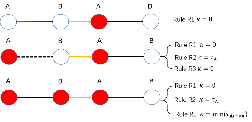
FIG. 1: Three possible ways to generate a new AIE. Red and white circles represent infected and susceptible nodes, respectively, whereas solid and dashed lines indicate active and dormant edges, respectively. We also show how to define the onset of the infection from A to B for the three rules used in this paper. Rule 1 sets this time always to zero. Rule 2 assigns to the newborn AIE the infected dwell time of node A. In Rule 3, the onset of the infection is set as the minimum between the infected dwell time of node A and the active dwell time of the edge connecting nodes A and B.

3 Non-Markovian Mean-field approach

Here, we extend the mean field approximation developed in Ref.[26] for static networks to the case of the temporal networks described in the previous section. Due to the non-Markovia dynamics, to describe the temporal evolution of the epidemic we have to keep track of the dwell time of nodes in each state, infected or susceptible. We then define $I_{i}(\tau;t)d\tau$ as the probability to find node $i$ infected at time $t$ and that, simultaneously, the time since it became infected is within the interval $(\tau,\tau+d\tau)$. Similarly, we define $S_{i}(\tau;t)$ as the probability to find node $i$ susceptible at time $t$ and that, simultaneously, the time since it became susceptible is within the interval $(\tau,\tau+d\tau)$. Notice that functions $I_{i}(\tau;t)$ and $S_{i}(\tau;t)$ are probability densities with respect to the variable $\tau$ but not $t$, so that the prevalence of node $i$ at time $t$, $\rho_{i}(t)$, defined as the probability to find node $i$ infected at time $t>0$ is

$$\rho_{i}(t)=\int_{0}^{t}I_{i}(\tau;t)d\tau,$$ (5)

and the global prevalence $\rho(t)=N^{-1}\sum_{i=1}^{N}\rho_{i}(t)$. Hereafter, as initial conditions, we assume that node $i$ is infected at time $t=0$ with probability $\rho_{i}(t=0)=\rho_{i,0}$.

Assuming that the infections from different edges are statistically independent events and working at the mean field level, in Ref.[26] it was shown that functions $I_{i}(\tau;t)$ and $S_{i}(\tau;t)$ satisfy the partial differential equations

$$\left(\frac{\partial}{\partial\tau}+\frac{\partial}{\partial t}\right)I_{i}(\tau;t)=-\omega_{\text{rec}}(\tau)I_{i}(\tau;t)$$ (6)

and

$$\left(\frac{\partial}{\partial\tau}+\frac{\partial}{\partial t}\right)S_{i}(\tau;t)=-\sum_{j=1}^{N}a_{ij}\phi_{i\leftarrow j}(\tau;t)S_{i}(\tau;t)$$ (7)

where $\phi_{i\leftarrow j}(\tau;t)$ is the instantaneous infection rate from node $j$ to $i$, which depend on the specific rule used and the on-off dynamics on the edges. Equations (6) and (7) are supplemented by the boundary conditions

$$S_{i}(0;t)=\int_{0}^{t}\omega_{\text{rec}}(\tau)I_{i}(\tau;t)d\tau$$ (8)

and

$$I_{i}(0;t)=\sum_{j=1}^{N}a_{ij}\int_{0}^{t}S_{i}(\tau;t)\phi_{i\leftarrow j}(\tau;t)d\tau,$$ (9)

Notice that these boundary conditions are slightly different from the ones in Ref.[26] because we consider that dwell times are bounded in the interval $\tau\in(0,t)$.

Finally, to close these equations, we need to find an expression for the instantaneous infection rate from node $j$ to susceptible node $i$ (with susceptible dwell time $\tau$) at time $t$, $\phi_{i\leftarrow j}(\tau;t)$. This rate depends on the particular rule used to determine the onset of the infection event. For R1, this time is the smallest between the susceptible dwell time of node $i$, the infected dwell time of node $j$, and the active dwell time of the edge connecting nodes $i$ and $j$. Thus, we can write

$$\phi_{i\leftarrow j}^{\text{R1}}(\tau;t)=P_{\text{on}}\int_{0}^{\infty}d\tau^{\prime}\frac{\Phi_{\text{on}}(\tau^{\prime})}{\langle\tau_{\text{on}}\rangle}\int_{0}^{t}d\tau^{\prime\prime}I_{j}(\tau^{\prime\prime};t)\omega_{\text{inf}}\left(\min{(\tau,\tau^{\prime},\tau^{\prime\prime})}\right)$$ (10)

For R2, the onset of the infection event is determined by the dwell time in the infected state of node $j$ at time $t$. Therefore, we write

$$\phi_{i\leftarrow j}^{\text{R2}}(\tau;t)=\phi_{i\leftarrow j}^{\text{R2}}(t)=P_{\text{on}}\int_{0}^{t}d\tau^{\prime\prime}I_{j}(\tau^{\prime\prime};t)\omega_{\text{inf}}\left(\tau^{\prime\prime}\right).$$ (11)

For R3, this time is the smaller between the infected dwell time of node $j$, and the active dwell time of the edge connecting nodes $i$ and $j$. Thus, we have

$$\phi_{i\leftarrow j}^{\text{R3}}(\tau;t)=\phi_{i\leftarrow j}^{\text{R3}}(t)=P_{\text{on}}\int_{0}^{\infty}d\tau^{\prime}\frac{\Phi_{\text{on}}(\tau^{\prime})}{\langle\tau_{\text{on}}\rangle}\int_{0}^{t}d\tau^{\prime\prime}I_{j}(\tau^{\prime\prime};t)\omega_{\text{inf}}\left(\min{(\tau^{\prime},\tau^{\prime\prime})}\right)$$ (12)

The set of equations Eqs. (5)- (12) form a closed set of equations that enable to find the temporal evolution of the prevalence $\rho_{i}(t)$ at the mean field level, as shown in Fig. 2. From this analysis, we already conclude that the only influence of the off-distribution $\varphi_{\text{\text{off}}}(\tau)$ on the SIS dynamics is through its average value, which affect the probability to find an edge in the on-state $P_{\text{on}}$.

It is illustrative to see how this formalism recovers the Markovian SIS model at the mean field level for static networks. In that case, $\omega_{\text{rec}}(\tau)=\delta$, $\omega_{\text{inf}}(\tau)=\lambda$ and $P_{\text{on}}=1$. Integrating Eq. (6) with respect to $\tau\in(0,t)$ leads to the differential equation

$$\frac{d\rho_{i}(t)}{dt}=-\delta\rho_{i}(t)+I_{i}(0;t)=-\delta\rho_{i}(t)+\sum_{j=1}^{N}a_{ij}\int_{0}^{t}S_{i}(\tau;t)\phi_{i\leftarrow j}(\tau;t)d\tau$$ (13)

In the Markovian case, the instantaneous infection rate from node $j$ to $i$ is independent of the rule used and takes the simple form

$$\phi_{i\leftarrow j}^{\text{R1}}(\tau;t)=\phi_{i\leftarrow j}^{\text{R2}}(\tau;t)=\phi_{i\leftarrow j}^{\text{R3}}(\tau;t)=\lambda\rho_{j}(t).$$ (14)

Using this result in Eq. (13) we obtain

$$\frac{d\rho_{i}(t)}{dt}=-\delta\rho_{i}(t)+\lambda\sum_{j=1}^{N}a_{ij}[1-\rho_{i}(t)]\rho_{j}(t),$$ (15)

which is the mean field approximation of the SIS model developed in Ref. [42]. At the steady state, the prevalence satisfy

$$\rho_{i}^{\text{st}}=\lambda_{\text{eff}}\sum_{j=1}^{N}a_{ij}[1-\rho_{i}^{\text{st}}]\rho_{j}^{\text{st}}.$$ (16)

with $\lambda_{\text{eff}}=\lambda/\delta$.

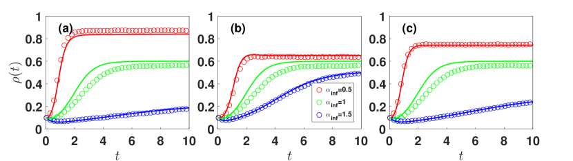
FIG. 2: Comparison between simulation and theoretical results of the temporal evolution of the density of infected nodes $\rho(t)$ on a random-regular network with $N=10000$ and $\langle k\rangle=10$ for rules R1 (a), R2 (b), and R3 (c). Red circles, green squares, and blue triangles represent the simulation results for $\alpha_{\text{inf}}=0.5,1,$ and $1.5$, respectively and solid lines are theoretical results. Other parameters are $\langle\tau_{\text{off}}\rangle=\langle\tau_{\text{on}}\rangle=1,\alpha_{\text{off}}=\alpha_{\text{on}}=5$, $u=0.5$ and $\delta=1$.

3.1 The steady state solution

At the steady state, functions $I_{i}(\tau;t)$, $S_{i}(\tau;t)$, and $\phi_{i\leftarrow j}(\tau;t)$ become independent of $t$ and we can find the following explicit expressions from Eqs. (6) and (7)

$$I_{i}^{\text{st}}(\tau)=\frac{\rho_{i}^{\text{st}}}{\langle\tau_{\text{rec}}\rangle}\Phi_{\text{\text{rec}}}(\tau)\;\;\text{and}\;\;S_{i}^{\text{st}}(\tau)=\frac{\rho_{i}^{\text{st}}}{\langle\tau_{\text{rec}}\rangle}\exp{\left(-\sum_{j}a_{ij}\int_{0}^{\tau}\phi_{i\leftarrow j}^{\text{st}}(\tau^{\prime})d\tau^{\prime}\right)}.$$ (17)

Integrating the last equation we obtain

$$1-\rho_{i}^{\text{st}}=\frac{\rho_{i}^{\text{st}}}{\langle\tau_{\text{rec}}\rangle}\int_{0}^{\infty}\exp{\left(-\sum_{j}a_{ij}\int_{0}^{\tau}\phi_{i\leftarrow j}^{\text{st}}(\tau^{\prime})d\tau^{\prime}\right)}d\tau.$$ (18)

Notice that combining the expression for $I_{i}^{\text{st}}(\tau)$ in Eq. (17) and the general expression for $\phi_{i\leftarrow j}(\tau;t)$, we can write that, at the steady state, $\phi_{i\leftarrow j}^{\text{st}}(\tau)=\frac{\rho_{j}^{\text{st}}P_{\text{on}}}{\langle\tau_{\text{rec}}\rangle}f(\tau)$, where $f(\tau)$ is a function that depends on the particular rule used but does not depend on the states of nodes $i$ and $j$. Thus, Eqs. (18) form set of closed equations for $\rho_{i}^{\text{st}}$ $\forall i=1,\cdots,N$.

To go further, we need to specify the particular rule used. In the case of R2, function $f(\tau)$ is independent of $\tau$, taking the value

$$f(\tau)=\int_{0}^{\infty}d\tau^{\prime\prime}\Phi_{\text{rec}}(\tau^{\prime\prime})\omega_{\text{inf}}(\tau^{\prime\prime}).$$ (19)

Using this result, Eq. (18) reduces to

$$\rho_{i}^{\text{st}}=\lambda_{\text{eff}}^{R2}\sum_{j=1}^{N}a_{ij}[1-\rho_{i}^{\text{st}}]\rho_{j}^{\text{st}},$$ (20)

with

$$\lambda_{\text{eff}}^{R2}=P_{\text{on}}\int_{0}^{\infty}\Phi_{\text{\text{rec}}}(\tau)\frac{\varphi_{\text{\text{inf}}}(\tau)}{\Phi_{\text{\text{inf}}}(\tau)}d\tau.$$ (21)

Equation (20) is identical to the mean field steady state of the non-Markovian SIS model in Eq. (16) but with an effective infection rate given by $\lambda_{\text{eff}}^{R2}$ so that, at the steady state, we can replace a non-Markovian SIS epidemic process on a temporal network by a Markovian one on a static network. It is also interesting to notice that, for rule R2, the effect of the temporal nature of the network has only a minor effect on the dynamics through the probability $P_{\text{on}}$. However, the particular details of the on-off dynamics are very relevant to determine the time needed to reach the steady state, or the time window one must observe the system to make sure that the steady state is sufficiently sampled.

In the case of R3, function $f(\tau)$ is also independent of $\tau$ and takes the form

$$f(\tau)=\int_{0}^{\infty}d\tau^{\prime}\frac{\Phi_{\text{on}}(\tau^{\prime})}{\langle\tau_{\text{on}}\rangle}\int_{0}^{\infty}d\tau^{\prime\prime}\Phi_{\text{rec}}(\tau^{\prime\prime})\omega_{\text{inf}}\left(\min{(\tau^{\prime},\tau^{\prime\prime})}\right),$$ (22)

so that Eq. (18) reduces to

$$\rho_{i}^{\text{st}}=\lambda_{\text{eff}}^{R3}\sum_{j=1}^{N}a_{ij}[1-\rho_{i}^{\text{st}}]\rho_{j}^{\text{st}},$$ (23)

with

$$\lambda_{\text{eff}}^{R3}=P_{\text{on}}\int_{0}^{\infty}\frac{\Phi_{\text{on}}(\tau^{\prime})}{\langle\tau_{\text{on}}\rangle}d\tau^{\prime}\int_{0}^{\infty}\Phi_{\text{rec}}(\tau^{\prime\prime})\omega_{\text{inf}}(\min(\tau^{\prime},\tau^{\prime\prime}))d\tau^{\prime\prime}.$$ (24)

As in the previous case, the steady state of the non-Markovian SIS dynamics under R3 can be reduced to the Markovian case with the effective infection rate $\lambda_{\text{eff}}^{R3}$. Unlike R2, here the on-off dynamics of edges plays a more relevant role because the distribution of dwell times of edged in the on state has a strong influence on the definition of the effective rate $\lambda_{\text{eff}}^{R3}$.

In the case of rule R1, function $f(\tau)$ is not constant and it is not possible to reduce the steady state to the non-Markovian case. Besides, in this case, the assumption about the independence between different infectious channels does not hold. We can understand this phenomenon with a simple example: consider an infected node A with three infected neighbors B, C, and D, connected by active edges. If node A recovers, then the infections from nodes B, C, and D to now susceptible node A will start simultaneously and, therefore, become strongly correlated. However, it is still possible to find an effective infection rate that becomes exact near the phase transition. Indeed, in this case the density of infected nodes is very low and the number of infected neighbors is small so that the correlations between different edges become irrelevant. We can then use the formalism in Ref. [24], where the effective infection rate from node $j$ to $i$ is defined as

$$\lambda_{\text{eff}}=P_{\text{on}}\langle\tau_{\text{rec}}\rangle\langle\omega_{\text{inf}}(\tau)|\text{node $i$ susceptible, $j$ infected, edge $ij$ active}\rangle,$$ (25)

where $\tau$ is the time since the infection process started given that node $i$ is susceptible, $j$ infected, and the edge between them active. For rule R1 at the steady state, the only information about this time is that it must be shorter than the time $j$ takes to infect $i$, also shorter than the time $j$ takes to recover, and shorter than the time edge $ij$ remains in the active state. Therefore, the pdf of this time is given by

$$\psi(\tau|\text{node $i$ susceptible, $j$ infected, edge $ij$ active})=\frac{\Phi_{\text{inf}}(\tau)\Phi_{\text{rec}}(\tau)\Phi_{\text{on}}(\tau)}{\int_{0}^{\infty}\Phi_{\text{inf}}(\tau)\Phi_{\text{rec}}(\tau)\Phi_{\text{on}}(\tau)d\tau}$$ (26)

and the effective infection rate for rule R1 becomes

$$\lambda_{\text{eff}}^{R1}=P_{\text{on}}\langle\tau_{\text{rec}}\rangle\frac{\int_{0}^{\infty}\varphi_{\text{inf}}(\tau)\Phi_{\text{rec}}(\tau)\Phi_{\text{on}}(\tau)d\tau}{\int_{0}^{\infty}\Phi_{\text{inf}}(\tau)\Phi_{\text{rec}}(\tau)\Phi_{\text{on}}(\tau)d\tau}.$$ (27)

We then expect that near the critical point, the behavior of the non-Markovian SIS on a temporal network is equivalent to the Markovian SIS on a static network with the effective infection rate $\lambda_{\text{eff}}^{R1}$. Then, we can use the expression in Eq. (27) to find the exact position of the critical point in terms of the critical point of the non-Markovian SIS on the static version of the network.

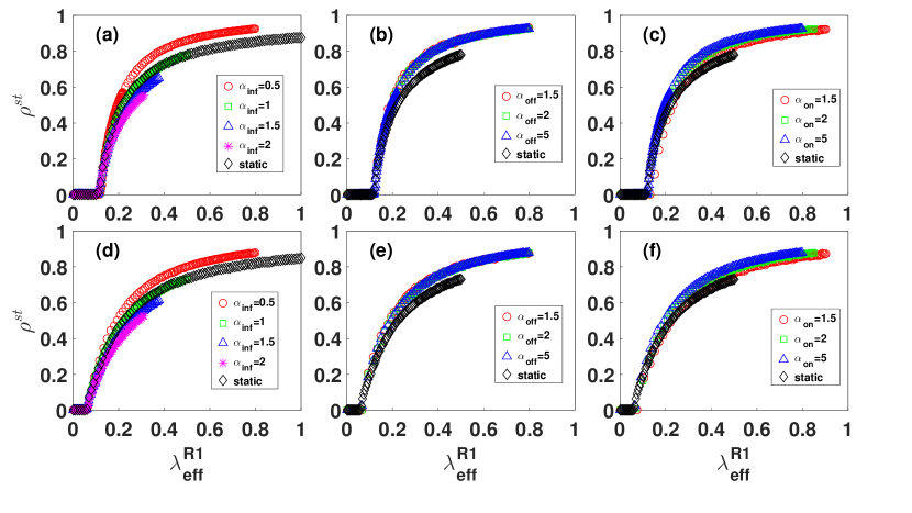
FIG. 3: Steady-state prevalence $\rho^{\text{st}}$ under rule R1 as a function of $\lambda_{\text{eff}}^{R1}$ in Eq. (27) for different values of the parameters $\alpha_{\text{inf}}$, $\alpha_{\text{off}}$ and $\alpha_{\text{on}}$. Panels (a), (b), and (c) show results for Erdős-Rényi networks with $\langle k\rangle=10$ and size $N=10000$. Panels (d), (e), and (f) show results of Barabási-Albert networks with $N=10000$. In panels (a) and (d) we fix $\alpha_{\text{off}}=5$, $\alpha_{\text{on}}=5$ and change $\alpha_{\text{inf}}$. In panels (b) and (e) we fix $\alpha_{\text{inf}}=0.5$, $\alpha_{\text{on}}=5$ and change $\alpha_{\text{off}}$. Finally, in panels (c) and (f) we fix $\alpha_{\text{inf}}=0.5$, $\alpha_{\text{off}}=5$ and change $\alpha_{\text{on}}$. In all cases, we set $\langle\tau_{\text{off}}\rangle=\langle\tau_{\text{on}}\rangle=1$, $u=0.5$, and $\delta=1$. Black empty diamonds correspond to the Markovian SIS dynamic on the static version of the network with the infection rate $\lambda_{\text{eff}}^{R1}$.

4 Simulation Results

We check the validity of the theory developed in the previous section by means of extensive numerical simulations of the non-Markovian SIS dynamics on temporal networks. As suggested by empirical observations, we consider both the dormant and active times of edges to be power law distributed. Specifically, we use the Lomax distribution  [43] as

$$\varphi(\tau)=\frac{\alpha\xi^{\alpha}}{(\tau+\xi)^{(1+\alpha)}},$$ (28)

with exponent $\alpha>1$ and $\xi=(\alpha-1)\langle\tau\rangle$. Infections are modeled with a Weibull distribution with shape parameter $\alpha_{\text{inf}}$ and scale parameter $u$.

$$\varphi_{\text{inf}}(\tau)=\alpha_{\text{inf}}u^{\alpha_{\text{inf}}}\tau^{\alpha_{\text{inf}}-1}e^{-(u\tau)^{\alpha_{\text{inf}}}}.$$ (29)

This is a useful choice that interpolates between a strongly picked distribution when $\alpha_{\text{inf}}>1$ to a long tailed distribution when $\alpha_{\text{inf}}<1$, recovering the Markovian case when $\alpha_{\text{inf}}=1$. Finally, we consider a Markovian recovery process with rate $\delta$, $\varphi_{\text{rec}}(\tau)=\delta e^{-\delta\tau}$.

We first check the ability of our formalism to describe the short term temporal evolution of the dynamics. Specifically, we perform numerical simulations initially infecting $10\%$ of nodes in the network. Figure 2 shows results from numerical simulations for the three rules compared to the numerical solution of Eqs. (5)- (12). As it can be observed, the non-Markovian mean field approach agrees very well with numerical simulations. In particular, it is able to predict the characteristic time scale to reach the steady state and a non trivial non-monotonous behavior when the probability density of infection times is picked around it average (so that $\alpha_{\text{inf}}>1$).

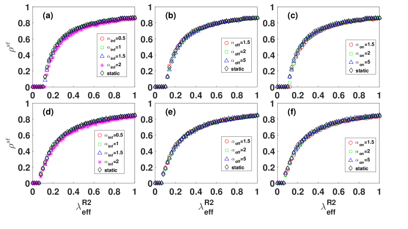
FIG. 4: Steady-state prevalence $\rho^{\text{st}}$ under rule R2 as a function of $\lambda_{\text{eff}}^{R2}$ in Eq. (21)) for different values of the parameters $\alpha_{\text{inf}}$, $\alpha_{\text{off}}$ and $\alpha_{\text{on}}$. Panels (a), (b), and (c) show results for Erdős-Rényi networks with $\langle k\rangle=10$ and size $N=10000$. Panels (d), (e), and (f) show results of Barabási-Albert networks with $N=10000$. In panels (a) and (d) we fix $\alpha_{\text{off}}=5$, $\alpha_{\text{on}}=5$ and change $\alpha_{\text{inf}}$. In panels (b) and (e) we fix $\alpha_{\text{inf}}=0.5$, $\alpha_{\text{on}}=5$ and change $\alpha_{\text{off}}$. Finally, in panels (c) and (f) we fix $\alpha_{\text{inf}}=0.5$, $\alpha_{\text{off}}=5$ and change $\alpha_{\text{on}}$. In all cases, we set $\langle\tau_{\text{off}}\rangle=\langle\tau_{\text{on}}\rangle=1$, $u=0.5$, and $\delta=1$. Black empty diamonds correspond to the Markovian SIS dynamic on the static version of the network with the infection rate $\lambda_{\text{eff}}^{R2}$.

Next, we study the steady state of the dynamics and compare numerical simulations with different values of the parameters of the SIS dynamics and the temporal network. Figure 3 shows the steady prevalence as a function of the effective infection rate for rule R1, $\lambda_{\text{eff}}^{R1}$. As discussed above, the prevalence for different values of the parameters do not colapse into a single curve, which indicates that the non-Markovian SIS model cannot be reduced to the Markovian case under rule R1. However, all curves do colapse nicely when the prevalence approaches zero. This means that, as predicted, the effective infection rate $\lambda_{\text{eff}}^{R1}$ is able to recover the exact value of the epidemic threshold in terms of the epidemic threshold of the Markovian dynamics on the static version of the network. The situation is different in the case of rules R2 and R3. In both cases, our theory predicts that the non-Markovian dynamics can be reduced to the Markovian one on a static network with effective infection rates $\lambda_{\text{eff}}^{R2}$ and $\lambda_{\text{eff}}^{R3}$. Figures 4 and 5 show numerical simulations for rules R2 and R3 where the colapse of the different prevalence curves is evident, thus corroborating our predictions.

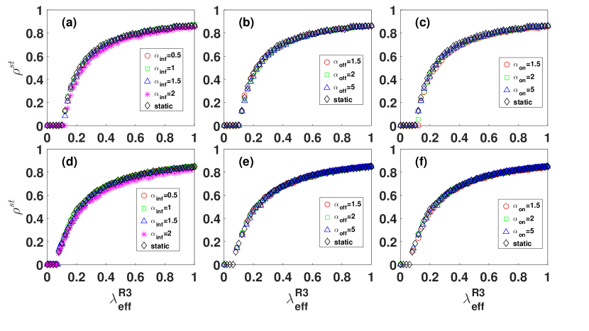
FIG. 5: Steady-state prevalence $\rho^{\text{st}}$ under rule R3 as a function of $\lambda_{\text{eff}}^{R3}$ in Eq. (24)) for different values of the parameters $\alpha_{\text{inf}}$, $\alpha_{\text{off}}$ and $\alpha_{\text{on}}$. Panels (a), (b), and (c) show results for Erdős-Rényi networks with $\langle k\rangle=10$ and size $N=10000$. Panels (d), (e), and (f) show results of Barabási-Albert networks with $N=10000$. In panels (a) and (d) we fix $\alpha_{\text{off}}=5$, $\alpha_{\text{on}}=5$ and change $\alpha_{\text{inf}}$. In panels (b) and (e) we fix $\alpha_{\text{inf}}=0.5$, $\alpha_{\text{on}}=5$ and change $\alpha_{\text{off}}$. Finally, in panels (c) and (f) we fix $\alpha_{\text{inf}}=0.5$, $\alpha_{\text{off}}=5$ and change $\alpha_{\text{on}}$. In all cases, we set $\langle\tau_{\text{off}}\rangle=\langle\tau_{\text{on}}\rangle=1$, $u=0.5$, and $\delta=1$. Black empty diamonds correspond to the Markovian SIS dynamic on the static version of the network with the infection rate $\lambda_{\text{eff}}^{R3}$.

5 Conclusion and Discussion

Empirical evidence demonstrates that non-Markovian dynamics and temporal networks are prevalent in real complex systems. However, these properties, particularly those associated with memory effects, are frequently overlooked in scientific literature. This is partially due to the analytical and computational challenges that these properties entail, but the major obstacle when dealing with non-Markovian dynamics is our lack of knowledge about how memory is implemented. In this study, we explored three different possibilities, but numerous other possibilities exist, and it is challenging to determine which ones apply to actual systems. This has significant consequences because, as our work has shown, the specifics of the rule utilized dictate the fate of the dynamics. We have demonstrated that some of these rules are “simple” in that an effective parameter can encode the non-Markovian and temporal properties of the dynamics. However, in other cases, this is only possible near the critical point, allowing us to recover the critical threshold of the dynamics. In light of these findings, it is uncertain whether the concept of universality class can be extended to general non-Markovian dynamics.

6 Acknowledgments

This work was supported by the National ten thousand talents plan youth top talent project, the National Natural Science Foundation of China (Grant Nos. 11975099, 12231012, 11875132), the Science and Technology Commission of Shanghai Municipality (Grant No.22DZ2229004) and the China Scholarship Council (Grant No. 202006140147). M. B. acknowledge support from: Grant TED2021-129791B-I00 funded by MCIN/AEI/10.13039/501100011033 and the “European Union NextGenerationEU/PRTR”’; Grant PID2019-106290GB-C22 funded by
MCIN/AEI/10.13039/501100011033; Generalitat de Catalunya grant number 2021SGR00856 and the ICREA Academia award, funded by the Generalitat de Catalunya.

References

References

-
[1]
R. Pastor-Satorras, C. Castellano, P. Van Mieghem, A. Vespignani,
Epidemic processes
in complex networks, Rev. Mod. Phys. 87 (2015) 925–979.
doi:10.1103/RevModPhys.87.925.
URL https://link.aps.org/doi/10.1103/RevModPhys.87.925 - [2] R. M. Anderson, R. M. May, Infectious diseases of humans: dynamics and control, Oxford university press, 1992.
- [3] C. H. Weiss, J. Poncela-Casasnovas, J. I. Glaser, A. R. Pah, S. D. Persell, D. W. Baker, R. G. Wunderink, L. A. N. Amaral, Adoption of a high-impact innovation in a homogeneous population, Physical review x 4 (4) (2014) 041008.
- [4] E. M. Rogers, A. Singhal, M. M. Quinlan, Diffusion of innovations, in: An integrated approach to communication theory and research, Routledge, 2014, pp. 432–448.
- [5] L. Wang, M. Wu, X. Xu, W. Fan, The diffusion of intelligent manufacturing applications based sir model, Journal of Intelligent & Fuzzy Systems 38 (6) (2020) 7725–7732.
- [6] G. Fibich, Bass-sir model for diffusion of new products in social networks, Physical Review E 94 (3) (2016) 032305.
- [7] S. Bikhchandani, D. Hirshleifer, I. Welch, A theory of fads, fashion, custom, and cultural change as informational cascades, Journal of political Economy 100 (5) (1992) 992–1026.
- [8] A. V. Banerjee, A simple model of herd behavior, The quarterly journal of economics 107 (3) (1992) 797–817.
- [9] P. S. Dodds, D. J. Watts, Universal behavior in a generalized model of contagion, Physical review letters 92 (21) (2004) 218701.
- [10] P. Sheridan Dodds, D. J. Watts, A generalized model of social and biological contagion, arXiv e-prints (2017) arXiv–1705.
-
[11]
M. Boguñá, C. Castellano, R. Pastor-Satorras,
Nature of the
epidemic threshold for the susceptible-infected-susceptible dynamics in
networks, Phys. Rev. Lett. 111 (2013) 068701.
doi:10.1103/PhysRevLett.111.068701.
URL https://link.aps.org/doi/10.1103/PhysRevLett.111.068701 -
[12]
M. A. Serrano, D. Krioukov, M. Boguñá,
Percolation in
self-similar networks, Phys. Rev. Lett. 106 (2011) 048701.
doi:10.1103/PhysRevLett.106.048701.
URL https://link.aps.org/doi/10.1103/PhysRevLett.106.048701 - [13] M. Salathé, J. H. Jones, Dynamics and control of diseases in networks with community structure, PLoS computational biology 6 (4) (2010) e1000736.
- [14] N. T. Bailey, Significance tests for a variable chance of infection in chain-binomial theory, Biometrika (1956) 332–336.
- [15] M. Eichner, K. Dietz, Transmission potential of smallpox: estimates based on detailed data from an outbreak, American journal of epidemiology 158 (2) (2003) 110–117.
- [16] H. Nishiura, M. Eichner, Infectiousness of smallpox relative to disease age: estimates based on transmission network and incubation period, Epidemiology & Infection 135 (7) (2007) 1145–1150.
- [17] G. Chowell, H. Nishiura, Transmission dynamics and control of ebola virus disease (evd): a review, BMC medicine 12 (1) (2014) 1–17.
- [18] S. A. Lauer, K. H. Grantz, Q. Bi, F. K. Jones, Q. Zheng, H. R. Meredith, A. S. Azman, N. G. Reich, J. Lessler, The incubation period of coronavirus disease 2019 (covid-19) from publicly reported confirmed cases: estimation and application, Annals of internal medicine 172 (9) (2020) 577–582.
- [19] J. Qin, C. You, Q. Lin, T. Hu, S. Yu, X.-H. Zhou, Estimation of incubation period distribution of covid-19 using disease onset forward time: a novel cross-sectional and forward follow-up study, Science advances 6 (33) (2020) eabc1202.
- [20] C. McAloon, Á. Collins, K. Hunt, A. Barber, A. W. Byrne, F. Butler, M. Casey, J. Griffin, E. Lane, D. McEvoy, et al., Incubation period of covid-19: a rapid systematic review and meta-analysis of observational research, BMJ open 10 (8) (2020) e039652.
- [21] P. Holme, J. Saramäki, Temporal networks, Physics reports 519 (3) (2012) 97–125.
- [22] P. Holme, Modern temporal network theory: a colloquium, The European Physical Journal B 88 (9) (2015) 1–30.
- [23] R. Lambiotte, N. Masuda, A guide to temporal networks, Vol. 4, World Scientific, 2016.
- [24] M. Starnini, J. P. Gleeson, M. Boguñá, Equivalence between non-markovian and markovian dynamics in epidemic spreading processes, Physical review letters 118 (12) (2017) 128301.
- [25] V. Shkilev, Non-markovian edge-based compartmental modeling, Physical Review E 99 (4) (2019) 042408.
- [26] M. Feng, S.-M. Cai, M. Tang, Y.-C. Lai, Equivalence and its invalidation between non-markovian and markovian spreading dynamics on complex networks, Nature communications 10 (1) (2019) 1–10.
- [27] P. Van Mieghem, R. Van de Bovenkamp, Non-markovian infection spread dramatically alters the susceptible-infected-susceptible epidemic threshold in networks, Physical review letters 110 (10) (2013) 108701.
- [28] Z.-H. Lin, M. Feng, M. Tang, Z. Liu, C. Xu, P. M. Hui, Y.-C. Lai, Non-markovian recovery makes complex networks more resilient against large-scale failures, Nature communications 11 (1) (2020) 1–10.
- [29] L. Böttcher, N. Antulov-Fantulin, Unifying continuous, discrete, and hybrid susceptible-infected-recovered processes on networks, Physical Review Research 2 (3) (2020) 033121.
-
[30]
X. R. Hoffmann, M. Boguñá,
Memory-induced complex
contagion in epidemic spreading, New Journal of Physics 21 (3) (2019)
033034.
doi:10.1088/1367-2630/ab0aa6.
URL https://dx.doi.org/10.1088/1367-2630/ab0aa6 -
[31]
N. Perra, B. Gonçalves, R. Pastor-Satorras, A. Vespignani,
Activity driven modeling of time
varying networks, Scientific Reports 2 (1) (2012) 469.
doi:10.1038/srep00469.
URL https://doi.org/10.1038/srep00469 - [32] A. Barrat, B. Fernandez, K. K. Lin, L.-S. Young, Modeling temporal networks using random itineraries, Physical review letters 110 (15) (2013) 158702.
- [33] M. Karsai, N. Perra, A. Vespignani, Time varying networks and the weakness of strong ties, Scientific reports 4 (1) (2014) 1–7.
- [34] K. Sun, A. Baronchelli, N. Perra, Contrasting effects of strong ties on sir and sis processes in temporal networks, The European Physical Journal B 88 (12) (2015) 1–8.
- [35] P. Holme, Temporal network structures controlling disease spreading, Physical Review E 94 (2) (2016) 022305.
- [36] I. Scholtes, N. Wider, R. Pfitzner, A. Garas, C. J. Tessone, F. Schweitzer, Causality-driven slow-down and speed-up of diffusion in non-markovian temporal networks, Nature communications 5 (1) (2014) 1–9.
-
[37]
E. Ortiz, M. Starnini, M. Á. Serrano,
Navigability of temporal
networks in hyperbolic space, Scientific Reports 7 (1) (2017) 15054.
doi:10.1038/s41598-017-15041-0.
URL https://doi.org/10.1038/s41598-017-15041-0 -
[38]
G. García-Pérez, M. Boguñá, M. Á. Serrano,
Regulation of burstiness by
network-driven activation, Scientific Reports 5 (1) (2015) 9714.
doi:10.1038/srep09714.
URL https://doi.org/10.1038/srep09714 - [39] S. Unicomb, G. Iñiguez, J. P. Gleeson, M. Karsai, Dynamics of cascades on burstiness-controlled temporal networks, Nature communications 12 (1) (2021) 1–10.
-
[40]
M. B. ná, A. Berezhkovskii, G. Weiss,
Residence
time densities for non-markovian systems. (i). the two-state system, Physica
A: Statistical Mechanics and its Applications 282 (3) (2000) 475–485.
doi:https://doi.org/10.1016/S0378-4371(00)00091-1.
URL https://www.sciencedirect.com/science/article/pii/S0378437100000911 -
[41]
M. Boguñá, L. F. Lafuerza, R. Toral, M. A. Serrano,
Simulating
non-markovian stochastic processes, Phys. Rev. E 90 (2014) 042108.
doi:10.1103/PhysRevE.90.042108.
URL https://link.aps.org/doi/10.1103/PhysRevE.90.042108 - [42] P. Van Mieghem, J. Omic, R. Kooij, Virus spread in networks, IEEE/ACM Transactions On Networking 17 (1) (2008) 1–14.
- [43] M. Mancastroppa, A. Vezzani, M. A. Muñoz, R. Burioni, Burstiness in activity-driven networks and the epidemic threshold, Journal of Statistical Mechanics: Theory and Experiment 2019 (5) (2019) 053502.