GETNext: Trajectory Flow Map Enhanced Transformer for Next POI Recommendation

Abstract.

Next POI recommendation intends to forecast users’ immediate future movements given their current status and historical information, yielding great values for both users and service providers. However, this problem is perceptibly complex because various data trends need to be considered together. This includes the spatial locations, temporal contexts, user’s preferences, etc. Most existing studies view the next POI recommendation as a sequence prediction problem while omitting the collaborative signals from other users. Instead, we propose a user-agnostic global trajectory flow map and a novel Graph Enhanced Transformer model (GETNext) to better exploit the extensive collaborative signals for a more accurate next POI prediction, and alleviate the cold start problem in the meantime. GETNext incorporates the global transition patterns, user’s general preference, spatio-temporal context, and time-aware category embeddings together into a transformer model to make the prediction of user’s future moves. With this design, our model outperforms the state-of-the-art methods with a large margin and also sheds light on the cold start challenges within the spatio-temporal involved recommendation problems.

1. Introduction

Location-Based Services (LBS) is gaining significant advancements in recent years owing to the prevalence of GPS-enabled mobile devices. Service providers such as Foursquare, Gowalla, or Yelp enable users to share their experiences, tips, and moments on points of interest (POIs). Large volumes of spatio-temporal data are being accumulated, as a result, giving rise to increasingly powerful next POI recommendation systems (Feng et al., 2015). Such systems aim to predict the next POI that users will visit given their current and historical footprints (i.e., check-ins). They not only help users to better explore their surroundings but also facilitate businesses to improve their advertising strategies (Jiang et al., 2015).

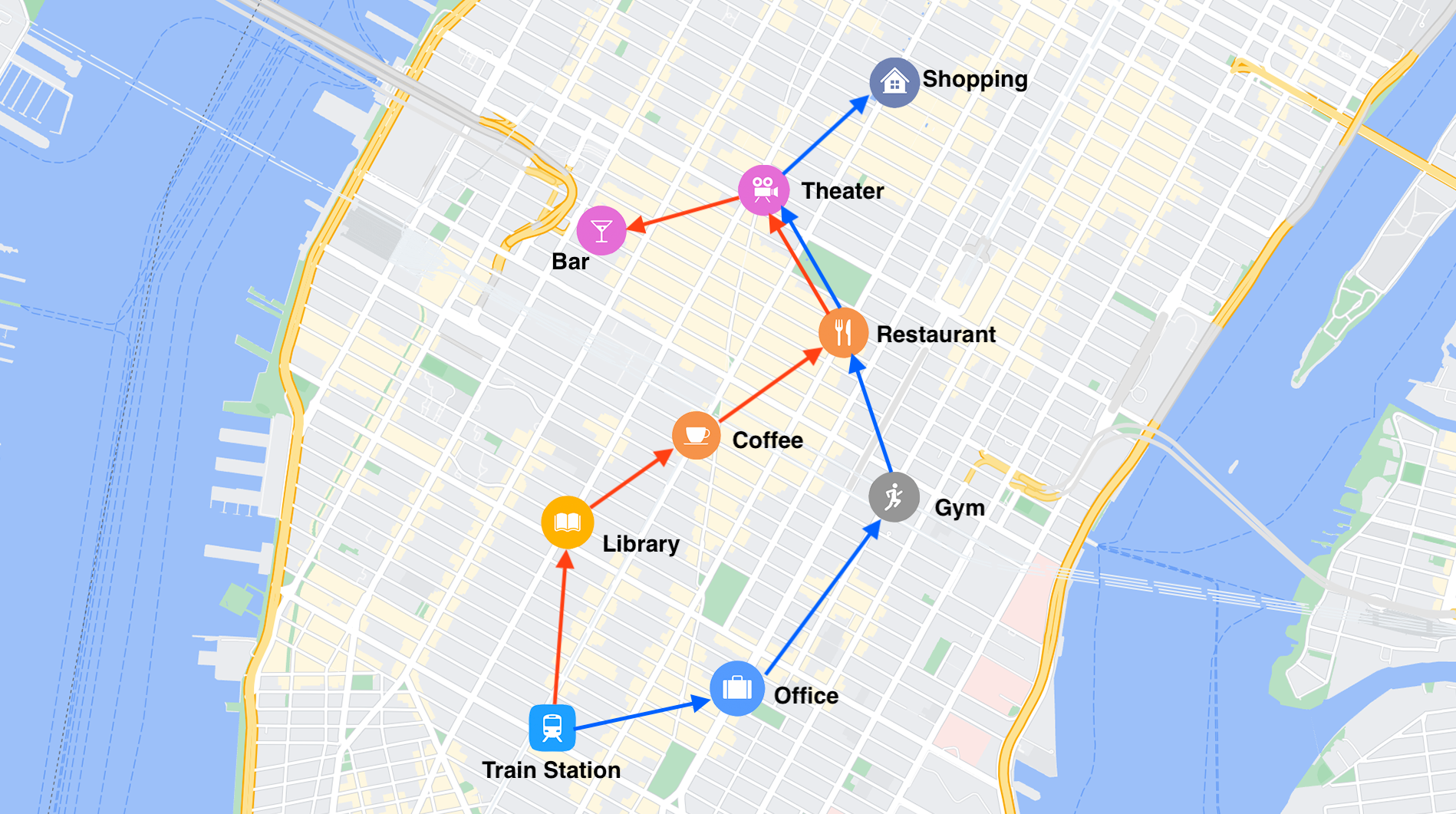
Figure 1. Two trajectories (red and blue) of two users in different days share the same fragment (restaurant to theater) in Manhattan, NYC

As (short-term) temporal patterns of a user’s trajectory provide critical insights in predicting the user’s future movements, the predominant approach treats next POI recommendation as a sequence prediction task. As a result, state-of-the-art models for this task employ various forms of recurrent neural networks (RNN) to encode spatio-temporal information (Liu et al., 2016b; Wu et al., 2019; Zhao et al., 2020a; Sun et al., 2020; Zhao et al., 2020b; Wu et al., 2020). There are, however, three limitations to this approach. First, the model performance drops significantly on short trajectories when compared with long trajectories. This is due to the limited spatio-temporal contexts provided by the short trajectories. Second, the recommendation accuracy for inactive users, who have only checked in a small number of POIs, is often low. It is a commonplace that cold-start problem exists in real-life recommender systems. Third, the POI category usually presents strong temporal correlations. For example, the check-in frequency of the train station is significantly higher on rush hours compared with midnight as shown in Figure 3. However, existing models fail to bridge the time and POI category. While no silver-bullet exists in tackling the first two problems due to inherent data scarcity issues, we argue that these limitations can be mitigated to some degree by harnessing collective information from other users. In particular, individuals tend to share certain fragments of check-in sequences, forming collective trajectory flows. For instance, two users went to the same restaurant and the same theater in the same order but on different days, as shown in Figure 1. These trajectory flows may provide crucial hints on the generic movement patterns of users, helping to resolve issues with short trajectories and inactive users. Nevertheless, utilizing these trajectory flows in next POI recommendation is not straightforward, as we need to address the following questions: (1) how to aggregate information from check-in sequences to form a unified representation of global trajectory flow patterns? (2) how to reserve the important spatio-temporal contextual information such as category information and user preference besides these trajectory flows? and (3) how to leverage all information above in next POI recommendation, to strike a balance between generic movement patterns and personalized demands?

For Question (1), we construct a novel (user-agnostic) trajectory flow map that summarizes trajectories between POIs as well as features of each POI in a single graph structure. More precisely, nodes in this graph are POIs with attributes including geographical location, category, and check-in counts. A directed edge connects a POI to another if they are successively visited in the same check-in trajectory, and edge weight represents their co-visit frequency. Different from the graphs designed for modeling the correlations between users and items in existing POI and product recommendation models, this trajectory flow map captures the transitional influence between POIs. Then to exploit the collective information in the trajectory flow map, we employ a graph convolutional network (GCN) to embed POIs into a latent space that preserves the global transitions among POIs. More precisely, the GCN updates the embedding of each node by aggregating from its in-neighbors’ embeddings. In this way, the embedding of each POI in the trajectory flow map will be influenced by its precedents, and thus the information of global transitions are well preserved. Consequently, without knowing the historical check-ins of a user, one can still recommend the most probable out-neighbor of the current POI. An underlying assumption behind the global trajectory flow map is that recommending the popular next POI may not be the best choice but is certainly improved from a random guess. In particular, using global trajectory flow map should improve top-$k$ accuracy for relatively large $k$. See Sec. 4.2.

For Question (2), the trajectory flow map mainly captures the user-agnostic POI transition patterns. Meanwhile, users’ preferences and spatio-temporal context are essential for personalized recommendations. The long-term preferences measure a user’s general tastes, such as the tendency to a favourite restaurant or a movie theater. The short-term preferences are reflected by the recent check-ins of the user, which provide a more concrete spatial-temporal context. Thus, we utilize the embedding layers to capture users’ general preference, POI category embeddings, and a time2vec model to depict time embeddings. Moreover, the POI categories usually show strong correlations with time. To bridging them together, category and time embeddings are merged and feed into a fusion module to produce the time-aware category context embedding. See Sec. 4.3.

Summarising the above, we propose a Graph Enhanced Transformer framework GETNext that unifies the generic movement patterns, user’s general preferences, short-term spatio-temporal contexts, and time-aware category embeddings to predict user’s next POIs. Compared with RNN and LSTM, transformer can learn the contribution of each check-in directly from the input trajectory to the final recommendation using the self-attention mechanism. In other words, the model may differentiate the informativeness of different check-ins and aggregate all check-ins in the trajectory simultaneously for prediction, yielding superior performance. In GETNext we adopt the transformer encoder with several multi-layer perceptron (MLP) decoders to integrate the implicit global flow patterns that encoded in POI embeddings and other personalized embeddings. Moreover, the global flow patterns are also explicitly injected to the final prediction by a learned transition attention map. This novel architecture answers Question (3) above. See Sec. 4.4.

To validate our proposed model, we conduct a series of experiments on well-known real-world datasets. Our experiment results show that GETNext are able to significantly outperform existing state-of-the-art methods. E.g., up to 11% in terms of top-5 accuracy on NYC dataset. See Section 5. We list main contributions of our work below:

1. We propose a global trajectory flow map to model the common visiting-order transition information, and utilize a graph convolutional network to encode them into POI embedding.

2. We develop a novel time-aware category context embedding to capture the diverse temporal patterns of POI categories.

3. We propose a transformer-based framework to integrate global transition patterns, user general tastes, user short term trajectory, and spatio-temporal context together for next POI recommendation.

2. Related Work

2.1. Next POI Recommendation

Compared with conventional POI recommendation, next POI recommendation (Cheng et al., 2013) focuses more on the temporal influence of the recent trajectory to predict a user’s next moves. Early studies adopt methods that have been widely used in other sequential recommendation tasks such as Markov chains (Cheng et al., 2013; Zhang et al., 2014; Ye et al., 2013). For instance, the pioneering work by Cheng et al. (Cheng et al., 2013) recommended next POIs using a matrix factorization method which embeds personalized Markov chains (FPMC) (Rendle et al., 2010). Likewise, Zhang et al. (Zhang et al., 2014) proposed an additive Markov chain to model the sequential transitive influence. Meanwhile, other studies explored the possibility of tailoring the commonly-used matrix factorization or metric embedding technique into the next POI recommendation (Feng et al., 2015; Zhao et al., 2016; Liu et al., 2016a). In general, these early methods are rather limited compared with deep neural networks models in terms of their abilities to model sequence data.

More recently, researchers turned to deep learning and advanced embedding methods (Feng et al., 2020). Variants of RNN were proposed to capture the temporal dynamics and sequential correlations (Liu et al., 2016b; Wu et al., 2019; Zhao et al., 2020a; Sun et al., 2020; Zhao et al., 2020b; Wu et al., 2020). In 2016, Liu et al. (Liu et al., 2016b) proposed spatial temporal recurrent neural networks (ST-RNN) which incorporated spatio-temporal contexts into RNN layers. In particular, the spatial contexts are represented by geographical distance transition matrices and time transition matrices encode temporal context. LSTM was also adopted to model user’s long- and short-term preferences. In LSPL (Wu et al., 2019) and PLSPL (Wu et al., 2020), the authors trained standard LSTM models for short-term trajectory mining, and general embedding layers to capture users’ preference. Zhao et al. (Zhao et al., 2020a) designed a novel LSTM unit called spatio-temporal gated network (STGN) with two time gates and two distance gates to model the time intervals and distance intervals in both short-term and long-term sequence. In general, all work above view the next POI recommendation as a sequential prediction task. There are also a few studies that adopted the attention mechanism into this recommendation task, such as DeepMove (Feng et al., 2018) and STAN (Luo et al., 2021). DeepMove (Feng et al., 2018) proposed an attention model to capture the multi-level periodicity pattern and a recurrent neural network modeling the sequential transitions for the final recommendation. STAN (Luo et al., 2021) employed the self-attention mechanism to extract the non-adjacent point-to-point interactions where sequential models fail to do. However, all of these studies overlooking the potential benefits of exploiting generic movements of users.

2.2. Graphs in Location-based Recommendation

In this paper, we aim to take advantage of graph-based methods in next POI recommendation. Graphs-based methods – such as those that utilise location-based social networks (LBSN) – provide a powerful paradigm especially for conventional (non-sequential) recommendation tasks. Indeed, (Yuan et al., 2014) built a geographical-temporal influences aware graph (GTAG) which is a tripartite graph consisting of POI, session, and user nodes. However, introducing the session nodes can lead to an explosion of graph size. Unlike GTAG, (Xie et al., 2016) constructed four bipartite graphs, including POI-POI, POI-Region, POI-Time and POI-Word interaction graphs, to capture sequential effect, geographical influence, temporal dynamics, and semantic features, respectively. The authors then extended LINE network embedding model (Tang et al., 2015) to bipartite graphs, and used conditional probability as well as other statistical tools to train graph embeddings. A similar work is GGLR (Chang et al., 2020), graph-based geographical latent representation model. GGLR utilizes POI-POI graph and POI-User graph. In POI-User bipartite graph, user nodes and POI nodes are connected if the user ever visited the POI in check-in history, which aims to highlight user’s preference.

We point out that all studies above are for conventional (not-“next”) POI recommendation problem. To our knowledge, no work exists that explicitly leverages a unified graph structure for next POI recommendation. In a recent work (Li et al., 2021), for each POI in a given check-in sequence, the authors randomly sampled previous and next check-ins from other check-in sequences and incorporated these POIs to train an embedding of the current POI. The aim was to capture local (one-hop) transition of POIs and thus the embedding does not explicitly reflect the global (multi-hop) transition patterns. Instead, our trajectory flow map is a unified graph structure that manifests global patterns among all POIs. In this sense, our model is the first that utilizes graph-based learning to encode generic transitional information of POIs in a next POI recommendation task.

3. Problem Formulation

Let $U=\{u_{1},u_{2},\cdots,u_{M}\}$ be a set of users, $P=\{p_{1},p_{2},\cdots,p_{N}\}$ be a set of POIs (such as specific restaurants, hotels) and $T=\{t_{1},t_{2},\cdots,t_{K}\}$ denotes the set of time stamps, where $M$, $N$, $K$ are positive integers. Each POI $p\in P$ is denoted by a tuple $p=\langle lat,lon,cat,freq\rangle$ of latitude, longitude, category and check-in frequency, respectively. We now define several key concepts in the paper. In particular, $cat$ is taken from a fixed list of POI categories (e.g., “train station”, “bar”).

Definition 3.0 (Check-in).

A check-in is a tuple $q=\langle u,p,t\rangle\in U\times P\times T$, indicating that user $u$ visits POI $p$ at time stamp $t$.

All check-in activities created by user $u\in U$ forms a check-in sequence $Q_{u}=(q_{u}^{1},q_{u}^{2},q_{u}^{3},\cdots)$ where $q_{u}^{i}$ is i-th check-in record. Denote the check-in sequences of all users as $Q_{U}=\{Q_{u_{1}},Q_{u_{2}},\cdots,Q_{u_{M}}\}$.

As data preprocessing, we split the check-in sequence $Q_{u}$ of any user $u$ into a set of consecutive trajectories, namely, $Q_{u}=S^{1}_{u}\oplus S^{2}_{u}\oplus\cdots$ where $\oplus$ denotes concatenation. The length of the trajectories may be different and each of them contains a list of check-ins within a short time interval (e.g., 24 hours).

The goal of next POI recommendation is to provide a list of possible POIs that a user is inclined to visit next, by learning from the current trajectory and all user’s historical check-in records. More formally, given a set of historic trajectories $\{S^{i}_{u}\}_{i\in\mathbb{N},u\in U}$, and a current trajectory $S^{\prime}=(q_{1},q_{2},\ldots,q_{m})$ of a specific user $u_{i}\in U$, predict the most likely future POIs $q_{m+1},q_{m+2},\ldots,q_{m+k}$ that $u_{i}$ would visit next for a small integer $k\geq 1$ (normally $k=1$).

4. Our Approach: GETNext

4.1. Model Structure Overview

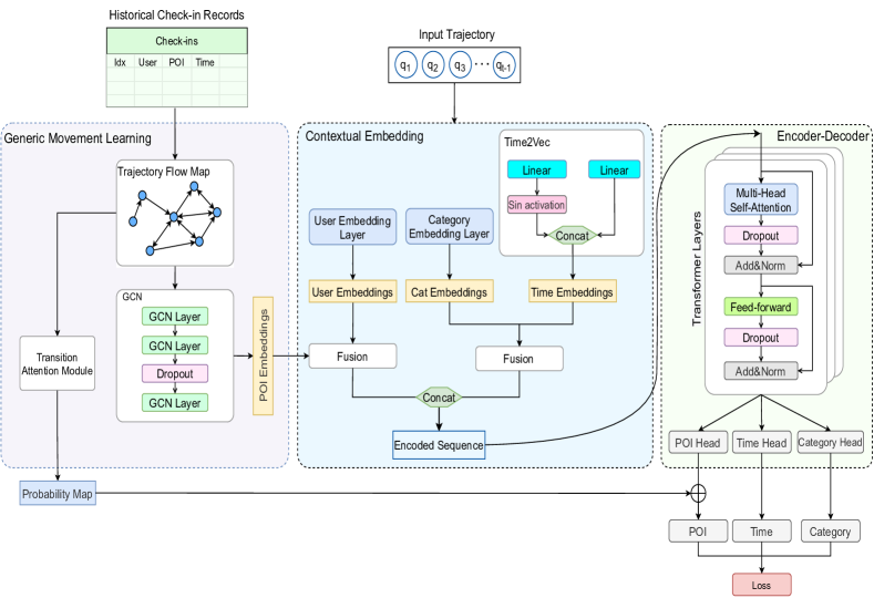
Figure 2. An overview of the proposed GETNext model

Figure 2 illustrates the overall design of our proposed GETNext model. The model fuses several key components. First, we define trajectory flow map which summarizes historical trajectories (see Sec. 4.2). The trajectory flow map influences the recommendation output in two ways:

1. A graph neural network (GNN) is trained on trajectory flow map to produce POI embeddings that encode users’ generic movement patterns on each POI, while incorporating the category, location, and check-in frequency of the POI.

2. An attention module that takes the adjacency matrix of trajectory flow map and node features as input, and produces a transition attention map that explicitly models transition probabilities between POIs.

We then define several contextual modules to obtain user embeddings, POI category embeddings, and time encodings (through a time2vector model) (See Sec. 4.3).

• The user embeddings and the POI embeddings in corresponding trajectories are combined for better personalization.

• The POI category embeddings and the time encodings are also combined to capture users’ temporal preferences of different POI categories (consider, e.g., train stations at peak hours).

The above allows us to produce a single check-in embedding vector by unifying the user, POI category, time stamp, and POI information in a check-in record. Each trajectory can then be encoded as a list of such check-in embeddings. We then employ a transformer encoder and multilayer perceptron (MLP) heads to produce a POI prediction. At last, the predicted POI is adjusted by the learned transition attention map with a residual connection.

4.2. Learning with Trajectory Flow Map

4.2.1. POI Embedding

We observe that different individuals may share certain similar trajectory fragments and the same person can repeat a trajectory multiple times. To utilize these common patterns across historical check-in records, we construct an (user-agnostic) trajectory flow map to provide a global view of users’ generic movements among POI.

Definition 4.0 (Trajectory flow map).

Given the set of historic trajectories $\mathcal{S}=\{S^{i}_{u}\}_{i\in\mathbb{N},u\in U}$, a trajectory flow map is an attributed weighted directed graph $\mathcal{G}=(V,E,\ell,w)$ such that

• the set of nodes is $V=P$ the set of POIs,

• the attribute $\ell(p)$ of each $p\in P$ consists of $(lat,lon,category,freq)$ where $(lat,lon)$ is the coordinate of $p$, $category$ is the category of $p$, and $freq$ is the number of times $p$ occurs in trajectories in $\mathcal{S}$.

• there is an edge from $p_{1}$ to $p_{2}$ if $(p_{1},p_{2})$ appears in a trajectory $S^{i}_{u}$ in $\mathcal{S}$, i.e., they are visited consecutively.

• the weight $w(p_{1},p_{2})$ of any edge $(p_{1},p_{2})$ equals the number of times $(p_{1},p_{2})$ appears in any trajectory in $\mathcal{S}$.

We remark that apart of indicating the movements of users among POIs, the trajectory flow map also implicitly reveals certain spatial proximity between POIs. The intuition is that if two POIs are far from each other, they are less likely to be checked in successively.

Given the trajectory flow map $\mathcal{G}$, our next step is to learn a vectorized representation of POIs that encodes the common POI transition patterns and the attributes of POIs. For this we utilize graph convolution network (GCN). In order to take full advantage of the topological information of $\mathcal{G}$, we use the spectral GCN (Kipf and Welling, 2017). In particular, let $\mathbf{A}\in\mathbb{R}^{N\times N}$ denote the adjacency matrix of $\mathcal{G}$, we first compute the normalized Laplacian matrix as

(1) $$\mathbf{\tilde{L}}=(\mathbf{D}+\mathbf{I}_{N})^{-1}(\mathbf{A}+\mathbf{I}_{N})$$

where $\mathbf{D}$ is the degree matrix and $\mathbf{I}_{N}$ is the identity matrix of $\mathcal{G}$. Next, let $\mathbf{H}^{(0)}=\mathbf{X}\in\mathbb{R}^{N\times C}$ be the input node feature matrix. We define the propagation rule between GCN layers as

(2) $$\mathbf{H}^{(l)}=\sigma\left(\mathbf{\tilde{L}}\mathbf{H}^{(l-1)}\mathbf{W}^{(l)}+b^{(l)}\right)$$

where $\mathbf{H}^{(l-1)}$ denotes the input signals of the $l$-th layer for any $l>0$, $\mathbf{W}^{(l)}\in\mathbb{R}^{C\times\Omega}$ represents the model weights matrix at the $l$-th layer, the corresponding bias $b^{(l)}\in\mathbb{R}^{C\times\Omega}$, and $\sigma$ is a leaky ReLU activation function for non-linearity (with leaky rate 0.2).

From a spatial perspective, at each iteration, the GCN layer updates a node’s embedding by aggregating its neighborhood information together with the node’s own embedding. We stack $l^{*}$ GCN layers to increase the model’s expressiveness. Dropout is employed before the last layer. The output of the GCN module can be written by:

(3) $$\mathbf{e}_{\mathrm{P}}=\mathbf{\tilde{L}}\;\mathbf{H}^{(l^{*})}\mathbf{W}^{(l^{*}+1)}+b^{(l^{*}+1)}\in\mathbb{R}^{N\times\Omega}$$

Finally, the embedding $\mathbf{e}_{p_{i}}$ of POI $p_{i}$ is the $i$-th row of the $N\times\Omega$ matrix $\mathbf{e}_{\mathrm{P}}$. Loosely speaking, the embedding of a POI $p$ indicates the position of $p$ within the historical trajectories of all users and thus captures generic movement patterns at $p$. It will be in turn fed to the transformer downstream to model users’ visiting behaviors. Note that even when the current trajectory is short, the POI embeddings nevertheless provides rich information to the prediction model.

4.2.2. Transition Attention Map

The POI embeddings learned from the graph $\mathcal{G}$ capture generic movement patterns only implicitly. To amplify the impact of the collective signals, we propose a novel transition attention map to explicitly model the transition probabilities from one POI to another. As stated above, these transition probabilities will be used to adjust the final prediction.Given the input node features and $\mathcal{G}$, we compute the attention map $\mathbf{\Phi}$ as:

(4) $$\mathbf{\Phi}_{1}=(\mathbf{X}\times\mathbf{W}_{1})\times\mathbf{a}_{1}\in\mathbb{R}^{N\times 1}$$

(5) $$\mathbf{\Phi}_{2}=(\mathbf{X}\times\mathbf{W}_{2})\times\mathbf{a}_{2}\in\mathbb{R}^{N\times 1}$$

(6) $$\mathbf{\Phi}=(\mathbf{\Phi}_{1}\times\mathbf{1}^{\top}+\mathbf{1}\times\mathbf{\Phi}_{2}^{\top})\odot(\mathbf{\tilde{L}}+J_{N})\in\mathbb{R}^{N\times N}$$

where $\mathbf{W}_{1}$, $\mathbf{W}_{2}\in\mathbb{R}^{C\times h}$ are two trainable feature transformation matrices; $\mathbf{a}_{1}$, $\mathbf{a}_{2}\in\mathbb{R}^{h}$ are two learnable vectors used to construct an $N\times N$ attention matrix by the broadcast add operation; $\mathbf{1}$ is an all-ones vector with shape $\mathbb{R}^{N\times 1}$; $J_{N}$ is the matrix of ones, and $\odot$ stands for element-wise multiplication. We shift the range of the normalized Laplacian matrix $\mathbf{\tilde{L}}$ from $[0,1]$ to $[1,2]$ to avoid zero values.

The $i$-th row of the transition attention map $\mathbf{\Phi}$ indicates the (unnormalized) probability of moving to each POI from the POI $p_{i}$. Given the last POI in the current trajectory, we lookup the transition probabilities stored in the corresponding row of $\mathbf{\Phi}$, and use these probabilities to adjust recommendation results produced by the later transformer module.

4.3. Contextual Embedding Module

Spatio-temporal contexts and user preferences are key factors for personalized next POI recommendations (Feng et al., 2020; Zhao et al., 2020a; Liu et al., 2016b). We proceed to present our contextual embedding module for fusing context information including user embeddings, POI embeddings, POI category embeddings and time encoding.

4.3.1. POI-User Embeddings Fusion

The POI embeddings are learned from the trajectory flow map and omit user-specific patterns. To capture a specific user $u$’s general behaviors, we train an embedding layer that project each user to a low-dimensional vector. The embedding of each user is learned from his/her historical check-in sequences. Formally, the user embedding of $u$ is

(7) $$\mathbf{e}_{u}=f_{\text{embed}}(u)\in\mathbb{R}^{\Omega}.$$

In order to construct the representation of each check-in activity, a straightforward solution is to concatenate the POI embedding and user embedding. We feed the concatenated vector into a dense layer to fine-tune the fused embedding and increase its representational power. The output can be denoted as

(8) $$\mathbf{e}_{p,u}=\sigma(\mathbf{w}_{p,u}[\mathbf{e}_{p};\mathbf{e}_{u}]+b_{p,u})\in\mathbb{R}^{\Omega\times 2},$$

where $\mathbf{w}_{p,u}$ and $b_{p,u}$ are weights vector and the bias, respectively, and $[\cdot;\cdot]$ represents the concatenation. The dimension of the output embedding is twice as large as the POI embedding or user embedding. In other words, the size of embedding vector remains unchanged after the fusion.

4.3.2. Time-Category Embeddings Fusion

The visiting behaviors of users are naturally time-dependent. For example, Fig. 3 shows the check-in frequencies of two POI categories in a day. “Train station” has two clear peaks during the rush hours (around 8AM and 6PM). On the contrary, “bars” shows a diametrically opposite pattern where most check-in activities happen after 6PM. Such observations motivate us to consider temporal patterns of POI categories for next POI recommendation. For example, a train station – rather than a bar – should be recommended at 8AM.

It is worth noting that check-ins at individual POIs may also exhibit certain temporal patterns. However, because of scarcity of check-ins and noise in data, the temporal patterns of individual POIs are far less clear and stable as those of categories. Take NYC dataset as an example, which contains 227k check-in records, 38k POIs, and 400 categories. On average, each POI only gets less than 6 check-ins. The check-ins at the category level, in contrast, is more than 570 per category. We thus explore the temporal patterns of POI categories instead of individual POIs.

(a) “Train station”

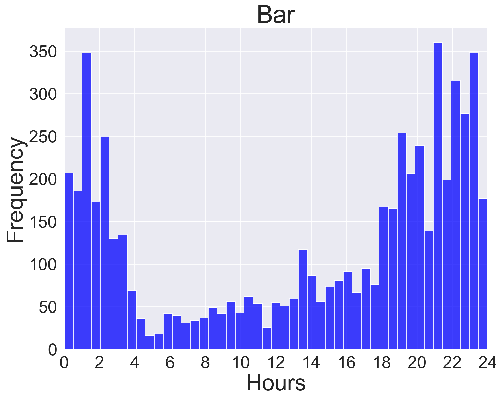
(b) “Bar”

Figure 3. Average hourly check-in frequency of two POI categories (“train station” and “bar”) in NYC dataset

Similar to the POI-User embedding fusion module, we first encode POI category and time. We adopt time2vector, a state-of-the-art time encoding model (Kazemi et al., 2019). Specifically, we divide the 24 hours in a day to 48 slots with 30 minutes per slot. We project a (scalar) time value to one of the time slots. The embedding of a time slot $t$, denoted as $\mathbf{e}_{t}$, is a vector of length $k+1$. The $i$-th element is defined as:

(9) $$\mathbf{e}_{t}[i]=\begin{cases}\omega_{i}t+\varphi_{i},&\text{ if }i=0.\\ \sin\left(\omega_{i}t+\varphi_{i}\right),&\text{ if }1\leq i\leq k.\end{cases}$$

where $\omega$ and $\varphi$ are learnable parameters. The $\sin$ activation function is used to capture periodic patterns.

We employ another embedding layer for POI categories. The embedding of a category $c$ is

(10) $$\mathbf{e}_{c}=f_{\text{embed}}(c)\in\mathbb{R}^{\Psi},$$

where $\Psi$ is the embedding dimension.

Next, we fuse the time embedding $\mathbf{e}_{t}$ and category embedding $\mathbf{e}_{c}$ to form a single category-time representation by a dense layer:

(11) $$\mathbf{e}_{c,t}=\sigma(\mathbf{w}_{c,t}[\mathbf{e}_{t};\mathbf{e}_{c}]+b_{c,t})\in\mathbb{R}^{\Psi\times 2},$$

where $\mathbf{w}_{c,t}$ is a learnable weight vector and $b_{c,t}$ is the bias.

Finally, the embedding of a check-in $q=\langle p,u,t\rangle$ where POI $p$ has category $c$ is the concatenation $\mathbf{e}_{q}=[\mathbf{e}_{p,u};\mathbf{e}_{c,t}]$. As a result, each input trajectory $(q_{1},\ldots,q_{s})$ is represented by a list of check-in embeddings $(\mathbf{e}_{q_{1}},\ldots,\mathbf{e}_{q_{s}})$. We will feed the encoded sequence to the transformer encoder.

4.4. Transformer Encoder and MLP Decoders

4.4.1. Transformer Encoder

The transformer is a purely attention based encoder-decoder network, which was firstly proposed by Vaswani et al (Vaswani et al., 2017) in 2017. Due to its distinguished computational efficiency and outstanding performance compared with traditional models, transformers has become the paradigm-of-choice in NLP, and more recently in image recognition (Dosovitskiy et al., 2020), video understanding (Neimark et al., 2021), time series analysis (Lim et al., 2021).

We adopt transformer for next-POI recommendation as it is a natural sequence prediction task. Since the goal is to predict only the next immediate POI given a check-in sequence, we adopt the transformer encoder only followed by several MLP heads (without the transformer decoder). For the encoder, we stack several standard transformer encoder layers with positional encoding. Each layer consists of a multi-head self-attention module followed by a position-wise fully-connected network. Residual connections and normalization are applied to both modules.

Formally, given an input trajectory $S_{u}=(q_{u}^{1},q_{u}^{2},\dots,q_{u}^{k})$, to predict the POI in the next check-in activity $q_{u}^{k+1}$, we firstly take the check-in embedding of each historical check-in $q_{u}^{i}$, $1\leq i\leq k$, as defined in Sec 4.3. We then stack these check-in embeddings to form an input tensor of the first encoder layer, which can be denoted as $\mathcal{X}^{[0]}\in\mathbb{R}^{k\times d}$, where $d$ represents the embedding dimension of each check-in record. Particularly, $d$ equals to the length of $\mathbf{e}_{q}$, i.e., $d=2\times(\Omega+\Psi)$. It is worth noting that the embedding length $d$ remains unchanged across all encoder layers to facilitate residual connections and layers stacking. In other words, ignoring padding, the output shape of the encoder layer $l$ coincide with the input shape, i.e., $\mathcal{X}^{[l+1]}\in\mathbb{R}^{k\times d}$.

For layer $l$, the input $\mathcal{X}^{[l]}\in\mathbb{R}^{k\times d}$ is firstly transformed by a multi-head self-attention module (the number of heads is 2 in our experiments). For the first attention head, the output is:

(12) $$\boldsymbol{S}=\mathcal{X}^{[l]}\boldsymbol{W}_{q}(\mathcal{X}^{[l]}\boldsymbol{W}_{k})^{T}\in\mathbb{R}^{k\times k}$$

(13) $$\boldsymbol{S}^{\prime}_{i,j}=\frac{\exp\left(\boldsymbol{S}_{i,j}\right)}{\sum_{j=1}^{d}\exp\left(\boldsymbol{S}_{i,j}\right)}$$

(14) $$\operatorname{head}_{1}=\boldsymbol{S}^{{\prime}}\mathcal{X}^{[l]}\boldsymbol{W}_{v}\in\mathbb{R}^{k\times d/h},$$

where $\boldsymbol{W}_{q}\in\mathbb{R}^{d\times d/h}$, $\boldsymbol{W}_{k}\in\mathbb{R}^{d\times d/h}$ and $\boldsymbol{W}_{v}\in\mathbb{R}^{d\times d/h}$ are learnable weight matrices corresponding to “query”, “key” and “value”, respectively. Here we ignore the bias in equations. The dot product attention, i.e., $\boldsymbol{S}_{i,j}$ indicates the correlations between the $i$-th and $j$-th check-in activities. Next, softmax function is applied to assure the attention weights sum to one. After projecting the input data to an output feature space by $\boldsymbol{W}_{v}$, we use the learned attention matrix to adjust the contribution of each check-in record. Last, we stack different attention heads and employ another linear transformation $\boldsymbol{W}_{o}\in\mathbb{R}^{d\times d}$ to merge the representations from different attention spaces:

(15) $$\operatorname{Multihead}(\mathcal{X}^{[l]})=[\operatorname{head}_{1};\cdots;\operatorname{head}_{h}]\times\boldsymbol{W}_{o}\in\mathbb{R}^{k\times d}.$$

Furthermore, the layer norm and residual connection is applied to the attention module. Therefore, the final output of the attention module can be written as

(16) $$\mathcal{X}^{[l]}_{\text{attn}}=\operatorname{LayerNorm}\left(\mathcal{X}^{[l]}+\operatorname{Multihead}(\mathcal{X}^{[l]})\right).$$

In each encoder layer, a fully-connected (FC) network is attached after the attention model. Denote the output of multihead attention module as $\mathcal{X}^{[l]}_{\text{attn}}$. The FC network can be represented as

(17) $$\mathcal{X}^{[l]}_{\text{FC}}=\operatorname{ReLU}(\mathbf{W}_{1}\mathcal{X}^{[l]}_{\text{attn}}+b_{1})\mathbf{W}_{2}+b_{2}\in\mathbb{R}^{k\times d},$$

where $\mathbf{W}_{1}$, $\mathbf{W}_{2}$ are trainable weight matrices and $b_{1}$, $b_{2}$ are biases. Similarly, the output of the $l$-th encoder layer is

(18) $$\mathcal{X}^{[l+1]}=\operatorname{LayerNorm}(\mathcal{X}^{[l]}_{\text{attn}}+\mathcal{X}^{[l]}_{\text{FC}})\in\mathbb{R}^{k\times d}.$$

4.4.2. MLP Decoders

The transformer encoder layers distill the useful information from the input trajectory check-in embeddings to a feature space. In order to predict the user’s next move, we replace the transformer decoder with several multi-layer perceptron (MLP) decoders. In particular, we employ three MLP heads to predict the next POI, visit time, and POI category, respectively. Denote the output of the encoder as $\mathcal{X}^{[l^{*}]}$, the MLP heads can be written by

(19) $$\mathbf{\hat{Y}}_{\text{poi}}=\mathcal{X}^{[l^{*}]}\mathbf{W}_{\text{poi}}+b_{\text{poi}}$$

(20) $$\mathbf{\hat{Y}}_{\text{time}}=\mathcal{X}^{[l^{*}]}\mathbf{W}_{\text{time}}+b_{\text{time}}$$

(21) $$\mathbf{\hat{Y}}_{\text{cat}}=\mathcal{X}^{[l^{*}]}\mathbf{W}_{\text{cat}}+b_{\text{cat}}$$

where $\mathbf{W}_{\text{poi}}\in\mathbb{R}^{d\times N}$, $\mathbf{W}_{\text{time}}\in\mathbb{R}^{d\times 1}$, $\mathbf{W}_{\text{cat}}\in\mathbb{R}^{d\times\Gamma}$ are weights in MLP, and $\Gamma$ represents the number of POI categories. For the output of POI head $\mathbf{\hat{Y}}_{\text{poi}}\in\mathbb{R}^{k\times N}$, we only concern about the last row which corresponds to the POI recommendation for the future move. We in addition combine this POI recommendation with the transition attention map defined in Sec. 4.2.2. The final recommendation is

(22) $$\mathbf{\hat{y}}_{\text{poi}}=\mathbf{\hat{Y}}_{\text{poi}}^{(k\cdot)}+\Phi^{(p_{k}\cdot)}\in\mathbb{R}^{1\times N},$$

where $\mathbf{\hat{Y}}_{\text{poi}}^{(k\cdot)}$ represents the $k$-th row of $\mathbf{\hat{Y}}_{poi}$ and $\Phi^{(p_{k}\cdot)}$ is the $p_{k}$-th row of transition map $\Phi$, $p_{k}$ stands for the POI of check-in $q_{u}^{k}$.

As shown above, besides the POI head, we also add the time head and category head. The main reason we predict the next check-in time along with POI is the following: The time gaps between two check-ins fluctuate considerably (e.g., between half an hour to as long as 6 hours). This is reasonable as users spend unequal lengths of time in different POIs or forget to record certain check-ins. However, such fluctuation has a considerable impact to prediction. Indeed, a user should receive different recommendations at 5PM for the next hour and for the next 5 hours. We therefore recommend the next POI as well as the next check-in time, and use the time head as a calibration of the time modeling. Moreover, the category head is employed to regulate next POI prediction as forecasting the next POI category is easier than exact POI prediction.

4.4.3. Loss

All MLP heads in the decoder are taken into the consideration for training where outputs from the time and category heads act as regularization terms. In other words, we calculate a weighted sum of the losses of all MLP heads. Cross entropy is used as the loss function for POI and POI category prediction. The mean squared error (MSE) is used for the performance of time prediction. Moreover, since we normalized the in-day 24 hours to [0, 1], the scale of time loss is significantly smaller than the other two. To balance the magnitude of gradients with other losses, the time loss term is amplified 10-fold, i.e., the final loss is

(23) $$\mathcal{L}_{\text{final}}=\mathcal{L}_{\text{poi}}+10\times\mathcal{L}_{\text{time}}+\mathcal{L}_{\text{cat}}.$$

5. Experiments

In this section, we evaluate our proposed model on real-world datasets.

5.1. Experimental Setup

5.1.1. Datasets

We conduct experiments on three public datasets collected from location-based service platforms: FourSquare-NYC (Yang et al., 2014), FourSquare-TKY (Yang et al., 2014), and Gowalla-CA (Yuan et al., 2013). FourSquare-NYC was collected from Apr. 2012 to Feb. 2013 in New York City, and FourSquare-TKY from Tokyo during the same time period. Gowalla-CA consists of check-ins between Feb. 2009 and Oct. 2010 within California and Nevada from Gowalla (Yuan et al., 2013). Each record contains user, POI, POI category, GPS coordinates, and timestamp. For all three datasets, we exclude unpopular POIs that have less than 10 check-in records, and also filter out users with fewer than 10 check-in history. Next, users’ entire check-in sequence were broken into trajectories with 24-hour intervals. In rare cases, the trajectory contains only a single check-in; these cases are eliminated from the dataset. Next we split the dataset into train/validation/test sets in chronological order. The first 80% check-ins are the training set and used to build the trajectory flow map $\mathcal{G}$, the middle 10% are validation set and the remaining 10% form the test set. Had user or POI not appeared in training but emerged in test, we skip that user or POI when measuring the prediction performance. Key statistics of datasets are shown in Table 1.

Table 1. Dataset statistics

	#user	#poi	#cat	#checkin	#trajectory
NYC	1,075	5,099	318	104,074	14,160
TKY	2,281	7,844	291	361,430	44,692
CA	4,318	9,923	301	250,780	32,920

5.1.2. Evaluation metrics

We compute the accuracy@$k$ (Acc@$k$) and mean reciprocal rank (MRR), which are common metrics in recommender systems. Accuracy@$k$ indicates whether the true POI appears in the top-$k$ recommended POIs. As acc@$k$ views the top-$k$ recommendations as an unordered list while ignoring the ordering of the correct prediction, we employed MRR which measures the index of the correctly recommended POI in the ordered result list. Given a dataset with $m$ samples (trajectories), define

$$\text{Acc}@k=\frac{1}{m}\sum_{i=1}^{m}\mathbbm{1}(rank\leq k)$$

$$\text{MRR}=\frac{1}{m}\sum_{i=1}^{m}\frac{1}{rank}$$

where $\mathbbm{1}$ is the indicator function. It returns 1 if the condition is true, otherwise 0. Rank represents the rank of the true next POI in the recommended ordered list. In general, for all these metrics, the larger the value, the better the performance.

5.1.3. Baselines

We adopt the following baselines.

• MF (Koren et al., 2009) is a classical methods in many recommendation problems. It learned the latent representation of users and POIs by Matrix Factorization.

• FPMC (Rendle et al., 2010) combined Matrix Factorization and Markov Chain together to model both user long-term preference and sequential behavior.

• LSTM (Hochreiter and Schmidhuber, 1997) is a variant of RNN model to handle sequential data. Compared with standard RNN model, LSTM models both short-term and long-term sequential patterns.

• PRME (Feng et al., 2015) proposed a pair-wise embedding method named personalized ranking metric embedding to capture the user preference and sequential transition between POIs.

• ST-RNN (Liu et al., 2016b) adopted the time, distance transition matrix to model the local temporal and spatial contexts in additional to a RNN for user’s sequential patterns capturing.

• STGN (Zhao et al., 2020a) extends the conventional LSTM by adding spatial gates and temporal gates to capture user’s preference in space and time dimension.

• STGCN (Zhao et al., 2020a) is an updated version of STGN which used coupled input and forget gates.

• PLSPL (Wu et al., 2020) learned user’s long term taste by attention mechanism and short term preference with LSTM, and combined them by personalized linear layers.

• STAN (Luo et al., 2021) utilizes the spatiotemporal information of checkins along the trajectory with self-attention layers to capture the point-to-point interaction between non-adjacent check-ins.

5.1.4. Experiment Settings

We developed our model using the PyTorch framework and conducted experiments on the following hardware platform (CPU: AMD Ryzen 9 5900X, GPU: NVIDIA GeForce RTX 3090). The key hyper-parameter settings in our model are listed below. The embedding dimensions of POI and user are both $\Omega=128$. The time, POI category embedding length are $\Psi=32$. The GCN model has three hidden layers with 32, 64, 128 channels each. The transition attention module convert the input node features to the 128-dim vector. For transformer, we stacked two encoder layers. The dimensions of the feed-forward network in the transformer encoder layer is 1024, and two attention heads are used in the multi-headed attention module. Moreover, we employed the Adam optimizer with 1e-3 learning rate and 5e-4 weight decay rate. Dropout are enabled in both GCN model and Transformer encoder with rate 0.3. Another important parameter is the weight of time loss $\alpha$ where we set to 10 to match the scale of POI loss and category loss. We use the same settings in three datasets and run each model 200 epochs with batch size 20.

Table 2. Performance comparison in Acc@k and MRR on three datasets

	NYC					TKY					CA
	Acc@1	Acc@5	Acc@10	Acc@20	MRR	Acc@1	Acc@5	Acc@10	Acc@20	MRR	Acc@1	Acc@5	Acc@10	Acc@20	MRR
MF	0.0368	0.0961	0.1522	0.2375	0.0672	0.0241	0.0701	0.1267	0.1845	0.4861	0.0110	0.0442	0.0723	0.1190	0.0342
FPMC	0.1003	0.2126	0.2970	0.3323	0.1701	0.0814	0.2045	0.2746	0.3450	0.1344	0.0383	0.0702	0.1159	0.1682	0.0911
LSTM	0.1305	0.2719	0.3283	0.3568	0.1857	0.1335	0.2728	0.3277	0.3598	0.1834	0.0665	0.1306	0.1784	0.2211	0.1201
PRME	0.1159	0.2236	0.3105	0.3643	0.1712	0.1052	0.2278	0.2944	0.3560	0.1786	0.0521	0.1034	0.1425	0.1954	0.1002
ST-RNN	0.1483	0.2923	0.3622	0.4502	0.2198	0.1409	0.3022	0.3577	0.4753	0.2212	0.0799	0.1423	0.1940	0.2477	0.1429
STGN	0.1716	0.3381	0.4122	0.5017	0.2598	0.1689	0.3391	0.3848	0.4514	0.2422	0.0810	0.1842	0.2579	0.3095	0.1675
STGCN	0.1799	0.3425	0.4279	0.5214	0.2788	0.1716	0.3453	0.3927	0.4763	0.2504	0.0961	0.2097	0.2613	0.3245	0.1712
PLSPL	0.1917	0.3678	0.4523	0.5370	0.2806	0.1889	0.3523	0.4150	0.4880	0.2542	0.1072	0.2278	0.2995	0.3401	0.1847
STAN	0.2231	0.4582	0.5734	0.6328	0.3253	0.1963	0.3798	0.4464	0.5119	0.2852	0.1104	0.2348	0.3018	0.3502	0.1869
Ours	0.2435	0.5089	0.6143	0.6880	0.3621	0.2254	0.4417	0.5287	0.5829	0.3262	0.1357	0.2852	0.3590	0.4241	0.2103

5.2. Results

Table 2 shows the performance comparison between our model and the baselines on three datasets. We report the top-1, top-5, top-10, top-20 accuracy and MRR. Generally speaking, all models perform better on NYC and TKY datasets than CA. The main reason is POIs in NYC and TKY are constrained inside a relatively small area (New York city and Tokyo city). But POIs in CA datasets spread across California and Nevada, result in a sparser dataset.

For all datasets, our model outperforms the baselines by large margins. For example, in NYC dataset, we achieve 24.35% top-1 accuracy while the best baseline STAN is 22.31%. On top-5 accuracy, our model gains about 11% improvement compared with baselines, and on top-20 accuracy, a 8.7% performance increase is recorded. Similar results are shown in TKY. Moreover, state-of-the-art attend-based or LSTM-based recommendation models such as STAN, PLSPL, STGCN perform significantly better than traditional Markov-chain based or Matrix factorization based models like FPMC, PRME. For example, the top-1 accuracy of STAN is twice as much as FPMC, namely 22.31% to 10.03% on NYC.

CA dataset contains 9.9k POIs and 250k check-in records widely spread in an area over 400,000 $km^{2}$ where the TKY dataset contains 7.8k POIs with 361k check-ins squeezed in about 2,000 $km^{2}$. Because of the more seriously data scarcity problem in both the number of checkins and spatial sparsity of POIs, models usually cannot reach the same level of performance in CA as they are in NYC and TKY. More specifically, the top-1 accuracy of STAN on NYC is 22.31% which drops to 11.04% on CA. Similar patterns appear on our model as well. The top-1 accuracy of our model on CA is 13.57%, which beats all baselines but much lower than it on NYC dataset.

5.3. Inspecting the Trajectory Flow Map

Previous section demonstrates the overall performance of the proposed framework. In this section, we elaborate on the advantages of the trajectory flow map. We show that our method mitigates the cold-start problem for inactive users and short trajectories compared with other methods. Then we remove the trajectory flow map and compare the performance by learning POI embeddings via embedding layers. At last, we describe the quantitative features of the graph built for NYC dataset.

5.3.1. Inactive users and active users

Given a dataset, after splitting it into train, validation, and test, we count the number of trajectories of each user in the train set only. We then mark the top 15% as the most active users, the bottom 15% as inactive users, and the rest are normal users. Next, we evaluate the model on the test set and record the performance of different user groups.

Take NYC dataset as an example. Out of 1,047 users in the training set, we identify 137 inactive users with less than 13 trajectories; 144 most active users with more than 41 trajectories, and 766 normal users. In general, inactive users do not have rich historical information making it hard to learn from the data. To mitigate this challenge, we built the global trajectory flow map and try to improve the recommendation results of inactive users by leveraging other users’ sequences.

The performance in different user groups of our model and the baseline is shown in Table 3. Compared with the baseline model, our model achieves higher accuracy in all three user groups. For inactive users, the top-1 and top-10 accuracy of our model is 12.24% and 43.94% while corresponding accuracy of STGN is 9.06% and 31.24%. A huge improvement is also observed on top-5 accuracy and top-20 accuracy.

Table 3. Cold Start (due to inactive users) performance on NYC

User Groups	Model	Acc@1	Acc@5	Acc@10	Acc@20
Inactive	STGN	0.0926	0.2435	0.3124	0.3763
Normal	STGN	0.1778	0.3576	0.4189	0.5125
Very active	STGN	0.1813	0.3832	0.4274	0.5398
Inactive	Ours	0.1224	0.3471	0.4394	0.4529
Normal	Ours	0.2421	0.4739	0.5422	0.6430
Very active	Ours	0.2692	0.5639	0.6995	0.7762

5.3.2. Short trajectories and long trajectories

Short trajectories present another challenge in next POI recommendation. The lack of information in a short-trajectory is reflected in its limited spatio-temporal contexts, especially when the number of known check-ins in a trajectory is merely one or two. We define the short trajectory dynamically according to the dataset. In particular, we order trajectories in the test sets by length and label the top 15% as long trajectories and bottom 15% as short ones.

Table 4 shows the performance of our mdoel and STGN on three trajectory groups of NYC dataset. Our model does not show significant difference on recommendation performance between the short trajectory and long trajectory. For example, the top-1 accuracy is 21.86% and 24.52% on short and long trajectories, and the top-20 accuracy of short trajectories is 57.82%. However, STGN, an extended LSTM model, is quite sensitive to trajectory length and perform unsatisfying on short trajectories with 7.23% top-1 accuracy and 33.28% top-20 accuracy.

Table 4. Cold Start (due to short trajectory) performance on NYC

Trajectory	Model	Acc@1	Acc@5	Acc@10	Acc@20
Short trajs	STGN	0.0723	0.2117	0.2784	0.3328
Middle trajs	STGN	0.1921	0.3471	0.4397	0.5231
Long trajs	STGN	0.1934	0.3516	0.4380	0.5322
Short trajs	Ours	0.2186	0.4561	0.5269	0.5782
Middle trajs	Ours	0.2441	0.4927	0.5881	0.6519
Long trajs	Ours	0.2452	0.5378	0.6698	0.7681

5.3.3. Removing trajectory flow map

For comparison, we remove the trajectory flow map from our model and learn the POI representations by embedding layers to show the contributions of the global trajectory flow map . Table 5 shows the performance of model without trajectory flow map on three user groups and three trajectory groups. Summarizing Tables 3, 4 and 5, we observe that after removing trajectory flow map , the top-10 accuracy of inactive users drops from 42.11% to 34.70%, and performance drops from 52.06% to 47.21% for short trajectories. These experiments verify that global trajectory flow map benefits the top-$k$ accuracy of inactive users and short trajectories when $k$ is large. However, for cold start problem, the top-1 accuracy do not gain much improvement from trajectory flow map . This phenomenon aligns to our assumption that incorporating generic movement patterns most help with top-$k$ accuracy for sufficiently large $k$. Thus, even the top-1 accuracy does not show much difference, the top-10 performance is indeed better.

Table 5. Performance of proposed model without trajectory flow map on NYC

	Model	Acc@1	Acc@5	Acc@10
Inactive users	Ours w/o graph	0.1105	0.2983	0.3470
Normal users	Ours w/o graph	0.2094	0.4228	0.5010
Very active users	Ours w/o graph	0.2488	0.5271	0.6815
Short trajs	Ours w/o graph	0.1914	0.4059	0.4721
Middle trajs	Ours w/o graph	0.2129	0.4490	0.5232
Long trajs	Ours w/o graph	0.2012	0.4882	0.6186

5.3.4. Analysis of the trajectory flow map

We analyze structural properties of the trajectory flow map $\mathcal{G}$ constructed for NYC dataset as a case study. The constructed graph contains 4980 nodes and 37,756 edges. The average in-degree and out-degree are both 7.58. In a macroscopic perspective, there are about 7.58 possible choices for the next move in general. The mean edge weight is 1.91. That is to say if POI A and POI B are in two successive check-ins, then the average number of this check-in order is 1.91. Also, the average clustering coefficient of this graph is 0.1866, suggesting significant clustering. Figure 4 shows the partial graph of NYC dataset (without edge weight nor direction). The illustration demonstrates that the graph contains non-trivial structural information to be explored. In particular, the graph contains several visible communities, yet there are also many long paths suggesting that the graph deviates from a typical small-world network.

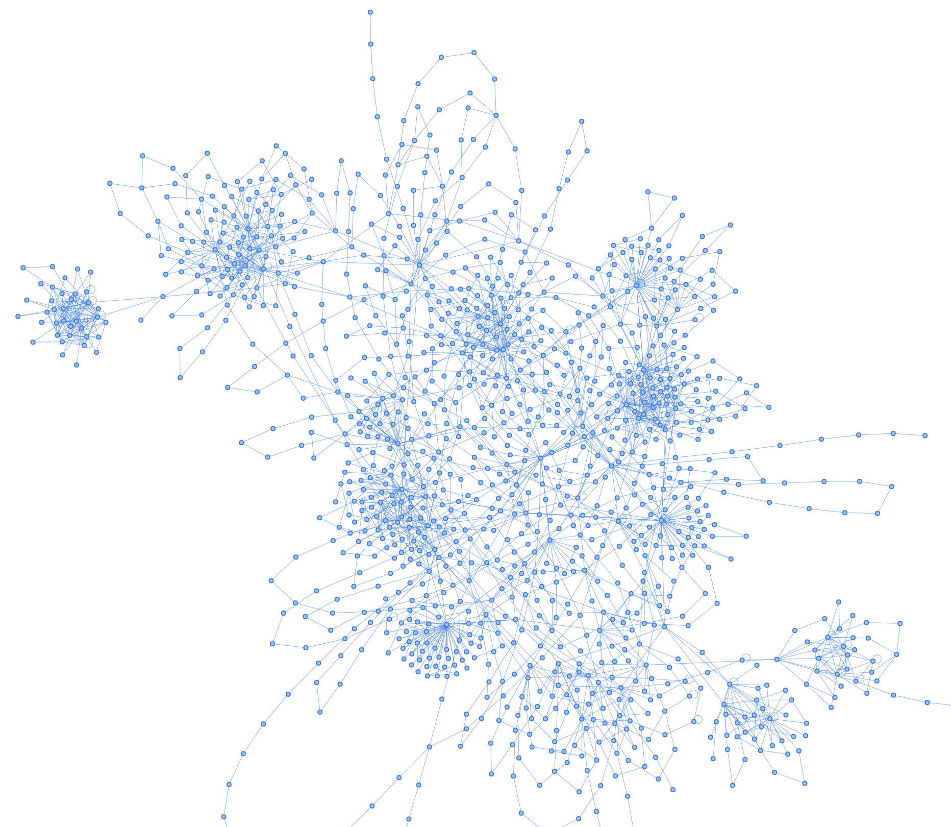
Figure 4. Partial trajectory flow map of NYC (directions and edge weights are removed for better visualization)

5.4. Ablation Study

We conduct an ablation study to evaluate the impact of each proposed component to the model’s final performance on NYC dataset. Particularly, seven experiments are conducted: 1) the full model; 2) without trajectory flow map and learn POI embeddings by embedding layers; 3) without transformer encoder and sequential data are handled by LSTM; 4) without time and category information; 5) without GCN and the random walk were employed to learn node embeddings from transtion graph; 6) instead of fusing user and POI embeddings, we concatenate them directly; 7) without time decoder and category decoder. In each experiment, rest settings remain unchanged as in the full model and only one component is either replaced or removed. The results are shown in Table 6.

Table 6. Ablation study: Comparing the full model with 6 variants

	Acc@1	Acc@5	Acc@10	Acc@20	MRR
Full Model	0.2435	0.5089	0.6143	0.6880	0.3621
w/o Graph	0.2163	0.4512	0.5248	0.6402	0.3398
w/o Transformer	0.2221	0.4617	0.5520	0.6261	0.3317
w/o Time&Cat	0.2296	0.4804	0.5489	0.6484	0.3495
w/o GCN	0.2062	0.4582	0.5601	0.6589	0.3187
w/o Fusion	0.2355	0.4731	0.5726	0.6614	0.3533
Single decoder	0.2207	0.4721	0.5722	0.6591	0.3443

The full model achieves the best performance. For the rest components, the results suggest that trajectory flow map and GCN play a bigger role than other components in the overall performance. For example, top-1 accuracy drops from 24.35% to 21.63% and 20.62% without trajectory flow map or using random walk to learn POI embeddings. Other components also contribute to the final recommendation results. For instance, the transformer can leverage the useful information from historical data automatically by the self-attention module, with less parameters to train and better performance.

6. Conclusion

In this paper, we propose GETNext, the first next POI recommendation model that utilizes graph-based learning on a global graph structure. In particular, we introduce trajectory flow map to capture generic movement patterns of the users to address the inactive user and short trajectory issues. We defined sophisticated embeddings to encode spatio-temporal contexts, which include user-POI as well as time-category embeddings. We feed all embeddings into a transformer model, whose output is further enhanced through a transition attention map. Through a series of experiments on three real-world datasets, we demonstrate that our model significantly outperform all current state-of-the-art models by a large margin, and verify the benefits of the different components of our model. For future work, we will further explore and distinguish the temporal patterns, e.g., between work-days and weekends. Another future work is to classify users by their behaviors and build trajectory flow map for each type of users.

Acknowledgement. This research is supported by the Marsden Fund Council from Government funding (MFP-UOA2123), administered by the Royal Society of New Zealand.

References

- (1)
- Chang et al. (2020) Buru Chang, Gwanghoon Jang, Seoyoon Kim, and Jaewoo Kang. 2020. Learning graph-based geographical latent representation for point-of-interest recommendation. In Proceedings of the 29th ACM International Conference on Information & Knowledge Management. 135–144.
- Cheng et al. (2013) Chen Cheng, Haiqin Yang, Michael R Lyu, and Irwin King. 2013. Where you like to go next: Successive point-of-interest recommendation. In Twenty-Third international joint conference on Artificial Intelligence.
- Dosovitskiy et al. (2020) Alexey Dosovitskiy, Lucas Beyer, Alexander Kolesnikov, Dirk Weissenborn, Xiaohua Zhai, Thomas Unterthiner, Mostafa Dehghani, Matthias Minderer, Georg Heigold, Sylvain Gelly, et al. 2020. An image is worth 16x16 words: Transformers for image recognition at scale. arXiv preprint arXiv:2010.11929 (2020).
- Feng et al. (2018) Jie Feng, Yong Li, Chao Zhang, Funing Sun, Fanchao Meng, Ang Guo, and Depeng Jin. 2018. Deepmove: Predicting human mobility with attentional recurrent networks. In Proceedings of the 2018 world wide web conference. 1459–1468.
- Feng et al. (2015) Shanshan Feng, Xutao Li, Yifeng Zeng, Gao Cong, Yeow Meng Chee, and Quan Yuan. 2015. Personalized ranking metric embedding for next new poi recommendation. In Twenty-Fourth International Joint Conference on Artificial Intelligence.
- Feng et al. (2020) Shanshan Feng, Lucas Vinh Tran, Gao Cong, Lisi Chen, Jing Li, and Fan Li. 2020. Hme: A hyperbolic metric embedding approach for next-poi recommendation. In Proceedings of the 43rd International ACM SIGIR Conference on Research and Development in Information Retrieval. 1429–1438.
- Hochreiter and Schmidhuber (1997) Sepp Hochreiter and Jürgen Schmidhuber. 1997. Long short-term memory. Neural computation 9, 8 (1997), 1735–1780.
- Jiang et al. (2015) Shuhui Jiang, Xueming Qian, Jialie Shen, Yun Fu, and Tao Mei. 2015. Author topic model-based collaborative filtering for personalized POI recommendations. IEEE transactions on multimedia 17, 6 (2015), 907–918.
- Kazemi et al. (2019) Seyed Mehran Kazemi, Rishab Goel, Sepehr Eghbali, Janahan Ramanan, Jaspreet Sahota, Sanjay Thakur, Stella Wu, Cathal Smyth, Pascal Poupart, and Marcus Brubaker. 2019. Time2vec: Learning a vector representation of time. arXiv preprint arXiv:1907.05321 (2019).
- Kipf and Welling (2017) Thomas N Kipf and Max Welling. 2017. Semi-supervised classification with graph convolutional networks. (2017).
- Koren et al. (2009) Yehuda Koren, Robert Bell, and Chris Volinsky. 2009. Matrix factorization techniques for recommender systems. Computer 42, 8 (2009), 30–37.
- Li et al. (2021) Yang Li, Tong Chen, Hongzhi Yin, and Zi Huang. 2021. Discovering collaborative signals for next POI recommendation with iterative Seq2Graph augmentation. In IJCAI.
- Lim et al. (2021) Bryan Lim, Sercan Ö Arık, Nicolas Loeff, and Tomas Pfister. 2021. Temporal fusion transformers for interpretable multi-horizon time series forecasting. International Journal of Forecasting (2021).
- Liu et al. (2016b) Qiang Liu, Shu Wu, Liang Wang, and Tieniu Tan. 2016b. Predicting the next location: A recurrent model with spatial and temporal contexts. In Thirtieth AAAI conference on artificial intelligence.
- Liu et al. (2016a) Yanchi Liu, Chuanren Liu, Bin Liu, Meng Qu, and Hui Xiong. 2016a. Unified point-of-interest recommendation with temporal interval assessment. In Proceedings of the 22nd ACM SIGKDD international conference on knowledge discovery and data mining. 1015–1024.
- Luo et al. (2021) Yingtao Luo, Qiang Liu, and Zhaocheng Liu. 2021. Stan: Spatio-temporal attention network for next location recommendation. In Proceedings of the Web Conference 2021. 2177–2185.
- Neimark et al. (2021) Daniel Neimark, Omri Bar, Maya Zohar, and Dotan Asselmann. 2021. Video transformer network. arXiv preprint arXiv:2102.00719 (2021).
- Rendle et al. (2010) Steffen Rendle, Christoph Freudenthaler, and Lars Schmidt-Thieme. 2010. Factorizing personalized markov chains for next-basket recommendation. In Proceedings of the 19th international conference on World wide web. 811–820.
- Sun et al. (2020) Ke Sun, Tieyun Qian, Tong Chen, Yile Liang, Quoc Viet Hung Nguyen, and Hongzhi Yin. 2020. Where to go next: Modeling long-and short-term user preferences for point-of-interest recommendation. In Proceedings of the AAAI Conference on Artificial Intelligence, Vol. 34. 214–221.
- Tang et al. (2015) Jian Tang, Meng Qu, Mingzhe Wang, Ming Zhang, Jun Yan, and Qiaozhu Mei. 2015. Line: Large-scale information network embedding. In Proceedings of the 24th international conference on world wide web. 1067–1077.
- Vaswani et al. (2017) Ashish Vaswani, Noam Shazeer, Niki Parmar, Jakob Uszkoreit, Llion Jones, Aidan N Gomez, Łukasz Kaiser, and Illia Polosukhin. 2017. Attention is all you need. In Advances in neural information processing systems. 5998–6008.
- Wu et al. (2019) Yuxia Wu, Ke Li, Guoshuai Zhao, and Xueming Qian. 2019. Long-and short-term preference learning for next POI recommendation. In Proceedings of the 28th ACM international conference on information and knowledge management. 2301–2304.
- Wu et al. (2020) Yuxia Wu, Ke Li, Guoshuai Zhao, and QIAN Xueming. 2020. Personalized long-and short-term preference learning for next POI recommendation. IEEE Transactions on Knowledge and Data Engineering (2020).
- Xie et al. (2016) Min Xie, Hongzhi Yin, Hao Wang, Fanjiang Xu, Weitong Chen, and Sen Wang. 2016. Learning graph-based poi embedding for location-based recommendation. In Proceedings of the 25th ACM International on Conference on Information and Knowledge Management. 15–24.
- Yang et al. (2014) Dingqi Yang, Daqing Zhang, Vincent W Zheng, and Zhiyong Yu. 2014. Modeling user activity preference by leveraging user spatial temporal characteristics in LBSNs. IEEE Transactions on Systems, Man, and Cybernetics: Systems 45, 1 (2014), 129–142.
- Ye et al. (2013) Jihang Ye, Zhe Zhu, and Hong Cheng. 2013. What’s your next move: User activity prediction in location-based social networks. In Proceedings of the 2013 SIAM International Conference on Data Mining. SIAM, 171–179.
- Yuan et al. (2013) Quan Yuan, Gao Cong, Zongyang Ma, Aixin Sun, and Nadia Magnenat Thalmann. 2013. Time-aware point-of-interest recommendation. In Proceedings of the 36th international ACM SIGIR conference on Research and development in information retrieval. 363–372.
- Yuan et al. (2014) Quan Yuan, Gao Cong, and Aixin Sun. 2014. Graph-based point-of-interest recommendation with geographical and temporal influences. In Proceedings of the 23rd ACM International Conference on Conference on Information and Knowledge Management. 659–668.
- Zhang et al. (2014) Jia-Dong Zhang, Chi-Yin Chow, and Yanhua Li. 2014. Lore: Exploiting sequential influence for location recommendations. In Proceedings of the 22nd ACM SIGSPATIAL International Conference on Advances in Geographic Information Systems. 103–112.
- Zhao et al. (2020b) Kangzhi Zhao, Yong Zhang, Hongzhi Yin, Jin Wang, Kai Zheng, Xiaofang Zhou, and Chunxiao Xing. 2020b. Discovering Subsequence Patterns for Next POI Recommendation.. In IJCAI. 3216–3222.
- Zhao et al. (2020a) Pengpeng Zhao, Anjing Luo, Yanchi Liu, Fuzhen Zhuang, Jiajie Xu, Zhixu Li, Victor S Sheng, and Xiaofang Zhou. 2020a. Where to go next: A spatio-temporal gated network for next poi recommendation. IEEE Transactions on Knowledge and Data Engineering (2020).
- Zhao et al. (2016) Shenglin Zhao, Tong Zhao, Haiqin Yang, Michael R Lyu, and Irwin King. 2016. STELLAR: Spatial-temporal latent ranking for successive point-of-interest recommendation. In Thirtieth AAAI conference on artificial intelligence.