Advancing Direct Convolution using Convolution Slicing Optimization and ISA Extensions

Abstract.

Convolution is one of the most computationally intensive operations that must be performed for machine-learning model inference. A traditional approach to compute convolutions is known as the Im2Col + BLAS method. This paper proposes SConv: a direct-convolution algorithm based on a MLIR/LLVM code-generation toolchain that can be integrated into machine-learning compilers . This algorithm introduces: (a) Convolution Slicing Analysis (CSA) — a convolution-specific 3D cache-blocking analysis pass that focuses on tile reuse over the cache hierarchy; (b) Convolution Slicing Optimization (CSO) — a code-generation pass that uses CSA to generate a tiled direct-convolution macro-kernel; and (c) Vector-Based Packing (VBP) — an architecture-specific optimized input-tensor packing solution based on vector-register shift instructions for convolutions with unitary stride. Experiments conducted on 393 convolutions from full ONNX-MLIR machine-learning models indicate that the elimination of the Im2Col transformation and the use of fast packing routines result in a total packing time reduction, on full model inference, of 2.0x – 3.9x on Intel x86 and 3.6x – 7.2x on IBM POWER10. The speed-up over an Im2Col + BLAS method based on current BLAS implementations for end-to-end machine-learning model inference is in the range of 9% – 25% for Intel x86 and 10% – 42% for IBM POWER10 architectures. The total convolution speedup for model inference is 12% – 27% on Intel x86 and 26% – 46% on IBM POWER10. SConv also outperforms BLAS GEMM, when computing pointwise convolutions, in more than 83% of the 219 tested instances.

1. Introduction

Convolution is a mathematical tensor operation commonly used for image processing and in Convolutional Neural Network (CNN) models. Convolution is computationally intensive and it accounts for most of the execution time of a typical CNN model. Thus, many approaches have been proposed to speed up convolution (Chellapilla et al., 2006; Juan et al., 2020; Dukhan, 2019; Chetlur et al., 2014; Anderson et al., 2020; Zhang et al., 2018). The most well-known approach for convolution relies on a sequence of two major steps: (a) Im2Col operation to pack the input image and filters into matrices; and (b) GEMM (Generic Matrix Multiplication) to compute the final convolution result. Depending on the convolution layer, the matrices resulting from Im2Col can become very large, potentially leading to poor memory-hierarchy performance if GEMM is not well-optimized. To address the issue, this approach relies on efficient cache-optimized implementations of GEMM available from libraries such as Eigen (Guennebaud et al., 2010) and BLAS (Xianyi et al., [n. d.]). These implementations divide the matrices into smaller blocks called tiles that are suitable to the cache hierarchy and then run a machine-dependent GEMM micro-kernel on each tiled block.

In previous work direct convolution outperforms the traditional Im2Col followed by GEMM approach under certain conditions (Zhang et al., 2018; Barrachina et al., 2023). This paper presents SConv: a direct-convolution algorithm that uses architectural information to improve convolution’s cache utilization and ISA extensions to accelerate data packing and computation, suitable for SIMD architectures. This paper also evaluates SConv in full machine-learning model inference on two architectures (Intel x86 and IBM POWER). The algorithm can leverage Instruction-Set Architecture (ISA) acceleration extensions (e.g. IBM POWER10 MMA) to compete with optimization libraries such as BLAS.

Compared with Im2Col followed by GEMM, SConv reduces the data-manipulation overhead and uses a specific cache-tiling technique to reduce the number of cache misses and improve performance. The traditional approach (a) applies Im2Col to the input image and filter set, potentially creating large matrices; (b) applies cache tiling to the matrices to determine the best tile size and their allocation at each cache level (as in  (Goto and Geijn, 2008)); (c) changes the data layout of a tile with a packing routine; and (d) computes GEMM using a micro-kernel. In the proposed algorithm, (a) and (c) are replaced by a single packing step executed after tiling. The central ideas of this paper are encapsulated in two new passes in the software stack. First, a Convolution Slicing Analysis (CSA) pass takes the input image, filters, and cache sizes and estimates the best tile sizes, their allocation on the memory hierarchy, and the order in which they should be accessed – CSA is the convolution equivalent to the Goto et al.  (Goto and Geijn, 2008) algorithm for matrix multiplication. Second, a new Convolution Slicing Optimization (CSO) code-generation pass synthesizes an optimized loop nesting structure that executes the tiled convolution. Finally, this loop structure uses the packing algorithm to compact the input image according to the outer-product-based micro-kernel, which computes the convolution.

After presenting convolution (Section 2), this paper makes the following contributions.

• A compiler-based solution for convolution code generation (Section 3) that does not depend on linking with math optimization libraries such as BLAS;

• Convolution Slicing Analysis (CSA) (Subsection 4.1), a generic compiler analysis pass that can be used to determine a tiling strategy for convolution in different types of CPU architectures, given convolution and hardware information;

• Convolution Slicing Optimization (CSO) (Subsection 4.2), a code-generation pass that results in a direct convolution macro-kernel that improves performance when compared to Im2Col+BLAS for two CPU architectures (Intel x86 and IBM POWER10) using specialized micro-kernels;

• Vector-Based Packing (VBP) (Subsection 6.2), an input-tensor packing solution that leverages shift instructions in vector registers for better performance in unitary stride convolutions.

Section 3 gives a quick overview of the compilation and execution flows of the proposed approach. Section 5 describes the design of the micro-kernel using the Intel x86 and the IBM POWER10 MMA architectures. Section 6 explains how packing is performed for the input image and filters. Section 7 presents a comparative experimental evaluation.

2. A Background on Convolution

This section introduces convolution, matrix-multiplication acceleration extensions, and the notation used in this paper.

2.1. Convolution Operation

Convolution in CNNs is formulated as a matrix operation between a set of filters and an input tensor. The filters are also called sets of weights because they are the parameters learned during the training of convolution layers.

A convolution layer of a CNN consists of an input tensor, a set of filters, and one output tensor. In a three-dimensional convolution, the dimensions are the number of channels, height, and width of the tensors. The output tensor $\mathit{OUT}$ has dimensions $\mathit{OUT}_{c}\times\mathit{OUT}_{h}\times\mathit{OUT}_{w}$. The input tensor $\mathit{IN}$ has dimensions $\mathit{IN}_{c}\times\mathit{IN}_{h}\times\mathit{IN}_{w}$, and the set of $\mathit{OUT}_{c}$ filters ($\mathit{FS}$) has dimensions $\mathit{IN}_{c}\times F_{h}\times F_{w}$, where $\mathit{IN}_{c}$ is the number of channels, and $F_{h}$ and $F_{w}$ are the height and width of each channel in the filter. Each output channel is the result of a convolution with a different filter.

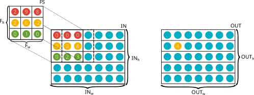
Figure 1. Convolution step with one $3\times 3$ filter ($\mathit{OUT}_{c}=1$), one channel ($\mathit{IN}_{c}=1$) and unitary stride. The solid border square indicates the first window, and the dashed border square represents the second window. The convolution between the filter and the first window results in the yellow element in the output.

A window is the projection of a filter onto the input tensor, resulting in an $\mathit{IN}_{c}\times F_{h}\times F_{w}$ block of elements. Each output element results from the weighted sum of the input elements in a window, with the weights being the corresponding filter elements. The formation of windows from the input tensor and the computation of a convolution output element are illustrated in Figure 1. Each filter slides over $\mathit{IN}$ with stride $s$ in one dimension between computations.

Tiling a convolution consists of dividing the input tensor $\mathit{IN}$, filter set $\mathit{FS}$, and output tensor $\mathit{OUT}$ into tiles that fit in the cache simultaneously. Access to these tiles can be scheduled to take advantage of every cache level in a memory hierarchy.

2.2. Im2Col - Image-to-Column

In the Im2Col + BLAS approach (Chellapilla et al., 2006), an image-to-column transformation expands the input tensor into windows and then multiplies the result by the weight matrix using a highly optimized GEMM routine from a BLAS library. The Im2Col transformation expands the input image by converting each window into a vector of elements and storing this vector as a column of a larger $(\mathit{IN}_{c}\times F_{h}\times F_{w})\times(\mathit{OUT}_{h}\times\mathit{OUT}_{w})$ tensor. The set of filters forms an $\mathit{OUT}_{c}\times(\mathit{IN}_{c}\times F_{h}\times F_{w})$ tensor. A GEMM operation applied to these 2D tensors produces an $\mathit{OUT}_{c}\times(\mathit{OUT}_{h}\times\mathit{OUT}_{w})$ output tensor. This approach performs two data-movement tasks: (a) the Im2Col data rearrangement; and (b) data packing performed by the GEMM routine to increase spatial locality.

2.3. POWER10 and the MMA Engine

SConv uses an ISA extension for convolution operations in the IBM POWER10 architecture. This processor introduces Matrix-Multiply Assist (MMA) (Moreira et al., 2021), a new built-in engine to accelerate tensor operations accessed through an extension of the POWER ISA v3.1. MMA uses POWER10’s 128-bit vector registers (VSRs) as inputs to perform rank-$k$ outer product operations. The result is stored in one of eight new 512-bit accumulator registers representing two-dimensional matrices. The evaluation in this paper indicates that an efficient combination of MMA and VSR operations considerably improves the performance of direct-convolution operations.

3. SConv Compilation Flow

SConv is a solution to convolution that mixes compile-time data transformation for filter packing and efficient code generation to better utilize memory and architecture resources.

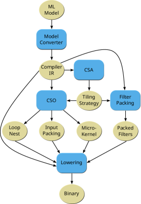
Figure 2. Compilation flow in a machine-learning compiler using SConv to optimize convolutions.

The compilation flow in Figure 2, implemented using ONNX-MLIR and LLVM, can also be used in other compiling frameworks. Blocks are the computation passes and ellipses are the inputs/outputs. After the conversion of a machine-learning model into an Intermediate Representation (IR), the Convolution Slicing Analysis (CSA) algorithm determines — for each convolution layer: (a) the sizes of the data tiles; (b) the tile scheduling, i.e., the order in which they are loaded at execution time; and (c) the number of tiles that are loaded in each step. Together, (b) and (c) determine the tile distribution in the cache hierarchy, which form a Tiling Strategy.

Based on the Tiling Strategy, the Convolution Slicing Optimization (CSO) generates a Loop-Nest macro-kernel for the tiled convolution; an outer-product-based Micro-Kernel to compute a single output tile at peak performance for the architecture; and an Input-tensor Packing routine to rearrange each tile to the required format for the micro-kernel.

For model inference, the filter data is static and filters can be packed at compile-time based on the tiling strategy. The Lowering pass combines the information generated for each convolution with the rest of the compiler IR to produce an executable binary with tiled convolutions. For training, filter data is not static and filters are packed at execution time in the macro-kernel.

The four main components of SConv are CSA (Subsection 4.1), CSO (Subsection 4.2), Input and Filter Packing (Section 6) and the Micro-Kernel (Section 5). The micro-kernel and packing routines are specific to the target architecture. CSA and CSO use architectural information to create a good tiling strategy and to generate code that implement it. The micro-kernel is designed to leverage ISA acceleration extensions and dictates the packing layout and some tiling dimensions.

4. Convolution Slicing

An efficient cache-tiling solution that aims to minimize reuse distance is at the core of a direct-convolution algorithm. SConv accomplishes efficient tiling through two compilation passes: Convolution Slicing Analysis (CSA) is responsible for computing tile sizes, distribution, and scheduling; and Convolution Slicing Optimization (CSO) generates the macro-kernel used to compute the tiled convolution based on the tiling strategy determined by CSA.

4.1. Convolution Slicing Analysis (CSA)

Convolution Slicing Analysis (CSA), a cache-blocking-based algorithm, uses a symbolic simulation heuristic to find a suitable data tiling and scheduling combination that reduces convolution execution time. It aims to maximize input-tensor and filter data reuse on cache memories by: (a) determining the tile size and distribution through the cache hierarchy that maximize cache usage for every level; and (b) selecting the order in which input-tensor/filter tiles are accessed to reduce data movement between the various levels of the cache hierarchy. In this paper $\mathit{IN}^{T},\mathit{FS}^{T}$, and $\mathit{OUT}^{T}$ represent, respectively, the tiles of $\mathit{IN}$, $\mathit{FS}$, and $\mathit{OUT}$.

Each convolution output element is related to an input-tensor window and there is usually an overlap between windows. Thus, each $\mathit{IN}^{T}$ contains multiple windows to leverage micro-kernel vectorization. CSA determines the number of windows available in each $\mathit{IN}^{T}$ and the number of filters in each $\mathit{FS}^{T}$. The tile sizes are given by Equation 1, where, for example, $\lvert\mathit{IN}^{T}\rvert$ represents the size of the input tile $\mathit{IN}^{T}$. Figure 3 shows that $N_{\mathit{win}}$ is the number of windows in $\mathit{IN}^{T}$ and $N_{f}$ is the number of filters used to form $\mathit{FS}^{T}$. The values of $N_{\mathit{win}}$ and $N_{f}$ are a micro-kernel design choice that aims to maximize performance based on the hardware that supports the computation (Section 5).

The CSA algorithm selects tile sizes based on the following constraints:

• the windows in $\mathit{IN}^{T}$ and the filters in $\mathit{FS}^{T}$ are only tiled in their channel dimensions;

• full $F_{h}\times F_{w}$ filters and windows are used in a tile;

• the maximum number of channels ($N_{c}$) is chosen for each tile.

The combination of $N_{\mathit{win}}$ and $N_{f}$ forms $\mathit{OUT}^{T}$, as shown in Equation 1 and Figure 3. $\mathit{DT}$ is the data type size in bytes (e.g., $4$ for float32). Within the constraints above, the CSA algorithm must ensure that a $\mathit{IN}^{T}$, an $\mathit{FS}^{T}$ and an $\mathit{OUT}^{T}$ must fit in L1 cache.

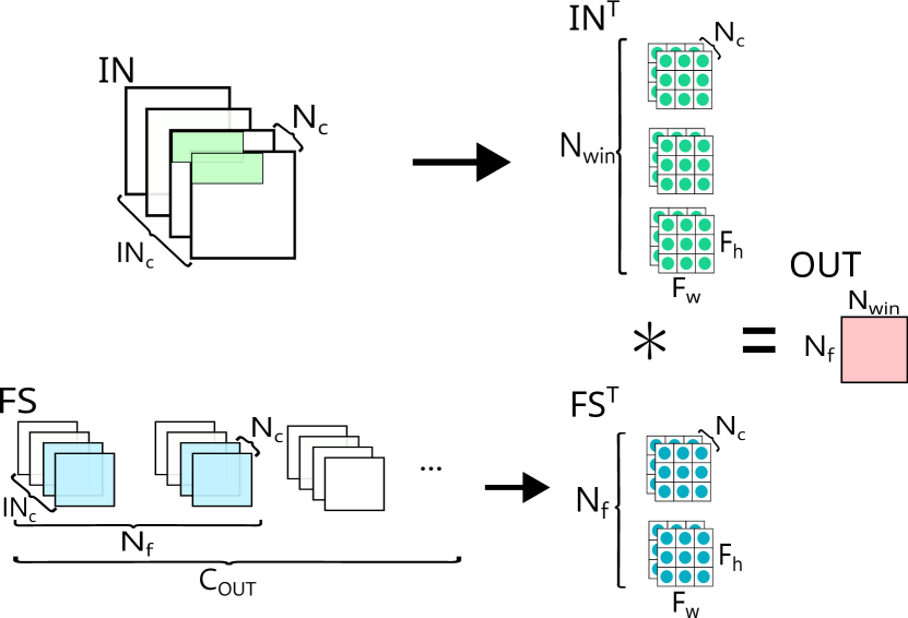
Figure 3. A CSA-tiled convolution, for $F_{h}=F_{w}=3$, before packing.

$$\lvert\mathit{IN}^{T}\rvert = N_{\mathit{win}}\times N_{c}\times F_{h}\times F_{w}\times\mathit{DT}$$

(1) $$\lvert\mathit{FS}^{T}\rvert = N_{f}\times N_{c}\times F_{h}\times F_{w}\times\mathit{DT}$$

$$\lvert\mathit{OUT}^{T}\rvert = N_{\mathit{win}}\times N_{f}\times\mathit{DT}$$

$N_{c}$ specifies the number of input channels in a channel set. When $N_{c}=\mathit{IN}_{c}$ all channels are included in a single $\mathit{IN}^{T}$ and in a single $\mathit{FS}^{T}$, and thus $\mathit{OUT}^{T}$ can be computed in a single step. When $N_{c}<\mathit{IN}_{c}$ each tile combination computes a partial result for an $\mathit{OUT}^{T}$, onto which the results from the rest of the channels need to be accumulated. In this case, the data of $\mathit{OUT}^{T}$ may be evicted from the L1 cache and then loaded again to continue the accumulation. CSA tries to avoid eviction by maximizing $N_{c}$ within the constraints in Equation 2, i.e., the total size of $\mathit{IN}^{T}$, $\mathit{FS}^{T}$, and $\mathit{OUT}^{T}$ has to be less than the available space in the L1 cache — allowing for the space needed for prefetching and intermediate computation, e.g. packing. In Equation 2, the fraction of the L1 cache available for tile storage is represented by $\alpha$, which depends on the hardware and can be tuned to each convolution. An alternative formulation could subtract the estimated space for prefetching and intermediary values from $|\mathit{L1}|$.

(2) $$\begin{split}\lvert\mathit{IN}^{T}\rvert+\lvert\mathit{FS}^{T}\rvert+\lvert\mathit{OUT}^{T}\rvert\leq\lvert\mathit{L1}\rvert\times\alpha\end{split}$$

CSA calculates the number of $\mathit{IN}^{T}$, $\mathit{FS}^{T}$, and $\mathit{OUT}^{T}$ required to compute the convolution. This calculation is done individually for each channel set.

$$\#\mathit{IN}^{T} = \frac{\mathit{OUT}_{h}\times\mathit{OUT}_{w}}{N_{\mathit{win}}}$$

(3) $$\#\mathit{FS}^{T} = \frac{\mathit{OUT}_{c}}{N_{f}}$$

$$\#\mathit{OUT}^{T} = \#\mathit{IN}^{T}\times\#\mathit{FS}^{T}$$

Edge cases arise when the tiling values are not proper divisors of the convolution information. For instance, when $\mathit{IN}_{c}$ is not divisible by $N_{c}$. These cases are handled by computing smaller tiles when necessary, with smaller $N_{c}$, $N_{\mathit{win}}$ and/or $N_{f}$ values.

CSA relies on two possible execution orders when scheduling tiles: (a) Input Stationary (IS), keeps one $\mathit{IN}^{T}$ stationary in L1 cache and reuses it over as many $\mathit{FS}^{T}$ as possible before proceeding to the next $\mathit{IN}^{T}$; (b) Weight Stationary(WS), keeps one $\mathit{FS}^{T}$ stationary in L1, using it to compute multiple $\mathit{OUT}^{T}$ from many $\mathit{IN}^{T}$, before moving to the next $\mathit{FS}^{T}$.

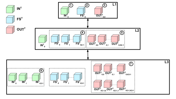
Figure 4. CSA tile distribution over a three-level cache hierarchy with Input Stationary scheduling.

Both the IS and the WS scheduling strategies lead to the specification of $\mathit{K2}$, the number of tiles in the L2 cache, and of $\mathit{K3}$, the number of tiles in the L3 cache. These values are set to use the storage available in each cache level while increasing reuse. The L1 cache must always contain one set of $\mathit{IN}^{T}$, $\mathit{FS}^{T}$, and $\mathit{OUT}^{T}$, which are used for the micro-kernel computation.

Figure 4 illustrates the data movements and computation for the IS schedule. Initially, an $\mathit{IN}^{T}$ is loaded to L1 and kept stationary. Next, a $\mathit{FS}^{T}$ is loaded to L1 so that the micro-kernel is executed to compute an $\mathit{OUT}^{T}$ , which must also fit into L1. While the $\mathit{IN}^{T}$ remains in L1, $(\mathit{K2}-1)$ $\mathit{FS}^{T}$ are in turn brought to L1 to compute other $(\mathit{K2}-1)$ $\mathit{OUT}^{T}$ . The maximum value of $\mathit{K2}$ that satisfies the inequality in Equation 4 ensures that the stationary $\mathit{IN}^{T}$ and the $\mathit{K2}$ $\mathit{FS}^{T}$ and $\mathit{OUT}^{T}$ fit into the L2 cache. The $\mathit{K2}$ $\mathit{FS}^{T}$ kept in L2 are reused by $(\mathit{K3}-1)$ other $\mathit{IN}^{T}$ that are kept in L3 . The maximum value of $\mathit{K3}$ that satisfies the restriction in Equation 5 ensures that a set of $\mathit{K3}$ $\mathit{IN}^{T}$, $\mathit{K2}$ $\mathit{FS}^{T}$ and the results they generate fit into the L3 cache.

The number of times that each tile is loaded to L1 is given as follows:

• If $\mathit{K2}=\#\mathit{FS}^{T}$, then loading each $\mathit{IN}^{T}$ to L1 one time is enough. Otherwise, other $\mathit{K2}$ $\mathit{FS}^{T}$ are loaded from memory to L2, and $\mathit{K3}$ $\mathit{IN}^{T}$ from L3 are loaded to L1 again;

• If $\mathit{K3}\neq\#\mathit{IN}^{T}$, then the same $\mathit{K2}$ $\mathit{FS}^{T}$ are loaded back to L2. In this case, other $\mathit{K3}$ $\mathit{IN}^{T}$ are loaded to L3 and these steps repeat;

• The $\mathit{OUT}^{T}$ are loaded back to L1 for accumulation $((\mathit{IN}_{c}/N_{c})-1)$ times.

In WS scheduling, the order of $\mathit{IN}^{T}$ and $\mathit{FS}^{T}$ are reversed. The share of the caches available to be used in the equations that define $\mathit{K2}$ and $\mathit{K3}$ are represented in Equations 4 – 5 by $\beta$ and $\gamma$. Alternatively, the estimated space needed for packing, prefetching, and other operations, can be subtracted from the cache size.

(4) $$\lvert\mathit{IN}^{T}\rvert+\mathit{K2}\times(\lvert\mathit{FS}^{T}\rvert+\lvert\mathit{OUT}^{T}\rvert)\leq\lvert\mathit{L2}\rvert\times\beta$$

(5) $$\mathit{K3}\times\lvert\mathit{IN}^{T}\rvert+\mathit{K2}\times\lvert\mathit{FS}^{T}\rvert+\mathit{K2}\times\mathit{K3}\times\lvert\mathit{OUT}^{T}\rvert\leq\lvert\mathit{L3}\rvert\times\gamma$$

Exploring the tiling space to find the optimal strategy might lead to very long compilation times. Contrary to other approaches, such as TVM (Chen et al., 2018) or Ansor (Zheng et al., 2020), that consider long compilation and code generation times acceptable (hours), we believe that ML model development cycle should be fast enough (dozens of minutes) to enable the designer to explore many different model architectures. Hence, CSA uses a simple tiling-space exploration heuristic, applied to $N_{c}$, $\mathit{K2}$, and $\mathit{K3}$, that has been shown to produce quality code at reasonable compilation times. Each parameter starts with its highest possible value (e.g. $\mathit{IN}_{c}$ for $N_{c}$), and is halved at each following iteration until all constraints are satisfied. Exploring other tiling-space exploration strategies is left for future work.

CSA decides between IS and WS based on a cost model (Section 4.1.1) using the number of L2, L3, and main memory accesses and estimating the number of cycles for those accesses in each strategy.

4.1.1. Cost Model

$C_{\mathit{TOTAL}}$ is the cost of loading tiles from L2 cache, L3 cache, and main memory. It is the sum of the product of the number of loads from each level and the corresponding cost (in cycles) of each load/store operation at that level (Equation 6). The cost of an L1 hit is not included because every load operation goes through the L1 cache. The cost of reloading an output tile when $N_{c}\neq\mathit{IN}_{c}$ is also not included in the model because it is the same for both the IS and the WS strategies.

(6) $$C_{\mathit{TOTAL}}=C_{\mathit{DRAM}}\times N_{\mathit{DRAM}}+C_{\mathit{L3}}\times N_{\mathit{L3}}+C_{\mathit{L2}}\times N_{\mathit{L2}}$$

(7) $$N_{\mathit{DRAM}}=N_{\mathit{DRAM}_{1}}+N_{\mathit{DRAM}_{2}}$$

The number of DRAM accesses (Equation 7) is the sum of $N_{\mathit{DRAM}_{1}}$, the number of cold misses required to touch every single tile at some point of the convolution execution; and $N_{\mathit{DRAM}_{2}}$, additional touches needed to reload tiles if they are not available in the cache when required.

Let $\mathit{CL}$ be the cache line size of the current architecture. The number of cold misses is given by:

(8) $$N_{\mathit{DRAM}_{1}}=\frac{\mathit{IN}_{c}}{N_{c}}\times\left(\frac{\#\mathit{IN}^{T}\times\lvert\mathit{IN}^{T}\rvert+\#\mathit{FS}^{T}\times\lvert\mathit{FS}^{T}\rvert}{\mathit{CL}}\right)$$

All other equations in this section depend on the analyzed scheduling strategy. The rest of this section will consider the Input Stationary case. For the Weight Stationary cost equations, replace $\#\mathit{IN}^{T}$ and $\lvert\mathit{IN}^{T}\rvert$ with $\#\mathit{FS}^{T}$ and $\lvert\mathit{FS}^{T}\rvert$ and vice-versa.

When all the $\mathit{FS}^{T}$ do not fit simultaneously in the L2 cache, the reloading of tiles during the computation for each set of $\mathit{K3}$ $\mathit{IN}^{T}$ leads to additional DRAM accesses. This data is not available in the L3 cache because it is evicted when loading the other $\mathit{IN}^{T}$ and $\mathit{FS}^{T}$ sets, that use all the available space. Equations 9 – 11 computes $N_{\mathit{DRAM}_{2}}$, the number of additional accesses required.

(9) $$\mathit{FS}^{T}_{\mathit{fitmin}}=\min\left(\left(\frac{\#\mathit{FS}^{T}}{\mathit{K2}}-1\right),1\right)$$

(10) $$\mathit{IN}^{T}_{\mathit{fit}}=\frac{\#\mathit{IN}^{T}}{\mathit{K3}}-1$$

(11) $$N_{\mathit{DRAM}_{2}}=\frac{\mathit{IN}_{c}}{N_{c}}\times\frac{\mathit{FS}^{T}_{\mathit{fitmin}}\times\mathit{IN}^{T}_{\mathit{fit}}\times\#\mathit{FS}^{T}\times\lvert\mathit{FS}^{T}\rvert}{\mathit{CL}}$$

$\mathit{FS}^{T}_{\mathit{fitmin}}$ represents the condition for additional DRAM accesses, i.e. if $\#\mathit{FS}^{T}$ fits in the L2 cache. If the equation evaluates to zero, no reloads are needed. Otherwise, the number of loads from memory is controlled by $\mathit{IN}^{T}_{\mathit{fit}}$, the number of additional $\mathit{IN}^{T}$ sets.

An $\mathit{IN}^{T}$ may need to be loaded from the L3 cache more than once. If there is more than one set of $\mathit{K2}$ $\mathit{FS}^{T}$, the next set will need to be computed with all $\mathit{K3}$ $\mathit{IN}^{T}$ in the L3 cache, so they have to be loaded to L1 again. In the calculation of the number of loads into L3 (Equations 12 – 13), $\mathit{FS}^{T}_{\mathit{fit}}$ controls the number of reloads from the L3 cache with the number of additional $\mathit{FS}^{T}$ sets.

(12) $$\mathit{FS}^{T}_{\mathit{fit}} = \frac{\#\mathit{FS}^{T}}{\mathit{K2}}-1$$

(13) $$N_{\mathit{L3}} = \frac{\mathit{IN}_{c}}{N_{c}}\times\frac{\mathit{FS}^{T}_{\mathit{fit}}\times\#\mathit{IN}^{T}\times\lvert\mathit{IN}^{T}\rvert}{\mathit{CL}}$$

For every $\mathit{IN}^{T}$, all $\mathit{K2}$ $\mathit{FS}^{T}$ need to be loaded from the L2 cache for computation. Since the tiles initially come from memory directly to the L1 cache, one access should be discharged. $N_{\mathit{L2}}$ is calculated using Equation 14.

(14) $$N_{\mathit{L2}}=\frac{\mathit{IN}_{c}}{N_{c}}\times\frac{\left(\#\mathit{IN}^{T}-1\right)\times\#\mathit{FS}^{T}\times\lvert\mathit{FS}^{T}\rvert}{\mathit{CL}}$$

The cost model represents all data movement between cache levels and main memory, and they depend on the scheduling strategy. A lower cost means better tile reuse and cache usage. Thus, the cost should be calculated for both approaches, and the lowest value should be chosen, for each convolution, for that specific architecture.

4.2. Convolution Slicing Optimization (CSO)

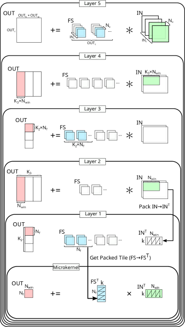
Figure 5. Convolution macro-kernel generated by CSO using CSA’s tiling parameters. Illustrates the process for Input Stationary scheduling.

The Convolution Slicing Optimization (CSO) slices the input, filters, and output based on the tiling sizes and scheduling computed by CSA and generates a macro-kernel to compute the tiled convolution. The main idea is to maximize tile reuse to take advantage of the cache hierarchy.

The input-tensor packing routine (Subsection 6.1) expands the input into windows for one tile and packs the tile such that the elements are in the order required by the micro-kernel. The CSO macro-kernel calls the input-tensor packing routine and iterates over all tiles in the order established by CSA. The loop nest is represented as layers for Input Stationary scheduling in Figure 5. This section details that figure.

For efficiency, the micro-kernel in the innermost loop (Section 5) computes with tiles already loaded into the L1 or L2 caches. Thus, the algorithm implements Packing on Demand: layer two of the loop nest packs input-tensor tiles right before they are used. The filter-packing routine, used in layer 1, returns the already packed tile since the filters have already been packed during the model’s compilation.

The outermost loop (layer five) iterates over channel sets with no reuse between them. Once a channel set is selected, the tiles within this channel set need to be further divided so that a few stay at each cache level. This is done via the $\mathit{K2}$ and $\mathit{K3}$ parameters.

Layers 4 and 2 are responsible for managing all $\mathit{IN}^{T}$. Layer 4 iterates over different sets of $\mathit{K3}$ input-tensor tiles, and layer 2 iterates over a single set, packing one tile at a time. Similarly, Layers 3 and 1 iterate over all $\mathit{FS}^{T}$. Layer 1 calls the micro-kernel, so this setup ensures that every combination of $\mathit{IN}^{T}$ and $\mathit{FS}^{T}$ is computed.

The $\mathit{IN}^{T}$ selected by layer 2 is kept stationary in the L1 cache since it is used with $\mathit{K2}$ $\mathit{FS}^{T}$ in layer 1. When the next $\mathit{IN}^{T}$ is selected, these filter-set tiles are in the L2 cache to be reused. Likewise, $\mathit{IN}^{T}$ are kept in the L3 cache afterward for reuse with the next set of $\mathit{FS}^{T}$.

In Weight Stationary scheduling, the process is the same, switching $\mathit{IN}^{T}$ and $\mathit{FS}^{T}$. Since the $\mathit{IN}^{T}$ need to be packed for the L2 cache in this case, the packing process happens in layer 3 for all $\mathit{K2}$ tiles at once, and each tile is fetched when needed.

5. An Outer-Product Micro-Kernel

The micro-kernel, located in the most internal layer of Figure 5, computes the arithmetic operations that form the convolution. For most efficiency, the micro-kernel should be treated as an extension of the hardware instead of a high-level routine. A micro-kernel implementation is tailored to the architecture and uses any available specific instructions to increase throughput. This work focuses on a single-precision (32-bit) floating-point micro-kernel.

SConv uses an outer-product-based micro-kernel. The outer product is generally useful due to its versatility for computing higher-rank operations and high throughput, computing $n^{2}$ output elements from $2n$ input elements. For those reasons, it is widely used in high-performance linear algebra libraries, and it is being incorporated in CPU ISA extensions such as IBM POWER10 MMA (Moreira et al., 2021). The micro-kernel computes a sum of outer products between vectors of floating-point elements, loaded from memory with unitary stride. A highly optimized implementation of such micro-kernel is found in BLAS GEMM, which can be used as the inner layer of the algorithm, repurposed by the packing layout and macro-kernel. This brings an additional benefit: those architectures with a BLAS implementation can easily integrate their micro-kernel into SConv. Moreover, a new micro-kernel designed for some future architecture could seamlessly be used by both a BLAS library and SConv.

5.1. Micro-Kernel for IBM’s MMA

For the POWER10 architecture, the MMA engine can compute multiple output elements at once. Each input element is used multiple times to compute different output elements. Thus, the input should be split into windows when packing.

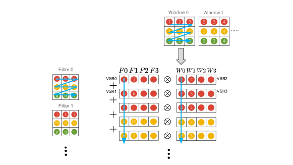
(a)

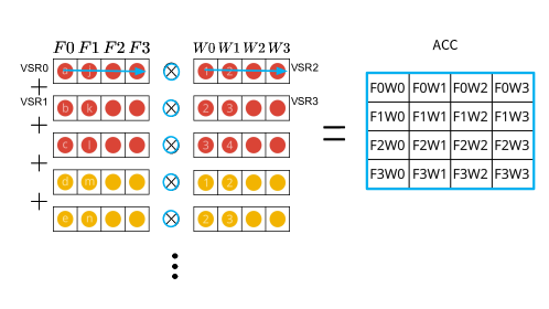
(b)

Figure 6. Execution of a POWER10 convolution micro-kernel for 32-bit floating point. Four filters and four windows are used in each VSR of the outer product.

The outer-product-based design of MMA enables vectorization of the convolution, as shown in Figure 6a. For 32-bit data types, each VSR contains four elements. One VSR contains elements from four different filters and the other from four different windows. An outer product between two VSRs computes sixteen partial output elements, as shown in Figure 6b. In the two-dimensional matrix produced, each row represents a convolution with one filter, and each column represents convolutions with one window. The partial products are accumulated in-place in this accumulator. The accumulated values are stored to memory after the complete set of $F_{h}\cdot F_{w}\cdot N_{c}$ outer product operations have been executed. The resulting data layout is correct for the convolution output, and thus there is no need for unpacking or reordering.

Combining all available VSRs, a larger accumulator can be emulated with a layout-dependent size. Its bigger dimension should be used for computing more windows in each micro-kernel call because there are usually more windows than filters in a convolution. This ”super accumulator” has $8\times 16$ elements in total (Carvalho et al., 2022) and the micro-kernel consumes eight filters and sixteen windows per call.

For POWER10 CSA uses $N_{f}=8$ and $N_{\mathit{win}}=16$ as described in Subsection 4.1.

5.2. Micro-Kernel for Intel’s AVX-512

Even though the Intel Skylake x86 architecture does not feature a matrix engine, the data layout for the input and output structures is the same as for the POWER10 micro-kernel. In this architecture, vector instructions in AVX-512 vector registers emulate the outer-product computation using the following algorithm:

• load two AVX-512 registers with 4 elements (128 bits) each;

• broadcast the elements to fill the rest of each register with copies;

• permute the results so that copies of the same element are consecutive;

• perform a Fused Multiply-Add (FMA) operation between the registers.

This micro-kernel computes $16$ windows ($N_{\mathit{win}}$) and $24$ filters ($N_{f}$) per call. A similar process can be done to emulate outer products in other architectures with SIMD computing.

6. Packing on Demand for the Micro-Kernel

Since the micro-kernel is responsible for computing the convolution and is the innermost step in the loop nest, it should be the focus for maximizing performance. This entails minimizing CPU stalls and data-manipulation overhead. Therefore, the required data should be stored sequentially in memory, in the correct order, and ideally available in cache. Therefore, SConv includes packing steps for both the input tensor and filters, as indicated in layers 2 and 1 from Figure 5, respectively.

The objective of the packing steps is to reshape and, in the input-tensor case, to expand a tile of data into the format required by the micro-kernel. Thus, this format can differ between architectures. The packing routines are called for a single tile at a time and the data is loaded into the L1 cache for the micro-kernel to use thereafter (Packing on Demand).

6.1. Input-Tensor Packing

The input must be expanded into windows, which are then reshaped so that the micro-kernel can be used to compute the convolution. Instead of doing this process in two separate steps as done by Im2Col+BLAS, the SConv input-tensor packing routine combines both into a single pass.

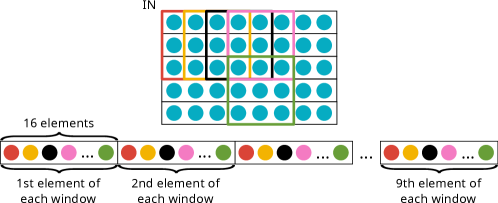
Figure 7. SConv’s input-tensor packing layout for a 16-window micro-kernel, applied on a convolution with $F_{h}=F_{w}=3$, $\mathit{IN}_{c}=1$ and unitary stride. For each of the 16 windows, the elements from the same position are stored sequentially.

Figure 6a illustrates the micro-kernel’s access pattern in the POWER10 architecture. A window’s elements are distributed between multiple outer products, so a vector register contains elements from the same position in different windows. In Figure 6, VSR2 contains the first element of each window, VSR3 has the second element of each window, and so on. Therefore, the elements in memory should follow this pattern. Other outer-product-based micro-kernels, such as the one for Intel Skylake x86, follow this same access pattern.

Figure 7 shows the packing layout derived from the micro-kernel’s access pattern. Elements are loaded multiple times. Thus, the data is packed so that the elements from the same position in every window are stored sequentially in memory. This pattern is repeated for all $N_{c}$ channels in the tile so that the packing routine takes advantage of both spatial and temporal data locality per row, especially in unitary stride convolutions.

6.2. Vector-Based Input Packing

Packing the input tensor in SConv requires data replication because one element can be a part of many windows. In fact, most elements in an input tensor participate in many windows.

The most straightforward way to optimize for multiple loads of the same element is to load from the L1 cache whenever possible. However, when the convolution has a unitary stride, the first element from the next window is the second element from the current window, excluding border cases (as evidenced by Figure 7). Therefore, a shift-left operation with a serial-in element is enough to get the next element from each of the windows in a packed tile.

This observation enables the use of Vector-Based Packing (VBP), where a vector shift operation reduces loads: the next element of each window in a row is obtained by shifting the current set of elements to the left, which can be done by loading all elements into vector registers. This operation is available in most architectures, so the technique is general. Both POWER10 and Intel Skylake x86 provide instructions to shift a pair of vector registers together to the left with the second vector register appended to the right of the first. The least significant element of the first vector register is fed by the most significant element of the second vector register.

Padding the input tensor at the start of the convolution process addresses edge cases. Convolutions with $1\times 1$ filters can also benefit from vector register use, even if no shifts are needed.

6.3. Filter Packing

Filters are loaded in the same way as windows in the micro-kernel. Thus, the packing strategy is similar: a position from each tile filter is packed before advancing to the next, and this process repeats for every channel. However, in contrast with the input tensor, there is no data replication while packing the filters, only the rearrangement of their elements.

Filter packing differs between the two tested architectures because their micro-kernels compute a different number of filters per call.

7. Comparing SConv With Im2Col + BLAS

This experimental evaluation indicates that the strengths of SConv come from the use of faster micro-kernels that are tailored for each architecture, and from the careful packing that reduce cache misses.

7.1. Full-Model Performance Evaluation Using ONNX-MLIR

The SConv prototype evaluated in the two CPU architectures specified in Table 1 is integrated into the ONNX-MLIR framework (Le et al., 2020) to allow for full-model performance evaluation under realistic conditions. The loop nest, input-tensor packing routine and micro-kernel are implemented as a library instead of being completely generated by CSO at compile-time. All the $393$ convolutions found in seven machine-learning models from the ONNX Model Zoo (ONNX, 2019), are executed with SConv. Each model takes one input image, thus the batch is 1.

Name	IBM Power E1050	Intel Xeon Silver 4208
CPU Architecture	IBM POWER10	Intel Cascade Lake (x86)
Matrix/SIMD Engines	MMA/VSX	None/AVX-512
L1 Cache Size	32 kB	32 kB
L2 Cache Size	1 MB	1 MB
L3 Cache Size	4 MB	4 MB
CPU Frequency	4 GHz	2.1 GHz
Matrix/SIMD Units	2/4	0/1
Max Throughput	256 GFLOPS/s	67.2 GFLOPS/s

Table 1. Details of CPU architectures on which tests were conducted.

The baseline, called Base, is an industry-standard convolution algorithm where the input is packed into a patch-matrix using the Im2Col routine from the Caffe framework (Jia et al., 2014), followed by a call to an optimized GEMM routine from the OpenBLAS library (Xianyi et al., [n. d.]). For a fair comparison, the micro-kernels used in SConv are from this library.

Equation 2 and Equations 4 – 5 introduce the $\alpha$, $\beta$, and $\gamma$ parameters to account for extra space needed for non-tile data in each level of the memory hierarchy. These parameters can be tuned for each use case. For this performance evaluation, the values of all three parameters were set to $0.9$ for all convolutions and both machines. Exploration with slight variations around these values revealed that there was no significant performance effects.

Both SConv and Base  use single-precision floating-point datatype, are executed in single-threaded mode, and are compiled with Clang 14 for the x86 architecture and IBM XL C/C++ for Linux 17.1.1 for POWER10. Cache performance measurements for x86 use the Perf Events API from the Linux kernel. All results are averaged over 100 runs, with less than 5% observed standard deviation for both architectures.

7.2. WS $\times$ IS Scheduling

The convolution scheduling, determined by the cost model (Subsection 4.1.1), is sensitive to the micro-kernel shape ($N_{f}\times N_{\mathit{win}}$). The POWER10 micro-kernel computes $8\times 16$ elements, while the x86 micro-kernel computes $24\times 16$ elements. The change in the $N_{f}$ value leads to a larger $\mathit{FS}^{T}$, which may favor its reuse in the L1 cache. This difference leads to the selection of weight-stationary scheduling for x86, and input-stationary scheduling for POWER10.

7.3. SConv Outperforms Base in Every Model

Table 2 shows the convolution-only speedup and the whole-model speedup including every convolution from each model. SConv outperforms Base in every model on both architectures with convolution speedups ranging from 12% to 46%. As expected, higher speedups are observed in models with large convolutions, such as VGG-16 and ResNet-18. The fraction of the time spent in convolution in ONNX-MLIR determines the effect of using SConv over Base in the whole-model performance. On average, whole models are between 15% and 18% faster.

Model	Convolution Speedup		Model Speedup		Convolution Time Share
	x86	P10	x86	P10	x86	P10
GoogleNet (Szegedy et al., 2015)	1.18	1.26	1.10	1.10	0.49	0.43
InceptionV2 (Ioffe and Szegedy, 2015)	1.21	1.28	1.16	1.17	0.76	0.62
ResNet-18 (He et al., 2016)	1.26	1.46	1.25	1.42	0.93	0.82
ResNet-50 (He et al., 2016)	1.13	1.28	1.09	1.17	0.87	0.72
ResNet-152 (He et al., 2016)	1.16	1.28	1.13	1.21	0.91	0.77
SqueezeNet (Iandola et al., 2016)	1.12	1.27	1.16	1.13	0.74	0.55
VGG-16 (Simonyan and Zisserman, 2015)	1.27	1.28	1.16	1.12	0.70	0.39
Geo Mean	1.19	1.30	1.15	1.18	0.76	0.59

Table 2. SConv performance speedup over Base in machine-learning models.

A more in-depth performance analysis needs to examine the performance changes in individual convolutions. Figure 8 shows the results for all individual convolutions sorted by speedup. For about 90% of the convolutions, SConv outperforms Base. The maximum speedup for x86 is 2.1$\times$, and for POWER10 is 1.9$\times$. SConv reaches 77% of the theoretical peak throughput in POWER10 and 90% in x86. Subsection 7.5 explores what is causing SConv to underperform Base in about 10% of the convolutions.

(a) x86

(b) POWER10

Figure 8. SConv performance speedup against Base for each of the 393 individual convolutions from the evaluated machine learning models. The x-axis is sorted by speedup (y-axis). Base’s performance is normalized to 1. The graphs also indicate the percentage of convolutions in which SConv outperforms Base.

(a) x86

(b) POWER10

Figure 9. SConv performance speedup against BLAS for each of the 219 pointwise convolutions from the evaluated machine learning models. The x-axis is sorted by speedup (y-axis). BLAS’ performance is normalized to 1. The graphs also indicate the percentage of pointwise convolutions in which SConv outperforms BLAS.

7.4. Faster Micro-Kernels Make Packing Time More Relevant

(a) x86

(b) POWER10

Figure 10. Breakdown of each model’s total convolution time distributed between packing, micro-kernel (mK) and other steps (Others), for Base and SConv.

Figure 10 shows the convolution execution time divided into (a) ”Packing”, including Im2Col and GEMM packing; (b) ”mK”, the micro-kernel execution, which is the same for both approaches; (c) ”Others”, which represents the remaining boilerplate code (e.g., bias, control code, padding, etc.) that is different for Base and SConv. In SConv, packing has a smaller contribution to the execution time in comparison with Base. SConv provides three major improvements in packing: elimination of the Im2Col step, reduction of unnecessary loads by Vector-Based Packing, and optimization of filter-packing at compile-time.

The x86 results show that Base has, on average, 26% of its execution time dedicated to packing (20% — 32%), while SConv’s packing share averages 10% (6% — 15%). The POWER10 results indicate a larger improvement, with Base’s packing share averaging 39% (36% — 47%) and SConv’s averaging 10% (7% — 13%), which is a packing time improvement of 3.0x on x86 and 5.0x on POWER10. The improvement range is 2.0x — 3.9x on x86 and 3.6x — 7.2x on POWER10. Faster hardware-supported micro-kernel makes the packing time more significant in the overall execution. This effect is evident in the better POWER10 results, which translates to overall speedup in Table 2 and Figure 8.

Packing data is most significant for large convolutions, such as those in ResNet18 and VGG16, that contribute most to the model time. Large convolutions are the most sensitive to some of the improvements in SConv, such as VBP and the elimination of Im2Col. Thus, packing optimizations are the main contributors to the results shown in Subsection 7.3.

7.5. Im2Col is Not Needed for Pointwise Convolutions

A pointwise convolution comprises $1\times 1$ windows with unitary stride. Such convolutions are frequently found in ML models — $219$ out of the $393$ (55%) convolutions in our experimental evaluation. Even though they are usually smaller and faster to compute, they often do not contribute as much to the model execution time. For a pointwise convolution, the Im2Col transformation produces a simple copy of the input matrix, and thus Im2Col can be skipped altogether. A pointwise convolution can be trivially reduced to a GEMM operation, thus SConv is compared directly with the BLAS library’s GEMM routine. Therefore, SConv does not have the advantage of fewer packing steps or Vector-Based Packing in these convolutions.

SConv’s results for these convolutions, shown in Figure 9, have a pattern that matches, to some degree, the one in Figure 8, indicating good performance even when there is no Im2Col overhead in the baseline. SConv outperforms BLAS GEMM in 87% of all pointwise convolutions on x86, and 83% on POWER10, with larger average improvements in the positive cases than slowdowns in the negative ones. These results evidence the efficiency of CSA’s tiling strategy for different convolution shapes and the advantage of packing filters at compile-time. Compile-time packing is only important in convolutions with many filters and channels and small $\mathit{IN}_{h}$ and $\mathit{IN}_{w}$, and this is reflected in which convolutions achieve higher speedups.

Most convolutions for which Base outperforms SConv are pointwise: 93% on POWER10 and 78% on x86. For instance, the largest pointwise convolutions found in the tested models have $\mathit{IN}_{h}=\mathit{IN}_{w}=56$, and are consistently faster in Base. These cases fit the best-performance scenario of the BLAS GEMM routine because the inner dimension ($\mathit{IN}_{c}$) is small compared to the dimensions of the output matrix (Zhang et al., 2018). Furthermore, filter packing has a smaller impact on the overall execution time when the input tensor is large.

7.6. SConv Reduces Cache Misses in All Levels of Cache

(a) L1

(b) L2

(c) L3

Figure 11. Breakdown of each model’s cache miss performance in each level, for Base and SConv on x86. Shows the percentage of cache misses in each level from the total loads.

The main goal of the slicing strategy in SConv is to improve cache performance. The Im2Col step is bad for cache performance since most tiles, after expansion, need to be reloaded from a more distant cache level or DRAM for GEMM packing and computation. Removing Im2Col allows for Packing On Demand, which improves cache locality by keeping the tiles in the cache after packing for the micro-kernel. Furthermore, the tiling strategy determined by CSA optimizes tile reuse by scheduling in order to minimize the data flow between memory levels. However, the addition of explicit padding in SConv adds extra loads which may lead to more cache misses.

SConv has fewer loads than Base in 65% of all tested convolutions (246). Even when SConv has more loads than Base (147, 35%), the impact on cache misses is not significant: SConv has more L1 misses on 0.5% of the convolutions (2), more L2 misses on 5% (20) and more L3 misses on 4% (15). In these cases, the difference is small.

The miss rates shown in Figure 11 are for all loads in the model. For SConv, around 90% of all loads resolve in L1 cache, compared with 83% for Base — a 1.9$\times$ improvement. The difference between the methods increases at lower cache levels. On average, SConv has 5.9x fewer L2 misses and 9.9x fewer L3 misses, though both represent a small percentage of the total number of loads. In the case of VGG-16, SConv’s improvements on larger convolutions resulted in a big drop in L3 misses because, with the input not fitting in cache, data has to be reloaded from DRAM in Base, which does not happen in SConv. Not only SConv is better at minimizing expensive memory operations, it also often requires fewer load operations to compute the convolution.

8. Related Work

Chellapilla et al. proposed the computation of convolution using the Im2Col transformation to reduce the problem to GEMM and solve it using a BLAS library (Chellapilla et al., 2006). This approach is used in many machine learning frameworks, such as TensorFlow (Abadi et al., 2016), PyTorch (Paszke et al., 2019) and Caffe (Jia et al., 2014). The BLAS’s GEMM routine already contains packing steps, thus two separate steps require data manipulation: expansion (Im2Col) and packing. This approach has a large memory footprint because of the large matrix resulting from Im2Col. Also, the GEMM tiling can be inefficient when the inner dimension is large. Other authors address the memory footprint issue while still using BLAS GEMM as a foundation to solve the convolution problem (Vasudevan et al., 2017; Cho and Brand, 2017; Anderson et al., 2020). However, they still use GEMM’s tiling with multiple data-manipulation steps.

Zhang et al. (Zhang et al., 2018) discuss the limitations and inefficiencies of the Im2Col + BLAS convolution algorithm and present an argument for using direct convolution instead. They use a model architecture with fused multiply-add instructions to explore cache blocking, and data reuse, given a friendly memory layout. Unlike the work proposed by Zhang et al. , SConv explores more scheduling strategies and tile distribution in the cache hierarchy, provides a template that can be used in different architectures and does not impose a different memory layout. Thus SConv can be deployed in other AI/ML frameworks without changing any other operator implementation.

Goto and de Gejin (Goto and Geijn, 2008) introduce the idea of exploiting an optimized micro-kernel (called ”inner-kernel”) by tiling the problem in an external macro-kernel. These tiles are then packed to a friendly layout for the micro-kernel. The CSA algorithm resembles the algorithm proposed by Goto and de Gejin in its functionalities, but it applies the strategy to convolution instead of applying it to GEMM.

Juan et al. (Juan et al., 2020) modify the BLIS library’s (Van Zee and van de Geijn, 2015) GEMM routine to apply Im2Col in its packing step. The result is a convolution and GEMM hybrid named ConvGEMM, which takes advantage of Goto and de Gejin’s GEMM tiling and structure with the Im2Col transformation applied on the fly, eliminating the double-packing problem. This process is similar to Packing on Demand, but the tiling is still GEMM-based, that is, 2D slicing without the concept of scheduling, and therefore has different cache usage, tile reuse, and packing patterns. A similar attempt to adapt GEMM to a convolution algorithm by lazy Im2Col packing was made for GPU hardware by Chetlur et al. (Chetlur et al., 2014). Dukhan proposes an indirect-convolution algorithm that modifies GEMM all the way to the micro-kernel to avoid materializing the Im2Col matrix in memory (Dukhan, 2019).

Korostelev et al. (Korostelev et al., 2022) combine the ideas of modifying the GEMM routine and decomposing convolution into multiple GEMM operations (Anderson et al., 2020) to create a new method that avoids packing redundancy while keeping the overall GEMM structure (tiling, packing, micro-kernel). Contrary to the approach in SConv, (Korostelev et al., 2022) works only on unitary stride convolutions and improves only non-pointwise convolutions. Moreover, their experiments focus on isolated convolutions and do not provide results for complete models.

Space exploration tools such as TVM (Chen et al., 2018) and Ansor (Zheng et al., 2020) can change loop order and tile size using machine-learning techniques and a cost model. Due to the highly automated nature of these tools, total hardware usage is harder to achieve in more complex architectures. The ample tiling space also leads to long compilation and code-generation times, hindering the ML model design-time efficiency.

This project follows the work done by Sousa et al. (Sousa et al., 2021) in tiling 3D convolutions targeting NPUs, by generalizing its tiling analysis for CPUs in the CSA pass. In that work, the Input Stationary and Weight Stationary scheduling strategies are used in a different context, and the modeling focuses on taking advantage of memory bursts while loading data to the scratchpad memories.

Following the work from Zhang et al. (Zhang et al., 2018), Barrachina et al. (Barrachina et al., 2023) propose two new direct-convolution algorithms for the NHWC layout (batch $N$, height $H$, width $W$, and channels $C$) on ARM processors. Like SConv, they tile in the channel dimension and use a BLAS micro-kernel. In SConv, however, besides considering the partitioning of the input tensor and of the filter set, tiling also considers the two scheduling alternatives — input or weight stationary — and the tile distribution over the cache hierarchy. SConv shows that direct convolution can benefit from: (a) novel ISA extensions, such as the POWER10 MMA, for faster tensor-algebra computation; (b) vector-register extensions, such as Intel x86 AVX and POWER VSX, to implement Vector-Based Packing. The experimental evaluation demonstrates the flexibility of SConv by using two different CPU architectures and the common NCHW layout.

9. Conclusion and Future Work

As stated in the introduction, the objective of the algorithm presented in this paper is to provide a good implementation of direct convolution for different CPU architectures. SConv achieves this goal, outperforming Im2Col + BLAS in experiments performed in realistic conditions with full machine learning model inference (Subsection 7.3) on both tested architectures by reducing total data manipulation time (Subsection 7.4). SConv also outperforms regular BLAS GEMM when computing pointwise convolutions in over 83% of the 219 instances tested (Subsection 7.5).

As for future work, some interesting paths can be pursued. Currently, the CSA tiling analysis pass creates tiles based solely on micro-kernel information and the $\mathit{IN}_{c}$ value. More robust space exploration can be done by exploiting other dimensions of $\mathit{IN}^{T}$ and $\mathit{FS}^{T}$. This change may further improve cache locality by better utilizing the L1 cache. CSA’s optimization heuristic may also be improved if a binary search is used to find a better approximation for the tile size. Moreover, since the approach is integrated with machine-learning compilers, a fully code-generation-based implementation can leverage compile-time information to simplify operations such as padding and remove boilerplate code overhead. Finally, a hybrid solution with Im2Col + BLAS might perform best for each convolution.

References

- (1)
- Abadi et al. (2016) Martín Abadi, Paul Barham, Jianmin Chen, Zhifeng Chen, Andy Davis, Jeffrey Dean, Matthieu Devin, Sanjay Ghemawat, Geoffrey Irving, Michael Isard, Manjunath Kudlur, Josh Levenberg, Rajat Monga, Sherry Moore, Derek G. Murray, Benoit Steiner, Paul Tucker, Vijay Vasudevan, Pete Warden, Martin Wicke, Yuan Yu, and Xiaoqiang Zheng. 2016. TensorFlow: A System for Large-Scale Machine Learning. In Proceedings of the 12th USENIX Conference on Operating Systems Design and Implementation (Savannah, GA, USA) (OSDI’16). USENIX Association, USA, 265–283.
- Anderson et al. (2020) Andrew Anderson, Aravind Vasudevan, Cormac Keane, and David Gregg. 2020. High-Performance Low-Memory Lowering: GEMM-based Algorithms for DNN Convolution. In 2020 IEEE 32nd International Symposium on Computer Architecture and High Performance Computing (SBAC-PAD). 99–106. https://doi.org/10.1109/SBAC-PAD49847.2020.00024
- Barrachina et al. (2023) Sergio Barrachina, Adrián Castelló, Manuel F. Dolz, Tze Meng Low, Héctor Martínez, Enrique S. Quintana-Ortí, Upasana Sridhar, and Andrés E. Tomás. 2023. Reformulating the direct convolution for high-performance deep learning inference on ARM processors. Journal of Systems Architecture 135 (2023), 102806. https://doi.org/10.1016/j.sysarc.2022.102806
- Carvalho et al. (2022) João P. L. de Carvalho, José E. Moreira, and José Nelson Amaral. 2022. Compiling for the IBM Matrix Engine for Enterprise Workloads. IEEE Micro (2022), 1–8. https://doi.org/10.1109/MM.2022.3176529
- Chellapilla et al. (2006) Kumar Chellapilla, Sidd Puri, and Patrice Simard. 2006. High Performance Convolutional Neural Networks for Document Processing. In Tenth International Workshop on Frontiers in Handwriting Recognition, Guy Lorette (Ed.). Université de Rennes 1, Suvisoft, La Baule (France). https://hal.inria.fr/inria-00112631
- Chen et al. (2018) Tianqi Chen, Thierry Moreau, Ziheng Jiang, Lianmin Zheng, Eddie Yan, Meghan Cowan, Haichen Shen, Leyuan Wang, Yuwei Hu, Luis Ceze, Carlos Guestrin, and Arvind Krishnamurthy. 2018. TVM: An Automated End-to-End Optimizing Compiler for Deep Learning. In Proceedings of the 13th USENIX Conference on Operating Systems Design and Implementation (Carlsbad, CA, USA) (OSDI’18). USENIX Association, USA, 579–594.
- Chetlur et al. (2014) Sharan Chetlur, Cliff Woolley, Philippe Vandermersch, Jonathan M. Cohen, John Tran, Bryan Catanzaro, and Evan Shelhamer. 2014. cuDNN: Efficient Primitives for Deep Learning. ArXiv abs/1410.0759 (2014).
- Cho and Brand (2017) Minsik Cho and Daniel Brand. 2017. MEC: Memory-Efficient Convolution for Deep Neural Network. In Proceedings of the 34th International Conference on Machine Learning - Volume 70 (Sydney, NSW, Australia) (ICML’17). JMLR.org, 815–824.
- Dukhan (2019) Marat Dukhan. 2019. The Indirect Convolution Algorithm. ArXiv abs/1907.02129 (2019).
- Goto and Geijn (2008) Kazushige Goto and Robert A. van de Geijn. 2008. Anatomy of High-Performance Matrix Multiplication. ACM Trans. Math. Softw. 34, 3, Article 12 (may 2008), 25 pages. https://doi.org/10.1145/1356052.1356053
- Guennebaud et al. (2010) Gaël Guennebaud, Benoît Jacob, et al. 2010. Eigen v3. http://eigen.tuxfamily.org.
- He et al. (2016) Kaiming He, Xiangyu Zhang, Shaoqing Ren, and Jian Sun. 2016. Deep Residual Learning for Image Recognition. In 2016 IEEE Conference on Computer Vision and Pattern Recognition (CVPR). 770–778. https://doi.org/10.1109/CVPR.2016.90
- Iandola et al. (2016) Forrest N. Iandola, Matthew W. Moskewicz, Khalid Ashraf, Song Han, William J. Dally, and Kurt Keutzer. 2016. SqueezeNet: AlexNet-level accuracy with 50x fewer parameters and ¡1MB model size. ArXiv abs/1602.07360 (2016).
- Ioffe and Szegedy (2015) Sergey Ioffe and Christian Szegedy. 2015. Batch Normalization: Accelerating Deep Network Training by Reducing Internal Covariate Shift. In Proceedings of the 32nd International Conference on International Conference on Machine Learning - Volume 37 (Lille, France) (ICML’15). JMLR.org, 448–456.
- Jia et al. (2014) Yangqing Jia, Evan Shelhamer, Jeff Donahue, Sergey Karayev, Jonathan Long, Ross Girshick, Sergio Guadarrama, and Trevor Darrell. 2014. Caffe: Convolutional Architecture for Fast Feature Embedding. arXiv preprint arXiv:1408.5093 (2014).
- Juan et al. (2020) P. San Juan, A. Castello, M. F. Dolz, P. Alonso-Jorda, and E. S. Quintana-Orti. 2020. High Performance and Portable Convolution Operators for Multicore Processors. In 2020 IEEE 32nd International Symposium on Computer Architecture and High Performance Computing (SBAC-PAD). IEEE Computer Society, Los Alamitos, CA, USA, 91–98. https://doi.org/10.1109/SBAC-PAD49847.2020.00023
- Korostelev et al. (2022) Ivan Korostelev, João P. L. de Carvalho, José Moreira, and José Nelson Amaral. 2022. YaConv: Convolution with Low Cache Footprint. ACM Trans. Archit. Code Optim. (dec 2022). https://doi.org/10.1145/3570305 Just Accepted.
- Le et al. (2020) Tung D. Le, Gheorghe-Teodor Bercea, Tong Chen, Alexandre E. Eichenberger, Haruki Imai, Tian Jin, Kiyokuni Kawachiya, Yasushi Negishi, and Kevin O’Brien. 2020. Compiling ONNX Neural Network Models Using MLIR. ArXiv abs/2008.08272 (2020).
- Moreira et al. (2021) José E. Moreira, Kit Barton, Steven Battle, Peter Bergner, Ramon Bertran, Puneeth Bhat, Pedro Caldeira, David Edelsohn, Gordon Fossum, Brad Frey, Nemanja Ivanovic, Chip Kerchner, Vincent Lim, Shakti Kapoor, Tulio Machado Filho, Silvia Melitta Mueller, Brett Olsson, Satish Sadasivam, Baptiste Saleil, Bill Schmidt, Rajalakshmi Srinivasaraghavan, Shricharan Srivatsan, Brian W. Thompto, Andreas Wagner, and Nelson Wu. 2021. A matrix math facility for Power ISA(TM) processors. CoRR abs/2104.03142 (2021). arXiv:2104.03142 https://arxiv.org/abs/2104.03142
- ONNX (2019) ONNX 2019. ONNX Model Zoo. Retrieved June 26th, 2022 from https://github.com/onnx/models
- Paszke et al. (2019) Adam Paszke, Sam Gross, Francisco Massa, Adam Lerer, James Bradbury, Gregory Chanan, Trevor Killeen, Zeming Lin, Natalia Gimelshein, Luca Antiga, Alban Desmaison, Andreas Kopf, Edward Yang, Zachary DeVito, Martin Raison, Alykhan Tejani, Sasank Chilamkurthy, Benoit Steiner, Lu Fang, Junjie Bai, and Soumith Chintala. 2019. PyTorch: An Imperative Style, High-Performance Deep Learning Library. In Advances in Neural Information Processing Systems 32, H. Wallach, H. Larochelle, A. Beygelzimer, F. d'Alché-Buc, E. Fox, and R. Garnett (Eds.). Curran Associates, Inc., 8024–8035. http://papers.neurips.cc/paper/9015-pytorch-an-imperative-style-high-performance-deep-learning-library.pdf
- Simonyan and Zisserman (2015) Karen Simonyan and Andrew Zisserman. 2015. Very Deep Convolutional Networks for Large-Scale Image Recognition. CoRR abs/1409.1556 (2015).
- Sousa et al. (2021) Rafael Sousa, Byungmin Jung, Jaehwa Kwak, Michael Frank, and Guido Araujo. 2021. Efficient Tensor Slicing for Multicore NPUs using Memory Burst Modeling. In 2021 IEEE 33rd International Symposium on Computer Architecture and High Performance Computing (SBAC-PAD). IEEE Computer Society, Los Alamitos, CA, USA, 84–93. https://doi.org/10.1109/SBAC-PAD53543.2021.00020
- Szegedy et al. (2015) C. Szegedy, Wei Liu, Yangqing Jia, P. Sermanet, S. Reed, D. Anguelov, D. Erhan, V. Vanhoucke, and A. Rabinovich. 2015. Going deeper with convolutions. In 2015 IEEE Conference on Computer Vision and Pattern Recognition (CVPR). IEEE Computer Society, Los Alamitos, CA, USA, 1–9. https://doi.org/10.1109/CVPR.2015.7298594
- Van Zee and van de Geijn (2015) Field G. Van Zee and Robert A. van de Geijn. 2015. BLIS: A Framework for Rapidly Instantiating BLAS Functionality. ACM Trans. Math. Software 41, 3 (June 2015), 14:1–14:33. https://doi.acm.org/10.1145/2764454
- Vasudevan et al. (2017) Aravind Vasudevan, Andrew Anderson, and David Gregg. 2017. Parallel Multi Channel convolution using General Matrix Multiplication. In 2017 IEEE 28th International Conference on Application-specific Systems, Architectures and Processors (ASAP). 19–24. https://doi.org/10.1109/ASAP.2017.7995254
- Xianyi et al. ([n. d.]) Zhang Xianyi, Martin Kroeker, Werner Saar, Wang Qian, Zaheer Chothia, Chen Shaohu, and Luo Wen. [n. d.]. OpenBLAS: An optimized BLAS library. https://www.openblas.net/
- Zhang et al. (2018) Jiyuan Zhang, Franz Franchetti, and Tze Meng Low. 2018. High Performance Zero-Memory Overhead Direct Convolutions. In Proceedings of the 35th International Conference on Machine Learning (Proceedings of Machine Learning Research, Vol. 80), Jennifer Dy and Andreas Krause (Eds.). PMLR, 5776–5785. http://proceedings.mlr.press/v80/zhang18d.html
- Zheng et al. (2020) Lianmin Zheng, Chengfan Jia, Minmin Sun, Zhao Wu, Cody Hao Yu, Ameer Haj-Ali, Yida Wang, Jun Yang, Danyang Zhuo, Koushik Sen, Joseph E. Gonzalez, and Ion Stoica. 2020. Ansor: Generating High-Performance Tensor Programs for Deep Learning. In Proceedings of the 14th USENIX Conference on Operating Systems Design and Implementation (OSDI’20). USENIX Association, USA, Article 49, 17 pages.