Perturbative dynamic renormalization of scalar field theories in statistical physics
Nikos Papanikolaou and Thomas Speck
Institute for Theoretical Physics IV, University of Stuttgart, 70569 Stuttgart, Germany thomas.speck@itp4.uni-stuttgart.de
Abstract
Renormalization is a powerful technique in statistical physics to extract the large-scale behavior of interacting many-body models. These notes aim to give an introduction to perturbative methods that operate on the level of the stochastic evolution equation for a scalar field (e.g., density), including systems that are driven away from equilibrium and thus lack a free energy. While there is a large number of reviews and lecture notes, many are somewhat scarce on technical details and written in the language of quantum field theory, which can be more confusing than helpful. Here we attempt a minimal and concise yet pedagogical introduction to dynamic renormalization in the language of statistical physics with a strong focus on how to actually perform calculations. We provide a symbolic algebra implementation of the discussed techniques including Jupyter notebooks of two illustrations: the KPZ equation and a neural network model.
1 Introduction
In statistical physics, we often encounter dynamic (or “kinetic”) equations of the type
| (1) |
describing the stochastic evolution of a real-valued scalar field in dimensions (). This could be the density change of a monocomponent fluid, related to the composition of a binary mixture, or the (relative) height of a film covering a surface. In all these cases, we might want to quantify the behavior at large scales. The details of the specific model under scrutiny are encoded in the function of the field and its derivatives, which we assume can be parametrized by a set of model parameters . Since is already a coarse-grained description of the microscopic degrees of freedom it is accompanied by a noise field .
We will not discuss how to derive Eq. (1) from a microscopic model, for which there is no unique answer (for an insightful discussion, see Ref. 1). Importantly, the functional form of is largely determined by symmetry considerations and conservation laws. This entails that rederiving the evolution equation on a coarser length scale, we obtain the same functional form but now with renormalized parameters , which thus become functions of the length scale, . The task of renormalization is to obtain the functional dependence for the model parameters. Mathematically, there is a clear analogy with the energy scale in particle physics, and indeed the confluence of both fields has led to one of the major breakthroughs, Wilson’s renormalization group [2]. Its success is due in no small part to the fact that fixed points of this renormalization “flow” encode the universal behavior of scale-free systems and close to critical points.
As an example, assuming that our model is invariant under the inversion as well as rotational symmetry, an expansion to lowest order yields
| (2) |
where we treat both cases of a non-conserved field (, known as model A) and a conserved field (, model B).111These names stem from the classification of Hohenberg and Halperin [3], see Table I therein. A conserved quantity is one for which the integral does not change with time. It implies that we have the continuity equation with current field . This Ginzburg-Landau model is characterized by the parameters , the exact expressions of which follow from the specific microscopic model.
Here we describe how the renormalization procedure can be performed directly on the level of the evolution equation (1), which has been termed “dynamic renormalization group”. A big advantage is that both equilibrium and (driven) non-equilibrium systems can be treated. Early applications include ferromagnets [4], the stochastic Navier-Stokes and Burgers equation [5], as well as the famous KPZ equation [6]. More recent applications are on the conserved KPZ equation [7], self-organized criticality [8], active nematics [9], and in particular on the collective behavior of self-propelled agents [10, 11, 12, 13, 14, 15, 16].
Actual calculations tend to look somewhat complicated and even intimidating. The purpose of these notes is to expose the minimal “machinery” to obtain one-loop flow equations and to study their properties. By no means are they a replacement for more detailed reviews [3], lecture notes [17], and books [18, 19] on renormalization. For completeness, we point out that stochastic dynamic equations can be transformed into a stochastic action (known as Doi-Peliti [20, 21] and Martin-Siggia-Rose [22, 23] formalisms), for which methods from (quantum) field theory are directly applicable. It does, however, add another layer of complexity and for the sake of simplicity we will not discuss it here.
2 Setting the stage
2.1 Linear theory
Neglecting all non-linear terms, we have . We switch to Fourier space through
| (3) |
where we use the same symbol for the field but with different arguments. The linearized evolution equation (1) then reads
| (4) |
with solution , where we have defined the bare propagator
| (5) |
with for later use. Throughout, we will write for the magnitude of the wave vector (and analogously for other wave vectors). For the noise correlations, we will employ
| (6) |
where, for ease of notation, we have combined frequency and wave vector into the single vector with components. Note that for a conserved field the factor suppresses fluctuations of the integrated field as required. The strength of the noise is quantified by the coefficient . For dynamics obeying detailed balance, the fluctuation-dissipation theorem constraints to be related to the temperature but in the following we will mostly treat it as another free model parameter.
It is now straightforward to calculate the field correlations
| (7) |
with the dynamic structure factor
| (8) |
The static structure factor follows immediately as
| (9) |
independent of . Clearly, we can construct one length scale, , which is the correlation length governing the exponential decay of correlations in real space. With this correlation length, the static structure factor becomes
| (10) |
For the correlation length diverges with .
2.2 Basic idea of renormalization
Our model is useful down to a length scale (typically related to the particle size or the lattice spacing) below which we have no further information. In Fourier space this implies that . Let us collect the model parameters into the vector depending on the microscopic cut-off. Now we integrate out spatial features on length scales smaller than with a factor . We thus lose microscopic information (corresponding to large ) and consequently will need new parameters to describe the evolution of the field.
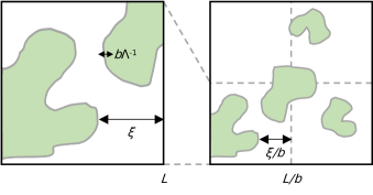
Before we repeat this step to get to an even coarser scale, let us “zoom out” by the factor and look at a larger portion of our system (Fig. 1). Holding the absolute size fixed, this means that coordinates in our original system have shrunk to . Moreover, the size of any “structure” has shrunk by the same factor, in particular the correlation length . Note that this step restores the size of the smallest discernible features to (with respect to ).222As an analogy, consider looking at the system through a microscope at maximal magnification. You then reduce the magnification by a factor looking at a larger portion but with fixed field of view and fixed resolution (say, the size of a pixel). An excellent visualization for the Ising model can be found here: https://www.youtube.com/watch?v=MxRddFrEnPc. Repeating this procedure induces an evolution, a “flow” in model space, during which we zoom out further and further. For an infinitesimal step we find
| (11) |
with flow equations implying the solution of model parameters as a function of . Keeping explicitly track of the scale yields and thus is the actual value of the cut-off with initial value .
The remaining task is to find the functions . Of particular interest are fixed points and the evolution around these fixed points. Their importance can be appreciated by noting that any initial correlation length will flow to except for points in our model space where the correlation length diverges, which will be mapped to critical fixed points.
2.3 Scaling dimensions
Implementing the rescaling step amounts to defining new wave vectors together with , where is the dynamical exponent. Inserting both rescaled quantities into the bare propagator [Eq. (5)] yields
| (12) |
with and . While the functional form of is the same, the model parameters have changed. Clearly, the correlation length indeed transforms as a length (with ). In the vicinity of critical points any quantity changes under rescaling as with called the scaling dimension of . If a scaling dimension is negative then it is called irrelevant: Going to larger scales (large ) the influence of is diminished and eventually vanishes. Correspondingly, is called relevant and the borderline marginal. Demanding that the dynamic equation Eq. (1) is invariant leads to another relation: the left side acquires a factor and, therefore, the noise term scales with [cf. Eq. (6)] and thus . Of particular importance is the Gaussian fixed point (G) at which all non-linear terms become irrelevant and we are left with the linear theory introduced in Sec. 2.1.
To get a different view on scaling we briefly return to real space. The Fourier transform of [Eq. (9)] yields the static correlations
| (13) |
for ignoring numerical factors. If we demand that the functional form of these correlations does not change–we say that they are scale invariant–then a rescaling of lengths on the right-hand side has to be compensated by a rescaling of the field, , with “naive” scaling dimension . In general, the scaling dimension of the field is
| (14) |
with known as the anomalous dimension (not to be confused with the noise field). Moreover, assuming that is constant (as in thermal equilibrium, ), we find [3].
3 Graphical corrections
3.1 Perturbation series and vertex functions
We now include non-linear terms into the evolution equation (4). The -th power of the field in Fourier space becomes
| (15) |
with integral
| (16) |
and . Using this bracket notation, the evolution equation for the field reads
| (17) |
with vertex functions . The dependence on wave vectors arises through spatial derivatives of the field in real space. The rule is to replace for ’s acting on everything to their right and inside brackets. For example, while . The vertex functions have to be symmetric with respect to exchanging wave vectors since we have only one field.
Clearly, Eq. (17) is not closed since it contains on both sides of the equation. Nevertheless, it can be used to generate the solution as a series of terms with increasing powers of the vertex strengths through inserting into itself. Assuming that these strengths are small implies a perturbation approach close to the Gaussian fixed point. The problem becomes clear immediately: relevant non-linear strengths grow under rescaling, taking them away from the region where the perturbative solution is valid. Our hope, thus, is to discover new fixed points in the vicinity of the Gaussian fixed point and to study their properties.
For consistency, it is helpful to define for the propagator and for the correlation function. Here we have already set since a Taylor expansion with respect to simply generates derivatives with respect to in the time representation, which are absent in the original evolution equation (1). Inserting the solution Eq. (17), the goal is to determine how the vertex functions change after integrating out small-scale features, , with the change of and given through Eq. (7) and Eq. (17), respectively.
3.2 Constructing graphs

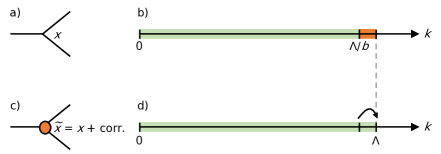
To keep track of the terms contributing to the solution it is helpful to employ a graphical language that is inspired by scalar Feynman diagrams (although it lacks the interpretation as particles and momenta) [24]. Each term of the perturbation series is represented as a directed graph . We only need very few graphical elements: external lines, internal lines connecting vertices, and a “sink” of internal lines representing the correlation function . Each vertex has one incoming line and outgoing lines [e.g., Fig. 2(a) for ]. A single () outgoing line represents the propagator while the correlation function [Fig. 2(d,e)] has only incoming lines (). The sum of outgoing wave vectors of each vertex equals the incoming wave vector , which is enforced by the -distribution in Eq. (15).
To construct the final graph from a bare initial vertex we iteratively either [Fig. 2(b)]
-
•
replace a line by the linear solution or
-
•
attach a vertex to one outgoing line (this line becomes the internal incoming line of the new vertex).
Finally, all intermediate lines need to end in an open dot, which joins exactly two lines so that the sum of their wave vectors vanishes [Fig. 2(c)]. This step implicitly performs the average over the noise and the open dot plus the two lines together represent the correlation function [Fig. 2(d)]. It should be easy to see that there are multiple ways to arrive at the same final graph . Section A shows how to calculate the multiplicity as the number of permutations in the construction of the graph. For example, the multiplicity of the graph Fig. 2(c) is because for each of the two steps there are two possibilities.
3.3 From graph to integral
The final graph can then be translated into one or several nested integrals . All internal lines connecting two vertices represent with the corresponding wave vector. All external outgoing lines represent fields with one exception: If there is exactly one outgoing line () then its wave vector is necessarily and it also represents . In the following, for the final graphs we use the convention that the single incoming wave vector is , outgoing wave vectors are with , and internal wave vectors are that will be integrated out. Each internal wave vector necessarily implies a corresponding loop in the graph. For example, reading the graph Fig. 2(c) from left to right leads to
| (18) |
and we need to integrate out to obtain the lowest-order correction to the bare propagator . The pre-factor is the multiplicity of the graph.
Summing over all distinct graphs with the same number of outgoing lines yields the “graphical corrections”
| (19) |
for the vertex functions. We emphasize that the integrals in general are functions of the outgoing wave vectors . To remain within the original model space (as defined by the function ), we have to reconstruct the functional form of the vertex neglecting terms involving higher orders of the wave vectors. The final step is to determine how the model parameters change due to these graphical corrections by comparing the coefficients on both sides of Eq. (19). While for simple vertex functions the can be read off, for functions that involve several outgoing wave vectors the problem can be cast as a system of linear equations (Sec. B).
3.4 Wilson’s shell renormalization
The arguably most common scheme to implement the procedure sketched in Fig. 1 is to consider an infinitesimal “shell” of wave vectors through setting and only consider contributions to linear order of . The first important consequence is that we only have to consider graphs with a single loop, and thus a single internal , since graphs with multiple loops are of higher order. Assuming that vertex functions are of the form , from Eq. (19) we thus find with quantifying the graphical one-loop corrections for due to the non-linearities. The next step is to restore the cut-off through rescaling, implying
| (20) |
to linear order. Wilson’s flow equations thus read
| (21) |
Figure 3 summarizes the procedure.
3.5 Handling the integrals
At this point we have to face the integral . The first step is to integrate over the internal frequency , which only involves the bare propagators. The generalization of Eq. (9) for the product of the bare propagators inside the loop reads
| (22) |
with the corresponding wave vector of the loop edge. Here, is the sign of within (remember that we set all external frequencies to zero). If all signs are equal then . For propagators and mixed signs one finds
| (23) |
with similar but more complicated expressions for propagators.
The integral over the internal wave vector is performed in spherical coordinates,
| (24) |
with polar angle , the surface area of a unit hypersphere in dimensions, and . Here, is the gamma function generalizing the factorial to non-integers. Useful angular integrals in the following are [25]
| (25) | |||
| (26) | |||
| (27) |
Finally,
| (28) |
for any function of the magnitude .
4 Illustrations
4.1 Model A/B: Wilson-Fisher fixed point
To demonstrate how this machinery works in practice we first turn to model A/B [Eq. (2)]. Let us see when becomes irrelevant, for which rescaling yields the scaling dimension and thus with . In dimensions the non-linear term is irrelevant and the Gaussian fixed point is attractive. This changes for with moving away from a small but non-zero initial . We will now determine where it flows to. Model A/B has one non-zero vertex [Fig. 4(a)], which implies that graphs can only be constructed from -vertices.

We start with the graph in Fig. 4(b), which contributes
| (29) |
to the propagator with multiplicity since there are three ways to connect two out of three lines. The integral becomes
| (30) |
with the static structure factor given in Eq. (9). From we find
| (31) |
expanding again for small . Plugging in , we can now read off the graphical corrections of the model parameters with intermediates (whence ) and
| (32) |
due to Fig. 4(b).
We now turn to the graph in Fig. 4(c). The multiplicity of this graph is: (possibilities to insert the new vertex) (remaining possibilities to insert a noise) (possibilities to insert a noise in the new vertex). Reading from left to right vertex, we have
| (33) |
leaving out the external lines (they are not part of the function ). We can immediately set inside the integral since also will only depend on . The frequency integral of then reads [cf. Eq. (22)]
| (34) |
Since the pre-factor in Eq. (33) is already we can let for the remaining terms inside the integral, which yields and thus
| (35) |
A quick look at Fig. 4(d) reveals that the first correction to is already a two-loop integral and thus of order with .
For the final flow equations we introduce the reduced “dimensionless” model parameters
| (36) |
leading to
| (37) |
through inserting their flow equations (21). Note how this choice removes the unknown exponents since with the scaling relations derived in Sec. 2.3 we find and . At this point the dimension is simply a number and not necessarily an integer. This freedom is exploited to introduce the small parameter with non-integer dimension close to the upper critical dimension at which the Gaussian fixed point becomes repulsive. The final flow equations then read
| (38) |
expressed in the reduced parameters. Besides the Gaussian fixed point () these equations admit another fixed point of order , the Wilson-Fisher (WF) fixed point located at and to linear order [26]. The resulting flow of the reduced parameters is plotted in Fig. 5. For this model, the perturbative approach thus has been successful since the non-linear parameter remains small and does not run off.
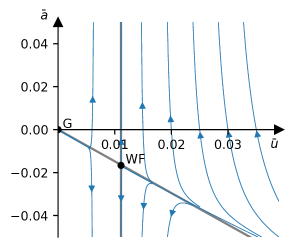
To understand the flow around WF, we define and measuring the distance to the critical point with new model parameters . The coupled linearized flow equations read
| (39) |
up to linear order of . This matrix has two eigenvalues. The first is and thus becomes irrelevant for . As a consequence, the flow of is repelled from G and flows towards WF along its eigenvector. The second eigenvector is so we identify its eigenvalue with . We expect the correlation length to diverge as with exponent . From the scaling dimensions (Sec. 2.3) we immediately find and thus . While strictly valid only close to , the expansion in can be improved systematically and there is ample evidence that the WF controls the critical behavior down to [27].
4.2 Burgers-KPZ equation
In a seminal paper Kardar, Parisi, and Zhang (KPZ) proposed that the equation
| (40) |
governs the non-equilibrium dynamics of a coarse-grained height field above a -dimensional substrate [6, 28]. In this context, is the surface tension smoothing the surface and determines the local growth rate along the surface normal. The field is not conserved and thus . Moreover, , implying scale-free growth with the roughness exponent determining whether the surface is smooth () or rough ().
Invariance of Eq. (40) under scaling yields the scaling relations
| (41) |
Importantly, Eq. (40) enjoys Galilean invariance through replacing together with describing an infinitesimal tilting of the surface. This symmetry implies that the coefficient cannot receive graphical corrections, [29].
Let us calculate the remaining corrections . The only non-zero vertex is given through . For the graph shown in Fig. 2(c) we have already calculated the frequency integral in Eq. (34). Plugging this result with into Eq. (18) leads to
| (42) |
To calculate this integral, we symmetrize and expand in powers of with . To lowest order the integrand reads
| (43) |
Performing the angular integrals [Eqs. (25) and (27)] and reading off leads to
| (44) |
Importantly, since the lowest order is this graph only corrects but does not generate a correction to , which remains zero. Here we have defined the sole dimensionless parameter .
Turning to the graph 2(e), now the noise does receive corrections through
| (45) |
Here something new has happened since the graph includes two correlation functions. The possible permutations of noise terms is described by Isserlis’ (or Wick’s) theorem and yields the additional multiplicity factor two. Comparing with the expression for [Eq. (8)], we read off the correction
| (46) |
for the noise strength . The flow equation for our single dimensionless model parameter reads
| (47) |
Plugging in the scaling relations for the and the graphical corrections [Eqs. (44) and (46)] leads to the closed flow equation [6]
| (48) |
for the non-linear coefficient. We recover the Gaussian fixed point at , which is attractive for and repulsive for . In dimensions there is a second perturbative fixed point at to lowest order in , which is connected to a dynamic phase transition (“roughening transition”). For a discussion, we refer to the literature, e.g. Ref. [30].
4.3 A neural network model
As the third and final example, we consider
| (49) |
with non-conserved noise (). This evolution equation has been derived recently in Ref. 31 for the evolution of a neural network (related to the famous Wilson-Cowan model [32]), where is a neural activity field. We have , , and . Hence, we now have to consider all graphs that can be constructed from both -vertices and -vertices, which are depicted in Fig. 6.

All corrections are at order , which immediately implies and we can set all external wave vectors to zero within the loop integral. For the propagator, the graph Fig. 2(c) contributes
| (50) |
and together with Fig. 4(b) we obtain . As before, we define dimensionless parameters
| (51) |
Similar to the KPZ model, no correction is generated and remains zero with diverging correlation length throughout.
Let us move on to . The integral of Fig. 6(a) is
| (52) |
with from Eq. (23). Since we set all external wave vectors to zero, reduces to a number. For propagators, the denominator contributes a factor so that the prefactor of all integrals is simply and the integrals are only distinguished by the products of and . In Table 1, we summarize all graphs together with their multiplicity and the signs. From this table, we can essentially read off the integration result for all further graphs, leading to333Note that for the second and third term of we find slightly different coefficients from Ref. [31].
| (53) |
The final flow equations read
| (54) | |||
| (55) |
for the two dimensionless non-linear parameters.
| figure | multiplicity | order | signs | |
|---|---|---|---|---|
| 2(e) | 2 | |||
| 2(c) | 4 | |||
| 4(b) | 3 | |||
| 6(a) | 4 | |||
| 6(b) | 8 | |||
| 6(c) | 6 | |||
| 6(d) | 12 | |||
| 4(c) | 18 | |||
| 6(e) | 12 | |||
| 6(f) | 24 | |||
| 6(g) | 6 | |||
| 6(h) | 12 | |||
| 6(i) | 12 | |||
| 6(j) | 8 | |||
| 6(k) | 16 |
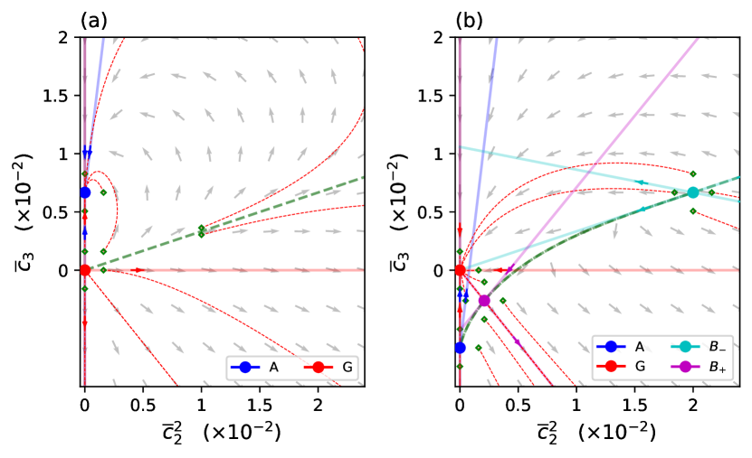
In Fig. 7, we plot the flow for two values of in the plane . The Gaussian fixed point at is attractive for and becomes repulsive for . For we find another perturbative fixed point at , which is attractive for and now governs the flow in the vicinity of . For , becomes repulsive and we now find two more perturbative fixed points from the quadratic equation [after eliminating by setting Eq. (54) to zero]
| (56) |
with solutions and and thus at and at . These fixed points require so that .
Starting from an initial point in the plane, there are two possible behaviors: either the flow runs into an attractive fixed point ( for and for ) or the flow runs off to infinity. This could be an artifact of the one-loop approximation (Ref. [31] finds numerical evidence for that this is indeed the case) or it indicates the existence of a strong-coupling fixed point that is not accessible in our perturbative approach. Both behaviors are delineated by a line, the separatrix.
To calculate the separatrices, we recast Eqs. (54) and (55) into a single differential equation , which can be solved through an appropriate change of variables and substitution. For it can be shown that the line is the separatrix. For , the separatrix was found by integrating the flow equations backward in time starting close to the saddle point and using linear analysis close to the unstable points and . While a comprehensive discussion of the implications is beyond the scope of these notes, this example demonstrates how fixed points shape the possible large-scale behavior.
5 Conclusions
We hope that we could show that calculating the one-loop flow equations for coarse-grained continuum models is conceptually not too difficult. Instead of focusing on (numerically) solving the evolution equations for a fixed set of parameters, these flow equations give insight into the possible large-scale behavior. Here we have restricted our attention to models up to order of the scalar field implying -vertices and -vertices, which already encompasses a large number of relevant models. Out of these we have presented three specific models, all of which have rather simple vertex functions. Going beyond and working with complex vertex functions that depend on several outgoing wave vectors is tedious and error prone, but can be tackled efficiently using symbolic computer algebra systems. A recent example is the extension of model B to active systems [13, 16]. As a companion to these notes, we have developed the package “REnormalization in STatistical physics and FLOW equations” (restflow)444You can access the code at https://github.com/us-itp4/restflow. implemented in python and based on sympy [33] that implements the techniques discussed here.
While numerical investigations of the macroscopic phase behavior in complex systems are indispensable, the flow equations yield complementary qualitative insights. Moreover, for driven systems governed by dynamics breaking detailed balance, many of the advanced numerical methods to improve sampling are not available and one has to resort to “vanilla” molecular dynamics. In this case renormalization offers a compelling alternative over computationally expensive simulations. The different phases are governed by the topology of fixed points in the space spanned by the model parameters. Critical fixed points with a diverging correlation length are of particular interest. In model A/B, we had to tune (typically related to the temperature) to reach the fixed point, which implies that it indeed corresponds to a critical point in the phase diagram. The other two models exhibit scale-free behavior throughout their parameter space.
Truncating at one-loop can introduce artifacts, e.g. the absence of a finite fixed point in the KPZ model for [30]. A compelling perspective is to adapt recent advances in the calculation of scalar Feynman graphs [24], such as master integrals and using that Feynman integrals obey differential equations [34], to statistical physics models and to move beyond one-loop graphs.
Appendix A Calculation of multiplicity for one-loop graphs

To calculate the multiplicity of a given one-loop graph , we cut the correlation function and arrange the vertices into a tree. Each edge ends in either: another vertex (black dot), a noise term (crossed dot), or nothing. For each vertex , the number of possible permutations of these three symbols is
| (57) |
with the number of outgoing edges, the number of black dots, and the number of crossed dots. The graph multiplicity is .
As an example, let us consider the graph Fig. 8(a), which has three vertices in total. Its tree is shown in Fig. 8(b). In Fig. 8(c-e), we have isolated the vertices and their edges. Fig. 8(c) has , , and with . Fig. 8(d) has , , and with . Fig. 8(e) has , , and with . Multiplying the number of permutations, we obtain .
Appendix B Reconstructing vertex functions
Given the model parameters , let us assume that we have calculated the sum of the one-loop graph integrals. We focus on a 2-vertex with scalar product but the following scheme extends to higher vertices. As already mentioned, we assume that is linear in the model parameters. Since vertex functions are polynomials, we expand in the monomial basis with constant coefficients . We expand the integral in the same basis. Using the definition of yields
| (58) |
and thus by comparing the basis coefficients
| (59) |
for all . This is a linear system of equations for the graphical corrections determined by the and the vertex structure encoded in the coefficients .
References
- [1] A. J. Archer and M. Rauscher, Dynamical density functional theory for interacting Brownian particles: Stochastic or deterministic?, J. Phys. A: Math. Gen. 37(40), 9325 (2004), 10.1088/0305-4470/37/40/001.
- [2] K. G. Wilson, The renormalization group and critical phenomena, Rev. Mod. Phys. 55(3), 583 (1983), 10.1103/RevModPhys.55.583.
- [3] P. C. Hohenberg and B. I. Halperin, Theory of dynamic critical phenomena, Rev. Mod. Phys. 49(3), 435 (1977), 10.1103/RevModPhys.49.435.
- [4] S.-k. Ma and G. F. Mazenko, Critical dynamics of ferromagnets in 6 - dimensions: General discussion and detailed calculation, Phys. Rev. B 11(11), 4077 (1975), 10.1103/PhysRevB.11.4077.
- [5] D. Forster, D. R. Nelson and M. J. Stephen, Large-distance and long-time properties of a randomly stirred fluid, Phys. Rev. A 16(2), 732 (1977), 10.1103/PhysRevA.16.732.
- [6] M. Kardar, G. Parisi and Y.-C. Zhang, Dynamic Scaling of Growing Interfaces, Phys. Rev. Lett. 56(9), 889 (1986), 10.1103/PhysRevLett.56.889.
- [7] F. Caballero, C. Nardini, F. van Wijland and M. E. Cates, Strong Coupling in Conserved Surface Roughening: A New Universality Class?, Phys. Rev. Lett. 121(2), 020601 (2018), 10.1103/PhysRevLett.121.020601.
- [8] A. Díaz-Guilera, Dynamic Renormalization Group Approach to Self-Organized Critical Phenomena, Europhys. Lett. 26(3), 177 (1994), 10.1209/0295-5075/26/3/004.
- [9] S. Mishra, R. Aditi Simha and S. Ramaswamy, A dynamic renormalization group study of active nematics, J. Stat. Mech. 2010(02), P02003 (2010), 10.1088/1742-5468/2010/02/P02003.
- [10] J. Toner and Y. Tu, Long-range order in a two-dimensional dynamical XY model: How birds fly together, Phys. Rev. Lett. 75(23), 4326 (1995), 10.1103/PhysRevLett.75.4326.
- [11] J. Toner and Y. Tu, Flocks, herds, and schools: A quantitative theory of flocking, Phys. Rev. E 58(4), 4828 (1998), 10.1103/PhysRevE.58.4828.
- [12] A. Gelimson and R. Golestanian, Collective Dynamics of Dividing Chemotactic Cells, Phys. Rev. Lett. 114(2), 028101 (2015), 10.1103/PhysRevLett.114.028101.
- [13] F. Caballero, C. Nardini and M. E. Cates, From bulk to microphase separation in scalar active matter: A perturbative renormalization group analysis, J. Stat. Mech. 2018(12), 123208 (2018), 10.1088/1742-5468/aaf321.
- [14] A. Cavagna, L. Di Carlo, I. Giardina, L. Grandinetti, T. S. Grigera and G. Pisegna, Dynamical Renormalization Group Approach to the Collective Behavior of Swarms, Phys. Rev. Lett. 123(26), 268001 (2019), 10.1103/PhysRevLett.123.268001.
- [15] S. Mahdisoltani, R. B. A. Zinati, C. Duclut, A. Gambassi and R. Golestanian, Nonequilibrium polarity-induced chemotaxis: Emergent Galilean symmetry and exact scaling exponents, Phys. Rev. Research 3(1), 013100 (2021), 10.1103/PhysRevResearch.3.013100.
- [16] T. Speck, Critical behavior of active Brownian particles: Connection to field theories, Phys. Rev. E 105(6), 064601 (2022), 10.1103/PhysRevE.105.064601.
- [17] U. C. Täuber, Renormalization group: Applications in statistical physics, Nucl. Phys. B 228, 7 (2012), 10.1016/j.nuclphysbps.2012.06.002.
- [18] N. Goldenfeld, Lectures on Phase Transitions and the Renormalization Group, No. v. 85 in Frontiers in Physics. Addison-Wesley, Advanced Book Program, Reading, Mass (1992).
- [19] U. C. Täuber, Critical Dynamics: A Field Theory Approach to Equilibrium and Non-Equilibrium Scaling Behavior, Cambridge University Press, Cambridge, 10.1017/CBO9781139046213 (2013).
- [20] M. Doi, Second quantization representation for classical many-particle system, J. Phys. A: Math. Gen. 9(9), 1465 (1976), 10.1088/0305-4470/9/9/008.
- [21] L. Peliti, Path integral approach to birth-death processes on a lattice, J. Phys. France 46(9), 1469 (1985), 10.1051/jphys:019850046090146900.
- [22] P. C. Martin, E. D. Siggia and H. A. Rose, Statistical Dynamics of Classical Systems, Phys. Rev. A 8(1), 423 (1973), 10.1103/PhysRevA.8.423.
- [23] H.-K. Janssen, On a Lagrangean for classical field dynamics and renormalization group calculations of dynamical critical properties, Z. Phys. B 23(4), 377 (1976), 10.1007/BF01316547.
- [24] S. Weinzierl, Feynman Integrals (2022), arXiv:2201.03593.
- [25] I. S. Gradshteyn and I. M. Ryzhik, Table of integrals, series, and products, In Table of Integrals, Series, and Products, p. 395. Academic press (2014).
- [26] K. G. Wilson and M. E. Fisher, Critical Exponents in 3.99 Dimensions, Phys. Rev. Lett. 28(4), 240 (1972), 10.1103/PhysRevLett.28.240.
- [27] J. Le Guillou and J. Zinn-Justin, Accurate critical exponents from the -expansion, J. Physique Lett. 46(4), 137 (1985), 10.1051/jphyslet:01985004604013700.
- [28] K. A. Takeuchi, An appetizer to modern developments on the Kardar–Parisi–Zhang universality class, Physica A 504, 77 (2018), 10.1016/j.physa.2018.03.009.
- [29] E. Medina, T. Hwa, M. Kardar and Y.-C. Zhang, Burgers equation with correlated noise: Renormalization-group analysis and applications to directed polymers and interface growth, Phys. Rev. A 39(6), 3053 (1989), 10.1103/PhysRevA.39.3053.
- [30] E. Frey and U. C. Täuber, Two-loop renormalization-group analysis of the Burgers–Kardar-Parisi-Zhang equation, Phys. Rev. E 50(2), 1024 (1994), 10.1103/PhysRevE.50.1024.
- [31] L. Tiberi, J. Stapmanns, T. Kühn, T. Luu, D. Dahmen and M. Helias, Gell-Mann–Low Criticality in Neural Networks, Phys. Rev. Lett. 128(16), 168301 (2022), 10.1103/PhysRevLett.128.168301.
- [32] H. R. Wilson and J. D. Cowan, Excitatory and Inhibitory Interactions in Localized Populations of Model Neurons, Biophysical Journal 12(1), 1 (1972), 10.1016/S0006-3495(72)86068-5.
- [33] A. Meurer, C. P. Smith, M. Paprocki, O. Čertík, S. B. Kirpichev, M. Rocklin, Am. Kumar, S. Ivanov, J. K. Moore, S. Singh, T. Rathnayake, S. Vig et al., SymPy: Symbolic computing in Python, PeerJ Comput. Sci. 3, e103 (2017), 10.7717/peerj-cs.103.
- [34] J. M. Henn, Multiloop Integrals in Dimensional Regularization Made Simple, Phys. Rev. Lett. 110(25), 251601 (2013), 10.1103/PhysRevLett.110.251601.