Feature Selection for Forecasting

Abstract

This work investigates the importance of feature selection for improving the forecasting performance of machine learning algorithms for financial data. Artificial neural networks (ANN), convolutional neural networks (CNN), long-short term memory (LSTM) networks, as well as linear models were applied for forecasting purposes. The Feature Selection with Annealing (FSA) algorithm was used to select the features from about 1000 possible predictors obtained from 26 technical indicators with specific periods and their lags. In addition to this, the Boruta feature selection algorithm was applied as a baseline feature selection method. The dependent variables consisted of daily logarithmic returns and daily trends of ten financial data sets, including cryptocurrency and different stocks. Experiments indicate that the FSA algorithm increased the performance of ML models regardless of the problem type. The FSA hybrid machine learning models showed better performance in 10 out of 10 data sets for regression and 8 out of 10 data sets for classification. None of the hybrid Boruta models outperformed the hybrid FSA models. However, the BOR-CNN model performance was comparable to the best model for 4 out of 10 data sets for regression estimates. BOR-LR and BOR-CNN models showed comparable performance with the best hybrid FSA models in 2 out of 10 datasets for classification. FSA was observed to improve the model performance in both better performance metrics as well as a decreased computation time by providing a lower dimensional input feature space.

1 Introduction

After the financial crisis of 2008 and its effect on investors, institutions, academia, and governments, cryptocurrencies have gradually received attention as a resource of alternative revenue. Cryptocurrency is one of the most important investment tools that shows highly speculative behavior in the financial market. Over the last few years, especially due to the COVID-19 pandemic, cryptocurrency and stock investments have received great interest from investors worldwide. The large increase in the trading volume of the investment tools made it more important to forecast the future value of the assets.

Financial time series are ambiguous and have a nonlinear dynamic structure and chaotic movements, making forecasting quite difficult. Stock market and cryptocurrency indices depend on numerous macroeconomic factors such as political changes, the general outlook of the economy, investors’ expectations as well as investment preferences and movements in other indices, making index forecasting quite difficult but also attractive. Many studies use conventional methods and machine learning algorithms such as artificial neural networks (ANN), support vector machines (SVM), naive Bayes (NB), and random forest (RF) to address the issue.

According to the efficient-market hypothesis proposed by Fama, (1970), stock prices are essential information and can be forecast based on trading data. Efficient market strategies should be developed to make safe and valid forecasts for stock index movements or other financial assets (Leung et al.,, 2000). Such market strategies protect investors from potential market risks and speculators. According to the efficient-market hypothesis, stock market indices can be effectively defined, and future forecasts can be made using trading data sets. This makes as much sense as the reflection of the political situation of a country or the public image of a firm on stock prices. Therefore, if we efficiently process information based on stock prices or stock index data using appropriate methods or algorithms, we can then forecast stock prices and trends. It can be said that all of the above-mentioned also apply to cryptocurrencies due to similar behavior.

Over the years, numerous methods have been developed to forecast stock prices or returns and cryptocurrency prices or returns. One of the earliest of these methods is the classical regression analysis. Stock index data sets are pre-processed because they have a chaotic behavior and contain uncertainties and nonlinear relationships, resulting in information loss. Therefore, machine learning algorithms have recently been more popular than conventional methods (regression analysis, discriminant analysis, statistical methods, etc.) for financial time series forecasting.

The new research direction began with McCulloch and Pitts, (1943) in the field of artificial neural networks. ANN theory was formulated quickly by Hebb, (1949) and the Perceptron (Rosenblatt,, 1958) in the next years. The research on artificial neural networks did not show much progress for a while, especially after Minsky and Papert, (1969). The reason is that computers did not have enough power to produce high-accuracy results. The next period of rapid growth for neural networks was due to the reinvention of the back-propagation algorithm by Rumelhart et al., (1986), which made the ANN a prominent actor in this field of research. Algorithms such as artificial neural networks and support vector machines are commonly used because they do not make many restrictive assumptions on the data. Artificial neural networks (Hassan et al.,, 2007; Kara et al.,, 2011; Kimoto et al.,, 1990; Olson and Mossman,, 2003; Wei,, 2016) and support vector machines (Hsu et al.,, 2009; Huang et al.,, 2005; Kumar and Thenmozhi,, 2006) have yielded successful results.

The non-sequential data type used in Multi-Layer Perceptron (MLP) models and temporal dependent structure of the input data made the Recurrent Neural Network (RNN) models more convenient compared to the MLPs in financial time series forecasting. Kamijo and Tanigawa, (1990) applied the RNN model by using the Tokyo Stock Exchange data and obtained a 93.8% accuracy. The vanishing gradient problem specific to deep neural networks, as well as RNNs was addressed by the introduction of Long-Short Term Memory (LSTM) networks. Cho et al., (2014) and Di Persio and Honchar, (2017) applied LSTM with dropout to the Google stock prices. Some similar results can be found in Bao et al., (2017); Pawar et al., (2019); Zhao et al., (2017).

The main objective of this research is to investigate whether feature selection methods can be used to improve the forecasting accuracy of different machine learning algorithms for stock and cryptocurrency returns.

2 Related Work

Statistical models make some simplifying assumptions to be able to obtain some theoretical guarantees and thus have a simple structure and potentially lover performance compared to machine learning techniques. Machine learning models are more general, make fewer simplifying assumptions, and offer better model-fitting capabilities. Due to these reasons, techniques such as ML and deep learning created a new research direction in the financial literature (Fang et al.,, 2021). To forecast the future value of financial assets and find the reason for these assets’ behavior, numerous machine learning (ML) techniques were employed, such as SVM (Akyildirim et al.,, 2021), Support Vector Regression (SVR) (Kara et al.,, 2011), Random Forest (RF) (Patel et al., 2015a, ), and convolutional neural networks (CNN) (Tsantekidis et al.,, 2017). These works show that it is possible to use ML techniques to make more accurate forecasts and as alternative approaches to conventional techniques for investigating the behavior of financial assets. Nousi et al., (2019) applied several ML techniques such as single hidden layer feed-forward neural network, MLP, autoencoders, and bag-of-features algorithms to forecast the mid-price movement of the stock price. The results indicated that the mentioned ML techniques could forecast price movement. Shah et al., (2019) organized the stock price prediction techniques into four categories, namely statistical methods, pattern recognition, machine learning, and sentiment analysis. The financial time series forecasting problems can also be categorized into classification and regression problems. According to Patel et al., 2015b , the most widely used two techniques are ANN and SVR, which are supervised methods, while the unsupervised methods are less popular. A review of machine learning techniques for financial time series forecasting is presented in Henrique et al., (2019). The authors note that ANN seems to be the most popular ML technique in the financial time series literature.

Machine learning techniques like ANN, SVM, or decision trees can learn the trends of stock or cryptocurrency returns from historical data. They can provide significant information and analysis of historical returns. Bernal et al., (2012) applied an RNN called Echo State Network to forecast the S&P 500 stock prices using a couple of technical indicators such as moving averages as an input. The proposed technique in this study outperformed the Kalman filter as a benchmark based on test error statistics. The authors used 50 different financial data sets and reported the forecasting results. Ballings et al., (2015) compared the performance of classifiers such as ANN, Logistic Regression (LR), SVM, and k-nearest neighbor with AdaBoost and RF. They reported the Random Forest algorithm as the best option to forecast the stock price movement based on area under curve (AUC) and cross-validation metrics. Borges and Neves, (2020) looked at the most traded volume of 100 cryptocurrency prices from Binance with a 1-minute frequency, using the returns and some technical indicators as input. The authors regarded it as a classification problem, applying logistic regression, random forest, support vector machine, gradient tree boosting, and an ensemble of mentioned algorithms. Chen et al., (2020) used 5 min and daily bitcoin price index and trading price in USD to measure the LR, Linear discriminant analysis (LDA), RF, ANN, LSTM, and XGBoost algorithm performances. Four Blockchain information variables, trading variables, Google trend search volume indexes, and gold spot prices were used as input features. The authors reported that the LSTM model has the best accuracy level of 67% for 5 min data and LR and LDA have the best accuracy level of 65% for daily data. Sun et al., (2020) used 42 cryptocurrencies’ daily data and applied light gradient boosting machine (GBM), SVM, and RF to forecast the movement of the prices. Sun et al., (2020) reported that light GBM outperformed other ML techniques based on accuracy performance metrics.

LSTM networks have been applied in numerous studies in the financial forecasting literature. Lahmiri and Bekiros, (2019) discussed the research problem as a regression by using the LSTM and generalized regression neural network (GRNN). Daily Bitcoin, Digital Cash, and Ripple prices were used as input features in this study.Lahmiri and Bekiros, (2019) reported that LSTM had a significantly better performance than GRNN. Smuts, (2019) applied LSTM using an input set that contains telegram chat groups talking for Bitcoin, Google trends, price volumes, and trading of bitcoin and Ethereum. Results showed that telegram data is a better predictor for bitcoin, however, Google trend data is better for ethereum, especially in the weekly periods. Di Persio and Honchar, (2017) reached the level of accuracy of 72% on Google stock price by comparing different RNN model performances such as LSTM, gated recurrent unit (GRU), and a basic RNN. Roondiwala et al., (2017) also applied an LSTM to forecast Nifty prices by using the open, high, low, and close values as input variables. RMSE was used as a performance metric. McNally et al., (2018) used the Bitcoin prices’ open, close, high, and low values and the hash and difficulty rate of the blockchain for different periods to construct an input set. The problem was considered a regression and classification, and LSTM and Bayesian recurrent neural networks were used as learning algorithms. The authors reported that 20 days are the best period for RNN and 100 days for LSTM. Fang et al., (2021) reported that the mid-price movement of Bitcoin could be predictable at an accuracy level of 78% using LSTM.

Han et al., (2020) used a nonlinear autoregressive with exogenous variable (NARX) technique for predicting Bitcoin return in USD on a daily frequency. Bitcoin return was also used as an input feature, and the author reported that the NARX model could predict the trend but not breaks. Atsalakis et al., (2019) proposed a hybrid neuro-fuzzy controller (PATSOS) model to forecast the Bitcoin, Ethereum, Ripple, and Litecoin prices, considering the problem both as classification and regression. PATSOS was observed to have a significantly better forecast than other selected benchmark models in that study. Especially PATSOS predicted returns significantly better than the buy/hold strategies that are based on the predicted sign of the selected technical indicators. Basher and Sadorsky, (2022) looked at forecasting Bitcoin price movement for predicting a possible trend in a specific period, and for planning asset allocation using this information. The research investigated the importance of cryptocurrency forecasting of different input variables such as inflation rate, interest rate, and market volatility. The authors applied tree-based machine learning techniques to forecast the direction of Bitcoin prices and reported accuracy levels between 75% and 80%.

Feature selection is an important problem for financial time series forecasting, especially in social sciences. An effective feature selection process can improve the generalization ability of the forecasting models by removing many irrelevant features from the input space. However, this problem has not received enough attention in the financial literature. According to Niu et al., (2020) there are three types of feature selection methods: (1) embedded methods; (2) filter-based methods; (3) wrapper methods. Each of these methods has advantages and limitations and can be applied to financial time series forecasting problems.

Tyralis and Papacharalampous, (2017) proposed a feature selection model based on a Random Forest algorithm to suggest an optimal set of input variables. The authors used two different time series datasets and compared the results with standard benchmark models. As a result, the RF model for feature selection showed better performance when using a few short-lag input features. Valente and Maldonado, (2020) proposed an approach for time series forecasting by adapting the SVR for feature selection. The authors used an ARIMA model with feature selection to forecast the energy load. 1700 lags were used for high-frequency data and less than 400 lags were used for daily data. The proposed methodology showed slightly better performance compared to selected conventional techniques such as ARIMA models. Niu et al., (2020) proposed a two-stage multi-objective wrapper-based feature selection to determine the optimal input space for deep learning models. MAE, MSE, and MAPE statistics were used for evaluating the model performance. The authors reported that the proposed model for feature selection significantly improved the forecasting performance. Ghosh et al., (2022) proposed an ensemble feature selection algorithm to forecast the stock price using the national stock exchange data in India by assessing the COVID-19 effect. Spot prices, market sentiment, sectoral outlook, crude price volatility, and exchange rate volatility features were used in this study. The authors proposed a structural model to determine the effect of selected variables, comprising Boruta and Regularized Random Forest algorithms. Regularized greedy forest and deep neural network algorithms were used with PCA and autoencoders. It was indicated that the importance of the input features depends on the particular stock and the period under consideration.

The main contribution of this paper is to study the importance of feature selection for the forecasting problem using ML algorithms, in both classification and regression settings. It uses ten different financial time series data sets, including cryptocurrencies and stock markets. This study investigates the predictability of the selected stock and cryptocurrency return, which means profitability, based on ML techniques with and without feature selection as a regression problem, and the binary buy and sell strategies based on the same techniques as a classification problem. The study evaluates several ML techniques, namely Logistic Regression (LR), artificial neural networks (ANN), convolutional neural networks (CNN), and long short-term memory (LSTM), after applying the feature selection with annealing (FSA) Barbu et al., (2016) and the Boruta algorithm Ghosh et al., (2022) as a benchmark method.

3 Data Preparation

In this research, three different types of information were used from the original data.

• Historical prices from Yahoo finance, using the Python finance API. The collected data contains the date, opening price, high price, low price, closing price, adjusted closing price, and volume information from a specific date interval depending on the data availability. The dataset information is presented in Table 1.

• Technical indicators: four classes of technical indicators were used, namely momentum, volume, volatility, and trend indicators. A total of 26 technical indicators were gathered using the Python technical analysis library (TA-Lib). While calculating the technical indicators, six different periods were used: 2, 4, 8, 16, 32, and 64 for each of the indicators. A total of 185 features were obtained from these calculations.

• Lag operator: The first five lag (1, 2, 3, 4, 5) periods were used for all calculated indicators and added to the feature pool. A total of 925 features were obtained using this operator.

Using these three sources, a feature pool was constructed from the historical stock and cryptocurrency data to apply feature selection algorithms and remove the irrelevant features from the model.

Table 1: Dataset information

Data	Code	Start date	End date	# Observations	# Features
Tether	TTH	3/24/2018	4/21/2022	1477	1105
Ethereum	ETH	11/09/2017	05/17/2022	1513	1105
Bitcoin	BTC	04/21/2017	04/21/2022	1690	1105
Ripple	RPL	03/24/2018	05/31/2022	1525	1105
Tesla	TSL	04/21/2017	04/21/2022	1112	1105
Nasdaq	NSDQ	11/28/2017	05/16/2022	1123	1105
Nikkei225	NKK	05/17/2017	05/17/2022	1022	1105
New York Stock Exc.	NYSE	11/28/2017	05/16/2022	1085	1105
Standard &Poors 500	S&P500	05/17/2017	05/16/2022	1121	1105
Gold	GLD	11/28/2017	05/16/2022	1101	1105

After constructing the input feature pool, the datasets were prepared for analysis by conducting data preprocessing. This involved removing some rows (samples) from data that contained missing or infinite values obtained during the feature calculation process. Thus, different numbers of observations were obtained for each dataset. There also exist differences between stock and cryptocurrency data samples in terms of hours of operation and data availability. A total of 1105 features were obtained for the input feature space, as presented in Table 1.

The input dataset was standardized for both feature selection and forecasting techniques. We considered two prediction targets, a regression, and a classification target. Logarithmic returns were used as the target for the regression problem. For classification, a binary output (Eq. 1.) was used to represent the up and down movement of the logarithmic returns. The up and down movement was coded as $\{-1,1\}$ for FSA and $\{0,1\}$ for the forecasting models.

$$y_{t}=\begin{cases}1,\text{ if }return_{t}>return_{t-1}\\ -1,\text{ else }\end{cases}$$ (1)

We considered the forecasting problem of predicting the target at time $t$ from the input features at time $t-3$. We observed that when trying to predict the target at time $t$ from the input features at time $t$ or $t-1$ a very high accuracy and high $R^{2}$ values were obtained for regression, which means that the research problem was too simple. This is why in the end we settled on the forecasting problem of predicting the target at time $t$ from the features at time $t-3$, where a lower accuracy and higher MSE values were obtained, but more reliable results.

The data was partitioned in $70\%$ for training and $30\%$ for testing for all models.

4 Problem and methodology

Financial time series forecasting is an important problem and numerous studies address it using statistical methods and machine learning techniques. However, while many published papers focus on improving the classification accuracy or decreasing the error for the regression problems they ignore the feature selection problem, which would help select the relevant features from a larger pool and help construct models with better generalization. We investigate the effect of feature selection on the performance of the selected techniques to forecast the financial time series. The methodology used in this paper is presented in Fig. 1.

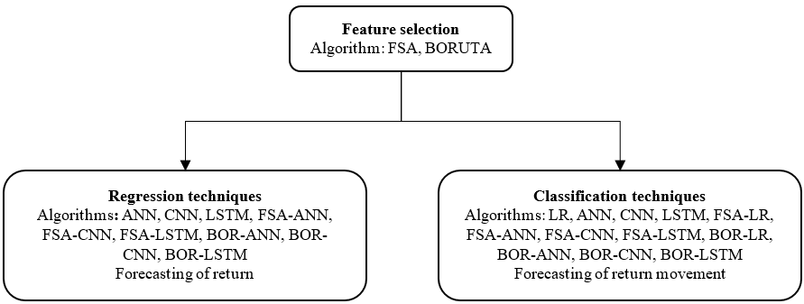
Figure 1: Research methodology.

4.1 Feature selection methodology

Feature selection is the problem of finding the relevant features in building a model, which can help improve generalization while reducing the computation time and the cost associated with obtaining the data. For that reason, we decided to apply the Feature Selection with Annealing (FSA) method Barbu et al., (2016) due to its good feature selection capabilities. FSA is a highly efficient feature selection algorithm that besides efficiency has statistical true feature recovery and convergence guarantees, is easy to implement, and can handle nonlinearity to a certain extent. In FSA, the feature selection problem is formulated as a constrained optimization problem,

$${\boldsymbol{\beta}}=\mathop{\rm argmin}_{|\{j,\beta_{j}\not=0\}|}L({\boldsymbol{\beta}})$$ (2)

where $k$ is the number of relevant features (a given parameter), and the loss function $L(\beta)$ is differentiable with respect to $\beta$. The key ideas in the algorithm design are a) using an annealing plan to lessen the greediness in reducing the dimensionality from $p$ (the initial number of features) to $k$ (desired number of features) and b) gradually removing the most irrelevant features to facilitate computation. The parameter ranges used in experiments are presented in Table 2.

Table 2: FSA parameter values.

Parameters	Levels
Learning rate $\eta$	0.01-0.1
Annealing parameter $\mu$	0,1,20,50,100,300,500,1000
Number of epochs	50, 100, 200, 300, 500

We also implemented a Boruta feature selection process Ghosh et al., (2022) as a benchmark model to evaluate and compare the FSA algorithm performance. Boruta is an ensemble feature selection algorithm that uses a Random Forest together with a feature importance measure to select the relevant feature from the input space Kursa and Rudnicki, (2010). We used the existing scikit-learn implementation of the Boruta algorithm available at https://github.com/scikit-learn-contrib/boruta_py.

4.2 Forecasting methodology

This section gives an overview of the machine learning methods that will be used to forecast the financial time series in this paper, namely logistic regression, artificial neural network (ANN), convolutional neural network (CNN), and long short term memory (LSTM).

4.2.1 Logistic regression

Logistic regression is a popular technique to model the probability of discrete (i.e. binary or multinomial) outcomes, indicated by the class label. Logistic regression is a multiple regression model with a dependent variable $y\in\{0.1\}$ for binary classification or $y\in\{0.1,…,n\}$ for multinomial classification. The dependent variable is predicted from the input feature vector $\ x=(x_{1},...,x_{p})\in\mathbb{R}^{p}$. The logistic regression model can be expressed as follows,

$$\log\frac{P(y=1|\mathbf{x})}{1-P(y=1|\mathbf{x})}\ ={\boldsymbol{\beta}}_{0}+{\boldsymbol{\beta}}_{1}x_{1}+\dots+{\boldsymbol{\beta}}_{p}x_{p}$$ (3)

Learning the parameters ${\boldsymbol{\beta}}=(\beta_{0},...,\beta_{p})$ is done by optimization of the negative log-likelihood loss function, which can also have an $L_{1}$ or $L_{2}$ penalty term to improve generalization. We used the $c$ parameter, which represents the inverse of regularization strength, and smaller $c$ values specify stronger regularization.

The Python scikit-learn library is used for the LR implementation and the parameter levels that are used in the study are given in Table 3.

Table 3: Logistic regression (LR) parameter levels.

Parameters	Levels
Penalty	L1-L2
Inverse regularization strength parameter $c$	0.1, 0.3, 0.5, 1
Solver	lbfgs, liblinear
Tolerance	0.0001

4.2.2 Artificial neural network

ANN has been commonly used for forecasting purposes of stock or cryptocurrency prices or the movement of these values. MLP’s flexible structure and their success in many studies, such as Kara et al., (2011); Patel et al., 2015a , indicate that MLP might have an advantage compared to traditional statistical models. A feed-forward neural network model is used in this study with different numbers of hidden layers and number of neurons.

The log sigmoid is used for the output layer, and tangent sigmoid and rectified linear unit (ReLU) functions are used for the hidden layer neurons as activation functions. Stochastic gradient descent and ADAM optimization algorithms are used for training the ANN. The loss functions are the MSE loss for regression and the binary cross-entropy loss for classification problems. A comprehensive set of parameter combinations in the ranges presented in Table 4 have been explored to determine the best combination. The Python Keras library was used for the implementation of the ANN.

Table 4: ANN parameter levels.

Parameters	Levels
Learning rate ($\eta$)	0.01-0.1
Momentum constant (c)	0.1-0.9
Number of epochs	50, 100, 200, 500
Number of hidden layers	1, 2, 3
Number of neurons for each hidden layer	10, 20, 50, 100
Activation function	ReLU, tanh, sigmoid
Optimizer	SGD, ADAM

4.2.3 Convolutional neural network

CNN is one of the most popular machine learning (neural network) techniques, performing well on different regression or classification problems such as Qian et al., (2020). Each neuron receives an input signal from the input feature space and operates as in ANN. CNN structure lets the connection with locally sharing weights and determining the local features effectively(Zhang et al.,, 2021). One of the main differences between ANN and CNN is the field of usage. CNN has generally used pattern recognition within the images. CNN has a convolutional layer, pooling layer, and output layer, and the main components are convolutional and pooling layers. The convolutional layer extract local features, and the pooling layer reduce the dimension of the parameter in addition to minimizing the over-fitting possibility (Zhang et al.,, 2021). The inputs for the networks are the time series data features like a signal. Python Keras library is used for the implementation of CNN. CNN layer information was presented in Table 5.

Table 5: CNN parameter levels.

Parameters	Levels
Convolution layers	Conv1D layer
Number of hidden layers	1,2,3
Number of hidden neurons	20, 30, 40, 50
Kernel size	$2,3,4,5,6$
Pooling layer	MaxPooling1D Layer
Pool size/Stride	2/ 1
Activation function	ReLU, tanh, sigmoid
Optimizer	SGD, ADAM

4.2.4 Long short-term memory

The LSTM network developed by Hochreiter and Schmidhuber, (1997) is an extension of Recurrent Neural Networks, redesigned to handle the vanishing gradient problem in recurrent neural networks. LSTM consists of a memory cell to store the information coming from inputs through the three gates, namely the input gate $i(t)$, the forget gate $f(t)$, and the output gate $c(t)$, which updates the information. LSTM can be formulated as follows (Chen et al.,, 2020):

$$\begin{split}X&=\begin{bmatrix}x_{t}\\ h_{t-1}\end{bmatrix}\\ f_{t}&=\delta(W_{f}X+b_{f})\\ i_{t}&=\delta(W_{i}X+b_{i})\\ c_{t}&=\delta(W_{0}X+b_{0})\\ \end{split}$$ (4)

where $x_{t}$ and $h_{t}$ are the input and respectively the hidden state at time $t$, $W_{j},W_{i}$ and $W_{0}$ are the weight matrices of the corresponding components, $b_{f},b_{i},b_{0}$ are the corresponding bias parameters, and $\delta$ is the activation function.

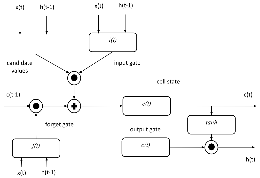
Figure 2: LSTM architecture Graves, (2013).

We adopt LSTM as a promising machine learning method for predicting the future based on past information without assuming any noise form. Most importantly, LSTM could capture possibly nonlinear features behind the time series. The hyper-parameters of the LSTM model include the number of layers $L$ and the number of training epochs $E$. Note that since a linear structure is a special case of a feed-forward neural network when armed with a linear transformer, one should expect that LSTM performs at least as well as MLP. The Python Keras library is used for the implementation.

Table 6: LSTM parameter levels.

Parameters	Levels
Activation function	ReLU, tanh, sigmoid
Optimizer	SGD, ADAM
Number of hidden layers	1, 2
Number of hidden neuron	10, 20, 30, 40, 50
Number of training epochs	50
Dropout rate	0.2,0.3

4.3 Evaluation criteria

The above ML regression and classification techniques were used to forecast on the financial time series data introduced in Section 3. During feature selection, the MSE loss function was used for the regression problem, and the binary cross entropy loss function was used for the classification problems. To evaluate and compare the model performance, the MSE metric was used for the regression problems, and accuracy and area under the ROC curve (AUC) metrics were used for classification, both based on the set aside test set.

5 Results

5.1 Feature selection results

As indicated before, the data is high dimensional, with different numbers of samples for each dataset due to the market condition and data availability. To reduce the high dimensionality, the FSA algorithm Barbu et al., (2016) with a linear model was applied to each data set, and the obtained results are presented in Tables 7 and 8 together with the parameter combinations that obtained those results. Parameters $\mu,s$, and $\eta$ are the most important parameters for the FSA algorithm. The number of relevant features is generally different for the regression and classification problems as well as the annealing parameter ($\mu$). The annealing parameters are usually $\mu=300$ except for the “Tether”, “Bitcoin” and “Ripple” data sets in both regression and classification and NKK for classification.

Table 7: Regression results using linear FSA.

Data	k	$\mu$	s	$\eta$	$N^{iter}$	MSE
TTH	10	10	0.01	0.01-0.01	300	0.121
ETH	30	300	0.01	0.01-0.01	300	26.21
BTC	30	200	0.001	0.1-0.1	300	21.42
RPL	30	100	0.01	0.01-0.01	300	35.73
TSL	30	300	0.01	0.005-0.01	300	14.64
NSDQ	40	300	0.01	0.1-0.1	300	2.268
NKK	60	300	0.01	0.01-0.01	300	1.526
NYSE	20	300	0.01	0.1-0.01	300	1.705
S&P500	25	300	0.01	0.01-0.001	300	1.711
GLD	40	300	0.01	0.01-0.01	300	0.927

FSA reduced the high dimensional feature space by more than 95% , achieving the same or higher accuracy results on the test set. The accuracy levels of FSA for each dataset are quite low, around 0.5, except for the Nasdaq data. The accuracy level on Nasdaq is 0.748, which is the best value for classification problems, as seen in Table 8.

Table 8: Classification results using linear FSA.

Data	k	$\mu$	s	$\eta$	$N^{iter}$	Accuracy
TTH	10	1000	0.01	0.3-0.01	300	0.501
ETH	30	300	0.01	0.01-0.01	300	0.512
BTC	35	1000	0.01	0.01-0.01	300	0.525
RPL	10	100	0.01	0.001-0.001	300	0.538
TSL	30	300	0.01	0.1-0.1	300	0.507
NSDQ	10	300	0.01	0.1-0.1	300	0.748
NKK	60	100	0.01	0.1-0.001	300	0.519
NYSE	10	300	0.01	0.1-0.01	300	0.499
S&P500	15	300	0.01	0.01-0.01	300	0.530
GLD	45	300	0.01	0.1-0.1	300	0.488

The Boruta feature selection method Ghosh et al., (2022), which is quite popular in the forecasting literature, was also evaluated and compared process with the FSA method. As seen in Table 9 the regression MSEs of the Boruta method are higher than FSA and accuracy values are lower than FSA.

Table 9: Results obtained by the Boruta feature selection method Ghosh et al., (2022).

	Regression		Classification
Data	Number of features	MSE	Number of features	Accuracy
TTH	82	0.361	13	0.498
ETH	15	34.46	67	0.401
BTC	12	24.82	88	0.467
RPL	19	43.04	66	0.451
TSL	14	20.80	28	0.434
NSDQ	28	2.901	15	0.705
NKK	6	1.905	17	0.423
NYSE	13	2.416	18	0.451
S&P500	18	1.857	20	0.412
GLD	14	1.406	117	0.428

5.2 Return forecasting

Three regression algorithms are tested on the ten financial time series data sets introduced in Section 3. The selected time series’ daily values were used to forecast the selected stocks’ returns, as well as cryptocurrency and gold prices. The MSE was used for model comparison, and the results are presented in Table 10. Paired $t$-test were used to compare the best result for each column (shown in bold with a star) with the other results. Results that are not significantly worse ($p>0.05$) than the best result are also shown in bold, representing the top performing group.

The null model that always predicts the average return on the training set was also evaluated as a baseline comparison. One can easily say that the FSA algorithm improved the forecasting performance in most cases. As seen in Table 10, at least one of the FSA based models is in the top performing group (bold) for all 10 datasets.

Table 10: Return forecasting. MSE values for the 10 datasets evaluated.

Model/Data	TTH	ETH	BTC	RPL	TSL	NSDQ	NKK	NYSE	S&P500	GLD
Null	0.178	26.25	17.53	34.63	18.26	2.42	1.519	1.813	1.532	1.164
ANN	0.177	26.20	17.50	34.62	18.26	2.428	1.515	1.780	1.550	1.165
CNN	0.177	26.18	17.49	34.63	18.29	2.418	1.516	1.800	1.532	1.138
LSTM	0.209	27.01	17.11*	35.99	18.44	2.435	1.713	1.944	1.673	1.206
FSA-ANN	0.177	26.17*	17.50	34.33*	18.18*	2.399*	1.509*	1.773*	1.517*	1.167
FSA-CNN	0.172	26.22	17.52	34.63	18.26	2.418	1.519	1.804	1.532	1.053*
FSA-LSTM	0.168*	26.98	17.12	35.99	18.39	2.431	1.719	1.938	1.679	1.207
BOR-ANN	0.177	26.68	17.71	34.98	18.29	2.417	1.520	1.821	1.691	1.165
BOR-CNN	0.178	26.81	17.54	34.63	18.22	2.418	1.527	1.805	1.531	1.162
BOR-LSTM	0.213	27.71	17.89	35.99	18.39	2.432	1.692	1.970	1.680	1.199

If we compare the FSA-based model performances to the other models, we see that at least one FSA-based model significantly outperformed all non-FSA models on 3 out of the 10 datasets (TTH, S&P500 and GLD). In contrast, the non-FSA models including the Boruta-based models never outperformed the FSA based models significantly.

The null model is in the top performing group on four datasets (RPL, TLS, NSDQ and NKK), which means that no model could improve the performance of the null model significantly on these datasets.

On the three remaining datasets (ETH, BTC and NYSE), FSA is in the top performing group together with some non-FS based models, but Boruta based models are not in the top performing group on these datasets.

In fact, examining the 6 datasets where the null model is not in the top performing group, we see that Boruta based models are not in the top performing group on any of these six datasets. Therefore FSA-based models significantly outperform Boruta-based models on these six datasets.

5.3 Forecasting the return movement

As stated before, four classification algorithms were applied to the ten financial time series datasets introduced in Section 3. Accuracy and AUC metrics are used for the model comparisons in classification. The experimental results are presented in Table 11-12. Again, a star represents the best model for each column and the models that are not significantly worse than the best model ($p>0.05$) are shown in bold.

Table 11: Return movement forecasting. Accuracy values for the 10 datasets evaluated.

Model/Data	TTH	ETH	BTC	RPL	TSL	NSDQ	NKK	NYSE	S&P500	GLD
LR	0.524	0.515	0.507	0.517	0.515*	0.743	0.515	0.539*	0.518	0.503
ANN	0.487	0.498	0.485	0.527	0.494	0.745	0.535	0.516	0.538	0.496
CNN	0.502	0.517	0.490	0.535*	0.513	0.740	0.527	0.526	0.526	0.495
LSTM	0.482	0.529	0.523*	0.528	0.490	0.523	0.522	0.498	0.525	0.530
FSA-LR	0.500	0.525	0.515	0.532	0.513	0.737	0.518	0.532	0.510	0.540*
FSA-ANN	0.486	0.535	0.523*	0.535*	0.513	0.734	0.528	0.526	0.525	0.528
FSA-CNN	0.490	0.521	0.515	0.527	0.508	0.747*	0.553*	0.529	0.525	0.528
FSA-LSTM	0.527*	0.558*	0.509	0.515	0.463	0.521	0.528	0.534	0.554*	0.502
BOR-LR	0.493	0.464	0.513	0.533	0.461	0.530	0.442	0.512	0.477	0.492
BOR-ANN	0.484	0.467	0.513	0.522	0.488	0.509	0.544	0.512	0.468	0.500
BOR-CNN	0.468	0.473	0.516	0.506	0.470	0.530	0.540	0.521	0.483	0.503
BOR-LSTM	0.470	0.513	0.495	0.503	0.505	0.532	0.453	0.454	0.521	0.479

In terms of accuracy, from Table 11 one can see that an FSA-based model significantly outperforms all non-FSA based models including Boruta-based models on three datasets (ETH, NKK, GLD), which means that on these dataset FSA brings a significant contribution. Moreover, an FSA-based model is in the top performing group on all 10 datasets. In contrast, a Boruta-based method is in the top performing group on only four datasets and it does not bring a significant contribution because on each of the four datasets there is a plain model (one of LR, ANN CNN and LSTM) that is also in the top performing group.

The highest accuracy was obtained by many models on the Nasdaq data set. The FSA-CNN model showed the best accuracy of 0.747 and LR, ANN, and CNN were also in the top performing group in terms of accuracy.

Table 12: Return movement forecasting. AUC values for the 10 datasets evaluated.

Model/Data	TTH	ETH	BTC	RPL	TSL	NSDQ	NKK	NYSE	S&P500	GLD
LR	0.533	0.516	0.510	0.515	0.514	0.823	0.521	0.547*	0.531	0.505
ANN	0.500	0.547	0.494	0.566*	0.499	0.826*	0.556	0.539	0.563	0.540
CNN	0.527	0.512	0.477	0.524	0.525	0.821	0.547	0.492	0.530	0.501
LSTM	0.495	0.560	0.536*	0.536	0.511	0.502	0.549	0.526	0.474	0.538
FSA-LR	0.487	0.533	0.524	0.533	0.507	0.818	0.529	0.534	0.528	0.542*
FSA-ANN	0.496	0.532	0.521	0.547	0.512	0.810	0.538	0.536	0.552	0.538
FSA-CNN	0.517	0.516	0.531	0.543	0.509	0.811	0.573*	0.527	0.532	0.531
FSA-LSTM	0.542*	0.569*	0.503	0.509	0.544*	0.528	0.538	0.523	0.576*	0.522
BOR-LR	0.481	0.451	0.518	0.518	0.464	0.516	0.526	0.570	0.499	0.483
BOR-ANN	0.475	0.437	0.521	0.528	0.424	0.465	0.565	0.547	0.504	0.512
BOR-CNN	0.465	0.440	0.513	0.514	0.453	0.508	0.553	0.536	0.493	0.511
BOR-LSTM	0.493	0.520	0.510	0.498	0.457	0.497	0.509	0.507	0.475	0.481

In terms of AUC values, from Table 12 one could see that an FSA based model was in the top performing group for nine of the ten datasets (all but NYSE). It brought a significant contribution (where it was significantly better than the plain models) on one dataset (NKK). In contrast, Boruta based models were in the top performing group on two out of the 10 datasets and brought a significant contribution on one dataset (NKK). Especially for the NSDQ dataset, the Boruta based models are very far behind the plain and FSA models in terms of AUC.

6 Conclusion and discussion

The cryptocurrency market has received a lot of attention recently due to offering an alternative investment asset to the stock market. The technology used for the cryptocurrency system is one of the major reasons for crypto attracting investors from around the world. The significant chaotic behavior in cryptocurrencies makes it very risky for investors, and investors need professional recommendations to better manage the risk. For that reason, researchers are interested in producing accurate forecasts for cryptocurrencies to support investors with their recommendations.

This work investigates the use of feature selection techniques for improving the forecasting performance of many common machine learning techniques. It introduces the first application of FSA (Feature Selection with Annealing) for this purpose and combines it with LR (logistic regression), ANN (artificial neural networks), CNN (convolutional neural networks), and LSTM (large short term memory) models to obtain linear and nonlinear models with feature selection. These feature selection based models are studied in classification where the aim is to forecast the ”up” and ”down” movement of stocks and in regression where the aim is to forecast the actual stock returns.

Ten different financial time series data sets have been constructed for the experimental validation, where different technical indicators and lags have been used to obtain a 1105 dimensional feature vector. Technical indicators with specific periods and their first five lags were used to construct the 1105 dimensional input features pool for forecasting trends and returns. As response variables were investigated the 1, 2 and 3 days ahead returns and movements, similar to Yıldırım et al., (2021). Because the 1 and 2 days ahead response variables were predicted with high accuracy and high $R^{2}$ values, the 3 days ahead trend and the logarithmic return values were chosen as response variables.

The paper investigates whether the FSA algorithm improves the forecasting performance of the selected machine learning techniques on these ten financial time series datasets. In addition, the Boruta feature selection algorithm, a popular feature selection algorithm for financial data, was also evaluated and compared to the FSA algorithm.

The results indicate that the FSA algorithm improves or usually does not reduce the forecasting performance for most of the 10 data sets evaluated. The FSA procedure provided better estimations compared to the ML models, both in regression and classification. This means that FSA reduces the number of input features and provides accurate results. The lower dimensional input means the algorithm has a smaller computation time and memory requirements to produce accurate forecasts.

One of the most important conclusions drawn from this study is that the prediction performance of the Boruta algorithm remains at a minimum level. In many cases, the Boruta algorithm reduced the forecasting performance of the ML models in terms of accuracy or MSE metrics. Contrary to these results, the hybrid FSA models obtained the best results, so the FSA feature selection process improved the model performance in almost all cases.

There are still some possible directions for future work, such as employing and evaluating traditional statistical models such as ARMA/ARIMA and attention-based ML models. Moreover, a multi-class classifier could provide recommendations for different risk levels and other useful comments as compared to a binary classifier. Furthermore, to construct a real-time investor recommendation system, online learning algorithms and expert systems could be also involved in the research. These future works would require data sets with different temporal frequencies, which would have to be created and used in training and evaluation of these models.

References

- Akyildirim et al., (2021) Akyildirim, E., Goncu, A., and Sensoy, A. (2021). Prediction of cryptocurrency returns using machine learning. Annals of Operations Research, 297(1):3–36.
- Atsalakis et al., (2019) Atsalakis, G. S., Atsalaki, I. G., Pasiouras, F., and Zopounidis, C. (2019). Bitcoin price forecasting with neuro-fuzzy techniques. European Journal of Operational Research, 276(2):770–780.
- Ballings et al., (2015) Ballings, M., Van den Poel, D., Hespeels, N., and Gryp, R. (2015). Evaluating multiple classifiers for stock price direction prediction. Expert systems with Applications, 42(20):7046–7056.
- Bao et al., (2017) Bao, W., Yue, J., and Rao, Y. (2017). A deep learning framework for financial time series using stacked autoencoders and long-short term memory. PloS one, 12(7):e0180944.
- Barbu et al., (2016) Barbu, A., She, Y., Ding, L., and Gramajo, G. (2016). Feature selection with annealing for computer vision and big data learning. IEEE transactions on pattern analysis and machine intelligence, 39(2):272–286.
- Basher and Sadorsky, (2022) Basher, S. A. and Sadorsky, P. (2022). Forecasting bitcoin price direction with random forests: How important are interest rates, inflation, and market volatility? Machine Learning with Applications, page 100355.
- Bernal et al., (2012) Bernal, A., Fok, S., and Pidaparthi, R. (2012). Financial market time series prediction with recurrent neural networks. State College: Citeseer.
- Borges and Neves, (2020) Borges, T. A. and Neves, R. F. (2020). Ensemble of machine learning algorithms for cryptocurrency investment with different data resampling methods. Applied Soft Computing, 90:106187.
- Chen et al., (2020) Chen, Z., Li, C., and Sun, W. (2020). Bitcoin price prediction using machine learning: An approach to sample dimension engineering. Journal of Computational and Applied Mathematics, 365:112395.
- Cho et al., (2014) Cho, K., Van Merriënboer, B., Gulcehre, C., Bahdanau, D., Bougares, F., Schwenk, H., and Bengio, Y. (2014). Learning phrase representations using rnn encoder-decoder for statistical machine translation. arXiv preprint arXiv:1406.1078.
- Di Persio and Honchar, (2017) Di Persio, L. and Honchar, O. (2017). Recurrent neural networks approach to the financial forecast of google assets. International journal of Mathematics and Computers in simulation, 11:7–13.
- Fama, (1970) Fama, E. F. (1970). Efficient capital markets: A review of theory and empirical work. The journal of Finance, 25(2):383–417.
- Fang et al., (2021) Fang, F., Chung, W., Ventre, C., Basios, M., Kanthan, L., Li, L., and Wu, F. (2021). Ascertaining price formation in cryptocurrency markets with machine learning. The European Journal of Finance, pages 1–23.
- Ghosh et al., (2022) Ghosh, I., Chaudhuri, T. D., Alfaro-Cortés, E., Gámez, M., and García, N. (2022). A hybrid approach to forecasting futures prices with simultaneous consideration of optimality in ensemble feature selection and advanced artificial intelligence. Technological Forecasting and Social Change, 181:121757.
- Graves, (2013) Graves, A. (2013). Generating sequences with recurrent neural networks. arXiv preprint arXiv:1308.0850.
- Han et al., (2020) Han, J.-B., Kim, S.-H., Jang, M.-H., and Ri, K.-S. (2020). Using genetic algorithm and narx neural network to forecast daily bitcoin price. Computational Economics, 56(2):337–353.
- Hassan et al., (2007) Hassan, M. R., Nath, B., and Kirley, M. (2007). A fusion model of hmm, ann and ga for stock market forecasting. Expert systems with Applications, 33(1):171–180.
- Hebb, (1949) Hebb, D. O. (1949). The first stage of perception: growth of the assembly. The Organization of Behavior, 4:60–78.
- Henrique et al., (2019) Henrique, B. M., Sobreiro, V. A., and Kimura, H. (2019). Literature review: Machine learning techniques applied to financial market prediction. Expert Systems with Applications, 124:226–251.
- Hochreiter and Schmidhuber, (1997) Hochreiter, S. and Schmidhuber, J. (1997). Long short-term memory. Neural computation, 9(8):1735–1780.
- Hsu et al., (2009) Hsu, S.-H., Hsieh, J. P.-A., Chih, T.-C., and Hsu, K.-C. (2009). A two-stage architecture for stock price forecasting by integrating self-organizing map and support vector regression. Expert Systems with Applications, 36(4):7947–7951.
- Huang et al., (2005) Huang, W., Nakamori, Y., and Wang, S.-Y. (2005). Forecasting stock market movement direction with support vector machine. Computers & operations research, 32(10):2513–2522.
- Kamijo and Tanigawa, (1990) Kamijo, K.-i. and Tanigawa, T. (1990). Stock price pattern recognition-a recurrent neural network approach. In 1990 IJCNN international joint conference on neural networks, pages 215–221. IEEE.
- Kara et al., (2011) Kara, Y., Boyacioglu, M. A., and Baykan, Ö. K. (2011). Predicting direction of stock price index movement using artificial neural networks and support vector machines: The sample of the istanbul stock exchange. Expert systems with Applications, 38(5):5311–5319.
- Kimoto et al., (1990) Kimoto, T., Asakawa, K., Yoda, M., and Takeoka, M. (1990). Stock market prediction system with modular neural networks. In 1990 IJCNN international joint conference on neural networks, pages 1–6. IEEE.
- Kumar and Thenmozhi, (2006) Kumar, M. and Thenmozhi, M. (2006). Forecasting stock index movement: A comparison of support vector machines and random forest. In Indian institute of capital markets 9th capital markets conference paper.
- Kursa and Rudnicki, (2010) Kursa, M. B. and Rudnicki, W. R. (2010). Feature selection with the boruta package. Journal of statistical software, 36:1–13.
- Lahmiri and Bekiros, (2019) Lahmiri, S. and Bekiros, S. (2019). Cryptocurrency forecasting with deep learning chaotic neural networks. Chaos, Solitons & Fractals, 118:35–40.
- Leung et al., (2000) Leung, M. T., Daouk, H., and Chen, A.-S. (2000). Forecasting stock indices: a comparison of classification and level estimation models. International Journal of forecasting, 16(2):173–190.
- McCulloch and Pitts, (1943) McCulloch, W. S. and Pitts, W. (1943). A logical calculus of the ideas immanent in nervous activity. The bulletin of mathematical biophysics, 5(4):115–133.
- McNally et al., (2018) McNally, S., Roche, J., and Caton, S. (2018). Predicting the price of bitcoin using machine learning. In 2018 26th euromicro international conference on parallel, distributed and network-based processing (PDP), pages 339–343. IEEE.
- Minsky and Papert, (1969) Minsky, M. and Papert, S. (1969). An introduction to computational geometry. Cambridge tiass., HIT, 479:480.
- Niu et al., (2020) Niu, T., Wang, J., Lu, H., Yang, W., and Du, P. (2020). Developing a deep learning framework with two-stage feature selection for multivariate financial time series forecasting. Expert Systems with Applications, 148:113237.
- Nousi et al., (2019) Nousi, P., Tsantekidis, A., Passalis, N., Ntakaris, A., Kanniainen, J., Tefas, A., Gabbouj, M., and Iosifidis, A. (2019). Machine learning for forecasting mid-price movements using limit order book data. Ieee Access, 7:64722–64736.
- Olson and Mossman, (2003) Olson, D. and Mossman, C. (2003). Neural network forecasts of canadian stock returns using accounting ratios. International Journal of Forecasting, 19(3):453–465.
- (36) Patel, J., Shah, S., Thakkar, P., and Kotecha, K. (2015a). Predicting stock and stock price index movement using trend deterministic data preparation and machine learning techniques. Expert systems with applications, 42(1):259–268.
- (37) Patel, J., Shah, S., Thakkar, P., and Kotecha, K. (2015b). Predicting stock market index using fusion of machine learning techniques. Expert Systems with Applications, 42(4):2162–2172.
- Pawar et al., (2019) Pawar, K., Jalem, R. S., and Tiwari, V. (2019). Stock market price prediction using lstm rnn. In Emerging trends in expert applications and security, pages 493–503. Springer.
- Qian et al., (2020) Qian, B., Xiao, Y., Zheng, Z., Zhou, M., Zhuang, W., Li, S., and Ma, Q. (2020). Dynamic multi-scale convolutional neural network for time series classification. IEEE access, 8:109732–109746.
- Roondiwala et al., (2017) Roondiwala, M., Patel, H., and Varma, S. (2017). Predicting stock prices using lstm. International Journal of Science and Research (IJSR), 6(4):1754–1756.
- Rosenblatt, (1958) Rosenblatt, F. (1958). The perceptron: a probabilistic model for information storage and organization in the brain. Psychological review, 65(6):386.
- Rumelhart et al., (1986) Rumelhart, D. E., Hinton, G. E., and Williams, R. J. (1986). Learning representations by back-propagating errors. nature, 323(6088):533–536.
- Shah et al., (2019) Shah, D., Isah, H., and Zulkernine, F. (2019). Stock market analysis: A review and taxonomy of prediction techniques. International Journal of Financial Studies, 7(2):26.
- Smuts, (2019) Smuts, N. (2019). What drives cryptocurrency prices? an investigation of google trends and telegram sentiment. ACM SIGMETRICS Performance Evaluation Review, 46(3):131–134.
- Sun et al., (2020) Sun, X., Liu, M., and Sima, Z. (2020). A novel cryptocurrency price trend forecasting model based on lightgbm. Finance Research Letters, 32:101084.
- Tsantekidis et al., (2017) Tsantekidis, A., Passalis, N., Tefas, A., Kanniainen, J., Gabbouj, M., and Iosifidis, A. (2017). Using deep learning to detect price change indications in financial markets. In 2017 25th European Signal Processing Conference (EUSIPCO), pages 2511–2515. IEEE.