Testing Theories of Gravity with Planetary Ephemerides

Abstract

We describe here how planetary ephemerides are built in the framework of General Relativity and how they can be used to test alternative theories. We focus on the definition of the reference frame (space and time) in which the planetary ephemeris is described, the equations of motion that govern the orbits of solar system bodies and electromagnetic waves. After a review on the existing planetary and lunar ephemerides, we summarize the results obtained considering full modifications of the ephemeris framework with direct comparisons with the observations of planetary systems, with a specific attention for the PPN formalism. We then discuss other formalisms such as Einstein-dilaton theories, the massless graviton and MOND. The paper finally concludes on some comments and recommendations regarding misinterpreted measurements of the advance of perihelia.

1 Introduction

The current definition of what is an ephemeris is a table giving the future positions of a planet, comet, or satellite. By extension, it also includes the dynamical framework from which the planetary positions and velocities are estimated. This framework includes not only the dynamical modeling and the reference system with which the motion is described, but also the sample of observations used for adjusting the constants of the model. In this review, we will mainly focused on ephemerides of planets, but there are also ephemerides of natural and artificial satellites, small bodies (comets, asteroids) and pulsars.

With the XIXth century and the golden age of the big refractors (Verdet, 1990), the astrometry of planets has known a significant improvement, leading to an increased accuracy of the dynamical theories describing their motions. Together with these improvements, came the inconsistencies between very accurate observed positions of planets, such as Uranus, and the classical Newtonian modeling of gravity. In the case of Uranus, a significant—even at this epoch—difference of several seconds of arc between its observed positions and the positions proposed by the models, based on Newton’s laws, opens the door to a major controversy of the century. Why the Uranus orbit does not match with the observations when, for instances, comet ephemerides are able to predict accurately their return in the visible sky ? Since 1821, the explanation of an unknown planet perturbing the orbit of Uranus has been proposed. A hunt for the unseen planet started with an intensification in 1844 and the hidden celestial object, called Neptune, was finally discovered in 1846 by Galle in Berlin at the location that was predicted by Le Verrier and Addams. This episode signs the paramount of classical celestial mechanics of the XIXth century. However, an other problem remains : the orbit of Mercury. At the beginning of the XXth century, catalogs of planetary observations have been built with a worldwide effort and provided angular positions for almost one century with accuracies below the level of few seconds of arc. During this period, when no direct measure of the planetary distance was possible, the constraints on the size of the planetary orbits were obtained thanks to the long interval of observations and precise determination of the mean motions, and consequently, with the third Kepler law, of the semi-major axis.

In the case of Mercury, the observed variation of the Mercury orbit was far too important to be left unexplained in comparison to the observational accuracy of the end of the XIX century and the beginning of the XXth century. Following the example of Neptune and Uranus, people proposed the existence of another hidden object, called Vulcain, perturbing the orbit of Mercury the same way that Neptune perturbs the one of Uranus. The problem was that no one was able to observe Vulcain. Some proposed that the planet could be always located on the other side of the sun relative to the earth, making it impossible to be seen from earth. Others proposed a modification of Newton’s potential equation. However, it was Einstein who ultimately explained Mercury orbit, positing that gravity was not a force, but a result of the spacetime curvature caused by the mass of celestial bodies (Einstein, 1915).

Decades later, thanks to the remote exploration of the solar system, planetary ephemerides have evolved with high accurate astrometric observations obtained for planet and natural satellites thanks to the navigation tracking of spacecraft (s/c) orbiting these systems. Table 1 gives a good comparison between three generations of planetary ephemerides developed at key stages of their evolution: from the end of the classical Newtonian celestial mechanics (Gaillot and Le Verrier, 1913), to the beginning of the space regular exploration (Standish, 1983) and up to the present time (Park et al., 2021; Fienga et al., 2019a).

Since the beginning of the space exploration, general relativity has been continuously tested with planetary orbits, for instance, using the first direct radar measurements on the telluric planet surfaces (Shapiro, 1964). These measurements were the first direct estimations of the Earth-Venus, Mercury or Mars distances used as direct constraints in the construction of planetary ephemerides (Ash et al., 1967; Standish et al., 1976). With the Apollo and Lunakhod missions on the Moon and the installation of light reflecting corner cubes, a new step is reached as centimetric measures of the Earth-Moon distances are obtained with Lunar Laser Ranging (LLR) since then, with regular improvement of the measurement accuracy (Murphy et al., 2008; Turyshev et al., 2013b; Courde et al., 2017). In 1983, the first tracking data from the Viking landers on Mars have been included in the numerical integration of the Mars orbit at JPL (Newhall et al., 1983). With these measurements and those of the first Pioneer and Voyager flybys of the Jovian and Saturnian systems, the accuracy of the planetary ephemerides enters into the age of kilometer accuracies for the planets and few tens of centimeter for the Moon thanks to LLR. At this level of accuracy, the modelisation of the planetary dynamics was upgraded including asteroid perturbations of the 5 biggest objects, Mars rotation improvement but also figure-figure effect for the modelling of the Earth-Moon tidal deformations (Standish, 2001). Since 2010, the s/c tracking measurements are still improving thanks to the installation of more efficient transpondeurs. It is now possible to study the orbit of Mars with an accuracy of less than a meter and since 2016 to have a monitoring of Jupiter and Saturn orbits with an accuracy of tens of meters.

With these accuracies, the complexity of the dynamical model increases and it is clear that the solar system becomes a more and more interesting tool for testing general relativity or alternative theories of gravity. First tests of general relativity with modern planetary ephemerides start in 1978 (Anderson et al., 1978) with regular improvements since then.

In this review, we will focus on planetary ephemerides, setting aside the topic of gravity tests using the Earth-Moon system due to its complexity. Our incomplete understanding of the Moon internal structure significantly limits, indeed, the testing of alternative theories. But in order to introduce these limitations, a detailed presentation of the complex mechanisms between the internal structure of the Moon, its deformations, general relativity and their impacts on LLR observations (at very close frequencies) has to be done, and we think that it is out of the scope of the present work.

Here, we first explain how a planetary ephemeris is built from its native relativistic framework. We give the dynamical model and the data sets used for its fits as well as the problematics related to the fit itself. We try, at this stage, to give an introduction to some of the concepts hidden behind the construction of planetary ephemerides. We then review classic results obtained in the general relativity and post-Newtonian limits for the modern period. In a third part, we discuss state-of-the-art approaches for directly confronting alternative theories of gravity with planetary observations in the most consistent possible way. Finally we give a quick overview of other types of tests, deduced by interpreting planetary ephemeris accuracy at the light of different gravitational frameworks. We will try to convince the readers that such results have to be considered with a lot of caution because of the lack of consistency between the framework with which the planetary ephemeris is built and the one proposed by the authors.

Finally, we acknowledge that this review may have limitations. We apologize in advance for any inadvertent omissions in the references and welcome feedback from our readers.

2 Basic concepts behind planetary ephemerides

2.1 Prerequisites: A Brief Primer on general relativity

In classical Newtonian mechanics, space and time are treated as absolute concepts. For instance, the time span is assumed to be uniform throughout the universe. But the main lesson from general relativity is that not only space and time are relative notions rather than absolute ones, but also that the structure formed by space and time is curved by the energy of matter. This notably means that the very notion of distances in space and time depends on the observer, and also that observation may be impacted by the curvature of spacetime. This implies a wide range of subtleties when one describes motions at a level at which Newton’s theory is no longer accurate enough. In what follows, we provide a brief summary of what is required to understand those subtleties.

2.1.1 Newton’s theory

According to the first law of motion in Newton’s theory, an inertial motion is an uniform motion in a straight line. As a consequence, free fall motions are not inertial in Newton’s theory, but are accelerated by the gravitational force $\bm{F}$. This force acts between every massive objects and reads

$${\bm{F}_{AB}}=-{\bm{F}_{BA}}=\frac{GM_{A}M_{B}}{{r^{2}_{AB}}}\frac{{{\bm{r}}_{AB}}}{\|{{\bm{r}}_{AB}}\|},$$ (1)

where $M$ is the equivalent to the charge in Coulomb’s law, but for gravity and G the constant of gravitation. $M$ is usually named gravitational mass, since it is related to the gravitational force. According to the second law of motion, the acceleration that follows from this force is

$$m_{A}\bm{a}_{A}={\bm{F}_{AB}},$$ (2)

where $m_{A}$ is the inertial mass of the body $A$. Namely, to accelerate a body $A$ with acceleration $\bm{a}_{A}$, a force $\bm{F}_{AB}$ needs to be applied, regardless of the type of force in question—it could be gravitational or electrostatic etc. Just as one would not expect a relationship between the charge $q$ in the electrostatic force and the inertial mass, one should not anticipate a relationship between the gravitational “charge” $M$ and the inertial mass $m$. However, observations indicate otherwise, compelling Newton to postulate the equivalence of gravitational and inertial mass. This is known as the equivalence principle.

A common way to derive the equation of motion in classical mechanics is through the definition of a Lagrangian of motion—of the general form $L=K-V$, where $K$ is the kinetic energy and $V$ the potential energy. The Lagrangian of motion in the theory of Newton reads

$$L_{N}=\frac{mv^{2}}{2}+mU,$$ (3)

where $v$ is the velocity of the moving object and $U$ is the Newtonian potential that satisfies the Poisson equation

$$\Delta U=-4\pi G\rho_{m},$$ (4)

where $\rho_{m}$ is the mass density of the gravitational sources. For instance, for a sum of spherical bodies A,

$$U(x^{i},t)=\sum_{A}\frac{Gm_{A}}{\lvert x^{i}-x^{i}_{A}(t)\rvert},$$ (5)

is solution of Eq. (4),with $x^{i}$ and $x^{i}_{A}(t)$ the positions of the moving object and of the gravitational sources A, respectively, where

$$m_{A}=\int_{A}\rho_{m}d^{3}r.$$ (6)

Indeed, applying the Euler-Lagrange equation

$$\frac{\partial L}{\partial\bm{x}}-\frac{d}{dt}\frac{\partial L}{\partial\bm{v}}=0,$$ (7)

on $L_{N}$ leads to Newton’s equation of motion

$$\bm{a}=\bm{\nabla}U,$$ (8)

which reproduces Eq. (2) with Eq. (1) for $M=m$. In the Newtonian framework, the speed of light, $c$, and the constant of gravitation, $G$, are constants. Time and space are universal and space is flat.

2.1.2 Proper time in special relativity

At the onset of the XXth century, a group of physicists understood that time and space were not separate concepts, but instead, composed a singular entity known as spacetime. In this new understanding, time and space became relative notions, and the structure of spacetime, according to Minkowski, possessed a Lorentzian nature—which means that the variation of the proper time of an observer follows

$$c^{2}d\tau^{2}=-\eta_{\alpha\beta}dx^{\alpha}dx^{\beta}=c^{2}dt^{2}-dx^{2}-dy^{2}-dz^{2},$$ (9)

where $\eta_{\alpha\beta}$ is named the Minkowski metric, and $\{t,\bm{x}\}$ inertial and non-rotating coordinate systems. Throughout the text, we use the metric signature (-,+,+,+) and Einstein’s summation notational convention—which is such that $A_{\sigma}B^{\sigma}:=\sum_{\sigma}A_{\sigma}B^{\sigma}$. The variable $c$ will be identified in Sec. 2.1.9 as the speed of light, but more fundamentaly, it fixes the causal structure of the flat spacetime equation Eq. (9). Lorentz transformations of special relativity are simply the coordinate transformations that leave the structure of the metric Eq. (9) unchanged. They read

$$T=\gamma\left(t-\frac{\bm{v}\cdot\bm{x}}{c^{2}}\right),~{}~{}\bm{X}=\bm{x}+\gamma\bm{v}t+(\gamma-1)\frac{\bm{v}(\bm{v}\cdot\bm{r})}{v^{2}},$$ (10)

where $v^{2}=\bm{v}\cdot\bm{v}$ and where $\bm{v}$ is the velocity between the two inertial reference frames, and with the Lorentz factor $\gamma$ defined as

$$\gamma:=\frac{1}{\sqrt{1-\frac{v^{2}}{c^{2}}}},$$ (11)

Contrary to popular wisdom, it is Eq. (9)—not the Lorentz transformations equation Eq. (10)—that is needed to derive the difference in time elapsed between two twins in Langevin’s twin paradox. Let us assume a pair of observers that are at the same location at the spacetime events $A$ and $B$, but one of the observer stays at rest while the other accelerates to leave and return to the other observer (see Fig. 1).

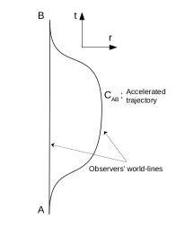
Figure 1: Schematic illustration of the trajectories (world-lines) of two observers, one at rest and the other accelerated. The accelerated trajectory correspond to the curve $C_{AB}$.

In terms of the reference frame of the observer at rest $\{\tau^{r},\bm{x}\}$, the accelerated observer’s proper time $\tau^{a}$ between the two events $A$ and $B$ reads

$$\tau^{a}_{AB}=\int_{C_{AB}}d\tau^{a}=\int_{C_{AB}}\sqrt{1-\frac{v^{2}}{c^{2}}}~{}d\tau^{r},$$ (12)

according to Eq. (9), with $\bm{v}=d\bm{x}/d\tau^{r}$, and where $C_{AB}$ is the accelerated trajectory of the accelerated observer in the reference frame of the observer at rest. Given a trajectory $C_{AB}$, one can derive the proper time of the accelerated observer elapsed between the events $A$ and $B$. It is worth noting that Eq. (12) would not maintain the same form if one attempts to derive the proper time elapsed for the rest observer from the coordinates of the accelerated observer. This is because the Minkowski metric (Eq. 9) does not remain invariant for an accelerated reference frame $\{\tau^{a},\bm{X}\}$. In the proper reference frame of an accelerated (but non-rotating) observer, the metric Eq. (9) would instead read (Ni and Zimmermann, 1978)

$$c^{2}d\tau^{2}=\left(1+\frac{\bm{a}\cdot\bm{X}}{c^{2}}\right)^{2}c^{2}(d\tau^{a})^{2}-dX^{2}-dY^{2}-dZ^{2},$$ (13)

where $\bm{a}$ is the acceleration of the proper reference frame of an accelerated observer. This fact alone dispels any paradox, as the situations of the two observers are distinct both physically and mathematically. From Eq. (12), one can infer that the elapsed proper time of an observer who has been accelerated between two arbitrary spacetime events $A$ and $B$ is always smaller than the elapsed proper time of an observer at rest $\tau^{a}_{AB}<\tau^{r}_{AB}$. In other words, this means that for an inertial observer the following action

$$S=-mc^{2}\int d\tau=-mc^{2}\int\sqrt{1-\frac{v^{2}}{c^{2}}}dt=\int L_{SR}(x^{\alpha},v^{\alpha})dt,$$ (14)

is maximal, where $L_{SR}$ is, therefore, the Lagrangian of motion of special relativity:

$$L_{SR}=-mc^{2}\sqrt{1-\frac{v^{2}}{c^{2}}}.$$ (15)

2.1.3 Free fall and proper time in general relativity

In general relativity, the free fall of a point mass $m$ aslo maximizes the proper time $\tau$, but which is now defined by

$$\tau_{AB}=\int_{C_{AB}}\sqrt{-g_{\alpha\beta}dx^{\alpha}dx^{\beta}},$$ (16)

where $C_{AB}$ means that the integration is taken along a given path between the spacetime positions $A$ and $B$ of the observer. In cartesian coordinates for instance, one has $x^{i}=(x,y,z)$. $g_{\alpha\beta}$ is the spacetime metric, which depends on the position, and which represents the curvature of spacetime. As we will see below, the metric is solution of the Einstein-Hilbert equation of general relativity.

The definition of the proper time for an observer in Eq. (16) is true whether or not the motion of the observer is accelerated. It is important to keep in mind that unlike in Newton’s theory, a free falling observer in general relativity has an inertial motion—that is, it is not accelerated. In general relativity, inertial bodies follow geodesics of spacetime that correspond to free fall trajectories. This is forced upon the theory by the equivalence principle, which states that the inertial mass is indeed equivalent to the gravitational mass.

But since the free fall of an observer maximizes its proper time, it means that Eq. (16) has to be an extremum in the case of a free fall motion. It means that the path $C_{AB}$ between the events $A$ and $B$ must be such that it extremizes Eq. (16). As a consequence, it must follow the Least Action Principle of Lagrangian mechanics that demandes the extremization of an action defined upon a Lagrangian. Indeed, from Eq. (16), one can define the following action

$$S=mc^{2}\tau=\int L(x^{\alpha},v^{\alpha})dt,$$ (17)

where $v^{\alpha}=c~{}dx^{\alpha}/dx^{0}=dx^{\alpha}/dt$ is a velocity expressed in terms of the coordinates $\{x^{\alpha}\}$ and where the Lagrangian reads

$$L=mc^{2}\sqrt{-g_{\alpha\beta}(x^{\sigma})v^{\alpha}v^{\beta}}.$$ (18)

The Least Action Principle demands that $\delta S=0$. Given a specific spacetime metric $g_{\alpha\beta}$, one can therefore compute the equations of motion by applying the Euler-Lagrange equation on Eq. (18). The equation can also be applied on the formal definition of equation Eq. (18) and one then gets the general form—that is, for all spacetime metrics—of the equations of motion (for massive point particles) that reads

$$\frac{d^{2}x^{\alpha}}{dt^{2}}=\left(\Gamma^{\alpha}_{\sigma\epsilon}-\Gamma^{0}_{\sigma\epsilon}\frac{v^{\alpha}}{c}\right)v^{\sigma}v^{\epsilon},$$ (19)

where

$$\Gamma^{\gamma}_{\alpha\beta}:=\frac{1}{2}~{}g^{\gamma\sigma}(\partial_{\alpha}g_{\sigma\beta}-\partial_{\beta}g_{\alpha\sigma}-\partial_{\sigma}g_{\alpha\beta}),$$ (20)

is named the Christoffel connection with $g^{\gamma\sigma}$, the contravariant metric—which is such that $g_{\alpha\sigma}g^{\sigma\beta}=\delta_{\alpha\beta}$, where $\delta$ is the Kronecker symbol. Besides, an accelerated trajectory would read

$$\frac{d^{2}x^{\alpha}}{dt^{2}}-\left(\Gamma^{\alpha}_{\sigma\epsilon}-\Gamma^{0}_{\sigma\epsilon}\frac{v^{\alpha}}{c}\right)v^{\sigma}v^{\epsilon}=F^{\alpha},$$ (21)

where $F^{\alpha}$ is the force responsible for the acceleration.

2.1.4 Einstein-Hilbert equation and the Newtonian approximation

The spacetime metric is curved by the energy of matter according to the Einstein-Hilbert equation that reads

$$R_{\alpha\beta}-\frac{1}{2}g_{\alpha\beta}R=\frac{8\pi G}{c^{4}}T_{\alpha\beta},$$ (22)

where $R_{\alpha\beta}$ is the Ricci tensor (see sec 2.1.5) defined as

$$R_{\alpha\beta}=\partial_{\mu}\Gamma_{\alpha\beta}^{\mu}-\partial_{\beta}\Gamma_{\alpha\mu}^{\mu}+\Gamma_{\sigma\mu}^{\mu}\Gamma_{\alpha\beta}^{\sigma}-\Gamma_{\sigma\beta}^{\mu}\Gamma_{\alpha\mu}^{\sigma},$$ (23)

and

$$R=g^{\sigma\epsilon}R_{\sigma\epsilon}$$ (24)

is the Ricci scalar, and $T_{\alpha\beta}$ is the stress-energy tensor of the material fields—which we will define in Sec. 2.1.6. The stress-energy tensor represents the energy content of the matter fields that generate the curvature of spacetime. Otherwise, we will see below that $G$ corresponds to the constant of Newton, also known as the gravitational constant.

The Newtonian approximation

In the Newtonian formalism given in Sec. 2.1.1, we assume that the speed of the considered bodies is small with respect to the speed of light $v^{2}/c^{2}\ll 1$. Let us add the constant $-mc^{2}$ to this Lagrangian, which does not impact the equation of motion, but which is such that one reproduces the Lagrangian of motion of special relativity equation Eq. (15) at leading order when $U=0$, that is

$$L_{SR}=-mc^{2}\sqrt{1-\frac{v^{2}}{c^{2}}}=-mc^{2}\left(1-\frac{v^{2}}{2c^{2}}\right)+\mathcal{O}\left(\frac{v^{4}}{c^{4}}\right).$$ (25)

Now, the Lagrangian of motion for the theory of Newton reads

$$L_{N}=-mc^{2}\left(1-\frac{v^{2}}{2c^{2}}-\frac{U}{c^{2}}\right).$$ (26)

Let us stress that for an orbit, one has $v^{2}/c^{2}\sim U/c^{2}\ll 1$ in the theory of Newton. This approximation ought to remain valid at leading order in general relativity in the weak field limit. As a consequence, for now on, we will use the notation $\mathcal{O}(c^{-2n})$ to refer to both $\mathcal{O}(v^{2n}/c^{2n})$ and $\mathcal{O}(U^{n}/c^{2n})$. Since the theory of Newton is already accurate in the solar system, we expect the theory of general relativity to reproduce the trajectories of the Newtonian theory at leading order. Therefore, one expects that there exists a spacetime metric that reproduces the Lagrangian equation Eq. (26) at leading order. One can check that injecting the following metric in Eq. (18)

$$-c^{2}d\tau^{2}=ds^{2}=-\left(1-\frac{2U}{c^{2}}\right)c^{2}dt^{2}+dx^{2}+dy^{2}+dz^{2},$$ (27)

where $ds$ is the spacetime line element defined as $ds^{2}=g_{\alpha\beta}dx^{\alpha}dx^{\beta}$, gives back the Lagrangian of motion of the theory of Newton equation Eq. (26), up to corrections of order $\mathcal{O}(c^{-4})$. Therefore, one expects the metric in Eq. (27) to be solution of general relativity at leading order for the kind of weakly gravitating sources that we have in the solar system. It can be indeed verified that by injecting the metric Eq. (27) in the Einstein-Hilbert equation Eq. (23), the resulting differential equation reads

$$\Delta U=-4\pi G\rho_{m}+\mathcal{O}(c^{-2}),$$ (28)

where $\rho_{m}$ is the mass density of the gravitational sources defined as $\rho_{m}=T^{00}/c^{2}+\mathcal{O}(c^{-2})$. It corresponds to Newton’s universal law of gravitation as long as $G$ is indeed the gravitational constant. One has therefore identified $G$ in Eq. (22) to Newton’s constant from the weak-field and slowly moving limit of the theory that leads to the same field equation as Newton’s theory at leading order.

Therefore, general relativity produces the same trajectories at leading order as Newton’s theory. This is called the Newtonian approximation of general relativity.

However, let us stress that even at this level of approximation, the two theories differ drastically—in a way that can be tested at the experimental level already. Indeed, in general relativity, the variation of an observer proper time $d\tau$ (Eq. 27) with respect to the proper time of another observer depends explicitly on their different positions in a gravitational potential $U$. This means that two observers at different locations in the gravitational potential will not agree on the evolution of time. This effect, although minute, can be tested if one has accurate enough clocks. In other words, had we developed atomic clocks with sufficient precision prior to our ability to observe the motions of celestial bodies in the solar system, we could have confirmed the superiority of general relativity over Newton’s theory. This could have been achieved by comparing the frequencies of two clocks located at different positions relative to the geoid. However, due to our atmosphere’s transparency, astronomers identified the limitations of Newton’s theory through the anomalous advance of Mercury’s perihelion—see Table 1 for the numerical value of this advance—before quantum physicists could create sufficiently accurate atomic clocks. We will further discuss the advance of the perihelion of Mercury in Sec. 2.1.8.

Finally, one can see in Eq. (27) that space it flat at leading order, such that free fall trajectories in the solar system are essentially the consequence of the curvature of the temporal dimension, not the spatial one.

Gauge invariance of Newton’s equation and the definition of coordinate times

Newton’s equation Eq. (28) is notably invariant under the following change of the potential:

$$U\rightarrow U+a_{k}(t)x^{k}+b(t),$$ (29)

where $a_{k}(t)$ and $b(t)$ are arbitrary three-vector and scalar that depend on time. One often says that the Eq. (28) is invariant under the change of gauge defined by Eq. (29).

The change of gauge in Eq. (29) corresponds to a change of the coordinate time being used to describe a motion. This is a major difference with respect to Newton’s theory where there is a unique time. A coordinate time is simply a mathematical construction of a time that can be related to the proper time of an observer, but not necessarily. For instance, it can simply be defined according to purely mathematical criteria, such as the simplicity of the field equations.

In order to illustrate the dependence of the Newtonian potential to the coordinate time being used, let us define a coordinate time that would correspond to the proper time of an imaginary observer that is so remote from the barycenter of the solar system that it can be at rest with respect to the solar system because the potential of the solar system and its gradient at their location is negligible. Assuming that this imaginary observer is indeed at rest with respect to the solar system, this means that the coordinate time $t$ corresponds to the (fictional) proper time $\tau$ such that $dt=d\tau$ at the location of this (fictional) observer. The Newtonian potential in this gauge—or, equivalently, with this coordinate time—reads

$$U(x^{i},t)=\sum_{A}\frac{Gm_{A}}{\lvert x^{i}-x^{i}_{A}(t)\rvert},$$ (30)

where $m_{A}$ and $x^{i}_{A}(t)$ are the masses and the positions of the bodies $A$. Alternatively, one could define a coordinate time that corresponds to a (fictional) observer that would be at rest at the center of the coordinate system $x^{i}=0$. In this gauge, the Newtonian potential would instead read

$$U(x^{i},t)=\sum_{A}Gm_{A}\left[\frac{1}{\lvert x^{i}-x^{i}_{A}(t)\rvert}-\frac{1}{\lvert x^{i}_{A}(t)\rvert}-\frac{x^{j}x_{A}^{j}(t)}{{\lvert x^{i}_{A}(t)\rvert}^{3}}\right],$$ (31)

because having $dt=d\tau$ in Eq. (27) at the center imposes $U(x^{i}=0)=0$, and being at rest imposes $\vec{\nabla}U\rvert_{x^{i}=0}=0$. The transformation from the potential expressed in the coordinate time of a remote observer to the potential expressed in the coordinate time of an observer at the center of the coordinate system takes the form of Eq. (29) with

$$a^{k}(t)=-\sum_{A}Gm_{A}\frac{x_{A}^{k}(t)}{{\lvert x^{i}_{A}(t)\rvert}^{3}}\qquad\textrm{, and }\qquad b(t)=-\sum_{A}\frac{Gm_{A}}{\lvert x^{i}_{A}(t)\rvert}.$$ (32)

This notably means that the leading order of the equation of general relativity is invariant under specific changes of time coordinate. As we will see in Sec. 2.1.5, this is a leftover of the invariance of general relativity through a change of coordinate system. It is really important to notice that while the field equation Eq. (28) is invariant under some changes of the coordinate time, the actual solution of the potential is not, as one can check from Eqs. (30) and (31).

In the coordinate time defined as the proper time of the fictional remote observer $t=\tau_{r}$, the proper time of fictional observer at the center of the coordinate system $\tau_{o}$ reads

$$\tau_{o}=t-\frac{1}{2c^{2}}\int\sum_{A}\frac{Gm_{A}}{\lvert x^{i}_{A}(t)\rvert}dt,$$ (33)

provided that they are indeed at rest with one another. See Sec. 3.2.2 for a discussion on the coordinate times that are used by the community, following the IAU recommendations (Soffel, 2003).

Dependence of a coordinate time to the trajectories of the gravitational bodies

Eq. (33) teaches us something very important. Depending on its definition, a coordinate time can depend explicitly on the trajectories of the gravitational bodies ${\bf x}_{A}(t)$. As a consequence, in order to define such a coordinate time in practice, it is necessary to estimate the positions of the celestial bodies over time with enough accuracy.

But why would one want to define such a coordinate time if it means that one must already have an accurate knowledge of the trajectories of the gravitational bodies in order to define it? Simply because one has to define such a coordinate time in order to compare different observations made at various locations by several observers. The proper time of each observer is indeed different and the differences between the various proper times depend on the observers’ relative trajectories in the gravitational potential. Therefore, in order to compare the various observations, one first has to define a coordinate time that will be used to transform the proper time of every observer to this coordinate time, such that after the transformation, all the observations are expressed in a common time. We will see in Sec. 2.1.7 that at the post-Newtonian level—or, the next-to-leading order—similar considerations must be taken into account for the definition of space.

Any definition of a coordinate time could be used in theory. However, in practice, a coordinate time is usually defined as being the proper time of a fictional observer at some convenient location in the solar system, such as at its barycenter or at the geoid of the Earth. Such coordinate times are defined by the International Astronomical Union, as we will further discuss in Sec. 3.2.2.

But since one needs to know the trajectories of the gravitational bodies in the solar system in order to construct this coordinate time, it means that one needs to use planetary ephemerides to construct such a time. Therefore, planetary ephemerides actually deliver the coordinate times defined by the International Astronomical Union to the community, as discussed more in details in Sec. 3.2.2.

Rotating reference frames

The Newtonian approximation of the spacetime metric in general relativity assumes the form of Eq. (27) only within a specific category of coordinate systems, typically referred to as inertial frames. Notably, the coordinate system must be kinematically non-rotating relative to distant celestial objects such as quasars. This suggests that the rotation (or absence thereof) of a local reference frame must be defined in relation to exceedingly distant objects. In support of his theory, Newton posited this coincidence as evidence of an absolute space, serving as the stage for dynamic events and providing a reference for defining rotation. In contrast, figures such as Leibniz and later Mach, contended that this apparent coincidence reveals that inertia is relative, depending more on the universe matter content than on an absolute space. Heavily influenced by these perspectives, Einstein proposed the principle of inertia relativity, later referred to as Mach’s principle (Einstein, 1918). This principle stipulates that spacetime is wholly determined by its matter content. Considering general relativity accommodates vacuum solutions, whether Einstein’s theory satisfies the principle of inertia relativity remains debated (Barbour and Pfister, 1995). However, practically speaking, the solar system asymptotic metric must be integrated into the larger spacetime metric effectively generated by distant sources. This requirement accounts for why inertial reference frames are non-rotating relative to very remote sources in general relativity—assuming they can be approximated as stationary due to their minimal angular velocity in the sky over certain timescales.

2.1.5 Invariance of the laws through a change of coordinate system

Tensors

The tensorial nature of the Einstein-Hilbert equation Eq. (22) enforces the covariance principle, which demands that the laws of Nature do not depend on the choice of the coordinate system. Indeed, tensorial equations—such as Eq. (22)—are invariant under change of coordinates. A tensor is defined by the way it transforms under a change of coordinates. A tensor $W$, with $n$ contravariant indices and $m$ covariant indices transform as

$$W^{\alpha_{1}...\alpha_{n}}_{\beta_{1}...\beta_{m}}\{x^{\sigma}\}=\left(\prod_{\alpha_{k}}\prod_{\beta_{k}}\frac{\partial x^{\alpha_{k}}}{\partial X^{\mu_{k}}}\frac{\partial X^{\nu_{k}}}{\partial x^{\beta_{k}}}\right)W^{\mu_{1}...\mu_{n}}_{\nu_{1}...\nu_{m}}\{X^{\sigma}\}.$$ (34)

Tensorial equations are manifestly invariant under coordinate change, that is:

$$A_{\alpha_{1}\alpha_{2}\ldots\alpha_{n}}^{\sigma_{1}\sigma_{2}\ldots\sigma_{p}}\{x^{\sigma}\}=B_{\alpha_{1}\alpha_{2}\ldots\alpha_{n}}^{\sigma_{1}\sigma_{2}\ldots\sigma_{p}}\{x^{\sigma}\}\Leftrightarrow A_{\beta_{1}\beta_{2}\ldots\beta_{n}}^{\omega_{1}\omega_{2}\ldots\omega_{p}}\{X^{\sigma}\}=B_{\beta_{1}\beta_{2}\ldots\beta_{n}}^{\omega_{1}\omega_{2}\ldots\omega_{p}}\{X^{\sigma}\}.$$ (35)

Because the metric field is a tensor, one can notably verify with Eq. (34) that the line-element

$$ds^{2}=-c^{2}d\tau^{2}=g_{\alpha\beta}\{x^{\sigma}\}dx^{\alpha}dx^{\beta}=g_{\alpha\beta}\{X^{\sigma}\}dX^{\alpha}dX^{\beta}$$ (36)

is invariant under coordinate change. Indeed, the proper time of an observer cannot depend on any coordinate system as it is a measured quantity. Let us note however, that according to this definition, the Christoffel connection defined in Eq. (20) is not a tensor as it transforms as follow:

$$\Gamma_{\mu\nu}^{\alpha}\{x^{\sigma}\}=\frac{\partial x^{\alpha}}{\partial X^{\beta}}\frac{\partial X^{\sigma}}{\partial x^{\mu}}\frac{\partial X^{\rho}}{\partial x^{\nu}}\Gamma_{\sigma\rho}^{\beta}\{X^{\sigma}\}-\frac{\partial^{2}x^{\alpha}}{\partial X^{\sigma}\partial X^{\rho}}\frac{\partial X^{\sigma}}{\partial x^{\mu}}\frac{\partial X^{\rho}}{\partial x^{\nu}}.$$ (37)

One can also check that the difference between two connections is a tensor. What the covariance principle means in particular is that the laws of physics are independent with respect to the observer, whether the observer is inertial or not. While this is very satisfying at the fundamental level, it also implies an intrinsic ambiguity about the coordinates that one can use, as they are all equivalent in principle.

Observables

Certain coordinate systems can result in what are known as spurious effects. These are essentially false effects arising solely from the coordinate system and do not reflect reality. Determining whether an effect is genuine or spurious can be challenging unless all calculations are made with respect to actual observables. Parameters referred to as observables are independent of the coordinate system, and therefore, can correspond to quantities that an observer can directly measure. These include values such as the proper time elapsed for an observer between two events, or, as we will discuss shortly, the angle between two light cones at the observer’s location. On the contrary, it is very important to keep in mind that positions, trajectories, or velocities, are not observables, but have to be reconstructed from observations after assuming a specific coordinate system—as well, as we will see, as a model for the dynamics of bodies and light.

Observables Are Scalar Quantitites

According to Eq. (34), the only type of tensors that do not depend on the coordinate system are scalars, which are such that

$$S\{x^{\sigma}\}=S\{X^{\sigma}\}.$$ (38)

Tensors, if not scalars, therefore cannot represent observable quantities.

Positions in two dimensions: Projection on the Celestial Sphere

From an observer’s perspective, the only tangible element related to the spatial distribution of any distant object is the relative angular separation in the sky between the images of two objects. This measurement can be made without reference to any specific coordinate system. This angular separation corresponds to angles between the light cones connecting the distant objects to the observer at the observer’s location, as shown in Figure 2.

However, observers typically project at their location the vector of the light cones, which join the distant objects to the observer’s location, onto a coordinate-dependent representation of their celestial spheres. This process is where coordinate systems become to be used. Importantly, it must be noted that the relative position (angle) of the same distant objects as viewed by two different observers can vary. This is because in general relativity, both time and space are relative to the observer and to its gravitational environment. Hence, there is no such thing as absolute positions. In simpler terms, the celestial spheres for different observers differ in general. Although this effect is minute for observers in the solar system, it nonetheless needs to be accounted for in modern astrometry.

In practical terms, an object location on the celestial sphere is determined by observing the angular separation in the sky between the object and reference points like quasars, from the perspective of the observer. Indeed, due to their extremely remote location, the apparent movement of these reference points is negligible at the present level of accuracy for the astrometric measurements for these objects (see Sec. 3.2.3), and they can therefore indeed serve as static reference points (or astrometric candle light).

However, there is another significant effect to consider, which is also illustrated in Fig. 2: the propagation of light is not generally linear. This means that if an observer sees a remote object at a particular location on his celestial sphere, it doesn’t imply that the object is actually at that position on the sphere. This effect is referred to as gravitational lensing (or deflection of light in the solar system) and is due to the fact that light propagates on null-geodesics, see Sec. 2.1.9—which are not straight lines in general. Although its impact is relatively weak for objects within the solar system, it highlights the inherent difficulty of attributing positions on the celestial sphere in general relativity.

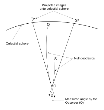
Figure 2: Schematic illustration of the angle ($\alpha$) determined by an observer (O) at their location, between two null-geodesics—see Sec. 2.1.9—that link the observer to two sources (Q and S) of electromagnetic waves. Each null-geodesic represents a segment of the light-cone centered on an emitter.

Hence, assigning a two-dimensional position to an object in general relativity not only necessitates the definition of a coordinate system, but also requires a model of the gravitational field through which light has propagated. Consequently, any position in general relativity is model-dependent and is essentially a reconstruction from observations.

The Third Dimension: Range

There are various methods to infer the distance between a remote object and an observer. For s/c, the most accurate technique is typically the measure of the time delay between the emission of a signal in the direction of the spacecraft and the reception of the returned signal by the probe (ranging). Essentially, this involves measuring the round-trip time of an electromagnetic signal emitted at a given frequency between an observer and a spacecraft. Given that the signal propagates at a constant speed in vacuum, this propagation time can be converted into a distance. However, while the signal indeed travels at the speed of light in a vacuum locally, its propagation time measured by a given observer can be affected by the gravitational field localised between the source of emission and this observer, along the trajectory of the electromagnetic signal. As a result, even when a the signal follows a straight line between two points, the propagation time would not correspond to the Euclidean distance between these points divided by the speed of light. This effect is known as the Shapiro delay—See Sec. 2.1.9.

Therefore, determining distances through ranging techniques not only depends on the specific choice of the coordinate system considered but also depends on the knowledge one has on the gravitational potential in the solar system. Consequently, distances are both model and theory dependent. Indeed, the potential in the solar system is reconstructed by solving the field equations of a given theory—e.g. Eq. (27)—after assuming a specific model for the solar system that “sources” the field equations—e.g. the right hand side of Eq. (27).

Let us stress in particular that a modification of the field equations of general relativity therefore implies the need for a new analysis of the measures, leading to a new determination of the distances.

The Need of Conventions for Coordinate Systems

Because space and time are relative, for various observers to compare their respective observations and agree on the positions of bodies, they must define a set of coordinates that allows to convert their respective observations in terms of positions in space and time. This is the role of the IAU recommendations that we will discuss in Sec. 3.2.

2.1.6 The action of general relativity

Just as the equations of motion can be derived from the Euler-Lagrange equation, the field equation of general relativity can be derived from a Lagrangian density that is defined based on the metric field and the various material fields. The key difference lies in the type of dynamical variables used in the Lagrangian: instead of using position and velocity as dynamical variables, one considers the fields and their derivatives as dynamical variables in the case of a Lagrangian density. One can define the action of general relativity as follows

$$S_{GR}=\int\sqrt{-g}d^{4}x\left[\frac{R}{2\kappa}+\mathcal{L}_{m}\right],$$ (39)

where $g$ is the metric determinant, $\mathcal{L}_{m}$ the Lagrangian density of matter fields, and $\kappa=8\pi G/c^{4}$ the coupling constant between matter and curvature. In order to derive the Euler-Lagragian equation, $R$ is treated as a functional constructed upon the metric field and its derivative—see Eq. (24). $\mathcal{L}_{m}$ is then a functional constructed upon the matter fields and their derivative. For instance, for an electromagnetic field one has

$$\mathcal{L}_{m}=\frac{1}{4\mu_{0}}g^{\alpha\sigma}g^{\beta\epsilon}(\partial_{\alpha}A_{\beta}-\partial_{\beta}A_{\alpha})(\partial_{\sigma}A_{\epsilon}-\partial_{\epsilon}A_{\sigma})$$ (40)

where $\mu_{0}$ is the magnetic permeability of vacuum, and $A^{\alpha}$ is the electromagnetic four-vector. Let us note that one has $A^{\alpha}=(\phi/c,\bm{A})$ where $\phi$ is the scalar potential and $\bm{A}$ the vector potential of classical electromagnetism, form which one can compute the electric and magnetic fields (Jackson, 1998).

Defining a theory from its action rather than from its equations is convenient because it allows one to be sure that the theory possesses conservation laws for the considered theory, which derive from Noether’s theorem that states that every symmetry of a Lagrangian implies the existence of a conservation law (Noether, 1918; Wald, 1984). Therefore, most modern theories are defined from an action, although there are some exceptions—such as MOND, see Sec. 4.7.

Applying the principle of least action on the action (39), one recovers the Einstein-Hilbert equation of general relativity Eq. (22), with

$$T_{\alpha\beta}=-\frac{2}{\sqrt{-g}}\frac{\delta(\sqrt{-g}\mathcal{L}_{m})}{\delta g^{\alpha\beta}},$$ (41)

where $\delta$ stands for a variational derivative. It is worth noting that from Noether’s theorem, the diffeomorphism invariance—that is, the invariance under change of coordinates—of the matter Lagrangian $\mathcal{L}_{m}$ implies the (covariant) conservation of the stress-energy tensor

$$\nabla_{\sigma}T^{\mu\sigma}=0,$$ (42)

where $\nabla_{\sigma}$ is the covariant derivative defined as followed for a tensor $X$ with $k$ contravariant indices and $l$ covariant indices:

$$\nabla_{\sigma}X^{\mu_{1}...\mu_{k}}_{\nu_{1}...\nu_{l}} = \partial_{\sigma}X^{\mu_{1}...\mu_{k}}_{\nu_{1}...\nu_{l}}$$

$$+\Gamma^{\mu_{1}}_{\sigma\lambda}X^{\lambda...\mu_{k}}_{\nu_{1}...\nu_{l}}+...+\Gamma^{\mu_{k}}_{\sigma\lambda}X^{\mu_{1}...\lambda}_{\nu_{1}...\nu_{l}}$$

$$-\Gamma^{\lambda}_{\sigma\nu_{1}}X^{\mu_{1}...\mu_{k}}_{\lambda...\nu_{l}}-...-\Gamma^{\lambda}_{\sigma\nu_{l}}X^{\mu_{1}...\mu_{k}}_{\nu_{1}...\lambda}.$$

This is, of course, consistent with the geometrical fact that $\nabla_{\sigma}G^{\mu\sigma}=0$, with $G^{\mu\nu}=R^{\mu\nu}-1/2~{}g^{\mu\nu}R$, the Einstein tensor, where $R^{\mu\nu}$ is the contravariant Ricci tensor defined from the covariant Ricci tensor $R_{\mu\nu}$ and the contravariant metric tensor $g^{\mu\nu}$ as $R^{\mu\nu}=g^{\mu\alpha}g^{\nu\beta}R_{\alpha\beta}$.

2.1.7 The post-Newtonian approximation of general relativity and gauge invariance

First, let us recall that the metric of general relativity at the Newtonian level, for a reference frame that is not kinematically rotating with respect to distant celestial bodies, reads

$$g_{00}=-1+\frac{2U}{c^{2}}+\mathcal{O}(c^{-3}),$$ (44)

$$g_{0i}=\mathcal{O}(c^{-2}),$$ (45)

$$g_{ij}=\delta_{ij}+\mathcal{O}(c^{-1}),$$ (46)

such that one indeed has

$$ds^{2}=-\left(1-\frac{2U}{c^{2}}\right)c^{2}dt^{2}+dx^{2}+dy^{2}+dz^{2},$$ (47)

at leading order. The truncation between leading and next-to-leading orders in Eqs. (44-46) are made with respect to the equation of motion that derives from the Lagrangian of motion Eq. (18). Indeed, the Lagrangian of motion with Eqs. (44-46) reads

$$L\propto 1+\frac{1}{c^{2}}\left(\frac{v^{2}}{2}-U\right)+\mathcal{O}(c^{-3}).$$ (48)

One can show that a set of coordinate systems exists in general relativity that are such that, at next-to-leading order, the metric reads (Damour et al., 1991)

$$g_{00}=-1+\frac{2w}{c^{2}}-\frac{2w^{2}}{c^{4}}+\mathcal{O}(c^{-5}),$$ (49)

$$g_{0i}=-\frac{4w^{i}}{c^{3}}\mathcal{O}(c^{-4}),$$ (50)

$$g_{ij}=\delta_{ij}\left(1+\frac{2w}{c^{2}}\right)+\mathcal{O}(c^{-3}),$$ (51)

where $w$ and $w^{i}$ are gravitational potentials. This is the so-called post-Newtonian metric of general relativity, in conformally cartesian coordinates. Assuming this metric, the field equation of general relativity reduces to

$$\Delta w+\frac{3}{c^{2}}\partial_{tt}^{2}w+\frac{4}{c^{2}}\partial_{tj}^{2}w_{j}=-4\pi G\sigma+O\left(c^{-3}\right),$$ (52)

$$\Delta w_{i}-\partial_{ij}^{2}w_{j}-\partial_{ti}^{2}w=-4\pi G\sigma^{i}+O\left(c^{-2}\right),$$ (53)

where $\sigma=c^{-2}(T^{00}+T^{kk})$ and $\sigma^{i}=c^{-1}T^{0i}$, such that $\sigma$ and $\sigma^{i}$ are zeroth order quantities—because $T^{\mu\nu}=\mathcal{O}(c^{2},c,c^{0})$ in the weak-field and slowly moving approximation.

Post-Newtonian gauge invariance

One can check that the equations Eqs. (52-53) are invariant under the following transformations

$$w^{\prime}=w-\frac{1}{c^{2}}\partial_{t}\lambda,$$ (54)

$$w_{i}^{\prime}=w_{i}+\frac{1}{4}\partial_{i}\lambda,$$ (55)

where $\lambda$ is an arbitrary differential function. Indeed, while the form of the metric in Eqs. (49-51) completely fixes the type of spatial coordinates being considered, it leaves a freedom at the level of the time coordinate. This gauge invariance indeed corresponds to a shift of the time variable

$$\delta t=c^{-4}\lambda(x^{\alpha}).$$ (56)

After having imposed a non-kinematically-rotating frame with respect to distant celestial objects (such as quasars), a central world-line and the use of conformally cartesian coordinates, Eq. (56) is a remaining freedom of our coordinate system.

Harmonic gauge

The International Astronomical Union recommends (Soffel, 2003) the use of harmonic coordinates that are such that

$$g^{\alpha\beta}\Gamma^{\sigma}_{\alpha\beta}=\mathcal{O}(c^{-5},c^{-4}).$$ (57)

However, because of the use of conformally cartesian coordinates, the space component of this condition $g^{\alpha\beta}\Gamma^{i}_{\alpha\beta}=\mathcal{O}(c^{-4})$ is already satisfied, and one is left with the time component of this condition that, considering the metric Eqs. (49-51), reduces to

$$\partial_{t}w+\partial_{j}w_{j}=\mathcal{O}(c^{-2}).$$ (58)

With this condition, Eqs. (52-53) reduce to

$$\square_{m}w=-4\pi G\sigma+O\left(c^{-3}\right),$$ (59)

$$\triangle w_{i}=-4\pi G\sigma^{i}+O\left(c^{-2}\right),$$ (60)

where $\square_{m}$ and $\triangle w_{i}$ are respectively the d’Alembertian and Laplacian of the usual flat Minkowski spacetime:

$$\square_{m}=-c^{-2}\partial^{2}_{tt}+\triangle,$$ (61)

where, for instance, $\triangle=\partial^{2}_{xx}+\partial^{2}_{yy}+\partial^{2}_{zz}$ in Cartesian coordinates.

2.1.8 The Einstein-Infeld-Hoffman-Droste-Lorentz equation of motion

Up to corrections that can be taken into account at a later stage, celestial bodies in the solar system can be approximated as being non-rotating point particles. This approximation has been explored for the first time by Lorentz and Droste (Lorentz and Droste, 1917a, b)—translated in (Lorentz and Droste, 1937)—and re-derived later by Einstein, Infeld and Hoffman (Einstein et al., 1938). The stress-energy tensor for point particles is simply the stress-energy tensor of a dust fluid

$$T^{\mu\nu}=\rho_{m}u^{\mu}u^{\nu},$$ (62)

where $u^{\alpha}=dx^{\alpha}/d\tau$ is the proper four-velocity of the fluid. In terms of conserved mass along the fluid geodesics $dm_{A}/d\tau=0$, it reads

$$T^{\mu\nu}=\sum_{A}\frac{m_{A}~{}u^{0}/c}{\sqrt{-g}}v_{A}^{\mu}v_{A}^{\nu}\delta^{(3)}(\bm{x}-\bm{x}_{A}(t)),$$ (63)

where $\delta^{(3)}$ is the 3-dimensional delta function, and $v^{\alpha}=dx^{\alpha}/dt$ the coordinate four-velocity of the fluid, such that $u^{\alpha}=u^{0}v^{\alpha}/c$. Eq. (63) used the fact that $u_{\mu}\nabla_{\sigma}T^{\mu\sigma}=0$ —which follows from Eq. (42)—such that one has the usual Newtonian conservation of the mass density $\partial_{\sigma}(\rho^{*}v^{\sigma})=\partial_{t}\rho^{*}+\partial_{i}(\rho^{*}v^{i})=0$ for the density $\rho^{*}:=\sqrt{-g}\rho_{m}u^{0}/c$. Solving the Einstein-Hilbert equation Eq. (22) with this approximation, and in the harmonic gauge Eq. (58), leads to the metric in Eqs. (49-51) with

$$w=w_{0}-\frac{1}{c^{2}}\Delta+O(c^{-4}),$$ (64)

$$w^{i}=\sum_{A}\frac{Gm_{A}}{r_{A}}v_{A}^{i}+O(c^{-2}),$$ (65)

where

$$w_{0}=\sum_{A}\frac{Gm_{A}}{r_{A}},$$ (66)

where $\bm{r}_{A}=\bm{x}-\bm{x}_{A}(t)$, $r_{A}=\lvert\bm{r}_{A}\rvert$, and

$$\Delta=\sum_{A}\frac{Gm_{A}}{r_{A}}\left\{-2v_{a}^{2}+\sum_{B\neq A}\frac{Gm_{B}}{r_{BA}}+\frac{1}{2}\left[\frac{\left({\bm{r}_{A}}\bm{v_{A}}\right)^{2}}{r_{A}^{2}}+{\bm{r}_{A}}{\bm{a}_{A}}\right]\right\},$$ (67)

with $r_{AB}=\lvert\bm{x}_{B}-\bm{x}_{A}\rvert$. We should note that this corresponds to the metric recommended by the International Astronomical Union (Soffel, 2003), subject to corrections accounting for the fact that celestial bodies are not point-like but extended objects, and that these bodies possess angular momentum relative to the frame that is fixed with respect to distant objects, such as quasars. Fortunately, these corrections are numerically small, such that they can safely be added a posteriori at the leading order, without impacting the calculation of the next-to-leading order.

Now, injecting this metric into the definition of the Lagrangian of motion Eq. (18), one gets for a test particle $B$ the following Lagrangian of motion

$$L_{B} =-m_{B}c^{2}+m_{B}\frac{v_{B}^{2}}{2}+\sum_{A\neq B}\frac{Gm_{A}m_{B}}{r_{AB}}+\frac{m_{B}v_{B}^{4}}{8c^{2}}$$

$$+\frac{1}{c^{2}}\sum_{A\neq B}\frac{Gm_{A}m_{B}}{r_{AB}}\left[-4\bm{v}_{A}\cdot\bm{v}_{B}+\frac{3}{2}v_{B}^{2}+2v_{A}^{2}-\frac{(\bm{v}_{A}\cdot\bm{r}_{AB})^{2}}{2r_{AB}^{2}}-\frac{\bm{r}_{AB}\cdot\bm{a}_{A}}{2}\right]$$

$$-\frac{1}{c^{2}}\sum_{A\neq B}\frac{Gm_{A}m_{B}}{r_{AB}}\left[\sum_{D\neq A}\frac{Gm_{D}}{r_{AD}}+\sum_{D\neq B}\frac{1}{2}\frac{Gm_{D}}{r_{DB}}\right]+\mathcal{O}(c^{-4}).$$

Injecting this Lagrangian into the Euler-Lagrange equation Eq. (7), one finally gets the Einstein-Infeld-Hoffman-Droste-Lorentz (EIHDL) equation of motion given in Eq. (90) in Sec. 3.3.

The advance of perihelion of Mercury

When focusing solely on the two-body problem, one can examine the secular changes of the orbital elements by treating the $c^{-4}$ term in the equation of motion Eq. (90) as perturbations to Keplerian orbits. For instance, the secular advance of a perihelion in the two-body problem can be expressed as follows

$$\Delta\dot{\varpi}=6\pi\frac{G(m_{1}+m_{2})}{a(1-e^{2})c^{2}},$$ (68)

where $a$ is the Keplerian semi-major axis, $e$ the eccentricity and $m_{i}$ the mass of the body $i$.

2.1.9 The propagation of light in general relativity

From the Lagrangian of a free electromagnetic field Eq. (40), one derives the following equation for the free electromagnetic field in a curved spacetime

$$\nabla_{\sigma}F^{\alpha\sigma}=\partial_{\sigma}F^{\alpha\sigma}+\Gamma^{\alpha}_{\sigma\epsilon}F^{\epsilon\sigma}+\Gamma^{\sigma}_{\sigma\epsilon}F^{\alpha\epsilon}=0,$$ (69)

where $\nabla_{\sigma}$ defines the covariant derivatives associated to the Christoffel connection Eq. (2.1.6). Using the definition of the electromagnetic tensor in Sec. 2.1.6, and translating the 4-vector potential in terms of electric and magnetic fields (Jackson, 1998), one recovers the equations of Maxwell for free electromagnetic fields if spacetime is flat—that is $\Box_{m}\vec{E}=0$ and $\Box_{m}\vec{B}=0$, where $\Box_{m}$ is the usual D’Alembertian of flat Minkowski spacetimes defined in Eq. (61). Considering the Lorenz gauge $\nabla_{\sigma}A^{\sigma}=0$, Eq. (69) reduces to

$$\Box A^{\alpha}-g^{\alpha\sigma}R_{\sigma\epsilon}A^{\epsilon}=0.,$$ (70)

where one defines the covariant D’Alembertian as $\Box=g^{\sigma\epsilon}\nabla_{\sigma}\nabla_{\epsilon}$. Now, let us expand the 4-vector potential as follows (Misner et al., 1973)

$$A^{\mu}=\mathfrak{R}\left\{\left(a^{\mu}+\epsilon b^{\mu}+O\left(\epsilon^{2}\right)\right)\exp^{i\theta/\epsilon}\right\},$$ (71)

where $\mathfrak{R}\{X\}$ means the real part of $X$. The leading order in the $\epsilon$ expansion corresponds to the geometric optics approximation. It induces that

$$k^{\sigma}\nabla_{\sigma}k^{\alpha}=0,$$ (72)

where the wave-vector is defined as $k^{\alpha}:=g^{\alpha\sigma}\partial_{\sigma}\theta$ and

$$k_{\sigma}k^{\sigma}=g_{\sigma\epsilon}k^{\sigma}k^{\epsilon}=0.$$ (73)

Eq. (72) means that in the geometric optics limit, electromagnetic waves follow spacetime geodesics

$$\frac{dk^{\alpha}}{d\lambda}+\Gamma_{\mu\nu}^{\alpha}k^{\mu}k^{\nu}=0,$$ (74)

where $\lambda$ is an affine parameter of the geodesics, such that $k^{\alpha}=dx^{\alpha}/d\lambda$. Eq. (73) means that those geodesics are such that the line element is null ($ds^{2}=0$) along the trajectories of the electromagnetic waves in the geometric optics approximation. One therefore generically says that light follows null-geodesics, although this is in fact correct only in the geometric optics approximation. The fact that $ds^{2}=0$ along the geodesics of light implies that the trajectory lies on the null spacetime cones, which define the causal structure of spacetime. In other words, the speed of light is indeed equivalent to the speed $c$ appearing in the definition of the line element Eq. (36). But it also means that there is no notion of proper time for light since the line element $ds^{2}=-c^{2}d\tau^{2}$ is null along their geodesics.

Null-geodesics and astrometric observables

Because electromagnetic waves follow null-geodesics of a curved spacetime in the geometric optic approximation, the trajectories of electromagnetic waves are curved in general, notably leading to the deflection mentioned in Sec. 2.1.5 and represented in Fig. 2.

One side of astrometry is about determining the projection of the positions of celestial bodies on the celestial sphere as they are seen by an observer, based on their angular measurements. Indeed, as detailed in Sec. 2.1.5, what measures an observer are the angles between the null-cones that link them to the sources of the observed electromagnetic waves.

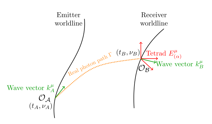
Figure 3: Illustration of an electromagnetic wave with frequency $\nu_{A}$ emitted by $\mathcal{O}_{\mathcal{A}}$ with a wave four-vector of components $k^{\mu}_{A}$ and received by $\mathcal{O}_{\mathcal{B}}$ at a frequency $\nu_{B}$ and with a wave four-vector of components $k^{\mu}_{A}$. Figure taken from (Hees et al., 2014a), with the authorization of the lead author.

As explained notably in (Hees et al., 2014a), one way to get a covariant definition of the position of the electromagnetic sources in the celestial sphere as it appears for an observer, is to use the tetrad formalism (Misner et al., 1973; Klioner and Kopeikin, 1992), by giving the direction of observation of an incoming electromagnetic wave in a tetrad $E$ comoving with the observer $\mathcal{O}_{\mathcal{B}}$, as one can see in Fig. 3. We write $E^{\mu}_{\langle\alpha\rangle}$ the components of this tetrad, where $\langle\alpha\rangle$ corresponds to the tetrad index and $\mu$ is a normal tensor index that can be lowered and raised by use of the metric. The tetrad is assumed to be orthonormal so that

$$g_{\mu\nu}E_{\langle\alpha\rangle}^{\mu}E_{\langle\beta\rangle}^{\nu}=\eta_{\langle\alpha\rangle\langle\beta\rangle},$$ (75)

$\eta$ being the flat Minkowski metric, and the vector $E^{\mu}_{\langle 0\rangle}$ is chosen to be timelike, such that $E^{\mu}_{\langle i\rangle}$ is spacelike. Then, the wave-vector $k_{\mu}=g_{\mu\nu}k^{\nu}$ becomes in the tetrad frame associated to the observer

$$k_{\langle\alpha\rangle}=E_{\langle\alpha\rangle}^{\mu}k_{\mu}.$$ (76)

The incident direction of the wave in the tetrad frame is given by the following normalization

$$n^{\langle i\rangle}=\frac{k^{\langle i\rangle}}{\sqrt{\delta_{jk}k^{\langle j\rangle}k^{\langle k\rangle}}}=\frac{k^{\langle i\rangle}}{k^{\langle 0\rangle}}=-\frac{k_{\langle i\rangle}}{k_{\langle 0\rangle}}.$$ (77)

This quantity is the actual astrometric observable at the location of the observer. For more details, we refer the reader to (Misner et al., 1973; Klioner and Kopeikin, 1992; Hees et al., 2014a).

The other side of astrometry is about determining the distance of remote objects, which leads us to the concept of the Shapiro delay.

Shapiro delay

In the solar system, most of the time, the trajectory of light can be approximated as being straight lines at leading order. That is, one has $x^{i}(t)=n^{i}c(t-t_{e})+x^{i}_{e}+\mathcal{O}(c^{-2})$—where $e$ stands for the emission, and $n^{i}$ is a constant normalized vector. One can use this information in order to compute the coordinate time elapsed between the emission and the reception of light, without the need to actually solve the geodesic equation Eq. (74). From the null condition Eq. (73), one has, indeed, that $ds^{2}=0$ between the emission and the reception of the electromagnetic wave. This means that $g_{\mu\nu}dx^{\nu}dx^{\mu}=0$, where $g_{\mu\nu}$ is given by Eqs. (49-51). However, since light travels at the speed of light, $v^{i}/c$ is not a negligible quantity, and it is necessary to maintain the same order of development in terms of $c^{-n}$ in the metric to account for all the relevant terms at a given order for the propagation of light. As a result, when considering deviations from the trajectory of light relative to special relativity up to the order $\mathcal{O}(c^{-3})$, the relevant metric is

$$ds^{2}=-\left(1-\frac{2U}{c^{2}}\right)c^{2}dt^{2}+\left(1+\frac{2U}{c^{2}}\right)(dx^{2}+dy^{2}+dz^{2})+\mathcal{O}(c^{-3})=0,$$ (78)

where $U=w+\mathcal{O}(c^{-2})$—see Eqs. (28) and (52). Integrating over this equation, one gets the coordinate time elapsed between the emission and the reception $T_{er}=t_{r}-t_{e}$

$$c~{}T_{er}=\lvert x^{i}_{r}-x^{i}_{e}\rvert+\frac{2}{c^{2}}\int_{e}^{r}Udl+\mathcal{O}(c^{-3}),$$ (79)

where the integration is taken along the straight line $x^{i}(t)=n^{i}(t-t_{e})+x^{i}_{e}$ that connects the emission and the reception events. It appears as if light experiences a delay due to the presence of a gravitational field. This delay is known as the Shapiro delay, named after Irwin Shapiro who was the first to predict this effect (Shapiro, 1964). More on this delay in Sec. 3.4.1.

Hence, the Shapiro delay has to be taken into account in order to recover the distance—in terms of a given coordinate system—from the measured round-trip propagation time. This means that distances constructed from observations not only depend on the coordinate system being used, but also depend on the model for the gravitational potential $U$ along the trajectory of the electromagnetic wave.

It is crucial to have in mind that what is typically probed by solar system experiments—such as in (Bertotti et al., 2003b)—is not so much the delay in Eq. (79), but rather its variation as the observed electromagnetic signal traverses different sections of the gravitational potential $U$. More specifically, these experiments usually probe the delay variation with respect to the the minimum distance between the electromagnetic signal trajectory and the gravitating body (also called impact parameter). For a comprehensive discussion on this topic, we direct readers to Chapter 6.3 in Wald (1984).

2.1.10 Alternative gravitational theories

All the aspects of the aforementioned content may be subject to modifications in an alternative theory to general relativity—see Sec. 4. Hence, one must exercise caution when considering alternative theories of gravity, as the introduced modifications can impact the entire modeling process—from the definition of the coordinate system, to the equations of motion of light and massive bodies—and consequently the analysis of the observations.

2.2 Basics on Ephemeris

An ephemeris is a table of positions and velocities given at different time steps. One can compute an ephemeris for artificial satellites, planetary bodies (planets, natural satellites, asteroids, comets…) but also pulsars. In order to provide to the user accurate estimations of the dynamical states of the considered body, several ingredients are necessary.

First, one needs to agree upon a set of both time and space coordinates given in a properly defined frame. This frame will be preferably inertial and the coordinate system will give an easily understandable representation of the body motion. This coordinate system will also be used to confront the dynamical modeling of the motion to the observations (see in step 3). The selection of the frame—in which the motion and the observations will be described—and its characterisation in space and time (metrics) will constitute the step 1 of the ephemeris construction (red boxes in Fig. 4).

Second, we shall identify and develop the appropriate dynamical model for describing the most accurately the motion of the bodies. This step (black box in Fig. 4) requires the writing of an equation of motion according to the frame defined in the step 1. In the dynamical modeling, one must include all the gravitational perturbations expected for the considered system. A numerical integration of the equations of motion is also usually performed in order to provide to the users positions and velocities for discrete times. Analytical resolutions were also proposed up to the beginning of the XXI century but stopped when the planetary observations became too accurate in regards to the size of the analytical series (see for example Fienga and Simon (2005)).

At this step, one may consider that the ephemeris is built. However, in particular in the solar system, the localisation of the object of interest has been monitored by observers and a comparison between its modeled and observed dynamical states (positions and velocities) is used for improving the model and then, to continue the process of construction of the ephemeris.

It is important to stress that the transformation from computed positions and velocities to observed quantities (direct radar range to the planetary surface, s/c navigation range and frequency shift, angular positions, pulsar time of arrival) requires some hypothesis on the space and time coordinate system in play and on how the observations have been obtained (see for example the Shapiro delay in Sec. 4.2.5 or Sec. 3.5). The data used for building planetary ephemerides are then not independent from the framework used for describing gravity.

In a third step, we consider the information on the positions and/or velocities obtained by the observers. As explained previously, and as it will be described in details in Sec. 3.4 in the case of planetary ephemerides, these informations are deduced from observations that can be ranges, frequency shifts, angular positions relative to reference stellar or quasi-stellar objects (part of astrometric catalogues or not) in different wavelengths (from optical to radio), in most of the cases centered on Earth or on specific locations at its surface. In general, at this step (blue boxes in Fig. 4), the observations are closely analysed in order to remove outliers, and to identify and correct potential biases and systematics.

The forth step (orange box in Fig. 4) is the confrontation between the observed quantities analysed at step 3 and the same quantities estimated with the dynamical model at step 2. From this comparison, are obtained the residuals, which are the differences between model and observations. In order to have the most accurate modelisation of the observed positions, one looks for minimizing the residuals by considering different causes:

• a mismodeling in the motion of the body. In this case, the step 2 has to be reconsidered and the dynamical modeling modified for example by adding more perturbations.

• parameters used in the model that are not close enough from their real values. The model is then corrected by updating the values of the parameters.

• some systematics or bias in the observations were not accounted for properly and still remain in the residuals. A modification of step 4 is then necessary.

It is of course not easy to isolate the different causes of the residuals. But, nevertheless, in order to reduce the differences obtained at step 4, one systematically starts with correcting the parameters of the model by using either a classic least squares method or a Bayesian approach (see for example the discussion in Sec. 3.5). Once the model has its parameters updated considering the current set of observations, if residuals still present some signatures different from white noise, one can investigate the correctness of the dynamical modeling or the data analysis procedure. This very generic procedure—-that can be used for a wide set of natural or artificial bodies—- can be sketched by Fig. 4. This Figure shows that the definition of the frame in which will be described both the motion and the observations is a crucial step for the prediction of the dynamical status of whatever object, from artificial satellites to quasi-stellar objects.

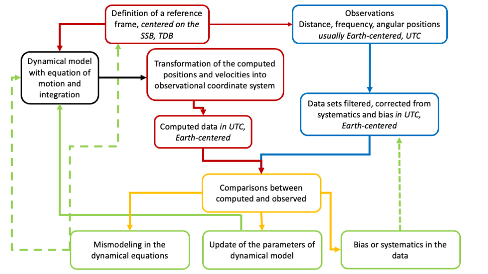
Figure 4: Schematic representation of the construction of ephemeris applied to the planetary case. SSB stands for solar system barycenter (see Sec. 3.2.4), TDB (UTC) stands for Barycentric Dynamimcal Time (Universal Time Coordinate, respectively) (see Sec. 3.2.2). The description of the dynamical model is the case of planetary ephemerides is done in Sec. 3.3, and the presentation of the observational data sets in Sec. 3.4

With the improvement of the measurement accuracy on planetary positions and velocities, the Newtonian paradigm of an universe with flat Cartesian coordinate systems and straight photon path failed to explain the observations. As discussed in introduction, the first evidence of the Newtonian failure was the case of the advance of perihelia of Mercury, explained by Einstein (1915). On Table 1, are compared the accuracies reached by three generations of planetary ephemerides and the advance of perihelia as predicted by general relativity. It is immediately visible that even with the Gaillot ephemerides in the late XIX century (Gaillot, 1888; Gaillot and Le Verrier, 1913), after three years of observations, the accumulated advance of perihelia for Mercury (1.29 seconds of arc) is greater than the observational accuracy of this epoch (1 second of arc). This leads to the choice of general relativity as a preferred framework over Newton’s laws.

However, other frameworks can also be proposed for describing the most accurate astrometric observations of planets in our solar system. In most cases, these alternative theories tend asymptotically to general relativity in the context of our weak field solar system. In Section 4, we review the alternative gravity models for which dedicated planetary ephemerides have been constructed and published in existing literature. We prioritize these models because we believe that only a fully developed ephemeris, as described in Fig. 4, can conclusively constrain, or even rule out, an alternative theory of gravitation. For a detailed discussion with examples, we refer to Section 5.

Table 1: 4 generations of planetary ephemerides: accuracies of the observations used for the construction of the ephemerides either with angular measurements (Columns labeled angle) or with direct distance radar and spacecraft tracking observations (Columns labeled distance Earth-). These values give an idea of the expected precision obtained by the ephemerides during the period of observations indicated in the second row of the Table. It does not preclude from a degradation of the quality of the ephemerides out from the period. The last column gives the estimation of the advance of perihelia $\Delta\dot{\varpi}$ as computed with general relativity. For the earth, $\Delta\dot{\varpi}$ is of about 0.1 ”.yr^-1.

Ephemerides	Gaillot		DE102		DE440/INPOP19a		GR
	Gaillot and Le Verrier (1913)		Standish (1983)		Park et al. (2021)
					Fienga et al. (2019a)
Data span	1800-1913		1913-1983		1924-2021
	angle	distance	angle	distance	angle	distance	$\Delta\dot{\varpi}$
		Earth-		Earth-		Earth-
	”	km	”	km	”	km	”.yr-1
Mercury	1	450	0.050	5	0.002	0.004	0.43
Venus	0.5	100	0.050	2	0.002	0.006	0.14
Mars	0.5	150	0.050	0.050	0.001	0.0015	0.065
Jupiter	0.5	1400	0.1	10	0.010	0.020	0.019
Saturn	0.5	3000	0.1	600	0.001	0.020	0.010
Uranus	1	12700	0.2	2540	0.050	10	0.005
Neptune	1	22000	0.2	4400	0.050	50	0.0033
Pluto	1	24000	0.2	4800	0.050	2400	0.0027

3 Planetary and lunar ephemerides in General relativity

3.1 State-of-the-art for planetary and lunar ephemerides

The motion of the planets and asteroids in our solar system can be solved directly by the numerical integration of their equations of motion, or with analytical approximations of their orbits. As it has been shown in Fienga and Simon (2005), the analytical models for the main planet orbits are not accurate enough (due to the limited number of terms in the series) in comparison with the meter level uncertainties reached by the modern observations of planets. Therefore, in the following, we will only consider the planetary ephemerides in their numerical form.

Based on the first preliminary versions of the numerical integration of planetary motions (Devine and Dunham, 1966; Ash et al., 1967), the DE96 JPL ephemerides (Standish et al., 1976) was first of the known and widely distributed accurate numerical ephemerides fitted to observations developed by JPL. These were followed by DE102 (Standish, 1983), DE200 (Standish, 1990), DE403 (Standish, 1995) and DE405 (Standish, 2001). All these ephemerides are numerically integrated with a variable step-size, variable-order, Adams method. Their dynamical model includes point-mass interactions between the eight planets and Pluto, the Sun and a diverse number of asteroids, relativistic PPN effects (Moyer, 1971, 2000) and lunar librations (Newhall et al., 1983). Since DE96, regular improvements have been added to the DE ephemerides. Ephemerides such as DE421 (Folkner et al., 2008), DE430 (Folkner et al., 2014a) and DE440 (Park et al., 2021) have been constructed and fitted with increasingly dense sets of space mission tracking data. Numerical ephemerides have also been developed at the Institute of Applied Astronomy of the Russian Academy of Sciences (EPM) and at the Observatory of Paris and the Côte d’Azur Observatory (INPOP). They are based on a dynamical model similar to the JPL one but with specific characteristics, in particular regarding the interactions between the main planets and the asteroids. Several possible additional contributions have been included in the EPM ephemerides such as the interactions of Trans-Neptunian Objects (TNOs) by the mean of one or several rings (Pitjeva and Pitjev, 2018) and the influence with the Jupiter Trojens (Pitjeva and Pitjev, 2020). The EPM ephemerides, are fitted to optical, radar and space tracking data and have an accuracy comparable to the JPL ephemerides (Krasinsky et al., 1988; Krasinskii et al., 1993; Pitjeva, 2001, 2005a; Pitjeva and Pitjev, 2014). They have been intensively used for estimating PPN parameters and the hypothetical secular variation of the gravitational constant (Pitjeva, 1993, 2005b; Pitjeva et al., 2021). Since 2003, INPOP planetary ephemerides are developed, integrating numerically the Einstein-Infeld-Hoffmann-Droste-Lorentz (EIHDL) equation, as proposed by Moyer (1971, 2000) (see sect. 3), and fitting the parameters of the dynamical model to the most accurate planetary observations. The main INPOP releases are INPOP08 (Fienga et al., 2009), INPOP10a (Fienga et al., 2011a), INPOP17a (Viswanathan et al., 2017), and INPOP19a (Fienga et al., 2019b). For this family of ephemerides, a specific care has been brought on the consistency between the GR framework defined by the IAU and the actual equations of motion and time-scale used in the ephemerides. In particular in 2009, INPOP08 (Fienga et al., 2009) was the first ephemeris built with consistent planetary orbits and time-scales (see sect. 3.2.2). In 2010, INPOP10a (Fienga et al., 2011a) was also the first to fit the gravitational mass of the Sun instead of the astronomical unit for consistency reasons.

These three families of planetary ephemerides differ in the dynamical model (see sect. 3.3.2) such as the number of point-mass objects (more or less main-belt asteroids, TNOs) to consider in the EIHDL point-mass interaction, additional accelerations to implement (Lense-Thirring acceleration, TNOs rings, Trojan rings, etc.) as well as in the size of the planetary datasets used for the adjustments of the models (see sect 3.4) and by the way this adjustment is performed (see sect 3.5). Table 2 summarises these distinctions. However, it is important to stress that, despite their specific characteristics, the accuracy of these models are very close to each other and involve towards an even closer consistency.

Table 2: Solve-for parameters for recent ephemerides. S01 Standish (2001), F08 Folkner et al. (2008), F14 Folkner et al. (2014a), P17 Park et al. (2017), P05 Pitjeva (2005a), P14 Pitjeva and Pitjev (2014), P18 Pitjeva and Pitjev (2018), P21 Pitjeva et al. (2021), F09 stands for Fienga et al. (2009), F11 for Fienga et al. (2011a), F19 Fienga et al. (2019b), F21 Fienga et al. (2021a). Column 3 and 4 indicate the model used for describing the perturbations induced by the main belt asteroids as well as the number of corresponding parameters where Columns 5 and 6 give the same informations but for Trans-Neptunian objects (sect. 3.3.2). Column 7 indicates which ephemeris accounts for the Lense-Thirring acceleration (see sect. 3.3.3) and Column 8 if the ephemeris was built with the astronomical unit (AU) fitted or with the gravitational mass of the sun fitted (GM_⊙). It also gives if the integration of the TT-TDB equation was done simultaneously with the equations of motion (see sect. 3.2.2). Finally, Column 9 gives the time interval covered by the observations used for the fit.

	Ref	Main Belt asteroids		TNO		Others		Period
		Model	Fit	Model	Fit	LT
DE
DE405	S01	300	3 GM +	N	N	N	AU	1924:1998
			3 densities
DE421	F08	343	11 GM +	N	N	N	AU	1924: 2007
			3 densities
DE430	F14	343	343 GM	N	N	N	GM⊙,TDB	1924:2018
DE440	P17	343	343 GM	36 + 1 ring	1	Y	GM⊙,TDB	1924:2020
EPM
EPM2004	P05	301 + 1 ring	6 GM +	N	N	N	AU	1913: 2004
			3 densities
EPM2011	P14	301 + 1 ring	21 GM +	21 + 1 ring	1	N	AU,TDB	1913:2011
			3 densities
EPM2017	P18	301 + 1 ring	21 GM +	30 + 3 rings	1	Y	GM⊙,TDB	1913:2016
			3 densities
EPM2019	P21	301 + 1 ring +	24 GM +	30 + 3 rings	1	Y	GM⊙,TDB	1913:2017
		2 Trojan groups	3 densities
INPOP
INPOP08a	F09	300 + 1 ring	34 GM +	N	N	N	AU,TDB	1913:2007
			3 densities
INPOP10a	F11	289 + 1 ring	145 GM	N	N	N	GM⊙,TDB	1913:2010
INPOP19a	F19	343	343 GM	9 + 3 rings	1	N	GM⊙,TDB	1924:2019
INPOP21a	F21	343	343 GM	509	1	Y	GM⊙,TDB	1924:2020

3.2 Reference frame theory in general relativity

The general relativistic framework of the planetary ephemerides since 2006 is the one summarized by the IAU2000 and IAU2006 conventions (Soffel, 2003; Petit and Luzum, 2010).

Because general relativity is a covariant theory, an infinite set of coordinate systems could be used in principle in order to describe space-time events—see Sec 2.1. The International Astronomical Union (IAU) has therefore set the standard coordinate systems that people are recommended to use, notably through the IAU2000 recommendations (Soffel, 2003). Two main reference systems have been defined, as well as the transformation between one another: the barycentric celestial reference system (BCRS) and the geocentric celestial reference system (GCRS). Both reference systems are defined at the post-Newtonian level and use the harmonic gauge. Beyond the harmonic gauge condition, the freedom in chosing the coordinate systems is further reduced by fixing the form and properties of the metric and the gravitational potentials.

Planetary ephemerides are integrated in the BCRS and are linked to the realization of ICRS, by VLBI observations of s/c orbiting planets (see sect. 3.2.3).

3.2.1 general relativity Barycentric Metric

The BCRS is defined with the coordinates ($ct$,$x^{i}$), where $t=$TCB (see sect. 3.2.2). The metric is taken to be kinematically fixed with respect to distant quasi stellar objects (QSO). The catalog gathering QSO astrometric positions and velocities used as fixed standards for the definition of the kinematically fixed BCRS is the International Celestial Reference Frame (ICRF) (Ma et al., 1998; Fey et al., 2015; Charlot et al., 2020). The general form of the BCRS metric is taken to be the following (Soffel, 2003) (see Sec. 2.1.7 for details on its derivation)

$$g_{00}= -1+\frac{2w}{c^{2}}-\frac{2w^{2}}{c^{4}}+\mathcal{O}(c^{-5})$$

$$g_{0i}= -\frac{4w_{i}}{c^{3}}+\mathcal{O}(c^{-4})$$

$$g_{ij}= \delta_{ij}\left(1+\frac{2w}{c^{2}}\right)+\mathcal{O}(c^{-3})\,,$$ (80)

where $w$ and $w_{i}$ are respectively a scalar gravitational potential and a vector potential, $c$ being the speed of light. The harmonic gauge conditions then imply that the potentials $w$ and $w_{i}$ satisfy the following equations:

$$\left(-\frac{1}{c^{2}}\frac{\partial^{2}}{\partial t^{2}}+\nabla^{2}\right)w=-4\pi G\sigma+\mathcal{O}\left(c^{-4}\right),$$ (81)

$$\nabla^{2}w^{i}=-4\pi G\sigma^{i}+\mathcal{O}\left(c^{-2}\right),$$ (82)

where $\sigma$ and $\sigma^{i}$ are the gravitational mass and mass current defined upon the stress-energy tensor:

$$\sigma=\frac{1}{c^{2}}\left(T^{00}+T^{ss}\right),\quad\sigma^{i}=\frac{1}{c}T^{0i}.$$ (83)

In this definition, the gravitational perturbations induced by other bodies in the vicinity of the solar system (stars, galaxies, dark matter, dark energy) are ignored. The solar system is considered as an isolated system—which is possible in general relativity, thanks to the equivalence principle and the resulting “effacement of internal degrees of freedom in the global problem and of the external world in the local system” (Damour, 1989; Klioner and Soffel, 2000), but not in general for alternative theories of gravity—e.g. not in MOND (Milgrom, 2009, 2014), see Sec. 4.7. For a solar system composed by non-rotating point-mass objects, the previous barycentric potentials are $w=\sum_{A}w_{A}$ and $w^{i}=\sum_{A}w^{i}_{A}$ with

$$w_{A}= \frac{\mu_{A}}{r_{A}}\left[1+2\frac{v_{A}^{2}}{c^{2}}-\frac{1}{c^{2}}\sum_{B\neq A}\frac{\mu_{B}}{r_{BA}}-\frac{1}{c^{2}}\left(\frac{(\bm{r}_{A}.\bm{v}_{A})^{2}}{r^{2}_{A}}+\bm{r}_{A}.\bm{a}_{A}\right)\right],$$

$$w^{i}_{A}= \frac{\mu_{A}}{r_{A}}v^{i}_{A}\,,$$ (84)

where $\mu_{A}:=Gm_{A}$ is the gravitational parameter of the body $A$, $\bm{r}_{AT}$ is the relative position of body $T$ with respect to $A$, $r_{AT}=\lvert\bm{r}_{AT}\rvert$ and $\bm{v}_{A}$ is the coordinate velocity of body $A$ while $\bm{a}_{A}$ is its coordinate acceleration in the BCRS.

The same type of framework can be defined for a reference system centered on the Earth center of mass and leads to the definition of the Geocentric Celestial Reference System (GCRS). The GCRS is suitable in practice for the modeling of processes in the vicinity of the Earth, whereas the metrics of Eqs. (80) and (84) will be used for modeling the light propagation and motion of celestial objects in the solar system in the BCRS.

The coordinate transformations between the BCRS and the GCRS involve a complicated set of functions that are defined in the resolution B1.3 of the IAU2000 resolution (Soffel, 2003).

3.2.2 Time-scales in the solar system

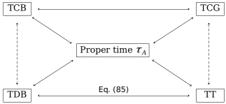
Figure 5: Various relativistic time-scales and their relations. Each of the coordinate time-scales TCB, TCG, TT and TDB can be related to the proper time $\tau_{A}$ of an observer $A$, provided that the trajectory of the observer in the BCRS and/or GCRS is known (Petit and Luzum, 2010). Dashed lines represent transformations with fixed rates, whereas full lines represent transformations that depend on the metric potentials, following to the IAU recommendations (Soffel, 2003).

The time-scales in the BCRS and GCRS are denoted by TCB and TCG, respectively (Soffel, 2003). The relation between TCB and TCG are given in Soffel (2003). At the Earth level, the Terrestrial Time (TT) has been defined in order to remain close to the realized atomic time (TAI). It differs from the TCG by a constant rate (Soffel, 2003).

Likewise, at the level of the solar system barycenter, the TDB is defined as a linear transformation of the TCB. The relations between the various time scales is shown in Fig. 5.

The difference between TT and TDB is produced by planetary ephemerides, by integrating the following equation together with the equations of motion (Klioner, 2008; Fienga et al., 2009)

$$\frac{d(TT-TDB)}{d(TDB)}= (L_{B}+\frac{1}{c_{2}}a)(1+L_{B}-L_{G})-L_{G}+\frac{1}{c_{4}}b,$$ (85)

with $L_{B}$ and $L_{G}$ are defining constants for TDB relatively to TCB and TT relatively to TCG, respectively (see i.e. Klioner (2008); Petit and Luzum (2010) for the full definition) and where

$$a= -\frac{1}{2}v_{T}^{2}-\sum_{A\neq T}\frac{\mu_{A}}{r_{AT}}\,$$

$$b= -\frac{1}{8}v_{T}^{4}+\frac{1}{2}\left[\sum_{A\neq T}\frac{\mu_{A}}{r_{AT}}\right]^{2}+\sum_{A\neq T}\frac{\mu_{A}}{r_{AT}}\Bigg{\{}4\bm{v}_{T}.\bm{v}_{A}-\frac{3}{2}v_{T}^{2}-2v_{A}^{2}$$

$$+\frac{1}{2}\bm{a}_{A}.\bm{r}_{AT}+\frac{1}{2}\left(\frac{\bm{v}_{A}.\bm{r}_{AT}}{r_{AT}}\right)^{2}+\sum_{B\neq A}\frac{\mu_{B}}{r_{BA}}\Bigg{\}},$$ (86)

following the notations of Eq. (84). In Park et al. (2021), terms related to the perturbations induced by the oblateness of the Sun were also added in the DE440 (TT-TDB) computation.
Finally, planetary observations are also related to time. Following the IERS conventions (Petit and Luzum, 2010), those observations obtained on the ground are given in UTC, related to TDB by TT and TAI. The observations obtained in other planetary systems (i.e. positions of a spacecraft orbiting Mercury) are, up to now, given also in UTC as the differences between the coordinate time defined for the corresponding planetary system (in the previous example, Mercury) and TDB or TT, are not significant at the present day accuracy. However, with missions such as Bepi-Colombo, it will be necessary to account for the local gravitational potential in the definition of the observational time scales (i.e Turyshev et al. (2013a); Nelson and Ely (2006); Milani et al. (2002)). In conclusion, it is important to keep in mind that the various measured proper times are converted beforehands into coordinate times—according to the laws of general relativity.

3.2.3 Inertial Frame

The coordinate frame of the planetary and lunar ephemerides is linked to the International Celestial Reference System (ICRS) by its current realization achieved by VLBI measurements of the positions of extragalactic radio sources (i.e., quasars) defined in the ICRF (Standish, 1998b). The planetary orbits are tied to ICRF because the observations used for their adjustment have been obtained in the ICRF. For the inner planets, the VLBI observations of Venus and Mars-orbiting missions give a tie with an accuracy better than the milliarcsecond (Fienga et al., 2011a; Folkner et al., 2014a). For the outer planets, the link is maintained with the same level of uncertainty thanks the VLBI observations of Juno and Cassini (Jones et al., 2019; Fienga et al., 2011a; Folkner et al., 2014a) orbiting Jupiter and Saturn, respectively. Some other methods have been investigated for enhancing the link between planetary ephemerides and ICRF. In particular, one can notice the use of Lunar Laser Ranging observations (Pavlov, 2020) and the use of GAIA DR2 asteroid positions (Deram et al., 2022). The tie between the planetary ephemerides frame and ICRF is confirmed to be sub-mas level accuracy in both approaches.

3.2.4 Definition of the solar system barycenter (SSB)

The definition of the solar system barycenter at the origin of the time of integration is based on the hypothesis of the conservation of the energy of the dynamical system composed by the planets, the Moon and the asteroids (including Trans-Neptunian Objects) in the solar system. The position $R$ and the velocity $V$ of the center of mass are then invariant. Using the notation of DE430 (Folkner et al., 2014b), it comes

$$\begin{cases}R=\frac{\sum_{i}\mu^{*}_{i}\bm{r}_{i}}{\sum_{i}\mu^{*}_{i}}=0\\ V=\frac{dR}{dt}=0\\ \end{cases}$$ (87)

where $\bm{r}_{i}$ and $\bm{v}_{i}$ being respectively its barycentric position and velocity vectors of the planet $i$. $\mu^{*}$ is given by

$$\begin{cases}\mu^{*}_{i}=\mu_{i}\left(1+\frac{v^{2}_{i}}{2c^{2}}-\frac{1}{2c^{2}}\sum_{j\neq i}\frac{\mu_{j}}{r_{ij}}\right)\\ \\ \dot{\mu}^{*}_{i}=\frac{\mu_{i}}{2c^{2}}\left(\sum_{j\neq i}\mu_{j}\frac{(\bm{r}_{j}-\bm{r}_{i}).(\bm{v}_{j}+\bm{v}_{i})}{r^{3}_{ij}}\right)\\ \end{cases}$$ (88)

with $\mu_{i}$ the product of the gravitational constant G with the inertial mass of the body $i$. The term $\dot{\mu}^{*}_{i}$ is not included in DE430 nor DE440 ephemerides (Folkner et al., 2014c; Park et al., 2021) but is accounted for in the INPOP ephemerides (Fienga et al., 2008). The positions and velocities of the SSB are then obtained by integration of the following equations and up to the c^-2 order,

$$\begin{cases}\sum_{i}\mu^{*}_{i}\bm{r}_{i}=0\\ \sum_{i}\mu^{*}_{i}\bm{v}_{i}+\dot{\mu}^{*}_{i}\bm{r}_{i}=0\\ \end{cases}$$ (89)

In the INPOP formalism (Fienga et al., 2008), Eqs. (89) and (88) are solved only at the initial step of the planetary integration and a constant vector in positions and velocities is subtracted to all the body positions and velocities for having $R$ and $V$ to 0. Once the frame is centered on the SSB defined by Eq. (89) at J2000 (inital date of integration for INPOP epehemerides), the equations of motion of the solar system bodies and of the Sun are integrated in this fixed frame. The method described here is used by the INPOP planetary ephemerides since INPOP08 (Fienga et al., 2008). In JPL DE430 ephemerides (Folkner et al., 2014a), the Sun initial coordinates are set up such as $R$ and $V$ are 0, the equations of motion of the Sun, the Moon, planets, and asteroids being then integrated in the fixed frame. In the former JPL DE versions, such as DE421 (Folkner et al., 2008), the Sun coordinates were set up at each step of integration for maintaining $R$ and $V$ to 0 all along the integration process. A description of the successive SSB implementations for older JPL versions can be found in Folkner et al. (2014a) and discussions concerning possible uncertainties are presented in Fienga et al. (2008) and Folkner et al. (2014a). It is interesting to note that, for the tests of the Equivalence Principle (sect. 4.2), $\mu_{i}$ of Eq. (89) and (88) will still correspond to the product of G with the inertial mass of the body. It will then differ from the gravitational mass used for computing the planetary acceleration as in Eq. (90).

3.3 The dynamical model

3.3.1 Point-mass interactions

In the context of Soffel (2003) and of the metric defined in Eq. (80) and (84), one can then, in the mass-monopole approximation, write the equations of motion of bodies as well as the conservation laws satisfied by the SSB as given in Damour and Vokrouhlický (1995). In BCRS, the equation of motion for the point-mass interaction is given by

$$\bm{a}_{T}= -\sum_{A\neq T}\frac{\mu_{A}}{r_{AT}^{3}}\bm{r}_{AT}$$

$$-\sum_{A\neq T}\frac{\mu_{A}}{r_{AT}^{3}c^{2}}\bm{r}_{AT}\Bigg{\{}v_{T}^{2}+2v_{A}^{2}-4\bm{v}_{A}.\bm{v}_{T}-\frac{3}{2}\left(\frac{\bm{r}_{AT}.\bm{v}_{A}}{r_{AT}}\right)^{2}$$

$$\hskip 85.35826pt-\frac{1}{2}\bm{r}_{AT}.\bm{a}_{A}-4\sum_{B\neq T}\frac{\mu_{B}}{r_{TB}}-\sum_{B\neq A}\frac{\mu_{B}}{r_{AB}}\Bigg{\}}$$

$$+\sum_{A\neq T}\frac{\mu_{A}}{c^{2}r_{AT}^{3}}\left[4\bm{r}_{AT}.\bm{v}_{T}-3\bm{r}_{AT}.\bm{v}_{A}\right](\bm{v}_{T}-\bm{v}_{A})$$

$$+\frac{7}{2}\sum_{A\neq T}\frac{\mu_{A}}{c^{2}r_{AT}}\bm{a}_{A}\,,$$ (90)

This equation is known as the Einstein-Infeld-Hoffmann-Droste-Lorentz (EIHDL) equation of motion, and it is numerically integrated for obtaining the modern planetary ephemerides in general relativity at the first post-Newtonian c^-2 level. Additional accelerations induced by the oblateness of the Sun (sect 3.3.4) or frame dragging effects (sect 3.3.3) are also accounted for in order to describe the motion of the planets at the level of accuracy required by the modern space mission observations. Other multipole moments than the Sun quandrupole moment are negligeable at the current level of accuracy.

3.3.2 Asteroid perturbations

Differences in the number of point-mass perturbations exist between planetary ephemerides. Table 2 summarizes them by splitting the case of the Main-Belt asteroids (MBA) on the one hand, and of the Trans-Neptunian objetcs (TNO) on the other hand. The problem of the modelisation of the MBA perturbations on the inner planet orbits has been addressed since DE405 (Standish, 2001). The issue is that there is a considerable number of objects (at least 250,000), for which the masses are unknown, that can potentially interact gravitationally with the inner planets (mainly Mars). With DE405 (Standish, 1998a), 5 asteroids (Ceres, Pallas, Vesta , Iris and Bamberga) have been identified as the main perturbers associated with an averaging of the effect induced by the rest of the MBA based on taxonomic classifications. But this modelisation shows its limits with the improvement of the accuracy of the Mars-orbiter tracking data (Standish and Fienga, 2002). Williams (1984) proposed a list of 343 individual objects among the MBA gathering the most perturbing asteroids to consider for the construction of accurate planetary ephemerides. That list has been confirmed by Kuchynka and Folkner (2013) and since DE430 this is the Williams (1984) objects that are taken into account in DE and INPOP planetary ephemerides, with their masses individually fitted to observations together with the initial conditions of planet orbits, the mass of the Sun and the Earth-Moon mass ratio (Folkner et al., 2014a; Fienga et al., 2019b). A detailed description of the complexity of such an adjustment is out of the scope of this review but more comments on the accuracy obtained for these mass determinations can be found in Kuchynka and Folkner (2013) and Fienga et al. (2020a). In order to overcome this problem, but also to reduce the time cost of integrating an important number of objects, it has been proposed to substitute or to complement the MBA individual point-mass contribution by a global ring potential.

The first ring modelisation was proposed by Krasinsky et al. (2002) as a static ring fixed at 2.8 AU from the SSB. An updated model maintaining the total linear and angular momenta of the system has been implemented in Fienga et al. (2009) and Kuchynka et al. (2010) as a way to account for additional MBA contribution associated with a shorter list of individual point-mass perturbers. This approach has not be retained for MBA in DE (Folkner et al., 2014a) and INPOP (since INPOP13c (Fienga et al., 2014)) ephemerides but kept in EPM ones associated with individual mass and density determinations for 3 classes of MBA (Pitjeva and Pitjev, 2018).

After the introduction of the Juno and Cassini tracking data, it became clear that the perturbations induced by the TNO have to be included in the model. In Pitjeva and Pitjev (2018); Di Ruscio et al. (2020b) and Park et al. (2021), individual point-mass perturbations of the most massive and binary Trans-Neptunian objects have been added together with a circular ring for accounting for the average effect of the rest of the TNO. However as the TNO orbits are more eccentric than the MBA ones, Fienga et al. (2021a) had introduced, instead of a circular ring, 500 individual point-mass TNO perturbers with observed orbits but of equal mass. This latest assumption simplifies the adjustment as only one parameter (the total mass spread over 500 objects) is used and fitted for characterising the TNO perturbations.

The full 1PN general relativity equation of motion is only taken into account for the first biggest MBA (Ceres, Pallas, Vesta , Iris and Bamberga). For the rest of the MBA and the TNO point-mass interactions, the perturbations on the planet orbits, and on the other asteroid orbits, are estimated at the Newtonian level only. This is done in order to reduce the computational cost, but it is consistent with the overall PN perturbative approach—given that those perturbations are already very small at the Newtonian level, such that their contributions at the post-Newtonian level are negligible.

3.3.3 Lense-Thirring acceleration

The Lense-Thirring (LT) acceleration induced by the Sun rotation has been recently added in modern planetary ephemerides (Pitjeva and Pitjev, 2018; Park et al., 2021; Fienga et al., 2021b) . Its new introduction is justified by the accuracy reached by space missions, especially those close to the Sun and Mercury such as Messenger and Bepi-Colombo (Genova et al., 2018). It also has been shown that it helps for disentangling the PPN parameters for their contribution to the planetary motions (Fienga et al., 2021a).

In 2011, Iorio et al. (2011) has also shown that this effect contributes to about 10$\%$ of the dynamical acceleration induced by the shape of the Sun in General relativity (see sect. 3.3.4). The acceleration induced by the Lense-Thirring effect generated by a central body (here the Sun) at the first post-Newtonian approximation is given by

$$\bm{a}_{LT}=\frac{2GS}{c^{2}r^{3}}\left[\frac{3\bm{k}.\bm{r}}{r^{2}}(\bm{r}\wedge\bm{v})-(\bm{k}\wedge\bm{v})\right]$$ (91)

where $G$ is the gravitational constant, $c$ the speed of light, $\bm{S}$ is the Sun angular momentum such as $\bm{S}=S\,\bm{k}$ where $\bm{k}$ is the direction of the Sun rotation pole defined according to the IAU right ascension and declination (Archinal et al., 2018), $\bm{r}$ and $\bm{v}$ are the position and velocity vectors of the planet relative to the Sun and $\gamma$ is the PPN parameter for the light deflection, equal to 1 in general relativity. The Lense-Thirring effect hence depends on the Sun angular momentum, $\bm{S}$ that can be obtained by considering different models for the Sun rotation including both the rotation of the convective region well constrained by helioseismology and the rotation of the Sun core (see Fienga et al. (2021a) for discussion).

3.3.4 Shape of the Sun

Among the solar multipole moments, only the degree 2 order 0 term of the spherical harmonic decomposition of the Sun gravity field, J${}_{2}^{\odot}$—which is identified to the oblateness of the Sun— leads to a significant impact on the planetary ephemerides at the current level of accuracy. The J${}_{2}^{\odot}$ induces an acceleration $\bm{a}_{J_{2}^{\odot}}=({a}^{x}_{J_{2}^{\odot}},{a}^{y}_{J_{2}^{\odot}},{a}^{z}_{J_{2}^{\odot}})$ to be added to EIHDL Eq. (90) such as (Sharma et al., 2016; Ivashkin, 2021) :

$$\begin{cases}{a}^{x}_{J_{2}^{\odot}}=&-\frac{3}{2}\mu_{\odot}J_{2}^{\odot}R^{2}_{\odot}x\frac{(x^{2}+y^{2}-4z^{2})}{2r^{7}},\\ {a}^{y}_{J_{2}^{\odot}}=&-\frac{3}{2}\mu_{\odot}J_{2}^{\odot}R^{2}_{\odot}y\frac{(x^{2}+y^{2}-4z^{2})}{2r^{7}},\\ {a}^{z}_{J_{2}^{\odot}}=&-\frac{3}{2}\mu_{\odot}J_{2}^{\odot}R^{2}_{\odot}z\frac{(3x^{2}+3y^{2}-2z^{2})}{2r^{7}}\end{cases}$$ (92)

where $\mu_{\odot}$ and R_⊙ are the gravitational parameter and the radius of the Sun, respectively, $r$ is the heliocentric distance of the planet, $(x,y,z)$ being its heliocentric coordinates.

It is common to see in the literature dealing with geodesy and geophysics the contribution of J${}_{2}^{\odot}$ as time variations of the osculating elements of the perturbed orbit such as (Kaula, 1966; Bertotti et al., 2003a):

$$\begin{cases}\dot{a}=\,0\mathchar 24635\relax\;&\dot{e}=\,0\mathchar 24635\relax\;\dot{i}=\,0\\ \dot{\omega}=&\frac{3}{4}J_{2}^{\odot}\frac{n}{(1-e^{2})^{2}}\frac{R^{2}_{\odot}}{a^{2}}(5\,\cos^{2}i-1)\\ \dot{\Omega}=&-\frac{3}{2}J_{2}^{\odot}\frac{n}{(1-e^{2})^{2}}\frac{R^{2}_{\odot}}{a^{2}}\cos i\\ \dot{M}=&n+\frac{3}{4}J_{2}^{\odot}\frac{n}{(1-e^{2})^{3/2}}\frac{R^{2}_{\odot}}{a^{2}}(3\,\cos^{2}i-1)\\ \end{cases}$$ (93)

with $a$, $e$, $n$ and $i$ are the semi-major axis, the eccentricity, the mean motion and the inclination of the planetary orbit impacted by the oblateness of the Sun. $M$ is the planet mean anomaly. We give these equations Eq. (93) as a simple illustration of the type of contribution one may get from the Sun quadrupole. It is then clear that the major contribution of this quadrupole term is on the advance of nodes $\dot{\Omega}$ and perihelia $\dot{\omega}$ of the planetary orbits. This system of equations is also somehow useful to apprehend the potential correlations that may appear between the Sun quadrupole moment and the semi-major axis and eccentricity.

Fig 6 shows $J_{2}^{\odot}$ values deduced from planetary ephemerides including or not the Lense-Thirring contribution. It is clear, from this Figure, that the introduction of the Lense-Thirring acceleration in the model improves significantly the $J_{2}^{\odot}$ determinations. The values obtained with LT (Fienga et al., 2021a; Park et al., 2017) are indeed closer to the ones issued from helioseismologic surveys (Pijpers, 1998; Antia et al., 2008) than those obtained before the LT introduction (Fienga et al., 2019b; Iorio et al., 2011; Viswanathan et al., 2017; Fienga et al., 2014; Folkner et al., 2014a; Fienga et al., 2011a, 2009). In general relativity, the difference in $J_{2}^{\odot}$ with or without LT is of about about 7 to 10 $\%$ .

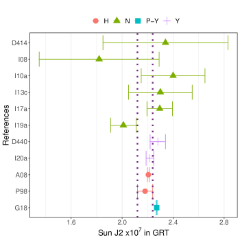
Figure 6: Values of the Sun oblateness $J_{2}^{\odot}$ obtained with different ephemerides and other methods in the general relativity frame. H stands for values deduced from helioseismology, P points values obtained in a partial fit of planetary orbits (i.e. considering only a couple of planets for the fit, like Mercury and the Earth), N indicates values obtained before the introduction of the Lense-Thirring acceleration in the dynamical modeling and Y gives the values obtained after the introduction. The dotted lines give the limits of the less constraining helioseismologic value from Pijpers (1998). In y-axis, are given the references : G18 is Genova et al. (2018), P98 Pijpers (1998), A08 Antia et al. (2008), I20a Fienga et al. (2021a), D440 Park et al. (2017), I19a Fienga et al. (2019b), I17a Viswanathan et al. (2017), I13c Fienga et al. (2014), D414 Konopliv et al. (2006), I10a Fienga et al. (2011a) and I08 Fienga et al. (2009). It is important to note that in Genova et al. (2018), only the orbit of Mercury is considered.

As it will be developed in sect. 4.1, the introduction of gravity theories that are different but close to general relativity induces modifications of the previous Eqs. (90-92). In this context, the value of $J_{2}^{\odot}$ can also be determined with planetary ephemerides in the PPN framework, like given in Table 5 . But we will see that the value of $J_{2}^{\odot}$ can be strongly correlated to the value of non-general relativity parameters, and in particular the PPN parameter $\beta$ (Milani et al., 2002)—as one can get an intuition from Eq. (100). In sect. 4.1, we will see that the determination of the Sun oblateness when one includes PPN deviations plays a key role in the context of the global adjustment of planetary ephemerides .

Table 3: Detailed example of a planetary ephemeris (here INPOP21a) data sample extracted from (Fienga et al., 2021b). Column 1 gives the observed planet and information on the type of observations, Column 2 gives the type of data or the name of spacecraft used for producing the data. Columns 3 and 4 give the time interval and the a priori uncertainties provided by space agencies or the navigation teams, respectively. In Column 2, $MRO$ for Mars Reconnaissance Orbiter and $MO$ for Mars Orbiter. Flybys stands for average normal points obtained during a flyby of a spacecraft with $U,C,P,V$ gives the normal points obtained after the flybys of Ulysses, Cassini, Pionneer and Voyager respectively. $radar$ is for direct radar ranging on planetary surfaces, $VLBI$ stands for Delta-DOR observations and $Transit+CCD$ gives the optical angular observations obtained by transit, photographic plates or CCD. $H14$ stands for Hees et al. (2014b).

Planet / Type [unit]	s/c or method	Period	Averaged
			Accuracy
Mercury
Direct range [m]	Surface	1971.29 : 1997.60	900
Radio Science range [m]	Messenger	2011.23 : 2014.26	5
Navigation range [m]	Mariner	1974.24 : 1976.21	100
Venus
VLBI [mas]	Magellan, Venus Express	1990.70 : 2013.14	2.0
Direct range [m]	Surface	1965.96 : 1990.07	1400
Navigation range [m]	Venus Express	2006.32 : 2011.45	7.0
Mars
VLBI [mas]	MGS, MRO	1989.13 : 2013.86	0.3
Navigation range [m]	Mars Express	2005.17 : 2019.37	2.0
Radio Science range [m]	MGS	1999.31 : 2006.70	2.0
Radio Science range [m]	MRO/MO	2002.14 : 2014.00	1.2
Navigation range [m]	Viking	1976.55 : 1982.87	20.0
Jupiter
VLBI [mas]	Galileo	1996.54 : 1997.94	11
	Juno	2016:2020	0.5
Optical RA/Dec [arcsec]	Transit+CCD	1924.34 : 2008.49	0.3
Flyby RA/Dec [mas]	U,C, P, V	1974.92 : 2001.00	8.0
Flyby range [m]	U,C, P, V	1974.92 : 2001.00	2000
Radio Science range [m]	Juno	2016.65 : 2020.56	20
Saturn
Optical RA/Dec [arcsec]	Transit+CCD	1924.22 : 2008.34	0.3
VLBI RA/Dec [mas]	Cassini	2004.69 : 2017.9	0.6
JPL H14 [m]	Cassini	2004.41 : 2014.38	25.0
Navigation [m]	Cassini	2006.01 : 2009.83	6.0
Radio Science : Titan Flybys [m]	Cassini	2006.01 : 2016.61	15.0
Radio Science : Grand Finale) [m]	Cassini	2017.35 : 2017.55	1.0
Uranus
Optical RA/Dec [arcsec]	Transit+CCD+photo	1924.62 : 2013.75	0.25
Flyby RA/Dec [mas]	Voyager	1986.07	50
Flyby range [m]	Voyager	1986.07	50
Neptune
Optical RA/Dec [arcsec]	Transit+CCD+photo	1924.04 : 2007.88	0.3
Flyby RA/Dec [mas]	Voyager	1989.65	15.0
Flyby range [m]	Voyager	1989.65	2

3.4 Planetary Datasets

The modern planetary ephemerides are characterised by the role of planet positions deduced from spacecraft missions either by navigation tracking or by the use of radio science data. In both cases, it is the distance between a station on the ground and a spacecraft orbiting of flying over a planet that is used for the construction of planetary ephemerides. The angular position between the same spacecraft and an extra-galactic source (generally a reference beacon for the construction of the inertial frame, ICRF) is also of great importance for the adjustment of the planetary ephemerides as it allows the tie of the planetary planes to the ICRF (see sect. 3.2.3). Optical meridian transit and CCD angular positions are mainly kept for the constraint on the outer planet orbits. A full description of the different data sets used for the construction of the planetary ephemerides can be found in Folkner et al. (2014a) and Fienga et al. (2009) and regular updates are presented for every new releases such as for DE440 (Park et al., 2021) or INPOP19a (Di Ruscio et al., 2020b). Table 3 gives the different data sets used for the construction of INPOP21a (Fienga et al., 2021b), counting a total of about 200,000 observations, this number of course varying from one ephemeris to another. Very similar datasets have been used by DE440 (Park et al., 2021).

3.4.1 Time delay of the propagation of light

The propagation of light is affected by the curvature of spacetime. Although the trajectory of light is bent in gravitational potentials, this bending is negligible for radio science in the solar system, and the main effect is known as the Shapiro delay: the propagation time between two points is not simply the Euclidean BCRS distance over the speed of light between an emission point $e$ and a reception point $r$, but it also involves a delay in general relativity that depends on the gravitational potentials as follows (Moyer, 2000)

$$c(t_{r}-t_{e})_{GRT}=R+\sum_{A}2\frac{\mu_{A}}{c^{2}}\ln\frac{\bm{n}\cdot\bm{r}_{rA}+r_{rA}+\frac{4\mu_{A}}{c^{2}}}{\bm{n}\cdot\bm{r}_{eA}+r_{eA}+\frac{4\mu_{A}}{c^{2}}}\,,$$ (94)

where the $R$ is the Euclidean coordinate distance, $\bm{n}=(\bm{r}_{r}-\bm{r}_{e})/\|\bm{r}_{r}-\bm{r}_{e}\|$, $\bm{r}_{iA}=\bm{r}_{i}-\bm{r}_{A}$ and $r_{iA}=\|\bm{r}_{iA}\|$ with $i=e$ or $r$. Note that Eq. (94) slightly differs from the actual Shapiro equation through the $c^{-2}$ terms in the logarithm function. It has lately been realized that this version of the Shapiro delay—rather than the usual equation without the additional $c^{-2}$ terms in the logarithm—allows to account for the so-called second order time propagation enhanced terms, which can become numerically significant for particular conjunction situations despite formally being next-to-leading-order (or $c^{-4}$) terms (Ashby and Bertotti, 2010; Linet and Teyssandier, 2016). In practice, the difference between the two versions of the Shapiro delay is irrelevant for current planetary ephemerides.

However, it has been realized during the last decade that for close solar conjunctions, additional enhanced $c^{-4}$ terms may no longer be negligeable, in particular for BepiColombo MORE (Mercury Orbiter radio science Experiment) (Hees et al., 2014a; Cappuccio et al., 2021) measurements. As a consequence, for close conjunction events, one might have to go beyond Eq. (94) and use a full second order time propagation time formula. This will be challenging in many different ways —see Appendix A. For planetary ephemeris construction, Bepi-Colombo MORE experiment should provide range measurements up to close to 5^∘ to the Sun, that is, close to conjunction (Fienga et al., 2021a). For such close-to-the-Sun observations, a specific analysis will have to be done in order to account for the neglected terms of Eq. (94), but in the framework defined by the IAU (harmonic gauge).

In any case, when one deals with an alternative theory of gravity, one has to take care of the consistency between the different levels of construction of the ephemeris: modifying the Shapiro delay or the equation of motion for massive bodies is not without consequences on the other.

3.4.2 Radio science and navigation data

This type of data represent more than 65$\%$ of the full data sample used for the construction of the planetary ephemerides. It gathers measurements of distances in terms of time delays obtained during orbital or flyby phases of space missions, either during the regular navigation process, or during specific scientific sessions dedicated to radio science experiments. In this latter case, a detailed assessment of the capabilities of the radio transpondeur used for the re-emission of the captured signal is needed for the analysis (see i.e. Cappuccio et al. (2020)). The measurement is the time differences between the time of emission of the signal by a ground-based antenna, the time of capture by the transponder on board of a spacecraft, the time of re-emission by this transponder after amplification and the time of reception of the transmitted signal by the same or a different ground-based antenna. Using a known orbit of the spacecraft around or near the planet, it is then possible to deduce the planetary range measurement, by accounting for the distance between the spacecraft and the centre of mass of the planet estimated during the s/c orbit determination. The accuracy of the range constraints deduced from the radio science and navigation data is then strongly dependant on the uncertainties of the spacecraft orbit determination.

The distribution of the data per missions is given in Fig. 7. In numbers, the Mars orbiter observations dominate, followed by the Venus tracking data. In terms of accuracy, the Mars data also lead the fit together with the less numerous but important tracking data of the Juno mission orbiting Jupiter as well as the Cassini radio science and tracking data for Saturn. The predominance in numbers and accuracy of the Mars observations on the planetary ephemerides data sample explain why some tests of general relativity have been said to be driven by the Mars orbit (Will, 2018a), whereas Bernus et al. (2019) stressed also the importance of the outer planet radio science experiments.

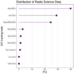
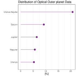
Figure 7: Example of distribution in percentages of the radio science and tracking data and the optical observations. On the left-hand side, data samples are identified by planets (Ma stand for Mars, Me for Mercury, Ve for Venus, Ju for Jupiter, Sa Saturn and UN for Uranus and Neptune) and by missions. On the right-hand side, the data sample are identified according to the observed planet. A specific tag is made on the set of astrometric positions obtained by Camargo et al. (2022). The presented datasets correspond to the one of INPOP21a (see Table 3). Roughly similar distribution is present for DE and EPM ephemerides.

Furthermore, in term of gravitational framework, these observations are also given in the framework used for studying the motion of the spacecraft around the planet. This framework is usually general relativity and discussions have been held regarding the consistency of testing alternative theories of gravity with observational constraints obtained in general relativity (i.e. Verma et al. (2014)). The most simple way to solve this problem is to operate the spacecraft orbit determination (OD) in the same framework as the one of the alternative theories to be tested. But as the s/c navigation is regularly interrupted, even during orbital phases, by engine boosts or attitude corrections, introducing significant changes in the orbit, OD is usually done over a short duration of time (from few hours to few days), in between these manoeuvres. Most of the time, up to now, alternative theories of gravity start to significantly differ from general relativity over longer time intervals. But it is clear that with the increase of the accuracy in the s/c orbit tracking, the modified general relativity that one wants to test should also be implemented during the OD process. See for example De Marchi and Cascioli (2020).

In parallel to the radar tracking, navigation teams also acquire positions of the spacecraft relative to extra-galactic sources by using facilities also dedicated to VLBI observations. This type of observations, called Delta -DOR, represent less than 1 $\%$ of the full data sample but they are crucial for linking the ephemeris reference frame to the ICRF (see sect. 3.2.3). The first were obtained in 1981 (Donivan and Newhall, 1981) with the Viking Mars lander. Technical description related to the production of this type of observations can be found in Folkner et al. (1994) and Moyer (2000). The most recent planetary ephemerides account for a total of about 300 VLBI positions, mainly extracted from the tracking data of Mars, Venus, Jupiter and Saturn orbiters with accuracies about less than 1 milliarcsecond of degree (mas) (Jones et al., 2011, 2019; Park et al., 2021).

3.4.3 Angular ground-based observations

Finally, the observational data base is completed by the optical observations of outer planets. This set constitutes about 35$\%$ of the full data sample, and, despite their uncertainties, are crucial for Uranus and Neptune. For these two planets, only 1 flyby per planet has been acquired during the Voyager missions, leading to a weak constraint for several decade-long orbits. Direct transit observations of planets or satellites are part of the optical data samples as well as astrometric positions deduced from CCD observations and photographic plates. Both planet and satellite positions are included. In the case of satellite astrometry, the position of the planetary barycenter is deduced using satellite ephemerides (i.e. Camargo et al. (2022)). The long-term (several decades) behaviour of outer planet orbits is then driven by the planet barycenter equation of motion as given in Eq. (96), but also by the satellite dynamics. Additionally, depending on the reference frames used for the data publications, different algorithms are applied for transforming the astrometric positions (for example given in FK3, FK4 or FK5) to ICRF. Such transformations guarantee, at the level of accuracy of the optical data (about 50 to 100 mas), the link between the INPOP outer planet frame and ICRF. VLBI observations enforce this link at the VLBI accuracy which means a factor of at least 100 compared to the optical tie. On Fig. 7 are given an example (for INPOP21a) of the percentages of optical observations per planet. A specific tag is made on the data sample provided by Camargo et al. (2022) who did a new reduction of astrometric long-term observations of the Uranian main satellites obtained at the Pico dos Dias from 1982 to 2011, using the Gaia EDR3 as reference.

3.5 Fitting procedures

The main construction of planetary ephemerides uses a classic least squares approach. The total number of fitted parameters can be found in Table 2. It changes from one ephemeris to an other, depending the perturbations included in the model and the observational parametrizations required for the data analysis. Thus, to the parameters presented in Table 2, spacecraft bias accounting for additional transpondeur delays or additional ground-station delays (Kuchynka et al., 2012) have also to be added as well as parameters related to solar plasma corrections (Verma et al., 2013; Pitjeva et al., 2021).
Complementary methods have been proposed to make accuracy assessments, to overcome the problems of high correlated parameters, in particular in the frame of testing alternative theories of gravity (see sect 4.1), or of multiple correlations between parameters, as in the case of the determination of asteroid masses (Fienga et al., 2020a). In the context of computing threshold values for the violation of general relativity, Fienga et al. (2015) had tested genetic algorithm approaches for identifying sets of parameters (PPN $\beta$, $\gamma$, the Sun oblateness J${}_{2}^{\odot}$ and secular variations of the gravitational mass of the Sun, $\dot{\mu}/{\mu}$) with which planetary ephemerides can be computed and fitted to the observations with an comparable accuracy to the ephemeris (in this case INPOP15a) built in general relativity. Different approaches based on $\chi^{2}$ analysis with fixed PPN or alternative theory parameters have been investigated as well, using random walk exploration methods associated with various cost functions (Bernus et al., 2019, 2020, 2022; Fienga et al., 2021a). These methods have in common to be very conservative and to give larger constraints than those obtained with the least square procedures. See sect. 4.1 for the full discussion.

A final but important comment is about the masses used for the construction of the ephemerides.

Most of the planetary masses are not obtained during the construction of the planetary ephemerides but during the orbit determination of one or several spacecraft flying in planetary systems (see Table 4). They are obtained by combination of data from different missions and techniques, usually in the general relativity framework. For example, in the case of Neptune and Uranus, it is even a combination of Voyager radio tracking data, ground-based optical observations and images acquired by the s/c that leads to the determination of the mass of the planetary system. The s/c orbit and gravity field (mass) determinations are complex as they depend on various sources of interactions from solar radiation pressure, atmospheric dragging, maneuver residual accelerations to non-stochastic accelerations. For that reason, these s/c orbit and gravity field determinations are usually done independently from the planetary ephemerides. These masses are therefore obtained in the framework of the s/c orbit and of the gravity field determination algorithm, which assumes generally general relativity. Only, the gravitational mass of the Sun, the ratio between the mass of the Earth and the mass of the Moon (invariant to any change of the gravitational constant) as well as a variable number of asteroid gravitational masses (see sect. 3.3.2) are, in fact, estimated during the planetary ephemeris adjustment. In the case of a test of the violation of the Equivalence principle, the fact that some of the masses used in the ephemeris are obtained in the general relativity framework can introduce an inconsistency in the method. In principle, it should be necessary to consider a more global approach, including the s/c orbit determination in the same framework than the one of the planetary ephemeris. So far, such an attempt was only operated for Parametrized post-Newtonian tests (see sect. 4.1).

Table 4: Planetary masses used in DE440 (Park et al., 2021) and INPOP19a (Fienga et al., 2021b). Are indicated from which missions the masses were extracted from with the corresponding references.

Planet	References	Mission
Mercury	Konopliv et al. (2020)	Messsenger
Venus	Konopliv et al. (1999)	MAGELLAN
Mars	Konopliv et al. (2016)	MRO, MGS, Odyssey,
		Pathfinder, MER, Viking
Jupiter barycenter	Durante et al. (2020)	Juno + 5 s/c flybys +
	Jacobson (2021b)	ground-based and s/c optical data
Saturn barycenter	Jacobson (2021a)	Cassini + ground-based +
	Di Ruscio et al. (2020a)	s/c optical data
Uranus barycenter	Jacobson (2014)	Voyager 2 + ground-based optical data
Neptune barycenter	Jacobson (2009)	Voyager + ground-based and s/c optical data

4 Tests of alternative theoretical frameworks with planetary ephemeris

Thanks to the accuracy of the most recent observations but also to the more than one century long data span, planetary ephemerides are excellent tools for testing general relativity and its alternatives. In principle, if the model of gravity is not accurate enough, or does not well represent the physics as seen by the observations, it should then lead to a deterioration of the differences (residuals) between observed and computed quantities—deduced from the ephemeris. When the deterioration of residuals built with an alternative theory becomes statistically significant with respect to the residuals obtained in the general relativity framework, one can say that it disfavors the alternative theoretical framework—or favors general relativity over its alternative. On the opposite, if the residuals obtained with an alternative theory are significantly improved—that is, if there are significantly smaller—in comparison to the one obtained in the general relativity framework, it favors the alternative theory. However, so far, this has never occurred.

In the following sections, we will explore various theories or phenomenologies that have been scrutinized using planetary ephemerides. The selection of certain theories or phenomenologies to test, rather than others, can be driven by several considerations. One of them could be the historical circumstances. For example, the Parametrized Post-Newtonian (PPN) framework was developed during the early stages of the general relativity testing era and has since been widely employed in tests involving planetary ephemerides.

Another factor could be the complexity of the task, both in terms of numerical computations and statistical methodology. The larger the number of parameters to constrain a theory has, the larger the dimension of the theoretical space there is to examine. Additionally, there is an increasing risk of introducing multiple correlations between the parameters of the theory, as well as between these parameters and those of the solar system (i.e., masses). Given that it can take up to eight hours of computation to adjust the solar system parameters of the ephemeris at a single point in the parameter space (Mariani et al., 2023), achieving a densely filled parameter space becomes highly computationally demanding if the parameter space dimension is greater than one. Moreover, the statistical methodology also grows more complex with an increase in the number of parameters to constrain.

There is also the risk of missing a genuine detection—that is, obtaining better residuals in an alternative theory than in general relativity for a specific parameter value—if the parameter space of alternative theories explored is too sparsely populated. Therefore, it is of paramount importance to have a densely filled parameter space, which consequently makes computational time requirements escalate with the number of parameters to constrain. In the case of a classic least square approach, the risk of high correlations between parameters associated with the observational uncertainties also limit the possible theories to be tested. As a result, tests are often conducted on theories or phenomenologies that hinge on few parameters only.

4.1 Parametrized post-Newtonian framework

For metric theories—that is, theories for which the additional gravitational fields do not couple to matter directly, such that the theories satisfy the weak equivalence principle by design—all the differences with respect to general relativity can be taken into account through parameters that appear in front of the gravitational potentials in the metric (Will, 2014, 2018b). Indeed, because the weak equivalence principle is enforced by hand by imposing that the additional gravitational fields do not couple to matter directly, particles still follow geodesics of the metric and proper time is still defined from the metric only.

Many theories then turn out to generate the same type of metrics, where the differences with respect to general relativity can be parametrized by a set of a few parameters in the metric only—which values depend upon the theory considered. This comes in handy, as it allows to derive all the equations necessary in planetary ephemerides—that are, the time-scale definitions, the motion of celestial bodies and the Shapiro delay—from a single original parametrized metric. This whole framework is therefore called the parametrized post-Newtonian (PPN) formalism.

Nevertheless, as it will be discussed in Sec 4.1.2, the coordinate system being used for planetary ephemerides matters, and one has to make sure that the coordinate system being used for alternative theories is compatible at the required level of accuracy with the IAU standards used to convert observables (e.g. the roundtrip of an electromagnetic signal measured in terms of the proper time of the local clock) into spatial and temporal coordinate positions (e.g. the distance of a spacecraft with respect to the ground-based station being used).

Table 5: PPN parameters $\beta$ and $\gamma$ obtained with planetary ephemerides. Columns 1,2 and 3 give respectively the reference, the ephemeris involved and method used. As explained in the text (sect. 4.1), we consider a classification based on 3 types of adjustment methods: the direct least square fit combining $\beta$, $\gamma$, all the ephemeris parameters and the oblateness of the Sun, J${}_{2}^{\odot}$ (FF), the partial fit where some parameters are fixed such as $\gamma$ or J${}_{2}^{\odot}$ and the other are fitted (PF), the random walk exploration (RW) where $\beta$ and $\gamma$ are randomly sampled when the rest of the parameters (including J${}_{2}^{\odot}$) are fitted. Are given for information the results obtained in considering only the Mercury orbit (MSG).

Reference	PE	Method	$\beta-1$	$\gamma-1$	J${}_{2}^{\odot}$
			$\times$ 105	$\times$ 105	$\times$ 107
(Pitjeva, 2001)	EPM2000	FF	40 $\pm$ 20∗	10 $\pm$ 10∗	2.43 $\pm$ 0.67∗
(Standish, 2001)	DE405	FF	10 $\pm$ 10 ∗	40 $\pm$ 10∗	2.46 $\pm$ 0.68∗
(Pitjeva, 2005b)	EPM2004	FF	0 $\pm$ 10 ∗	-10 $\pm$ 20 ∗	1.9 $\pm$ 0.3
(Fienga et al., 2009)	INPOP08a	PF	7.5 $\pm$ 12.5	0.0	fixed to 1.82
(Fienga et al., 2011a)	INPOP10a	PF	-4.1 $\pm$ 7.8	-6.2 $\pm$ 8.1	fixed to 2.40
(Konopliv et al., 2011)	DE421	PF	4 $\pm$ 24	fixed to 2.1	fixed to 1.8
(Pitjeva and Pitjev, 2013)	EPM2011	FF	-2 $\pm$ 3	4 $\pm$ 6	2.0 $\pm$ 0.20
(Verma et al., 2014)	INPOP13c	FF	0.2 $\pm$ 2.5	-0.3 $\pm$ 2.5	2.40 $\pm$ 0.20
(Fienga et al., 2015)	INPOP15a	FF	-6.7 $\pm$ 6.9	-0.8 $\pm$ 5.7	2.27 $\pm$ 0.25
(Fienga et al., 2015)	INPOP15a	RW	0.00 $\pm$ 6.90	-1.55 $\pm$ 5.01	2.22 $\pm$ 0.13
(Park et al., 2017)	DE440	PF	-2.6 $\pm$ 3.9∗	fixed to 2.1	2.25 $\pm$ 0.09∗
(Genova et al., 2018)	DE438	MSG	-1.625 $\pm$ 1.8	fixed to 2.1	2.246 $\pm$ 0.02
(Fienga et al., 2021a)	INPOP20a	PF	1.9 $\pm$ 6.28	2.64 $\pm$ 3.44	2.165 $\pm$ 0.12
(Fienga et al., 2021a)	INPOP20a	RW	-1.12 $\pm$ 7.16	-1.69 $\pm$ 7.49	2.206 $\pm$ 0.03

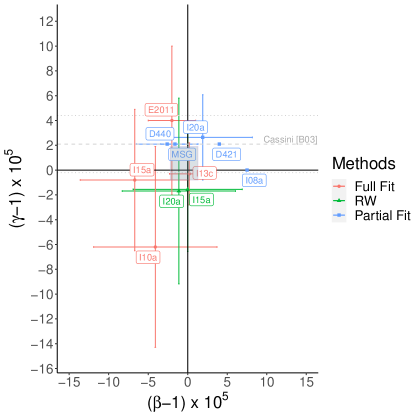
Figure 8: Constraints on PPN parameters $\beta$ and $\gamma$ obtained from planetary ephemerides as presented in Table 5. The shadded area is the zone common to all the constraints. The lightgrey lines give the constraint on $\gamma$ extracted from the Cassini experiment (Bertotti et al., 2003b). Three categories are considered: the values obtained from a full global fit, the one obtained using random walk exploration methods (RW) and finally, the one constrained either in fixing one of the two parameters (usually $\gamma$ like in (Konopliv et al., 2011; Park et al., 2017)) either in considering only one planetary orbit (like the Mercury orbit for Genova et al. (2018) . These categories were labelled according to the Column 3 of Table 5 and the annotated text refers to Column 2 of Table 5.

Among the 10 PPN parameters discussed in Will (2014) and Will (2018b), we shall first only consider the Eddington-Robertson-Schiff parameters $\gamma$ and $\beta$, because most of the planetary ephemerides to this date focused on those parameters. A complete description of the PPN parameters will be discussed in Sec. 4.1.4. Let us write the metric as follows (Klioner and Soffel, 2000)

$$g_{00}= -1+\frac{2w}{c^{2}}-\frac{2\beta w^{2}}{c^{4}}+\mathcal{O}(c^{-5})$$

$$g_{0i}= -\frac{(4\gamma+3)}{2}\frac{w_{i}}{c^{3}}+\mathcal{O}(c^{-4})$$

$$g_{ij}= \delta_{ij}\left(1+\frac{2\gamma w}{c^{2}}\right)+\mathcal{O}(c^{-3})\,,$$ (95)

In general relativity, the PPN parameters $\beta$ and $\gamma$ equal to one, but not for alternative theories in general.

The form of the metric given in Eq. (95) is not sufficient in order to completely fix the coordinate system, and one has to impose an additional constraint (or gauge) in order to specify the metric field equations—see, e.g., Klioner and Soffel (2000). Since the IAU recommends the coordinates (or gauge) to be harmonic for general relativity (Soffel, 2003), it seems relevant to consider harmonic coordinates for alternative theories as well, such that (at least) the coordinate systems of the alternative theory reduce to the IAU coordinate systems in the limit for which both theories cannot be distinguished at the level of accuracy of the observations.

Ambiguity of the definition of harmonic coordinates

The very definition of what one may call harmonic coordinates can be ambiguous for alternative theories of gravity. For instance, for scalar-tensor theories, one can impose the usual post-Newtonian harmonic conditions—$g^{\alpha\beta}\Gamma^{0}_{\alpha\beta}=0$—either in the Jordan frame, or in the conformal Einstein frame (Damour and Esposito-Farese, 1992; Kopeikin and Vlasov, 2004; Minazzoli and Chauvineau, 2011; Will, 2018b; Kopeikin, 2019). But both choices reduce to the general relativity harmonic coordinate in the limit for which the difference between general relativity and the scalar-tensor theory becomes negligeable (e.g. for the Brans-Dicke parameter that is such that $\omega\rightarrow\infty$). Imposing the harmonic conditions in the Einstein frame has been shown to lead to more convenient properties (Damour and Esposito-Farese, 1992; Kopeikin and Vlasov, 2004; Minazzoli and Chauvineau, 2011; Kopeikin, 2019), notably with respect to the full theory of reference frames (Kopeikin and Vlasov, 2004). However, this definition of harmonic coordinates then becomes theory-dependent (Will, 2018b). In order to alleviate the ambiguity, Kopeikin and Vlasov (2004); Kopeikin (2019) used the name “Nutku gauge”—or “conformal harmonic gauge”—when the harmonic conditions are imposed on the metric in the Einstein frame rather than in the Jordan frame. In (Will, 2018b), it corresponds to the “generalized harmonic gauge”.

4.1.1 Equations of motion, Lense-Thirring and Shapiro delay

In harmonic coordinates, the EIHDL equation of motion in the barycentric frame (Eq. 90) reads as follows

$$\bm{a}^{{PPN}}_{T}= -\sum_{A\neq T}\frac{\mu_{A}}{r_{AT}^{3}}\bm{r}_{AT}$$

$$-\sum_{A\neq T}\frac{\mu_{A}}{r_{AT}^{3}c^{2}}\bm{r}_{AT}\Bigg{\{}\gamma v_{T}^{2}+(\gamma+1)v_{A}^{2}-2(1+\gamma)\bm{v}_{A}.\bm{v}_{T}-\frac{3}{2}\left(\frac{\bm{r}_{AT}.\bm{v}_{A}}{r_{AT}}\right)^{2}$$

$$\hskip 85.35826pt-\frac{1}{2}\bm{r}_{AT}.\bm{a}_{A}-2(\gamma+\beta)\sum_{B\neq T}\frac{\mu_{B}}{r_{TB}}-(2\beta-1)\sum_{B\neq A}\frac{\mu_{B}}{r_{AB}}\Bigg{\}}$$

$$+\sum_{A\neq T}\frac{\mu_{A}}{c^{2}r_{AT}^{3}}\left[2(1+\gamma)\bm{r}_{AT}.\bm{v}_{T}-(1+2\gamma)\bm{r}_{AT}.\bm{v}_{A}\right](\bm{v}_{T}-\bm{v}_{A})$$

$$+\frac{3+4\gamma}{2}\sum_{A\neq T}\frac{\mu_{A}}{c^{2}r_{AT}}\bm{a}_{A}\,,$$ (96)

with $\gamma$ and $\beta$, the Parametrized Post Newtonian (PPN) parameters. They are equal to 1 in general relativity, such that one recovers the usual EIHDL Eq. (90) in that case.
Additionally, directly from the metric Eq. (95), one can deduce that the Shapiro delay becomes

$$c(t_{r}-t_{e})^{{PPN}}=R+\sum_{A}(\gamma+1)\frac{\mu_{A}}{c^{2}}\ln\frac{\bm{n}\cdot\bm{r}_{rA}+r_{rA}+2\frac{(1+\gamma)\mu_{A}}{c^{2}}}{\bm{n}\cdot\bm{r}_{eA}+r_{eA}+2\frac{(1+\gamma)\mu_{A}}{c^{2}}}\,,$$ (97)

with the same notations as Eq. (94).

The Lense-Thirring acceleration is also modified and reads:

$$\bm{a}^{{PPN}}_{LT}=(1+\gamma)\frac{GS}{c^{2}r^{3}}\left[\frac{3\bm{k}.\bm{r}}{r^{2}}(\bm{r}\wedge\bm{v})-(\bm{k}\wedge\bm{v})\right]$$ (98)

with the notation of Eq. (91).

It is also important to stress that only the PPN parameter $\gamma$ appears in the Shapiro delay formula that is used for the computation of the propagation time of light and doppler shift (see sect. 3.4). As a consequence, the impact of this parameter can be more easily disentangled from the effect of other parameters, in particular with conjunction events for which one directly probes the differential evolution of Eq. (97) with respect to evolution of the impact parameter during the conjunction (Bertotti et al., 2003b). This disentangling of the $\gamma$ parameter is also enhanced by the LT contribution, which depends on $\gamma$.

Since the first radar echos obtained from the Mercury surface (Shapiro, 1964), it has been possible to evaluate the departure from unity of the PPN parameters in the context of the planetary orbit computation. Such estimations are done during the construction of the planetary ephemerides when the initial conditions of the planetary orbits are fitted to observations with a least square procedure (Ash et al., 1967; Standish et al., 1976), together with other parameters such asteroid masses.

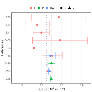
Figure 9: Values of the Sun oblateness $J_{2}^{\odot}$ obtained when considering PPN parameters $\beta$ and $\gamma$ as varying parameters. The dotted lines give the limits of the less constraining helioseismologic value from (Pijpers, 1998). F stands for Full fit, RW for random walk exploration method and P for partially fitted ephemerides (some parameters are fixed). N (respectively Y) indicates that the value has been obtained without (respectively with) LT. In y-axis, are given the references : G18 is (Genova et al., 2018), I20a (Fienga et al., 2021a), D440 (Park et al., 2017), I13c (Fienga et al., 2014), E04 and E11 in (Pitjeva and Pitjev, 2013). E00 is (Pitjeva, 2001), D405 (Standish, 2001) and I15a (Fienga et al., 2015). It is important to note that in Genova et al. (2018), only the orbit of Mercury is considered.

4.1.2 Time-scales

As mentioned in Sec. 3.2.2, planetary ephemerides produce the difference between the TT and the TDB. In the PPN framework, Eq. (86) has to be modified as follows (Manche, 2011)

$$a= -\frac{1}{2}v_{T}^{2}-\sum_{A\neq T}\frac{\mu_{A}}{r_{AT}}\,$$

$$b= -\frac{1}{8}v_{T}^{4}+\left(\beta-\frac{1}{2}\right)\left[\sum_{A\neq T}\frac{\mu_{A}}{r_{AT}}\right]^{2}+\sum_{A\neq T}\frac{\mu_{A}}{r_{AT}}\Bigg{\{}2(1+\gamma)\bm{v}_{T}.\bm{v}_{A}-(\gamma+\frac{1}{2})v_{T}^{2}$$

$$-(1+\gamma)v_{A}^{2}+\frac{1}{2}\bm{a}_{A}.\bm{r}_{AT}+\frac{1}{2}\left(\frac{\bm{v}_{A}.\bm{r}_{AT}}{r_{AT}}\right)^{2}\Bigg{\}}$$

$$+(2\beta-1)\sum_{A\neq T}\frac{\mu_{A}}{r_{AT}}\left(\sum_{B\neq A}\frac{\mu_{B}}{r_{BA}}\right).$$ (99)

Comments on reference frame theory in alternative theories

The difficult subject of reference frame systems in alternative theories has not been investigated systematically. In fact, it has been explored explicitly only for a class of massless scalar-tensor theories “à la Brans-Dicke” (Kopeikin and Vlasov, 2004), after some previous effort to characterize it in a general standard post-Newtonian approach (Klioner and Soffel, 2000). Fortunately in practice, the differences between coordinate systems in general relativity versus PPN framework are numerically negligible—notably given the already tight constraints that one already has on the PPN parameters.

4.1.3 Constraints and correlations

An important discussion related to the PPN parameter determinations using least square methods is the correlations between $\beta$, $\gamma$ and other contributions to the planetary accelerations. This problem has been pointed out a long time ago (Anderson et al., 1978) but it is still vivid today. In particular, if we consider the analytical expression of the advance of the perihelia for planetary orbits $\Delta\dot{\varpi}_{PLA}$, as given in (Will, 2014), the two main contributions of this equation are the PPN term $(2+2\gamma-\beta)$ and a term giving the impact of the Sun oblateness $J_{2}^{\odot}$. But we can also add the main belt asteroid contribution and the LT effect defined in sect. 3.3.3, such as per orbit, one gets (Bertotti et al., 2003a)

$$\Delta\dot{\varpi}_{PLA}= \mu_{\odot}(t)\times\left(\frac{2}{3}\frac{{(2\gamma-\beta+2)}}{a\,(1-e^{2})c^{2}}+\Delta\dot{\varpi}_{LT}(S,\gamma)\right)$$

$$+J_{2}^{\odot}\frac{R^{2}_{\odot}}{a^{2}\,(1-e^{2})^{2}}+\Delta\dot{\varpi}_{AST}(\mu_{AST},a_{AST},e_{AST})\,$$ (100)

where $a_{AST},e_{AST},\mu_{AST}$ are respectively the asteroid orbit semi-major axis and eccentricity and its gravitational mass perturbing the planet orbits (main-belt and trans-neptunian objects), $a,e$ are the semi-major axis and eccentricity of the planet orbit and finally, $c$ and $\mu\odot$ are the speed of light and the gravitational parameter of the Sun. This latest quantity can be time-varying as discussed in sect. 4.3.$\Delta\dot{\varpi}_{LT}(S,\gamma)$ is the Lense-Thirring effect presented in sect. 3.3.3. A discussion about other contributing terms such as PN cross-terms, de Sitter precession and 2PN crossterms has been proposed by Will (2018). The conclusion is that these 3 additional contributions could have some importances in the coming years with the Bepi-Colombo mission. In any case, they are implicitely taken into account when numerically integrating the EIHDL equation of motion.

Note that Eq. (100) is an analytical approximation of the perihelia advance rate that is useful in order to get a sense of some of the correlations that may arise between different quantities. The actual value would have to be inferred from the numerical integration of the equations of motion in the solar system with the total acceleration, $\bm{a}_{T}^{\textrm{total}}$:

$$\bm{a}_{T}^{\textrm{total}} = \bm{a}_{T}(\mu_{SS},\gamma,\beta,IC_{SS})+\bm{a}_{J_{2}^{\odot}}(\mu_{\odot},J_{2}^{\odot})+\bm{a}_{LT}(S_{\odot},\gamma),$$ (101)

where $\bm{a}_{T},\bm{a}_{J_{2}^{\odot}},\bm{a}_{LT}$ are the point-mass interaction acceleration given in Eq. (96), the acceleration induced by the oblateness of the Sun Eq. (92) and the Lense-Thirring acceleration Eq. (98) respectively, $IC_{SS}$ stands for the initial conditions of the numerical integration for the solar system bodies, including asteroids.

It is rather understandable from Eq. (100) that there can be some level of correlation between, e.g., the semi-major axis (which follows from the initial conditions in the numerical integration) and the post-Newtonian parameters $\gamma$ and $\beta$. One can also see that for disentangling the different contributions, it is more efficient to have several orbits with significantly different semi-major axis $a$ and eccentricities $e$ as the PPN acceleration depends on $a$ when the Sun oblateness acceleration depends on $a^{2}$ (see Eq. (100) and (93)). It is also interesting to compare the Sun $J_{2}^{\odot}$ determinations obtained in general relativity—equivalent to consider $\beta$ and $\gamma$ fixed to one—presented on Fig. 6 with the those obtained in adding the PPN parameters $\beta$ and $\gamma$ into the global planetary fit as on Fig 9. It appears first that, besides the differences between ephemerides, the general relativity estimations (with $\beta$ and $\gamma$ fixed to unity) have globally reduced error bars (i.e. less uncertainty induced by less correlation), as one can see, for example, with INPOP20a ($2.218\pm 0.03$ in general relativity versus $2.165\pm 0.12$ in PPN), or the partial fit obtained by Genova et al. (2018) ($2.271\pm 0.003$ in general relativity versus $2.246\pm 0.02$ in PPN). Secondly, biases affect also the $J_{2}^{\odot}$ determinations obtained with fitted PPN parameters as these latest can be significantly different from the $J_{2}^{\odot}$ values obtained in general relativity. These bias are due to the correlations between the PPN parameters and $J_{2}^{\odot}$. In the case of the Earth-Moon system, the relation is even more complex as it also includes the tidal contributions depending on the internal structures of the two bodies.

In order to overcome the problem of the correlations between the parameters, other methods of inversion such as random walk exploration or Genetic Algorithm have been proposed (see sect. 3.5). They usually give more conservative constraints than the direct least square method as it is visible on Table 5 and Fig. 8. On these Table and Figure, one can find the estimations of PPN parameters $\beta$ and $\gamma$ determinations based on planetary ephemerides. Three families of determinations are proposed. The first noted $FF$ gathers least square fitted evaluations of PPN parameters, $J_{2}^{\odot}$ and secular variation of the gravitational parameter of the Sun, $\mu_{\odot}$. As discussed previously on Sec. 3.3.4 and 3.5, these parameters are strongly correlated and thus are affected by biases (see Fig. 6 and 9) and underestimated uncertainties. The second type of determinations given on Table 5 with the label $PF$ are the one deduced with one (at least) of these parameters fixed in the planetary ephemeris adjustment. These estimations are less correlated than the $FF$ ones and give more reliable assessments but are limited to only one value (usually either $\gamma$ or $J_{2}^{\odot}$ are fixed and $\beta$ is fitted). Finally, the latest category is obtained by Genetic Algorithm (Fienga et al., 2015) or random walk exploration (Fienga et al., 2021a). They investigate the space of parameters more largely than the two former methods, leading to usually larger intervals for possible general relativity violations. On Table 5, values obtained in the context of one single planet analysis (Mercury) with only one single spacecraft (MESSENGER) data analysis (Genova et al., 2018) are also given for comparisons. The obtained results show smaller uncertainties than the planetary determinations but might be affected by possible biases. As it was shown in the Eq. (100), the use of multiple orbits favors the disentangling of the different planetary contributions. Moreover, the value of $\beta$ is obtained in introducing the Nordvedt relation Eq. (126) in the equation of motion and in the fitting procedure which supposes to consider only metric theories and increases the correlations between the fitted parameters (see sect. 4.2).

Finally, as one can see on Fig. 8, all the PPN estimations obtained with the three methods are consistent with general relativity, with no significant departure from unity for $\beta$ and $\gamma$. By considering the common overlaps of all the recently published intervals obtained with planetary ephemerides, the two following constraints are obtained:

$$(\beta-1) =(-0.45\pm 1.75)\times 10^{-5}$$

$$(\gamma-1) =(0.55\pm 1.35)\times 10^{-5}$$

These values represent an improvement of about 3 orders of magnitude for $\gamma$ and $\beta$ in comparison to the historic first determination of (Anderson et al., 1978). We can expect the same type of improvements in the coming years, especially with the outcomes of the Bepi-Colombo mission (Imperi et al., 2018; De Marchi and Cascioli, 2020).

4.1.4 The extended PPN formalism

SPN gauge versus harmonic gauge

Usually, the extended standard post-Newtonian formalism assumes a gauge (or coordinate system) that is quite different from the one recommended by the IAU that is called the standard post-Newtonian (SPN) gauge. In general relativity already, while the harmonic condition at the post-Newtonian level reads

$$g^{\alpha\beta}\Gamma^{0}_{\alpha\beta}=\mathcal{O}(c^{-5}),$$ (103)

the SPN conditions read (Damour et al., 1991)

$$\partial_{j}g_{0j}-\frac{1}{2}\partial_{0}g_{jj}=\mathcal{O}({c^{-5}}),$$ (104)

$$\partial_{j}g_{ij}-\frac{1}{2}\partial_{i}\left(g_{jj}-g_{00}\right)=\mathcal{O}(c^{-4}).$$ (105)

It implies that the field equations are modified, such that, instead of Eqs. (81-82), one has (Damour et al., 1991)

$$\Delta w^{\textrm{SPN}}=-4\pi G\sigma+\mathcal{O}(c^{-4}),$$ (106)

$$\Delta w_{i}^{\textrm{SPN}}-\frac{1}{4}\partial_{t}\partial_{i}w^{\textrm{SPN}}=-4\pi G\sigma^{i}+\mathcal{O}(c^{-2}).$$ (107)

The difference between the potentials in the harmonic and the SPN gauges reads (Soffel, 2003)

$$w^{\textrm{SPN}}=w+c^{-2}\partial^{2}_{tt}\chi/2+\mathcal{O}(c^{-3}),\qquad w_{i}^{\textrm{SPN}}=w_{i}-\partial^{2}_{ti}\chi/8,$$ (108)

with

$$\chi:=G\int d^{3}x^{\prime}\sigma\left(t,\bm{x}^{\prime}\right)\|\bm{x}-\bm{x}^{\prime}\|.$$ (109)

In terms of coordinates, the transformation between the two coordinate systems reads (Klioner and Soffel, 2000; Will, 2018b)

$${t^{\textrm{SPN}}=t-\frac{1}{2}\partial_{t}\chi},$$ (110)

$$\bm{x}^{\textrm{SPN}}=\bm{x}.$$ (111)

While both gauges can be used in principle, the harmonic gauge has been found to be much more convenient for deriving the reference frame theory in the solar system (Damour et al., 1991), such that harmonic coordinates have been used in the reference frame theory upon which the IAU recommendations have been built. A thorough comparison between the two coordinate systems in the full PPN framework can be found in (Will, 2018b).

Full PPN metric in harmonic gauge

The full PPN framework considers all the possible different potentials that could contribute to the metric, assuming that the Newtonian potential is the leading potential —which may not be the case for a massive gravity theory for instance, see sect. 4.4. Furthermore, the PPN framework can only deal with theories for which the Weak Equivalence Principle has been enforced by hand by requiring that the additional gravitational fields do not appear in the material part of the action. In the PPN framework, test particles indeed follow the geodesics of space-time, meaning that matter reacts to the space-time metric only. While this is necessary in order to have a theory for which all test particles fall alike by construction, one could question the theoretical relevance of such a restriction (Damour, 2012)—see Weak Equivalence Principle in sect. 4.2.

The full PPN metric in harmonic coordinates reads (Will, 2018b):

$$g_{00} = -1+2U+\left[2{\psi_{\text{Harm }}}-2\beta U^{2}\right]+\left(1-\frac{1}{2}\alpha_{1}+\alpha_{2}+2\xi\right)\ddot{X}+$$ (112)

$$+\Phi_{\mathrm{Harm}}^{\mathrm{PF}},$$

$$g_{0j} = -\left[2(1+\gamma)+\frac{1}{2}\alpha_{1}\right]V_{j}-\frac{1}{4}\alpha_{1}X_{,0j}+\Phi_{j\mathrm{Harm}}^{\mathrm{PF}},$$ (113)

$$g_{jk} = (1+2\gamma U)\delta_{jk}$$ (114)

with

$${\psi_{\text{Harm }}} = \frac{1}{2}(2\gamma+1-2\xi)\Phi_{1}-(2\beta-1-\xi)\Phi_{2}+\Phi_{3}+(3\gamma-2\xi)\Phi_{4}+$$ (115)

$$+\xi\Phi_{6}-\xi\Phi_{W},$$

$$\Phi_{\text{Harm }}^{\mathrm{PF}} = -\alpha_{1}w^{2}U-\alpha_{1}w^{j}V_{j}+\alpha_{2}w^{j}w^{k}X_{jk}-\left(2\alpha_{2}-\frac{1}{2}\alpha_{1}\right)w^{j}X_{,0j},$$ (116)

$$\Phi_{j\text{ Harm }}^{\mathrm{PF}} = -\frac{1}{2}\alpha_{1}w^{j}U+\frac{1}{4}\alpha_{1}w^{k}X_{jk},$$ (117)

where $\bm{w}$ is the coordinate velocity of the PPN coordinate system relative to the mean rest frame of the universe, and with the following metric potentials

$$U=\int\frac{\rho^{\prime*}}{\|\bm{x}-\bm{x}^{\prime}\|}d^{3}x^{\prime},V_{j}=\int\frac{\rho^{\prime*}v_{j}^{\prime}}{\|\bm{x}-\bm{x}^{\prime}\|}d^{3}x^{\prime},X=\int\rho^{\prime*}\|\bm{x}-\bm{x}^{\prime}\|d^{3}x^{\prime},$$ (118)

$$\Phi_{1}=\int\frac{\rho^{\prime*}v^{\prime 2}}{\|\bm{x}-\bm{x}^{\prime}\|}d^{3}x^{\prime},\quad\Phi_{6}=\int\frac{\rho^{\prime*}\left[\bm{v}^{\prime}\cdot\left(\bm{x}-\bm{x}^{\prime}\right)\right]^{2}}{\|\bm{x}-\bm{x}^{\prime}\|^{3}}d^{3}x^{\prime},$$ (119)

$$\Phi_{2}=\int\frac{\rho^{\prime*}U^{\prime}}{\|\bm{x}-\bm{x}^{\prime}\|}d^{3}x^{\prime},\quad\Phi_{3}=\int\frac{\rho^{\prime*}\Pi^{\prime}}{\|\bm{x}-\bm{x}^{\prime}\|}d^{3}x^{\prime},$$ (120)

$$\quad\Phi_{4}=\int\frac{p^{\prime}}{\|\bm{x}-\bm{x}^{\prime}\|}d^{3}x^{\prime},$$ (121)

$$\Phi_{W}=\int\rho^{*\prime}\rho^{*\prime\prime}\frac{\left(\bm{x}-\bm{x}^{\prime}\right)}{\|\bm{x}-\bm{x}^{\prime}\|^{3}}\cdot\left[\frac{\left(\bm{x}^{\prime}-\bm{x}^{\prime\prime}\right)}{\|\bm{x}-\bm{x}^{\prime\prime}\|}-\frac{\left(\bm{x}-\bm{x}^{\prime\prime}\right)}{\|\bm{x}^{\prime}-\bm{x}^{\prime\prime}\|}\right]d^{3}x^{\prime}d^{3}x^{\prime\prime},$$ (122)

where $\rho^{*}:=\rho u^{0}\sqrt{-g}$ is the “conserved” mass density—in the sense that it satisfies the Newtonian conservation equation $\partial_{t}\rho^{*}+\partial_{j}(\rho^{*}v^{j})=0$. The whole set of PPN parameters is $\gamma,\beta,\xi,\alpha_{1},\alpha_{2},\alpha_{3},\zeta_{1},\zeta_{2},\zeta_{3},\zeta_{4}$. The parameter $\xi$ is non-zero in any theory of gravity that predicts preferred-location effects such as a galaxy-induced anisotropy in the local gravitational constant GL (also called “Whitehead” effects); $\alpha_{1},\alpha_{2},\alpha_{3}$ measure whether or not the theory predicts post-Newtonian preferred-frame effects; $\alpha_{3},\zeta_{1},\zeta_{2},\zeta_{3},\zeta_{4}$ measure whether or not the theory predicts violations of global conservation laws for total momentum (Will, 2014).

Untill now, the full PPN framework has not been investigated with planetary ephemerides. First, one would have to derive the equation of motion in harmonic coordinates for point-mass interations that follows from the more general hydrodynamical situation depicted in Eqs. (112-122). Also, let us stress that the issue of the definition of the SSB has to be carefully checked, notably for the parameters that correspond to a violation of the conservation laws of momentum. Finally, the more the parameters, the more computationally demanding the study is, and one therefore has to think about the best way(s) to explore and constrain the landscape of parameters. Hence, several studies still seem to be needed before being able to constrain the full PPN framework with planetary ephemerides.

Nevertheless, measurements of PPN parameters other than $\beta$ and $\gamma$ such as $\alpha_{1},\alpha_{2},\zeta_{1}$,in the weak field regime, have been proposed early, by Anderson et al. (1978), and in the context of the mission Bepi-Colombo by Milani et al. (2002); De Marchi and Cascioli (2020), using Mercury orbit. As explained in (Will, 2014), the contribution of the preferred-frame parameters are included in the ratio between the planet mass and the Sun mass, leading to contributions to a maximum of 1$\times 10^{-4}$ for Jupiter and 1$\times 10^{-7}$ for Mercury. De Marchi and Cascioli (2020) expect a constraint for $\alpha_{1}$ at the level of $10^{-7}$ and up to 7 $\times 10^{-8}$ for $\alpha_{2}$, with Bepi-Colombo and future Venus missions. These estimations are obtained with covariance analysis of tracking observations of s/c orbiting planets. They are interesting as they estimate the capabilities of future missions for disentangling of the PPN contributions on the planetary motions.

In the strong field regime, constraints have been obtained for the parameters $\alpha_{1},\alpha_{3}$ and $\zeta_{2}$ using pulsar timing (Stairs, 2003).

4.2 Equivalence principle

While a deviation for particles with different compositions falling equally in a given gravitational field would indicate a violation of the Weak Equivalence Principle (WEP), a deviation for extended bodies with different gravitational self-energies would be a sign of a violation of the Gravitational Weak Equivalence Principle (GWEP), which is part of the Strong Equivalence Principle (SEP) as defined in (Will, 2018b). In all cases, with planetary ephemerides, one seeks to check the Universality of Free Fall (UFF)—that is, to check whether or not all bodies fall alike in a given gravitational potential. Such violations naturally occur in various modifications of general relativity, and in particular in theories with more than four dimensions like in string theories (Damour and Polyakov, 1994; Damour et al., 2002), for which the constants of the standard model of particles turn out to be dynamical entities (Damour and Donoghue, 2010; Damour, 2012).

As we will see, the violations of both the WEP and GWEP have in common the fact that the equation of motion at the Newtonian level reads as follows

$$\bm{a}_{\mathrm{T}}=-\sum_{A\neq T}\mu^{G}_{A}\frac{\bm{r}_{AT}}{r_{AT}^{3}}\left(1+\delta_{\mathrm{T}}+\delta_{AT}\right),$$ (123)

where $\delta_{T}$ and $\delta_{AT}$ are coefficients that depend on the composition of the bodies $T$ and $A$, for the case of the violation of the WEP only. For the case of the violation of the GWEP only, $\delta_{T}$ depends on the ratio between the gravitational and inertial masses and $\delta_{AT}=0$—such that

$$\left(\frac{m^{G}}{m^{I}}\right)_{T}=1+\delta_{T},$$ (124)

where $m^{G}$ and $m^{I}$ are the gravitational and inertial masses respectively. Note that $\mu^{G}_{A}$ is the gravitational parameter constructed with the gravitational mass $m^{G}_{A}$ such as $\mu^{G}_{A}=(1+\delta_{A})\mu_{A}^{I}$, where $\mu^{I}_{A}{:=Gm^{I}_{A}}$ is the gravitational parameter obtained with the inertial mass $m^{I}_{A}$. Eq. (123) is the most general equation that still satisfies Newton’s third law of motion (Viswanathan et al., 2018). As we will see in Sec. 4.6, one can have both a violation of the WEP and the GWEP at the same time—that is, $\delta_{T}$ can depend both on the composition of the body $T$ and on its internal gravitational energy.

The equivalence principle is currently tested at different scales: on the one hand on the laboratory scale for WEP with the torsion balance and MICROSCOPE, and on the other hand, the astronomical scale for GWEP with LLR and compact objects — at the level of about 10^-13 with torsion balances (Adelberger et al., 2003a), 10^-15 with the MICROSCOPE experiment (Touboul et al., 2022) and 10^-14 with LLR (Williams et al., 2012; Viswanathan et al., 2018; Biskupek et al., 2021) .

The latest LLR results (Biskupek et al., 2021) are more accurate that what can be achieved with the sensitivity of planetary ephemerides as discussed in (Viswanathan et al., 2018). We give however a brief overview of the equations at stake below, mainly in the perspective of the Bepi-Colombo mission that should lead to a significant improvement of the sensitivity of planetary ephemerides on the tests of the equivalence principle.

Finally, it is interesting to note that constraints on the violation of SEP have been obtained in strong field regime, mainly using the chronometry of millisecond pulsars. For a deeper dive into this captivating subject, we direct the reader to (Kramer et al., 2021; Freire et al., 2012; Voisin et al., 2020).

4.2.1 The case of metric theories

While metric theories satisfy the WEP by design (see Sec. 4.1) , they do not satisfy the SEP in general—in the sense that bodies with different gravitational self-energies would not follow the same trajectories in general (Nordtvedt, 1968a, b). This notably induces that for extended bodies with enough gravitational self-energy such as planets, the ratio between their gravitational and the inertial masses is no longer one as in general relativity, but instead depends on the body self-gravitational energy that can be approximated for uniformly distributed spherical bodies as follows

$$\left(\frac{m^{G}}{m^{I}}\right)^{SEP}_{T}=1+\eta\times\frac{3}{5}\frac{Gm^{G}_{T}}{c^{2}R_{T}},$$ (125)

where $R_{T}$ is the radius of the astronomical body $T$ and $m^{G}_{T}$ is its gravitational mass. The parameter $\eta$, known at the Nordtvedt parameter, quantifies the possible violation of the SEP and can be fitted together with the rest of the planetary and lunar ephemeris parameters. In the most generic case, $\eta$ can be seen as an independent parameter and be introduced in Eq. (125), common to all the bodies. However, in the case of the metric theories, it can be related to the PPN parameters such as (Will, 2018b):

$$\eta=4(\beta-1)-(\gamma-1)-\alpha_{1}-\frac{2}{3}\alpha_{2}.$$ (126)

Although note that only the cases for which $\alpha_{1}=0$ and $\alpha_{2}=0$ have been considered in planetary ephemerides so far—see Sec. 4.1.4 for a discussion on the extended parametrized post-Newtonian framework. In principle, the introduction of Eq. (126) in the global adjustment of planetary ephemerides should increase the correlations between $\beta$, $\gamma$, $\eta$ and the other ephemeris parameters, including $J_{2}^{\odot}$ (Ashby et al., 2007). However, simulations for the MORE Bepi-Colombo experiment indicate a significant improvement of the $\beta$, $J_{2}^{\odot}$ and $\eta$ correlation (from 0.9 to 0.3) thanks to the high accuracy of the Mercury-Earth range measurements that should be obtained (few tens of centimeters) by the mission (Milani et al., 2002; De Marchi et al., 2016; Imperi et al., 2018; De Marchi and Cascioli, 2020). Finally, recent attempt using Messenger tracking data leads to a measurement of $\eta$ at the level of 7 $\times 10^{-5}$ but this estimation has been done in considering only the Mercury orbit (Genova et al., 2018). Even in these very favorable conditions, it gives a slightly less restrictive limit than the latest LLR evaluation from Biskupek et al. (2021) with a deduced $\eta$ value of 5 $\times 10^{-5}$.

4.2.2 The case of non-metric theories

As discussed in Sec. 4.1, metric theories satisfy the WEP because the additional gravitational fields (beyond the metric) do not couple directly to matter. However, one could question the reason why additional gravitational fields would not couple to matter. Indeed, at the fundamental level, there does not seem to be any reason to expect that outcome (Damour, 2012). Moreover, extra-gravitational fields with non-minimal couplings to matter are ubiquitous in various attempts to unify the whole set of fundamental interactions in physics—such as in Kaluza-Klein or superstring theories (Damour, 2012), for instance. Finally, such non-minimal couplings can also appear from radiative quantum corrections of theories that satisfy the WEP at the classical level (Armendariz-Picon and Penco, 2012)—whereas the WEP in general relativity is immune to quantum corrections due to the specific symmetries of general relativity (Armendariz-Picon and Penco, 2012). Therefore, it seems that beyond general relativity, violations of the WEP should be expected at some level—either at the classical level already, or from quantum corrections to the classical action.

Decoupling mechanisms

Since the equivalence principle is observed to be satisfied with an ever increasing level of accuracy, non-metric theories need to possess mechanisms that are able to hide the effects of the additional gravitational fields in the solar system. They are often called “decoupling” or “screening” mechanisms. They can take their roots from the fact that the additional fields are simply massive enough to propagate over very short distances only—such as what happens with flux compactification in string theory (Douglas and Kachru, 2007)—or from the suppression of the coupling during the evolution of the universe—such as the Damour-Nordtvedt decoupling mechanism (Damour and Nordtvedt, 1993; Damour and Polyakov, 1994)—or from the dependence of the effective mass, or coupling, of the additional gravitational field to the local density—such as the chameleon and symmetron mechanisms (Khoury and Weltman, 2004; Hinterbichler and Khoury, 2010)—or from non-perturbative effects—such as the Vainstein mechanism (Vainshtein, 1972; Babichev and Deffayet, 2013)—or simply from exact cancellations in the field equations—such as the intrinsic decoupling (Minazzoli and Hees, 2013, 2016) that notably appears in entangled relativity (Arruga et al., 2021).

4.2.3 The equivalence principle in a planet-satellite system

Considering the generic Eq. (123), we can deduce for the couple of the bodies $T$ and $A$ that the difference between their accelerations toward the Sun $S$ reads

$$\Delta\bm{a}\equiv\bm{a}_{A}-\bm{a}_{T} = -\frac{G{\bar{m}_{AT}}}{r_{TA}^{3}}\bm{r}_{TA}+Gm^{G}_{S}\left[\frac{\bm{r}_{ST}}{r_{ST}^{3}}-\frac{\bm{r}_{SA}}{r_{SA}^{3}}\right]$$ (127)

$$+Gm^{G}_{S}\left[\frac{\bm{r}_{ST}}{r_{ST}^{3}}(\delta_{T}+\delta_{ST})-\frac{\bm{r}_{SA}}{r_{SA}^{3}}(\delta_{A}+\delta_{SA})\right],$$

with ${\bar{m}_{AT}}\equiv m^{G}_{A}+m^{G}_{T}+(\delta_{T}+\delta_{TA})m^{G}_{A}+(\delta_{A}+\delta_{TA})m^{G}_{T}$. For gravitationally bounded systems like the Earth-Moon system, one can further approximate both distances appearing in this last term as being approximately equal, such that the relevant term in order to check a potential violation of the EP through a violation of the universality of free fall (UFF) is

$$\Delta\bm{a}^{\overline{\mathrm{UFF}}}\approx\bm{a}_{\mathrm{E}}\Delta_{\mathrm{ESM}}$$ (128)

where $E$, $S$ and $M$ stand for the Earth, the Sun and the Moon respectively, and with

$$\Delta_{\mathrm{ESM}}=\left[\left(\delta_{\mathrm{E}}+\delta_{\mathrm{SE}}\right)-\left(\delta_{\mathrm{M}}+\delta_{\mathrm{SM}}\right)\right].$$ (129)

Eq. (128) was introduced in (Williams et al., 2012) for theories that violate the GWEP only, for which $\Delta_{\mathrm{ESM}}=\Delta_{\mathrm{EM}}$ such that

$$\Delta_{EM}=\left[\left(\frac{m^{G}}{m^{I}}\right)_{E}-\left(\frac{m^{G}}{m^{I}}\right)_{M}\right].$$ (130)

In that case, Eq. (128) becomes

$$\Delta\bm{a}^{\overline{\mathrm{UFF}}}\approx\bm{a}_{\mathrm{E}}\Delta_{\mathrm{EM}},$$ (131)

4.2.4 The equivalence principle at planetary scale

At planetary scale, Eqs. (128) or (131) are not valid anymore. Indeed, planets are at different distances from the Sun and EP tests cannot be limited to the differences between two accelerations. In that case, one has to use the more general Eq. (123) instead.

A confusion can occur when defining the SSB because the gravitational parameters that appear in the equations of motion are constructed with the gravitational masses; whereas the gravitational parameters that are used to define the SSB should be constructed with the inertial masses, as pointed out in Milani et al. (2002) and Genova et al. (2018)—see also Sec. 4.6. It was an issue in particular for previous versions of planetary ephemerides, such as Folkner et al. (2008), where the SSB positions and velocities were estimated at each step of integration with the gravitational parameters appearing in the equations of motion.

However, as explained in Sec. 3.2.4, in planetary ephemerides such as INPOP08 (Fienga et al., 2008) and the followings, the SSB position and velocity are estimated once, before integrating the motion of planets, using planetary initial conditions, inertial masses and Eqs. (89) and (88). As explained in Sec. 4.6, Bernus et al. (2022) have checked with a specific theory that violates both the WEP and the GWEP that those equations indeed remain the ones that characterize the SSB at the required level of accuracy for planetary ephemerides—provided that inertial masses are used for the definitions and not gravitational masses—as originally suggested in Milani et al. (2002); Genova et al. (2018).

4.2.5 Comment on the mass in the Shapiro delay equation

As soon as the SEP is violated, there is a potential ambiguity about the gravitational parameter that appears in the Shapiro delay Eq. (97). Indeed, the gravitational parameter in the Shapiro delay could either be constructed on the inertial mass, or on the gravitational mass. As we will see in Sec. 4.6 Eqs. (157-158), one can derive from first principles that the gravitational parameter that appears in the Shapiro delay is the one built upon the inertial mass, that is $\mu^{I}_{A}=Gm^{I}_{A}=(1-\delta_{A})Gm^{G}_{A}$, with :

$$c(t_{r}-t_{e}) = R+\sum_{A}(\gamma+1)\frac{\mu^{I}_{A}}{c^{2}}\ln\frac{\bm{n}\cdot\bm{r}_{rA}+r_{rA}+2\frac{(1+\gamma)\mu_{A}}{c^{2}}}{\bm{n}\cdot\bm{r}_{eA}+r_{eA}+2\frac{(1+\gamma)\mu_{A}}{c^{2}}}\,,$$ (132)

$$= R+\sum_{A}(\gamma+1)\frac{\mu^{G}_{A}}{c^{2}}\left(1-\eta\times\frac{3}{5}\frac{\mu^{G}_{A}}{c^{2}R_{A}}\right)\times$$

$$\qquad\qquad\ln\frac{\bm{n}\cdot\bm{r}_{rA}+r_{rA}+2\frac{(1+\gamma)\mu_{A}}{c^{2}}}{\bm{n}\cdot\bm{r}_{eA}+r_{eA}+2\frac{(1+\gamma)\mu_{A}}{c^{2}}}\,.$$

There is a somewhat simple explanation to that. One must recall that the original Nordtvedt effect was derived for the sum of point particles of (inertial) mass $m$ that are gravitationally bounded together. The metric is bent by those masses $m$, and the sum of all the masses correponds to the inertial mass of the overall body that is composed from all thoses masses, to lowest order (Nordtvedt, 1968b). Since the Shapido delay simply derives from the null condition $ds^{2}=0$ for light, the Shapiro delay must depend on this sum of inertial masses. What the Nordtvedt effect tells additionally, is that the center of mass of this collection of masses does not follow the same trajectory as would an inertial mass, but follows the trajectory given by the following equation instead

$$\bm{a}_{\mathrm{T}}=-\sum_{A\neq T}\mu^{G}_{A}\frac{\bm{r}_{AT}}{r_{AT}^{3}}\left(1+\eta\times\frac{3}{5}\frac{\mu^{G}_{T}}{c^{2}R_{T}}\right).$$ (134)

4.2.6 The issue of time in non-metric theories

The issue with theories that violate the WEP is that they usually also violate the local position invariance (Uzan, 2011), such that the behaviour of clocks not only may be modified with respect to general relativity depending on the position in the gravitational field, but also may depend on the clock composition. Therefore, one may expect that this should complicate the tests of such theories with planetary ephemerides, given that positions of astronomical bodies are given in one of the coordinate times recommended by the IAU, and which are perfectly independent of the composition of the clocks that has been used. Fortunately, the local position invariance is tested to a very high level of accuracy on Earth with various atomic clocks (Rosenband et al., 2008; Guéna et al., 2012; Leefer et al., 2013; Godun et al., 2014; Huntemann et al., 2014). Indeed, thanks to the eccentricity of the Earth’s orbit, one can probe a potential variation of the ratio between the frequencies of atomic clock with different compositions depending on the variation of the local value of the Sun’s gravitational field. Because the local position invariance is tested with atomic clocks at a level of accuracy that is far beyond what is used in space navigation, one can neglect this potential effect in planetary ephemerides.

4.3 Variation of the gravitational constant G

With respect to the subject of the potential variation of constants (Uzan, 2011), planetary and lunar ephemerides have been mostly used for testing an hypothetical variation of Newton’s constant $G$, or a related value, the Astronomical Unit (Hellings et al., 1983; Anderson et al., 1987, 1989; Pitjeva, 1993).

Before 2012 and the decision by the International Astronomical Union (Capitaine et al., 2012) to redefine the Astronomical Unit (AU) as a constant with a fixed value, the AU was indeed part of the parameters estimated during the construction of planetary ephemerides. The Gauss constant $k$ was fixed (Standish, 2001) and the AU was estimated from this equation

$$GM_{\odot}=(AU)^{3}k^{2}/D^{2}$$ (135)

where D is the length of the day and $GM_{\odot}$ is the gravitational parameter of the Sun. In this context, AU values and its hypothetical time variations have been estimated with planetary fit by Krasinsky and Brumberg (2004). In the same manner, an estimation of $\frac{\dot{G}}{G}$ was also obtained, together with the value of AU. A first test of such a variation has been initiated by Hellings et al. (1983), using the data obtained with the Viking mission on Mars. On a regular basis, the planetary ephemerides were then published with updates for $\frac{\dot{G}}{G}$ based on a global adjustment including also AU and PPN parameters (Pitjeva, 1993; Standish, 2001; Pitjeva, 2005b). Results are gathered in Table 6.

After 2012, the AU has been fixed to 149597870700 m, closing the door to the estimation of $d{AU}/dt$, but leading to a more consistent determination of the gravitational parameter of the Sun, $GM_{\odot}$ noted $\mu_{\odot}$, now fitted in planetary ephemerides. As it is reviewed in Uzan (2011), some theories propose that the gravitational constant can vary with time. Thus, an hypothetical variation of $G$ in time has been introduced in the planetary ephemerides, but it is not straightforward since it affects both the planetary and the Sun gravitational parameters $\mu$. .

For the planets, because they do not lose or gain mass, the time variation of G induces a direct variation of the gravitational parameter $\mu_{P}$ such $\dot{\mu}_{P}/\mu_{P}=\dot{G}/G$. For the Sun, its intrinsic mass loss $\dot{M_{\odot}}$ has also to be considered. As a consequence, the following equations are added to the system of equations integrated numerically during the planetary ephemerides construction

$$\frac{\dot{\mu}_{\odot}}{\mu_{\odot}} = \frac{\dot{G}}{G}+\frac{\dot{M_{\odot}}}{M_{\odot}},$$ (136)

where ${\mu}_{\odot}$ is the gravitational paramater of the Sun and

$$\frac{\dot{\mu}_{P}}{\mu_{P}} = \frac{\dot{G}}{G},$$ (137)

with $\mu_{P}$ is the gravitational parameter of bodies other than the Sun.

At each step $t$ of the numerical integration of the planetary equations of motion, the following quantities are estimated :

$$M_{\odot}(t)=M_{\odot}(t_{0})+(t-t_{0})\times\dot{M_{\odot}},$$ (138)

$$M_{P}(t)=M_{P},$$ (139)

$$G(t)=G(t_{0})+(t-t_{0})\times\dot{G},$$ (140)

$$\mu(t)=G(t)\times M(t),$$ (141)

where $t_{0}$ is the date of the origin of the planetary ephemeris. Let us note that the gravitational parameter $\mu(t)$ also appears in the computation of the Shapiro delay (see sect 3.4.1). In this case, the value of $\mu(t)$, corresponding to the date of the observation, is computed with Eq. (141) and re-introduced in the Shapiro Eq. (94).

$M_{\odot}(t_{0})$ is the mass of the Sun fitted during the construction of the ephemeris, and $G(t_{0})$ is the Newtonian gravitation constant as defined by the IAU (Luzum et al., 2011). The effect of the time variation of G being largely induced by the gravitational parameter of the Sun more that the ones of the planets, one then deduces the value of $\dot{G}/G$ by considering its impact of the Sun contribution (Eq. 136) and a fixed value for the Sun total mass loss, $\frac{\dot{M_{\odot}}}{M_{\odot}}$. Pitjeva and Pitjev (2012) have proposed an interval of values for the total solar mass loss of

$$\frac{\dot{M_{\odot}}}{M_{\odot}}=(-0.67\pm 0.31)\times 10^{-13}{{\quad(2\sigma)}}\,\textrm{yr}^{-1},$$ (142)

This estimation considers the mass loss by the Sun, but also the mass gained by falling materials (comets, asteroids etc…). Pinto et al. (2011) have estimated a mean mass loss from wind emission of charged particles during the 11-year solar cycle :

$$\frac{\dot{M_{\odot}}}{M_{\odot}}=(-0.55\pm 0.15)\times 10^{-13}\,{{\quad(3\sigma)}}\,\textrm{yr}^{-1},$$ (143)

instead of Eq. (142). In 2021, a detailed evaluation of Pitjeva et al. (2021) gives

$$\frac{\dot{M_{\odot}}}{M_{\odot}}={{(-1.105\pm 0.235)\times 10^{-13}\quad(3\sigma)}}\,\textrm{yr}^{-1},$$ (144)

This value accounts for the solar wind radiation as well as the accumulation of interplanetary dust falling on the Sun together with comets. The authors conclude that the value of $\frac{\dot{M_{\odot}}}{M_{\odot}}$ in Pitjeva and Pitjev (2012) is overestimated

On Table 6, are gathered the values of $\dot{\mu_{\odot}}/{\mu\odot}$ obtained by different authors jointly with PPN parameter estimations as well as the $\dot{G}/G$ deduced using the value of $\frac{\dot{M_{\odot}}}{M_{\odot}}$ specified in the same Table. It is important to stress that the correlations between the PPN parameters, $\dot{\mu_{\odot}}/{\mu_{\odot}}$ and the other fitted parameters of the planetary ephemerides being non zero (see i.e. Table 6 from Fienga et al. (2015)), the values given in Table 6 have to be considered as part of a global fit, and consequently they are planetary ephemeris dependent. Direct adjustments with all parameters fitted together (Pitjeva and Pitjev, 2013; Pitjeva et al., 2021), partial fits (Konopliv et al., 2011; Fienga et al., 2021a) but also random walk exploration algorithms have been used for obtaining constraints on $\dot{\mu_{\odot}}/{\mu_{\odot}}$, given in Table 6. As explained in Sect 3.5 and 4.1, the partial fit consists to fix one PPN parameter and then fit $\dot{\mu_{\odot}}/{\mu_{\odot}}$ together with the rest of the planetary parameters. The random walk exploration algorithm fixes the PPN parameters and $\dot{\mu_{\odot}}/{\mu_{\odot}}$ according to random values, and performs a regular fit for the rest of the planetary parameters. The obtained ephemerides are then selected according to different statistical criteria (Fienga et al., 2015, 2021a). The latest two approaches (partial fit and random walk exploration algorithms) give larger intervals of possible values than the direct fit of all parameters, as one can see in Table 6.

One can also mention $\dot{G}/G$ estimations deduced, not directly from planetary ephemerides, but from the adjustment of one single planet orbit during the analysis of radar tracking data analysis of one given space mission. This is the case for example with Mercury and the MESSENGER data operated by Genova et al. (2018), noted MSG in Table 6. In this work, it has to be stressed that only Mercury orbit was considered in the analysis. Nevertheless, in all the cases produced in Table 6, no clear indication of a time variation of G is visible, despite the improvements of the planetary ephemerides and of the estimation of the solar mass loss (Pitjeva et al., 2021). Finally, other technics or methods have been used for measuring possible variations of the gravitational constant, G. One can cite for example, the determination of $\dot{G}/G$ deduced from pulsar timing (Stairs, 2003; Zhu et al., 2015, 2018; Kramer et al., 2021). The obtained limit is then one order of magnitude greater (i.e. $\lvert\dot{G}/G\rvert<0.9\times 10^{-12}$ yr^-1 from Zhu et al. (2018)) than the one obtained with planetary ephemerides although the gravitational regimes are quite different (strong field regime for the pulsar measurements and weak field for planetary ephemerides).

Table 6: Values of $\dot{\mu_{\odot}}/{\mu_{\odot}}$ found in the literature deduced from planetary ephemerides. The Column 3 indicates the type of method used for the estimation: either the full fit (FF), the partial fit (PF) in or the random walk exploration (RW). See text for details. For Fienga et al. (2021a), PF^∗∗ indicates that the oblateness of the Sun is strongly constrained by helio-seismological value. So this solution cannot be seen as a free fit but as a partial fit. Analysis of the MESSENGER mission is labeled MSG in Column 3 using only the Mercury orbit. The $\dot{G}/G$ values are deduced with $\dot{\mu}/{\mu}$ and ${\dot{M_{\odot}}}/{M_{\odot}}$ given in Column 5. The value of $\dot{G}/G$ deduced from Pitjeva and Pitjev (2013) is not the one published by the authors but was obtained in using the same value of ${\dot{M_{\odot}}}/{M_{\odot}}$ as for Konopliv et al. (2011).

Reference	PE	Method	$\dot{\mu_{\odot}}/{\mu_{\odot}}$	$\frac{\dot{M_{\odot}}}{M_{\odot}}$	$\dot{G}/G$
			$\times$ 1014 yr-1	$\times$ 1014 yr-1	$\times$ 1014 yr-1
Before AU fixed
Pitjeva (1993)	EPM1988	FF	NA	NA	470 $\pm$ 470
Pitjeva (2001)	EPM2000	FF	NA	NA	4 $\pm$ 8
Standish (2001)	DE405	FF	NA	NA	1 $\pm$ 8
Pitjeva (2005b)	EPM2004	FF	NA	NA	-2 $\pm$ 5
After AU fixed
Konopliv et al. (2011)	DE421	PF	1 $\pm$ 16	-9.2 $\pm$ 6.1	10.2 $\pm$ 22.1∗
Pitjeva and Pitjev (2012)	EPM2010	FF	-5 $\pm$ 4	-6.7 $\pm$ 3.1	1.65 $\pm$ 8.77
Pitjeva and Pitjev (2013)	EPM2011	FF	-6.3 $\pm$ 6.4	-6.7 $\pm$ 3.1	0.4 $\pm$ 11.1
Fienga et al. (2015)	INPOP15a	FF	-5.0 $\pm$ 2.9	-9.2 $\pm$ 6.1	4.2 $\pm$ 9.0
		RW	-4.3 $\pm$ 7.4	-9.2 $\pm$ 6.1	4.9 $\pm$ 13.5
Genova et al. (2018)		MSG	-6.130 $\pm$ 1.47	-10 $\pm$ 1	4 $\pm$ 7.5
Pitjeva et al. (2021)	EPM2021	FF	-10.2 $\pm$ 1.4	-11.05 $\pm$ 2.35	0.85 $\pm$ 3.75
Fienga et al. (2021a)	INPOP20a	PF∗∗	-8.8 $\pm$ 2.9	-9.2 $\pm$ 6.1	0.4 $\pm$ 9.0
				-11.05 $\pm$ 2.35	2.25 $\pm$ 5.25
		RW	-10.3 $\pm$ 22.8	-9.2 $\pm$ 6.1	-0.8 $\pm$ 28.4

4.4 Massive gravity

Unlike in electromagnetism—- like with the Procca theory (de Rham, 2014; Proca, 1936)—-, there is not a unique definition for what massive gravity might entail (de Rham, 2014). In field theory, massive interactions typically result in a Yukawa suppression of these interactions at the scale of the Compton wavelength. However, due to its tensorial rather than vectorial nature, this may not necessarily be the case for a fully consistent theory of massive gravity (de Rham, 2014). Nonetheless, from a phenomenological perspective, it is possible to test whether a Yukawa suppression of gravitational potentials occurs within the solar system. Formally, this would lead to the following modification of the Newtonian potential (Will, 2018a)

$$w=w_{\textrm{Newton}}\mathrm{exp}(-r/\lambda_{g}),$$ (145)

which can be developped as Bernus et al. (2019)

$$w=w_{\textrm{Newton}}\left(1+\frac{1}{2}\frac{r^{2}}{\lambda_{g}^{2}}\right)+\mathcal{O}{(\lambda_{g}^{-3})},$$ (146)

after a convenient change of coordinate system that absorbs the constant term in the gravitational potential—which has no impact on the observables.

As discussed in Sect 4.5, this modification is different from a fifth force, for which the new potential is an affine function of the Yukawa suppression instead of a linear function (Fischbach et al., 1992; Will, 2014). Fifth forces usually originate from the existence of an additional gravitational field that is massive—e.g. a massive scalar field (Wagoner, 1970; Hees et al., 2018)—rather than considering that the field equation on the metric perturbation itself has a mass term. Indeed, Eq. (145) is solution of a massive gravitational potential equation that reads

$$\Delta w-\frac{w}{\lambda_{g}^{2}}=-4\pi G\sigma.$$ (147)

Obviously, as long as $\lambda_{g}$ is big enough, the gravitational phenomenology in the Newtonian regime can reduce to the one of general relativity to any given level of accuracy. Also, if $\lambda_{g}$ is large enough that only the leading order correction in Eq. (146) has a significant contribution to the metric, one can assume that only the Newtonian part of the post-Newtonian expansion is modified with respect to the equations of motion in general relativity Eq. (90).
In that situation, the equation of motion only has one extra term with respect to the usual EIHDL equation Eq. (96) that reads Bernus et al. (2019)

$$\delta\bm{a}_{A}^{\lambda_{g}}=\frac{1}{2\lambda_{g}^{2}}\sum_{A\neq T}\frac{\mu_{T}}{r_{AT}}\bm{r}_{AT}+\mathcal{O}(\lambda_{g}^{-3}),$$ (148)

and further assuming that light still propagates along null geodesics, the Shapiro delay reads (Bernus et al., 2019)

$$c(t_{r}-t_{e}) = c(t_{r}-t_{e})_{GRT}$$

$$+\sum_{A}\frac{\mu_{A}}{c^{2}}\frac{1}{2\lambda_{g}^{2}}\ln\left[b^{2}\frac{\bm{n}\cdot\bm{r}_{rA}+r_{rA}}{\bm{n}\cdot\bm{r}_{eA}+r_{eA}}+\bm{n}\cdot(r_{rA}\bm{r}_{rA}-r_{eA}\bm{r}_{eA})\right]\,,$$

where $c(t_{r}-t_{e})_{GRT}$ corresponds to the general relativity light time given in Eq. (94), $b$ is the minimal distance between the light path and the central body (here the Sun). This expression is an approximation at c^-2 level, the additional terms induced by gravitational field mass being negligible relative to the present day accuracy for commonly admitted $\lambda_{g}$ (with $\lambda_{g}>2.8\times 10^{12}$ km (Will, 2018a, 1998)).

Likewise, from Eq. (146), the difference between a clock $A$ and a BCRS time $t$ still is

$$\frac{d\tau_{A}}{dt}=1-\frac{1}{c^{2}}\left[v_{A}^{2}/2+U\left(\mathbf{x}_{A}\right)\right],$$ (150)

up to terms of order $\mathcal{O}{(\lambda_{g}^{-2}c^{-2})}$. For instance, assuming a conservative bound of $\lambda_{g}>2\times 10^{12}$ km, the correction to Eq. (150) at the surface of the Earth would be less than $10^{-17}(\sim R_{\oplus}^{2}/\lambda_{g}^{2}\textrm{, where }R_{\oplus}\textrm{ is the radius of the Earth})$ time less than the contribution of the last term in the bracket of Eq. (150)—that is, far beyond what can be achieved with present clocks stability (Guena et al., 2012).

By analogy with standard quantum physics, the Compton length can also be interpreted in terms of a mass of the graviton $m_{g}$ following the relation:

$$\lambda_{g}=\frac{\hbar}{cm_{g}},$$ (151)

with $\hbar$ the Planck constant, and $c$ the speed of light. In 2018, Will (2018a) proposed to use solar system ephemerides to improve the constraints on $\lambda_{g}$ in the Newtonian limit. The starting point was that a massive gravitational field should lead to a modification of the perihelion advance of solar system bodies. Hence, based on current constraints on the perihelion advance of Mars derived from Mars Reconnaissance Orbiter (MRO) data, Will estimates that the Compton wavelength should be bigger than $(1.4-2.7)\times 10^{14}$km (resp. $m_{g}<(4-8)\times 10^{-24}$ eV/$c^{2}$), depending on the specific analysis. However, making an estimation from quantities derived from ephemerides that assumed other theorerical frameworks—here, the perihela advances per orbit and their uncertainty in either general relativity or PPN frameworks—cannot account for the fact that the mass of the graviton is correlated to the various parameters of the ephemeris (eg. masses, semi-major axes etc.). While a graviton with a non-zero mass may impact the solar system dynamics, so also does a change of the various other parameters of the ephemerides. Because of the correlation between $m_{g}$ (or $\lambda_{g}$) and other parameters, any modification induced by a non-null value of $m_{g}$ may—at least in part—be reabsorbed by the modification of other parameters of the ephemerides.

In order to overcome this issue, Bernus et al. (2019, 2020) and Mariani et al. (2023) have built planetary ephemerides fully developed in the massive gravity framework of Eq. (145) and fitted over the data sample of INPOP17a , INPOP19a and INPOP21a respectively. The results of these investigations are given on Table 7.

Bernus et al. (2019, 2020) had used a method of random walk exploration that is more conservative that the Monte Carlo Markov Chain (MCMC) algorithm used by Mariani et al. (2023). With the same random walk exploration method, but using the updated INPOP21a ephemerides, Mariani et al. (2023) obtained a constraint that is 3 times smaller than Bernus et al. (2020). This improvement is induced by the use in INPOP21a of the latest Juno and Mars orbiter tracking data up to 2020 as well as a fit of the Moon-Earth system to LLR observations also up to 2020. By improving the procedure with MCMC, Mariani et al. (2023) was able to push the limit of detection of the mass of the graviton at a new level, with a constraint at $1.01\times 10^{-24}\;eVc^{-2}$ (resp. $\lambda_{g}\geq 122.48\times 10^{13}\;km$) with a $99.7\%$ confidence level.

It is somewhat interesting to compare these constraints to the ones deduced from the observation of gravitational waves. Indeed, it is assumed that a massive gravitational field that leads to Eq. (147) might also modify the dispersion relation of gravitational waves as follows (Abbott et al., 2021; Will, 1998)

$$E^{2}=p^{2}c^{2}+m_{g}c^{2},$$ (152)

where $E$ and $p$ are the energy and momentum of the wave.

Such a modified dispersion relation causes gravitational waves frequency modes to propagate at different speeds, leading to an overall modification of the phase morphology of gravitational waves with respect to the general relativity predictions. Since the morphology of gravitational wave phase has been consistent with general relativity so far, it led to severe constraints on the value of $m_{g}$ that are reproduced on Table 7.

Even if a massive gravity theory actually leads to both the phenomenological consequences represented in Eqs. (147) and (152), there is absolutely no reason for the constraints from ephemerides on the one hand, and from gravitational waves on the other hand, to be at the same level accuracy.

Each type of constraints is relevant on its own right given that they test different phenomenologies—that is, Eq. (145) versus Eq. (152)—which may (or may not) be related, depending on the underlying massive gravity theory that one is considering. For instance, screening mechanisms that kick-in for high density environments—such as the Vainshtein mechanism (Babichev and Deffayet, 2013)—may impact Eq. (145) and not Eq. (152). This notably seems to be the case for ghost-free massive gravity (de Rham, 2014).

Table 7: Limits obtained for the Compton length $\lambda_{g}$ in km as defined in Eqs. (148) and (4.4). Are also given the corresponding values in term graviton mass $m_{g}$ in eV$/c^{2}$. Are also indicated, for comparisons, the values obtained with INPOP17a (Bernus et al., 2019), INPOP19a (Bernus et al., 2020), and INPOP21a (Mariani et al., 2023) as well as the estimations for the dynamical mode from Virgo-Ligo GWTC-1 and GWTC-3 (Abbott et al., 2019, 2021). For INPOP21a, two values at 90$\%$ confidence level (CL) are given : the one indicated in the column RW corresponds to value obtained with the same method (random walk exploration) as Bernus et al. (2019) and Bernus et al. (2020) and the one given in Column MC corresponds to MCMC results.

	GWTC-1	GWTC-3	INPOP17a	INPOP19a	INPOP21a
					RW	MCMC
CL	0.90	0.90	0.90	0.90	0.9	0.9
Graviton mass
$\lambda_{g}\times 10^{-13}$ [km]	2.6	9.77	1.83	3.93	12.01	209.67
$m_{g}\times 10^{23}$ [eV/c2]	4.7	1.27	6.76	3.16	1.03	0.059
Fifth Force
$\frac{\lambda}{\sqrt{\mid\alpha\mid}}\times 10^{-13}$[km], $\alpha>0$			1.83	3.93
$\frac{\lambda}{\sqrt{\mid\alpha\mid}}\times 10^{-13}$[km], $\alpha<0$				3.77

4.5 Yukawa potential and Fifth Force

Whereas one can imagine that the metric field itself has a mass—see Sec. 4.4—it is also possible to imagine the existence of additional gravitational fields that are massive, while the metric field would remain massless. In such situations, the potential often becomes an affine function of the Yukawa suppression as follows (Wagoner, 1970; Fischbach et al., 1992; Will, 2014)

$$w=w_{\textrm{Newton}}(1+\alpha\mathrm{exp}(-r/\lambda)),$$ (153)

where $\alpha$ is the strength (relative to gravity) and $\lambda$ the range of the force. This type of modifications of the Newtonian potential is often referred to as a fifth force (Will, 2014).
Depending on whether the additional massive field couples universally to matter or not, the fifth force can be either composition-dependent or independent (Will, 2014). Solar system tests—such as the ones realised with planetary ephemerides—usually focus on composition independent models. In Konopliv et al. (2011), constraints on the Yukawa potential were deduced from the analysis of Mars orbiter tracking data and from the construction of a Mars updated ephemeris. Fig. 10 shows that already in 2011, the constraints from planetary ephemerides were at the level of the constraints from lunar ephemerides. As explained in Bernus et al. (2019), in the limit $\lambda\gg r$ and with $\alpha>0$, one can use the constraints given in Sect 4.4 for the test of massive graviton, in order to deduce constraints on the Yukawa potential. These constraints are given in Table 7 and Fig. 10. The green lines on this Figure show the improvements of the new generation of planetary ephemerides relative to the one use in Konopliv et al. (2011), as well as the new limits obtained at solar system scale. A new limit (labelled IBC) obtained by simulating the introduction of Bepi-Colombo MORE experiments as predicted by De Marchi and Cascioli (2020) and Fienga et al. (2022) is also indicated. Let note that, because fifth force models in Eq. (153) depend on two parameters ($\alpha$ and $\lambda$), whereas the massive graviton models in Eq. (145) depend on only one ($\lambda_{g}$), the mapping between the two breaks down for small Compton wavelength. This explains why the green lines in Fig. 10 are restricted to the right part of the plot.

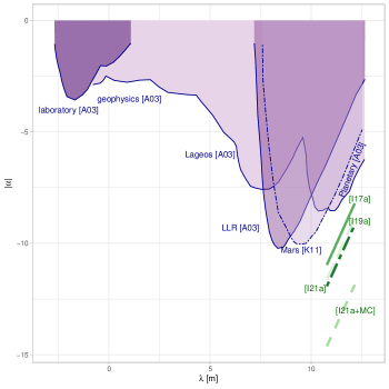
Figure 10: Observational constraints obtained for the Yukawa potential extracted from A03, standing for Adelberger et al. (2003b). The green lines give the constraints deduced from the INPOP planetary ephemerides graviton tests presented in Table 7 : I17a stands for Bernus et al. (2019), I19a for Bernus et al. (2020), I21a and I21a+MC for Mariani et al. (2023). K11 indicates the limits deduced from Mars tracking data analysis by Konopliv et al. (2011).

4.6 Einstein-dilaton theories

The case of Einstein-dilaton theories is somewhat very interesting for the phenomology of alternative theories in the solar system, because it allows one to consistently derive the equations of motion, Shapiro delay and conserved quantities in a framework that leads to a violation of both the WEP and the GWEP.

Einstein-dilaton theories are scalar-tensor theories that violate the WEP at the fundamental level, because they possess at least one massless scalar-field that couples non-minimally to matter fields. They are somewhat expected as being the low energy effective gravitational action of string theories (Damour and Polyakov, 1994; Damour et al., 2002)—and other higher than four dimensional theories (Overduin and Wesson, 1997)—which generically predict the existence of one (or several) additional scalar-field(s) that mediates gravity: the dilaton field (and the moduli fields that come from the compactification of the extra-dimensions in string theories). Tests of Einstein-dilaton theories with planetary motions have been proposed by Damour and Donoghue (2011) based on the equations of Damour and Donoghue (2010). The first results for the massless dilaton with planetary ephemerides have been published in Bernus et al. (2022).

4.6.1 Equations of motion and Shapiro delay

The general action for an Einstein-dilaton theory may be written as (Minazzoli and Hees, 2016; Bernus et al., 2022)

$$S\left[\bm{g},\psi_{i},\varphi\right]= \frac{1}{2\kappa c}\int\left(f(\varphi)R-\frac{\omega(\varphi)}{\varphi}\varphi^{\mu}\varphi_{,\mu}\right)\sqrt{-g}\mathrm{~{}d}^{4}x$$ (154)

$$+\frac{1}{c}\int\left(\mathcal{L}_{\mathrm{SM}}\left[\bm{g},\psi_{i}\right]+\mathcal{L}_{\mathrm{int}}\left[\bm{g},\psi_{i},\varphi\right]\right)\sqrt{-g}\mathrm{~{}d}^{4}x$$

where $\mathcal{L}_{\mathrm{SM}}$ is the Lagrangian density of matter described by the standard model of particle physics and $\mathcal{L}_{\mathrm{int}}$ the Lagrangian density of the interactions between the dilaton field $\varphi$ and matter. Such interactions can be parametrized by arbitrary functions of the scalar-field as follows

$$\mathcal{L}_{int} =-\frac{D_{e}(\varphi)\beta_{e}(e)}{2e}F_{\mu\nu}F^{\mu\nu}-\frac{D_{g}(\varphi)\beta_{3}(g_{3})}{2g_{3}}G^{a}_{\mu\nu}G_{a}^{\mu\nu}$$

$$-\sum_{i=e,u,d}(D_{m_{i}}(\varphi)+\gamma_{m_{i}}D_{g}(\varphi))m_{i}\bar{\psi}_{i}\psi_{i}$$ (155)

where $F_{\mu\nu}$ is the Faraday tensor, $G^{a}_{\mu\nu}$ is the gluons tensor, $e$ and $g_{3}$ are respectively the photons and the gluons coupling constants, $\beta_{e}(e)=\lambda\partial\ln e/\partial\lambda$ and $\beta_{3}(g_{3})=\lambda\partial\ln g_{3}/\partial\lambda$ are their respective beta functions relative to the quantum scale invariance violation, where $\lambda$ is the energy scale of the considered physical processes, $m_{i}$ is the fermion mass, $\psi_{i}$ their spinor, and $\gamma_{m_{i}}=-\lambda\partial\ln m/\partial\lambda$ is the beta function relative to the dimensional anomaly of the fermion masses coupled to the gluons. The $D_{i}(\varphi)$ functions describe the different couplings between the matter fields and the dilaton. This Lagrangian density is a straightforward non-linear generalisation of the action considered by Damour and Donoghue (2010).

Assuming a linear coupling—such as in Damour and Donoghue (2010)—and at leading order in the composition dependent effects, the acceleration reads (Bernus et al., 2022)

$$\bm{a}_{T}= -\sum_{A\neq T}\frac{\mu_{A}}{r_{AT}^{3}}\bm{r}_{AT}\left(1+\delta_{T}+\delta_{AT}\right)-\sum_{A\neq T}\frac{\mu_{A}}{r_{AT}^{3}c^{2}}\bm{r}_{AT}\Bigg{\{}\gamma v_{T}^{2}+(\gamma+1)v_{A}^{2}$$

$$-2(1+\gamma)\bm{v}_{A}.\bm{v}_{T}-\frac{3}{2}\left(\frac{\bm{r}_{AT}.\bm{v}_{A}}{r_{AT}}\right)^{2}-\frac{1}{2}\bm{r}_{AT}.\bm{a}_{A}-2\gamma\sum_{B\neq T}\frac{\mu_{B}}{r_{TB}}+\sum_{B\neq A}\frac{\mu_{B}}{r_{AB}}\Bigg{\}}$$

$$+\sum_{A\neq T}\frac{\mu_{A}}{c^{2}r_{AT}^{3}}\left[2(1+\gamma)\bm{r}_{AT}.\bm{v}_{T}-(1+2\gamma)\bm{r}_{AT}.\bm{v}_{A}\right](\bm{v}_{T}-\bm{v}_{A})$$

$$+\frac{3+4\gamma}{2}\sum_{A\neq T}\frac{\mu_{A}}{c^{2}r_{AT}}\bm{a}_{A}$$ (156)

Eq. (156) depends on $\gamma=(1-\alpha_{0}^{2})/(1+\alpha_{0}^{2})$ and $\delta_{A}=\delta_{A}^{d}+\delta_{A}^{N}$ with $\delta_{A}^{d}=\alpha_{0}\tilde{\alpha}_{A}/(1+\alpha_{0}^{2})$ and $\delta_{A}^{N}=(\gamma-1)\omega_{A}\mid/\tilde{m}_{A}c^{2}$ where $\omega_{A}$ is the self-gravitational energy of the body A. The fundamental parameters on top of which they are built are $\alpha_{0}$, the universal coupling constant, and $\tilde{\alpha}_{A}=d_{\hat{m}}Q_{\hat{m}}^{A}+d_{\delta m}Q_{\delta m}^{A}+d_{m_{e}}Q_{m_{e}}^{A}+d_{e}Q_{e}^{A}$, where $Q_{\hat{m}}^{A}$, $Q_{\delta m}^{A}$, $Q_{m_{e}}^{A}$, and $Q_{e}^{A}$ are the dilatonic charges, estimated according to the composition of the considered bodies. In these equations, $A$ stands for the planet to consider, $\mu_{A}$ being its gravitational parameter. Bernus et al. (2022) simplify the problem by considering two average charges for the telluric and gaseous bodies only, because of the similar dilatonic charges for these two classes of objects. This approximation leads to the reduction of the number of the tested parameters from 10 to 3 for the linear coupling case: $\alpha_{0}$, $\tilde{\alpha}_{T}$, $\tilde{\alpha}_{G}$, for which $T$ and $G$ stand for telluric and gaseous bodies respectively. Let note that $\mu_{A}$ is here the product of $G$ with the gravitational mass $m^{G}_{A}$.
From there, one has to also account for different effects, such as the Nordvedt effect that (in the case of the linear coupling) reads $\delta_{A}^{N}=-(1-\gamma)\frac{3\mu_{A}}{5R_{A}c^{2}}$ with $R_{A}$ the planet radius, or the modification of the time travel that, at the required level of accuracy, reads (Bernus et al., 2022)

$${c(t_{r}-t_{e})=R+\sum_{A}(1+\gamma-\delta_{A})\frac{\mu_{A}}{c^{2}}\ln\frac{\bm{n}\cdot\bm{r}_{rA}+r_{rA}+\frac{4\mu_{A}}{c^{2}}}{\bm{n}\cdot\bm{r}_{eA}+r_{eA}+\frac{4\mu_{A}}{c^{2}}}\,.}$$ (157)

Let us note that

$$(1+\gamma-\delta_{A})\mu_{A}=(1+\gamma)\mu^{I}_{A},$$ (158)

at the required level of accuracy, where $\mu_{A}^{I}$ is the gravitational parameter constructed with the inertial mass, such that $\mu^{I}_{A}=(1-\delta_{A})\mu_{A}$. This means that the mass involved in the Shapiro delay is the inertial mass and not the gravitational mass—as already discussed in Sec. 4.2.5.

4.6.2 Conserved quantities and the definition of the SSB

From the Lagrangian formulation of the equations of motion, Bernus et al. (2022) show that the following barycenter constant vector is a first integral of the equations of motion

$$\bm{q}=\bm{G}-\bm{V}t,$$ (159)

where

$$\bm{G}=\frac{c^{2}}{h}\sum_{A}\mu_{A}\bm{z}_{A}\left(1-\delta_{A}+\frac{v_{A}^{2}}{2c^{2}}-\frac{1}{2c^{2}}\sum_{B\neq A}\frac{\mu_{B}}{r_{AB}}\right)$$ (160)

are the coordinates of the relativistic barycenter of the system and

$$\bm{V}=\frac{c^{2}\bm{P}}{h}$$ (161)

is the velocity of the barycenter motion. $h$ is the conserved energy—whose value does not affect what follows but can be found in Bernus et al. (2022)—and $\bm{P}$ is the conserved linear momentum that reads

$$\bm{P} =\sum_{A}\bm{p}_{A}$$

$$=\sum_{A}\mu_{A}\bm{v}_{A}\left[1-\delta_{A}+\frac{1}{2c^{2}}\left(v_{A}^{2}-\sum_{B\neq A}\frac{\mu_{B}}{r_{AB}}\right)\right]$$

$$\quad-\frac{1}{2c^{2}}\sum_{A}\sum_{B\neq A}\frac{\mu_{A}\mu_{B}}{r_{AB}}(\bm{n}_{AB}\cdot\bm{v}_{A})\bm{n}_{AB}.$$ (162)

From Eq. (162), one can see that the sum at leading order is over the gravitational parameter based on the inertial mass $\mu_{A}^{I}$, because one has $\mu_{A}^{I}=\mu_{A}(1-\delta_{A})$ at leading order. This can be used in order to check what has been discussed in Sec. 4.2.4. Let us note that it is consistent with Klioner (2016), and with Damour and Vokrouhlický (1995) in the $\delta_{A}=0$ limit.

4.6.3 Results

In Bernus et al. (2022), the planetary ephemerides used were INPOP19a (Fienga et al., 2019b) and, as in Fienga et al. (2020b), after integrating Eq. (156) for all bodies, the orbits are adjusted to planetary observations and statistical criteria (cost functions) are applied for selecting the distribution of the tested parameters for which deduced ephemerides are compatible with instrumental uncertainties. The obtained results for the linear coupling parameters are given in Table 8.

Table 8: Intervals of possible values for the 3 dilaton parameters as defined in Bernus et al. (2022): $\alpha_{0}$, the universal coupling, $\alpha_{T}$ the telluric planet coupling and $\alpha_{G}$ the gazeous planet coupling.

	INPOP19a
	(Bernus et al., 2022)
Confidence:	90%	99.5%
$\alpha_{0}(\times 10^{5})$	$-0.94\pm 5.35$	$1.01\pm 23.7$
$\alpha_{T}(\times 10^{6})$	$0.24\pm 1.62$	$0.00\pm 24.5$
$\alpha_{G}(\times 10^{5})$	$0.01\pm 4.38$	$-1.46\pm 12.0$
$(\gamma-1)\times 10^{{8}}$	0.2$\pm$ 6	$0.2\pm 11.2$

At 3-$\sigma$, Bernus et al. (2022) obtained constraints at the level of 10^-4 for $\alpha_{0}$ and $\alpha_{G}$ and 10^-5 for $\alpha_{T}$. These results reflect the better accuracy reached for the telluric planets in planetary ephemerides thanks mainly to Mars orbiters. They should be improved by the future Bepi-Colombo measurements of Mercury orbit.

4.7 MOND

The modified Newtonian dynamics (MOND) is a framework that modifies Newtonian dynamics $\bm{a}=\bm{g}_{N}$ (where $\bm{a}$ is the acceleration of a test particle and $\bm{g}_{N}$ is the Newtonian gravitational field) by $\bm{a}=\bm{g}$ with (Milgrom, 1983, 2014)

$$\mu~{}\bm{g}=\bm{g}_{N},$$ (163)

where the interpolating function $\mu$ is a function of the ratio $g/a_{0}$ between the norm of the gravitational field $g$ and the MOND acceleration scale $a_{0}$. It was developed as an alternative explanation of the galactic rotation curves and the empirical Tully–Fisher relation without relying on dark matter haloes (Milgrom, 1983). Several attempts to verify this framework at scales different from the galactic one have been made in the past years (Milgrom, 2009; Blanchet and Novak, 2011; Magueijo and Bekenstein, 2007; Skordis and Złośnik, 2021). In the solar system, three main consequences of the MOND phenomenology have been studied (Milgrom, 1983; Hees et al., 2014a). Two of them have been shown to be negligible considering uncertainties of planetary mean motions (Sereno and Jetzer, 2006). The last one is not negligible however, and is known as the External Field Effect (EFE) (Milgrom, 2009, 2010; Blanchet and Novak, 2011). The effect stems from the non-linearity of MOND equations, and—at leading order in the multipole expansion (Blanchet and Novak, 2011)—it induces an anomalous quadrupolar correction to the Newtonian potential $\delta\Phi(Q_{2})$ that reads (Milgrom, 2009)

$$\delta\Phi(Q_{2})=-\frac{Q_{2}}{2}r^{2}\left(cos^{2}\theta-\frac{1}{3}\right),$$ (164)

where $\theta$ could be the angle pointing either toward the Galactic center, or toward the Newtonian galactic field—depending on the model considered (Hees et al., 2014b). This factor Q₂ changes with the shape of the MOND coupling functions and, in the solar system, Blanchet and Novak (2011) estimated that the values of Q₂ can vary from 3.8 $\times$ 10^-26 to 4.1 $\times$ 10^-26 s^-2, and then evaluated that it would therefore lead to additional advances of perihelia up to 5.81 mas.cy^-1 for Saturn and even bigger values for Uranus (-10.94 mas.cy^-1). Milgrom (2009) had also proposed additional Saturn perihelion precession rate of about 1.8 mas.cy^-1. Nevertheless—as notably emphasized in (Blanchet and Novak, 2011)—it is not consistent to take into account only a particular MOND effect, like perihelion precession, and to compare it with constraints obtained in other frameworks, such as the PPN framework. To tackle this issue, Hees et al. (2014b) re-adjusted the parameters of planetary ephemeris when the EFE is taken into account. In (Hees et al., 2014b), the anomalous quadrupolar correction enters directly as a modification of the space-time metric that reads:

$$ds^{2}= \left(-1+\frac{2\mu}{c^{2}r}-2\delta\Phi(Q_{2})+2\left(\frac{\mu}{c^{2}r}\right)^{2}\right)c^{2}dt^{2}$$

$$+\left(1+\frac{2\mu}{c^{2}r}+2\delta\Phi(Q_{2})\right)dl^{2},$$ (165)

with $dl^{2}\equiv dx^{2}+dy^{2}+dz^{2}$, because this is what one ought to expect from a relativistic realisation of MOND dynamics. Using this new definition of the metric, Hees et al. (2014b) introduced modifications into the EIHDL equations of motion and in the Shapiro delay. An alternative planetary ephemeris has been built in this new framework and has been adjusted to observations. A specific focus has been brought on the Saturn orbit as it is supposed to be the most affected by the MOND modification (as also estimated by Hees et al. (2014b),) but also the most constrained by accurate observations (in this case Cassini tracking data). By fitting directly $Q_{2}$ with the rest of the planetary parameters, Hees et al. (2014b) obtained a constraint on $Q_{2}$ of about $(3\pm 3)\times 10^{-27}$ s^-2, which excludes a important interval of $Q_{2}$ values computed theoretically in Blanchet and Novak (2011) for various MOND interpolating functions $\mu$. Considering other coupling functions, it is still possible to maintain a MOND formalism in the solar system but at the cost of very limited possibilities of couplings. This result is consistent with Milgrom (2009) for which the predicted perihelion precession for Saturn, estimated for coupling functions $\mu_{\alpha}$ with $\alpha>1/3$, was significantly smaller than in Blanchet and Novak (2011).

5 Inconsistent tests with ephemeris outputs

In the literature, it is possible to find a wide range of constraints supposedly deduced from planetary ephemerides. There are of two types:

The first type of tests are those considering residuals obtained after the modifications of the equations of motion of the planetary systems— by, for example, introducing additional terms produced by general relativity-like linearization of an alternative theory— but without re-adjusting the newly modified dynamical system to observations. This approach is equivalent to not considering any attempt to improve the ephemerides as described in Fig. 4 in Sec. 2.2. It is clearly an issue because any modification of the dynamical model must be re-adjusted to observations before any interpretation of the obtained residuals. In essence, any comparison of a simulation, which presupposed the parameters of the solar system bodies inferred in a different theoretical framework, with the observations, will likely overestimate the deviations in the new theoretical framework. This would primarily be because the simulation did not use the most appropriate set of parameters for the solar system bodies—which are, those that minimize the residuals, and which are obtained through readjustment in a given framework. We can refer the reader to the extensive discussion of this very basic concept applied to the massive gravity problem and notably presented in the supplementary materials of Bernus et al. (2019).

The second category of indirect tests involves what we will term as derived quantities, as explained in Sec. 5.1. We will discuss these indirect tests in detail in the upcoming section.

5.1 Definitions

Several quantities can be provided as outputs of a given planetary ephemeris, notably in order to give an idea of the accuracy of that ephemeris with respect to specific aspects of the solar system phenomenology—such as, for instance, the values of the perihelion and node advances per orbit for a given astronomical body, and their uncertainties; or the secular variation of the gravitational constant $\dot{G}/G$ and its uncertainty. We shall call those quantities derived quantities in what follows.

Derived quantities could also be the values and uncertainties of parameters such as the post-Newtonian parameters $\gamma$ and $\beta$, or of the Compton wavelength in massive gravity, or in the context of a fifth force. Table 9 gives a non-exhaustive series of examples of possible interpretations of planetary ephemeris derived quantities for testing alternative theories. It falls outside the scope of this review to detail theories that have not been confronted and re-adjusted against planetary observations but have only considered the derived quantities defined above. The reason for limiting this review to fully tested theories, as presented in Sec. 4, is our belief that the published constraints listed in Table 9 yield to unrealistic constraints, as we will explain in Secs. 5.3 and 5.4. In particular, considering only derived quantities or un-fitted residuals is equivalent to neglecting that these latest were obtained in a given framework (usually general relativity), with instrumental uncertainties and correlations between parameters.

Table 9: Examples of interpretation of ephemeris derived parameters. $d\dot{\varpi}_{supp}$ and $d\dot{\Omega}_{supp}$ indicate the supplementary advances in perihelia and nodes respectively.

Theories	Section	Impact on orbits	References
MOND	4.7	$d\dot{\varpi}_{supp}$, $d\dot{\Omega}_{supp}$	(Blanchet and Novak, 2011)
AWE/chameleons		variation of PPN parameters	(Füzfa and Alimi, 2007)
		EP	(Burrage and Sakstein, 2018)
Scalar field theories		$\dot{G}/G$	(Uzan, 2003)
		variation of of PPN parameters
dark Energy		$\dot{G}/G$	(Steinhardt and Wesley, 2009)
dark Matter	5.2	linear drift of AU	(Arakida, 2010)
		asupp	(Nordtvedt, 1994)
		$d\dot{\varpi}_{supp}$, $d\dot{\Omega}_{supp}$	(Frère et al., 2008)
Yukawa, fifth force	4.5	$d\dot{\varpi}_{supp}$	(Merkowitz, 2010)
f(r)		asupp	(de Felice and Tsujikawa, 2010)
		variation of of PPN parameters
Massive graviton	4.4	$d\dot{\varpi}_{supp}$, $d\dot{\Omega}_{supp}$	(Will, 2018a)

5.2 The case of the advance of the perihelia and nodes

It is traditional when one investigates possible laws of gravitation in the solar system to follow the Einstein’s steps and to consider supplementary advances in the planetary orbital angles (mainly perihelion and node). Several methods have been developed in the past fifty years in order to estimate possible remaining advances in planetary perihelia and nodes that can be fully explained by general relativity.
The most direct method (i.e. presented in Pitjeva and Pitjev (2013)) is the adjustment of a quantity $\Delta\varpi$ or $\Delta\Omega$ (respectively supplementary advances of perihelia and node) for all of the planetary orbits or only for some of them, together with the rest of the planetary and relativistic parameters (masses, Sun oblateness, initial conditions, PPN parameters…). One can get an intuition from Eq. (100) that the fit of such derived quantities is affected by strong correlations between various parameters of the ephemeris, such that the results are plagued with biases and underestimated uncertainties.
The second approach is to introduce possible rotations of the planetary planes while considering $\Delta\varpi$ or $\Delta\Omega$ fixed, and to build new planetary ephemerides integrated with these fixed additional rotations and fitted to observations. The result is then the limit of possible rotations that one can add without degrading the planetary residuals (i.e. Fienga et al. (2018)). The advantage with the method is the uncorrelated estimation of maximum value for $\Delta\varpi$ or $\Delta\Omega$, the drawback is that what is obtained is only an upper bound.
Finally, a third method consists in averaging planetary orbits (Park et al., 2017) for obtaining residual precession of the perihelia. In this case, as for the two former methods, the deduced residual precession could be induced by a violation of general relativity, but also—and more likely—by some other sources of uncertainties (i.e unmodeled asteroid perturbations).
Table 10 gathers some of the recently obtained values for $\Delta\varpi$, following the three methods described above. However, based on the arguments presented in this sect. 5, the direct interpretation of these quantities, $\Delta\varpi$ or $\Delta\Omega$, in terms of possible violation of general relativity is strongly discouraged.

Estimation of the dark matter density in the solar system

An example of misleading conclusion can be taken from the dark matter density estimation. In Pitjeva and Pitjev (2013), direct estimations of the density of the dark matter inside the orbit of Saturn have been tested using two different implementations. The first one consists in adding an additional acceleration to the equations of motion of the EPM planetary ephemerides such as:

$$\bm{a}_{A}^{DM}=\frac{\mu_{M(R)}}{r_{AT}}\bm{r}_{AT},$$ (166)

where $\mu_{M(R)}$ is the gravitational parameter of an additional matter in a sphere of radius $R$ around the Sun. It turned out that such a direct modeling is highly affected by the uncertainties induced by the asteroid masses and no conclusive measurement of the mass of dark matter inside the solar system has been obtained in using Eq. (166). The second attempt in Pitjeva and Pitjev (2013) was from the secular advance of perihelia $d\varpi_{A}^{DM}$ following the equation from Khriplovich and Pitjeva (2006)

$$\Delta\varpi_{A}^{DM}=-3\pi\frac{{\rho_{DM}}}{M_{sun}}\sqrt{1-e_{A}^{2}},$$ (167)

where $\Delta\varpi_{A}^{DM}$ is the supplementary advance of perihelia of the planet $A$ induced by dark matter of density $\rho_{DM}$, supposed uniformly distributed at the planetary distances, $e_{A}$ being the eccentricity of the orbit. The most stringent constraint gives a density for the dark matter up to the Saturn orbit of about $\rho_{DM}<1.1\times 10^{-20}$ g.cm^-3, leading to a dark matter mass smaller than 7.1 $\times 10^{-11}$ solar mass. It is interesting to note that this estimation is 5 orders of magnitude higher than the density for local dark matter halo proposed by McMillan (2011); Weber, M. and de Boer, W. (2010); Wardana, M. Dafa et al. (2020) and estimated either by galactic simulations or by fit to observations (including Gaia DR2 in (Wardana, M. Dafa et al., 2020)). The third approach is in the interpretation of the secular variation of the Sun gravitational mass as a combination of several phenomena including the fall of dark matter towards the Sun (Press and Spergel, 1985; Lundberg and Edsjö, 2004; Blennow et al., 2018) . In the scenario of dark matter falling into the Sun, the mass of the Sun should decrease less rapidly. However one can discuss the difficulty of disentangling the different contributions from dust and comets falling into the Sun and plasma ejecta that have to be accounted for in the Sun mass equation (see sect. 4.3 for discussion). An attempt has been proposed by Kardashev et al. (2005) but leading to a constraint of few percents of the sun mass that can be assimilated to falling dark matter. This value is even bigger than the one proposed by Pitjeva and Pitjev (2013) and is therefore not in agreement with the expected estimations for local dark matter density.

Recently, Belbruno and Green (2022) simulated the impact of dark matter located in the galactic halo on the motion of objects in the solar system. Their conclusions are that only objects located in the outer solar system (after 80 AU), or objects situated in saddle points, can allow a detection. This is consistent with what has been already discussed, for example, by Klioner and Soffel (1993). Finally, in sect. 4.7, the determination of $Q_{2}$ obtained by Hees et al. (2014b) can also be seen as a measurement of the Galactic potential acting on the solar system, either induced by the stellar population or induced by dark matter. This value presented in sect. 4.7, shows a clear lack of sensitivity of planetary ephemeris for the detection of the tidal interactions coming from our galaxy.

All these results favour the fact that planetary ephemerides are not yet accurate enough to measure local dark matter influences in the solar system.

Table 10: 1-$\sigma$ uncertainties (mas/yr) on the perihelion advance per orbit as extracted from (Pitjeva and Pitjev, 2013) using a full fit of the advances and of the associated ephemeris, from (Fienga et al., 2018) and (Fienga et al., 2011b) with fixed values of the maximum advances and from (Park et al., 2017).

Planet	(Pitjeva and Pitjev, 2013)	(Fienga et al., 2011b)
Mercury	$0.03$	0.006
Venus	$0.016$	0.015
Earth	$0.0019$	0.009
Mars	$0.00037$	0.0015
Jupiter	$0.28$	0.42
Saturn	$0.0047$	0.0065
	(Fienga et al., 2018)	(Park et al., 2017)
Mercury	$0.02$	$0.015$

5.3 What can often be found in the literature

Most of the bounds in the literature do not come from planetary ephemerides developed in a given theoretical or phenomenological framework, but instead they use the uncertainty on derived quantities as an input of the maximum tolerated departure from general relativity that would be compatible with observations. For instance, if the uncertainty on the perihelion advance per orbit for a given astronomical body and a given ephemeris is less than a specific value, it is often assumed that any modification of gravity has to induce an effect that is less than this former limit. Therefore, if one computes that a specific theory should induce an effect on, e.g., the perihelion advance per orbit for an astronomical body that is bigger than the uncertainty on this derived quantity, then it is often claimed that this constraint rules out this specific theory.

At first sight, it seems like a reasonable thing to do. Unfortunately, doing this is problematic for the simple reason that derived quantities are obtained assuming a specific theoretical framework, and that there is no guarantee that the adjusted parameters of the ephemeris (masses, initial conditions etc.) would be the same in another theoretical framework. Even more, it is not impossible, a priori, that another theoretical framework actually leads to smaller residuals than general relativity after adjusting the parameters of the ephemeris in this framework—which would mean that this alternative to general relativity is favoured by the data for the considered model of the solar system.

In other words, while one would claim to have derived a constraint on an alternative theory from a derived quantity, actually one could very well have missed a signal in favour of the alternative theory instead—which is precisely the opposite of giving a constraint. This shows that using derived quantities as an input to constrain alternatives to general relativity is not trustworthy in general.

The only way to compare the merit of two different theoretical frameworks is to compare statistically the accuracy of the ephemerides adjusted to the data in each theoretical framework—that is, the statistical amplitude of their residuals. If the ephemeris in a given theoretical framework has significantly better (i.e. smaller) residuals than in another theoretical framework, then it means that the former is favoured by the data within the planetary model considered. Different planetary models—see e.g. Sects. 3.3.2 and 3.3.4—might also lead to different answers with this respect.

5.4 Why consistency matters

The reason why the adjusted parameters of an ephemeris (masses, initial conditions etc.) are in general different when one considers an alternative theory to general relativity is because all the parameters of the ephemeris, the ones describing gravity (e.g. PPN parameters, Compton wavelength of the Yukawa suppression etc.) and the ones describing the bodies themselves and their orbits (masses, initial conditions, shapes etc.), are more or less correlated to one another. The high degree of correlation is also somewhat accentuated by the specific symmetry of planetary orbits, because most of the motions are close to the ecliptic plane (and with relatively low eccentricities), which limits the disentanglement of the effects of different parameters during the fit of the ephemeris parameters—as one can get an intuition from the approximated analytical expression, for instance, of the advance of the node Eq. (100).

This is exemplified notably with the oblateness of the Sun $J_{2}^{\odot}$ in Figs. 6 and 9. Indeed, due to the high level of correlations between the oblateness of the Sun and the PPN parameters $\gamma$ and $\beta$, both the adjusted value of the $J_{2}^{\odot}$ and its uncertainty are affected when $\gamma$ and $\beta$ are not set to 1 a priori (see sec 4.1 for a full discussion) .

From a formal perspective, Eq. (100) gives a good illustration of the problem in terms of perihelion advance per planetary orbit. Because many different parameters contribute to the advance, if an advance is, say, induced by a parameter related to the description of gravity beyond what is acceptable in terms of deviation with respect to the data, the fit will often lead to a modification of other parameters in order to compensate for this unacceptable contribution—such that, in the end, the final solution remains as close as possible to the data (i.e. the residuals are minimised).

As long as the statistical properties of the residuals of the ephemerides in distinct theoretical frameworks are not significantly different, one cannot say which of the two theoretical frameworks better explains the observations. This tells why one cannot simply estimate the modification of the perihelion advance per orbit in an alternative theory and compare it with the output value obtained while assuming general relativity.

Another example is given by the Compton wavelength of a Yukawa suppression of the Newtonian potential in a massive gravity framework—see sect. 4.4. An illustration of the high degree of correlations between parameters is given by Bernus et al. (2019) in a table—reproduced here in Table 11— that gathers the correlations between the Compton wavelength and some of the solar system parameters for the INPOP17a planetary model.
Furthermore, statistics of the residuals for several planets were also displayed by Bernus et al. (2019) in order to show their evolution if one assumes that the solar system parameters are given by fits obtained when assuming general relativity instead of re-adjusting them in the massive gravity framework. The conclusion of this investigation is that not adjusting planetary ephemeris parameters within the framework of massive gravity would have led to an overestimation of the constraint on the value of the Compton wavelength by about one order of magnitude.

The Pioneer anomaly

Finally, one can discuss the case of the Pioneer anomaly. For some years, the unexplained supplementary acceleration detected during the navigation of Pioneer 10 and 11 escaping the solar system, keeps the community active in looking for some possible violations of GR that could produce such a phenomena. The reader can see (Turyshev and Toth, 2010) for a complete review. Among the alternative theories that were proposed to explain the Pioneer anomaly, some also impact the orbits of outer planets. Most of the authors just consider the effect of the induced modification of the planetary equations of motion without considering the new adjustment that one should do for adapting the initial conditions to this new model (Lecian and Montani, 2009; Iorio, 2009, 2010). In 2009 and 2010, Page et al. (2009); Standish (2010) and Fienga et al. (2010) show that the modification required for explaining the Pioneer acceleration anomaly induced, after fit, residuals marginally compatible with the observational accuracies reached at this epoch (before the inputs of the Juno mission). These results restricted severely the possibility of such modifications impacting also planetary orbits. After that, only remained the alternative theories that were affecting the s/c orbit but not the planetary bodies. Another attempt to explain the Pioneer anomaly within the boundaries of conventional physics that does not affect the motion of the planetary bodies was put forward by Kopeikin (2012). In their proposal, the Pioneer effect was perceived as the cosmological consequence of a quadratic divergence between the time scales of electromagnetic wave propagation within the Doppler tracking system and the atomic clocks on Earth. However, Bertolami et al. (2010) and Turyshev et al. (2012) conclusively demonstrated that the Pioneer acceleration can be explained by considering the distinct thermal properties of each spacecraft face. Either way, the Pioneer anomaly thus serves as a compelling illustration of the importance of developing a fully consistent model when testing alternative theories to General Relativity, and ensuring that this model is fitted to observations—a step that is undeniably crucial.

Table 11: Examples of correlations from (Bernus et al., 2019) between various INPOP17b parameters and the Compton wavelength $\lambda_{g}$. $a$, EMB and $M_{\odot}$ state for semi-major axes, the Earth-Moon barycenter and the mass of the Sun respectively.

	$\lambda_{g}$	$a$ Mercury	$a$ Mars	$a$ Saturn	$a$ Venus	$a$ EMB	$GM_{\odot}$
$\lambda_{g}$	1	0.50	0.49	0.04	0.39	0.05	0.66
$a$ Mercury	$\cdots$	1	0.21	0.001	0.97	0.82	0.96
$a$ Mars	$\cdots$	$\cdots$	1	0.03	0.29	0.53	0.06
$a$ Saturn	$\cdots$	$\cdots$	$\cdots$	1	0.003	0.02	0.01
$a$ Venus	$\cdots$	$\cdots$	$\cdots$	$\cdots$	1	0.86	0.94
$a$ EMB	$\cdots$	$\cdots$	$\cdots$	$\cdots$	$\cdots$	1	0.73
$GM_{\odot}$	$\cdots$	$\cdots$	$\cdots$	$\cdots$	$\cdots$	$\cdots$	1

6 Future directions

6.1 Theory

On the theory side, many aspects of alternative theories remain to be studied and implemented in planetary ephemerides. Theorists do not lack of new ideas, and therefore one should not fall short of new theories to investigate with planetary ephemerides. However, not all existing theories that can lead to significant variations in the solar system have been constrained with planetary ephemerides yet. As an example, not even the full PPN framework Eqs. (114-122) have been completely investigated so far with planetary ephemerides. This is not a surprise given the many parameters involved, and given that the more parameters to test, the more difficult, and computationally demanding, the study is—and also the worse the constraints on each parameter are.

Another example can also be given with the case of Brans-Dicke-like scalar-tensor theories. A considerable portion of Brans-Dicke-like scalar-tensor theories—that is, theories defined by $\mathcal{L}_{int}=0$ in Eq. (154)—have been exquisitely constrained by observations of binary pulsars, owing to a strong field effect that cannot occur within the solar system. Specifically, with certain selections for the function $\omega(\phi)$, the scalar-field within compact objects like neutron stars can be amplified through a nonlinear effect known as scalarization (Damour and Esposito-Farese, 1993; Damour and Esposito-Farèse, 1996). This effect should lead to a significant violation of the Strong Equivalence Principle—see Sec. 4.2.1—that is not seen in binary pulsars. For a deeper dive into this captivating subject, we direct the reader to Kramer et al. (2021); Freire et al. (2012); Voisin et al. (2020).

The PPN framework in Sec. 4.1 encompasses this class of theories with $\gamma=(1+\omega(\varphi_{0}))/(2+\omega(\varphi_{0}))$, where $\varphi_{0}$ is the asymptotic value of $\varphi_{0}$ at the edge of the solar system, and $\beta-1=\omega^{\prime}(\varphi_{0})(3+2\omega(\varphi_{0}))^{-2}(4+2\omega(\varphi_{0}))^{-1}$. The constraints on $\gamma$ and $\beta$ obtained with planetary ephemerides in the PPN framework are given in Fig. 8.

However, those constraints assume that $\gamma$ and $\beta$ are independent parameters in the field equations—which lead to the definition of the time and space coordinate system, the equation of motion (see Eq. 90) and of the Shapiro delay (see Eq. 97)—while they are not independent in those scalar-tensor theories whenever $\beta\neq 1$—that is $\omega^{\prime}(\varphi_{0})\neq 0$—given that $\omega(\varphi_{0})$ appears in both $\gamma$ and $\beta$.

As a consequence, one cannot directly convert the constraints in Fig. 8 in terms of constraints on $\omega(\varphi_{0})$ and $\omega^{\prime}(\varphi_{0})$. Therefore, it would be interesting to test those specific theories with planetary ephemerides in order to compare with the constraints with binary pulsars, in the regions of the theory space where one does not have the non-linear strong-field scalarization effect. For instance, assuming $\omega(\varphi)=\omega_{BD}$—that is, $\omega^{\prime}(\varphi_{0})=0$ and $\beta=1$—tests involving pulsars lead to $\omega_{BD}>130\times 10^{3}$ (Voisin et al., 2020)—although note that this value depends on the unknown equations of state of neutron stars.

Considering the constraint on $\gamma$ obtained with the Cassini experiment (Bertotti et al., 2003b), the limit on $\omega(\varphi_{0})$ instead is $\omega(\varphi_{0})>40\times 10^{3}$. This threshold should also be better than what is currently possible with planetary ephemerides—but perhaps not too far from what will be possible with the additional data from Bepi-Colombo.

A general reminder of Sec. 5 is that, while the PPN framework serves as a highly convenient phenomenological apparatus for testing alternative theories, its limitation lies in its inability to accommodate potential dependencies between PPN parameters (such as the discussed above or the one of Sec. 4.6) that could emerge within a given theory. For example, in Brans-Dicke-like scalar-tensor theories, there is a certain degree of interdependence at the level of the field equations between $\gamma$ and $\beta$ since they both depend on the parameter $\omega(\varphi_{0})$ of the theory.

Consequently, one has to keep in mind that it is not generally possible to directly translate constraints obtained on PPN parameters to potential underlying theories—unless the theory predicts the parameters to be independent at the level of the field equations of the considered theory (e.g. Scalar-Tensor, massive gravity, etc.). Therefore, to establish constraints on the parameters of a specific theory—–like $\omega(\varphi_{0})$ and $\omega^{\prime}(\varphi_{0})$—– one should directly test that particular theory.

6.2 Observation

In terms of observations, much progress is anticipated, particularly in light of active or future planetary missions such as Bepi-Colombo. This mission will orbit Mercury for more than a year and will provide unprecedented accurate measures of the Mercury-Earth distance, and consequently, will produce stringent new limits on deviations from general relativity. A lot of publications propose to include Bepi-Colombo range simulations in order to provide possible new constraints on classic general relativity tests, such as advance of the Mercury perihelion, PPN parameter estimations, SEP or alternative tests (Milani et al., 2002; Ashby et al., 2007; De Marchi et al., 2016; Imperi et al., 2018; De Marchi and Cascioli, 2020; van der Zwaard and Dirkx, 2022; Fienga et al., 2021a, 2022). As previously explained, a specific care should be taken on the consistency between the definition of the considered framework (i.e. harmonics versus non-harmonics gauges, definition of the solar system barycenter …), the tests performed and the claimed accuracy. The question of consistencies and correlations between astronomical constraints and general relativity tests in the full PPN context will then become even more urgent to address.
On the other side of the solar system, missions towards gas giants and outer solar system will also be interesting for testing another types of general relativity violation such as dark sector violations or dark matter clumps (Bergé et al., 2021, 2018).
Finally, among more exploratory projects, LISA-like configurations for interplanetary laser distance measurements between telluric planets (Earth, Mars and Venus) have been proposed as a way to gain accuracy in planetary ephemerides and sensitivity to general relativity violations such as the secular variations of the gravitational constant (Smith et al., 2018). Despite the technical challenges of such project (Bills and Skillman, 2022; Bills and Gorski, 2022), the outcome of these measurements would indeed impact the global accuracy of the ephemerides, improve significantly the Bepi-Colombo results but also allow for better constraints on the distribution of mass in the solar system.

7 Summary

This paper describes how the planetary ephemerides are built in the framework of General Relativity and how they can be used to test alternative theories. It focuses specifically on the dependencies that exist behind the definition of the reference frame (space and time) in which the planetary ephemeris is described, the equations of motion that govern the orbits of solar system bodies and electromagnetic waves. This paper then summarizes the results obtained considering consistent modifications of the ephemeris framework with direct comparisons with the observations of planetary systems. The PPN formalism is the one that has been the most heavily tested, and the results of its confrontation with planetary astrometry constitutes the most developed part. The paper then moves on to specific alternatives to general relativity such as Einstein-dilaton theories, a massive graviton phenomenology and MOND. The paper finally concludes on some comments and recommendations regarding misinterpreted estimations of the advance of perihelia, giving examples such as the Pioneer anomaly interpretation or some attempts to measure dark matter in the solar system.
As we hope this paper demonstrates, the consistency of the planetary ephemeris framework is a crucial aspect in the field of testing alternative theories. Misinterpretations of results obtained in the general relativity framework can lead to significant errors (e.g. Pioneer anomaly) or over optimistic constraints (e.g. mass of the graviton).

Appendix A Derivation of the Shapiro delay at the $c^{-4}$ level, and related issues

In the following lines, we indicate some arguments stressing the complexity of keeping a consistent framework for the derivation of the Shapiro delay at the $c^{-4}$ level in the general data analysis framework of planetary ephemerides.

Indeed, although there are several $c^{-4}$ formulae given in the literature already, e.g. Ashby and Bertotti (2010); Deng and Xie (2012); Linet and Teyssandier (2013); Hees et al. (2014a); Linet and Teyssandier (2016); Cappuccio et al. (2021); Zschocke (2022), most of them are not consistent with the coordinate system recommanded by the IAU—the harmonic gauge—that is used in planetary ephemerides in order to describe the motion of celestial bodies. Hence, one still has to convert those propagation time formulae in the harmonic coordinate system. For instance, many $c^{-4}$ Shapiro equations are derived from an isotropic metric Ashby and Bertotti (2010); Linet and Teyssandier (2013); Hees et al. (2014a); Linet and Teyssandier (2016); Cappuccio et al. (2021), whereas the metric in harmonic coordinates is not isotropic at the full $c^{-4}$ level, even for a spherical object at the center of the coordinate system—see, e.g., Minazzoli (2012) for the difference between harmonic and isotropic coordinate metrics at the $c^{-4}$ level in the framework of general relativity and scalar-tensor theories. A second order ($c^{-4}$) propagation time formula with harmonic coordinates has recently been derived in Zschocke (2022), but it assumes general relativity and a single body at rest. In general, most of the propagation time formulae in the literature indeed simplify the problem by assuming staticity of the celestial bodies during the propagation of light, whereas one may have to go beyond this approximation at the required level of accuracy Bertone et al. (2014); Zschocke (2016). A $c^{-4}$ propagation formula in harmonic coordinates for light in the solar system—that is, with many moving bodies—has been derived in Minazzoli and Chauvineau (2011); Deng and Xie (2012) in the framework of general relativity and scalar-tensor theories, but the actual propagation time that results from it remains to be derived. Otherwise, a $c^{-4}$ propagation time formula for light rays in harmonic coordinates, but restricted to one arbitrarely moving pointlike body, has been derived in Zschocke (2016).

References

- Abbott et al. (2019) Abbott BP, and others, The LIGO Scientific Collaboration, the Virgo Collaboration, the KAGRA Collaboration (2019) GWTC-1: A Gravitational-Wave Transient Catalog of Compact Binary Mergers Observed by LIGO and Virgo during the First and Second Observing Runs. Physical Review X 9(3):031040, 10.1103/PhysRevX.9.031040, 1811.12907
- Abbott et al. (2021) Abbott R, and others, The LIGO Scientific Collaboration, the Virgo Collaboration, the KAGRA Collaboration (2021) GWTC-3: Compact binary coalescences observed by ligo and virgo during the second part of the third observing run. arXiv e-prints arXiv:2111.03606, 2111.03606
- Adelberger (2001) Adelberger EG (2001) New tests of Einstein’s equivalence principle and Newton’s inverse-square law. Classical and Quantum Gravity 18(13):2397–2405, 10.1088/0264-9381/18/13/302
- Adelberger et al. (2003a) Adelberger EG, Fischbach E, Krause DE, Newman RD (2003a) Constraining the couplings of massive pseudoscalars using gravity and optical experiments. Phys. Rev. D 68(6):062002, 10.1103/PhysRevD.68.062002
- Adelberger et al. (2003b) Adelberger EG, Heckel BR, Nelson AE (2003b) Tests of the Gravitational Inverse-Square Law. Annual Review of Nuclear and Particle Science 53:77–121, 10.1146/annurev.nucl.53.041002.110503, hep-ph/0307284
- Anderson et al. (1987) Anderson JD, Colombo G, Espsitio PB, Lau EL, Trager GB (1987) The mass, gravity field, and ephemeris of Mercury. Icarus 71:337–349, 10.1016/0019-1035(87)90033-9
- Anderson et al. (1989) Anderson JD, Borderies NJ, Campbell JK, Dunne JA, Ellis J, Hellings RW, Lau EL, Preston RA, Traxler MR, Williams JG, Yoder CF, Chandler JF, Reasenberg RD, Shapiro II, Berthias JP, Blamont J, Linkin VM, Kerzhanovich VV, Akim EL, Ivanov NM (1989) Testing general relativity with Landers on the Martian satellite Phobos. Advances in Space Research 9(9):71–74, 10.1016/0273-1177(89)90009-4
- Anderson et al. (1978) Anderson JD, Keesey MSW, Lau EL, Standish J E M, Newhall XX (1978) Tests of general relativity using astrometric and radio metric observations of the planets. Acta Astronautica 5:43–61
- Antia et al. (2008) Antia HM, Chitre SM, Gough DO (2008) Temporal variations in the Sun’s rotational kinetic energy. Astron. Astrophys. 477(2):657–663, 10.1051/0004-6361:20078209, 0711.0799
- Arakida (2010) Arakida H (2010) Influence of dark matter on light propagation in solar system. Advances in Space Research 45:1007–1014, 10.1016/j.asr.2009.11.012, 0810.2827
- Archinal et al. (2018) Archinal BA, Acton CH, A’Hearn MF, Conrad A, Consolmagno GJ, Duxbury T, Hestroffer D, Hilton JL, Kirk RL, Klioner SA, McCarthy D, Meech K, Oberst J, Ping J, Seidelmann PK, Tholen DJ, Thomas PC, Williams IP (2018) Report of the IAU Working Group on Cartographic Coordinates and Rotational Elements: 2015. Celestial Mechanics and Dynamical Astronomy 130(3):22, 10.1007/s10569-017-9805-5
- Armendariz-Picon and Penco (2012) Armendariz-Picon C, Penco R (2012) Quantum equivalence principle violations in scalar-tensor theories. Phys Rev D 85:044052, 10.1103/PhysRevD.85.044052, URL https://link.aps.org/doi/10.1103/PhysRevD.85.044052
- Arruga et al. (2021) Arruga D, Rousselle O, Minazzoli O (2021) Compact objects in entangled relativity. Phys. Rev. D 103(2):024034, 10.1103/PhysRevD.103.024034, %****␣part0.bbl␣Line␣100␣****2011.14629
- Ash et al. (1967) Ash ME, Shapiro II, Smith WB (1967) Astronomical constants and planetary ephemerides deduced from radar and optical observations. Astron J 72:338–+, 10.1086/110230
- Ashby and Bertotti (2010) Ashby N, Bertotti B (2010) Accurate light-time correction due to a gravitating mass. Classical and Quantum Gravity 27(14):145013, 10.1088/0264-9381/27/14/145013, 0912.2705
- Ashby et al. (2007) Ashby N, Bender PL, Wahr JM (2007) Future gravitational physics tests from ranging to the BepiColombo Mercury planetary orbiter. Phys. Rev. D 75(2):022001, 10.1103/PhysRevD.75.022001
- Babichev and Deffayet (2013) Babichev E, Deffayet C (2013) An introduction to the Vainshtein mechanism. Classical and Quantum Gravity 30(18):184001, 10.1088/0264-9381/30/18/184001, 1304.7240
- Babichev and Deffayet (2013) Babichev E, Deffayet C (2013) An introduction to the vainshtein mechanism. Classical and Quantum Gravity 30(18):184001, 10.1088/0264-9381/30/18/184001, URL https://doi.org/10.1088/0264-9381/30/18/184001
- Barbour and Pfister (1995) Barbour J, Pfister H (1995) Mach’s Principle: From Newton’s Bucket to Quantum Gravity. Birkhäser, Boston University
- Belbruno and Green (2022) Belbruno E, Green J (2022) When leaving the Solar system: Dark matter makes a difference. Mon. Not. R. Astron. Soc.510(4):5154–5163, 10.1093/mnras/stab3781, 2201.06575
- Bergé et al. (2018) Bergé J, Christophe B, Foulon B, Hardy E, Pernot-Borras M (2018) ISLAND: the Inverse Square Law And Newtonian Dynamics Space Explorer. In: 42nd COSPAR Scientific Assembly, vol 42, pp H0.3–6–18, 1809.00698
- Bergé et al. (2021) Bergé J, Baudis L, Brax P, Chiow SW, Christophe B, Doré O, Fayet P, Hees A, Jetzer P, Lämmerzahl C, List M, Métris G, Pernot-Borràs M, Read J, Reynaud S, Rhodes J, Rievers B, Rodrigues M, Sumner T, Uzan JP, Yu N (2021) The local dark sector. Experimental Astronomy 51(3):1737–1766, 10.1007/s10686-021-09734-8, 1909.00834
- Bernus et al. (2019) Bernus L, Minazzoli O, Fienga A, Gastineau M, Laskar J, Deram P (2019) Constraining the Mass of the Graviton with the Planetary Ephemeris INPOP. Phys. Rev. Lett. 123(16):161103, 10.1103/PhysRevLett.123.161103, 1901.04307
- Bernus et al. (2020) Bernus L, Minazzoli O, Fienga A, Gastineau M, Laskar J, Deram P, Di Ruscio A (2020) Constraint on the Yukawa suppression of the Newtonian potential from the planetary ephemeris INPOP19a. Phys. Rev. D 102(2):021501, 10.1103/PhysRevD.102.021501, 2006.12304
- Bernus et al. (2022) Bernus L, Minazzoli O, Fienga A, Hees A, Gastineau M, Laskar J, Deram P, Di Ruscio A (2022) Constraining massless dilaton theory at Solar system scales with the planetary ephemeris INPOP. Phys. Rev. D 105(4):044057, 10.1103/PhysRevD.105.044057
- Bertolami et al. (2010) Bertolami O, Francisco F, Gil PJS, Páramos J (2010) Estimating Radiative Momentum Transfer Through a Thermal Analysis of the Pioneer Anomaly. Space Sci. Rev. 151(1-3):75–91, 10.1007/s11214-009-9589-3, 0809.2633
- Bertone et al. (2014) Bertone S, Minazzoli O, Crosta M, Le Poncin-Lafitte C, Vecchiato A, Angonin MC (2014) Time transfer functions as a way to validate light propagation solutions for space astrometry. Classical and Quantum Gravity 31(1):015021, 10.1088/0264-9381/31/1/015021, 1306.2367
- Bertotti et al. (2003a) Bertotti B, Farinella P, Vokrouhlick D (2003a) Physics of the Solar System - Dynamics and Evolution, Space Physics, and Spacetime Structure., vol 293. 10.1007/978-94-010-0233-2
- Bertotti et al. (2003b) Bertotti B, Iess L, Tortora P (2003b) A test of general relativity using radio links with the Cassini spacecraft. Nature 425(6956):374–376, 10.1038/nature01997
- Bills and Skillman (2022) Bills B, Skillman D (2022) Planetary orbit dynamics via trilateration: Prospectus for an interplanetary scale ring laser gyro with nominal area of 1 square AU. Planet. Space Sci. 214:105415, 10.1016/j.pss.2022.105415
- Bills and Gorski (2022) Bills BG, Gorski KM (2022) Sensitivity and antenna pattern for an interplanetary laser trilateration network. Planet. Space Sci. 215:105423, 10.1016/j.pss.2022.105423
- Biskupek et al. (2021) Biskupek L, Müller J, Torre JM (2021) Benefit of New High-Precision LLR Data for the Determination of Relativistic Parameters. Universe 7(2):34, 10.3390/universe7020034, 2012.12032
- Blanchet and Novak (2011) Blanchet L, Novak J (2011) External field effect of modified Newtonian dynamics in the Solar system. Mon Not R Astron Soc 412:2530–2542, 10.1111/j.1365-2966.2010.18076.x, 1010.1349
- Blennow et al. (2018) Blennow M, Clementz S, Herrero-Garcia J (2018) The distribution of inelastic dark matter in the sun. The European Physical Journal C 78(5):386, 10.1140/epjc/s10052-018-5863-4, URL https://doi.org/10.1140/epjc/s10052-018-5863-4
- Burrage and Sakstein (2018) Burrage C, Sakstein J (2018) Tests of chameleon gravity. Living Reviews in Relativity 21(1):1, 10.1007/s41114-018-0011-x, URL https://doi.org/10.1007/s41114-018-0011-x
- Camargo et al. (2022) Camargo JIB, Veiga CH, Vieira-Martins R, Fienga A, Assafin M (2022) The five largest satellites of Uranus: Astrometric observations spread over 29 years at the Pico dos Dias Observatory. Planet. Space Sci. 210:105376, 10.1016/j.pss.2021.105376, 2112.02167
- Capitaine et al. (2012) Capitaine N, Klioner S, McCarthy D (2012) The re-definition of the astronomical unit of length:reasons and consequences. In: IAU Joint Discussion, IAU Joint Discussion, p 40
- Cappuccio et al. (2020) Cappuccio P, Notaro V, di Ruscio A, Iess L, Genova A, Durante D, di Stefano I, Asmar SW, Ciarcia S, Simone L (2020) Report on First Inflight Data of BepiColombo’s Mercury Orbiter Radio Science Experiment. IEEE Transactions on Aerospace Electronic Systems 56(6):4984–4988, 10.1109/TAES.2020.3008577
- Cappuccio et al. (2021) Cappuccio P, di Stefano I, Cascioli G, Iess L (2021) Comparison of light-time formulations in the post-Newtonian framework for the BepiColombo MORE experiment. Classical and Quantum Gravity 38(22):227001, 10.1088/1361-6382/ac2b0a, 2201.05092
- Charlot et al. (2020) Charlot P, Jacobs CS, Gordon D, Lambert S, de Witt A, Böhm J, Fey AL, Heinkelmann R, Skurikhina E, Titov O, Arias EF, Bolotin S, Bourda G, Ma C, Malkin Z, Nothnagel A, Mayer D, MacMillan DS, Nilsson T, Gaume R (2020) The third realization of the International Celestial Reference Frame by very long baseline interferometry. Astron. Astrophys. 644:A159, 10.1051/0004-6361/202038368, 2010.13625
- Courde et al. (2017) Courde C, Torre JM, Samain E, Martinot-Lagarde G, Aimar M, Albanese D, Exertier P, Fienga A, Mariey H, Metris G, Viot H, Viswanathan V (2017) Lunar laser ranging in infrared at the Grasse laser station. Astron. Astrophys. 602:A90, 10.1051/0004-6361/201628590, 1704.06443
- Damour (1989) Damour T (1989) The problem of motion in Newtonian and Einsteinian gravity. In: Hawking SW, Israel W (eds) Three Hundred Years of Gravitation, p 128
- Damour (2012) Damour T (2012) Theoretical aspects of the equivalence principle. Classical and Quantum Gravity 29(18):184001, 10.1088/0264-9381/29/18/184001, 1202.6311
- Damour and Donoghue (2010) Damour T, Donoghue JF (2010) Equivalence principle violations and couplings of a light dilaton. Phys. Rev. D 82(8):084033, 10.1103/PhysRevD.82.084033, 1007.2792
- Damour and Donoghue (2011) Damour T, Donoghue JF (2011) Spatial variation of fundamental couplings and lunar laser ranging. Classical and Quantum Gravity 28(16):162001, 10.1088/0264-9381/28/16/162001, URL https://doi.org/10.1088%2F0264-9381%2F28%2F16%2F162001
- Damour and Esposito-Farese (1992) Damour T, Esposito-Farese G (1992) Tensor-multi-scalar theories of gravitation. Classical and Quantum Gravity 9(9):2093–2176, 10.1088/0264-9381/9/9/015, URL https://doi.org/10.1088%2F0264-9381%2F9%2F9%2F015
- Damour and Esposito-Farese (1993) Damour T, Esposito-Farese G (1993) Nonperturbative strong-field effects in tensor-scalar theories of gravitation. Phys. Rev. Lett. 70(15):2220–2223, 10.1103/PhysRevLett.70.2220
- Damour and Esposito-Farèse (1996) Damour T, Esposito-Farèse G (1996) Tensor-scalar gravity and binary-pulsar experiments. Phys. Rev. D 54(2):1474–1491, 10.1103/PhysRevD.54.1474
- Damour and Nordtvedt (1993) Damour T, Nordtvedt K (1993) Tensor-scalar cosmological models and their relaxation toward general relativity. Phys Rev D 48:3436–3450, 10.1103/PhysRevD.48.3436, URL https://link.aps.org/doi/10.1103/PhysRevD.48.3436
- Damour and Polyakov (1994) Damour T, Polyakov AM (1994) The string dilation and a least coupling principle. Nuclear Physics B 423(2):532 – 558, https://doi.org/10.1016/0550-3213(94)90143-0, URL http://www.sciencedirect.com/science/article/pii/0550321394901430
- Damour and Polyakov (1994) Damour T, Polyakov AM (1994) String theory and gravity. General Relativity and Gravitation 26:1171–1176, 10.1007/BF02106709, gr-qc/9411069
- Damour and Vokrouhlický (1995) Damour T, Vokrouhlický D (1995) Conservation laws for systems of extended bodies in the first post-Newtonian approximation. Phys. Rev. D 52(8):4455–4461, 10.1103/PhysRevD.52.4455, gr-qc/9503041
- Damour et al. (1991) Damour T, Soffel M, Xu C (1991) General-relativistic celestial mechanics. I. Method and definition of reference systems. Phys. Rev. D 43(10):3273–3307, 10.1103/PhysRevD.43.3273
- Damour et al. (2002) Damour T, Piazza F, Veneziano G (2002) Violations of the equivalence principle in a dilaton-runaway scenario. Phys. Rev. D 66(4):046007, 10.1103/PhysRevD.66.046007, hep-th/0205111
- de Felice and Tsujikawa (2010) de Felice A, Tsujikawa S (2010) f(R) Theories. Living Reviews in Relativity 13:3–+, 1002.4928
- De Marchi and Cascioli (2020) De Marchi F, Cascioli G (2020) Testing general relativity in the solar system: present and future perspectives. Classical and Quantum Gravity 37(9):095007, 10.1088/1361-6382/ab6ae0, 1911.05561
- De Marchi et al. (2016) De Marchi F, Tommei G, Milani A, Schettino G (2016) Constraining the Nordtvedt parameter with the BepiColombo Radioscience experiment. Phys. Rev. D 93(12):123014, 10.1103/PhysRevD.93.123014, 1605.07822
- de Rham (2014) de Rham C (2014) Massive Gravity. Living Reviews in Relativity 17:7, 10.12942/lrr-2014-7, 1401.4173
- Deng and Xie (2012) Deng XM, Xie Y (2012) Two-post-newtonian light propagation in the scalar-tensor theory: An -point mass case. Phys Rev D 86:044007, 10.1103/PhysRevD.86.044007, URL https://link.aps.org/doi/10.1103/PhysRevD.86.044007
- Deram et al. (2022) Deram P, Fienga A, Verma AK, Gastineau M, Laskar J (2022) Gaia-DR2 asteroid observations and INPOP planetary ephemerides. Celestial Mechanics and Dynamical Astronomy 134(3):32, 10.1007/s10569-022-10084-6, 2203.01586
- Devine and Dunham (1966) Devine CJ, Dunham DW (1966) The ephemerides of the earth-moon barycenter, Venus, Mars and Mercury considering the earth and the moon as separate bodies. Tech. rep., JPL Technical Memorandum 33-232
- Di Ruscio et al. (2020a) Di Ruscio A, Durante D, Iess L (2020a) Mass of the saturnian system from cassini tracking data, private communication
- Di Ruscio et al. (2020b) Di Ruscio A, Fienga A, Durante D, Iess L, Laskar J, Gastineau M (2020b) Analysis of Cassini radio tracking data for the construction of INPOP19a: A new estimate of the Kuiper belt mass. Astron. Astrophys. 640:A7, 10.1051/0004-6361/202037920
- Donivan and Newhall (1981) Donivan FF, Newhall XX (1981) Delta VLBI Observations of Mars Viking Lander I. In: Bulletin of the American Astronomical Society, Bulletin of the American Astronomical Society, vol 13, pp 555–+
- Douglas and Kachru (2007) Douglas MR, Kachru S (2007) Flux compactification. Rev Mod Phys 79:733–796, 10.1103/RevModPhys.79.733, URL https://link.aps.org/doi/10.1103/RevModPhys.79.733
- Durante et al. (2020) Durante D, Parisi M, Serra D, Zannoni M, Notaro V, Racioppa P, Buccino DR, Lari G, Gomez Casajus L, Iess L, Folkner WM, Tommei G, Tortora P, Bolton SJ (2020) Jupiter’s Gravity Field Halfway Through the Juno Mission. Geophys. Res. Lett.47(4):e86572, 10.1029/2019GL086572
- Einstein (1915) Einstein A (1915) Zur allgemeinen Relativitätstheorie. Sitzungsberichte der Königlich Preußischen Akademie der Wissenschaften (Berlin pp 778–786
- Einstein (1918) Einstein A (1918) Prinzipielles zur allgemeinen Relativitätstheorie. Annalen der Physik 360(4):241–244, 10.1002/andp.19183600402
- Einstein et al. (1938) Einstein A, Infeld L, B H (1938) Ann Math (39):65
- Fey et al. (2015) Fey AL, Gordon D, Jacobs CS, Ma C, Gaume RA, Arias EF, Bianco G, Boboltz DA, Böckmann S, Bolotin S, Charlot P, Collioud A, Engelhardt G, Gipson J, Gontier AM, Heinkelmann R, Kurdubov S, Lambert S, Lytvyn S, MacMillan DS, Malkin Z, Nothnagel A, Ojha R, Skurikhina E, Sokolova J, Souchay J, Sovers OJ, Tesmer V, Titov O, Wang G, Zharov V (2015) The Second Realization of the International Celestial Reference Frame by Very Long Baseline Interferometry. Astron. J 150(2):58, 10.1088/0004-6256/150/2/58
- Fienga and Simon (2005) Fienga A, Simon JL (2005) Analytical and numerical studies of asteroid perturbations on solar system planet dynamics. Astron. Astrophys. 429:361–367, 10.1051/0004-6361:20048159
- Fienga et al. (2008) Fienga A, Manche H, Laskar J, Gastineau M (2008) INPOP06: a new numerical planetary ephemeris. Astron. Astrophys. 477:315–327, 10.1051/0004-6361:20066607
- Fienga et al. (2009) Fienga A, Laskar J, Morley T, Manche H, Kuchynka P, Le Poncin-Lafitte C, Budnik F, Gastineau M, Somenzi L (2009) INPOP08, a 4-D planetary ephemeris: from asteroid and time-scale computations to ESA Mars Express and Venus Express contributions. Astron. Astrophys. 507:1675–1686, 10.1051/0004-6361/200911755, 0906.2860
- Fienga et al. (2010) Fienga A, Laskar J, Kuchynka P, Le Poncin-Lafitte C, Manche H, Gastineau M (2010) Gravity tests with INPOP planetary ephemerides. In: Klioner SA, Seidelmann PK, Soffel MH (eds) Relativity in Fundamental Astronomy: Dynamics, Reference Frames, and Data Analysis, vol 261, pp 159–169, 10.1017/S1743921309990330, 0906.3962
- Fienga et al. (2011a) Fienga A, Laskar J, Kuchynka P, Manche H, Desvignes G, Gastineau M, Cognard I, Theureau G (2011a) The INPOP10a planetary ephemeris and its applications in fundamental physics. Celestial Mechanics and Dynamical Astronomy 111:363–385, 10.1007/s10569-011-9377-8, 1108.5546
- Fienga et al. (2011b) Fienga A, Laskar J, Manche H, Kuchynka P, Desvignes G, Gastineau M, Cognard I, Thereau G (2011b) The planetary ephemerides INPOP10a and its applications in fundamental physics. Celest Mech Dyn Astron 111:363–+
- Fienga et al. (2014) Fienga A, Laskar J, Manche H, Gastineau M, Verma A (2014) New INPOP release: INPOP13c, URL https://www.imcce.fr/recherche/equipes/asd/inpop/download13c
- Fienga et al. (2015) Fienga A, Laskar J, Exertier P, Manche H, Gastineau M (2015) Numerical estimation of the sensitivity of INPOP planetary ephemerides to general relativity parameters. Celestial Mechanics and Dynamical Astronomy 123:325–349, 10.1007/s10569-015-9639-y
- Fienga et al. (2018) Fienga A, Laskar J, Manche H, Gastineau M (2018) Tests of GR with INPOP15a planetary ephemerides: Estimations of possible supplementary advances of perihelia for Mercury and Saturn. In: Bianchi M, Jansen RT, Ruffini R (eds) Fourteenth Marcel Grossmann Meeting - MG14, pp 3694–3695, 10.1142/9789813226609_0482
- Fienga et al. (2019a) Fienga A, Deram P, Viswanathan V, Di Ruscio A, Bernus L, Durante D, Gastineau M, Laskar J (2019a) INPOP19a planetary ephemerides. Notes Scientifiques et Techniques de l’Institut de Mecanique Celeste 109
- Fienga et al. (2019b) Fienga A, Deram P, Viswanathan V, Di Ruscio A, Bernus L, Durante D, Gastineau M, Laskar J (2019b) INPOP19a planetary ephemeris. Notes Scientifiques et Techniques de l’Institut de Mecanique Celeste 109
- Fienga et al. (2020a) Fienga A, Avdellidou C, Hanuš J (2020a) Asteroid masses obtained with INPOP planetary ephemerides. Mon. Not. R. Astron. Soc.492(1):589–602, 10.1093/mnras/stz3407
- Fienga et al. (2020b) Fienga A, Di Ruscio A, Bernus L, Deram P, Durante D, Laskar J, Iess L (2020b) New constraints on the location of P9 obtained with the INPOP19a planetary ephemeris. Astron. Astrophys. 640:A6, 10.1051/0004-6361/202037919
- Fienga et al. (2021a) Fienga A, Bigot L, Mary D, Deram P, Di Ruscio A, Bernus L, Gastineau M, Laskar J (2021a) Evolution of INPOP planetary ephemerides and Bepi-Colombo simulations. pp 155–158, 10.1017/S1743921321001277, URL https://arxiv.org/pdf/2111.04499.pdf, 2111.04499
- Fienga et al. (2021b) Fienga A, Deram P, Di Ruscio A, Viswanathan V, Camargo JIB, Bernus L, Gastineau M, Laskar J (2021b) INPOP21a planetary ephemerides. Notes Scientifiques et Techniques de l’Institut de Mecanique Celeste 110
- Fienga et al. (2022) Fienga A, Bernus L, Minazzoli O, Hees A, Bigot L, Herrera C, Herrera C, Mariani V, Di Ruscio A, Mary D (2022) INPOP Planetary ephemerides and applications in the frame of the BepiColombo mission including new constraints on the graviton mass and dilaton parameters. In: Auge E, Dumarchez J, Tran Thanh Van J (eds) Proceedings, 56nd Rencontres de Moriond on Gravitation: La Thuile, Italy, January 30- February 6, 2022, ARISF, URL http://arxiv.org/abs/2211.04881
- Fischbach et al. (1992) Fischbach E, Gillies GT, Krause DE, Schwan JG, Talmadge C (1992) Non-Newtonian Gravity and New Weak Forces: an Index of Measurements and Theory. Metrologia 29(3):213–260, 10.1088/0026-1394/29/3/001
- Folkner et al. (1994) Folkner WM, Charlot P, Finger MH, Williams JG, Sovers OJ, Newhall X, Standish EM Jr (1994) Determination of the extragalactic-planetary frame tie from joint analysis of radio interferometric and lunar laser ranging measurements. Astron. Astrophys. 287:279–289
- Folkner et al. (2008) Folkner WM, Williams JG, Boggs DH (2008) Jpl planetary and lunar ephemerides DE421, jPL Interoffice Memorandum IOM 343R-08-003
- Folkner et al. (2014a) Folkner WM, Williams JG, Boggs DH, Park RS, Kuchynka P (2014a) The Planetary and Lunar Ephemerides DE430 and DE431. Interplanetary Network Progress Report 196:1–81
- Folkner et al. (2014b) Folkner WM, Williams JG, Boggs DH, Park RS, Kuchynka P (2014b) The Planetary and Lunar Ephemerides DE430 and DE431. Interplanetary Network Progress Report 196:C1
- Folkner et al. (2014c) Folkner WM, Williams JG, Boggs DH, Park RS, Kuchynka P (2014c) The Planetary and Lunar Ephemerides DE430 and DE431. Interplanetary Network Progress Report 196:1–81
- Freire et al. (2012) Freire PCC, Wex N, Esposito-Farèse G, Verbiest JPW, Bailes M, Jacoby BA, Kramer M, Stairs IH, Antoniadis J, Janssen GH (2012) The relativistic pulsar-white dwarf binary PSR J1738+0333 - II. The most stringent test of scalar-tensor gravity. Mon. Not. R. Astron. Soc.423(4):3328–3343, 10.1111/j.1365-2966.2012.21253.x
- Frère et al. (2008) Frère JM, Ling FS, Vertongen G (2008) Bound on the dark matter density in the Solar System from planetary motions. Phys. Rev. D 77(8):083005–+, 10.1103/PhysRevD.77.083005, arXiv:astro-ph/0701542
- Füzfa and Alimi (2007) Füzfa A, Alimi JM (2007) Toward a unified description of dark energy and dark matter from the abnormally weighting energy hypothesis. Phys. Rev. D 75(12):123007, 10.1103/PhysRevD.75.123007, astro-ph/0702478
- Gaillot (1888) Gaillot A (1888) Theorie analytique du mouvement des planetes.