and
Parametrized Post-Newtonian Theory of Reference Frames, Multipolar Expansions and Equations of Motion in the N-body Problem
Abstract
Post-Newtonian relativistic theory of astronomical reference frames based on Einstein’s general theory of relativity was adopted by General Assembly of the International Astronomical Union in 2000. This theory is extended in the present paper by taking into account all relativistic effects caused by the presumable existence of a scalar field and parametrized by two parameters, and , of the parametrized post-Newtonian (PPN) formalism. We use a general class of the scalar-tensor (Brans-Dicke type) theories of gravitation to work out PPN concepts of global and local reference frames for an astronomical N-body system. The global reference frame is a standard PPN coordinate system. A local reference frame is constructed in the vicinity of a weakly self-gravitating body (a sub-system of the bodies) that is a member of the astronomical N-body system. Such local inertial frame is required for unambiguous derivation of the equations of motion of the body in the field of other members of the N-body system and for construction of adequate algorithms for data analysis of various gravitational experiments conducted in ground-based laboratories and/or on board of spacecrafts in the solar system.
We assume that the bodies comprising the N-body system have weak gravitational field and move slowly. At the same time we do not impose any specific limitations on the distribution of density, velocity and the equation of state of the body’s matter. Scalar-tensor equations of the gravitational field are solved by making use of the post-Newtonian approximations so that the metric tensor and the scalar field are obtained as functions of the global and local coordinates. A correspondence between the local and global coordinate frames is found by making use of asymptotic expansion matching technique. This technique allows us to find a class of the post-Newtonian coordinate transformations between the frames as well as equations of translational motion of the origin of the local frame along with the law of relativistic precession of its spatial axes. These transformations depend on the PPN parameters and , generalize general relativistic transformations of the IAU 2000 resolutions, and should be used in the data processing of the solar system gravitational experiments aimed to detect the presence of the scalar field. These PPN transformations are also applicable in the precise time-keeping metrology, celestial mechanics, astrometry, geodesy and navigation.
We consider a multipolar post-Newtonian expansion of the gravitational and scalar fields and construct a set of internal and external gravitational multipoles depending on the parameters and . These PPN multipoles generalize the Thorne-Blanchet-Damour multipoles defined in harmonic coordinates of general theory of relativity. The PPN multipoles of the scalar-tensor theory of gravity are split in three classes – active, conformal, and scalar multipoles. Only two of them are algebraically independent and we chose to work with the conformal and active multipoles. We derive the laws of conservations of the multipole moments and show that they must be formulated in terms of the conformal multipoles. We focus then on the law of conservation of body’s linear momentum which is defined as a time derivative of the conformal dipole moment of the body in the local coordinates. We prove that the local force violating the law of conservation of the body’s linear momentum depends exclusively on the active multipole moments of the body along with a few other terms which depend on the internal structure of the body and are responsible for the violation of the strong principle of equivalence (the Nordtvedt effect).
The PPN translational equations of motion of extended bodies in the global coordinate frame and with all gravitational multipoles taken into account are derived from the law of conservation of the body’s linear momentum supplemented by the law of motion of the origin of the local frame derived from the matching procedure. We use these equations to analyze translational motion of spherically-symmetric and rigidly rotating bodies having finite size. Spherical symmetry is defined in the local frame of each body through a set of conditions imposed on the shape of the body and the distribution of its internal density, pressure and velocity field. We prove that our formalism brings about the parametrized post-Newtonian EIH equations of motion of the bodies if the finite-size effects are neglected. Analysis of the finite-size effects reveal that they are proportional to the parameter coupled with the second and higher-order rotational moments of inertia of the bodies. The finite-size effects in the translational equations of motion can be appreciably large at the latest stage of coalescence of binary neutron stars and can be important in calculations of gravitational waveform templates for the gravitational-wave interferometers.
The PPN rotational equations of motion for each extended body possessing an arbitrary multipolar structure of its gravitational field, have been derived in body’s local coordinates. Spin of the body is defined phenomenologically in accordance with the post-Newtonian law of conservation of angular momentum of an isolated system. Torque consists of a general relativistic part and the PPN contribution due to the presence of the scalar field. The PPN scalar-field-dependent part is proportional to the difference between active and conformal dipole moments of the body which disappears in general relativity. Finite-size effects in rotational equations of motion can be a matter of interest for calculating gravitational wave radiation from coalescing binaries.
keywords:
gravitation , relativity , reference frames , PPN formalismPACS:
04.20.Cv , 04.25.Nx , 04.80.-y1 Notations
1.1 General Conventions
Greek indices run from 0 to 3 and mark space-time components of four-dimensional objects. Roman indices run from 1 to 3 and denote components of three-dimensional objects (zero component belongs to time). Repeated indices mean the Einstein summation rule, for instance, and , etc.
Minkowski metric is denoted . Kronecker symbol (the unit matrix) is denoted . Levi-Civita fully antisymmetric symbol is such that . Kronecker symbol is used to rise and lower Roman indices. Complete metric tensor is used to rise and lower the Greek indices in exact tensor equations whereas the Minkowski metric is employed for rising and lowering indices in the post-Newtonian approximations
Parentheses surrounding a group of Roman indices mean symmetrization, for example, . Brackets around two Roman indices denote antisymmetrization, that is . Angle brackets surrounding a group of Roman indices denote the symmetric trace-free (STF) part of the corresponding three-dimensional object, for instance,
We also use multi-index notations, for example,
Sum over multi-indices is understood as
Comma denotes a partial derivative, for example, , where and semicolon denotes a covariant derivative. -order partial derivative with respect to spatial coordinates is denoted . Other conventions are introduced as they appear in the text. We summarize these particular conventions and notations in the next section for the convenience of the readers.
1.2 Particular Conventions and Symbols Used in the Paper
| Symbol | Description | Equation(s) |
|---|---|---|
| physical (Jordan-Fierz frame) metric tensor | (3.1.4) | |
| conformal (Einstein frame) metric tensor | (3.1.6) | |
| the determinant of | (3.1.1) | |
| the determinant of | (3.4.2) | |
| the Minkowski (flat) metric tensor | (3.3.4) | |
| the Christoffel symbol | (3.1.3) | |
| the Ricci tensor | (3.1.2) | |
| the Ricci scalar | (3.1.1) | |
| the conformal Ricci tensor | (3.1.7) | |
| the energy-momentum tensor of matter | (3.1.2) | |
| the trace of the energy-momentum tensor | (3.1.2) | |
| the scalar field | (3.1.1) | |
| the background value of the scalar field | (3.3.1) | |
| the dimensionless perturbation of the scalar field | (3.3.1) | |
| the coupling function of the scalar field | (3.1.1) | |
| the Laplace-Beltrami operator | (3.1.3) | |
| the D’Alembert operator in the Minkowski space-time | (3.5.5) | |
| the density of matter in the co-moving frame | (3.2.1) | |
| the invariant (Fock) density of matter | (3.3.18) | |
| the internal energy of matter in the co-moving frame | (3.2.1) | |
| the tensor of (anisotropic) stresses of matter | (3.2.1) | |
| the 4-velocity of matter | (3.2.1) | |
| the 3-dimensional velocity of matter in the global frame | (3.3.15) | |
| the asymptotic value of the coupling function | (3.3.2) | |
| the asymptotic value of the derivative of the coupling function | (3.3.2) | |
| the ultimate speed of general and special theories of relativity | (3.1.1) | |
| a small dimensional parameter, | (3.3.4) | |
| the metric tensor perturbation, | (4.1.1) | |
| the metric tensor perturbation of order in the post-Newtonian expansion of the metric tensor | (3.3.4) | |
| a shorthand notation for | (3.3.9) | |
| a shorthand notation for | (3.3.9) | |
| a shorthand notation for | (3.3.9) | |
| a shorthand notation for | (3.3.9) | |
| a shorthand notation for | (3.3.9) | |
| a shorthand notation for | (3.3.9) | |
| shorthand notations for perturbations of conformal metric | (5.4.1) | |
| the ‘space-curvature’ PPN parameter | (3.5.1) | |
| the ‘non-linearity’ PPN parameter | (3.5.2) | |
| the Nordtvedt parameter, | (5.3.1) | |
| the observed value of the universal gravitational constant | (3.5.4) | |
| the bare value of the universal gravitational constant | (3.3), (3.5.4) | |
| the global coordinates with and | ||
| the local coordinates with and | ||
| the Newtonian gravitational potential in the global frame | (4.2.1) | |
| the Newtonian gravitational potential of body A in the global frame | (4.2.7) | |
| a vector potential in the global frame | (4.2.4) | |
| a vector potential of body A in the global frame | (4.2.7) | |
| various special gravitational potentials in the global frame | (4.2.2), (4.2.6) | |
| potentials of the physical metric in the global frame | (5.2.1), 5.2.2) | |
| the active mass and current-mass densities in the global frame | (5.2.3), (5.2.4) | |
| the active Thorne-Blanchet-Damour mass multipole moments in the global frame | (5.2.12) | |
| the active spin multipole moments in the global frame | (5.2) | |
| potential of the scalar field in the global frame | (5.3.1) | |
| scalar mass density in the global frame | (5.3.2) | |
| scalar mass multipole moments in the global frame | (5.3.6) | |
| gravitational potential of the conformal metric in the global frame | (5.4.1) | |
| the conformal mass density in the global frame | (5.4.2) | |
| the conformal mass multipole moments in the global frame | (5.4) | |
| conserved mass of an isolated system | (5.5.4) | |
| conserved linear momentum of an isolated system | (5.5.5) | |
| conserved angular momentum of an isolated system | (5.5.6) | |
| integral of the center of mass of an isolated system | (5.5.7) | |
| symbols with the hat stand for quantities in the local frame | ||
| sub-index referring to the body and standing for the internal solution in the local frame | (6.2.1), (6.2.2) | |
| sub-index referring to the external with respect to (B) bodies and standing for the external solution in the local frame | (6.2.1), (6.2.2) | |
| sub-index standing for the coupling part of the solution in the local frame | (6.2.2) | |
| external STF multipole moments of the scalar field | (6.2.4) | |
| external STF gravitoelectric multipole moments of the metric tensor | (6.2.19) | |
| external STF gravitomagnetic multipole moments of the metric tensor | (6.2.21) | |
| other sets of STF multipole moments entering the general solution for the space-time part of the external local metric | (6.2.21) | |
| STF multipole moments entering the general solution for the space-space part of the external local metric | (6.2.3) | |
| linear and angular velocities of kinematic motion of the local frame; we put them to zero throughout the rest of the paper | (6.2.19), (6.2.20) | |
| 3-dimensional velocity of matter in the local frame | (6.2.10) | |
| active Thorne-Blanchet-Damour STF mass multipole moments of the body in the local frame | (6.3) | |
| active mass density of body B in the local frame | (6.3.2) | |
| scalar STF mass multipole moments of the body in the local frame | (6.3) | |
| scalar mass density of body B in the local frame | (6.3.4) | |
| conformal STF mass multipole moments of the body in the local frame | (6.3) | |
| conformal mass density of body B in the local frame | (6.3.6) | |
| current mass density of body B in the local frame | (6.3.7) | |
| spin STF multipole moments of the body in the local frame | (6.3.8) | |
| Relativistic corrections in the post-Newtonian transformation of time and space coordinates | (7.2.1), (7.2.2) | |
| position, velocity and acceleration of the body’s center of mass with respect to the global frame | (7.2.2), (7.2.6), (7.2.9) | |
| i.e. the spacial coordinates taken with respect to the center of mass of body B in the global frame | (7.2.2) | |
| functions appearing in the relativistic transformation of time | (7.2.6), (7.2.13) | |
| functions appearing in the relativistic transformation of spacial coordinates | (7.2.14) | |
| matrix of transformation between local and global coordinate bases | (7.3.1) | |
| PN corrections in the matrix of transformation | (7.3.3)–(7.3.6) | |
| etc. | external gravitational potentials | (8.2.1)–(8.2.4) |
| -th spatial derivative of an external potential taken at the center of mass of body B | (8.4.1) | |
| PN correction in the formula of matching of the local Newtonian potential | (8.3.10) | |
| the matrix of relativistic precession of local coordinates with respect to global coordinates | (8.5.4) | |
| Newtonian-type mass, center of mass, and linear momentum of the body in the local frame | (9.1.1)–(9.1.3) | |
| general relativistic PN mass of the body in the local frame | (9.3.3) | |
| active mass of the body in the local frame | (9.3) | |
| conformal mass of the body in the local frame | (9.3.1) | |
| rotational moment of inertia of the body in the local frame | (9.3.4) | |
| a set of STF multipole moments | (9.3.8) | |
| PN linear momentum of the body in the local frame | (9.3) | |
| scalar-tensor PN correction to | (9.4) | |
| conformal anisotropic mass of the body in the local frame | (9.4.4) | |
| gravitational forces in the expression for | (9.4.5)–(9.4) | |
| the bare post-Newtonian definition of the angular momentum (spin) of a body | (10.1) | |
| the post-Newtonian torque in equations of rotational motion | (10.2.2) | |
| the post-Newtonian correction to the torque | (10.2) | |
| the post-Newtonian correction to the bare spin | (10.2) | |
| velocity-dependent multipole moments | (10.2.5) | |
| the (measured) post-Newtonian spin of the body | (10.2.6) | |
| radial space coordinate in the body’s local frame, | (11.1.1) | |
| angular velocity of rigid rotation of the body B referred to its local frame | (11.1.3) | |
| -th rotational moment of inertia of the body B | (11.1.14) | |
| multipole moments of the multipolar expansion of the Newtonian potential in the global coordinates | (11.2.1) | |
| , where | (11.3) | |
| (11.4) | ||
| forces from the equation of motion of spherically-symmetric bodies | (11.4.11)–(11.4) | |
| Nordtvedt’s gravitational mass of the body B | (11.4.16) |
2 Introduction
2.1 General Outline of the Paper
This paper consists of 11 sections and 3 appendices. In this section we give a brief introduction to the problem of relativistic reference frames and describe our motivations for doing this work. Section 3 outlines the statement of the problem, field equations and the principles of the post-Newtonian approximations. Section 4 is devoted to the construction of the global (barycentric) reference frame which is based on the solution of the field equations in entire space. We make a multipolar expansion of the gravitational field in the global coordinates and discuss the post-Newtonian conservation laws in section 5. Section 6 is devoted to the construction of local coordinates in the vicinity of each body being a member of N-body system. A general structure of the post-Newtonian coordinate transformations between the global and local coordinate frames is discussed in section 7. This structure is specified in section 8 where the matching procedure between the global and local coordinates is employed on a systematic ground. We use results of the matching procedure in section 9 in order to derive PPN translational equations of motion of the extended bodies in the N-body system. PPN equations of rotational motion of each body are derived in section 10. These general equations are applied to the case of motion of spherically-symmetric bodies which is considered in section 11. Appendix A gives solution of the Laplace equation in terms of scalar, vector and tensor harmonics. Appendix B provides with explicit expressions for calculation of the Christoffel symbols and Riemann tensor in terms of the post-Newtonian perturbation of the metric tensor. Appendix C compares our results with those obtained by Klioner and Soffel [1] by making use of a different approach.
2.2 Motivations and Historical Background
General theory of relativity is the most powerful theoretical tool for experimental gravitational physics both in the solar system and outside of its boundaries. It passed all tests with unparallel degree of accuracy [2, 3, 4]. However, alternative theoretical models are required for deeper understanding of the nature of space-time gravitational physics and for studying possible violations of general relativistic relationships which may be observed in near-future gravitational experiments designed for testing the principle of equivalence [5],mapping astrometric positions of stars in our galaxy with micro-arcsecond precision [6] and searching for extra-solar planets [7], testing near-zone relativistic effects associated with finite speed of propagation of gravitational fields [8, 9, 10], detection of freely propagating gravitational waves [11] –[12], etc.
Recently, International Astronomical Union (IAU) has adopted new resolutions [13] –[15] which lay down a self-consistent general relativistic foundation for further applications in modern geodesy, fundamental astrometry, and celestial mechanics in the solar system. These resolutions combined two independent approaches to the theory of relativistic reference frames in the solar system developed in a series of publications of various authors 111These approaches are called Brumberg-Kopeikin (BK) and Damour-Soffel-Xu (DSX) formalisms. The reader is invited to review [15] for full list of bibliographic references.. The goal of the present paper is to incorporate the parametrized post-Newtonian (PPN) formalism [16] –[20] to the IAU theory of general relativistic reference frames in the solar system. This will extend domain of applicability of the resolutions to more general class of gravity theories. Furthermore, it will make the IAU resolutions fully compatible with the JPL equations of motion used for calculation of ephemerides of major planets, Sun and Moon. These equations depend on two PPN parameters and [21] and they are presently compatible with the IAU resolutions only in the case of .
PPN parameters and are characteristics of a scalar field which perturbs the metric tensor and makes it different from general relativity. Scalar fields has not yet been detected but they already play significant role in modern physics. This is because scalar fields help us to explain the origin of masses of elementary particles [22], to solve various cosmological problems [23] –[25], to disclose the nature of dark energy in the universe [26], to develop a gauge-invariant theory of cosmological perturbations [27, 28] joining in a very natural way the ideas contained in the original gauge-invariant formulation proposed by Bardeen [29] 222See [30] for review of more recent results related to the development of Bardeen’s theory of cosmological perturbations. with a coordinate-based approach of Lifshitz [31, 32]. In the present paper we employ a general class of the scalar-tensor theories of gravity initiated in the pioneering works by Jordan [33, 34], Fierz [35] and, especially, Brans and Dicke [36] –[38] 333For a well-written introduction to this theory and other relevant references can be found in [20] and [39]. . This class of theories is based on the metric tensor representing gravitational field and a scalar field that couples with the metric tensor through the coupling function which we keep arbitrary. We assume that and are analytic functions which can be expanded about their cosmological background values and . Existence of the scalar field brings about dependence of the universal gravitational constant on the background value of the field which can be considered as constant on the time scale much shorter than the Hubble cosmological time.
Our purpose is to develop a theory of relativistic reference frames in an N-body problem (solar system) with two parameters and of the PPN formalism. There is a principal difficulty in developing such a theory associated with the problem of construction of a local reference frame in the vicinity of each self-gravitating body (Sun, Earth, planet) comprising the N-body system. Standard textbook on the PPN formalism [20] does not contain solution of this problem in the post-Newtonian approximation because the original PPN formalism was constructed in a single, asymptotically flat, global coordinate chart (PPN coordinates) covering the entire space-time and having the origin at the barycenter of the solar system. PPN formalism admits existence of several fields which are responsible for gravity – scalar, vector, tensor, etc. After imposing boundary conditions on all these fields at infinity the standard PPN metric tensor combines their contributions all together in a single expression so that they get absorbed to the Newtonian and other general relativistic potentials and their contributions are strongly mixed up. It becomes technically impossible to disentangle the fields in order to find out relativistic space-time transformation between local frame of a self-gravitating body (Earth) and the global PPN coordinates which would be consistent with the law of transformation of the fields imposed by each specific theory of gravitation. Rapidly growing precision of optical and radio astronomical observations as well as calculation of relativistic equations of motion in gravitational wave astronomy urgently demands to work out a PPN theory of such relativistic transformations between the local and global frames.
It is quite straightforward to construct the post-Newtonian Fermi coordinates along a world line of a massless particle [40]. Such approach can be directly applied in the PPN formalism to construct the Fermi reference frame around a world line of, for example, an artificial satellite. However, account for gravitational self-field of the particle (extended body) changes physics of the problem and introduces new mathematical aspects to the existing procedure of construction of the Fermi frames as well as to the PPN formalism. To the best of our knowledge only two papers [1, 41] have been published so far by other researchers where possible approaches aimed to derive the relativistic transformations between the local (geocentric, planetocentric) and the PPN global coordinate frame were discussed in the framework of the PPN formalism. The approach proposed in [41] is based on the formalism that was originally worked out by Ashby and Bertotti [42, 43] in order to construct a local inertial frame in the vicinity of a self-gravitating body that is a member of an N-body system 444Fukushima (see [44] and references therein) developed similar ideas independently by making use of a slightly different mathematical technique.. In the Ashby-Bertotti formalism the PPN metric tensor is taken in its standard form [20] and it treats all massive bodies as point-like monopole massive particles without rotation. Construction of a local inertial frame in the vicinity of such massive particle requires to impose some specific restrictions on the world line of the particle. Namely, the particle is assumed to be moving along a geodesic defined on the “effective” space-time manifold which is obtained by elimination of the body under consideration from the expression for the standard PPN metric tensor. This way of introduction of the “effective” manifold is not defined uniquely bringing about an ambiguity in the construction of the “effective” manifold [45]. Moreover, the assumption that bodies are point-like and non-rotating is insufficient for modern geodesy and relativistic celestial mechanics. For example, planets in the solar system and stars in binary systems have appreciable rotational speeds and noticeable higher-order multipole moments. Gravitational interaction of the multipole moments of a celestial body with external tidal field does not allow the body to move along the geodesic line [45]. Deviation of the body’s center-of-mass world line from the geodesic motion can be significant and important in numerical calculations of planetary ephemerides (see, e.g., [46] and discussion on page 307 in [47]) and must be taken into account when one constructs a theory of the relativistic reference frames in the N-body system.
Different approach to the problem of construction of a local (geocentric) reference frame in the PPN formalism was proposed in the paper by Klioner and Soffel [1]. These authors have used a phenomenological approach which does not assume that the PPN metric tensor in local coordinates must be a solution of the field equations of a specific theory of gravity. The intention was to make the Klioner-Soffel formalism as general as possible. To this end these authors assumed that the structure of the metric tensor written down in the local (geocentric) reference frame must have the following properties:
-
A.
gravitational field of external bodies (Sun, Moon, planets) is represented in the vicinity of the Earth in the form of tidal potentials which should reduce in the Newtonian limit to the Newtonian tidal potential,
-
B.
switching off the tidal potentials must reduce the metric tensor of the local coordinate system to its standard PPN form.
Direct calculations revealed that under assumptions made in [1] the properties (A) and (B) can not be satisfied simultaneously. This is a direct consequence of the matching procedure applied in [1] in order to transform the local geocentric coordinates to the global barycentric ones. More specifically, at each step of the matching procedure four kinds of different terms in the metric tensors have been singling out and equating separately in the corresponding matching equations for the metric tensor (for more details see page 024019-10 in [1]):
-
•
the terms depending on internal potentials of the body under consideration (Earth);
-
•
the terms which are functions of time only;
-
•
the terms which are linear functions of the local spatial coordinates;
-
•
the terms which are quadratic and higher-order polynomials of the local coordinates.
These matching conditions are implemented in order to solve the matching equations. It is implicitly assumed in [1] that their application will not give rise to contradiction with other principles of the parametrized gravitational theory in the curved space-time.
We draw attention of the reader to the problem of choosing the right number of the matching equations. In general theory of relativity the only gravitational field variable is the metric tensor. Therefore, it is necessary and sufficient to write down the matching equations for the metric tensor only. However, alternative theories of gravity have additional fields (scalar, vector, tensor) which contribute to the gravitational field as well. Hence, in these theories one has to work out matching equations not only for the metric tensor but also for the additional fields. This problem has not been discussed in [1] which assumed that it will be sufficient to solve the matching equations merely for the metric tensor in order to obtain complete information about the structure of the parametrized post-Newtonian transformation from the local to global frames. This might probably work for some (yet unknown) alternative theory of gravity but the result of matching would be rather formal whereas the physical content of such matching and the degree of applicability of such post-Newtonian transformations will have remained unclear. In the present paper we rely upon quite general class of the scalar-tensor theories of gravity and consistently use the matching equation for the metric tensor along with that for the scalar field which are direct consequences of the field equations. We have found that our results diverge pretty strongly from the results of Klioner-Soffel’s paper [1]. This divergence is an indication that the phenomenological (no-gravity-field equations) Klioner - Soffel approach to the PPN formalism with local frames taken into account has too many degrees of freedom so that the method of construction of the parametrized metric tensor in the local coordinates along with the PPN coordinate transformations proposed in [1] can not fix them uniquely. Phenomenological restriction of this freedom can be done in many different ways ad liberum, thus leading to additional (researcher-dependent) ambiguity in the interpretation of relativistic effects in the local (geocentric) reference frame.
We have already commented that in Klioner-Soffel approach [1] the metric tensor in the local coordinates is not determined from the field equations 555Observe the presence of a free function in Eq. (3.33) of the paper [1]. but is supposed to be found from the four matching conditions indicated above. However, the first of the matching conditions requires that all internal potentials generated by the body’s (Earth’s) matter can be fully segregated from the other terms in the metric tensor. This can be done, for example, in general relativity and in the scalar-tensor theory of gravity as we shall show later in the present paper. However, complete separation of the internal potentials describing gravitational field of a body under consideration from the other terms in matching equations may not work out in arbitrary alternative theory of gravity. Thus, the class of gravity theories to which the first of the matching conditions can be applied remains unclear and yet has to be identified. Further discussion of the results obtained by Klioner and Soffel is rather technical and deferred to appendix C.
Our point of view is that in order to eliminate any inconsistency and undesirable ambiguities in the construction of the PPN metric tensor in the local reference frame of the body under consideration and to apply mathematically rigorous procedure for derivation of the relativistic coordinate transformations from the local to global coordinates, a specific theory of gravity must be used. The field equations in such a case are known and the number of functions entering the PPN metric tensor in the local coordinates is exactly equal to the number of matching equations. Hence, all of them can be determined unambiguously. Thus, we propose to build a parametrized theory of relativistic reference frames in an N-body system by making use of the following procedure:
-
1.
Chose a class of gravitational theories with a well-defined system of field equations.
-
2.
Impose a specific gauge condition on the metric tensor and other fields to single out a class of global and local coordinate systems and to reduce the field equations to a solvable form.
-
3.
Solve the reduced field equations in the global coordinate system by imposing fall-off boundary conditions at infinity.
-
4.
Solve the reduced field equations in the local coordinate system defined in the vicinity of a world line of the center-of-mass of a body. This will give N local coordinate systems.
-
5.
Make use of the residual gauge freedom to eliminate nonphysical degrees of freedom and to find out the most general structure of the space-time coordinate transformation between the global and local coordinates.
-
6.
Transform the metric tensor and the other fields from the local coordinates to the global ones by making use of the general form of the coordinate transformations found at the previous step.
-
7.
Derive from this transformation a set of matching (first-order differential and/or algebraic) equations for all functions entering the metric tensor and the coordinate transformations.
-
8.
Solve the matching equations and determine all functions entering the matching equations explicitly.
This procedure works perfectly in the case of general relativity [15] and is valid also in the class of the scalar-tensor theories of gravity as we shall show in the present paper. We do not elaborate on this procedure in the case of vector-tensor and tensor-tensor theories of gravity. This problem is supposed to be solved somewhere else.
The scalar-tensor theory of gravity employed in this paper operates with one tensor, , and one scalar, , fields. The tensor field is the metric tensor of the Riemannian space-time manifold. The scalar field is not fully independent and is generated by matter of the gravitating bodies comprising an N-body system. We assume that the N-body system (solar system, binary star) consists of extended bodies which gravitational fields are weak everywhere and characteristic velocity of motion is slow. These assumptions allow us to use the post-Newtonian approximation (PNA) scheme developed earlier by various researchers 666PNA solves the gravity field equations by making use of expansions with respect to the weak-field and slow-motion parameters. The reader is referred to the cornerstone works [48] –[55] which reflect different aspects of the post-Newtonian approximations. in order to find solutions of the scalar-tensor field equations with non-singular distribution of matter in space. The method, we work out in the present paper, is a significant extension and further improvement of the general relativistic calculations performed in our previous papers [45, 47, 56, 57, 58, 59, 60, 61]. It takes into account the post-Newtonian definition of multipole moments of an isolated self-gravitating body (or a system of bodies) introduced by Kip Thorne [62] which has been mathematically elucidated and further developed by Blanchet and Damour [63] (see also [64] and references therein). We do not specify the internal structure of the bodies so that our consideration is not restricted with the case of a perfect fluid as it is usually done in the PPN formalism.
3 Statement of the Problem
3.1 Field Equations in the Scalar-Tensor Theory of Gravity
The purpose of this paper is to develop a relativistic theory of reference frames for N-body problem in the PPN formalism which contains 10 parameters [20]. Michelson-Morley and Hughes-Drever type experiments strongly restricted possible violations of the local isotropy of space whereas Eötvös-Dicke-Braginsky type experiments verified a weak equivalence principle with very high precision [20]. These remarkable experimental achievements and modern theoretical attempts to unify gravity with other fundamental fields strongly restrict class of viable alternative theories of gravity and very likely reduce the number of parameters of the standard PPN formalism [20] to two - and 777Experimental testing of the Lorentz-invariance of the gravity field equations (that is Einstein’s principle of relativity for gravitational field) requires introducing more parameters [10, 20]. We assume in this paper that the Lorentz-invariance is not violated.. These parameters appear naturally in the class of alternative theories of gravity with one or several scalar fields [20, 65] which can be taken as a basis for making generalization of the IAU resolutions on relativistic reference frames. For this reason, we shall work in this paper only with the class of scalar-tensor theories of gravity assuming that additional vector and/or tensor fields do not exist. For simplicity we focus on the case with one real-valued scalar field loosely coupled with gravity by means of a coupling function .
Field equations in such scalar-tensor theory are derived from the action [20]
| (3.1.1) |
where the first, second and third terms in the right side of Eq. (3.1.1) are the Lagrangian densities of gravitational field, scalar field and matter respectively, is the determinant of the metric tensor , is the Ricci scalar, indicates dependence of the matter Lagrangian on matter fields, and is the coupling function which is kept arbitrary. This makes the class of the theories we are working with to be sufficiently large. For the sake of simplicity we postulate that the self-coupling potential of the scalar field is identically zero so that the scalar field does not interact with itself. This is because we do not expect that this potential can lead to measurable relativistic effects within the boundaries of the solar system. However, this potential can be important in the case of a strong gravitational field and its inclusion to the theory can lead to interesting physical consequences [65].
Equations of gravitational field are obtained by variation of the action (3.1.1) with respect to and it’s spatial derivatives. It yields
| (3.1.2) |
where
| (3.1.3) |
is the scalar Laplace-Beltrami operator and is the stress-energy-momentum tensor of matter comprising the N-body system. It is defined by equation [66]
| (3.1.4) |
The field equation for the scalar field is obtained by variation of the action (3.1.1) with respect to and it’s spatial derivatives. After making use of use of the contracted form of Eq. (3.1.2) it yields
| (3.1.5) |
In what follows, we shall also utilize another version of the Einstein equations (3.1.2) which is obtained after conformal transformation of the metric tensor
| (3.1.6) |
Here denotes the background value of the scalar field which will be introduced in (3.3.1). It is worth noting that the determinant of the conformal metric tensor relates to the determinant of the metric as . Conformal transformation of the metric tensor leads to the conformal transformation of the Christoffel symbols and the Ricci tensor. Denoting the conformal Ricci tensor by one can reduce the field equations (3.1.2) to a simpler form
| (3.1.7) |
The metric tensor is called the physical (Jordan-Fierz-frame) metric [20] because it is used in real measurements of time intervals and space distances. The conformal metric is called the Einstein-frame metric. Its main advantage is that this metric is in many technical aspects more convenient for doing calculations than the Jordan-Fierz frame metric. Indeed, if the last (quadratic with respect to the scalar field) term in Eq. (3.1.7) was omitted, it would make them look similar to the Einstein equations of general relativity. Nevertheless, we prefer to construct the parametrized post-Newtonian theory of reference frames for N-body problem in terms of the Jordan-Fierz-frame metric in order to avoid unnecessary conformal transformation to convert results of our calculations to physically meaningful form.
3.2 The Tensor of Energy-Momentum
In order to find the gravitational field and determine the motion of the bodies comprising the N-body system one needs:
-
(1)
to specify a model of matter composing of the N-body system,
-
(2)
to specify the gauge condition on the metric tensor ,
-
(3)
to simplify (reduce) the field equations by making use of the chosen gauge,
-
(4)
to solve the reduced field equations,
-
(5)
to derive equations of motion of the bodies by making use of the solutions of the field equations.
This program will be completed in the present paper for the case of an isolated system of N bodies moving slowly and having weak gravitational field. In principle, the formalism which will be developed in the present paper allows us to treat N-body systems consisting of black holes, neutron stars, or other compact relativistic bodies if the strong field zones are excluded and the appropriate matching of the strong-field and weak-field zones is done [67]. This problem will be considered somewhere else. The most important example of the weak-field and slow-motion N-body system represents our solar system and one can keep this example in mind for future practical applications of the PPN formalism developed in the present paper.
We assume that the N-body system is isolated which means that we neglect the tidal influence of other matter in our galaxy on this system. Thus, the space-time very far away outside of the system is considered as asymptotically-flat so that the barycenter of the N-body system is either at rest or moves with respect to the asymptotically flat space along a straight line with a constant velocity. We assume that the matter comprising the bodies of the N-body system is described by the energy-momentum tensor with some equation of state which we do not specify. Following Fock [48] 888See also [49] which develops similar ideas. we define the energy-momentum tensor as
| (3.2.1) |
where and are the density and the specific internal energy of matter in the co-moving frame, is the dimensionless 4-velocity of the matter with being the proper time along the world lines of matter, and is the anisotropic tensor of stresses defined in such a way that it is orthogonal to the 4-velocity
| (3.2.2) |
Original PPN formalism treats the matter of the N-body system as a perfect fluid for which
| (3.2.3) |
where is an isotropic pressure [20]. Perfect-fluid approximation is not sufficient in the Newtonian theory of motion of the solar system bodies where tidal phenomena and dissipative forces play essential role [68]. It is also inappropriate for consideration of last stages of coalescing binary systems for which a full relativistic theory of tidal deformations must be worked out. For this reason we abandon the perfect-fluid approximation and incorporate the anisotropic stresses to the PPN formalism. General relativistic consideration of the anisotropic stresses has been done in papers [69, 70, 71, 72].
Conservation of the energy-momentum tensor leads to the equation of continuity
| (3.2.4) |
and the second law of thermodynamics that is expressed as a differential relationship between the specific internal energy and the stress tensor
| (3.2.5) |
These equations define the structure of the tensor of energy-momentum and will be employed later for solving the field equations and derivation of the equations of motion of the bodies.
3.3 Basic Principles of the Post-Newtonian Approximations
Field equations (3.1.2) and (3.1.5) all together represent a system of eleventh non-linear differential equations in partial derivatives and one has to find their solutions for the case of an N-body system. This problem is complicated and can be solved only by making use of approximation methods. Two basic methods are known as the post-Minkowskian (see [67, 73, 83] and references therein) and the post-Newtonian (see [67] and references therein) approximation schemes. The post-Newtonian approximation (PNA) scheme deals with slowly moving bodies having weak gravitational field which makes it very appropriate for constructing the theory of the relativistic reference frames in the solar system than the post-Minkowskian approximation (PMA) scheme. This is because PMA does not use the slow-motion assumption and solves the gravity field equations in terms of retarded gravitational potentials which are not very convenient for description of relativistic celestial mechanics of isolated systems. For this reason, we shall mostly use the PNA scheme in this paper though some elements of the post-Minkowskian approximation (PMA) scheme will be used for definition of the multipole moments of the gravitational field.
Small parameters in the PNA scheme are and , where is a characteristic velocity of motion of matter, is the ultimate speed (which is numerically equal to the speed of light in vacuum), and is the Newtonian gravitational potential. Due to validity of the virial theorem for self-gravitating isolated systems one has and, hence, only one small parameter can be used. For the sake of simplicity we introduce parameter and consider it formally as a primary parameter of the PNA scheme so, for example, , , etc.
One assumes that the scalar field can be expanded in power series around its background value , that is
| (3.3.1) |
where is dimensionless perturbation of the scalar field around its background value. The background value of the scalar field can depend on time due to cosmological evolution of the universe but, according to Damour and Nordtvedt [74], such time-dependence is expected to be rather insignificant due to the presumably rapid decay of the scalar field in the course of cosmological evolution following immediately after the Big Bang. According to theoretical expectations [74] and experimental data [3], [4], [20] the variable part of the scalar field must have a very small magnitude so that we can expand all quantities depending on the scalar field in Taylor series using as a small parameter. In particular, decomposition of the coupling function can be written as
| (3.3.2) |
where , , and we assume that approaches zero as the distance from the N-body system grows to infinity.
Accounting for the decomposition of the scalar field and Eq. (3.1.5) the gravity field equations (3.1.2) assume the following form
where is the bare value of the universal gravitational constant and we have taken into account only linear and quadratic terms of the scalar field which is sufficient for developing the post-Newtonian parametrized theory of the reference frames in the solar system.
We look for solutions of the field equations in the form of a Taylor expansion of the metric tensor and the scalar field with respect to the parameter such that
| (3.3.4) |
or, more explicitly,
| (3.3.5) | |||||
| (3.3.6) | |||||
| (3.3.7) | |||||
| (3.3.8) |
where and denote terms of order . It has been established that the post-Newtonian expansion of the metric tensor in general theory of relativity is non-analytic [67]. However, the non-analytic terms emerge in the approximations of higher post-Newtonian order and does not affect our results since we restrict ourselves only with the first post-Newtonian approximation. The first post-Newtonian approximation involves explicitly only terms , , , , and . In what follows we shall use simplified notations for the metric tensor and scalar field perturbations:
| (3.3.9) |
and
| (3.3.10) |
The post-Newtonian expansion of the metric tensor and scalar field introduces a corresponding expansion of the energy-momentum tensor
| (3.3.11) | |||||
| (3.3.12) | |||||
| (3.3.13) |
where again denote terms of order . In the first post-Newtonian approximation we need only , , and which are given by the following equations
| (3.3.14) | |||||
| (3.3.15) | |||||
| (3.3.16) | |||||
| (3.3.17) |
Here we have used the invariant density [48]
| (3.3.18) |
that replaces density and is more convenient in calculations because it satisfies the exact Newtonian-like equation of continuity (3.2.4) which can be recast to [20, 48]
| (3.3.19) |
where is the 3-dimensional velocity of matter such that .
3.4 The Gauge Conditions and the Residual Gauge Freedom
The gauge conditions imposed on the components of the metric tensor had been proposed by Nutku and are chosen as follows [51, 52]
| (3.4.1) |
By making use of the conformal metric tensor one can recast Eq. (3.4.1) to the same form as the de Donder (or harmonic) gauge conditions in general relativity [48, 49]
| (3.4.2) |
In what follows, we shall use a more convenient form of Eq. (3.4.1) written as
| (3.4.3) |
so the Laplace-Beltrami operator (3.1.3) assumes the form
| (3.4.4) |
Dependence of this operator on the scalar field is a property of the adopted gauge condition.
Any function satisfying the homogeneous Laplace-Beltrami equation, , is called harmonic. Notice that , so the coordinates defined by the gauge conditions (3.4.3) are not harmonic functions. Therefore, we shall call the coordinate systems singled out by the Nutku conditions (3.4.1) as quasi-harmonic. They have many properties similar to the harmonic coordinates in general relativity. The choice of the quasi-harmonic coordinates for constructing theory of the relativistic reference frames in the scalar-tensor theory of gravity is justified by the following three factors: (1) the quasi-harmonic coordinates become harmonic when the scalar field , (2) the harmonic coordinates are used in the resolutions of the IAU 2000 [15] on relativistic reference frames, (3) the condition (3.4.1) significantly simplifies the field equations and makes it easier to find their solutions. One could use, of course, the harmonic coordinates too as it has been done, for example, by Klioner and Soffel [1]. They are defined by the condition but as we found the field equations and the space-time transformations in these coordinates look more complicated in contrast to the quasi-harmonic coordinates defined by the Nutku conditions (3.4.1).
Post-Newtonian expansion of the gauge conditions (3.4.3) yields
| (3.4.5) | |||||
| (3.4.7) |
It is worth noting that in the first PNA the gauge-condition Eqs. (3.4.5) – (3.4.7) do not restrict the metric tensor component .
Gauge equations (3.4.5) – (3.4.7) do not fix the coordinate system uniquely. Indeed, if one changes coordinates
| (3.4.8) |
the gauge condition (3.4.3) demands only that the new coordinates must satisfy the homogeneous wave equation
| (3.4.9) |
which have an infinite set of non-trivial solutions.
Eq. (3.4.9) describe the residual gauge freedom existing in the class of the quasi-harmonic coordinate systems restricted by the Nutku gauge conditions (3.4.3). This residual gauge freedom in the scalar-tensor theory is described by the same equation (3.4.9) as in the case of the harmonic coordinates in general relativity. We shall discuss this gauge freedom and its applicability to the theory of astronomical reference frames in more detail in section 7.
3.5 The Reduced Field Equations
Reduced field equations for the scalar field and the metric tensor are obtained in the first post-Newtonian approximation from Eqs. (3.1.5) and (3.3) after making use of the post-Newtonian expansions, given by Eqs. (3.3.5) – (3.3.13). Taking into account the gauge conditions (3.4.5) – (3.4.7) significantly simplifies the field equations.
The scalar-tensor theory of gravity with variable coupling function has two additional (constant) parameters and with respect to general relativity. They are related to the standard PPN parameters and as follows [20]
| (3.5.1) | |||||
| (3.5.2) |
We draw attention of the reader that in the book [20] (equation (5.36)), parameter is introduced as . The difference with our definition (3.5.2) given in the present paper arises due to different definitions of the derivative of the coupling function with respect to the scalar field, that is where is the asymptotic value of the scalar field 999We thank C.M. Will for pointing out this difference to us.. All other parameters of the standard PPN formalism describing possible deviations from general relativity are identically equal to zero [20]. General relativity is obtained as a limiting case of the scalar-tensor theory when parameters . In order to obtain this limit parameter must go to infinity with growing slower than . If this was not the case one could get but which is not a general relativistic limit.
One can note also that the scalar field perturbation (3.3.10) is expressed in terms of as
| (3.5.3) |
As it was established by previous researchers (see, for instance, [20]) the background scalar field and the parameter of coupling determine the observed numerical value of the universal gravitational constant
| (3.5.4) |
where . Had the background value of the scalar field driven by cosmological evolution, the measured value of the universal gravitational constant would depend on time and one could hope to detect it experimentally. The best upper limit on time variability of is imposed by lunar laser ranging (LLR) as yr-1 [3].
After making use of the definition of the tensor of energy-momentum, Eqs. (3.3.14) – (3.3.17), and that of the PPN parameters, Eqs. (3.5.1) – (3.5.4), one obtains the final form of the reduced field equations:
| (3.5.5) | |||
| (3.5.6) | |||
| (3.5.7) | |||
| (3.5.8) | |||
| (3.5.9) |
where is the D’Alembert (wave) operator of the Minkowski space-time, and is the symmetric trace-free (STF) part of the spatial components of the metric tensor. In these field equations we keep the terms quadratic on , but cubic terms and ones proportional to the products of and perturbations of the metric are omitted.
Equations (3.5.5) – (3.5.9) are valid in any coordinate system which is admitted by the residual gauge freedom defined by the gauge conditions (3.4.1). We shall study this residual gauge freedom in full details when constructing the global coordinates for the entire N-body system and the local coordinates for each of the bodies. Global coordinates in the solar system are identified with the barycentric reference frame and the local coordinates are associated with planets. The most interesting case of practical applications is the geocentric coordinate frame attached to Earth.
4 Global PPN Coordinate System
4.1 Dynamic and Kinematic Properties of the Global Coordinates
We assume that the gravitational and scalar fields are brought about by the only one system comprising of N extended bodies which matter occupies a finite domain in space. Such an astronomical system is called isolated [48, 49, 75] and the solar system consisting of Sun, Earth, Moon, and other planets is its particular example. Astronomical systems like a galaxy, a globular cluster, a binary star, etc. typify other specimens of the isolated systems. A number of bodies in the N-body system which must be taken into account depends on the accuracy of astronomical observations and is determined mathematically by the magnitude of residual terms which one must retain in calculations to construct relativistic theory of reference frames being compatible with the accuracy of the observations. Since we ignore other gravitating bodies residing outside of the N-body system the space-time can be considered on the global scale as asymptotically-flat so the metric tensor at infinity is the Minkowski metric .
In the simplest case the N-body system can be comprised of several solitary bodies, like it is shown in Fig 1,
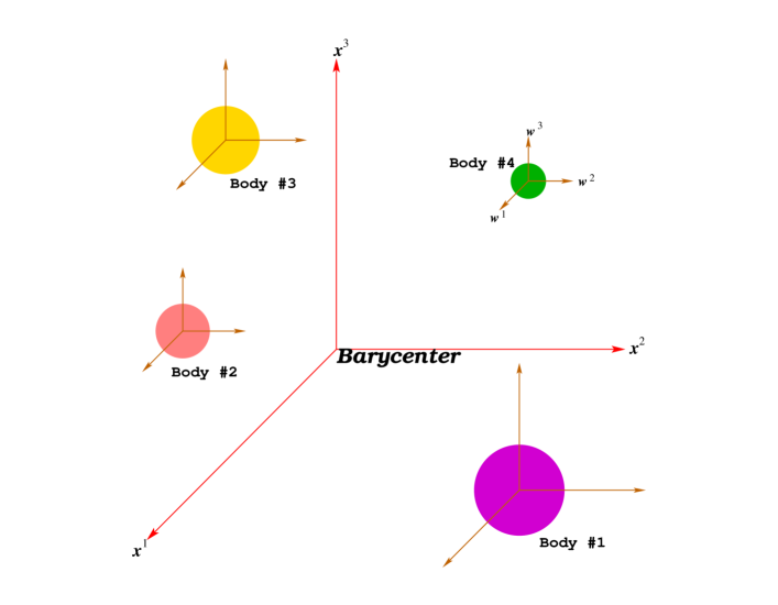
but in the most general case it has more complicated hierarchic structure which consists of a sequence of sub-systems each being comprised of Mp bodies where is a serial number of the sub-system (see Fig 2).
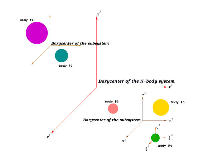
In its own turn each of the sub-systems can contain several sub-sub-systems, and so on. In order to describe dynamical behavior of the entire N-body system one needs to introduce a global 4-dimensional coordinate system. We denote such global coordinates , where is time coordinate and are spatial coordinates. Adequate description of dynamical behavior of the sub-systems of bodies and /or solitary celestial bodies requires introducing a set of local coordinates attached to each of the sub-systems (or a body) under consideration. Hence, a hierarchic structure of the coordinate charts in the N-body system repeats that of the N-body system itself and is fully compatible with mathematical notion of differentiable manifold [76, 77, 78]. We shall discuss local coordinates later in section 6.
Let us define the metric tensor perturbation with respect to the Minkowski metric (c.f. Eq. (3.3.4))
| (4.1.1) |
We demand that quantities and are bounded, and
| (4.1.2) |
where . Additional boundary condition must be imposed on the derivatives of the metric tensor to prevent appearance of non-physical radiative solutions associated with the advanced wave potentials [48]. It is written as
| (4.1.3) |
Eq. (4.1.3) is known as a ”no-incoming-radiation” boundary condition [48, 79]. In the case of an isolated astronomical system this condition singles out a causal solution of the D’Alembert wave equation depending on the retarded time only. Similar boundary conditions are imposed on the perturbation of the scalar field defined in Eq. (3.3.2)
| (4.1.4) |
| (4.1.5) |
In principle, the boundary conditions (4.1.3) and (4.1.5) are not explicitly required in the first post-Newtonian approximation for solving equations (3.5.5) – (3.5.9) because the gravitational potentials in this approximation are time-symmetric. However, they are convenient for doing calculations and are physically motivated. Therefore, we shall use the (radiative) boundary conditions (4.1.3) and (4.1.5) later on for giving precise definitions of the multipole moments of the gravitational field of the isolated astronomical system.
The global coordinates cover the entire space-time and they set up a primary basis for construction of the theory of relativistic reference frames in the N-body system [45]. In what follows, we shall assume that the origin of the global coordinates coincides with the barycenter of the N-body system at any instant of time. This condition can be satisfied after choosing a suitable definition of the post-Newtonian dipole moment of the N-body system and equating its numerical value to zero along with its first time derivative (see section 5.5). This can be always done in general relativity in low orders of the post-Newtonian approximation scheme if one neglects the octuple and higher-order multipole gravitational radiation [80]. In the scalar-tensor theory of gravity one has to take into account gravitational wave emission in the form of scalar modes [65] but it does not affect the first post-Newtonian approximation which is our main concern in the present paper. There are alternative theories of gravity which violate the third Newton’s law so that the dipole moment of an N-body system is not conserved even in the first post-Newtonian approximation [20] but we do not consider such extreme cases.
We shall also assume that spatial axes of the global coordinates do not rotate in space either kinematically or dynamically [59]. Spatial axes of a coordinate system are called kinematically non-rotating 101010Angular velocities of dynamic and kinematic rotations of a reference frame in classic celestial mechanics are equal. However, they have different values already in the first post-Newtonian approximation due to the presence of the relativistic geodetic precession caused by the orbital motion of the body. if their orientation is kept fixed with respect to a Minkowski coordinate system defined at the infinite past and at the infinite distance from the solar system 111111At the relativistic language the domain of the asymptotically-flat space-time is located both at the infinite distance and infinite past. This boundary consisting of null rays is called past null infinity [76].. Such kinematically non-rotating coordinate system can be built on the stellar sky by making use of quasars as reference objects with accuracy better than arcsec (see [81] and references therein). Quasars are uniformly distributed all over the sky and have negligibly small parallaxes and proper motions 121212Proper motion of an astronomical object in the sky is defined as its transverse motion in the plane of the sky being orthogonal to the line of sight of observer located at the barycenter of the solar system.. Thus, kinematically non-rotating coordinate system can be determined only through the experimental analysis of global properties of the space-time manifold including its global topology. This consideration reveals that the theory of reference frames in N-body system based on the assumption that the space-time is asymptotically-flat may be corrupted by the influence of some cosmological effects. Hence, a more appropriate approach to the reference frames taking into account that the background space-time is the Friedmann-Robertson-Walker universe is to be developed. We have done a constructive work in this direction in papers [27, 28] but the results of these papers are still to be matched with the post-Newtonian approximations.
Dynamically non-rotating coordinate system is defined by the condition that equations of motion of test particles moving with respect to these coordinates do not have any terms that might be interpreted as the Coriolis or centripetal forces [59]. This definition operates only with local properties of the space-time and does not require observations of distant celestial objects like stars or quasars. Dynamical definition of spatially non-rotating coordinates is used in construction of modern ephemerides of the solar system bodies which are based primarily on radar and laser ranging measurements to planets and Moon (see [21, 81, 82] and references therein). Because of the assumption that the N-body system under consideration is isolated, we can postulate that the global coordinates does not rotate at all in any sense.
4.2 The Metric Tensor and the Scalar Field in the Global Coordinates
The metric tensor is obtained by solving the field equations (3.5.5) – (3.5.9) after imposing the boundary conditions (4.1.2) – (4.1.4). We chose solution of the homogeneous equation (3.5.7) as . This is because describes rotation of spatial axes of the coordinate system but we assumed in the previous section that the global coordinates are not rotating. It yields solution of the other field equations in the following form
| (4.2.1) | |||||
| (4.2.2) | |||||
| (4.2.3) | |||||
| (4.2.4) | |||||
| (4.2.5) |
where
| (4.2.6) |
and the gravitational potentials , and can be represented as linear combinations of the gravitational potentials of each body, that is
| (4.2.7) |
Herein, the gravitational potentials of body A are defined as integrals taken over the volume of this body
| (4.2.8) | |||||
| (4.2.9) | |||||
| (4.2.10) | |||||
| (4.2.11) | |||||
| (4.2.12) | |||||
| (4.2.13) | |||||
| (4.2.14) |
where notation is used to define the volume integral
| (4.2.15) |
with being an integer, and – the volume of integration. Potential is determined as a particular solution of the inhomogeneous equation
| (4.2.16) |
with the right side defined in a whole space. Nevertheless, it proves out that its solution (see Eq. (4.2.10)) is spread out over volumes of the bodies only. It is worthwhile to emphasize that all integrals defining the metric tensor in the global coordinates are taken over the hypersurface of (constant) coordinate time . Space-time transformations can change the time hypersurface, hence transforming the corresponding integrals. This important issue will be discussed in section 7.
5 Multipolar Decomposition of the Metric Tensor and the Scalar Field in the Global Coordinates
5.1 General Description of Multipole Moments
In what follows a set of certain parameters describing properties of gravitational and scalar fields and depending on integral characteristics of the N-body system will be indispensable. These parameters are called multipole moments. In the Newtonian approximation they are uniquely defined as coefficients in Taylor expansion of the Newtonian gravitational potential in powers of where is the radial distance from the origin of a coordinate system to a field point. All Newtonian multipole moments can be functions of time in the most general astronomical situations. However, very often one assumes that mass is conserved and the center of mass of the system is located at the origin of the coordinate system under consideration. Provided that these assumptions are satisfied the monopole and dipole multipole moments must be constant.
General relativistic multipolar expansion of gravitational field is in many aspects similar to the Newtonian multipolar decomposition. However, due to the non-linearity and tensorial character of gravitational interaction proper definition of relativistic multipole moments is much more complicated in contrast to the Newtonian theory. Furthermore, the gauge freedom existing in the general theory of relativity clearly indicates that any multipolar decomposition of gravitational field will be coordinate-dependent. Hence, a great care is required for unambiguous physical interpretation of various relativistic effects associated with certain multipoles 131313See, for example, section 11 where we have shown how an appropriate choice of coordinate system allows us to eliminate a number of coordinate-dependent terms in equations of motion of spherically-symmetric bodies depending on the ”quadrupoles” defined in the global coordinate system. . It was shown by many researchers 141414For a comprehensive historical review see papers by [62], [83], [84] and references therein that in general relativity the multipolar expansion of the gravitational field of an isolated gravitating system is characterized by only two independent sets – mass-type and current-type multipole moments. In particular, Thorne [62] had systematized and significantly perfected works of previous researchers 151515Some of the most important of these works are [85, 86, 87, 88, 89]. and defined two sets of the post-Newtonian multipole moments as follows (see Eqs. (5.32a) and (5.32b) from [62])
| (5.1.1) | |||||
| (5.1.2) |
where numerical coefficients
| (5.1.3) | |||||
| (5.1.4) | |||||
| (5.1.5) |
and the multipolar integer-valued index runs from 0 to infinity. In these expressions is the effective stress-energy tensor evaluated at post-Newtonian order in the post-Newtonian harmonic gauge [62]
| (5.1.6) |
where
| (5.1.7) | |||||
| (5.1.8) | |||||
| (5.1.9) |
and , are gravitational potentials of the isolated astronomical system defined in Eqs. (4.2.7). Thorne [62] systematically neglected all surface terms in solution of the boundary-value problem of gravitational field equations. However, the effective stress-energy tensor falls off as distance from the isolated system grows as . For this reason, the multipole moments defined in Eqs. (5.1.1), (5.1.2) are to be formally divergent. This divergency can be completely eliminated if one makes use of more rigorous mathematical technique developed by Blanchet and Damour [63] for the mass multipole moments and used later on by Damour and Iyer [91] to define the spin multipoles. This technique is based on the theory of distributions [90] and consists in the replacement in Eqs. (5.1.1), (5.1.2) of the stress-energy pseudo-tensor defined in the entire space with the effective source which has a compact support inside the region occupied by matter of the isolated system [63, 91]. Blanchet and Damour proved [63] that formal integration by parts of the integrands of Thorne’s multipole moments (5.1.1), (5.1.2) with subsequent discarding of all surface terms recovers the multipole moments derived by Blanchet and Damour by making use of the compact-support effective source . It effectively demonstrates that Thorne’s post-Newtonian multipole moments are physically (and computationally) meaningful provided that one takes care and operates only with compact-support terms in the integrands of Eqs. (5.1.1), (5.1.2) after their rearrangement with the proper use of integration by parts of the non-linear source of gravitational field given by Eqs. (5.1.7)–(5.1.9). This transformation was done by Blanchet and Damour [63] who extracted the non-divergent core of Thorne’s multipole moments. We shall use their results in this paper.
In the scalar-tensor theory of gravity the multipolar series gets more involved because of the presence of the scalar field. This brings about an additional set of multipole moments which are intimately related with the multipolar decomposition of the scalar field outside of the gravitating system. We emphasize that definition of the multipole moments in the scalar-tensor theory of gravity depends not only on the choice of the gauge conditions but also on the freedom of conformal transformation of the metric tensor as was pointed out by Damour and Esposito-Farése [65] who also derived (in global coordinates) the set of multipole moments for an isolated astronomical system in two-parametric class of scalar-tensor theories of gravity. In this and subsequent sections we shall study the problem of the multipolar decomposition of gravitational and scalar fields both of the whole N-body system and of each body comprising the system in the framework of the scalar-tensor theory of gravity under discussion. In this endeavor we shall follow the line of study outlined and elucidated in [20, 62, 63, 65]. The multipole moments under discussion will include the sets of active, conformal and scalar multipole moments. These three sets are constrained by one identity (see Eq. (5.4.7)). Hence, only two of the sets are algebraically (and physically) independent. The multipole moments we shall work with will be defined in different reference frames associated both with an isolated astronomical system and with a single body (or sub-system of the bodies) comprising the isolated system. We call all these post-Newtonian moments as Thorne-Blanchet-Damour multipoles after the names of the researchers who strongly stimulated and structured this field by putting it on firm physical and rigorous mathematical bases. Let us now consider the multipole moments of the scalar-tensor theory of gravity in more detail.
5.2 Thorne-Blanchet-Damour Active Multipole Moments
Let us introduce the metric tensor potentials
| (5.2.1) | |||||
| (5.2.2) |
which enter and components of the metric tensor respectively. Furthermore, throughout this chapter we shall put and assume that the spatial metric component is isotropic, that is . Then, the field equations for these potentials follow from Eqs. (3.5.6), (3.5.8) and read
| (5.2.3) | |||
| (5.2.4) |
where we have introduced the active mass density
| (5.2.5) |
and the active current mass density
| (5.2.6) |
It is worthwhile to observe that in the global coordinates one has and . Hence, the expression (5.2.5) for the active mass density in these coordinates is simplified and reduced to
| (5.2.7) |
Solutions of Eqs. (5.2.3) and (5.2.4) are retarded wave potentials [66] determined up to the solution of a homogeneous wave equation and satisfying the boundary conditions (4.1.2) – (4.1.3). Taking into account that potentials and are in fact components of the metric tensor, solutions of Eqs. (5.2.3) and (5.2.4) can be written down as
| (5.2.8) | |||||
| (5.2.9) |
where designates a domain of integration going over entire space, and the gauge functions and are solutions of the homogeneous wave equation. We notice that because the densities and vanish outside the bodies the integration in Eqs. (5.2.8) and (5.2.9) is performed only over the volume occupied by matter of the bodies.
We take a special choice of the gauge functions as proposed in [63] (the only difference is the factor instead of in [63], coming from the field equation for component), namely
| (5.2.10) | |||||
| (5.2.11) |
Such gauge transformation preserves the gauge conditions (3.4.1) and also does not change the post-Newtonian form of the scalar multipole moments which will be discussed in the next section. Then one can show that potentials and can be expanded outside of the N-body system in a multipolar series as follows [63]
| (5.2.12) | |||||
where overdot denotes differentiation with respect to time . Eqs. (5.2.12) and (5.2) define the active Thorne-Blanchet-Damour mass multipole moments, , and the spin moments, , which can be expressed in the first PNA in terms of integrals over the N-body system’s matter as follows
| (5.2.14) | |||||
| (5.2.15) | |||||
| (5.2.16) |
As one can see the mass and current multipole moments of the scalar-tensor theory define gravitational field of the metric tensor outside of the N-body system as well as in general relativity [62, 63]. When these multipole moments coincide with their general relativistic expressions [63]. However, in order to complete the multipole decomposition of gravitational field in the scalar-tensor theory one needs to obtain a multipolar expansion of the scalar field as well.
5.3 Thorne-Blanchet-Damour Scalar Multipole Moments
In order to find out the post-Newtonian definitions of the multipole moments of the scalar field we again shall use the same technique as in [62, 63]. We take Eq. (3.1.5) and write it down with the post-Newtonian accuracy by making use of a new (scalar) potential
| (5.3.1) |
Then, Eq. (3.1.5) assumes the form
| (5.3.2) |
where the conventional notation for the Nordtvedt parameter [20] has been used and the scalar mass density is defined as
| (5.3.3) |
We can easily check out that in the global coordinates, where and , the scalar mass density is simplified and is given by
| (5.3.4) |
Solution of Eq. (5.3.2) is the retarded scalar potential
| (5.3.5) |
Multipolar decomposition of the potential (5.3.5) has the same form as in Eq. (5.2.12) with the scalar mass multipole moments defined as integrals over a volume of matter of the N-body system
| (5.3.6) |
We conclude that in the scalar-tensor theory of gravity the multipolar decomposition of gravitational field requires introduction of three sets of multipole moments – the active mass moments , the scalar mass moments , and the spin moments . Neither the active nor the scalar mass multipole moments alone lead to the laws of conservation of energy, linear momentum, etc. of an isolated system; only their linear combination does. This linear combination of the multipole moments can be derived after making conformal transformation of the metric tensor, solving the Einstein equations for the conformal metric, and finding its multipolar decomposition in the similar way as it was done in section 5.2.
5.4 Thorne-Blanchet-Damour Conformal Multipole Moments
Let us now define the conformal metric potential
| (5.4.1) |
The conformal field equations (3.1.7) in the quasi-harmonic gauge of Nutku (3.4.2) yield
| (5.4.2) |
where we have introduced a conformal mass density
| (5.4.3) |
which has been calculated directly from Eq. (3.1.7) by making use of the definition of the conformal metric (3.1.6) and the post-Newtonian expansions of corresponding quantities described in section 3.3. Remembering that in the global coordinates and one can simplify expression for the conformal mass density which assumes the form
| (5.4.4) |
This equation coincides precisely with the post-Newtonian mass density as it is defined in general relativity (see [20, 48] and [65] for more detail). The conformal current density is defined in the approximation under consideration by the same equation as Eq. (5.2.6), that is . The field equation for the conformal vector potential has the form (5.2.4), therefore .
Solution of Eq. (5.4.2) gives the retarded conformal potential
| (5.4.5) |
Multipolar expansion of conformal potentials and is done in the same way as it was done previously in section 5.2. It turns out that the conformal spin moments coincide with the active spin moments (5.2.16), and the expansion of the potential acquires the same form as that given in Eq. (5.2.12) but with all active multipole moments replaced with the conformal multipoles, , defined as follows
These conformal mass multipole moments coincide exactly with those introduced by Blanchet and Damour [63] who also proved (see appendix A in [63]) that their definition coincides precisely (after formal discarding of all surface integrals which have no physical meaning) with the mass multipole moments introduced originally in the first post-Newtonian approximation in general relativity by Thorne [62].
There is a simple algebraic relationship between the three mass multipole moments, , and in the global frame. Specifically, one has
| (5.4.7) |
We shall show later in section 6.3 that relationship (5.4.7) between the multipole moments obtained in the global coordinates for the case of an isolated astronomical N-body system preserves its form in the local coordinates for each gravitating body (a sub-system of the bodies) as well.
5.5 Post-Newtonian Conservation Laws
It is crucial for the following analysis to discuss the laws of conservation for an isolated astronomical system in the framework of the scalar-tensor theory of gravity. These laws will allow us to formulate the post-Newtonian definitions of mass, the center of mass, the linear and the angular momenta for the isolated system which are used in derivation of equations of motion of the bodies comprising the system. In order to derive the laws of conservation we shall employ a general relativistic approach developed in [66] and extended to the Brans-Dicke theory by Nutku [52].
To this end it is convenient to recast the field equations (3.1.2) to the form
| (5.5.1) |
where is an analog of the Landau-Lifshitz pseudo-tensor of the gravitational field in the scalar-tensor theory of gravity. This pseudotensor is defined by the equation
| (5.5.2) |
where is the (standard) Landau-Lifshitz pseudotensor [66] expressed in terms of the conformal metric and its derivatives.
The conservation laws are now obtained from Eq. (5.5.1)
| (5.5.3) |
They are a direct consequence of anti-symmetry of the right side of Eq. (5.5.1) with respect to the upper indices and . In what follows, we concentrate on the laws of conservation in the first post-Newtonian approximation only. Hence, we neglect the energy, linear and angular momenta taken away from the system by gravitational waves (see [65] where this problem has been tackled). For this reason, the conserved mass , the linear momentum , and spin of the isolated gravitating N-body system are defined as
| (5.5.4) | |||||
| (5.5.5) | |||||
| (5.5.6) |
In these definitions integration is performed over the whole space. Let us remark that the integrals are finite since in the first PNA and are of for large . Moreover, in this approximation the domain of integration can be reduced to the volume of the bodies comprising the system – observe that in (5.5.9) – (5.5.11) the functions under the integrals are compactly supported. Taking into account the asymptotic behavior of one can prove that the linear momentum can be represented as the time derivative of the function
| (5.5.7) |
which is interpreted as the integral of the center of mass. Hence,
| (5.5.8) |
where is a constant vector defining displacement of the barycenter of the N-body system from the origin of the global coordinate frame. One can chose and . In such case , and the center of mass of the N-body system will always coincide with the origin of the global reference frame. Such global reference frame is called barycentric. It is used in description of ephemerides of the solar system bodies, navigation of spacecrafts in deep space and reduction of astronomical observations of various types.
Direct calculations of the pseudotensor (5.5.2) with subsequent comparison with the conformal multipole moments (5.4) reveal that for the isolated system the post-Newtonian conserved quantities are
| (5.5.9) | |||||
| (5.5.10) | |||||
| (5.5.11) |
where by definition
| (5.5.12) |
and the integration is performed over the hypersurface of constant global coordinate time . It is evident from Eqs. (5.5.11) and (5.5.12) that it is the conformal moments, and , which define the conserved mass and linear momentum of the N-body system. The active monopole and dipole moments defined by Eq. (5.2.14) for are not consistent with the laws of conservation and, hence, can not serve to define the conserved quantities. We fix position of the center of mass (barycenter) of the N-body system in the global coordinates by equating conformal dipole moment of the system to zero, that is .
Now we are prepared to begin construction of a local coordinate system in the vicinity of a gravitating body or a sub-system of bodies which are members of the entire N-body system. For concreteness and for the sake of simplicity we shall focus on the construction of the local coordinate system around one body (Earth, planet, etc.).
6 Local PPN Coordinate System
6.1 Dynamic and Kinematic Properties of the Local Coordinates
Local coordinate system (local coordinates) is constructed in the vicinity of each body comprising the N-body system 161616Precise definition of body’s center of mass will be given in subsequent sections along with derivation of its equations of motion.. Thus, in principle, N local coordinate systems must be introduced in addition to one global coordinate system (see Fig. 1). In the case of the N-body system which is divided on sub-systems of bodies the number of the local coordinates increases in accordance with the underlying hierarchic structure of the N-body system (see Fig. 2). The principles of construction of the local coordinates are the same for any weakly gravitating body (a sub-system of bodies). For this reason, it is sufficient to work out description of only one local coordinate system, , as the other local coordinate charts must have a similar structure [58]. For practical applications in the solar system the most important local coordinates are associated with the Earth and they are called geocentric coordinates. Local coordinates are not asymptotically Minkowskian far away from the body because the gravitational field of the body under consideration must smoothly match with the gravitational field of external bodies.
We assume that each body consists of matter which admits continuous distribution of mass density, anisotropic stresses and internal velocity field. If one had “turned off” gravitational field of all external bodies (Moon, Sun, planets) but the gravitational field of the body under consideration (Earth), it would be described by a set of the (internal) multipole moments defined by equations given in previous section. However, we can not neglect gravitational field of the external bodies if one wants to take into account classic [76, 92] and relativistic effects associated with tides [72, 93]. The tidal deformation of the body will be comprehensively large, for example, at the latest stage of coalescence of neutron stars in binary systems emitting gravitational radiation and is to be taken into account in calculations of the templates of gravitational waves being emitted by such systems. We also know that already in the Newtonian limit this external gravitational field reveals itself in the vicinity of the Earth as a classical tidal force [76]. Gravitational potential of the tidal force is represented as a Taylor series with respect to the local geocentric coordinates with time-dependent coefficients which are called external (tidal) multipole moments [94]. This series usually starts in the Newtonian approximation from the second order (quadratic) term because the monopole and dipole external multipole moments are not physically associated with the tidal force. In general relativity this monopole-dipole effacing property of the external gravitational field is retained in the post-Newtonian approximation as a consequence of the Einstein principle of equivalence (EEP) [20, 66, 76]. In particular, EEP suggests that it is possible to chose such (local) coordinates that all first derivatives of the metric tensor (i.e., the Christoffel symbols) vanish along a geodesic world line of a freely falling particle [40]. This is equivalent to making a suitable coordinate transformation on the space-time manifold from the global to local frame [77, 78]. In general relativity this property of EEP is also valid for a self-gravitating body moving in external gravitational field of other bodies. The original proof was given in [94, 95, 96] and elaborated on later in a series of papers by other researchers [42, 43, 45, 61, 69, 70].
As contrasted with general relativity the scalar-tensor theory of gravity has a scalar (helicity-0) component of the gravitational field which can not be eliminated by a coordinate transformation to the local frame of the body being in a free fall. This is because the scalar field does not change its numerical value under pointwise coordinate transformations and can not be eliminated if it has a non-zero value on space-time manifold. It means that scalar fields do not obey the principle of equivalence and the gravitational field in the scalar-tensor theory can not be reduced in the local coordinate system to the tidal field only. In particular, this was the reason why Einstein had rejected a theory of gravity based exceptionally on a scalar field (for more detail see [20, 76]).
This argument makes it clear that in order to incorporate a local coordinate system to the standard PPN formalism [16] –[20] one needs to know the nature of the fundamental fields (scalar, vector, tensor, spinor, etc.) present in the theory because these fields have different behavior under coordinate transformations. To construct a local coordinate system, solution of the field equations for all fundamental fields must be found directly in the local coordinate system. Then, this solution must be matched to the solution of the same equations in the global coordinates and the transformation laws of the additional fields must be used along with the transformation law of the metric tensor in order to find relativistic space-time transformation between the global and local coordinate systems. Nonetheless, one has to keep in mind that the scalar field is not observed directly but is organically incorporated to the metric tensor which obeys to EEP. It means that the scalar field and its first derivative at each point of the manifold can be absorbed in the metric tensor and its first derivatives. Thus, the metric tensor in the origin of the local coordinates can be reduced to the Minkowski metric as long as the body’s gravitational field is not to be a matter of concern.
We demand that the origin of the local coordinates coincides with the body’s center of mass at any instant of time. This requires a precise definition of the center of mass of each body with respect to its local coordinates. But when one takes into account the post-Newtonian corrections, the notion of the body’s center of mass becomes ambiguous because it can be chosen in several different ways depending on what kind of definition of the internal dipole moment of the body in the multipolar expansion of the local metric tensor is chosen. We have proven by straightforward calculations that it is the conformal dipole moment (5.5.10) which gives a physically correct definition of the body’s center of mass because only this moment allows to derive equations of translational motion of the body which does not contain self-accelerated terms violating the Newton’s third law of action-counteraction. This property of the conformal moment is closely related to its conservation for an isolated system of N bodies as demonstrated in section 5.5.
In general, the body (Earth) as a part of the N-body system is not isolated and interacts gravitationally with other bodies (Moon, Sun, etc.). For this reason, the second and higher order time derivatives of the conformal dipole moment of the body are not equal to zero by themselves. It means that there is a local force exerted on the body by external gravitational field which prevents its linear momentum (the first time derivative of the body’s dipole moment) to conserve. Nevertheless, it is possible to prove that all time derivatives of the body’s dipole moment can be kept equal to zero if one chose the origin of the local coordinates to move not along a geodesic world line. This goal is achieved by making use of a specific choice of external dipole moment in the multipolar expansion of the homogeneous solution of the gravitational field equations (see section 9.4). The correct choice of the body’s center of mass allows us to eliminate the ill-behaved coordinate-dependent terms in the equations of motion of the body and facilitates discussion of the strong equivalence principle’s violation (the Nordtvedt effect) for extended bodies.
We admit that the local coordinates can be, in general, dynamically rotating. It means that translational equations of motion of a test particle written down in the local coordinates can include the Coriolis and centrifugal forces. If one excludes the dynamical rotation of the local coordinates, their spatial axes will slowly rotate in the kinematic sense with respect to the spatial axes of the global coordinates [13, 14]. This effect is called a geodetic precession and it obeys the law of parallel transport of vectors on curved space-time manifold [76]. Nowadays, the IAU recommends to use a kinematically-nonrotating geocentric system which spatial axes are anchored to distant quasars used as reference points of the international celestial reference system (ICRS) (see [97] for more detail). The metric tensor of the kinematically-nonrotating geocentric coordinates has an external dipole moment in component of the geocentric metric tensor describing the dynamical rotation of the spatial axes of the geocentric coordinates. This term would be zero if the geocentric coordinates were chosen to be dynamically nonrotating. The angular velocity of the dynamical rotation is equal to that of the geodetic precession and is fixed by the corresponding IAU resolution. At this step of development of our formalism we shall not specify the angular velocity of the dynamical rotation in order to keep the formalism as general as possible.
6.2 The Metric Tensor and the Scalar Field in the Local Coordinates
We denote the local (for example, geocentric) coordinates by where stands for the local coordinate time. All quantities related to the (central) body around which the local coordinate frame is constructed will be labelled by subindex B standing for “body”. We are looking for the solution of the field equations (3.5.5) – (3.5.6) inside a world tube containing the world line of the body’s center of mass and spreading up to the nearest external body, so that the only source of matter inside the region covered by the local frame is the matter of the central body. Thus, the right side of equations (3.5.5) – (3.5.9) contains the energy-momentum tensor of the body’s matter only. Spatial domain of applicability of the local coordinates can be extended after finding the space-time transformation from local to global coordinates [61].
Solution of the differential equations (3.5.5) – (3.5.6) is a linear combination of general solution of the homogeneous equation and a particular solution of the inhomogeneous equation. For example, solution for a scalar field in the local coordinates is written as
| (6.2.1) |
whereas the metric tensor, , is given in the form
| (6.2.2) |
where terms with sub-index B refer to the central body (Earth) and describe the (internal) solution of the inhomogeneous equations, terms with sub-index E refer to the external bodies (Moon, Sun, etc.) and describe the (external) solution of the homogeneous equations, and terms with sub-index C (which stands for coupling) arise because of the non-linearity of the gravity field equations for the metric tensor. One notices that in the first post-Newtonian approximation the coupling terms appear only in component of the metric tensor. We do not impose any other specific limitations on the structure of the metric tensor in local coordinates. All information about its structure can be obtained from the solution of the field equations (3.5.5) – (3.5.9). We draw attention of the reader that we put a hat over all quantities referred to the local coordinates . This is because functional dependence of one and the same quantity looks different in different coordinates. For example, for any scalar function and coordinate transformation one has while differs from [77, 78].
6.2.1 The Scalar Field: Internal and External Solutions
Eq. (3.5.5) gives internal, , and external, , solutions for the scalar field in the following form
| (6.2.3) | |||||
| (6.2.4) |
Here are external STF multipole moments in the multipolar decomposition of the scalar field generated by the bodies which are external with respect to the central body. These external moments are functions of the local time only. The internal solution describes the scalar field which is generated by the central body only.
6.2.2 The Metric Tensor: Internal Solution
The boundary conditions imposed on the internal solution for the metric tensor are identical with those given in Eqs. (4.1.2) – (4.1.3). For this reason the internal solution for the metric tensor has a form which is similar with that obtained in the global coordinates where all quantities must be referred now only to the central body. We obtain
| (6.2.5) | |||||
| (6.2.6) | |||||
| (6.2.7) | |||||
| (6.2.8) |
where all gravitational potentials of the central body are taken over the volume of the body’s matter defined as a cross-section of the body’s world tube with the hypersurface of constant local coordinate time . Specifically, one has
| (6.2.9) | |||||
| (6.2.10) | |||||
where
| (6.2.12) | |||||
| (6.2.13) | |||||
| (6.2.14) | |||||
| (6.2.15) | |||||
| (6.2.16) |
the symbol is the velocity of the body’s matter with respect to the origin of the local coordinates, and we have introduced a special notation
| (6.2.17) |
for integrals over the body’s volume. We emphasize once again that the integrand of is a function which is taken over the hypersurface of constant time .
The local metric given by Eqs. (6.2.3), (6.2.5) – (6.2.8) must obey the gauge condition (3.4.1) which yields
| (6.2.18) |
This is the only gauge condition which can be imposed on the local metric in the first post-Newtonian approximation. We note that Eq. (6.2.18) is satisfied due to the validity of the equation of continuity (3.3.19).
6.2.3 The Metric Tensor: External Solution
Solution of the homogeneous field equations for the metric tensor given in this section is based on and extends the multipolar formalism for description of vacuum gravitational fields developed in [94, 98]. Brief introduction to this formalism is given in Appendix A. Boundary conditions imposed on the external solution must ensure its convergency on the world line of the origin of the local coordinates where . However, the external solution for the metric tensor diverges as the radial distance from the origin of the local coordinates grows. This is because of the gravitational field of external bodies which does not asymptotically vanish in the local coordinates for large [94, 98].
Explicit form of the external solution for the linearized metric tensor perturbation in local coordinates is given by
| (6.2.19) | |||||
| (6.2.20) | |||||
| (6.2.21) | |||||
where is the angular velocity of kinematic rotation of the local frame with respect to the global coordinates, is the velocity of the local frame with respect to the local frame moving along geodesic world line (see below), and either symbol “” or the round brackets around indices denote symmetry with respect to the indices, for instance, . In (6.2.19) – (6.2.3) we keep only the terms of and which are relevant for the discussion of Newtonian geodesics. It is worth to notice that external solutions for the metric tensor in local coordinates contain monopole terms and . Term defines the unit of measurement of the coordinate time at the origin of the local frame and defines the unit of measurement of spatial distances with respect to the international system of units. Both these terms could be equated to zero from the very beginning but we prefer to keep them in our equations for generality. This is because the IAU resolutions [14] explicitly introduce the non-zero values of and and this is why we are interested in the impact of these functions on the PPN theory of reference frames 171717Functions [99, 100] (see also [101, 102] for detailed theoretical review on the relativistic time scales in the solar system..
In order to understand physical meaning of various components of the external solution for the metric tensor in the local coordinates it is instructive to write down the Newtonian equation of motion of a test particle falling freely in the field defined by the external metric. This equation is a geodesic world line so that after calculation of the Christoffel symbols one has particle’s acceleration
where and we have neglected the post-Newtonian corrections. First two terms in the right side of this equation, , describe kinematic acceleration of the particle with respect to the coordinate system moving along geodesic. The third term, , in the right side of Eq. (6.2.3) is the famous Coriolis acceleration [103] caused by motion of the particle and rotation of spatial axes of the local frame with angular velocity . The forth term, , in the right side of Eq. (6.2.3) is acceleration due to the non-uniform rotation of the local frame. The fifth term, , describes a centrifugal acceleration of the particle. The sixth term, , is a quadrupole tidal acceleration due to the presence of external gravitational field from other bodies besides the central one. Last term in the right side of Eq. (6.2.3) is the tidal acceleration due to the higher order multipoles of the external gravitational field of other bodies. It is interesting to note that the centrifugal and the quadrupole tidal accelerations have similar structure. The difference, however, is that the matrix of the centrifugal acceleration, , is not trace-free in contrast to the tidal matrix, . However, the trace-free part of can be singled out and absorbed to the definition of .
It is convenient to construct the external part of the metric tensor in such a way that makes it Minkowskian (orthogonal) at the origin of the local coordinates. This can be achieved if one chooses function . This condition also allows us to give a unique interpretation of the dipole term as equal to the inertial force per unit mass exerted on the free falling particle due to the accelerated motion of the local frame under consideration with respect to the geodesic world line. In other words, the metric tensor with and specifies a local coordinate system such that its origin moves with acceleration with respect to a geodesic world-line defined on the background space-time which is determined exclusively by the external part of the metric tensor. We also notice that the dipole term in Eq. (6.2.21) is just a post-Newtonian correction to and would also destroy orthogonality of spatial axes of the local frame at its origin. Thus, in addition to the condition, , we also demand, . Therefore, any post-Newtonian corrections to the equations of motion of the origin of the local coordinates are hidden in the inertial acceleration in Eq. (6.2.19).
A set of eleven external STF multipole moments , , , , , , , , , (we omit for simplicity, i.e. , etc.) is defined on the world line of the origin of the local coordinates so that these multipoles are functions of the local coordinate time only. Furthermore, the external multipole moments are symmetric and trace-free (STF) objects with respect to any of two indices, and they are transformed as tensors with respect to linear coordinate transformations. In what follows, we shall assume that the angular velocity of rotation of the local frame, , is so small that the metric tensor component is comparable with that . For this reason, we shall neglect all terms which are either quadratic with respect to or are products of with one of each of the other components, , or . Only linear with respect to terms and their first derivatives will be retained in our calculations.
Imposing the gauge conditions (3.4.1) on the metric tensor given by Eqs. (6.2.19) – (6.2.3) reveals that only 7 from 11 external multipole moments are algebraically independent. More specifically, the gauge condition (3.4.7) leads to the following relationship between the moments
| (6.2.24) |
Three other relationships are obtained after accounting for Eq. (6.2.24) in the gauge condition (3.4) which yields
| (6.2.25) |
and
| (6.2.26) | |||||
| (6.2.27) | |||||
| (6.2.28) |
Eqs. (6.2.24) – (6.2.28) allow us to eliminate the external multipole moments from the local metric so that the space-time and space-space components of the external metric tensor assume the form
Remaining multipole moments , , , , , , and the angular velocity of rotation, , can not be constrained by imposing the gauge conditions. However, a residual gauge freedom described by differential Eq. (3.4.9) allows us to find further limitations on the remaining 7 sets of the multipole moments which are explicitly shown in the right side of Eqs. (6.2.3) and (6.2.3). Exclusion of the residual degrees of freedom makes it clear which multipole moments are in fact physically relevant, that is can not be excluded by infinitesimal coordinate transformations .
In order to exclude the external multipoles, which do not carry out information about gravitational degrees of freedom, we shall make use of a well-known property of the gauge-invariance of the (linearized) Riemann tensor under infinitesimally small coordinate transformations (see Box 18.2 in [76])
| (6.2.31) |
Eq. (6.2.31) must be understood as invariance of the functional form of the Riemann tensor after making an infinitesimally small gauge transformation. Computing all components of the Riemann tensor, which are functions of the external metric tensor (6.2.19), (6.2.3) and (6.2.3) only, one finds (see Appendix B.2) that the external part of the Riemann tensor depends only on four sets of the external multipole moments , , and . However, one can notice that the multipoles and enter Eq. (B.2) only in the form of a linear combination which can not be split algebraically. This means that only three sets of the external moments have a real physical meaning. In what follows, we shall choose , , and as the primary external multipoles. Other multipole moments , , and can be chosen arbitrary which reflects the presence of 4 residual gauge degrees of freedom generated by the coordinate transformation confined by Eq. (3.4.9).
Hereafter we assume that the angular velocity of rotation of the local frame
| (6.2.32) |
which gives . This assumption greatly simplifies subsequent calculations without missing any significant physics. We have to notice, however, that rotating local coordinate systems have a great practical value for satellite geodesy and global positioning system (GPS) [104].
Various authors used the residual gauge freedom differently. We shall follow the convention accepted in papers [15, 45, 69, 94] and postulate 181818We draw attention of the reader that in the standard PPN formalism [20] and in the global coordinates the space-space components of the metric tensor are always diagonal in standard gauge. However, here we discuss the local coordinates which admit more general degrees of freedom than the global ones. Hence, our postulate is not redundant. that the space-space components of the local metric tensor must form a diagonal matrix proportional to the Kronecker symbol . It allows to simplify the non-linear term in Eq. (3.5.6) for the time-time component of the metric tensor by making use of the Laplace equation for function which converts the non-linear term to that having a compact support, that is . In order to diagonalize one chooses the external multipoles , as follows
| (6.2.33) |
| (6.2.34) |
for all . Furthermore, we chose
| (6.2.35) |
for all with but the monopole moment which is left arbitrary 191919Restrictions (6.2.33) – (6.2.35) on the external multipoles result of the requirement that the metric tensor must be diagonal in the entire domain of validity of the local coordinates but not in a single point.. We preserve some gauge freedom and do not fix the external multipoles ().
Finally, the external metric tensor assumes the following simple form
| (6.2.36) | |||||
| (6.2.38) |
where we still keep the (time-dependent) monopole term .
Now we can compute component of the external metric tensor up to the post-Newtonian order by making use of Eq. (3.5.6). Its the most general solution is determined up to that of a homogeneous wave equation which we shall assume to be incorporated to the post-Newtonian correction to the multipole moments defined by Eq. (6.2.36). Hence, we obtain
It is interesting to note that summation in the first two terms in the right side of Eq. (6.2.3) was originally started from (see Eqs. (6.2.4) and (6.2.19)). However, product of a harmonic polynomial with the monopoles and represent a homogeneous solution of the Laplace equation and, for this reason, can be absorbed by the Newtonian-like polynomial in Eq. (6.2.36) by means of re-definition of the multipoles . This is possible because the mathematical structure of the multipoles as functions of the parameters of the external bodies has not yet been specified. Our remark helps to realize that the influence of the scalar field on the external solution of the metric tensor in the local coordinates starts from quadratic, with respect to coordinates , terms only. External scalar field can not be eliminated by pointwise coordinate transformation but it enters to the external metric tensor in such a way that it can be absorbed to the multipole moments of the metric tensor gravitational field. Hence, the external multipoles do not contribute linearly to the equations of translational motion of test particles and extended bodies – only their non-linear combination is observable (see section 9).
6.2.4 The Metric Tensor: The Coupling Terms
The coupling terms in the metric tensor in local coordinates are given as a particular solution of the inhomogeneous equation (3.5.6) with the right side taken as a product of the internal and external solutions found on previous step of the approximation procedure. Solving Eq. (3.5.6) yields the coupling terms of the metric tensor in the local coordinates
This completes derivation of the metric tensor in the local coordinates.
6.3 Multipolar Decomposition of the Body’s Gravitational Field in the Local Coordinates
The local coordinates are introduced in the vicinity of each of the gravitating body comprising the N-body system. We consider one of them and call it the ”central” body which is indexed by the letter ’B’. This body, for example, can be the Earth and the local coordinates in such case are called the geocentric coordinates [14, 15]. Gravitational field of the central body taken alone, that is when all other (external) bodies are ignored, is described in the local coordinates in terms of the metric tensor and scalar field which depend on the internal field potentials , , , etc., defined in Eqs. (6.2.9) – (6.2.15). Multipolar decomposition of the internal metric tensor of the central body is totally equivalent to the procedure of multipolar decomposition of the gravitational field of the N-body in global coordinates described in section 11.3. However, from the point of view of precise theory the central body is not gravitationally isolated from the other bodies of the N-body system because it interacts with them gravitationally. This interaction brings about the coupling terms to the metric tensor in the local coordinates which can contribute to the numerical values of the body’s multipole moments in the multipolar decomposition of the local metric tensor. The presence of the coupling terms introduces a post-Newtonian ambiguity of the multipolar decomposition of gravitational field in the local coordinates and puts a question about what specific definition of the multipole moments of the central body must be used in deriving translational and rotational equations of motion of the body in the gravitational field of N-body system. This problem was seemingly pointed out for the first time by Thorne and Hartle [94].
Solution of this problem can be found only by doing complete calculations of the equations of motion of the central body with taking into account all its multipoles. One has two possibilities: either to include or to exclude the contribution of the coupling terms to the multipole moments of the body and we have explored both of them. It turns out the final form of the equations of motion can be significantly simplified if the coupling terms are included to the definition of the multipole moments. In fact, if one excludes the contribution of the coupling terms to the body’s multipoles it produces a lot of additional terms in the equations of motion but all these terms can be eliminated after a suitable re-definition of the multipole moments. By inspection one can check that the final form of such renormalized equations of motion coincides with that which would be obtained if one included contribution of the coupling terms in the local metric tensor to the definition of the multipole moments of the central body from the very beginning. The significantly simple form of the renormalized equations of motion is a direct indication that the coupling terms must be included to the definition of the multipole moments of the body in the local coordinates. This resolves the Thorne-Hartle ambiguity [94] in the definition of the multipole moments.
Thus, the formal procedure of the multipolar decomposition of the gravitational field in the local coordinates is based on the same field equations (5.2.3), (5.3.2) and (5.4.2) for active, scalar and conformal potentials whose right sides depends on the active, scalar and conformal mass densities defined by Eqs. (5.2.5), (5.3.3) and (5.4.3) respectively. All these densities depend on the trace of the space-space component of the metric tensor, , and the scalar field, . In accordance with our procedure of definition of the multipole moments in the local coordinates, these functions must include the contribution of the external gravitational and scalar fields. In other words, computation of the mass densities in Eqs. (5.2.5), (5.3.3) and (5.4.3) in the local coordinates must be relied upon the trace of the metric tensor, , defined by the sum of Eqs. (6.2.8) and (6.2.38), and the scalar field, , defined by the sum of Eqs. (6.2.3) and (6.2.5). Solving Eqs. (5.2.3), (5.3.2), (5.4.2) with the mass densities defined herewith and expanding the metric potentials in the multipolar series yields the multipole moments of the central body in the local coordinates.
In section 4 we have constructed three sets of the mass multipole moments – active, scalar, and conformal. The same type of multipoles presents in the local coordinates as well. The active STF mass multipole moments of the central body are
where denotes the volume of the central body under consideration and the active mass density in the body’s interior is defined as
| (6.3.2) |
where is the gravitational potential of the body given by Eq. (6.2.9).
The scalar STF mass multipole moments of the body are defined as
where the scalar mass density of the body’s matter is defined by
| (6.3.4) |
The conformal STF mass multipole moments of the body are
with the conformal mass density of the body’s matter defined as
| (6.3.6) |
The conformal density does not depend on the PPN parameters and .
The current density is defined in the local coordinates by
| (6.3.7) |
and the spin multipole moments of the body are determined by the formula 202020We discuss the post-Newtonian definition of body’s spin in section 10.
| (6.3.8) |
It is important to emphasize that the algebraic relationship (5.4.7) preserves its form for the set of the mass multipole moments taken for each body separately, that is
| (6.3.9) |
Validity of this relationship can be checked out by a straightforward calculation. We also draw attention of the reader that the hypersurface of the integration in Eqs. (6.3), (6.3), (6.3) is that of the constant local coordinate time which does not coincide with the hypersurface of the constant time in the global coordinates (see Fig. 3).
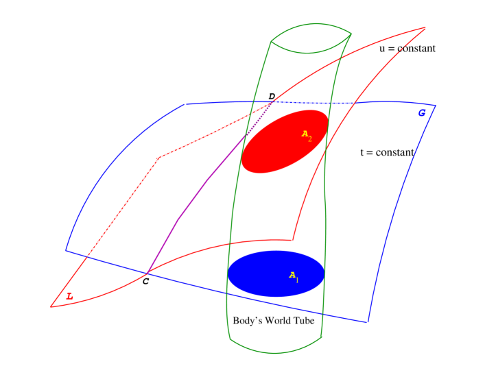
This remark is of a great importance in the matching procedure of the local and global coordinates discussed in next section. It will be also important in section 11 for correct derivation of equations of motion of the body which requires comparison of the definition of the multipole moments of the body in the local coordinates used in this paper and that in the global coordinates used by some other authors 212121See section 11 for more detail..
7 Parametrized Post-Newtonian Transformation from Local to Global Coordinates
7.1 Preliminary Remarks
General relativistic post-Newtonian coordinate transformation from local, , to global, , coordinates are used in standard algorithms of data processing of various astronomical observations to reduce the observable quantities to the barycentric coordinates of the solar system [21, 82] where they are “stored” (catalogued) at a certain astrometric epoch recommended for the international usage by the IAU. The most commonly used epochs are J2000 and B1950 (i.e. instantaneous orientation of the barycentric coordinates fixed by the position of the vernal equinox as it was located on the sky in 2000AD or 1950AD). Post-Newtonian coordinate transformation from the local to global frame is an inalienable part in the procedure of derivation of the general relativistic equations of motion of test and/or extended bodies in the solar system [1, 41, 42, 43, 45, 56, 57, 58, 59, 60, 61, 69, 70, 105, 106] as well as compact relativistic stars in binary systems emitting gravitational waves [67, 79, 95, 96, 107, 108]. It is widely accepted that scalar fields must exist since they provide elegant explanation for various effects and phenomena encountered by modern theoretical physics of fundamental particle interactions, gravitation and cosmology [109]. Therefore, it is natural to generalize the existing form of the general relativistic post-Newtonian transformation from the local to global coordinates to make them fully compatible with the scalar-tensor theory of gravity. Solution of this problem in terms of the PPN parameters and is displayed in the present section.
The PPN coordinate transformations from the local (geocentric) coordinates to global (barycentric) coordinates can be found by making use of the asymptotic expansion matching technique [114] as proposed in [95, 96]. The metric tensor and the scalar field are solutions of the field equations which are expressed in the form of two different post-Newtonian expansions in the global and local coordinates. These two expansions of the metric tensor and the scalar field must match smoothly in the spatial domain where both coordinate charts overlap. This matching domain is originally defined as a region in which the post-Newtonian expansion of the metric tensor and scalar field is not divergent. In the case of a weak gravitational field this domain extends from the origin of the local coordinates associated with a central body (Earth) up to the next closest celestial body (Moon) 222222In the N-body system comprised of neutron stars and/or black holes the local coordinates would overlap with the global ones in the so-called buffer region in which the gravitational field of both the neutron star/black hole and the external bodies is weak. More details on this subject can be found in papers [94]–[96].. However, after the structure of the PPN coordinate transformation is found the domain of applicability of the local coordinates can be stretched out up to much larger distances (see text below after Eq. (7.3) and papers [47, 61, 105] for more detail).
Special relativistic transformation from local to global coordinates is linear and takes into account only kinematic aspects of the transformation, i.e. that the local frame moves with respect to the global one with constant velocity. The special relativistic (Poincaré-Lorentz) transformation is described at each instant of time by 10 parameters characterizing the intrinsic properties of flat space-time which is tangent to curved space-time manifold at any point on the world line of the origin of the local coordinates [48, 66, 76]. These parameters include 4 space and time translations, 3 spatial rotations, and 3 Lorentz boosts depending on the velocity of the origin of the local frame with respect to the global coordinates. General relativity generalizes the Poincaré-Lorentz transformation by accounting for the presence of dynamic effects (acceleration) in the motion of the local frame as well as for the effects of the external gravitational field of the other bodies and the background curvature of the space-time. It was shown (see, e.g., [43, 45, 95, 96] and references therein) that in general relativity the post-Newtonian coordinate transformation from local to global coordinates is non-linear, has more than 10 parameters, and all parameters depend on time. Scalar-tensor theory of gravity brings about additional complications to the relativistic theory of reference frames caused by the dependence of the post-Newtonian transformation on the scalar field which is described by two more parameters, and . However, scalar-tensor theory does not change general structure of the parametrized post-Newtonian (PPN) transformation which remains the same as that used in general theory of relativity.
The PPN coordinate transformation between the global and local coordinates belongs to the class of transformations which must comply with the gauge condition (3.4.1). Therefore, one begins with finding of the most general structure of such coordinate transformations. As soon as this structure is known it can be further specialized by reducing the number of the gauge degrees of freedom by making use of the residual gauge transformations and matching technique applied for establishing a one-to-one correspondence between two asymptotic expansions of the metric tensor and scalar field written down in the global and local coordinates. This procedure allows us to arrive to a single, ingenious form of the PPN coordinate transformation. We shall show that the PPN transformation from local to global coordinates can be represented as a power series expansion with respect to two small parameters, and , where and are distances from the origin of the local coordinates (the central body) to matching point in space and to the other (external) gravitating body respectively. Coefficients of the power series expansion are symmetric and trace-free (STF) multi-index functions of time which are determined simultaneously with the external multipole moments, , , , etc., of the local metric in the course of the matching procedure. The STF coefficients of the PPN coordinate transformation are functions of the local coordinate time and are “pinned down” to the origin of the local coordinates. The matching procedure shows that the STF coefficients of the most general form of the PPN coordinate transformation couples linearly with the external STF multipole moments of the local metric tensor entering Eqs. (6.2.19) – (6.2.3) so that the matching allows to derive a set of equations defining only their algebraic sum. This reflects existence of the residual gauge freedom which can be used in order to simplify the structure of the PPN coordinate transformation and/or that of the metric tensor in local coordinates. We have used this gauge freedom already in section 6.2.3 to suppress the number of the external multipole moments which have no physical significance. Elimination of the non-physical multipole moments from the metric tensor leads to more simple structure of the PPN transformations as well. This issue is discussed in the next sections in more detail.
7.2 General Structure of the Coordinate Transformation
The most general structure of the coordinate transformation from the local, , to global, , coordinates in the weak-field and slow-motion post-Newtonian approximation is given by two equations:
| (7.2.1) | |||||
| (7.2.2) |
where and are the post-Newtonian corrections to the Galilean transformation, , and is the position of the origin of the local frame at time with respect to the origin of the global coordinates. We shall prove later on that the origin of the local coordinates can be always chosen at any instant of time at the center of mass of the body (Earth, Sun, planet) around which the local coordinate chart has been constructed. In what follows, we shall denote velocity and acceleration of the origin of the local coordinates as and respectively, where here and everywhere else the overdot must be understood as a time derivative with respect to time .
Pointwise matching equations for the scalar field, the metric tensor, and the Christoffel symbols are given by their general laws of a coordinate transformation [76, 77, 78]
| (7.2.3) | |||||
| (7.2.4) | |||||
| (7.2.5) |
One recalls that component of the metric tensor does not contain terms of order because we have assumed that both the global and the local frames are not rotating. This fact, being used in Eq. (7.2.4), implies that function from Eq. (7.2.1) must be subject to the following restriction: . This is a partial differential equation which can be integrated so that function can be represented as
| (7.2.6) |
where and are analytic, but in all other aspects yet unspecified, functions 232323Notice that function depends only on time ..
Let us now use the gauge conditions (3.4.3) in order to impose further restrictions of the PPN functions and from Eqs. (7.2.1) and (7.2.2). The gauge conditions can be written in arbitrary coordinates as an exact equality
| (7.2.7) |
The law of transformation of the Christoffel symbols, Eq. (7.2.5), being substituted to Eq. (7.2.7) yields a partial differential equation of the second order
| (7.2.8) |
which describes any possible freedom of the PPN transformation in the quasi-harmonic gauge of the scalar-tensor theory of gravity. Let us now substitute functions and from Eqs. (7.2.1) and (7.2.2), and from Eq. (7.2.6) to Eq. (7.2.8). One obtains
| (7.2.9) | |||||
| (7.2.10) |
General solution of these elliptic-type equations can be written in the form of the power series expansion in terms of the scalar and vector spherical harmonics (see appendix A for more detail). Furthermore, solution for functions and in Eqs. (7.2.9) and (7.2.10) consist of two parts – general solution of the homogeneous Laplace equation and a particular solution of the inhomogeneous elliptic equation. We shall omit that part of the solution of the homogeneous equation which is singular at the origin of the local coordinates, that is at the point . In general, such ill-behaved terms can be present in other alternative theories of gravity which violate the law of conservation of linear momentum. But in the scalar-tensor theory of gravity such ill-behaved functions do not appear in the geocentric metric and we do not need singular terms in the coordinate transformations (7.2.1) and (7.2.2) to match the scalar field and the metric tensor in two coordinate systems. Integration of equations (7.2.9) and (7.2.10) results in
| (7.2.11) | |||||
| (7.2.12) |
where functions and are solutions of the homogeneous Laplace equation. These solutions can be written in the form of harmonic polynomials
| (7.2.13) | |||||
| (7.2.14) |
where the coefficients , , , and of the polynomials are different multi-index STF functions. These functions are defined on the world line of the origin of the local coordinates and depend only on the global time . Explicit form of these functions will be obtained in the process of matching of the global and local metric tensors as well as the scalar field. Notice that we have denoted all, yet unknown STF functions in Eqs. (7.2.13) and (7.2.14) by capital calligraphic letters, while the STF multipole moments in the expressions for the local metric, Eqs. (6.2.36) – (6.2.38), and the scalar field (6.2.4) have been denoted by capital roman letters. This is supposed to help to distinguish the STF functions having different origin. We also emphasize that the specific form of functions in the coordinate transformations (7.2.11) and (7.2.12) is the most general one which preserves the gauge conditions (7.2.7) and allows us to analyze the residual gauge freedom in construction of the local coordinates by operating with the same type of functions which have been used in the external solution for the metric tensor in the local coordinates.
7.3 Transformation of the Coordinate Bases
Derivation of the PPN coordinate transformation originates from the matching equation (7.2.4) for the metric tensor applied in the joint domain of validity of the local and global coordinates. This equation contains the matrix of transformation between the two coordinate bases, and , in the local, , and global, , coordinates respectively. Transformation between them reads
| (7.3.1) |
In that region of space-time where the matrix of transformation is non-singular it can be inverted so that one gets the inverse matrix defined by a standard rule [76]
| (7.3.2) |
The inverse matrix is required to get the inverse transformation between the two bases. The matrix can be expanded in the post-Newtonian series, which is a consequence of the post-Newtonian expansion of the coordinate transformation described in a previous section. The post-Newtonian expansion of the matrix of transformation is as follows
| (7.3.3) | |||||
| (7.3.4) | |||||
| (7.3.5) | |||||
| (7.3.6) |
where the coefficients of the expansion are the following functions of the global coordinates:
| (7.3.7) | |||||
| (7.3.9) | |||||
Elements of the inverse matrix can be deduced from Eqs. (7.3.7) – (7.3) by applying relationship (7.3.2).
Formulas (7.3.7) – (7.3) allow us to evaluate the range of applicability of the local coordinates. Radius of this range is determined by the condition that determinant of the coordinate transformation matrix is zero. Calculating the determinant of the matrix one obtains
Radius of convergence of the polynomial in the right side of Eq. (7.3) crucially depends on the choice of functions . In what follows 242424See Eqs. (8.5.9), (8.5.10), we shall prove that it is possible to make function and all other functions for any . Then if one also takes into account (8.5.2) and (8.5.8) (putting there) the determinant (7.3) turns to zero when the distance . In case of the local geocentric frame attached to the Earth and moving around the Sun with acceleration this distance is about cm. Hence, the local geocentric frame covers a region which includes the entire solar system. In case of a binary pulsar with a characteristic size of the orbit cm the local coordinate system attached to the pulsar is spread out of the binary system at the distance about cm which also significantly exceeds the distance between the pulsar and its companion. This remark can be important for researchers doing analysis of physical processes going on in pulsar’s magnetosphere [117].
This consideration suggests that the metric tensor defined originally in the local coordinates only in the domain restricted by the distance to the nearest external gravitating body can be extrapolated far beyond this boundary. Such extrapolation can be accomplished by choosing another form of the solution of the homogeneous field equations describing background gravitational field of external bodies. Research in this direction has been pursued in [105].
8 Matching the Post-Newtonian Expansions of the Metric Tensor and a Scalar Field
8.1 Historical Background
The method of matched asymptotic expansions has been developed for finding solutions of ordinary and/or partial differential equations and is well known in mathematics for a long time (see, for instance, [114], [115] and references therein). The idea of implying this method in general relativity goes back to earlier work of Einstein and Rosen [118] where the authors discussed the problem of motion of gravitationally interacting particles by treating them as topological structures (‘bridges’) in the space-time manifold being a regular solution of the Einstein field equations. Fock [48] applied the matching technique to join the metric tensor expansions of the ‘near’ and ‘far-radiative’ zones of an isolated astronomical system emitting quadrupole gravitational radiation (see also [84] where this procedure is discussed in more detail). Manasse [119] studied radial fall of a small black hole onto a massive gravitating body and calculated distortion of the shape of the black hole’s horizon by making use of the matching technique. Thorne [120] and Burke [121] suggested to use the matching technique for imposing an outgoing-wave radiation condition on the post-Newtonian metric tensor for an isolated system emitting gravitational waves. This method helps to chose a causal solution of the homogeneous Einstein equations in the post-Newtonian approximation scheme and to postpone appearance of ill-defined (divergent) integrals, at least, up to the fourth PNA [122, 123, 124]. Demiansky & Grishchuk [125] used the matching technique to show that a black hole orbits its companion of a comparable mass in accordance with the Newtonian equations of motion. At about the same time, D’Eath [95, 96] explored the idea proposed by Hawking and worked out a detailed analysis of the problem of motion of two Kerr black holes comprising a binary system by making use of matching of the internal (local coordinates) and external (global coordinates) solutions of the Einstein equations. D’Eath derived general relativistic equations of motion of the black holes in the first post-Newtonian (1 PN) approximation. Kates [110, 111] extended his analysis and obtained the gravitational radiation-reaction force (2.5 PNA) for the black holes in a binary system. He has also elaborated on a rigorous mathematical treatment of the matched asymptotic expansions technique for various applications in general relativity [112]. Damour [79] used the asymptotic matching to solve the problem of motion of two spherically-symmetric and non-rotating compact bodies with the gravitational radiation reaction force taken into account. He proved that mass of each of the bodies, which appears in the external solution of the two-body problem as a constant parameter, is the same as that characterizing the Schwarzschild metric of a non-rotating black hole. Thorne and Hartle [94] applied the matching technique to study the problem of translational motion and precession of compact bodies having quadrupole gravitational fields. Their method combined with the mathematical technique of D’Eath [95] was employed in [45] to derive the post-Newtonian equations of motion of extended bodies making up an N-body system in the weak-field and slow-motion approximation. The paper [45] also demonstrates for the case of N-body problem how to construct a local coordinate system with the origin moving exactly along the world line of the center of mass of an extended body which has arbitrary shape and is rotating. The matching technique used in [45] led to the development of the Brumberg-Kopeikin (BK) formalism in the theory of astronomical reference frames and have been improved in a series of subsequent publications [58, 59, 60, 61, 101, 105]. Similar matching technique and Damour-Soffel-Xu (DSX) formalism were formulated in [69, 70] to describe the post-Newtonian celestial mechanics of isolated astronomical systems. Both BK and DSX formalisms were used later as a basis of the resolutions on the relativistic reference frames and time scales in the solar system adopted by the 20-th General Assembly of the IAU [14]. In the present paper we extend the general relativistic theory of reference frames and apply the matched asymptotic expansions technique to the case of the scalar-tensor theory of gravity. This will allow us to incorporate unambiguously the adopted IAU resolutions on reference frames in the solar system to the parametrized post-Newtonian (PPN) formalism [20], thus, making more close the link between the experimental gravity and modern observational astronomy.
For the benefit of readers we emphasize here the differences between the results obtained in BK formalism [45, 58, 59, 61] and in this paper and those contained in DSX formalism [69, 70] and in [1, 65]. These differences are as follows:
-
•
Original BK formalism deals with the Newtonian definitions of the multipole moments while DSX formalism operates with the post-Newtonian multipoles. This paper extends the BK formalism and incorporates the post-Newtonian multipoles into the matching technique and equations of motion.
-
•
BK and DSX formalisms have been developed in the framework of the general theory of relativity only. The present paper extends the BK formalism to the class of scalar-tensor theories of gravity.
-
•
Damour and Esposito-Farése [65] generalized definitions of the post-Newtonian multipole moments for an isolated N-body system for the case of the scalar-tensor theory of gravity and concentrated on discussion of experimental tests of this theory for binary pulsars and gravitational wave astronomy. They did not work out any matching procedure for construction of local frames of reference and derivation of equations of motion of each body in the local coordinates. The present paper develops the matching procedure in the scalar-tensor theory of gravity and constructs a set of global and local coordinate frames for description of both global and local dynamics of the N-body system as a whole and each body from the system separately. In the present paper we also construct the post-Newtonian definition of the multipole moments for each body being a member of the N-body system.
-
•
Klioner and Soffel [1] used DSX formalism to supplement two-parametric PPN formalism by the DSX matching technique and construct a set of global and local coordinate frames for description of the dynamics of the N-body system. They also used PPN-parametrized definitions of the post-Newtonian multipoles given in [65]. Klioner and Soffel did not rely upon a particular class of alternative gravitational theory and abandoned the use of gravitational field equations. The present paper makes use of the field equations of the scalar-tensor theory of gravity and applies the matching technique of the BK formalism. We show that Klioner-Soffel results [1] do not match with the scalar-tensor theory of gravity which makes domain of applicability of the phenomenological theory of reference frames constructed in [1] uncertain. Further discussion of the Klioner-Soffel approach and comparison of results of their paper [1] with those obtained in the present review article are deferred to appendix C.
8.2 Method of the Matched Asymptotic Expansions in the PPN Formalism
Method of the matched asymptotic expansions 252525It is also called the boundary layer method [113]. is one of the powerful mathematical tools for solving differential equations with a small parameter present for which a regular perturbation series method is inadequate. It occurs as often as a solitary solution can not match all the boundary conditions in a differential equation [114], [115]. If a regular perturbation series can not be applied, there may be one or more regions where the solution can be represented in the form of asymptotic expansion with respect to one or more small parameters which satisfies at least one of the boundary conditions. Matching the asymptotic expansions in the buffer region (boundary layer) where at least two of them are valid and convergent, allows us to find the law of transformation from one expansion to another and to retrieve coefficients of these expansions.
In the present paper the main asymptotic post-Newtonian expansions, which are used in the matching procedure, are solutions of the gravity field equations for the metric tensor and scalar field found in the global and local coordinates that are subject to different boundary conditions imposed respectively at infinite distance and/or at the origin of the local coordinates. These solutions are shown in Eqs. (4.2.1) – (4.2.3) and (6.2.3), (6.2.4), (6.2.36) – (6.2.38). The solution for the metric tensor and scalar field in the global coordinates is valid everywhere inside and outside of the N-body system up to infinity. This is because we assumed that the gravity field is weak everywhere and there are no singularities in the space-time manifold 262626Had one worked with the tensor of energy-momentum of the point-like massive particles one would have singularities on the particle’s world lines [116]. We argue that in such a case the method of the matched asymptotic expansions is the only way to derive equations of motion of these particles without ambiguities present in the higher-order post-Newtonian approximations [126]..
Because we do not deal with space-time singularities the reader may think that one could use the global coordinates alone to describe relativistic celestial dynamics of the bodies from the N-body system. However, this idea does not work out for two reasons. First, the local coordinates are still required to give physically meaningful definition of the multipole moments of each body and one must know how these definitions correlate with the definitions of these multipoles in the global coordinates. This relationship between the two definitions of the multipole moments is a key element in the procedure of derivation of equations of motion of extended bodies having finite size. We discuss importance of this issue in section 11 in more detail. Second, the global coordinate frame is an inappropriate reference for analysis of gravitational experiments conducted in the vicinity of the Earth. This is because the Earth is both moving and embedded to the gravitational field of other bodies of the solar system. Simple translation of the origin of the global coordinates to the geocenter (the Galilean-Newtonian transformation) frequently used in early publications 272727See, for example, [20, 48, 127, 128, 129] and references therein. One may notice, however, that Will understood this problem fairly clear long time ago as follows from the discussion in section 6.2 of his book [20]. does not take into account relativistic aspects of the coordinate transformations on the space-time manifold and, hence, can not eliminate a large number of coordinate-dependent (and for this reason nonphysical) effects which will be present in such treatment of astronomical observations [45, 59, 106, 130]. The number of the coordinate-dependent effects is much smaller if one uses correct relativistic procedure to transform the global to local coordinates. Such post-Newtonian transformation simplifies drastically analysis of astronomical observations and description of the dynamics of lunar motion and/or that of artificial satellites [61, 131, 132].
The internal solution for the metric tensor and scalar field in the local coordinates contain the external multipole moments which can not be found as explicit functions of time without matching of the local solution of the gravity field equations to the global one. The matching allows us to express the external multipole moments in terms of the gravitational potentials (4.2.7) characterizing the global metric tensor and scalar field. At the same time the matching procedure determines the structure of the PPN coordinate transformation between the global and local coordinates.
Matching of the local and global solutions of the metric tensor and scalar field is based on Eqs. (7.2.3) and (7.2.4), and consists of the following steps 282828Solution of some problems (for instance, in cosmology [133]) requires to match not only the metric tensor but also its first derivatives. In this paper this requirement is redundant as the metric tensor and scalar field are smooth differentiable functions in the matching domain and their derivatives of any order have no jumps. Therefore, Eq. (7.2.5) is a consequence of Eq. (7.2.4).:
- Step 1.
-
Step 2.
One calculates the partial derivatives of the local coordinates with respect to the global ones, that is the matrix of transformation of the coordinate bases given in section (7.3).
-
Step 3.
One separates the ‘global’ gravitational potentials in the left side of Eqs. (7.2.3) and (7.2.4) relating to the central body (Earth) and to the external bodies (Moon, Sun, etc.) respectively:
(8.2.1) (8.2.2) (8.2.3) (8.2.4) where functions with index are given by integrals (4.2.8)–(4.2.15) taken over the volume of the central body only, and the bar over other functions indicates here and hereafter that the corresponding sum in the definitions (4.2.7) of these functions excludes the central body with the index (B), that is the sum takes into account only external bodies
(8.2.5) - Step 4.
- Step 5.
-
Step 6.
One separates symmetric and anti-symmetric tensor parts in the matching equations and determine all coefficients in the local metric tensor and scalar field, which remained undetermined so far, as well as coefficients in the coordinate transformations. This fixes the residual gauge freedom and gives equations of translational and rotational motion of the local reference frame.
Let us now explain each step of the matching procedure in more detail.
8.3 Transformation of Gravitational Potentials from the Local to Global Coordinates
8.3.1 Transformation of the Internal Potentials
At the first step of the matching procedure one has to transform the metric tensor and the scalar field in the right side of matching equations (7.2.3) and (7.2.4) from the local, , to global, , coordinates 292929It is also conceivable to make a reciprocal transform of all functions in the left side of equations (7.2.3) and (7.2.4) to the local coordinates . However, it is more convenient and simpler to transform the metric tensor and scalar field from the right side of Eqs. (7.2.3) and (7.2.4) to the global coordinates in accordance to the transformations (7.2.1), (7.2.2), (7.2.11) – (7.2.14) which are already displayed in terms of the global coordinates.. We remind that the internal gravitational potentials associated with the scalar field, Eq. (6.2.3), and the metric tensor, Eqs. (6.2.9) – (6.2.16), are defined in the local coordinates as integrals over hypersurface of a constant coordinate time . On the other hand, the corresponding gravitational potentials, Eqs. (4.2.8) – (4.2.14) are defined in the global coordinates as integrals over hypersurface of a constant coordinate time . These two hypersurfaces do not coincide and can intersect only at the points that form a 2-dimensional sub-hypersurface (see Fig. 3). For this reason, in order to transform the internal potentials defined in the local coordinates, , to those defined in the global coordinates, , one needs to make a pointwise transformation given by Eqs. (7.2.1) – (7.2.2) along with a Lie transform of integrands of the integrals which moves the integrands from the hypersurface of constant time to that of constant time (see Fig 4).
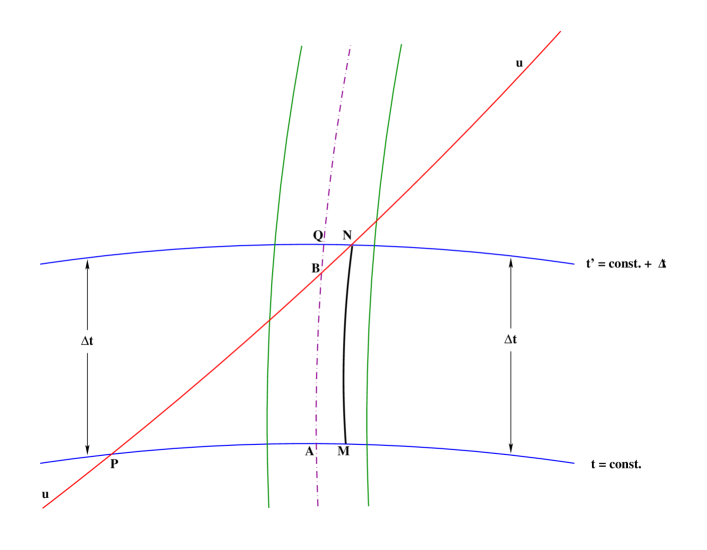
Matching the local and global coordinates requires to calculate integrals of various functions depending on the internal structure of body over two different hypersurfaces of constant time, and , as shown in Fig. 3. Relationship between the integrals taken on the two hypersurfaces is set up by making use of the Lie transfer from one hypersurfaces to another. The integral curves used in the Lie transfer are the world lines of the four-velocity of body’s matter. Only one of such lines, MN, is shown in the figure. Dashed line is the world line of the origin of the local coordinates which coincides with the center of mass of the body under consideration. The center of mass is not associated with four-velocity of body’s matter.
Let us assume that the field point , at which matching of the internal and external solutions of the metric tensor and the scalar field is done, has global coordinates and local coordinates (see Fig. 4). These coordinates are related by the pointwise transformation given by Eqs. (7.2.1) – (7.2.2). By definition, the matching point belongs simultaneously both to the hypersurface of constant time and to that of the constant time . Let us consider a matter element of the central body B located at the point and lying on the same hypersurface of the constant time inside of the body’s world tube. We assume that the point has local coordinates, , and global coordinates, . We emphasize that the time coordinate of the points and is the same because they are located on the same hypersurface of the constant time . However, the time coordinate of the point is different from the time coordinate of the point , that is , because the hypersurfaces of the constant global time passing through the points and are different. Let us consider a world line of the element of the body’s matter passing through the point and intersecting a hypersurface of the constant time at the point . This world line allows us to map coordinates of the element of the body’s matter from the hypersurface to the hypersurface . By the construction, the point must have the global coordinates .
One can expand the spatial coordinates of the world line of the chosen element of the body’s matter in a Taylor series with respect to time
| (8.3.1) |
where is the spatial velocity of the body’s element at the point and . One denotes by letters and position of the origin of the local coordinates on two hypersurfaces, and , respectively (see Fig. 4). Global coordinates of the origin of the local coordinates, taken on two different hypersurfaces, are related by equation
| (8.3.2) |
Now we shall find the time interval separating the two hypersurfaces of the constant global coordinate time, and , under condition that the matching point is fixed. At the point the relationship between the local time and the global time according to Eq. (7.2.1), is
| (8.3.3) |
Subtracting Eq. (7.2.1) from Eq. (8.3.3) and accounting for the fact that the space-time interval between points and is small we obtain
| (8.3.4) |
where the point , that is, it belongs to the hypersurface .
Local coordinates of the point are transformed to the global coordinates as follows
| (8.3.5) |
Expanding functions in the right side of Eq. (8.3.5) in the vicinity of the time instant, , and taking into account Eqs. (8.3.1) – (8.3.4) yields
| (8.3.6) |
where , , and .
Transformation (8.3.6) is used for deriving relationship between the absolute values of functions and which enter denominators of all integrands in the integrals defining the internal gravitational potentials. Subtracting Eq. (7.2.2) from Eq. (8.3.6) and taking the absolute value of the difference gives
| (8.3.7) |
where , , and .
We must also perform a Lie transform to find a relationship between the volume elements and taken at the points and respectively. We note that the invariant density introduced in Eq. (3.3.18) has one more remarkable property in addition to Eq. (3.3.19) [58]. Specifically, the Lie derivative of the product of the invariant density and the volume element is zero, which means that
| (8.3.8) |
Locally measurable velocity of the body’s element at the point is defined with respect to the origin of the local coordinate system. It relates to velocity of the same element of the body taken at point in global coordinates by equation:
| (8.3.9) |
which can be derived from Eq. (8.3.6) by direct differentiation with respect to time.
By making use of Eqs. (8.3.7) – (8.3.9) we finally obtain transformations of the internal gravitational potentials from the local to global coordinates. These transformations are given by the following equations
| (8.3.10) | |||||
| (8.3.11) | |||||
| (8.3.12) | |||||
| (8.3.13) | |||||
| (8.3.14) | |||||
| (8.3.15) | |||||
| (8.3.16) |
where the post-Newtonian correction, , to the Newtonian potential, , reads
| (8.3.17) |
This correction is the result of the post-Newtonian coordinate transformation (7.2.1), (7.2.2) and the Lie-transfer of the integrand of the Newtonian gravitational potential from local to global coordinates. Transformation of all other internal gravitational potentials from local to global coordinates does not require to take into account their relativistic corrections as it would exceed the accuracy of the first post-Newtonian approximation which is redundant.
The matching procedure also requires to derive transformation of the second time derivative of the potential in explicit form. This transformation can be directly obtained from the definition of the potential given by Eq. (4.2.10) and the mapping equation (8.3.12). After straightforward calculation one gets
| (8.3.18) |
where and denote partial derivatives of with respect to the global time coordinate and the spatial coordinate respectively.
8.3.2 Transformation of the External Potentials
External potentials in the internal solution for the metric tensor in local coordinates depend on the external multipole moments , , depend only on time and are ‘pinned down’ to the origin of the local coordinates located at the point where the hypersurface of the constant time intersects with the world line of the origin (see Fig 4). On the other hand, all functions entering the left side of matching equations (7.2.3), (7.2.4) are defined on the hypersurface of constant global coordinate time . Hence, before doing the pointwise coordinate transformation of the external potentials we must perform a Lie transfer of the potentials along the world line of the origin of the local coordinates from point to point located on the hypersurface of the constant global coordinate time . Time shift along this world line is determined by Eq. (8.3.4) where one has to associate the point with the origin of the local coordinates, that is , under condition that the matching point is taken the same as defined in previous section. Keeping in mind that the external potentials are scalars with respect to the Lie transport, one obtains
| (8.3.19) |
where overdot means differentiation with respect to time . After making use of Eqs. (7.2.1) and (8.3.4), and accounting that local coordinates of the point are, , while the global coordinates of the point are, , one gets
| (8.3.20) |
Similar formulas are valid for the multipole moments and as well.
Now we can do the pointwise coordinate transformation of the space coordinates given by Eq. (7.2.2). For the STF product of the local coordinates one has:
| (8.3.21) |
where we have used Eq. (7.2.2). After combining Eqs. (8.3.20) – (8.3.21) all together the post-Newtonian transformation of the Newtonian part of the external potential of the internal solution of the metric tensor assumes the following form
This is the most complicated transformation of the external potential that we need. It takes into account the post-Newtonian nature of the PPN coordinate transformation and supplements Eq. (8.3.10) for the internal Newtonian gravitational potential. All other external potentials present in the local metric (6.2.36) – (6.2.38) are transformed without taking into account the post-Newtonian corrections by making use of only the very first term in the right side of Eq. (8.3.21).
8.4 Matching of a Scalar Field
Scalar field is used in the post-Newtonian terms only. For this reason matching of its asymptotic expansions derived in local and global coordinates is quite straightforward. We operate with external and internal solutions of the scalar field given by Eqs. (4.2.1) and (6.2.3), (6.2.4) respectively. Matching equation (7.2.3) reveals that the internal potentials referred to the central body B cancel out in its left and right sides due to Eq. (8.3.10) while the potentials match to the Newtonian potential and its derivatives referred to the external bodies. More specifically, for any number the matching yields
| (8.4.1) |
where the external Newtonian potential is defined in Eq. (8.2.5) and taken at the origin of the local coordinates, that is the point , at the instant of time . Thus, the STF multipole moment of the external scalar field is fully determined as -th spatial derivative of the Newtonian gravitational potential . We remind that the scalar field was normalized to the factor 313131See Eq. (3.3.10) where in accordance with definition of the PPN parameter ., so that physically observed scalar field . It vanishes in the limit of general relativity where the multipole moments play no role.
8.5 Matching of the Metric Tensor
8.5.1 Matching of and in the Newtonian approximation
Newtonian approximation of the matching equation (7.2.4) for component of the metric tensor in its left side yields
| (8.5.1) |
Function is taken from Eq. (7.3.7) while the global and local metric tensors are taken from Eqs. (4.2.2) and (6.2.36) respectively. One finds that after making use of Eq. (8.3.10) the internal gravitational potentials and drop out of the left and right sides of Eq. (8.5.1). Expanding the external gravitational potential in a Taylor series around the origin of the local coordinates, , and equating similar terms with the same power of specifies the matching conditions
| (8.5.2) | |||||
| (8.5.3) | |||||
| (8.5.4) |
Equation (8.5.2) makes it evident that two functions and can not be determined from the matching procedure separately, only their linear combination can be determined. Hence, one of these functions can be chosen arbitrary. The most preferable choice is to take as it was done, for example, in [45, 69, 94]. This choice is also consistent with recommendations of the IAU [14, 15] and it makes component of the local metric tensor equal to at the origin of the local coordinates if gravitational field of the central body (Earth) is neglected. However, if one chooses the rate of the coordinate time can be different from that of the coordinate time because the average value of functions and is not zero for elliptic orbits. Hence, the choice of can be inconvenient for astronomical data reduction programs in the solar system. Therefore, two time scales, and , have been introduced in such a way that their rate at the origin of the local coordinate system is the same 323232See [14, 15, 99, 101] for more detail.. This makes function
| (8.5.5) |
to be a polynomial of time which numerical coefficients are calculated by means of numerical integration of Eq. (8.5.2) over sufficiently long interval of time [99, 101]. Time-rate adjustment coefficients and relate to each other as [99, 101]
| (8.5.6) |
where is a certain astronomical epoch chosen by convention.
In accordance with the interpretation given in [76, 94], function from (8.5.3) must be understood as acceleration measured by accelerometer being rigidly fixed at rest in the origin of the local coordinates under condition that the internal gravitational field of the central body B is neglected. The choice, , (see, e.g., [42, 94]) leads to construction of a freely falling local coordinate frame which origin moves along a geodesic world line in the background space-time manifold defined by the gravitational potentials of all the celestial bodies of the N-body system but the central body B that is located near the origin of the local coordinates. Such choice of , however, disengage the world line of the center of mass of the central body B from that of the origin of the local coordinates (see Fig. 5).
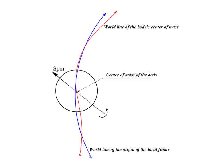
Indeed, the center of mass of the central body (Earth) does not move along the geodesic world line due to the interaction of its internal quadrupole and higher-order multipole moments with the tidal gravitational field of external bodies [45, 47, 58]. For this reason, a special procedure must be applied for finding function which will make the origin of the local coordinates be following the same world line as the body’s center of mass. This procedure is described later in section 9.4 in full details.
STF external multipoles are defined in the Newtonian approximation by Eq. (8.5.4). They describe gravitoelectric [106, 135] tidal gravitational field of external bodies at the origin of the local coordinates. Post-Newtonian corrections to the Newtonian value of the multipoles can be important for lunar laser ranging and other experimental tests of relativistic gravity theory in the near-Earth space. The post-Newtonian corrections to the external multipoles can be also important in construction of the relativistic theory of accretion disc around a star in a close binary system [136]. These corrections are derived later and shown explicitly in Eq. (8.5.4).
8.5.2 Matching of and to the order of
We substitute component of the metric tensor in the global coordinates to the left side of the matching Eq. (7.2.4) and write this equation by taking into account all post-Newtonian terms of order . We find that in this approximation the matching equations reads
| (8.5.7) |
where the matrix of transformation from the local, , to global, , coordinates is given in Eq. (7.3) whereas components of the metric tensor are defined by Eq. (4.2.5) in the global coordinates and by Eq. (6.2.38) in the local coordinates. Comparing similar terms we find that the internal gravitational potentials of the central body B, and , entering the left and right sides of the matching equation, cancel each other and drop out of the matching equation completely. The remaining terms belong to the background gravitational field of external bodies and their matching gives the following set of equations
| (8.5.8) | |||||
| (8.5.9) | |||||
| (8.5.10) | |||||
| (8.5.11) | |||||
| (8.5.12) | |||||
| (8.5.13) |
which define the structure of the PPN transformation between spatial coordinates of the global and local coordinates.
Function defines the unit of measurement of spatial distances in the local coordinates. It would be convenient to chose as it was done, for example, in [45, 94]. However, introduction of TDB and TDT time scales in ephemeris astronomy must be accompanied by the choice of to compensate effects of function from Eq. (8.5.2) on spatial barycentric (global) and geocentric (local) coordinates [101, 102]. In view of this complexity, related to a pure practical application of the PPN theory of reference frames in the solar system, we do not impose any restriction on function at this step of the matching procedure. It will allow us to trace how functions and affect equations of motion of extended bodies.
8.5.3 Matching of and to the order of
Matching equation (7.2.4) for taken in its left side, reads
where we have employed Eqs. (8.5.1) and (8.5.7) for doing simplification. Subsequent substitution of the metric tensor given in the global, Eqs. (4.2.2), (4.2.4) and (4.2.5), and the local, Eqs. (6.2.7) and (6.2.37), coordinates, to Eq. (8.5.3) along with Eqs. (8.2.2) and (8.3.11) for vector-potentials and respectively, reveals that all gravitational potentials depending on the internal structure of the central body B (Earth) cancel each other. Remaining terms in the matching equation (8.5.3) depend only on the background values of the gravitational potentials of external bodies. They yield a number of relationships which allow us to express the external multipole moments from the metric tensor in local coordinates and functions present in the PPN coordinate transformations (7.2.11)–(7.2.14) in terms of the gravitational potentials of external bodies. These relationships are as follows
| (8.5.15) | |||||
| (8.5.16) | |||||
| (8.5.17) |
and
| (8.5.18) | |||||
As one can see the matching equation (8.5.3) gives rise to two sets of equations, Eqs. (8.5.15) – (8.5.17), and Eqs. (8.5.18 – (8.5.3) which have different properties of symmetry. More specifically, Eqs. (8.5.15) – (8.5.17) depend only on objects which are symmetric and trace-free with respect to the entire set of indices . On the other hand, Eqs. (8.5.18), (8.5.3) are symmetric with respect to the set of indices but they are anti-symmetric with respect to any pair of indices consisting of the index and either one off the set . This separation of the matching equation (8.5.3) in the symmetric and antisymmetric components is due to the fact that this equation has one free (vector-type) index and, hence, can be split in fully symmetric and antisymmetric parts in accordance with the Clebsch-Gordan decomposition of the vector spherical harmonics into irreducible representations (see [62, 83, 137] for more details).
Let us now discuss a freedom in choosing angular speed of rotation of spatial axes of the local coordinates. From the discussion in previous sections one knows that there are two possible types of the local coordinates - either dynamically or kinematically non-rotating. Dynamically non-rotating local coordinates are defined by the condition that the external dipole moment in Eq. (6.2.3). On the other hand, the kinematically non-rotating local coordinates are realized if one chooses function in the coordinate transformation, Eq. (7.2.12), for spatial axes. If we do not fix the choice of , then, Eq. (8.5.18) can be rewritten as
| (8.5.20) |
The first term in Eq. (8.5.20) describes the Lense-Thirring gravitomagnetic precession, the second term describes the de Sitter precession, and the third term describes the Thomas precession [20, 57, 76]. We emphasize that in the scalar-tensor theory both the Lense-Thirring and the de Sitter precessions depend on the PPN parameter while the Thomas precession does not. The reason is that the Thomas precession is a special relativistic effect [76] and, as such can not depend at all on a particular choice of a specific gravitational theory. If function , spatial axes of the local coordinates are kinematically rotating. On the other hand, the choice gives kinematically non-rotating local coordinate frame which spatial axes are fixed with respect to distant quasars with neglected proper motions [81].
Functions enter the PPN time coordinate transformation 333333See Eq. (7.2.13). and depend on the gauge-dependent multipole moments which can be chosen arbitrary. There are two of the most preferable options:
-
1)
One simplifies the time transformation, Eq. (7.2.11), from the local coordinates to the global ones as much as possible. In this case the moments have to be chosen such that functions in the time transformation assume the most simple form
(8.5.21) (8.5.22) Here the choice of in Eq. (8.5.21) eliminates all terms explicitly depending on the velocity of the origin of the local coordinates . Substituting Eqs. (8.5.21) and (8.5.22) into Eqs. (8.5.16) and (8.5.17) yields
(8.5.23) This makes the metric tensor and the scalar field in the local coordinates to be determined by four sets of the independent external multipoles , , , and . However, the multipole moments are not physically significant and describe gauge-dependent coordinate effects.
-
2)
One removes from the metric tensor in the local coordinates all physically insignificant multipole moments . The cost of this choice is a more complicated form of the time transformation, Eq. (7.2.11), from the local to global coordinates that involves now the infinite number of coefficients . Assuming that all for one obtains from Eqs. (8.5.16) and (8.5.17)
(8.5.24) (8.5.25)
At the present step of the matching procedure we prefer to keep the multipole moments unspecified to preserve some freedom in making the gauge transformations.
8.5.4 Matching of and to the order of
Matching of the metric tensor at the post-Newtonian order of allows us to infer the post-Newtonian equations of motion of the origin of the local coordinate system as well as the post-Newtonian corrections to the external multipole moments and the remaining part of the time transformation formula (7.2.13) between the local and global coordinates. Expansion of the matching equation (7.2.4) for the metric tensor component, , to the post-Newtonian order, generalizes Eq. (8.5.1)
where the gravitational potentials in the right side of this equations are determined by Eqs. (4.2.2) – (4.2.5) and those in the left side are given by Eqs. (6.2.5), (6.2.6), (6.2.36), (6.2.39) and (6.2.40). Solution of Eq. (8.5.4) is done in several steps.
First of all, one substitutes components of the matrix of the PPN coordinate transformation, given by Eqs. (7.3.7) – (7.3), to Eq. (8.5.4). Then, one matches separately the internal gravitational potentials referred to the central body B and those referred to the external bodies. The internal gravitational potentials have to be transformed from the local to global coordinates by making use of Eqs. (8.3.10) – (8.3.18). One notices that transformation equation (8.3.17) for the Newtonian gravitational potential of the central body B can be written explicitly in terms of the functions coming about the matching procedure at lowest orders. Taking definitions of functions and from section 7.2 and elaborating them by making use of the results of previous steps of the matching procedure, one obtains explicit form of the relativistic correction, , from Eq. (8.3.17) which describes transformation of the Newtonian potential from the local to global coordinates. It reads
Employing this formula in the matching procedure of the internal Newtonian potential of the central body B along with transformation equations for other internal potentials, one gets a remarkable result – both the Newtonian and the post-Newtonian terms depending on the internal structure of the body B cancel out and, hence, completely vanish from the matching equation (8.5.4). This effacing-internal structure effect can be explained in terms of the laws of conservation of intrinsic linear and angular momenta of the body B which are valid in the scalar-tensor theory of gravity as well as in general relativity [20, 65]. In other words, the presence of a scalar field in the scalar-tensor theory of gravity does not result in the net self-force or self-torque exerted on the body which existence would violate classic Newton’s laws. The internal-structure effacing principle for spherically-symmetric extended bodies was extrapolated to the 2.5 post-Newtonian approximation by one of the authors of the present paper [107, 138] by applying the Fock-Papapetrou [48, 49] method for derivation of relativistic equations of motion for a binary system with the conservative and gravitational radiation-reaction forces. Validity of the effacing principle was also confirmed by Damour [79] who derived equations of motion of two Schwarzschild black holes in the 2.5 post-Newtonian approximations by the Einstein-Infeld-Hoffmann technique [139] supplemented by the method of analytic continuation of the energy-momentum tensor of point-like particles understood in terms of the generalized functions (distributions) [137].
At the third step, one equates in Eq. (8.5.4) gravitational potentials generated by all external bodies (Moon, Sun, etc.) but the central body B (Earth). This step requires to know how function, , is transformed from the local to global coordinates within the post-Newtonian accuracy. General formula of transformation of this function is given by Eq. (8.3.2). Substituting to this formula the explicit form of functions and displayed in Eqs. (7.2.6), (7.2.11) – (7.2.14), one gets
Matching equation (8.5.4) requires to calculate function generated by the external bodies other than the body B (Earth) and entering component of the metric tensor in the global coordinates as shown in Eqs. (4.2.3) and (8.2.3). Contrary to other potentials, like , which are solutions of the homogeneous Laplace equation in the vicinity of the body B, function is subject to the Poisson equation [48]
| (8.5.29) |
After solving this equation and expanding its solution into STF harmonics (see appendix A) one obtains
| (8.5.30) |
Differentiating the left and right sides of Eq. (8.5.30) two times with respect to the global coordinate time, , yields
Finally, one expands all functions in both sides of Eq. (8.5.4) in the Taylor series with respect to the distance, , from the central body B, and reduce all similar terms. One finds that those terms which do not depend on (that is, functions of time, , only) form an ordinary differential equation of a first order for function in the coordinate time transformation given by Eq. (7.2.11). This differential equation reads
Terms which are linear with respect to give us the post-Newtonian equation of translational motion of the origin of the local coordinates, , in global (barycentric) coordinates. It generalizes equation (8.5.3) derived solely in the Newtonian approximation. Barycentric acceleration of the origin of the local coordinates with respect to the barycenter of the N-body system is
This equation contains the external dipole moment, , which must be calculated with the post-Newtonian accuracy in order to complete derivation of the post-Newtonian equation of translational motion of the origin of the local coordinates. A simple choice of does not allow us to keep the origin of the local coordinates at the center of mass of the central body B (Earth) for arbitrary long interval of time. This is because the body is, in general, interacting with tidal gravitational field of external bodies (Moon, Sun, etc.) and does not move along a geodesic world line while the choice of makes the origin of the local coordinates moving along a geodesic world line [45, 69, 94]. Thus, function must be defined in such a way that the body’s center of mass and the origin of the local coordinates coincide at any instant of time. This problem is equivalent to solution of the problem of motion of the body’s center of mass with respect to the origin of the local coordinates and will be discussed in the next section.
Terms which are quadratic, cubic, etc., with respect to the distance,, determine the post-Newtonian corrections to the external STF multipole moments , where the Newtonian-like term is shown in equation (8.5.4). The post-Newtonian corrections are
where we used notations
| (8.5.35) | |||||
| (8.5.36) |
These equations finalize description of the STF multipole moments entering external solution of the metric tensor in local coordinates and the parametrized post-Newtonian transformation between the local and global coordinates.
8.6 Final Form of the PPN Coordinate Transformation from Local to Global Coordinates
For the sake of convenience we summarize the final form of the parametrized post-Newtonian coordinate transformation from local to global coordinates which is given by two equations:
| (8.6.2) |
Here functions and are solutions of the ordinary differential equations
| (8.6.3) | |||||
while the other functions are defined as follows
| (8.6.5) | |||||
| (8.6.6) | |||||
| (8.6.7) | |||||
| (8.6.8) |
These equations will be used in subsequent sections for derivation of equations of motion of extended bodies. They are also convenient for comparison with the relativistic transformations derived by other researchers [1, 15, 43, 44, 45, 61, 69, 70].
9 Translational Equations of Motion of Extended Bodies
9.1 Introduction
In the Newtonian theory of gravity definitions of mass and the center of mass of an extended body, which is a member of a many-body system, are quite simple and straightforward concepts. Because of the simplicity, they have been directly extrapolated without any change to the relativistic theory of gravity by Fock [48] by making use of the invariant density which obeys the Newtonian-like equation of continuity, Eq. (3.3.19). The invariant density is defined as mass of baryons per unit of the proper volume and after integration over volume of a body gives its total baryon mass which is constant [20]. The invariant density is used to introduce newtonian definitions of the body’s center of mass, and its linear momentum in the body’s local coordinates. The baryon mass, center of mass and the linear momentum of body B are given 343434We skip in this section label B for all quantities referred to body B as it does not cause misinterpretation. We shall label the bodies with indices A,B,C, etc. every time when it may cause confusion. by integrals [48, 127]
| (9.1.1) | |||||
| (9.1.2) | |||||
| (9.1.3) |
These definitions were used by Fock [48], Papapetrou [49], Petrova [140], Brumberg [131], and some other researchers (see, e.g., [128, 129, 141, 142] and references therein) for derivation of the post-Newtonian equations of translational motion of extended, spherically-symmetric bodies. Physical intuition tells us that equations of motion of such bodies, in principle, have to depend only on masses of the bodies which are supposed to be the only parameters characterizing the magnitude of their internal gravitational field. This is indeed true in the Newtonian theory. It was found, however, that the post-Newtonian equations of motion of spherically-symmetric bodies, unlike the Newtonian theory, depend not only on the baryon masses of the bodies, Eq. (9.1.1), but also on some other characteristics which are the internal kinetic and gravitational energy, elastic energy and moments of inertia [48, 127, 128, 129, 131, 141, 142, 152]. Appearance of such terms significantly complicates interpretation of the post-Newtonian equations of motion and is unsatisfactory from the physical point of view. For instance, due to the dependence of the post-Newtonian equations of motion on other parameters rather than masses of the bodies, it is possible to argue that motion of a binary system consisting of ordinary stars is different from that of a binary system consisting of black holes having the same value of the mass as the stars.
This point of view is incompatible with the Newtonian equations of motion of two black holes as it was shown by Demiansky and Grishchuk [125] who proved that motion of black holes in the Newtonian approximation obeys to the same laws of gravitational physics as for ordinary spherically-symmetric stars. In addition, the Einstein-Infeld-Hoffmann method of derivation of the post-Newtonian equations of motion operates with vacuum Einstein’s equations and does not admit appearance of any terms in the equations of motion of spherical bodies which would depend on the internal structure of the bodies. Thus, one has to expect that the Newtonian definitions of mass, the dipole moment, and the center of mass given in Eqs. (9.1.1) – (9.1.3) are not quite appropriate for calculation of the post-Newtonian equations of motion of extended bodies. Indeed, our study of relativistic translational motion of two spherically-symmetric compact stars in a binary system [107, 108] revealed that if the Newtonian mass and the center of mass are replaced with their corresponding relativistic definitions all terms in the equations of motion depending on the internal structure of the bodies are effectively eliminated via renormalization of masses. Damour [79] called this property ”the effacing principle” and confirmed its validity for spherically-symmetric and compact relativistic bodies using the matched asymptotic expansion technique.
Newtonian theory predicts that if celestial bodies are not spherically-symmetric and rotate, their equations of motion must depend on additional parameters which are the mass multipole moments of the bodies. It is natural to expect that the post-Newtonian equations of motion of such bodies will contain both the mass and current multipole moments given, for example, by Eqs. (6.3) and (6.3.8) respectively. However, it is not evident whether some other parameters have to appear in the relativistic equations of motion in addition to these two sets of the internal multipoles. Scrutiny analysis of this problem in general relativity elucidated that the post-Newtonian equations of motion of extended bodies do contain only the mass and current multipoles [69, 70, 71] and does not depend on any other internal characteristic of the bodies. PPN formalism operates with a class of alternative theories of gravity and does not obey to the ”effacing principle” even for spherically-symmetric bodies because of the violation of the strong principle of equivalence [20, 38, 143, 144]. This violation makes two masses – inertial and gravitational – be different and, hence, two parameters appear in the post-Newtonian equations of motion of spherical bodies as contrasted to general relativistic case. It is interesting to answer the question how many parameters have to be introduced to characterize motion of extended, non-spherically symmetric and rotating bodies in the PPN formalism, thus, extending general relativistic results of Damour, Soffel, and Xu [69, 70, 71].
Like in general relativity, solution of this problem in the PPN formalism could not be achieved in the framework of a standard a la Fock-Papapetrou post-Newtonian approach which basically operates with a single (global) coordinate system. The global coordinates can not be used to define multipole moments of each body in N-body system in a physically consistent way. A local coordinate system should be constructed around each of the bodies in order to strongly suppress coordinate-dependent contributions to definitions of the multipole moments caused by the Lorentz contraction and presence of the background gravitational field caused by external bodies. Consistent relativistic concept of the local coordinate system was developed in [45, 61, 69, 106]. The concept of a local frame of reference associated with a moving body has been also discussed in papers [41, 42, 43, 44]. However, the authors of these papers always assumed that the center of mass of the body moves along a geodesic world line in the background space-time. This assumption is not valid for a non-spherical and rotating body as it follows from the Mathisson-Papapetrou-Dixon equations [49, 75] and other arguments present in [45, 69]. For this reason, the method of construction of the local coordinates in the vicinity of a self-gravitating body suggested in [42, 43] is not general enough. Thorne [62], Blanchet and Damour [63] invented a post-Newtonian definition of the STF mass multipole moments which were fruitfully employed by Damour, Soffel and Xu [69, 70] for derivation of the post-Newtonian translational equations of motion of self-gravitating extended bodies in general relativity. These authors had also proved that the only parameters present in the equations are Tolman masses of the bodies and their STF multipole moments referred to the local frame of reference of each body.
In this section we derive the parametrized post-Newtonian equations of translational motion of extended bodies in the scalar-tensor theory of gravity and prove that these equations depend only on the inertial and gravitational masses of the bodies and a set of STF active multipole moments defined in section 6.3. In case of spherically-symmetric bodies the only parameters present in the equations are the inertial and gravitational masses which are different due to the Nordtvedt effect [143, 144].
Post-Newtonian Thorne-Blanchet-Damour definition of the conserved mass and center of mass of a single isolated body are given by Eqs. (5.5.9) and (5.5.10). One might think that if the body is, in fact, a member of N-body system its gravitational interaction with other bodies of the system would violate these conservation laws [94]. The law of conservation of mass is indeed violated if the body is not spherically-symmetric (see below). However, the law of conservation of the center of mass and linear momentum of the body can be retained.
There are three types of multipole moments in the scalar-tensor theory – active, conformal and scalar – which can be used for definition of body’s mass and its center of mass. These moments were introduced in section 6.3 and are defined by equations (5.2.14), (5.3.6) and (5.4). By direct calculation we shall demonstrate that the active and scalar dipole moments of the body are not efficient in derivation of the translational equations of motion. This is because if one uses either active or scalar dipole and derive equations of motion of the body in its local coordinates the equations, we shall obtain, will contain a significant number of terms which can be treated as self-accelerations and they can not be removed by simple translation of the origin of the local coordinate system to another point. Self-accelerated terms in the equations of motion violate Newton’s third law and are unacceptable. On the other hand, when we use the conformal dipole moment for defining the body’s center of mass and, then, derive equations of motion of the body, we find that self-acceleration terms do not appear, and the equations have remarkably simple structure of the post-Newtonian force which is a function of the active multipole moments of the body coupled with external multipoles.
Let us discuss derivation and specific of the translational equations of motion in more detail starting from the explicit form of the local (macroscopic) equations of motion of the body’s matter in local coordinates.
9.2 Macroscopic post-Newtonian Equations of Motion
The macroscopic post-Newtonian equations of motion of matter consist of three groups: (1) the equation of continuity, (2) the thermodynamic equation relating the elastic energy and the stress tensor , and (3) the Euler equation.
The equation of continuity in the local coordinates has the most simple form for the invariant density and reads
| (9.2.1) |
This equation is exact, that is takes into account all post-Newtonian corrections, as follows from the definition of the invariant density and Eq. (3.3.19).
The thermodynamic equation relating the internal elastic energy and the stress tensor is required only in a linearized approximation where the stress tensor is completely characterized by its spatial components . Hence, one has from Eq. (3.2.5) the following differential equation
| (9.2.2) |
where the operator of convective time derivative is .
The Euler equation 353535In fact, this is the Navier-Stokes equation because the stress tensor is taken in its the most general form. follows from the spatial part of the law of conservation of the energy-momentum tensor . It yields
| (9.2.3) | |||
where gravitational potentials , , , are the metric tensor components in the local coordinates and they have been defined in section 6.2.
9.3 Definitions of Mass, the Center of Mass and the Linear Momentum of an Extended Body in the N-body System
There are two algebraically independent definitions of the post-Newtonian mass in the scalar-tensor theory – the active mass and the conformal mass which are derived from Eqs. (6.3) and (6.3) respectively for index . As discussed in section 6.3 one must retain contribution of the gravitational potential of external bodies in the definition of the STF multipole moments of the body’s gravitational field. It will allow us to cancel out in equations of motion all terms depending on the internal structure of the central body B which are not incorporated to the definition of the STF multipoles. Absence of such terms in equations of motion extends validity of the effacing principle from general theory of relativity [69, 79, 107] to the scalar-tensor theory of gravity at least in the first post-Newtonian approximation. The question about whether to keep the contribution of the gravitational potentials of external bodies in the definition of the STF multipolar decomposition of the body’s gravitational field was discussed by Thorne and Hartle [94] but they did not come up with a definite answer. Our approach is based on direct calculation of equations of motion and we have tried various possible definitions of the center of mass and the STF multipoles. After tedious and cumbersome calculations we came to the conclusion that the equations of motion have the most simple form and the minimal set of parameters if we take the conformal definition of mass and the center of mass for each body and include the gravitational potential of external bodies to the definition of the body’s multipole moments
Conformal multipoles are given by Eq. (6.3) and for index can be reduced to simpler form such that the conformal mass of the body located near the origin of the local coordinates is
| (9.3.1) |
In what follows, we will need definition of the active mass of the body as well. It is extracted from Eq. (6.3) when index
where
| (9.3.3) |
is general relativistic definition of the post-Newtonian mass of the body [20] and
| (9.3.4) |
is the second-order rotational moment of inertia of the body.
It is not difficult to derive a relationship between the active and conformal post-Newtonian masses by making use of Eqs. (9.3.1) – (9.3.3). It reads
where in Eq. (9.4) is called the Nordtvedt parameter [20]. Numerical value of this parameter is known with the precision better than 0.02% from the lunar laser ranging experiment [145] which lasts already for more than 30 years.
One can see that in the scalar-tensor theory of gravity the conformal mass of the body differs from its active mass. If the body is completely isolated the difference can be only due to the Nordtvedt effect, that is for , and the time-dependence of the body’s rotational moment of inertia (for example, radial oscillations, etc.). In the case when the presence of external bodies can not be ignored, one has to account for coupling of the external gravitational field multipoles, and , with the internal multipole moments of the body.
It is important to realize that in general case the general relativistic post-Newtonian mass of an individual body is not conserved. Indeed, taking a time derivative of Eq. (9.3.3) and making use of the macroscopic equations of motion of the body’s matter given in Section 9.2, one gets [129]
| (9.3.6) |
where overdot means the time derivative with respect to the local coordinate time . This equation reveals that the general relativistic mass of the body is constant, if and only if, the mass multipole moments of the body do not depend on time and/or there is no external tidal fields, that is . However, one can notice that the conformal and active post-Newtonian masses are not constant in the presence of the tidal field even if the body’s multipole moments are constant. This is because the external multipole moments enter definitions of these masses, Eqs. (9.3.1) and (9.3), explicitly, and in general case of N-body problem they depend on time.
Direct calculation of the equations of motion elucidates that definition of the conformal mass dipole moment given by Eq. (6.3.5) for gives the most optimal choice of the post-Newtonian center of mass for each body. This is because after differentiation with respect to time only the conformal dipole moment leads to the law of conservation of the body’s linear momentum when one neglects the influence of other external bodies, while the post-Newtonian scalar or active dipole moments do not bear such property. Thus, the post-Newtonian center of mass of the body, , is derived from Eq. (6.3.5) for and reads
where here and everywhere else symbol
| (9.3.8) |
denotes a new STF object [1]. We call attention of the reader to the fact that for the scalar function , where has been defined in Eq. (9.3.4).
It is worth noting that the post-Newtonian definitions of mass and of the center of mass of the body depend not only on the internal distribution of matter’s density, velocity, and stresses inside the body but also on terms describing the coupling of body’s gravitational field with that of external masses. As we shall show later, inclusion of these coupling terms in definitions (9.3.1), (9.3) and (9.3) is absolutely necessary in order to simplify translational equations of motion as far as possible and bring them to the form which can be reduced to the Einstein-Infeld-Hoffmann equations of motion in the limiting case of spherically symmetric bodies. In this sense, the question about whether the coupling of internal and external gravitational fields should be included in the definitions of the post-Newtonian mass and the center of mass, which was a matter of concern for Thorne and Hartle [94], can be considered as having been resolved.
The post-Newtonian linear momentum of the body, , is defined as the first time derivative of the dipole moment given by Eq. (9.3), that is , where dot indicates a derivative with respect to the local coordinate time . After taking the derivative one obtains
where function
| (9.3.10) |
Until now the point represented location of the origin of the local coordinate system in the global coordinates taken at the time . In general, the origin of the local coordinates does not coincide with the center of mass of the body which can move with respect to the local coordinates with some velocity and acceleration. In order to be able to keep the center of mass of the body at the origin of the local coordinates one must prove that for any instant of time the dipole moment defined by Eq. (9.3) and its time derivative (that is, the linear momentum of the body) given by Eq. (9.3) can be made equal to zero. This requirement can be achieved, if and only if, the second time derivative of the dipole moment with respect to the local coordinate time is identically equal to zero, that is
| (9.3.11) |
It is remarkable that this equation can be satisfied after making an appropriate choice of the external dipole moment that characterizes a locally measurable acceleration of the origin of the local coordinates with respect to another local coordinate frame whose origin moves along a geodesic world line in the background space-time. This statement has been proven in [45] in the Newtonian approximation and, then, extended up to the first general relativistic post-Newtonian approximation in [69]. In the present paper we shall derive the consequences of Eq. (9.3.11) in the first post-Newtonian approximation of the scalar-tensor theory of gravity characterized by two PPN parameters, and .
9.4 Translational Equation of Motion in Local Coordinates
Translational equation of motion of the body in the local coordinates, , is derived by making use of the definition of its conformal linear momentum, , displayed in Eq. (9.3). Differentiating Eq. (9.3) one time with respect to the local coordinate time , operating with the macroscopic equations of motion, Eqs. (9.2.1) – (9.2.3), and integrating by parts to re-arrange some terms, one obtains
where we have shown explicitly all terms proportional to , , and the post-Newtonian correction is given by
It is worth noticing that mass is the active mass, and the STF multipole moments () of the body, which appear in the right side of Eqs. (9.4) and (9.4), are the active mass multipole moments depending on time . Function in Eq. (9.4) has not been yet restricted and can be chosen arbitrary. Its choice determines a world line of the origin of the local coordinates. If one chooses , then the origin of the local frame, , is moving along a geodesic world line defined in the global frame by Eq. (8.5.4) and the center of mass of the body under consideration is moving in accordance with the law of motion, Eq. (9.4), with respect to this geodesic. For practical applications, however, it is more convenient to chose the origin of the local frame to be always located at the center of mass of the body. This can be accomplished by imposing condition (9.3.11), that is . If this condition is satisfied it allows us to chose exactly, which leads to similar conditions for the active dipole moment, , in the Newtonian approximation. However, in the post-Newtonian approximation the active dipole moment of the body, , even if the conformal multipole moment of the body, , because these two moments are defined via different equations (see Section 6.3).
Fixing the origin of the local frame at the body’s center of mass () and noticing that for any makes the post-Newtonian function . Then, one can find solution of Eq. (9.4) for function which was considered until now as arbitrary variable. We remind that the physical meaning of is acceleration of the origin of the local coordinates with respect to a geodesic world line in the background space-time defined by the gravitational field of external bodies. Equating , separating acceleration of the body’s center of mass from all other terms in Eq.(9.4) and taking all terms with to the right side yields the following post-Newtonian equation
| (9.4.3) |
where the conformal anisotropic tensor of mass
| (9.4.4) |
and the (tidal) gravitational forces
| (9.4.5) | |||||
Eqs. (9.4.3) – (9.4) describe the law of translational motion of the body in the local coordinates in the presence of external bodies which create a force dragging motion of the body’s center of mass from geodesic world line. Newtonian, , and the post-Newtonian, , tidal forces are caused by gravitational coupling of the body’s internal (active) multipole moments, and , with the external multipole moments, and . The post-Newtonian tidal force, , is reduced in the limit of to general relativistic expression derived previously by Damour, Soffel and Xu [69].
It is worthwhile to emphasize that summation with respect to index in Eq. (9.4.5) begins from . The point is that we have defined the center of mass of the body in terms of the conformal dipole moment by the condition . However, the force depends on the active multipole moments of the body but the active dipole moment and, hence . For this reason, one has to take into account the contribution to the force coming out of the non-zero active dipole of the body. This contribution has a post-Newtonian order of magnitude and can be written down in more explicit form as
| (9.4.8) |
where the active dipole moment is 363636We remind that the conformal dipole moment of the body, . Hence, Eq. (9.4.8) is, in fact, a difference between the active and conformal dipole moments of the body, .
where
| (9.4.10) |
If one takes into account explicit relationships between the multipole moments of the scalar field and gravitational potential of the external bodies, then Eq. (9.4) can be slightly simplified
It is clear that dipole moment of the central body can contribute to the equations of motion of the body only in the scalar-tensor theory of gravity because in general relativity . It is important to notice the presence of the Nordtvedt parameter in the active dipole moment of the body. It is likely that we observe a general feature of the relativistic equations of motion in the scalar-tensor theory. It looks like each active multipole moment of the body under consideration has a contribution being proportional to the Nordtvedt parameter . This, for example, leads to inequality between inertial and gravitational masses of the body in case of the monopole mass moment. Presence of the Nordtvedt parameter-dependent term(s) in dipole moment is insignificant for the bodies whose shape is close to spherically-symmetric. However, it may play a role in motion of sub-systems, like that of Earth and Moon, which possess large deviations from spherical symmetry. Experimental study of this problem would be desirable.
Gravitational force is also essential only in the scalar-tensor theory of gravity. It is proportional to the dipole moment of the scalar field and its time derivatives. Had the scalar field absent the dipole moment of the scalar field could not exist and the force would be zero. The dipole moment of the scalar field couples with the self-gravitational energy of the body as well as with the energy of external gravitational field and kinetic energy of the body’s internal motion 373737Observe the term . In the next section we shall show that it is this coupling that is responsible for inequality of inertial and gravitational masses of the body and should be treated as a violation of the strong principle of equivalence.
9.5 Equation of Translational Motion in Global Coordinates
Equation of translational motion of the body’s center of mass in the global coordinates can be obtained from the equation of motion, Eq. (8.5.4), of the origin of the local coordinates, , if the acceleration is subject to obey to the local equation of motion. (9.4.3). The acceleration depends on scalar multipoles so that after substitution Eq. (9.4.3) to Eq. (8.5.4) one has to make use of Eq. (8.4.1), that is . Moreover, one has to use Eq. (8.5.3) to replace in forces , , and all terms depending explicitly on with a linear combination of the barycentric acceleration and the gradient of the gravitational potential of external bodies, . Taking all terms depending on the gravitational gradient to the right side of Eq. (8.5.4) and those depending on the barycentric acceleration to the left side, bring Eq. (8.5.4) to the following form
where the external potentials , , , and are defined in Eq. (8.2.5) and are taken on the world line of the center of mass of the body B. The external potentials can be expanded in multipolar series so that the translational equation of motion (9.5) will depend only on the active multipole moments of the bodies. We do not present this general result in the present paper but consider a more simple case of spherically-symmetric and rotating bodies in section 11.
One has to notice that inertial mass of the body B is its conformal mass. It is not equal to gravitational mass of the body in the right side of this equation which is its active mass. Difference between the two masses is given by Eq. (9.3) and it causes violation of the strong principle of equivalence for massive extended bodies. Existence of the possible difference between the inertial and gravitational masses in alternative theories of gravity was pointed out by Dicke [36, 37, 38] and Nordtvedt [16, 17, 145]. In our calculations the inertial-gravitational mass difference originates from Eq. (9.4) which has terms proportional to scalar dipole, , and they contribute to the gravitational (active) mass only.
Forces and are given by Eqs. (9.4.5) and (9.4.6). Terms in the first and second curled brackets of Eq. (9.5) being proportional to mass are the post-Newtonian corrections to the Newtonian force acting on the body B considered as a monopole massive particle . The group of terms in third and forth curled brackets in Eq. (9.5) represents the post-Newtonian correction to the Newtonian tidal force and takes into account higher order multipoles of the body B. In particular, these terms contain time-dependent functions and which define the unit of time and length in the local coordinates. This correction also contains the matrix of relativistic precession given in Eq. (8.6.8). Eq. (9.5) describes a generic case of translational equation of motion of extended bodies having arbitrary shape and rotation (all multipoles). We derive rotational equation of motion of the body B in the next section.
10 Rotational Equations of Motion of Extended Bodies
Rotational equations of motion for each body define orientation of the body’s angular momentum (spin) at each instant of time with respect to the local frame of reference which axes are not dynamically-rotating, that is Fermi-Walker transported [76] in accordance with Eq. (8.6.8) describing orientation of the axes of the local coordinates with respect to the global coordinates at each instant of time. We shall work out relativistic equations of the rotational motion by making use of the method proposed in [71].
10.1 Post-Newtonian Definition of the Angular Momentum of the Body
First of all, one needs to introduce definition of the angular momentum of an extended body from the N-body system. In principle, one had to use the same principle of the multipolar expansion of the metric tensor applied to its component calculated with taking into account all terms of the next post-Newtonian approximation. This procedure was applied by Damour and Iyer [64, 91] for the post-Newtonian definition of angular momentum of an isolated system. It is not known yet how to apply the Damour-Iyer procedure to a single body from the N-body system because of its complexity. Therefore, we shall use the approach proposed in [71] to bypass this difficulty.
Let us introduce a bare spin of a single body B by making use of the following post-Newtonian definition
| (10.1.1) |
where
| (10.1.2) |
is a linear combination of tensor of energy-momentum of matter and the pseudo-tensor of gravitational field . We have defined the bare spin of the body B by Eq. (10.1.1) because it corresponds to the conserved spin of an isolated system (see Eq. 5.5.6 for more detail). We also assume that the center of mass of the body B is chosen such that its conformal dipole moment is zero.
Integration in Eq. (10.1.1) is formally performed in local coordinates over entire space. However, tensor of energy-momentum includes the matter of the body B only and depends on the complete metric tensor in the local coordinates. We assume that the pseudo-tensor depends only on the internal part of the local metric tensor for the body B. Integration by parts allows us to reduce the bare spin of the body B in Eq. (10.1.1) to the following expression
where integration is over the volume of the body B, and potential is defined by Eq. (9.3.10). We shall use Eq. (10.1) to derive rotational equations of motion of body’s angular momentum.
10.2 Equations of Rotational Motion in Local Coordinates
Rotational equations of motion for body’s spin are derived by differentiation of Eq. (10.1) with respect to the local coordinate time . After taking the time derivative and making use of the macroscopic equations of motion in local coordinates given in section 9.2, one makes several transformations of the integrand to reduce similar terms and to simplify final result. After tedious but straightforward calculations done in the spirit of paper [71], one obtains equations of the rotational motion of body B in its own local coordinate frame
| (10.2.1) |
where is a general-relativistic torque for , and is its post-Newtonian correction due to the presence of the scalar field, while can be considered as a supplementary post-Newtonian contribution to the bare spin . The torque and other terms in the right side of Eq. (10.2.1) read as follows:
| (10.2.2) | |||||
where
| (10.2.5) |
is additional set of multipole moments which has been used already in definition of the multipole moments in section 5.
General relativistic torque depends on the multipole moments which define the residual gauge freedom. They can be used to simplify the post-Newtonian correction to the torque, . This correction is, in fact, exactly equivalent to , where and are active and conformal dipole moments of the body B respectively. The difference between the two dipole moments taken under condition that is given by Eq. (9.4) and has been reproduced in Eq. (10.2). We have taken into account the external monopole moments and defining the units of measurement of the local time and spatial coordinates respectively. Their contribution is to the rotational equations of motion is extremely small and can be omitted.
We re-define the spin of the body as
| (10.2.6) |
so that equations of rotational motion acquire their final form
| (10.2.7) |
These equations should be compared with analogous equations derived by Klioner and Soffel [1] 383838These equations are numbered (9.42) – (9.47) in [1]. First of all, we notice that our definition of the multipole moments differs by a numerical factor from that, , used by Klioner and Soffel, that is
| (10.2.8) |
Comparison of spins, – our notations, and, – Klioner-Soffel’s notation, shows that they are equal if sign minus in front of three last terms in Eq. (9.45) of Klioner-Soffel’s paper [1], is replaced with sign plus. The general relativistic torque in the present paper coincides naturally with that derived in [1]. The biggest difference occurs between the post-Newtonian correction to the torque in this paper and a corresponding quantity given in two equations, (9.43) and (9.46), in the paper [1]. First three terms in our Eq. (10.2) completely coincides with equation (9.43) derived by Klioner and Soffel, thus, confirming the presence of the Nordtvedt effect for rotational motion of the bodies. However, we obtained different terms in the second and third lines of our Eq. (10.2) as contrasted with equation (9.46) of Klioner and Soffel’s paper [1]. We suppose that the difference may come out of slightly different gauge conditions used in this paper and in [1]. Additional origin of the difference is that we used definition of the center of mass of the body which is not reduced to that used by Klioner and Soffel.
11 Motion of spherically-symmetric and rigidly-rotating bodies
11.1 Definition of spherically-symmetric and rigidly rotating body
It is well understood that the notion of a spherically-symmetric and rigidly rotating body is not invariant but coordinate-dependent [66, 76]. According to special theory of relativity, coordinate grid of a moving coordinate frame is linearly deformed and magnitude of this deformation depends on velocity of the frame with respect to a reference frame being at rest. This consideration assumes that if one considers a spherically-symmetric body in a static frame it will be not spherically-symmetric in a moving frame. Deformation of the body’s shape can be calculated by applying the Lorentz transformation to the equation describing the shape of the body in the static frame [146]. The Lorentz deformation is solely coordinate effect which does not lead to appearance of physical stresses (tensions) inside the moving body. Nonetheless, the Lorentz deformation of the body’s shape has to be taken into account for correct calculation of observed physical effects associated with motion of the body. Poincaré and Lorentz were first who took into account special relativistic deformation of a moving electron for calculation of the electromagnetic radiation-reaction force exerted on the electron due to the emission of electromagnetic radiation [147].
In general relativity gravitational field causes deformation of coordinate grid of a static frame with respect to the grid of the same frame taken in the absence of gravitational field 393939This represents pure mathematical comparison. It is not physically possible to turn off or to screen gravitational field.. Hence, this distortion of the coordinate grid represent pure mathematical effect and does not cause physical deformation of the body being at rest with respect to this frame. However, gravity-caused deformations of the local coordinate’s grid must be taken into account in calculation of translational equations of motion of the body with respect to the global coordinate frame. It is worth mentioning that one has to distinguish the mathematical deformations of the frame from the physical (tidal) deformations of the body itself [72]. This can be achieved if a precise relativistic theory of reference frames is employed. The PPN formalism brings new complications due to the presence of additional fields which can cause both coordinate and physical deformations of the body’s volume.
Post-Newtonian definition of the multipole moments of the gravitational field is coordinate-dependent. Therefore, the explicit structure of the multipolar expansion and the number of terms present in this expansion crucially depend on the choice of coordinates. Transformation from local coordinates to global ones will change mathematical description of the multipole moments and we have to be careful in finding the most precise formulation of the notion of spherically-symmetric body to avoid introduction of non-physical multipole moments. Any misunderstanding of this concept will lead to inconsistencies in calculation of equations of motion for N-body problem in the first [107] and higher-order post-Newtonian approximations [148] and/or appearance of spurious coordinate-dependent terms having no physical meaning.
We assume that for each body of N-body system the geometrical center of the body’s spherical symmetry is located at the center of mass of the body that coincides with the origin of the local coordinates associated with this body. We assume that all functions characterizing internal structure of the body have spherically-symmetric distribution in the local coordinates. These functions are: the invariant density , the internal energy , and the stress tensor . Spherical symmetry in the local coordinates means that these functions depend only on the local radial coordinate :
| (11.1.1) |
Moreover, we assume that the internal distribution of matter does not depend on the local coordinate time that excludes radial oscillations of the body from consideration. Radial oscillations can be easily included in our version of the PPN formalism but we postpone treatment of this problem for future work 404040Notice that radial oscillations are irrelevant for consideration of this problem in general relativity due to the Birkhoff’s theorem [66, 76].
Spherically-symmetric distribution of matter must generate a spherically-symmetric gravitational field. Therefore, the multipolar expansion of the Newtonian gravitational potential of the body must have in the local coordinates only a monopole term
| (11.1.2) |
where the baryon (Newtonian) mass is defined in Eq. (9.1.1). Strictly speaking, this monopole expansion will be violated at some order of approximation because the external tidal force of the background gravitational field acts on the body and deforms its spherically-symmetric distribution of matter. This tidal distortion is proportional to some numerical coefficient 414141Love’s number [68]. which characterizes elastic properties of the body under consideration. Assuming that the body is made of matter with sufficiently low elasticity one can reduce the tidal deformation of the body to a negligibly small value, at least in the first post-Newtonian approximation 424242Analytic estimate of the magnitude of the tidal deformation comparatively with the magnitude of the post-Newtonian forces has been done in [79, 107]..
We shall consider the case of rigidly rotating bodies for which the internal velocity of matter (as defined in the local coordinates) is a vector product of the angular velocity , referred to the local frame, and the radius-vector , that is
| (11.1.3) | |||||
| (11.1.4) |
in the local frame of the body B. Again, one should remind that rotation causes rotational deformation of the body and distorts spherical symmetry. However, the rotational deformation is proportional to the same Love’s number, , [68] and by assuming that the body is rigid enough and rotates sufficiently slow, one can make the rotational deformation to be negligibly small. In what follows we shall use this assumption and neglect the rotational deformation.
Spherical symmetry of each body assumes that one can use the following (pure geometric) properties which are valid for any function , depending on radial coordinate only [62]:
| (11.1.5) | |||||
| (11.1.6) |
where is the fully symmetric linear combination of the Kronecker delta symbols [62]. In particular, for any one has
| (11.1.7) |
One will also need several other equations for performing integration over sphere in the local coordinates of body B. They are as follows:
| (11.1.10) | |||||
| (11.1.13) |
where we used Eq. (11.1.4), and are arbitrary STF tensors, and
| (11.1.14) |
is -th order rotational moment of inertia of the body B 434343Notice that all odd rotational moments ..
11.2 Coordinate Transformation of Multipole Moments
Multipolar expansion of the Newtonian potential in the global coordinates, , introduces multipole moments of a body defined as integrals over the body’s volume taken on hypersurface of constant time , that is
| (11.2.1) |
where , and is the origin of the local coordinates coinciding with the center of mass of the body. We have postulated that the density and other structure-dependent functions inside the body have a spherical-symmetric distribution in the local coordinates , so that according to Eq. (11.1.7) the following relationship must held for any
| (11.2.2) |
where the integration is over a hypersurface of constant local coordinate time . However, Eq. (11.2.2) does not assume that the multipole moments of the body B defined in the global coordinates, , equal zero, in fact for . One can calculate directly from Eq. (11.2.2) after making use of transformation formula, Eq. (8.3.6), from the local to global coordinates 444444This kind of transformation of the multipole moments turns out to be important for calculation of the 3-d post-Newtonian equations of motion [148].
where , , , , and
| (11.2.4) | |||||
| (11.2.5) | |||||
| (11.2.6) |
and function is defined in Eq. (8.5.20).
Eq. (11.2) must be used for transforming integrals shown in Eq. (11.2.2) from the local to global coordinates. This is because the integration in Eq. (11.2.2) is performed over the hypersurface of constant (local) time coordinate while similar integrals in the multipolar decomposition of the Newtonian gravitational potential in the global coordinates are defined on the hypersurface of constant (global) time coordinate . Transformation of space coordinates from the space-like hypersurface of constant time to that of time depends on space coordinates, , of the point at which matching of the local and global coordinates is done so that the two space coordinates: – the point of integration, and, - the matching point, appear in Eq. (11.2) simultaneously and they both belong to the hypersurface of constant time .
Substitution of Eq. (11.2) into Eq. (11.2.2) yields [138]
Taking into account Eq. (11.2.2) one concludes that only the dipole, , and the quadrupole, , moments differ from zero. More specifically, one has
| (11.2.8) | |||||
| (11.2.9) | |||||
| (11.2.10) |
The same expressions for the multipole moments can be obtained in a different way by making use of multipolar expansions of the Newtonian potential of body B in the local and global coordinates and their subsequent comparison with the help of transformation formula shown in Eq. (8.5.4). We have checked that both derivations are self-consistent and yield identical expressions for multipole moments given in Eqs. (11.2.8) – (11.2.10). Transformation of multipole moments of Earth’s gravitational field from the global to local coordinates were used in our papers [60, 61] in order to derive the post-Newtonian equation of motion of Earth’s artificial satellites (valid also for Moon) in the geocentric frame with taking into account relativistic corrections due to the presence of Earth’s quadrupole field.
11.3 Multipolar Decomposition of Gravitational Potentials in Global Coordinates
In order to derive equations of motion of the bodies in global coordinates one will need to know the multipolar decomposition of gravitational potentials , , , and in these coordinates. The potentials under discussion are defined in Eqs. (4.2.8) – (4.2.14). For the Newtonian potential one has
where the dipole, , and quadrupole, , moments are given by Eqs. (11.2.8) and (11.2.9).
Vector-potential is decomposed as follows
| (11.3.2) |
where we have used the fact that inside the body, , and the internal velocity, , is defined in Eq. (11.1.3).
Superpotential has the following multipolar decomposition
| (11.3.3) |
Potential consists of a linear combination of four functions as shown in Eq. (4.2.6). For each of these functions one has
| (11.3.6) | |||||
| (11.3.7) |
This concludes the set of equations describing the multipolar decomposition of the gravitational potentials in the global coordinates.
11.4 Translational Equations of Motion
Both conditions of spherical symmetry and rigid rotation, Eqs. (11.1.1) and (11.1.3), allow us to simplify equation (9.5) of translational motion of body B drastically. For example, Eq. (11.1.7) assumes that all multipole moments of the body for all , and for all . Therefore, calculation of the tidal Newtonian force for body B, taken from Eq. (9.5), yields
| (11.4.1) |
which has the post-Newtonian, (), order of magnitude.
The post-Newtonian gravitomagnetic tidal force from Eq. (9.5) in case of a spherically-symmetric body is reduced to
| (11.4.2) |
where the external (gravitomagnetic-type) quadrupole
is the mass, and
| (11.4.4) |
is the spin of the body B.
All other terms in Eq. (9.5) depending on are equal to zero. Hence, Eq. (9.5) is drastically simplified for spherically-symmetric bodies and reads
where the conformal, , and active, ,masses od the body B are related to each other via Eq. (9.3), that is
| (11.4.6) |
and the gravitational potential
| (11.4.7) |
The tidal force is given by Eq. (11.4.1) and is shown in Eq. (11.4).
We are to calculate all terms in the right side of Eq. (11.4) explicitly in terms of body’s mass, rotational moment of inertia, and spin. Among them the most complicated is the first one, that is . By making use of Eqs. (11.3) – (11.3.7) we obtain
where
| (11.4.9) |
is the active mass of the body C, is the general relativistic mass of the body C defined by Eq. (9.3.3) where for the sake of simplicity we assumed , and is the Nordtvedt parameter.
After calculating derivatives from potentials , and substituting them into Eq. (11.4) one obtains the following expression for acceleration of the center of mass of the body B:
| (11.4.10) |
where is the Newtonian force and , , are the post-Newtonian relativistic corrections. Gravitational forces in the right side of this equation are given by the following expressions
| (11.4.11) | |||||
where we have defined , and spin of body B relates to the angular speed of the body’s rotation via Eq. (11.4.4).
Eq. (11.4.10) elucidates that inertial mass of the body B is simply its general relativistic mass given by Eqs. (9.3.3). This mass is conserved (constant) for spherically-symmetric bodies as follows from Eq. (9.3.6). The Nordtvedt gravitational mass of the body B depends on the gravitational defect of mass multiplied with the Nordtvedt parameter
| (11.4.16) |
The Newtonian gravitational force , Eq. (11.4.11), depends in the scalar-tensor theory only on the Nordtvedt gravitational masses of the bodies. Will [20] distinguishes the ”active” and ”passive” gravitational masses which depend on the entire set of the PPN parameters. In our approach used in the present paper only two PPN parameters, and , exist. In this case the ”active” and ”passive” gravitational masses coincide and reduce to one and the same expression given by Eq. (11.4.16). Inertial and gravitational masses of the body are not equal in the scalar-tensor theory of gravity [38, 143, 144]. This inequality violates the strong principle of equivalence for massive bodies. This violation can be also explained from the point of view of interaction of the gravitational field of the body under consideration with the scalar field generated by external bodies. This interaction leads to a local force which brings about a non-zero value of the time derivative of the body’s linear momentum. Indeed, assuming that the body under consideration has finite size, is non-rotating, and spherically-symmetric, one obtains from Eq. (9.4)
where is a gradient of the scalar field of the external bodies. If one keeps the body’s center of mass at the origin of the local coordinate system (), then, the body’s center of mass will experience an anomalous acceleration . This anomalous acceleration is due to the interaction of the gravitational energy (”gravitational charge”) of the body under consideration with the gradient of the external scalar field. The coupling constant of this interaction is the dimensionless Nordtvedt parameter .
The post-Newtonian forces, Eqs. (11.4)–(11.4), depend only on the general relativistic masses of the bodies which coincide with the Newtonian definition of mass, Eq. (9.1.1) in the approximation under consideration. The post-Newtonian force (11.4) is known as the (Lorentz-Droste) Einstein-Infeld-Hoffmann (EIH) force [149] presently used as a basis of JPL ephemerides [21]. It was derived in general relativity by Lorentz and Droste [150] and later by Einstein, Infeld and Hoffmann [139], Petrova [140], and Fock [48]. In the Brans-Dicke theory this force was derived by Estabrook [151] in case of and by Dallas [152] in the case (see also [153]). These derivations assumed that the bodies have negligible ratio of their radii to the characteristic distance between the bodies (a point-like body approximation) as well as that they are non-rotating and move along geodesic world lines.
Corrections to the EIH force are given by Eqs. (11.4) –(11.4). The force given by Eq. (11.4) describes the relativistic post-Newtonian correction to the EIH force due to the coupling of the body’s spin with orbital angular momentum and rotational spins of other bodies. It depends on the PPN parameter only. If one takes in Eq. (11.4), the force is reduced exactly to its general relativistic expression obtained earlier by other researchers [70, 127, 154, 155]. Our Eq. (11.4) for the PPN force coincides with that derived by Klioner and Soffel [1].
The force (11.4) describes general relativistic correction to the EIH force due to the finite size of the bodies. This correction is proportional to the forth-order rotational moments of inertia of the bodies, , while all terms, which are proportional to the second-order body’s rotational moments of inertia, , cancelled mutually out. Nordtvedt [156] considered the problem of translational motion of extended bodies in the general class of scalar-tensor theories of gravity. He came to the conclusion that covariant formulation of the variational principle requires the second-order moment of inertia of extended body to be coupled with the Ricci tensor of the background gravitational field generated by the external bodies. Hence, such coupling must disappear in general theory of relativity by virtue of the vanishing of the background Ricci tensor in vacuum. However, body’s moments of inertia of higher order couple with the full Riemann tensor and its derivatives, and for this reason they can present in general relativistic equations of motion of spherically-symmetric bodies as demonstrated in Eq. (11.4).
Nordtvedt’s calculation [156] of the equations of motion of extended spherically-symmetric bodies agrees with our derivation of these equations based on the implementation of the matched asymptotic expansion technique and separate solution of the internal and external problems for gravitational field of the N-body system. However, vanishing of all terms depending on the second order rotational moment of inertia in general relativity is in disagreement with calculations of Brumberg [127], Spyrou [128], Dallas [152] and Vincent [153] who came to the conclusion that the general relativistic Lagrangian for the system of N spherically-symmetric bodies must depend on the second-order moments of inertia of these bodies, . Brumberg’s expression for the force due to the finite size of the bodies is [127]
We have analyzed and pinned down the origin of the disagreement between Nordtvedt’s [156] and Brumberg’s calculations. Nordtvedt [156] used covariant approach while Brumberg [127] followed Fock’s method [48] and operated with the coordinate-dependent definitions of the multipole moments. In fact, Brumberg defined multipole moments of the bodies in the global (barycentric) frame of the N-body system. Spherical symmetry of the bodies was also defined by Brumberg in the global frame. Such definition of the spherical symmetry does not comply with the relativistic law of transformation between local and global frames. Hence, the bodies can sustain their spherically-symmetric shape in the global frame if and only if there are internal stresses in the body’s matter which compensate for the Lorentz and gravitational contractions of the body’s shapes [138]. Existence of such coordinate-dependent internal stresses inside the body under consideration is unnatural. Furthermore, assumption about spherical symmetry of the bodies in the global barycentric frame brings about the force which is a pure coordinate effect.
In order to prove that the force has no physical origin we have considered translational equation of motion for body B defined in the global frame as follows
| (11.4.19) |
where the post-Newtonian corrections (not shown explicitly) include the relativistic point-like effects and Brumberg’s force (11.4). Barycentric velocity of the body’s matter is obtained by differentiation with respect to time of both sides of Eq. (11.2) and can be decomposed to the sum of the barycentric velocity of the body’s center of mass, , and the internal velocity’s field in local coordinates
| (11.4.20) |
where is the relativistic correction to the local velocity . This correction is a quadratic function of the local coordinates of the body. Hence, subsequent calculation of the time derivative of and calculation of the integral in the left side of Eq. (11.4.19) bring about terms which actually depend on the moment of inertia of body B. This moment of inertia is reduced to the rotational moment of inertia in case of a spherically-symmetric body. Calculation of the integral from the Newtonian potential in the right side of Eq. (11.4.19) has to be done by splitting the potential in two parts - internal and external (see Eq. (8.2.1)), and applying Eqs. (11.3) and (11.2.8), (11.2.9) for calculation of the integrals from the external potential. This again gives a number of terms depending on the rotational moment of inertia of the body B. Summing up all these terms one obtains exactly the same expression as in Eq. (11.4) but with opposite sign. It means that these terms cancel out with the force . This completely agrees with our calculations of the force which does not depend on the body’s rotational moments of inertia of the second order. We conclude that the origin of the coordinate-dependent force is directly associated with an inappropriate choice of the body’s center of mass and the property of its spherical symmetry which must be defined with respect to the local coordinate frame co-moving with the body under consideration. Brumberg attempted to make more physical calculation of the force in his another book [131] but he did not arrive to any definite conclusion regarding whether the force depends on the body’s rotational moments of inertia of the second order or not. Our calculations resolve the problem and demonstrate that force does not exist 454545In the sense that has no physical impact on the motion of the bodies having finite size. and that general relativistic correction due to the finite size of the moving bodies is proportional to the forth and higher order rotational moments of inertia of the bodies. These corrections are extremely small for the bodies comprising the solar system and can be neglected in treatment of the solar system gravitational experiments. However, finite size effects can become important during the final stage of coalescence of binary neutron stars so that they should be included in the precise calculation of templates of the gravitational waveforms.
The force describes relativistic correction due to the finite size of the bodies in the scalar-tensor theory of gravity. This force is proportional to the parameter only and, in contrast to general relativity, depends on the second order rotational moments of inertia, . This dependence was noticed by Nordtvedt [156, 157] who has found that in the case of weakly self-gravitating bodies the finite-size effects are proportional to . This is in disagreement with our calculations of the force but one can easily reconcile the two formulations. The matter is that Nordtvedt [157] worked in harmonic coordinate system defined by the condition while we worked in the quasi-harmonic coordinates defined by the Nutku condition (see Eq. (3.4.1) in the present paper). This leads to two different forms of the transformation between spatial global and local coordinates. In harmonic coordinates this transformation reads [1, 157]
while in the quasi-harmonic coordinates, used in the present paper, we have
The two transformations have different dependence on in terms proportional to the acceleration so that
| (11.4.23) |
It is due to this difference the parameter had appeared in Nordtvedt’s calculations of the finite size effects and made the parameter characterizing the magnitude of the finite-size effects in the harmonic coordinates. However, dependence of the magnitude of the finite-size effects on the parameter in Nordtvedt’s calculations is a pure coordinate effect which has no physical meaning. Parameter can be eliminated from the force if one works in the quasi-harmonic coordinates defined by the Nutku condition (3.4.1) of this paper.
11.5 Rotational Equations of Motion
Derivation of rotational equations of motion for spherically-symmetric bodies requires calculation of the multipole moments of the body under consideration. One has
| (11.5.1) |
All other multipole moments have been calculated in the previous section. Performing calculations of the torques and body’s spin given by Eqs. (10.2.2)–(10.2) one obtains
| (11.5.2) | |||||
| (11.5.3) | |||||
| (11.5.4) |
Consequently, the rotational equation of motion for the body’s spin is
| (11.5.5) |
where is angular velocity of rotation of the local coordinate frame with respect to that which axes are subject to the Fermi-Walker transport.
Our Eq. (11.5.5) has one extra term comparatively with the corresponding equation (9.75) from the paper [1] by Klioner and Soffel. This term depends on the forth-order rotational moment of inertia, , of the body B and has pure general relativistic origin. This term was not taken into account by Klioner and Soffel because they neglected finite size of the rotating body. Contribution of the the forth-order rotational moment of inertia, to the rotational torque is negligibly small for the theory of Earth’s rotation. However, it may become significant during last several orbits of a coalescing binary neutron star. It would be interesting to study the impact of this term on the form of gravitational waves emitted such binaries.
Appendix A Solution of the Laplace Equation for Scalar, Vector and Tensor Fields
In this appendix we find solutions of the Laplace equations for scalar , vector , and tensor fields. These equations are
| (A.0.1) |
The procedure of finding solutions of equations (A.0.1) is based on the approach developed in [137] (see also [62], [83] and references therein).
Basic spherical functions are
| (A.0.2) |
where are the associated Legendre polynomials. According to the general theorem any arbitrary function such that its square is integrable over the sphere, can be expanded in the convergent series
| (A.0.3) |
Making use of transformation from spherical to Cartesian coordinates one can obtain [62] a one-to-one mapping between the spherical harmonics and the symmetric trace-free (STF) tensors with rank
| (A.0.4) |
where are products of components of unit vector Tensors with form a basis in -dimensional space of symmetric and trace-free tensors with indices, that is any STF tensor of rank can be represented as
| (A.0.5) |
Hence, equation (A.0.3) can be recast to the following form
| (A.0.6) |
Spherical functions are the eigenfunctions of the orbital angular momentum operator
| (A.0.7) |
that is a consequence of definition of canonical basis in the sub-space in which the irreducible representation with weight is realized.
Thus, equations (A.0.6) and (A.0.7) reveal that any scalar function that is solution of the Laplace equation (A.0.1) is given by
| (A.0.8) |
where and are STF multipole moments depending on time only.
Vector and tensor spherical harmonics are obtained from the direct product of two irreducible representations of the rotation group with weights and which can be expanded into irreducible representations with weights . Canonical orthonormal basis in the sub-space of the vector spherical functions in which the irreducible representation has weight , is the set of functions
| (A.0.9) |
where can take either of three values , , , notation stands for the Clebsch-Gordan coefficients [137], and three vectors
| (A.0.10) |
represent canonical basis of the main matrix representation.
Canonical basis in the three-dimensional space of constant tensors of second rank is made of 9 tensors such that five of them,
| (A.0.11) |
are symmetric trace-free tensors, three tensors,
| (A.0.12) |
are fully antisymmetric, and one,
| (A.0.13) |
is the unit tensor. We shall abandon the antisymmetric part of the basis as we are interested only in the symmetric tensors. Hence, the canonical basis in the sub-space of such tensors of the second rank with irreducible representation with weight is formed from tensor harmonics
| (A.0.14) |
where , and scalar spherical harmonics
| (A.0.15) |
Finally, solutions of the Laplace equations for vector, , and tensor, , functions (A.0.1) are given as follows
where the symbol denotes symmetrization, and , ,…, represent STF multipole moments depending on time only.
Appendix B The Christoffel Symbols and the Riemann Tensor
B.1 The Christoffel Symbols
In this appendix we give formulas for the Christoffel symbols and the Riemann tensor which elucidates the physical meaning of external multipole moments in the expression for the local metric tensor (6.2.36) – (6.2.38). Christoffel symbols are defined by standard expression
| (B.1.1) |
where the metric tensor components are taken from equations (3.3.5) – (3.3.7). Calculation results in
| (B.1.2) | |||||
| (B.1.3) | |||||
| (B.1.7) |
We neglect in our calculations all terms which are quadratic with respect to the angular speed of rotation and linear velocity in . In addition, we note many terms in Eqs. (B.1.1)–(B.1.7) equal zero due to the specific structure of . Thus, after simplification the expressions for the Christoffel symbols are reduced to
| (B.1.8) | |||||
| (B.1.9) | |||||
| (B.1.10) | |||||
| (B.1.11) | |||||
| (B.1.12) | |||||
| (B.1.13) |
These expressions have been used in the present paper.
B.2 The Riemann Tensor of External Gravitational Field in Local Coordinates
Components of the Riemann tensor computed by making use of the external metric tensor only, are
| (B.2.1) | |||||
Here, all multipole moments are caused by the presence of scalar field.
Appendix C Comparison with the Klioner-Soffel Approach to Reference Frames in the PPN Formalism
Klioner and Soffel [1] have worked out an independent approach aimed to amend the standard PPN formalism [18, 19, 20] with a mathematical procedure allowing us to construct the local PPN coordinates in the vicinity of moving massive bodies (Earth, Moon, etc.) comprising an N-body system. Klioner-Soffel approach is a straightforward extension of the standard PPN formalism and, thus, is not based on the field equations of a particular parametrized theory of gravity in order to preserve that generality which the original PPN formalism was trying to reach in the global PPN coordinates. Our point of view is that such general PPN formulation is not possible without having recourse to the field equations of a particular theory of gravity (or a set of theories). This is because the goal of gravitational experiments is to explain physics of gravitational field and exclude the field equations of untenable theories of gravity. Formal procedure for extension of the PPN formalism, proposed by Klioner and Soffel, is not able to solve this task. Even in the case of two parameters, and , one can not say what physical theory is hiding behind mathematical manipulations present in the Klioner-Soffel approach [1].
The two alternative points of view on one and the same problem led naturally to a number of differences in many equations which have been derived. In this appendix we summarize the differences we have found between the Klioner-Soffel formulation [1] of the local reference frames in the PPN formalism and that based directly on the scalar-tensor theory of gravity used in the present paper. These differences are as follows:
-
•
Klioner and Soffel restricted their attention to the case of two PPN parameters, and like we did. However, Klioner and Soffel did not rely upon any specific theory of gravitation, thus, leaving open the question about what kind of field equations is compatible and can be used along with the PPN coordinate transformations and the equations of motion they have obtained. Calculations in the present paper have been done in the framework of a general class of scalar-tensor theories of gravity with one scalar field which is also parametrized by the PPN parameters and . In our formulation we know exactly the field equations which are compatible with our coordinate transformations and equations of motion. Hence, measuring these parameters restricts domain of applicability of a particular physical theory of gravity.
-
•
Klioner and Soffel worked in harmonic coordinates defined by the condition while we worked in the quasi-harmonic coordinates defined by the Nutku condition 464646See Eq. (3.4.1) in the present paper.. Spatial transformation from local to global coordinates given by Eqs. (8.6.2) in our approach does not contain the PPN parameter in the quadratic terms with respect to while that of Klioner and Soffel does.
-
•
Klioner and Soffel postulated (guessed) a specific form of the metric tensor in the local frame with one free function – potential entering their Eqs. (3.33) and (4.25). Then, they postulated specific rules for matching of the local and global frames and used them in order to determine the post-Newtonian coordinate transformation along with the a priory unknown potential in the local frame. We have used the field equations in order to find the metric tensor in the local frame, so that it gets fully determined, and matched it with the metric tensor in the global frame by making use of the same procedure as that used in general theory of relativity [14, 15]. Hence, our matching procedure is not voluntary but is in a complete agreement with the field equations.
-
•
Klioner and Soffel noticed two distinguished properties of the metric tensor in the local frame valid in general relativity:
-
A.
Gravitational field of external bodies is represented only in the form of a relativistic tidal potential being at least of the second order in the local spatial coordinates. It coincides with the usual Newtonian tidal potential in the Newtonian limit of the PPN formalism;
-
B.
The internal gravitational field of a body (or sub-system of bodies) coincides with the gravitational field of a corresponding isolated source provided that the tidal influence of the external matter is neglected.
Klioner-Soffel approach can not keep the two properties of the metric tensor in the local frame simultaneously while in our approach to the problem under consideration these two properties are retained similar to general relativity.
-
A.
-
•
Klioner and Soffel do not distinguish active, conformal, and scalar multipole moments characterizing different properties of the gravitational field of an isolated body. In fact, they operate only with active multipole moments. We use two types of the multipole moments in our calculations and show that the conformal dipole moment has more advanced mathematical properties than the active one for definition of body’s center of mass. It allows us to simplify translational equations of motion of the bodies drastically.
-
•
Klioner and Soffel derived equations of motion of a body in its local frame and discovered that in their approach these equations depend explicitly not only on the set of multipoles being inherent to general theory of relativity but contain one more family of the multipole moments which they denoted as 474747See our Eq. (9.3.8) for its precise definition.. In our approach the equations of motion of the body in the local frame do not explicitly depend on such multipole moments except for the second time derivative of the monopole term, , entering Eq. (9.4). The reader is invited to compare equations (9.37)–(9.40) from the paper [1] with equations (9.4) – (9.4) of the present paper to decide which type of equations is more economic.
-
•
Klioner and Soffel defined the center of mass of a body by making use of active dipole moment of the body (see their Eq. (9.24)). They have found that if the Nordtvedt parameter and/or , the second time derivative of this dipole does not vanish for the case of one isolated body unless specific physical conditions are met (secular stationarity). Thus, Klioner and Soffel admit the existence of a self-accelerated motion of the body in their formalism which violates the third (action-counteraction) Newton’s law. On the other hand, we defined the center of mass of each body by making use of conformal dipole moment of the body (see our Eq. (9.3). The second time derivative of the conformal dipole moment vanishes perfectly in the case of a single body and no self-accelerated terms in motion of the body comes about in our formalism.
-
•
Equations of rotational motions in Klioner-Soffel formalism contain torques which depend on the Nordtvedt parameter . We confirm this observation. However, we noticed that Klioner and Soffel did not take into account finite-size effects of the bodies and they worked in a different gauge. This led to appearance of several terms in our equations which are not present in Klioner-Soffel’s analysis [1]. These terms can be important in some particular situations, for example, in rotational equations of motion of coalescing binaries.
References
- [1] S.A. Klioner & M.H. Soffel, Phys. Rev. D, 62, id024019 (2000)
- [2] C.M. Will, Astrophys. and Space Sci., 283, 543 – 552 (2003)
- [3] G. Schäfer, in Fundamental Physics in Space, Proc. of the 32nd COSPAR Sci. Assembly, edited by S. Vitale (Pergamon Press, Oxford, 2000), p. 1115
- [4] Damour, T., Nucl. Phys. B Proc. Suppl., 80, 41 (2000)
- [5] P. Worden, R. Torii, J. C. Mester & C. W. F. Everitt, “The STEP Payload and Experiment”, Adv. Space Res., 25, 1205 (2000)
- [6] L. Lindegren, M.A.C. Perryman & S. Loiseau, Global Astrometric Interferometer for Astrophysics (GAIA), SPIE Proceedings, 2477, 91 (1995)
- [7] Space Interferometry Mission (http://sim.jpl.nasa.gov/index.html)
- [8] S.M. Kopeikin, Astrophys. J. Lett., 556, L1 (2001)
- [9] E.B. Fomalont & S.M. Kopeikin, Astrophys. J., 598, 704 (2003)
- [10] S.M. Kopeikin, Class. Quantum Grav., 21, 3251 (2004)
- [11] Laser Interferometer Gravitational Wave Observatory (http://www.ligo.caltech.edu/)
- [12] Laser Interferometer Space Antenna (http://lisa.jpl.nasa.gov/)
- [13] V. A. Brumberg, P. Bretagnon, N. Capitaine, T. Damour, T.M. Eubanks, T. Fukushima, B. Guinot, S. A. , S.M. Kopeikin, A.V. Krivov, P.K. Seidelmann & M.H. Soffel, in Highlights of Astronomy, edited by J. Andersen (Kluwer, Dordrecht, 1998), 11A, 194
- [14] P.K. Seidelman, in Towards Models and Constants for Sub-Microarcsecond Astrometry, Proc. of the IAU Coll. 180, edited by K.J. Johnston, D.D. McCarthy, B.J. Luzum and G.H. Kaplan (USNO, Washington, D.C., 2000), p. 398
- [15] M. Soffel, S.A. Klioner, G. Petit, P. Wolf, S.M. Kopeikin, P. Bretagnon, V.A. Brumberg, N. Capitaine, T. Damour, T. Fukushima, B. Guinot, T. Huang, L. Lindegren, C. Ma, K. Nordtvedt, J. Ries, P.K. Seidelmann, D. Vokrouhlicky, C. Will & Ch. Xu, Astron. J. (USA), 126, 2687 (2003)
- [16] K. Nordtvedt, Jr., Astrophys. J., 161, 1059 (1970)
- [17] K. Nordtvedt, Jr., Phys. Rev. D, 7, 2347 (1973)
- [18] K. Nordtvedt, Jr. & C.M. Will, Astrophys. J., 177, 775 (1972)
- [19] C.M. Will & K. Nordtvedt, Jr., Astrophys. J., 177, 757 (1972)
- [20] C.M. Will, Theory and Experiment in Gravitational Physics (Cambridge University Press: Cambridge, 1993)
- [21] P. K. Seidelmann, Explanatory Supplement to the Astronomical Almanac (University Science Books: Mill Valley, California, 1992) pp. 281–282
- [22] P.W. Higgs, Phys. Rev. Lett., 13, 508 (1964)
- [23] A.A. Starobinsky, in Large Scale Structure: Tracks and Traces, Proc. of the 12th Potsdam Cosmology Workshop, edited by V. Mueller, S. Gottloeber, J.P. Muecket & J. Wambsganss (World Scientific, Singapore, 1998), p. 375
- [24] A.R. Liddle & D.H. Lyth, Cosmological Inflation and Large-Scale Structure, (Cambridge University Press, Cambridge, 2000)
- [25] A.D. Linde, Phys. Rep., 333, 575 (2000)
- [26] R. R. Caldwell, R. Dave & P.J. Steinhardt, Astrophys. Space Sci., 261, 303 (1998)
- [27] S.M. Kopeikin, J. Ramirez, B. Mashhoon & M.V. Sazhin, Phys. Lett. A., 292, 173 (2001)
- [28] J. Ramirez & S.M. Kopeikin, Phys. Lett. B, 532, 1 (2002)
- [29] J. Bardeen, Phys. Rev. D, 22, 1882 (1980)
- [30] V. F. Mukhanov, H. A. Feldman & R. H. Brandenberger, Physics Reports, 215, 203 (1992)
- [31] E. M. Lifshitz, Zh. Eksp. Teor. Fiz., 16, 587 (1946)
- [32] E. M. Lifshitz & I. M. Khalatnikov, Adv. Phys., 12, 185 (1963)
- [33] P. Jordan, Nature, 164, 637 (1949)
- [34] P. Jordan, Z. Phys., 157, 112 (1959)
- [35] M. Fierz, Helv. Phys. Acta, 29, 128 (1956)
- [36] C.H. Brans & R.H. Dicke, Phys. Rev. D, 124, 925 (1961)
- [37] R.H. Dicke, Phys. Rev. D, 125, 2163 (1962)
- [38] R.H. Dicke, Phys. Rev. D, 126, 1875 (1962)
- [39] S. Weinberg, Gravitation and Cosmology: Principles and Applications of the General Theory of Relativity (John Wiley and Sons, New York, (1972)
- [40] W.-T. Ni & M. Zimmermann, Phys. Rev. D, 17, 1473–1476 (1978)
- [41] B. Shahid-Saless & N. Ashby, Phys. Rev. D, bf 38, 1645 – 1657 (1988)
- [42] N. Ashby & B. Bertotti, Phys. Rev. Lett., 52, 485 (1984)
- [43] N. Ashby & B. Bertotti, Phys. Rev. D, 34, 2246 (1986)
- [44] T. Fukushima, Cel. Mech., 44, 61–75 (1988)
- [45] S.M. Kopeikin, Cel. Mech., 44, 87 (1988)
- [46] X.X. Newhall, E.M. Standish & J.G. Williams, Astron. Astrophys., 125, 150 (1983)
- [47] S.M. Kopeikin, Manuscripta Geodet., 16, 301 (1991)
- [48] V. A. Fock, The Theory of Space, Time and Gravitation (Pergamon Press, Oxford, 1959)
- [49] A. Papapetrou, Proc. of the Physical Society, A64, 57 – 75 (1951).
- [50] S. Chandrasekhar & Y. Nutku, Astrophys. J., 158, 55 (1969)
- [51] Y. Nutku, Astrophys. J., 155, 999 (1969)
- [52] Y. Nutku, Astrophys. J., 158, 991 (1969)
- [53] S. Chandrasekhar & F.P. Esposito, Astrophys. J., 160, 153 (1970)
- [54] J.L. Anderson & T.C. Decanio, Gen. Rel. Grav., 6, 197 (1975)
- [55] T. Futamase & B.F. Schutz, Phys. Rev. D, 28, 2363 (1983)
- [56] S.M. Kopeikin, Sov. Astron., 33, 550 (1989)
- [57] S.M. Kopeikin, Sov. Astron., 33, 665 (1989)
- [58] S.M. Kopeikin, in Gravitation and Astronomy, edited by M.V Sazhin (VINITI, Moscow, (1991), 41, pp. 87–146
- [59] V.A. Brumberg & S.M. Kopeikin, in Reference Frames in Astronomy and Geophysics, edited by J. Kovalevsky, I.I. Mueller and B. Kolaczek (Kluwer, Dordrecht, 1989), p. 115
- [60] V.A. Brumberg & S.M. Kopeikin, Kinematika i Fizika Nebesnykh Tel (Kinematics and Physics of Celestial Bodies), 5, 3–8, (1989) In Russian.
- [61] V.A. Brumberg & S.M. Kopeikin, Nuovo Cim., 103B, 63 (1989)
- [62] K.S. Thorne, Rev. Mod. Phys., 52, 229 (1980)
- [63] L. Blanchet & T. Damour, Ann. Inst. H. Poincaré, 50, 337 (1989)
- [64] T. Damour & B.R. Iyer, Phys. Rev. D, 43, 3259–3272 (1991)
- [65] T. Damour & G. Esposito-Farése, Class. Quant. Grav., 9, 2093 (1992)
- [66] L.D. Landau, & E.M. Lifshitz, The Classical Theory of Fields (Pergamon Press, London, (1962)
- [67] T. Damour, in 300 Years of Gravitation, edited by S.Hawking and W.Israel (Cambridge Univiversity Press, Cambridge, 1987), p. 128
- [68] V.N. Zharkov & V.P. Trubitsyn, Physics of Planetary Interiors (Pachart Publishing House, Arizona, 1978)
- [69] T. Damour, M.H. Soffel & C. Xu, Phys. Rev. D, 43, 3273 (1991)
- [70] T. Damour, M.H. Soffel & C. Xu, Phys. Rev. D, 45, 1017 (1992)
- [71] T. Damour, M.H. Soffel & C. Xu, Phys. Rev. D, 47, 3124–3135 (1993)
- [72] C. Xu, X. Wu, M.H. Soffel & S.A. Klioner, Phys. Rev. D, 68, id. 064009 (2003)
- [73] L. Blanchet & T. Damour, Acad. des Sci. (Paris), Comptes Rendus, Ser. II, 298, 431 (1984) (in French)
- [74] T. Damour & K. Nordtvedt, Phys. Rev. D, 48, 3436 (1993)
- [75] W.G. Dixon, Extended Bodies in General Relativity: Their Description and Motion, in: Isolated Gravitating Systems in General Relativity, ed. E. Ehlers (North-Holland: Amsterdam 1979) pp. 156 – 219
- [76] C.W. Misner, K.S. Thorne & J.A. Wheeler, Gravitation (W.H. Freeman & Company: San Francisco, 1973)
- [77] B.A. Dubrovin, A.T. Fomenko & S.P. Novikov, Modern geometry–methods and applications (Springer-Verlag, New York, 1984)
- [78] J.A. Schouten, Tensor Analysis for Physicists, (Dover: New York, 1989)
- [79] Damour, T. in Gravitational Radiation, edited by N. Deruelle and T. Piran (North-Holland: Amsterdam, 1983), p. 59
- [80] L. Blanchet, Class. Quant. Grav., 15, 1971 (1998)
- [81] K. Johnston, D. McCarthy, B. Luzum & G. Kaplan, Towards Models and Constants for Sub-Microarcsecond Astrometry, Proc. of the IAU Colloquium 180, (U.S. Naval Observatory, Washington, D.C., 2000)
- [82] J. Kovalevsky, I.I. Mueller & B. Kolaczek, eds. Reference Frames in Astronomy and Geophysics, (Kluwer, Dordrecht, 1989)
- [83] L. Blanchet & T. Damour, Philos. Trans. R. Soc. London, A320, 379 (1986)
- [84] L. Blanchet, Proc. R. Soc. London, A409, 383 (1987)
- [85] R. Sachs, Proc. R. Soc. London, A264, 309 (1961)
- [86] F.A.E. Pirani, in Lectures on General Relativity eds. by A. Trautman, F.A.E. Pirani and H. Bondi (Prentice Hall: Englewood Cliffs, 1964)
- [87] W.B. Bonnor & M.A. Rotenberg, Proc. R. Soc. London, A289, 247 (1966)
- [88] R. Epstein & R.V. Wagoner, Astrophys. J., 197, 717 (1975)
- [89] R.V. Wagoner, Phys. Rev. D, 19, 2897 (1979)
- [90] I.M. Gelgand, Generalized Functions., (New York: Academic Press, 1964)
- [91] T. Damour and B.R. Iyer, Ann. Inst. Henri Poincaré, 54, 115 (1991)
- [92] P.J. Melchior, The Tides of the Planet Earth, (Oxford: Pergamon Press, 1983), 2nd edition
- [93] B. Mashhoon, Astrophys. J., 197, 705 (1975)
- [94] K.S. Thorne & J.B. Hartle, Phys. Rev. D, 31, 1815 (1985)
- [95] P.D. D’Eath, Phys. Rev. D, 11, 1387 (1975)
- [96] P.D. D’Eath, Phys. Rev. D, 12, 2183 (1975)
- [97] F. Mignard, in Towards Models and Constants for Sub-Microarcsecond Astrometry, Proc. of the IAU Coll. 180, eds. by K.J. Johnston, D.D. McCarthy, B.J. Luzum and G.H. Kaplan (USNO: Washington, D.C., 2000), p. 10
- [98] W.-Mo Suen, Phys. Rev. D, 34, 3617 (1986)
- [99] A.W. Irwin & T. Fukushima, Astron. and Astrophys., 348, 642-652 (1999)
- [100] T. Fukushima, Report on Astronomical Constants, in: Highlights of Astronomy, Vol. 12, Ed. H. Richman (Astron. Soc. of the Pasific, San Francisco, 2002), pp. 107 – 112
- [101] V.A. Brumberg & S.M. Kopeikin, Cel. Mech., 48, 23 (1990)
- [102] V.A. Brumberg & M.H. Soffel, Cel. Mech. and Dyn. Astron., 52, 355-373 (1991)
- [103] L.D. Landau & E.M. Lifshitz, Mechanics, 2nd ed, (Oxford: Pergamon Press, 1969)
- [104] N. Ashby, Relativistic effects in the Global Positioning System, in: Gravitation and Relativity: At the Turn of the Millenium, 15th International Conference on General Relativity and Gravitation, eds. Dadhich, N. and Narlikar, J.V. (Inter-University Center for Astronomy and Astrophysics, Pune, India, 1998) pp. 231-258
- [105] S.A. Klioner & A.V. Voinov, Phys. Rev. D, 48, 1451 (1993)
- [106] B. Mashhoon, Found. Phys., 15, 497 (1985)
- [107] S.M. Kopeikin, Sov. Astron., 29, 516 (1985)
- [108] L.P. Grishchuk & S.M. Kopeikin, in: Proc. of the IAU Symp. 114: Relativity in Celestial Mechanics and Astrometry. High Precision Dynamical Theories and Observational Verifications, V.A. Brumberg and J. Kovalevsky (Dordrecht, Reidel, 1986) pp. 19–34
- [109] A. Macias, J. L. Cervantes-Cota, & C. Lämmerzahl, eds., Exact Solutions and Scalar Fields in Gravity: Recent Developments (Kluwer, New York, 2001)
- [110] R.E. Kates, Phys. Rev. D, 22, 1853 (1980)
- [111] R.E. Kates, Phys. Rev. D, 22, 1871 (1980)
- [112] R.E. Kates, Ann. Phys. (USA), 132, 1 (1981)
- [113] D. Zwillinger, Handbook of Differential Equations, (Academic Press, San Diego, 1997)
- [114] W. Eckhaus, Matched Asymptotic Expansions and Singular Perturbations, (North-Holland: Amsterdam, 1973)
- [115] E.J. Hinch, Perturbation Methods, (Cambridge University Press: Cambridge, 1991)
- [116] L. Infeld & J. Plebanski, Motion and Relativity, (Pergamon Press: New York 1960)
- [117] L. Mestel, The Pulsar Magnetosphere, Astrophys. and Space Sci., 272 283-294 (2000)
- [118] A. Einstein & N. Rosen, Phys. Rev., 48, 73 (1935)
- [119] F.K. Manasse, J. Math. Phys., 4, 746 (1963)
- [120] K.S. Thorne, Astrophys. J., 158, 997 (1969)
- [121] W.L. Burke, J. Math. Phys., 12, 401 (1971)
- [122] J.L. Anderson, R.E. Kates, L.S. Kegelis & R.G. Madonna, Phys. Rev. D, 25, 2038 (1982)
- [123] R.E. Kates & R.G. Madonna, Phys. Rev. D, 25, 2499 (1982)
- [124] J.L. Anderson & R.G. Madonna, Gen. Rel. Grav., 15, 1121 (1983)
- [125] , M. Demiansky & L.P. Grishchuk, Gen. Rel. Grav., 5, 673 (1974)
- [126] L. Blanchet, Gravitational Radiation from Post-Newtonian Sources and Inspiralling Compact Binaries, Living Reviews in Relativity, 5, 3 (2002) [Online article]: http://www.livingreviews.org/lrr-2002-3
- [127] V. A. Brumberg, Relativistic Celestail Mechanics, (Moscow: Nauka 1972) (in Russian)
- [128] N. Spyrou, Astrophys. J., 197, 725 (1975)
- [129] A. Caporali, Nuovo Cim., 61B, 181 (1981)
- [130] M. Soffel, H. Ruder & M. Schneider, Astron. and Astrophys., 157, 357 (1986)
- [131] V.A. Brumberg, Essential Relativistic Celestial Mechanics, (Adam Hilger: Bristol, 1991)
- [132] T. Damour, M.H. Soffel & C. Xu, Phys. Rev. D, 49, 618–635 (1994)
- [133] N. Deruelle & V.F. Mukhanov, Phys. Rev. D 52, 5549 – 5555 (1995)
- [134] M.E. Pati & C.M. Will, Phys. Rev. D, 62, id. 124015, 1–28 (2000)
- [135] B. Mashhoon & D.S. Theiss, in Gyros, Clocks, Interferometers…: Testing Relativistic Gravity in Space, Lecture Notes in Physics, Vol. 562, edited by C. Lämmerzahl, C.W. Francis Everitt and F.W. Hehl (Springer: Berlin, 2001), p. 310
- [136] A.M. Cherepaschuk, Search for Black Holes, Physics - Uspekhi, 46, 335 – 371 (2003)
- [137] I.M. Gelfand, R.A. Minlos & Z.Ya. Shapiro, Representations of the rotation and Lorentz groups and their applications (Macmillan, New York, 1963)
- [138] S.M. Kopeikin, Trans. Sternberg Astron. Inst., 59, 53 (1987) (in Russian)
- [139] A. Einstein, L. Infeld & B. Hoffmann, Ann Math., 39, 65 (1938)
- [140] N.M. Petrova, JETP, 19, 989 (1949) in Russian
- [141] N. Spyrou, Gen. Rel. Grav., 9, 519 (1978)
- [142] G. Contopoulos & N. Spyrou, Astrophys. J., 205, 592 (1976)
- [143] K. Nordtvedt, Jr., Phys. Rev., 169, 1014 (1968)
- [144] K. Nordtvedt, Jr., Phys. Rev., 169, 1017 (1968)
- [145] K. Nordtvedt, Class. Quantum Grav., 16, A101 (1999)
- [146] V.V. Batygin & I.N. Toptygin, Problems in Electrodynamics (Academic Press: London 1978)
- [147] J.D. Jackson, Classical Electrodynamics, (John Wiley: New York 1999), Section 16
- [148] Y. Itoh & T. Futamase, Phys. Rev. D, 68, id. 121501 (2003)
- [149] M.H. Soffel Relativity in Celestial Mechanics, Astrometry and Geodesy (Springer: Berlin, 1989)
- [150] H.A. Lorentz & J. Droste, Versl. K. Akad. Wet. Amsterdam, 26, 392 (1917) (part I); 26, 649 (1917) (part II)
- [151] F.B. Estabrook, Astrophys. J., 158, 81 (1969)
- [152] S. Dallas, Cel. Mech., 15, 111 (1977)
- [153] M. Vincent, Cel. Mech., 39, 15 (1986)
- [154] B.M. Barker & R.F. O’Connel, Phys. Rev. D, 14, 861 (1976)
- [155] C. Xu, X. Wu & G. Schäfer, Phys. Rev. D, 55, 528 (1997)
- [156] K. Nordtvedt, Phys. Rev. D, 49, 5165 (1994)
- [157] K. Nordtvedt, Phys. Rev. D, 3, 1683 (1971); Astrophys. J., 264, 620 (1983); Phys. Rev. D, 43, 3131 (1991)