Constraining the mass of the graviton with the planetary ephemeris INPOP

Abstract

We use the planetary ephemeris INPOP17b to constrain the mass of the graviton in the Newtonian limit. We also give an interpretation of this result for a specific case of fifth force framework. We find that the residuals for the Cassini spacecraft significantly (90% C.L.) degrade for Compton wavelengths of the graviton smaller than $1.83\times 10^{13}$ km, corresponding to a graviton mass bigger than $6.76\times 10^{-23}eV/c^{2}$. This limit is comparable in magnitude to the one obtained by the LIGO-Virgo collaboration in the radiative regime. We also use this specific example to illustrate why constraints on alternative theories of gravity obtained from postfit residuals are generically overestimated.

I Introduction

From a particle physics point of view, general relativity can be thought as a theory of a massless spin-2 particle — hereafter named graviton. From this perspective, it is legitimate to investigate whether or not the graviton could actually possess a mass — even if minute. Such an eventuality has been scrutinized from a theoretical point of view since the late thirties, with the pioneer work of Fierz and Pauli Fierz and Pauli (1939). There is a wide set of massive gravity theories, which lead to various phenomenologies de Rham et al. (2017). One of the generic prediction from several models — although not all of them — is that the usual $1/r$ falloff of the Newtonian potential acquires a Yukawa suppression de Rham et al. (2017). In the present manuscript, we aim to test this particular phenomenology, regardless of the specificity of the theoretical model that produced it. For more information on the status of current theoretical models, we refer the reader to de Rham (2014); de Rham et al. (2017). As a consequence, we assume that the line element in a space-time curved by a spherical massive object at rest, at leading order in the Newtonian regime, reads

$$ds^{2} = \left(-1+\frac{2GM}{c^{2}R}~{}e^{-R/\lambda_{g}}\right)c^{2}dT^{2}$$ (1)

$$+\left(1+\frac{2GM}{c^{2}R}~{}e^{-R/\lambda_{g}}\right)dL^{2},$$

with $dL^{2}\equiv dX^{2}+dY^{2}+dZ^{2}$, $R\equiv\sqrt{X^{2}+Y^{2}+Z^{2}}$ and $\lambda_{g}$ the Compton wavelength of the graviton — although we will see that our constraints can be applied on a wider range of massive and non-massive gravity metrics. Obviously, as long as $\lambda_{g}$ is big enough, the gravitational phenomenology in the Newtonian regime can reduce to the one of general relativity to any given level of accuracy.

Another generic feature of many massive gravity theories is that, if the graviton is massive, its dispersion relation may be modified according to $E^{2}=p^{2}c^{2}+m_{g}^{2}c^{4}$ de Rham et al. (2017), such that the speed of a gravitational waves depends on its energy (or frequency) $v_{g}^{2}/c^{2}=c^{2}p^{2}/E^{2}\simeq 1-h^{2}c^{2}/(\lambda_{g}^{2}E^{2})$. Therefore, the waveform of gravitational waves would be modified during their propagation, while at the same time, sources of gravitational waves have been seen up to more than $1420$ Mpc (at the 90% C.L.) The LIGO Scientific Collaboration et al. (2018). As a consequence, waveform match filtering can be used to constrain the graviton mass from gravitational waves detections Will (1998); Del Pozzo et al. (2011).

Combining bounds from several events in the catalog GWTC-1 The LIGO Scientific Collaboration et al. (2018) leads to $\lambda_{g}\geq 2.6\times 10^{13}$ km (resp. $m_{g}\leq 5.0\times 10^{-23}$eV/$c^{2}$ The LIGO Scientific Collaboration et al. (2018); The LIGO Scientific Collaboration and the Virgo Collaboration (2019) ) at the 90% C.L . It is important to keep in mind that this limit is obtained in the radiative regime, while we focus here on the Newtonian regime. Although, one could expect $\lambda_{g}$ to have the same value in both regimes for most massive gravity theories, it may not be true for all massive gravity theories. Therefore, both constraints should be considered independently from an agnostic point of view. See, e.g., de Rham et al. (2017) for a review on the graviton mass constraints.

II Importance of a global fit analysis

Twenty years ago Will (1998) and more recently Will (2018), Will argued that Solar System observations could be used to improve — or at least be comparable with — the constraints on $\lambda_{g}$ obtained from the LIGO-Virgo Collaboration — assuming that the parameters $\lambda_{g}$ appearing in both the radiative and Newtonian limits are the same. A graviton mass would indeed lead to a modification of the perihelion advance of Solar System bodies. Hence, based on current constraints on the perihelion advance of Mars — or on the post-Newtonian parameters $\gamma$ and $\beta$ — derived from Mars Reconnaissance Orbiter (MRO) data, Will estimates that the graviton’s Compton wavelength should be bigger than $({\color[rgb]{0,0,0}1.2-2.2})\times 10^{14}$km (resp. $m_{g}<({\color[rgb]{0,0,0}5.6-10})\times 10^{-24}$ eV/$c^{2}$), depending on the specific analysis. However, as an input for his analysis, Will uses results based on the statistics of residuals of the Solar System ephemerides that are performed without including the effect of a massive graviton. But various parameters of the ephemeris (eg. masses, semi-major axes, Compton parameter, etc.) are all more or less correlated to $\lambda_{g}$ (see Table 1). Therefore, any signal introduced by $\lambda_{g}<+\infty$ — for instance, a modification of a perihelion advance — can in part be re-absorbed during the fit of other parameters that are correlated with the mass of the graviton. (See Supplemental Materials). This necessarily leads to a decrease of the constraining power of the ephemeris on the graviton mass with respect to postfit estimates. As a corollary, all analyses based solely on postfit residuals tend to overestimate the constraints on alternative theories of gravity due to the lack of information on the correlations between the various parameters. Eventually, one cannot produce conservative estimates of any parameter without going through the whole procedure of integrating the equations of motion and fitting the parameters with respect to actual observations — which is the very raison d’être of the ephemeris INPOP.

	$\lambda_{g}$	$a$ Mercury	$a$ Mars	$a$ Saturn	$a$ Venus	$a$ EMB	$GM_{\odot}$
$\lambda_{g}$	1	0.50	0.49	0.04	0.39	0.05	0.66
$a$ Mercure	$\cdots$	1	0.21	0.001	0.97	0.82	0.96
$a$ Mars	$\cdots$	$\cdots$	1	0.03	0.29	0.53	0.06
$a$ Saturn	$\cdots$	$\cdots$	$\cdots$	1	0.003	0.02	0.01
$a$ Venus	$\cdots$	$\cdots$	$\cdots$	$\cdots$	1	0.86	0.94
$a$ EMB	$\cdots$	$\cdots$	$\cdots$	$\cdots$	$\cdots$	1	0.73
$GM_{\odot}$	$\cdots$	$\cdots$	$\cdots$	$\cdots$	$\cdots$	$\cdots$	1

Table 1: Examples of correlations between various INPOP17b parameters and the Compton wavelenght $\lambda_{g}$. $a$, EMB and $M_{\odot}$ state for semi-major axes, the Earth-Moon barycenter and the mass of the Sun respectively.

INPOP (Intégrateur Numérique Planétaire de l’Observatoire de Paris) Fienga et al. (2008) is a planetary ephemeris that is built by integrating numerically the equations of motion of the Solar System following the formulation of Moyer (2003), and by adjusting to Solar System observations such as lunar laser ranging or space missions observations. In addition to adjusting the astronomical intrinsic parameters, it can be used to adjust parameters that encode deviations from general relativity Fienga et al. (2011); Verma et al. (2014); Fienga et al. (2015); Viswanathan et al. (2018), such as $\lambda_{g}$. The latest released version of INPOP, INPOP17a Viswanathan et al. (2017), benefits of an improved modeling of the Earth-Moon system, as well as an update of the observational sample used for the fit Viswanathan et al. (2018) — especially including the latest Mars orbiter data. For this work we use an extension of INPOP17a, called INPOP17b, fitted over an extended sample of Messenger data up to the end of the mission, provided by Verma and Margot (2016).

In the present communication, our goal is to use the latest planetary ephemeris INPOP17b in order to constrain a hypothetical graviton mass directly at the level of the numerical integration of the equations of motion and the resulting adjusting procedure. By doing so, the various correlations between the parameters are intrinsically taken into account, such that we can deliver a conservative constraint on the graviton mass from Solar System obervations — details about the global adjusting procedure are given in Supplemental Material.

III Modelisation for Solar System phenomenology

Following Will Will (2018), we develop perturbatively the potential in terms of $r/\lambda_{g}$, such that the line element (1) now reads

$$ds^{2}=\left(-1+\frac{2GM}{c^{2}r}\left[1+\frac{1}{2}\frac{r^{2}}{\lambda_{g}^{2}}\right]\right)c^{2}dt^{2}$$ (2)

$$+\left(1+\frac{2GM}{c^{2}r}\left[1+\frac{1}{2}\frac{r^{2}}{\lambda_{g}^{2}}\right]\right)dl^{2}+\mathcal{O}(c^{-3}\lambda_{g}^{-2}),$$

albeit with a change of coordinate system

$$T=\frac{t}{\sqrt{1+\frac{GM}{c^{2}\lambda_{g}}}},\quad X^{i}=\frac{x^{i}}{\sqrt{1-\frac{GM}{c^{2}\lambda_{g}}}}$$ (3)

The change of coordinate system is meant to get rid of the non-observable constant terms that appear in the line element Eq. (1) after expanding in terms of $\lambda_{g}^{-1}$. Considering a N-body system, the resulting additional acceleration to incorporate in INPOP’s code is

$$\delta a^{i}=\frac{1}{2}\sum_{P}\frac{GM_{P}}{\lambda_{g}^{2}}\frac{x^{i}-x_{P}^{i}}{r}+\mathcal{O}(\lambda_{g}^{-3}),$$ (4)

where $M_{P}$ and $x_{P}^{i}$ are respectively the mass and the position of the gravitational source $P$. In what follows, we make the standard assumption that the underlying theory is such that light propagates along null geodesics de Rham (2014). From the null condition $ds^{2}=0$ and Eq. (2), the resulting additional Shapiro delay at the perturbative level reads

$$\delta T_{ER} = \frac{1}{2}\sum_{P}\frac{GM_{P}}{c^{3}\lambda_{g}^{2}}\left[{\vec{N}}_{ER}\cdot\left({\vec{R}}_{PR}R_{PR}-{\vec{R}}_{PE}R_{PE}\right)\right.$$

$$+ \left.b_{P}^{2}\ln\left(\frac{R_{PR}+{\vec{R}}_{PR}\cdot{\vec{N}}_{ER}}{R_{PE}+{\vec{R}}_{PE}\cdot{\vec{N}}_{ER}}\right)\right]+\mathcal{O}(c^{-3}\lambda_{g}^{-3}),$$

where ${\vec{R}}_{XY}={\vec{x}}_{Y}-{\vec{x}}_{X}$, $R_{XY}=|{\vec{R}}_{XY}|$, ${\vec{N}}_{XY}={\vec{R}}_{XY}/R_{XY}$ and $b_{P}=\sqrt{R_{PE}^{2}-({\vec{R}}_{PE}\cdot{\vec{N}}_{ER})^{2}}$. One can notice that the correction to the Shapiro delay scales as $(L_{c}/\lambda_{g})^{2}$ with respect to the usual delay, where $L_{c}$ is a characteristic distance of a given geometrical configuration. Given the old acknowledged constraint from Solar System observations on the graviton mass ($\lambda_{g}>2.8\times 10^{12}$ km Will (2018); Talmadge et al. (1988); Will (1998)), one deduces that the correction from the Yukawa potential on the Shapiro delay is negligible for past, current and forthcoming radio-science observations in the Solar System .

On the other hand, the fifth force formalism predicts an additional Yukawa term to the Newtonian potential Hees et al. (2017)

$$V=\frac{Gm}{r}(1+\alpha e^{-r/\lambda})$$ (6)

If we assume that $\lambda\gg r$ and $\alpha>0$, we can also expand the Yukawa term, such that our result on $\lambda_{g}$ can be transposed to $\lambda/\sqrt{\alpha}$ — although, one first has to rescale the gravitational constant to $\tilde{G}=G(1+\alpha)$, and then to make the same coordinates change as in Eq. (3), but substituting $\lambda_{g}$ by $\lambda/\alpha$. Note that a fifth force is also one of the generic features of several massive gravity theories de Rham et al. (2017).

IV Evaluation of the significance of the residuals deterioration

To give a confidence interval for $\lambda_{g}$, we proceed as follows. For each value of $\lambda_{g}$, we perform a global fit of all other parameters to observations using the same data that for the reference solution INPOP17b — therefore, for the same number of observations. After the global fit procedure, we compute the residuals at the same dates that for the reference solutions and look how they are degraded or improved with respect to $\lambda_{g}$. The result is that Cassini residuals are the first to degrade significantly while $\lambda_{g}$ decreases (see Supplemental Material for details).

To quantify the statistical meaning of this degradation, we perform a Pearson Pearson (1992) $\chi^{2}$ test between both residuals in order to look at the probability that they were both built from the same distribution. To compute the $\chi^{2}$, we build an optimal histogram with the Cassini residuals of INPOP17b using the method described in SCOTT (1979), assuming the gaussianity of the distribution of the residuals. We determine the optimal bins in which are counted the residuals to build the histogram. Then, using the same bins, we build an histogram for the Cassini residuals obtained by the solution to be tested with a given value of $\lambda_{g}$. Note that the first bin left-borned is $-\infty$ and the last bin right-borned is $+\infty$. Let $(C_{i})_{i}$ be the bins in which are counted the values of the residuals and $N_{i}^{I}$, $N_{i}^{G}$ be the number of residuals of INPOP17b and the solution to be tested, respectively, counted in bin number $i$. One can then compute

$$\chi^{2}(\lambda_{g})=\sum_{i=1}^{n}\frac{(N_{i}^{G}-N_{i}^{I})^{2}}{N_{i}^{I}}$$ (7)

For Cassini data, it occurs that the optimal binning gives 10 bins. As a result, this $\chi^{2}$ follows a $\chi^{2}$ law with 10 degrees of freedom. If the computed $\chi^{2}$ is then greater than its quantile for a given confidence probability $p$, we can say that the distribution of the residuals obtained for $\lambda_{g}$ is different from the residuals obtained by the reference solution with a probability $p$. This test can be done for both a positive detection of a physical effect and a rejection of the existence of a physical effect. If the computed $\chi^{2}(\lambda_{g})$ becomes then greater than its critical value for a probability $p$, one has to check if residuals are smaller or bigger than those obtained by the reference solution. In the first case (smaller – or better – residuals), it means that the added effect increases significantly the quality of the residuals and is probably (with a probability $p$) a true physical effect. On the contrary, in the second case (bigger – or degraded – residuals), it means that the added effect is probably physically false. In our work, the critical increasing of $\chi^{2}(\lambda_{g})$ corresponds to a degradation of the residuals (see Supplemental Material for a detailed analysis). The massive graviton can then be rejected for high enough values of the mass (or low enough values of $\lambda_{g}$).

V Results

In Fig. 1 we plot the $\chi^{2}$ as a function of $\lambda_{g}$. In this plot, we give two values of quantiles associated to two probabilities of significance, $p=90\%$ and $p=99,9999999\%$, which correspond to critical values of $\chi^{2}$ equal to $15.99$ and $62.94$ respectively for a 10 degrees of freedom $\chi^{2}$ distribution. We obtain respectively $\lambda_{g}>1.83\times 10^{13}$ km (resp. $m_{g}<6.76\times 10^{-23}$ eV/$c^{2}$) and $\lambda_{g}>1.66\times 10^{13}$ km (resp. $m_{g}<7.45\times 10^{-23}$ eV/$c^{2}$). These results are shown in Fig. 1. We also provide a zoom of the main figure in order to show that the $\chi^{2}$ is not monotonic for small differences of $\lambda_{g}$. However, if a given limit is crossed several times, our algorithm automatically takes the most conservative value in the discrete set of $\lambda_{g}$, as can be seen in Fig. 1.

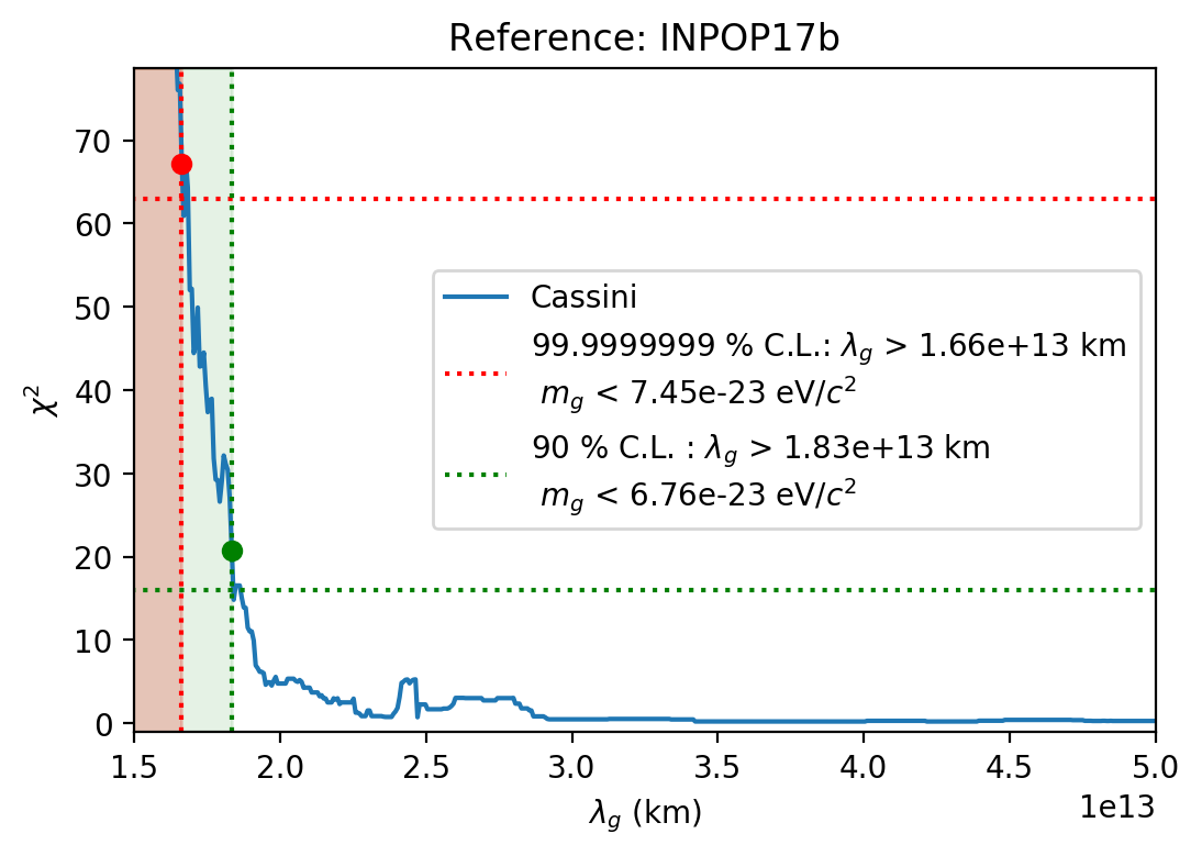
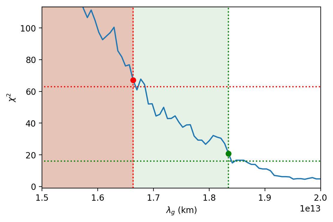
Figure 1: Plot of $\chi^{2}(\lambda_{g})$ and the constraints deduced for $\lambda_{g}$. The probabilities $p=90\%$ and $p=99,9999999\%$ correspond to critical values of $\chi^{2}$ equal to respectively $15.99$ and $62.94$.

———————————————————————

VI Conclusion

In the present manuscript, we deliver the first conservative estimate of the graviton mass from an actual fit of a combination of Solar System data, using a criterion based on a state of the art Solar System ephemerides: INPOP17b. The bound reads $\lambda_{g}>1.83\times 10^{13}$ km (resp. $m_{g}<6.76\times 10^{-23}$ eV/$c^{2}$) with a confidence of 90% and $\lambda_{g}>1.66\times 10^{13}$ km (resp. $m_{g}<7.45\times 10^{-23}$ eV/$c^{2}$) with a confidence of 99.9999999%. As previously explained, in terms of a fifth force, the constraint on $\lambda_{g}$ can be translated into a constraint on $\lambda/\sqrt{\alpha}$, simply by substituting $\lambda_{g}$ by $\lambda/\sqrt{\alpha}$, if $\alpha>0$.

The fact that our 90% C.L. bound is comparable in magnitude to the one obtained by the LIGO-Virgo collaboration in the radiative regime The LIGO Scientific Collaboration and the Virgo Collaboration (2019); Abbott et al. (2017) is a pure coincidence: the two bounds rely on totally different types of observation — gravitational waves versus radioscience in the Solar System — and probe different aspects of the massive graviton phenomenology — radiative versus Keplerian.

References

- Fierz and Pauli (1939) M. Fierz and W. Pauli, “On Relativistic Wave Equations for Particles of Arbitrary Spin in an Electromagnetic Field,” Proceedings of the Royal Society of London Series A 173, 211–232 (1939).
- de Rham et al. (2017) C. de Rham, J. T. Deskins, A. J. Tolley, and S.-Y. Zhou, “Graviton mass bounds,” Reviews of Modern Physics 89, 025004 (2017), arXiv:1606.08462 .
- de Rham (2014) C. de Rham, “Massive Gravity,” Living Reviews in Relativity 17, 7 (2014), arXiv:1401.4173 [hep-th] .
- The LIGO Scientific Collaboration et al. (2018) The LIGO Scientific Collaboration, the Virgo Collaboration, B. P. Abbott, R. Abbott, T. D. Abbott, S. Abraham, F. Acernese, K. Ackley, C. Adams, R. X. Adhikari, and et al., “GWTC-1: A Gravitational-Wave Transient Catalog of Compact Binary Mergers Observed by LIGO and Virgo during the First and Second Observing Runs,” arXiv e-prints (2018), arXiv:1811.12907 [astro-ph.HE] .
- Will (1998) C. M. Will, “Bounding the mass of the graviton using gravitational-wave observations of inspiralling compact binaries,” Phys. Rev. D 57, 2061–2068 (1998), gr-qc/9709011 .
- Del Pozzo et al. (2011) W. Del Pozzo, J. Veitch, and A. Vecchio, “Testing general relativity using Bayesian model selection: Applications to observations of gravitational waves from compact binary systems,” Phys. Rev. D 83, 082002 (2011), arXiv:1101.1391 [gr-qc] .
- The LIGO Scientific Collaboration and the Virgo Collaboration (2019) The LIGO Scientific Collaboration and the Virgo Collaboration, “Tests of General Relativity with the Binary Black Hole Signals from the LIGO-Virgo Catalog GWTC-1,” arXiv e-prints , arXiv:1903.04467 (2019), arXiv:1903.04467 [gr-qc] .
- Will (2018) Clifford M Will, “Solar system versus gravitational-wave bounds on the graviton mass,” Classical and Quantum Gravity 35, 17LT01 (2018).
- Fienga et al. (2008) A. Fienga, H. Manche, J. Laskar, and M. Gastineau, “INPOP06: a new numerical planetary ephemeris,” Astronomy and Astrophysics 477, 315–327 (2008).
- Moyer (2003) T. D. Moyer, Deep Space Communications and Navigation Series, Vol. 2 (John Wiley & Sons, Inc., Hoboken, NJ, USA, 2003).
- Fienga et al. (2011) A. Fienga, J. Laskar, P. Kuchynka, H. Manche, G. Desvignes, M. Gastineau, I. Cognard, and G. Theureau, “The INPOP10a planetary ephemeris and its applications in fundamental physics,” Celestial Mechanics and Dynamical Astronomy 111, 363–385 (2011), arXiv:1108.5546 [astro-ph.EP] .
- Verma et al. (2014) A. K. Verma, A. Fienga, J. Laskar, H. Manche, and M. Gastineau, “Use of MESSENGER radioscience data to improve planetary ephemeris and to test general relativity,” Astronomy and Astrophysics 561, A115 (2014), arXiv:1306.5569 [astro-ph.EP] .
- Fienga et al. (2015) A. Fienga, J. Laskar, P. Exertier, H. Manche, and M. Gastineau, “Numerical estimation of the sensitivity of INPOP planetary ephemerides to general relativity parameters,” Celestial Mechanics and Dynamical Astronomy 123, 325–349 (2015).
- Viswanathan et al. (2018) V. Viswanathan, A. Fienga, O. Minazzoli, L. Bernus, J. Laskar, and M. Gastineau, “The new lunar ephemeris INPOP17a and its application to fundamental physics,” MNRAS 476, 1877–1888 (2018), arXiv:1710.09167 [gr-qc] .
- Viswanathan et al. (2017) V. Viswanathan, A. Fienga, M. Gastineau, and J. Laskar, “INPOP17a planetary ephemerides,” Notes Scientifiques et Techniques de l’Institut de Mecanique Celeste 108 (2017), last Accessed: 2018-11-13.
- Verma and Margot (2016) A. K. Verma and J.-L. Margot, “Mercury’s gravity, tides, and spin from MESSENGER radio science data,” Journal of Geophysical Research (Planets) 121, 1627–1640 (2016), arXiv:1608.01360 [astro-ph.EP] .
- Talmadge et al. (1988) C. Talmadge, J.-P. Berthias, R. W. Hellings, and E. M. Standish, “Model-independent constraints on possible modifications of Newtonian gravity,” Physical Review Letters 61, 1159–1162 (1988).
- Hees et al. (2017) A. Hees, T. Do, A. M. Ghez, G. D. Martinez, S. Naoz, E. E. Becklin, A. Boehle, S. Chappell, D. Chu, A. Dehghanfar, K. Kosmo, J. R. Lu, K. Matthews, M. R. Morris, S. Sakai, R. Schödel, and G. Witzel, “Testing General Relativity with Stellar Orbits around the Supermassive Black Hole in Our Galactic Center,” Physical Review Letters 118, 211101 (2017), arXiv:1705.07902 .
- Pearson (1992) Karl Pearson, “On the criterion that a given system of deviations from the probable in the case of a correlated system of variables is such that it can be reasonably supposed to have arisen from random sampling,” in Breakthroughs in Statistics: Methodology and Distribution, edited by Samuel Kotz and Norman L. Johnson (Springer New York, New York, NY, 1992) pp. 11–28.
- SCOTT (1979) DAVID W. SCOTT, “On optimal and data-based histograms,” Biometrika 66, 605–610 (1979).
- Abbott et al. (2017) B. P. Abbott, R. Abbott, T. D. Abbott, F. Acernese, K. Ackley, C. Adams, T. Adams, P. Addesso, R. X. Adhikari, V. B. Adya, and et al., “GW170104: Observation of a 50-Solar-Mass Binary Black Hole Coalescence at Redshift 0.2,” Physical Review Letters 118, 221101 (2017), arXiv:1706.01812 [gr-qc] .