Optimal probabilistic forecasts for risk management

Abstract

This paper explores the implications of producing forecast distributions that are optimized according to scoring rules that are relevant to financial risk management. We assess the predictive performance of optimal forecasts from potentially misspecified models for i) value-at-risk and expected shortfall predictions; and ii) prediction of the VIX volatility index for use in hedging strategies involving VIX futures. Our empirical results show that calibrating the predictive distribution using a score that rewards the accurate prediction of extreme returns improves the VaR and ES predictions. Tail-focused predictive distributions are also shown to yield better outcomes in hedging strategies using VIX futures.

Keywords: Predictive distributions; scoring rules; value-at-risk; expected shortfall; VIX futures; dynamic risk management

MSC2010 Subject Classification: 60G25, 62M20, 91G70

JEL Classifications: C18, C53, C58.

1 Introduction

Probabilistic forecasts – produced via full predictive probability distributions – provide complete information about the future values of a random variable. Conventional approaches to probabilistic prediction have assumed: either that the predictive model (or likelihood function) correctly specifies the true data generating process (DGP), or that some specified set of predictive models spans the truth; neither of which is likely to be the case in practice.

Optimal probabilistic forecasts, on the other hand, are based on predictive distributions that are optimal in some user-specified proper scoring rule (Gneiting et al.,, 2005; Gneiting and Raftery,, 2007; Patton,, 2019; Martin et al.,, 2022; Zischke et al, 2022). That is, instead of defaulting to the conventional use of a (misspecified) likelihood function, such forecasts exploit a criterion function built from a scoring rule that rewards the type of predictive accuracy that matters for the problem at hand. Optimization may occur with respect to: the parameters of a given model, the weights of a combination of predictive models, or both. In the case of weighted combinations, the approach forms part of a broader push – based on both Bayesian and frequentist principles – to construct forecast combinations that are explicitly designed to perform well according to a particular forecasting metric (see Loaiza-Maya et al.,, 2021 for a recent contribution, and relevant coverage of the literature; and Aastveit et al.,, 2018 and Wang et al.,, 2022 for more extensive reviews).

In short, optimal probabilistic forecasts aim to produce predictions that are accurate in the way that matters, irrespective of the specification of the predictive model (or set of predictive models). In the context of financial risk management, for example, the tails of the predictive distribution of a financial return are of particular interest, with the lower tail capturing the risk of loss in a long (buying) position, while the upper tail captures the risk of loss in a short-selling position. To date, the literature on risk prediction has focused on the development of alternative models that better capture the tail features of returns via: alternative specifications for volatility (e.g. Ding et al.,, 1993, and Hansen et al.,, 2012), alternative conditional distributions for the return (e.g. Chen et al.,, 2008, and BenSaïda et al.,, 2018), the addition of more latent factors (Maheu and McCurdy,, 2004, and Maneesoonthorn et al.,, 2017), or specifications that model only specific quantiles (Engle and Manganelli,, 2004) or specific tail regions (Brooks et al.,, 2005). Scoring rules that are relevant to the tails may then be used to evaluate the forecasts, but do not play a role in the construction of the forecasts themselves (see Giacomini and Komunjer,, 2005, Jensen and Maheu,, 2013, and Chiang et al.,, 2021, amongst many others, including those already referenced above).

In this paper, we take a difference stance. We adopt a predictive model that is known to miss certain critical features of a financial return – namely a generalized autoregressive conditional heteroscedastic (GARCH) model with Gaussian innovations (Bollerslev,, 1987) – but which is simple and quick to estimate. We then calibrate the model using proper scoring rules that are relevant to the tail region in question, and construct an optimal predictive accordingly. We show how calibrating a Gaussian GARCH(1,1) model to tail-focused scoring rules can yield accurate predictions of extreme returns, and illustrate how the results vary with the degree of model misspecification. We also assess the ability of the optimal predictives to produce accurate predictions of value-at-risk (VaR) and expected shortfall (ES) predictions, and compare that accuracy with likelihood-based (or, equivalently, logarithmic score (LS)-based) probabilistic forecasts. We employ two specific tail-focused rules for the construction of optimal forecasts: the censored likelihood score (CLS) of Diks et al., (2011) and the quantile score (QS) (Giacomini and Komunjer,, 2005, and Gneiting and Raftery,, 2007). The CLS is a proper scoring rule that allows a forecaster to focus on accuracy in any particular region of interest, including the tail of the predictive distribution. As a proper scoring rule for quantiles, the QS is also particularly relevant here for the production of VaR predictions, having also been used previously as the criterion function in the estimation of quantile regressions (Koenker and Bassett,, 1978 and Engle and Manganelli,, 2004). The VaR and ES predictions are assessed using the conditional coverage test of Christoffersen, (1998) and the recently proposed ES predictive dominance test of Ziegel et al., (2020), respectively.

We then extend our application of optimal forecasts to the problem of predicting the option-implied volatility index (VIX), and producing effective hedging strategies based on VIX derivatives (Moran and Liu,, 2020; Konstantinidi et al.,, 2008; Taylor,, 2019). Once again, we depart from the idea of seeking an ideal predictive model for the index (Konstantinidi et al.,, 2008; Fernandes et al.,, 2014; Taylor,, 2019), instead constructing optimal forecasts using the simple heterogenous autoregressive (HAR) model of Corsi, (2009) with Gaussian GARCH(1,1) errors. In this case we use the CLS score to calibrate the model – and produce the optimal predictive – but with the region of ‘focus’ designed to match certain features of the trading strategy in question.

The paper proceeds as follows. Section 2 explains how scoring rules are used to construct optimal distributional forecasts, as well as outlining the specific tail-focused rules that are relevant to financial risk management. Section 3 investigates the benefits yielded by optimal forecasting in a simulation setting, paying particular attention to how well the optimal forecasts perform in predicting tail risks via the assessment of VaR and ES predictions for a financial return. Model misspecification is explicitly factored into the simulation design with a view to replicating a realistic empirical scenario. An extensive empirical analysis of 12 S&P market and industry indices is then conducted in Section 4, with the results confirming our simulation findings in Section 3: i.e. that the optimal predictives achieve substantially better tail risk predictions than the likelihood-based alternatives. In Section 5, we explore the use of optimal forecasts of the VIX index in the construction of effective hedging strategies using recent data on the VIX index and VIX futures. The ability of the tailored score-based predictives to achieve better investment outcomes highlights the practical importance of optimal forecasting in risk management. We conclude in Section 6.

2 Scoring Rules in Risk Prediction

2.1 Scoring Rules and the Optimal Forecast Distribution

Scoring rules (Gneiting and Raftery,, 2007) are measures of performance for probabilistic forecasts. As such, they are often used to evaluate and rank competing probabilistic forecasts, based on materialized events or values, by assigning a numerical score. That is, if a forecaster produces a predictive distribution $\mathit{P}$ and the event $y$ materializes, then the reward for this prediction given by a scoring rule is denoted by $S(P,y)$. For a positively-oriented score, a higher value will be assigned to the better of two competing predictions, on the condition of the scoring rule being proper. The propriety of the scoring rule is crucial here, as an improper scoring rule may assign a higher average score to an incorrect prediction, i.e. one that does not tally with the true DGP.

More formally, suppose $P$ is the predictive distribution and $Q_{0}$ is the true DGP. $\mathbb{S}(P,Q_{0})$ denotes the expected value of $S(P,\cdot)$ under $Q_{0}$. That is,

$$\mathbb{S}(P,Q_{0})=\int_{y\in\Omega}S(P,y)dQ_{0}(y)$$ (1)

where $\Omega$ is the sample space. A scoring rule is said to be proper if $\mathbb{S}(Q_{0},Q_{0})\geq\mathbb{S}(P,Q_{0})$ for all $P$ and $Q_{0}$, and is strictly proper if $\mathbb{S}(Q_{0},Q_{0})=\mathbb{S}(P,Q_{0})$ only when $P=Q_{0}$ (Gneiting and Raftery,, 2007). This ensures that a proper scoring rule is maximized when the prediction reveals the truth, on the condition that the predictive distribution class $\mathcal{P}$ contains $Q_{0}$.

In practice of course, the expected score $\mathbb{S}(\cdot,Q_{0})$ cannot be obtained, but we can use a sample average of observed scores as a reasonable estimator. Asymptotically, the true predictive distribution can be recovered by optimizing a sample criterion based on any proper scoring rule, if the true predictive is contained in the predictive class over which the maximization occurs. Even when $Q_{0}$ is not contained in the predictive distribution class $\mathcal{P}$ proposed by the forecaster, it does not change the fact that a proper scoring rule will reward a particular form of forecast accuracy and, hence, optimization will select the best forecast within the predictive class, according to this scoring rule.

Thus, a scoring rule can be used to define a criterion function that can be optimized to obtain parameter estimates, from which a probabilistic prediction that is optimal in that score can be produced. Assume that the scoring rule is positively-oriented and the unknown parameters of the assumed predictive model are denoted as $\boldsymbol{\theta}\in\Theta$, and let $P_{\boldsymbol{\theta}}^{t-1}$ := $P(\cdot|\mathcal{F}_{t-1},\boldsymbol{\theta})$ be the one-step-ahead predictive distribution function based on the assumed model, where $\mathcal{F}_{t-1}$ represents all the information available at time $t-1$, and $p(\cdot|\mathcal{F}_{t-1},\boldsymbol{\theta})$ be the corresponding predictive density function at time $t$. For $\tau$ such that $T\geq\tau\geq 1$, let $\{y_{t}\}_{t=1}^{T-\tau}$ denote a series of size $T-\tau$ used for the optimization, with $\tau$ denoting the size of a hold-out sample. Defining:

$$\bar{S}(\boldsymbol{\theta})=\frac{1}{T-(\tau+1)}\sum_{t=2}^{T-\tau}S(P_{\boldsymbol{\theta}}^{t-1},y_{t}),$$ (2)

then an estimator $\boldsymbol{\hat{\theta}}$ obtained by maximizing $\bar{S}(\boldsymbol{\theta})$:

$$\boldsymbol{\hat{\theta}}=\text{arg}\max_{\boldsymbol{\theta}\in\Theta}\bar{S}(\boldsymbol{\theta})$$ (3)

is said to be “optimal” based on this scoring rule, and $P_{\boldsymbol{\hat{\theta}}}^{t-1}$ is referred to as the optimal predictive. Under certain conditions, including that the scoring rule is proper and that the predictive model is correctly specified, $\boldsymbol{\hat{\theta}}\rightarrow\boldsymbol{\theta}_{0}\ \text{as}\ \mathit{T}\rightarrow\infty$ (for a fixed $\tau$), where $\boldsymbol{\theta}_{0}$ represent the true (vector) parameter. If the predictive model is misspecified, then $\boldsymbol{\hat{\theta}}$ converges to $\boldsymbol{\theta_{\ast}}$, where the latter denotes the maximum of the limiting criterion function to which $\bar{S}(\boldsymbol{\theta})$ converges as $T$ diverges. (Gneiting and Raftery,, 2007; Martin et al.,, 2022; Zischke et al, 2022.)

2.2 Scoring Rules for Financial Risk Predictions

In risk management applications, the region of interest is typically in the tails of the distribution, with the lower tail being relevant to the risk of loss in long positions and the upper tail relevant to the risk of loss in short positions. The censored logarithmic score (CLS) of Diks et al., (2011) allows users to reward accurate forecasts in a particular region (or regions) of interest, such as an upper or lower tail. It is defined as

$$S_{CLS}(P_{\boldsymbol{\theta}}^{t-1},y_{t})=I(y_{t}\in A)\log\left(p(y_{t}|\mathcal{F}_{t-1},\boldsymbol{\theta})\right)+I(y_{t}\in A^{c})\log\left(\int_{y\in A^{c}}p(y|\mathcal{F}_{t-1},\boldsymbol{\theta})dy\right),$$ (4)

where $A$ is the region of interest and $A^{c}$ is its complement. The CLS has been applied in the evaluation of predictive distributions geared to risk management (Jensen and Maheu,, 2013, and Chiang et al.,, 2021), as well as in inferential procedures geared to certain data regions (Gatarek et al.,, 2014, and Borowska et al.,, 2020). Opschoor et al., (2017) have also applied the CLS in the estimation of forecast combinations and found that density forecasts based on optimizing the CLS outperform alternatives forecasts that are not constructed to reward tail accuracy (see also Loaiza-Maya et al.,, 2021).

A feature of the predictive distribution that is critically important in financial risk management is the VaR: computed (in the case of one-step-ahead prediction) as the $p\times 100\%$ quantile of the one-step-ahead predictive distribution ${P_{\boldsymbol{\theta}}^{t-1}}$, and denoted by $VaR_{p}(P_{\boldsymbol{\theta}}^{t-1})$. The quantile score (QS) is a proper score for quantiles and is thus particularly suitable for rewarding accurate prediction of the VaR (see, for example, Giacomini and Komunjer,, 2005, Bao et al.,, 2006 and Laporta et al.,, 2018). The QS is defined, in turn, as

$$S_{QS}(P_{\boldsymbol{\theta}}^{t-1},y_{t})=\left[I(y_{t}\leq VaR_{p}(P_{\boldsymbol{\theta}}^{t-1}))-p\right]\left(y_{t}-VaR_{p}(P_{\boldsymbol{\theta}}^{t-1})\right).$$ (5)

In this paper, we investigate whether calibrating the model to the tail-focused proper scoring rules, such as (the appropriately specified) CLS and QS, yields accurate probabilistic forecasts for financial risk management. As a comparator we adopt the LS, defined as

$$S_{LS}(P_{\boldsymbol{\theta}}^{t-1},y_{t})=\log\left(p(y_{t}|\mathcal{F}_{t-1},\boldsymbol{\theta})\right),$$ (6)

which, as a ‘local’ scoring rule, will assign a high value if the realized value of $y_{t}$ is in the high density region of $p\left(y_{t}|\mathcal{F}_{t-1},\boldsymbol{\theta}\right)$ and a low value otherwise. A sample criterion defined using the log score is equivalent to the log-likelihood function. Thus, optimization with respect to the LS yields the maximum likelihood estimator of $\boldsymbol{\theta}$ as

$$\boldsymbol{\hat{\theta}}_{MLE}=\text{arg}\max_{\boldsymbol{\theta}\in\Theta}\left\{\frac{1}{T-(\tau+1)}\sum_{t=2}^{T-\tau}\log\left(p(y_{t}|\mathcal{F}_{t-1},\boldsymbol{\theta})\right)\right\},$$ (7)

which, under the assumption of correct specification (and regularity), is the asymptotically efficient estimator of $\boldsymbol{\theta}_{0}$; hence the interest in documenting the performance of what may be viewed as the conventional approach to the construction of a predictive density.

Finally, we note that the expected shortfall (ES) is a point forecast that is often reported alongside the VaR to evaluate the tail risk in financial investments, and is considered to be a robust risk measurement, given its coherence properties (see Acerbi and Tasche,, 2002, Tasche,, 2002, and Yamai and Yoshiba,, 2005). By definition, the $p^{th}$ ES constructed from the one-step-ahead predictive distribution $P_{\boldsymbol{\theta}}^{t-1}$ is defined as

$$ES_{p}(P_{\boldsymbol{\theta}}^{t-1})=\frac{1}{p}\int_{0}^{p}VaR_{\alpha}(P_{\boldsymbol{\theta}}^{t-1})d\alpha,$$ (8)

where $VaR_{\alpha}(P_{\boldsymbol{\theta}}^{t-1})$ denotes the $\alpha\times 100\%$ quantile of the predictive distribution. The ES is not elicitable as a point forecast, implying that there is no scoring function that allows for a consistent ranking of model performance based on ES alone (Gneiting,, 2011). However, Fissler et al., (2015) propose a class of scoring functions that can jointly elicit the forecast accuracy of VaR and ES, and can thus be used to measure ES predictive accuracy (in conjunction with that of VaR). The joint scoring function for $VaR_{p}(P_{\boldsymbol{\theta}}^{t-1})$ and $ES_{p}(P_{\boldsymbol{\theta}}^{t-1})$, in positive orientation, is defined as

$$S_{\eta}(P^{t-1}_{\boldsymbol{\hat{\theta}}},y_{t})=-I(\eta\leq ES_{p}(P^{t-1}_{\boldsymbol{\hat{\theta}}})) \left(\frac{1}{p}I(y_{t}\leq VaR_{p}(P^{t-1}_{\boldsymbol{\hat{\theta}}}))(VaR_{p}(P^{t-1}_{\boldsymbol{\hat{\theta}}})-y_{t})\right.$$ (9)

$$-\left.(VaR_{p}(P^{t-1}_{\boldsymbol{\hat{\theta}}})-\eta)\right)-I(\eta\leq y_{t})(y_{t}-\eta).$$

Here, the scoring function is indexed by the real number $\eta$ that spans the range of the random variable of interest, with the dominance of one predictive model over another (in terms of ES accuracy) gauged by values of their respective scores over a relevant range of $\eta$ (see Ehm et al.,, 2016, and Ziegel et al.,, 2020). Whilst we do not use this scoring function to determine the criterion used to produce an estimate of $\boldsymbol{\theta}$ and, ultimately, the corresponding optimal predictive, we do adopt this scoring function to compare the accuracy of the ES (and VaR) predictions produced by the relevant tail-focused predictives, with the accuracy of those produced by the LS- (or MLE-based) predictive.

3 Performance of Score-Based Risk Predictions: Simulation Evidence

Forecasts explicitly designed to reward certain types of accuracy – whether it be via the optimization advocated in this paper, or via a suitable (“focused”) Bayesian posterior up-date – can certainly outperform predictions produced by conventional methods; see Opschoor et al., (2017), Loaiza-Maya et al., (2021), and Martin et al., (2022). In simulation settings it has been shown that the degree of model misspecification has a notable effect on the performance of optimal forecasts. In short, the greater the degree of misspecification, the greater the gain from optimal (or focused) forecasts, at least conditional on the assumed predictive model being broadly “compatible” with the true DGP. This result augurs well for the usefulness of such targeted predictions in empirical settings, in which misspecification is unavoidable, and this provides strong motivation for the analysis undertaken herein – in which optimal predictions are sought in empirical risk management settings. In this section, we evaluate the performance of the optimal tail-focused forecasts, relative to the conventional MLE-based forecast, in terms of their ability to predict tail risks in a simulation setting. Whilst the MLE-based predictive is formally “optimal” with respect to the LS, we reserve the term “optimal” hereafter for the predictives based on the tail-focused scores.

3.1 Simulation Design

We generate $T$ observations of a random variable $y_{t}$ from three alternative true DGPs, each of which captures the main stylized features of a financial return and its volatility. A GARCH model of order (1,1) with Gaussian errors is used to define the predictive class $\mathcal{P}$ in all experiments. Scenario (i) represents the case of correct specification, with the true DGP matching the predictive model is this case. Scenario (ii) uses a GARCH(1,1) model with Student-t errors as the true DGP, thereby representing the case of mispecification of the fourth moment. Finally, in Scenario (iii) the skewed stochastic volatility model introduced by Smith and Maneesoonthorn, (2018), and also used in Loaiza-Maya et al., (2021), is used as the true DGP. This model assumes a skew-normal marginal distribution, which allows us to measure the performance of the optimal forecasts under misspecification of the third moment of the data, in addition to the use of an incorrect conditionally deterministic volatility specification. Under each of Scenarios (ii) and (iii), we vary the degree of misspecification by changing the degrees of freedom in the Student-t distribution and the shape parameter in the skew-normal distribution, respectively. Details of each of these scenarios are given in Table 1.

Table 1: The three simulation scenarios used in the numerical analysis. The assumed predictive model is GARCH(1,1) in all cases, and the true DGP is varied across the scenarios. Scenario (i) represents correct model specification. Scenario (ii) represents the first form of misspecification, where $t_{\nu}$ indicates a Student-t distribution, with the degrees of freedom parameter, $\nu$, assuming values of 3 and 12. Scenario (iii) represents the second form of misspecification, with the shape parameter in the skew-normal marginal return distribution assuming the values of 0 (representing a symmetric marginal distribution), and -3 and -5 (which produce, in turn, increasing negative skewness in the marginal distribution.

	Scenario (i)		Scenario (ii)		Scenario (iii)
True DGP	$y_{t}=\sigma_{t}\epsilon_{t}$		$y_{t}=\sigma_{t}\epsilon_{t}$		$y_{t}=D^{-1}(F_{z}(z_{t}))$
	$\sigma_{t}^{2}=1+0.2y_{t-1}^{2}+0.7\sigma^{2}_{t-1}$		$\sigma_{t}^{2}=1+0.2y_{t-1}^{2}+0.7\sigma_{t-1}^{2}$		$z_{t}=\exp(h_{t}/2)\epsilon_{t}$, $\epsilon_{t}\sim i.i.d.N(0,1)$
	$\epsilon_{t}\sim i.i.d.N(0,1)$		$\epsilon_{t}\sim i.i.d.(\frac{\nu-2}{\nu})^{0.5}*t_{\nu}$		$h_{t}=-0.4581+0.9(h_{t-1}+0.4581)+0.4172\eta_{t}$, $\eta_{t}\sim i.i.d.N(0,1)$
			$\nu\in\{3,12\}$		$D(.)$ is the CDF of a skew-normal distribution
					with shape parameter $\in\{0,-3,-5\}$
Assumed model	$y_{t}=\mu+\sigma_{t}\epsilon_{t}$		$y_{t}=\mu+\sigma_{t}\epsilon_{t}$		$y_{t}=\mu+\sigma_{t}\epsilon_{t}$
	$\sigma_{t}^{2}=\alpha_{0}+\alpha_{1}(y_{t-1}-\mu)^{2}+\beta_{1}\sigma_{t-1}^{2}$		$\sigma_{t}^{2}=\alpha_{0}+\alpha_{1}(y_{t-1}-\mu)^{2}+\beta_{1}\sigma_{t-1}^{2}$		$\sigma_{t}^{2}=\alpha_{0}+\alpha_{1}(y_{t-1}-\mu)^{2}+\beta_{1}\sigma_{t-1}^{2}$
	$\epsilon_{t}\sim i.i.d.N(0,1)$		$\epsilon_{t}\sim i.i.d.N(0,1)$		$\epsilon_{t}\sim i.i.d.N(0,1)$

We estimate optimal forecasts under all three scenarios using the two proper scoring rules introduced in Section 2.2: the CLS and the QS. For the CLS, we focus on the 10% lower tail, corresponding to the risk associated with a long financial position, and we label this as CLS10 hereafter. In order to mimic the situation that prevails in practice, in which the true predictive is unknown, the region $A$, required for evaluation of the CLS, is based on a marginal empirical quantile rather than a conditional quantile. The QS is used as the scoring rule that targets the predictive accuracy of a $p\times 100\%$ conditional quantile. We consider quantiles that are relevant to the computation of VaR and ES quantities in practice, by specifying $p\times 100\%=\{2.5\%,5\%,10\%\}$. We label these three versions of QS as QS2.5, QS5 and QS10 respectively. Because the LS-based predictive gives us insight into the performance of the conventional MLE method, it is used as a benchmark for assessing the improvement of the optimal forecasts.

Let $P_{\boldsymbol{\hat{\theta}_{i}}}^{t-1}$ denote the one-step-ahead predictive distribution function based on the Gaussian GARCH(1,1) model, optimized according to scoring rule $S_{i}$. For each of the true DGPs specified in Table 1, we draw $T=6000$ observations of $y_{t}$ from $Q_{0}$. Given $\tau=5000$, we then utilize expanding estimation windows, beginning with a sample of size 999, to obtain the optimal one-step-ahead predictive $P_{\boldsymbol{\hat{\theta}_{i}}}^{t-1}$, for $t=T-\tau+1,...,T$. For each $t$, $\boldsymbol{\hat{\theta}}_{i}=\{\hat{\mu},\hat{\alpha}_{0},\hat{\alpha}_{1}\}_{i}$ is obtained as in (3) and (2) for $S_{i}\in\{LS,CSL10,QS2.5,QS5,QS10\}$. We then document the relative performance of the MLE-based predictive and the optimal predictives in two ways. First, we assess the performance of all in producing accurate VaR predictions by conducting the conditional coverage test of Christoffersen, (1998). Forecasts that produce VaR exceedences that are insignificantly different from the nominal $p$ level, and that are uncorrelated over time, are deemed to be desirable. Second, we evaluate the accuracy of the ES forecasts using the scoring rule defined in (9), along with the Murphy diagram of Ehm et al., (2016) and Ziegel et al., (2020), where, as noted earlier, this diagram is designed to assess the ES predictive dominance of one predictive over another.

3.2 Value-at-Risk Assessment

In this section, we assess the accuracy of the 2.5%, 5% and 10% VaR predictions constructed from the predictive densities $P_{\boldsymbol{\hat{\theta}_{i}}}^{t-1}$, for $S_{i}\in\{LS,CLS10,QS2.5,QS5,QS10\}$. The empirical tail coverage and conditional coverage test results are documented in Table 2. The bolded values indicate instances where the null hypothesis of the conditional coverage test is not rejected at the 5% significance level. The bolded italicized value in a given column indicates the (insignificant) result with the empirical tail coverage that is the closest to the nominal coverage.

Panel A of Table 2 reports the results for the correctly specified case. As anticipated, given that all scoring rules are proper, and the (expanding) estimation samples are large, optimization of (2) – for each choice of score – produces a value for $\boldsymbol{\hat{\theta}}$ that is close to the true value of $\boldsymbol{\theta}_{0}$; hence all predictives are very similar and have comparable out-of-sample performance, however measured – and this is what we see (overall) in the Panel A results.

In contrast, if one considers what is arguably the most misspecified case – Scenario (iii) with shape parameter of -5 – with results reported in Panel F, we see evidence of what Martin et al., (2022) refer to as “strict coherence”. That is, the scoring rule designed to yield optimal predictions according to a particular measure produces the best performance out of sample in terms of that measure. Specifically, the QS($p\times 100$)-based predictive produces the most accurate prediction of the VaR at that nominal level, for each value of $p.$ Moreover, the CLS10-based predictive – which focuses on lower tail accuracy per se – performs almost as well as each QS($p\times 100$)-based predictive, yielding an empirical coverage that is insignificantly different from the nominal value for all three VaRs considered. In the case of Scenario (ii), Panel C, in which the misspecification manifests itself via a very fat-tailed Student-t innovation that is not matched by the (conditionally) Gaussian predictive model, strict coherence is also in evidence for the 5% and 10% VaRs.

For the remaining misspecified cases, there is certainly some evidence that the tail-focused scores reap benefits out-of-sample in terms of VaR prediction. Most notably, the QS-based optimal forecasts always accurately predict the relevant VaR (i.e. the corresponding values recorded in the table are always bolded), independent of the degree of misspecification; that is, even if the QS-based predictive is not the most accurate in every single case, it never behaves poorly, auguring well for the blanket use of a QS-based predictive in empirical settings in which accurate VaR coverage is the goal.

Table 2: Predictive performance for VaR under Scenarios (i)-(iii) in Table 1. The numbers reported are the proportion of exceedances. The bold font is used to indicate exceedances that are not significantly different from the nominal level and are uncorrelated over time, resulting in a failure to reject the null hypothesis of the conditional coverage test, at the 5% level of significance. The (bolded) italicized value in a given column is the exceedance that fails to reject the null hypothesis of the conditional coverage test and is closest to the nominal $p$ level.

. Out-of-sample exceedances Optimizers VaR at 2.5% VaR at 5% VaR at 10% VaR at 2.5% VaR at 5% VaR at 10% Panel A: Scenario (i) Panel D: Scenario (iii) with Shape=0 MLE 2.94% 5.24% 10.18% 2.30% 5.12% 10.82% CLS10 3.26% 5.52% 9.98% 2.42% 5.12% 10.46% QS2.5 2.98% 4.86% 9.36% 2.56% 5.38% 10.76% QS5 3.38% 5.70% 10.00% 2.46% 5.14% 10.72% QS10 3.50% 5.90% 10.60% 2.26% 4.66% 10.46% Panel B: Scenario (ii) with $\nu$ = 12 Panel E: Scenario (iii) with Shape=-3 MLE 2.98% 5.38% 9.72% 4.10% 7.08% 11.76% CLS10 2.78% 5.28% 10.00% 2.50% 5.10% 9.54% QS2.5 2.82% 4.88% 9.06% 2.54% 4.62% 8.60% QS5 3.10% 5.32% 9.40% 2.88% 5.24% 9.16% QS10 3.80% 6.06% 10.40% 3.52% 6.06% 10.38% Panel C: Scenario (ii) with $\nu$ = 3 Panel F: Scenario (iii) with Shape=-5 MLE 2.70% 4.00% 7.06% 4.54% 7.66% 12.06% CLS10 2.14% 4.24% 10.96% 2.66% 5.24% 9.48% QS2.5 2.92% 4.32% 7.24% 2.58% 4.70% 8.22% QS5 4.10% 5.28% 7.96% 2.80% 5.20% 8.88% QS10 6.20% 7.78% 10.14% 3.72% 6.26% 10.38%

3.3 Expected Shortfall Assessment

Based on (9), Ziegel et al., (2020) propose the concept of “forecast dominance” for comparative assessment of joint pairs of VaR and ES. The predictive $P_{\boldsymbol{\hat{\theta}_{i}}}^{t-1}$ is deemed to weakly dominate the predictive $P_{\boldsymbol{\hat{\theta}_{j}}}^{t-1}$, when $E[S_{\eta}(P_{\boldsymbol{\hat{\theta}_{i}}}^{t-1},y_{t})]\geq E[S_{\eta}(P_{\boldsymbol{\hat{\theta}_{j}}}^{t-1},y_{t})]$ for any value of $\eta$. We follow Ziegel et al., (2020) in assessing the dominance of competing predictives using the Murphy diagram, where the horizontal axis is $\eta$ and the vertical axis is the average score difference constructed as

$$\Delta_{\eta}\left(P_{\boldsymbol{\hat{\theta}_{i}}}^{t-1},P_{\boldsymbol{\hat{\theta}_{MLE}}}^{t-1}\right)=\widehat{E}\left[S_{\eta}(P_{\boldsymbol{\hat{\theta}_{i}}}^{t-1},y_{t})\right]-\widehat{E}\left[S_{\eta}(P_{\boldsymbol{\hat{\theta}_{MLE}}}^{t-1},y_{t})\right],$$ (10)

where the expectations are estimated as the sample mean of the relevant out-of-sample scores, in the usual way. In order to keep the analysis manageable, we compute (10) for $p=0.1$ only, and using the optimal predictive, $P_{\boldsymbol{\hat{\theta}_{i}}}^{t-1}$, computed using CLS10 and QS10 respectively. In each case, the comparator (as made clear from the notation used in (10)) is the MLE-based predictive. Once again, results are presented for all scenarios in Table 1.

The Murphy diagrams for Scenarios (i) and (ii) are presented in Figure 1 and the diagrams for Scenario (iii) are depicted in Figure 2. The left hand column in each case depicts the difference between the optimal QS10 predictive and the MLE predictive; while the right hand column depicts the difference between the CLS10 predictive and the MLE predictive. In each diagram, the average ES score difference is presented as the solid black line, the bootstrapped 95% confidence interval is shaded in grey, and the benchmark of zero is the horizontal dotted red line.

In Figure 1, the QS10 optimal predictive dominates the MLE predictive over a reasonable range of $\eta$ for the most misspecified case in Scenario (ii), with $\nu=3$ (Panel E). The CLS10 predictive, on the other hand, generates average scores that are larger in magnitude than those of the MLE predictive, but the difference is not statistically significant (Panel F). In the correctly specified and mildly misspecified cases (Panels A - D), we do not observe a significant difference between either tail-focused predictive and the MLE predictive.

Under Scenario (iii), we observe clearer benefits overall from using the QS10 and CLS10 optimal predictives rather than the MLE predictive. As is to be expected, when the true predictive is symmetric (Panels A and B), we do not observe significant differences between the optimal and MLE average scores. However, as the true predictive becomes more asymmetric (with non-zero shape parameters), we observe a clear dominance of the QS10 and CLS10 optimal predictives over the MLE predictive, as seen in Panels C - F in Figure 2. In addition, the average score differences for the QS10 predictives are larger in magnitude than the corresponding average score difference for the CLS10 predictives in these cases. This suggests that calibrating the predictive distribution using the QS score yields greater benefits in terms of accurate (joint) ES and VaR prediction than using the CLS10 score. This conclusion is further supported by the observation that the (greater) dominance (over the MLE predictive) of the QS10 predictive relative to the CLS10 predictive coincides with the fact that the former performs better overall than the latter in terms of the VaR assessment in Section 3.2 (see Panel F, in particular, in Table 2).

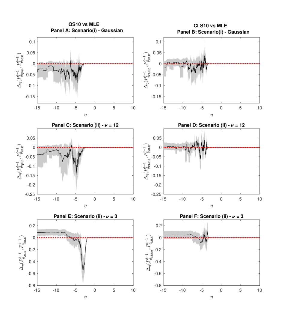
Figure 1: 10% ES predictive performance for the DGPs in Scenario (i) and (ii) in Table 1. Each panel depicts the Murphy diagram, plotting $\Delta_{\eta}\left(P_{\boldsymbol{\hat{\theta}_{i}}}^{t-1},P_{\boldsymbol{\hat{\theta}_{MLE}}}^{t-1}\right)$ against $\eta$, with the shaded area being the 95% bootstrapped confidence interval. The left hand side column assesses the QS10 predictive relative to the MLE predictive, and the right hand side panel assesses the CLS10 predictive relative to the MLE

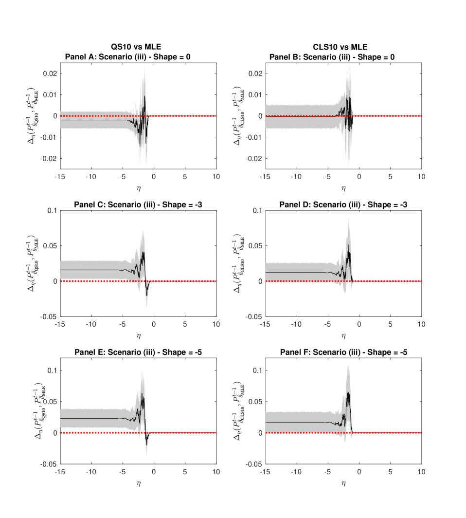
Figure 2: 10% ES predictive performance for the DGPs in Scenario (iii) in Table 1. Each panel depicts the Murphy diagram, plotting $\Delta_{\eta}\left(P_{\boldsymbol{\hat{\theta}_{i}}}^{t-1},P_{\boldsymbol{\hat{\theta}_{MLE}}}^{t-1}\right)$ against $\eta$, with the shaded area being the 95% bootstrapped confidence interval. The left hand side column assesses the QS10 predictive relative to the MLE predictive, and the right hand side panel assesses the CLS10 predictive relative to the MLE

4 Empirical Analysis of Financial Returns

In Section 3, using artificial data that mimic the features of financial returns, we have illustrated the benefit of calibrating the predictive distribution using the score that is appropriate for the application of the prediction. In particular, we have observed that the higher the degree of misspecification, the greater the benefit reaped by optimal forecasting in this setting.

In this section, we produce optimal predictive distributions for returns on a range of empirical financial indices: Standard and Poor’s S&P500, S&P Small Cap, S&P Mid Cap and its nine industry indices, using the Gaussian GARCH(1,1) model as the predictive model. Specifically, we document the improvement in predictive performance that can be yielded by calibrating the GARCH(1,1) model to scoring rules that focus predictive performance on the sort of accuracy that matters in financial settings, despite the likely misspecification of the predictive model itself. We adopt the following scores in all of the empirical analysis, $S_{i}\in\{LS,CSL10,CLS20,CLS80,CSL90,QS2.5,QS5,\linebreak QS10\}$. In Section 4.2 we assess the coherence of the predictive returns distributions to the scoring rule used for calibration – by matching the score used to compute the out-of-sample average performance to the score used for callibration. In Section 4.2 and 4.4 respectively we document the improved accuracy of VaR and ES predictions that can be yielded by the use of tail-focused scores.

4.1 Data Description

We consider the time period between 14 August 1996 to 30 July 2020 in our empirical analysis. The data on the S&P500 index are taken from Yahoo Finance, and data on all indices obtained from the Global Financial Data (GFD) database. We construct 6000 continuously-compounded daily return observations for each index, keeping the first 1000 observations for the initial training sample and the latter 5000 observations for out-of-sample predictive evaluations. Expanding estimation windows are used, as in the simulation exercise. The out-of-sample period between 1 August 2000 and 30 July 2020 includes two very volatile periods: the global financial crisis (GFC) and the recent COVID-19 pandemic.

Table 3 provides the details of the 12 indices we investigate, and the descriptive statistics for all returns series. All twelve return series are non-Gaussian, as evidenced by the rejections of the Jarque-Bera test. As to be expected with daily financial returns, fat tails are a prominent feature. We also observe negative skewness in all but the S&P45 index. The Ljung-Box test for serial correlation in the squared returns is also indicative of time-varying volatility for all series.

Table 3: Descriptions and summary statistics of the 12 S&P indices under investigation. Summary statistics include the mean, the standard deviation (Std), and skewness and kurtosis statistics. The JB.Test column reports the p-value of the Jarque-Bera test for normality and the LB.test column reports the p-value of the test of serial correlation of the squared returns with 20 lags.

Index	Description	Mean	Std	Skewness	Kurtosis	JB.Test	LB.Test
S&P500	S& 500 Market Index	0.026	1.243	-0.394	13.467	0.000	0.000
S&P Small Cap	S&P Small Capitalization Index	0.031	1.244	-0.553	10.938	0.000	0.000
S&P Mid Cap	S&P Mid Capitalization Index	0.034	1.444	-0.635	13.147	0.000	0.000
S&P15	S&P Materials Index	0.018	1.359	-0.323	10.270	0.000	0.000
S&P20	S&P Industrial Index	0.023	1.527	-0.419	10.857	0.000	0.000
S&P25	S&P Consumer Discretionary Index	0.035	1.373	-0.274	11.194	0.000	0.000
S&P30	S&P Consumer Staples Index	0.025	1.378	-0.175	13.683	0.000	0.000
S&P35	S&P Health Care Index	0.034	0.997	-0.197	10.152	0.000	0.000
S&P40	S&P Financial Index	0.015	1.216	-0.178	18.230	0.000	0.000
S&P45	S&P Information Technology Index	0.042	1.915	0.063	9.236	0.000	0.000
S&P50	S&P Telecommunication Services Index	0.007	1.772	-0.044	9.941	0.000	0.000
S&P55	S&P Utilities Index	0.016	1.232	-0.096	16.298	0.000	0.000

4.2 Performance of Optimal Prediction of Returns

Table 4 summarizes the out-of-sample predictive performance of the GARCH(1,1) model for all 12 indices, and as measured by all eight scoring rules. For each series, and in a particular column, we report two numbers: i) the the average out-of-sample score for the MLE-based predictive, and ii) the average out-of-sample score for the predictive that is calibrated to the score used to measure performance, with this predictive referred to as the “optimal” predictive. In the first column, for each series, both of these numbers are automatically equivalent, given that the score in question is the LS, and the MLE-based predictive is optimal according to the LS. In all other columns, the numbers typically differ. The bolded value for a given series, and in a given column, indicates the predictive (MLE-based or optimal) that generates the higher average score over the out-of-sample period, with an asterisk denoting rejection (at the 5% significance level) of the null hypothesis of equal predictive ability according to the test of Giacomini and White, (2006).

Overall, we observe predictive gain - and often significant predictive gain - in calibrating the GARCH(1,1) model to the scoring rule of interest. In particular, for all 12 series, there is significant predictive improvement (as measured by both CLS10 and CLS20) produced by calibrating the predictives to these same scoring rules. There is also improvement (and sometimes significant improvement) in upper tail accuracy, to be had by calibrating the predictives using CLS80 and CLS90. As made clear in earlier work (see, e.g., Loaiza-Maya et al.,, 2021), such variation in relative performance is not surprising, and is evidence of the fact that the misspecification of the assumed predictive model impacts differently across the support of true (unknown) predictive distribution which, itself, differs for each series. That is, the assumed predictive model clearly performs poorly in the lower tail (in particular) for all series, such that calibration according to CLS10 and CLS20 reaps significant improvement. That said, the improvement reaped by calibration via the lower tail quantile scores is not uniform across series, although, as we will see in the following section, there are certainly benefits to be had via these scoring rules when accurate prediction of the VaR quantiles is the goal. Finally, we make the comment that returns on the S&P Mid Cap are the most skewed of all series considered. This then coincides with a uniform significant improvement – across all out-of-sample measures – of the optimal predictive relative to the MLE-based predictive. That is, misspecification of the symmetric GARCH(1,1) model is most marked for this series, and the coherence of the optimal predictions most in evidence as a consequence. It should also be noted that scattered throughout the table there are a few instances where the MLE predictive generates larger scores than the optimal predictive, but in these instances the differences are statistically insignificant.

Table 4: Average out-of-sample scores for returns on the 12 different S&P indices, with predictions produced using the Gaussian GARCH(1,1) model. For each index, the model is calibrated using the LS (denoted by “MLE”), as well as tail-focused score in the column heading (denoted by “Optimal”). The column headings indicate the scores used to evaluate the out-of-sample performance of the probabilistic forecasts..The bolded value for a given series, and in a given column, indicates the predictive (MLE-based or optimal) that generates the higher average score over the out-of-sample period, with an asterisk denoting rejection (at the 5% significance level) of the the null hypothesis of equal predictive ability according to the test of Giacomini and White, (2006).

	Average out-of-sample scores
Optimizers	LS	CLS10	CLS20	CLS80	CLS90	QS2.5	QS5	QS10
S&P500
MLE	-1.365	-0.358	-0.600	-0.532	-0.300	-0.075	-0.125	-0.202
Optimal	-1.365	-0.344⋆	-0.584⋆	-0.528⋆	-0.296⋆	-0.074	-0.125	-0.202
S&P Small Cap
MLE	-1.619	-0.420	-0.690	-0.653	-0.395	-0.088	-0.150	-0.247
Optimal	-1.619	-0.412⋆	-0.682⋆	-0.651	-0.393	-0.086⋆	-0.147⋆	-0.245⋆
S&P Mid Cap
MLE	-1.493	-0.382	-0.649	-0.577	-0.346	-0.082	-0.138	-0.227
Optimal	-1.493	-0.372⋆	-0.638⋆	-0.572⋆	-0.342⋆	-0.079⋆	-0.136⋆	-0.225⋆
S&P15
MLE	-1.658	-0.394	-0.654	-0.639	-0.356	-0.094	-0.159	-0.261
Optimal	-1.658	-0.386⋆	-0.645⋆	-0.637	-0.354	-0.092	-0.158	-0.260
S&P20
MLE	-1.521	-0.401	-0.643	-0.565	-0.339	-0.087	-0.144	-0.232
Optimal	-1.521	-0.386⋆	-0.627⋆	-0.563	-0.337⋆	-0.084⋆	-0.142	-0.231
S&P25
MLE	-1.505	-0.375	-0.609	-0.571	-0.316	-0.083	-0.140	-0.228
Optimal	-1.505	-0.365⋆	-0.597⋆	-0.567⋆	-0.315	-0.081	-0.137⋆	-0.228
S&P30
MLE	-1.157	-0.298	-0.506	-0.474	-0.251	-0.058	-0.095	-0.154
Optimal	-1.157	-0.456⋆	-0.285⋆	-0.474	-0.252	-0.058	-0.096	-0.154
S&P35
MLE	-1.367	-0.317	-0.554	-0.491	-0.237	-0.072	-0.121	-0.195
Optimal	-1.367	-0.308⋆	-0.542⋆	-0.489⋆	-0.234⋆	-0.072	-0.121	-0.195
S&P40
MLE	-1.668	-0.403	-0.630	-0.588	-0.351	-0.107	-0.176	-0.283
Optimal	-1.668	-0.393⋆	-0.619⋆	-0.587	-0.351	-0.105	-0.175	-0.283
S&P45
MLE	-1.686	-0.291	-0.547	-0.507	-0.250	-0.097	-0.166	-0.273
Optimal	-1.686	-0.282⋆	-0.536⋆	-0.508	-0.252	-0.097	-0.166	-0.273
S&P50
MLE	-1.566	-0.340	-0.597	-0.543	-0.299	-0.089	-0.147	-0.235
Optimal	-1.566	-0.329⋆	-0.586⋆	-0.542	-0.299	-0.088	-0.147	-0.235
S&P55
MLE	-1.419	-0.390	-0.651	-0.574	-0.333	-0.078	-0.130	-0.210
Optimal	-1.419	-0.381⋆	-0.641⋆	-0.572⋆	-0.330⋆	-0.078	-0.130	-0.212

4.3 Value-at-Risk Prediction

We now document the accuracy of VaR predictions based on the MLE and optimal (QS) predictives. The optimal QS refers to the predictive calibrated via the QS score in (5), with $p\times 100=$ $2.5$, $5$ and $10$ used respectively for prediction of the VaR at the $2.5\%$, $5\%$ and $10\%$ nominal levels. Empirical coverages are recorded in Table 5, with bolded values indicating the instances where the null hypothesis of the conditional coverage test of Christoffersen, (1998) is not rejected at the 5% significance level.

Consistent with the observations from the simulation exercise in Section 3.2, calibrating the VaR prediction using the appropriate QS score leads to better coverage results overall. For all but one of the 12 indices, the optimal QS prediction produces 2.5% VaR coverages that are not statistically different from the nominal coverage level, but only two of the 12 MLE predictions pass the conditional coverage test. For the 5% VaR, the optimal QS prediction produces appropriate coverage for all indices, while the MLE prediction produces appropriate coverage for only seven indices. In the case of the 10% VaR, both the MLE and optimal QS perform comparably, each producing appropriate coverages for half of the indices considered. This result shows that despite the optimal QS predictive performing on a par with the MLE predictive in the QS evaluation columns in Table 4, the optimal QS predictive – when used specifically to accurately predict the corresponding VaR quantile – does produce notably better outcomes overall that the MLE-based predictive, particularly for the lower values of $p.$

Table 5: Predictive VaR coverage statistics, based on the Gaussian GARCH(1,1) predictive model, for the 12 index return series. The “Optimal QS” refers to the predictive distribution calibrated using the QS score for $p\times 100=$ $2.5$, $5$ and $10.$ Bolded values indicate the instances where the null hypothesis of the conditional coverage test of Christoffersen, (1998) is not rejected at the 5% significance level.

		Out-of-sample coverage
Index	Optimizers	2.5% VaR	5% VaR	10% VaR
S&P 500	MLE	3.400%	5.300%	10.040%
	Optimal QS	2.540%	4.480%	8.980%
S&P Small Cap	MLE	3.660%	6.420%	11.480%
	Optimal QS	3.160%	5.400%	10.800%
S&P Mid Cap	MLE	3.540%	6.240%	11.120%
	Optimal QS	2.800%	4.920%	9.820%
S&P 15	MLE	3.280%	5.640%	9.780%
	Optimal QS	2.840%	5.540%	10.200%
S&P 20	MLE	3.560%	5.280%	9.900%
	Optimal QS	2.580%	4.960%	10.080%
S&P 25	MLE	3.220%	5.420%	9.880%
	Optimal QS	2.600%	5.160%	9.520%
S&P 30	MLE	2.640%	4.840%	8.660%
	Optimal QS	2.400%	4.640%	8.620%
S&P 35	MLE	3.100%	5.000%	8.480%
	Optimal QS	2.380%	4.440%	8.880%
S&P 40	MLE	3.060%	5.260%	9.100%
	Optimal QS	2.540%	5.000%	9.240%
S&P 45	MLE	3.360%	5.920%	9.980%
	Optimal QS	2.520%	4.840%	9.220%
S&P 50	MLE	3.240%	5.240%	9.040%
	Optimal QS	2.520%	5.020%	9.420%
S&P 55	MLE	3.520%	5.660%	10.020%
	Optimal QS	2.840%	5.380%	10.320%

4.4 Expected Shortfall Prediction

In Section 3.3, we established that when the predictive distribution calibrated using the QS score outperformed the MLE predictive in terms of VaR prediction, we also observed dominance of the QS predictive in terms of ES prediction. In this section, we verify this observation empirically by assessing the ES predictions generated from the optimal QS predictive and the MLE predictive. Figures 3-5 present the Murphy diagrams for the 2.5%, 5% and 10% ES, respectively, for the 12 return series. We reiterate that if the bootstrap confidence interval is above zero for a reasonable range of values for $\eta$, the QS predictive is deemed to outperform the MLE predictive in ES prediction.

In Figure 3, the average score difference is statistically greater than zero for the 2.5% ES prediction for the S&P Small Cap, S&P Mid Cap and S&P20 indices. Dominance of the optimal QS predictive is observed for the S&P Small Cap, S&P Mid Cap and S&P25 indices for the case of the 5% ES (Figure 4), and for the 10% ES dominance is observed for the S&P Small Cap and S&P Mid Cap indices (Figure 5). These results are consistent with the almost uniform superior performance of the QS predictives (over the MLE predictives) in Table 4 for the corresponding sets of series.

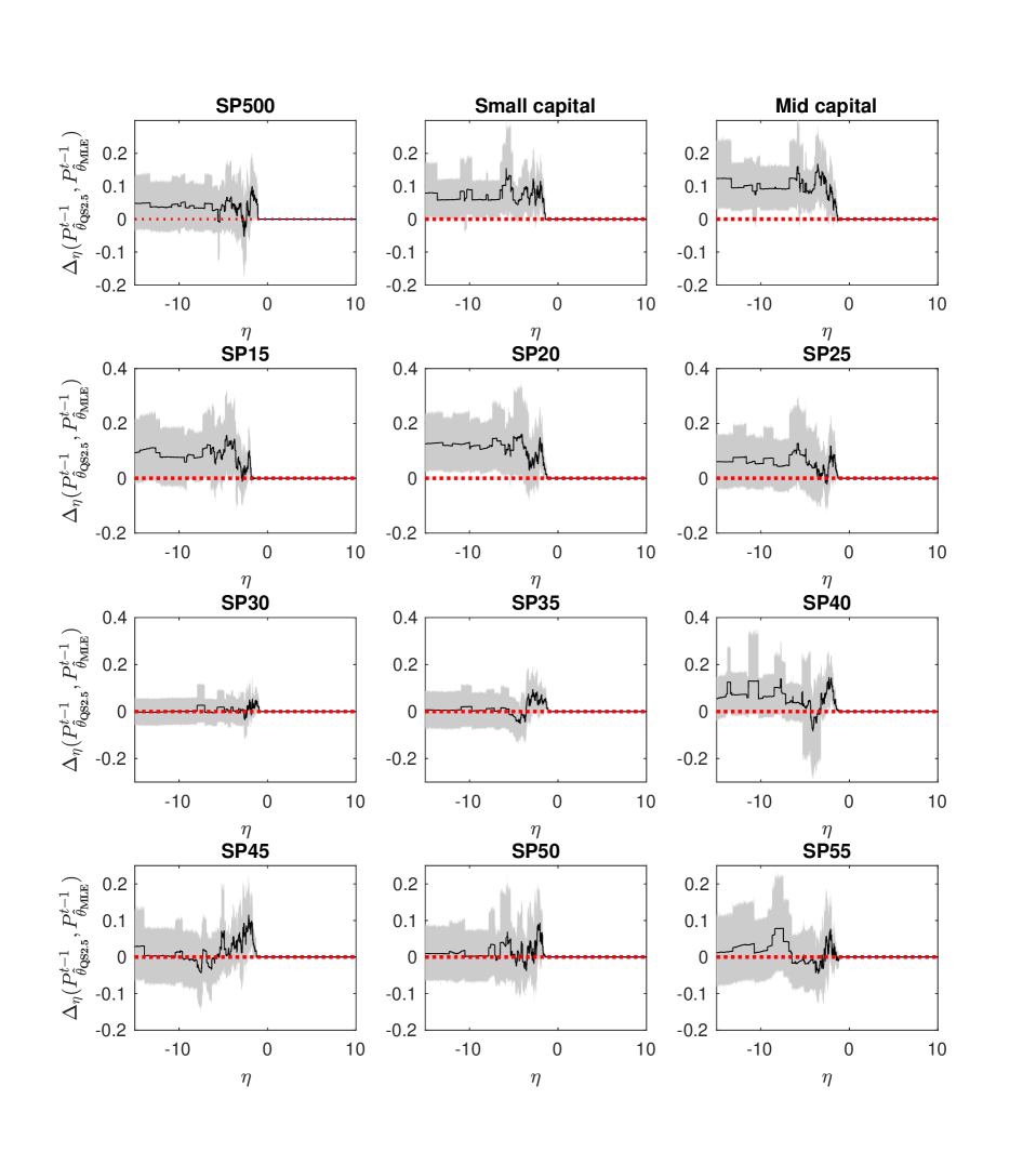
Figure 3: 2.5% ES performance for the 12 S&P indices using the Gaussian GARCH(1,1) as the predictive model. All Murphy diagrams depict $\Delta_{\eta}\left(P_{\boldsymbol{\hat{\theta}_{QS2.5}}}^{t-1},P_{\boldsymbol{\hat{\theta}_{MLE}}}^{t-1}\right)$, with the shaded area being the 95% bootstrapped confidence interval.

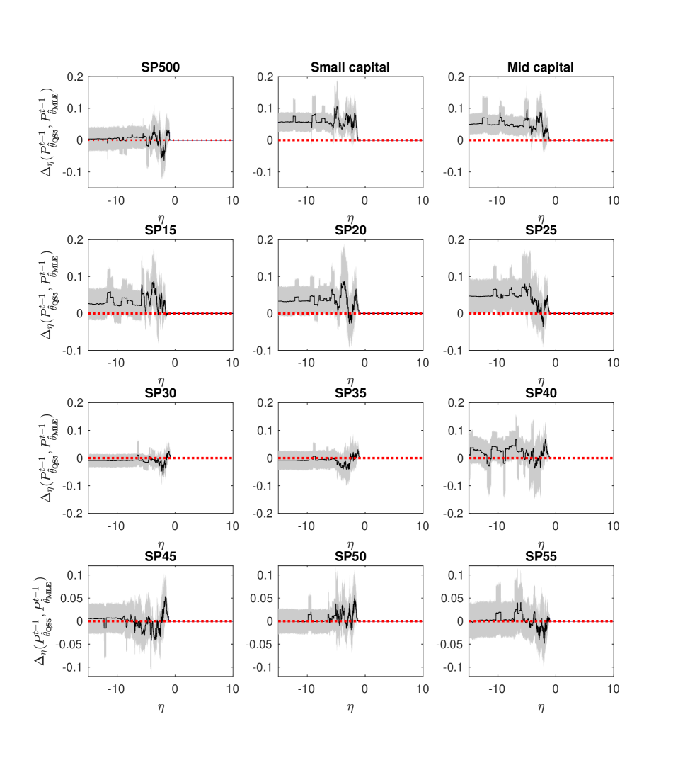
Figure 4: 5% ES performance for the 12 S&P indices using the Gaussian GARCH(1,1) as the predictive model. All Murphy diagrams depict $\Delta_{\eta}\left(P_{\boldsymbol{\hat{\theta}_{QS5}}}^{t-1},P_{\boldsymbol{\hat{\theta}_{MLE}}}^{t-1}\right)$, with the shaded area being the 95% bootstrapped confidence interval.

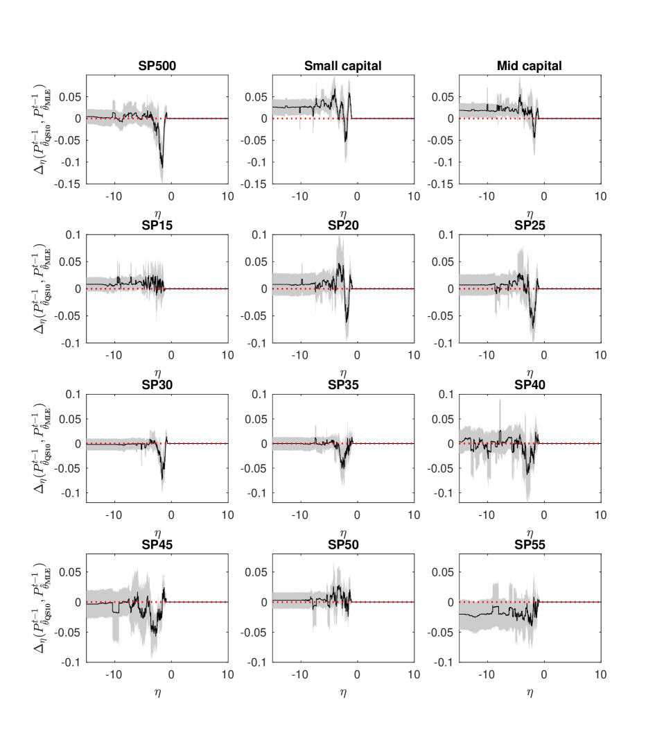
Figure 5: 10% ES performance for the 12 S&P indices using the Gaussian GARCH(1,1) as the predictive model. All Murphy diagrams depict $\Delta_{\eta}\left(P^{t-1}_{\boldsymbol{\hat{\theta}_{QS10}}},P^{t-1}_{\boldsymbol{\hat{\theta}_{MLE}}}\right)$, with the shaded area being the 95% bootstrapped confidence interval.

5 Optimizing the Predictive VIX Distribution for Dynamic Risk Management

The VIX is a volatility index published by the Chicago Board of Exchange (CBOE), and is a measure of US market volatility constructed from option prices. It is well known that the VIX index is negatively correlated with the stock market index, with the VIX typically rising in periods of market stress when there is a general decline in the stock market index. Such negative correlation is also observed between the stock index and the tradable futures contract written on the VIX index, with the correlation reportedly being stronger in the futures market (Moran and Liu,, 2020). As such, VIX futures contracts are often used as a tool to hedge against market downturns. In this section, we illustrate the benefits of optimizing the predictive distribution of the VIX index for the purpose of improving risk management strategies that involve a position in VIX futures.

5.1 The Predictive Model for the VIX index

The VIX index is a model-free measure of option implied volatility, extracted from options written on the S&P500 stock market index (see CBOE,, 2021, for more details). In theory, the VIX index measures the risk-neutral forward-looking expectation of the integrated variance of the underlying asset (see Britten-Jones and Neuberger,, 2000, and Jiang and Tian,, 2005). Thus, the movement in the VIX index not only closely tracks volatility itself, but also contains information about the forward-looking expectations of derivative traders, and is often viewed as a leading indicator of market movements as a result.

We have collected daily VIX index data from Yahoo Finance for the period: 27th September 1996 to 30th July 2020. The descriptive statistics of $\log(VIX_{t})$ are shown in Table 6. The statistics indicate that the marginal density of $\log(VIX_{t})$ is positively skewed and far from being normally distributed. As is typical with volatility measures, the VIX index has strong persistence, with its autocorrelation function remaining high in magnitude and statistically significant as the lag increases (with 20 lags being used for the Ljung-Box test of autocorrelation in Table 6).

Table 6: Descriptive statistics for the logarithm of the VIX volatility index. The Min and Max are the smallest and largest value of the sample series, respectively. Skewness is a measure of the asymmetry and kurtosis is a measure of fat tails with the normal distribution having a kurtosis equal to three. ‘JB.Test’ is the test statistic for the Jarque-Bera test of normality and the p-value is recorded in the table. ‘LB.Test’ is the test of serial correlation of the squared volatility based on 20 lags and the p-value is recorded in the table.

Series	Min	Median	Mean	Max	Skewness	Kurtosis	JB.Test	LB.Test
Log(VIX)	2.213	2.916	2.936	4.415	0.604	3.363	0.000	0.000

In order to capture the long memory feature of the VIX index, we employ the heterogeneous autoregressive (HAR) model to construct the predictive distribution of the VIX index. Proposed by Corsi, (2009), the HAR model is a simple additive linear model that uses moving averages of lagged values of the relevant dependent variable as regressors. It does not belong to the class of long memory models, but it is able to produce persistence that is almost indistinguishable from what is observed in financial volatility in practice, through the simple autoregressive-type structure. The HAR model and its extensions have been employed by previous studies on the predictability of the VIX index; see, for example, Maneesoonthorn et al., (2012) and Fernandes et al., (2014). We include a GARCH component in the HAR model to account for time variation in the second moment of the VIX distribution. The HAR-GARCH model is defined as:

$$\log(VIX_{t+1})=\beta_{0}+\beta_{1}\log(VIX_{t})+\beta_{2}\log(VIX_{t-5,t})+\beta_{3}\log(VIX_{t-22,t})+\sigma_{t+1}z_{t+1}$$ (11)

where

$$\sigma_{t+1}^{2}=\alpha_{0}+\alpha_{1}(\sigma_{t}z_{t})^{2}+\alpha_{2}\sigma_{t}^{2},$$ (12)

$$z_{t+1}\sim i.i.d.N(0,1)$$ (13)

and

$$\log(VIX_{t-m,t})=\frac{1}{m}\sum_{i=1}^{m}\log(VIX_{t+i-1}).$$ (14)

5.2 Performance of Optimal Prediction of the VIX Index

Using a similar expanding window predictive assessment procedure to that conducted in Sections 3.1 and 4.2, with an initial sample size equal to 1000 and out-of-sample size $\tau=T-1000=5000$, we produce and evaluate predictive densities based on the HAR-GARCH as defined in (11) to (14). We optimize the predictive distribution using the LS and the CLS scores corresponding to the 10% and 20% lower-tail, as well as the 80% and the 90% upper-tail of the marginal VIX distribution. Evaluation of out-of-sample performance uses this same set of scores.

Table 7 documents the average out-of-sample scores for the MLE-based and optimal predictives. Once again, bolded values represent the larger out-of-sample average score in a given column, with an asterisk denoting a case where the difference between the MLE and optimal predictive scores is significantly different from zero according to the test of Giacomini and White, (2006). The results from this table show that the optimal forecasts generate larger out-of-sample average scores in all cases (other than when the MLE and optimal predictives coincide), with the improvement statistically significant in the case of the CLS10 predictive.

Table 7: Average out-of-sample scores for prediction of the VIX index where the predictive model is the HAR-GARCH model with a Gaussian error. The model is calibrated using the LS (denoted by “MLE”), as well as the CLS in the column heading (denoted by “Optimal”). The column headings indicate the scores used to evaluate the out-of-sample performance of the probabilistic forecasts. The bolded value in a given column indicates the predictive (MLE-based or optimal) that generates the higher average score over the out-of-sample period, with an asterisk denoting rejection (at the 5% significance level) of the the null hypothesis of equal predictive ability according to the test of Giacomini and White, (2006).

Optimizers	Average out-of-sample scores
	LS	CLS10	CLS20	CLS80	CLS90
MLE	1.302	0.344	0.566	0.131	0.059
Optimal	1.302	0.350*	0.569	0.134	0.061

5.3 Application to Dynamic Risk Management with VIX Futures

Moran and Liu, (2020) demonstrate how VIX futures can be used for dynamic risk management. They outline a backtesting strategy that involves the static allocation of a 95% long position in the stock portfolio and a 5% long position in VIX futures. Since the VIX futures derive their value from the spot VIX index, they also propose a dynamic allocation strategy where the position in the VIX futures depends on the level of the spot VIX index itself.

To illustrate the possible benefit of score-based calibration in such a setting, we adapt the dynamic strategy illustrated in Moran and Liu, (2020) to incorporate the predictive distribution for the VIX index based on the HAR-GARCH model, but optimized using an appropriate version of the tail-focused CLS. We design two dynamic trading strategies, in which the position on the shortest maturity VIX future is triggered by one of two decision rules based on the optimal predictive for the VIX index. The opening and closing prices of the VIX futures contracts over the period between 24 September 2008 and 28 May 2021 are obtained directly from the CBOE website.

First, we backtest a predictive probability rule, where the 5% long position in the VIX futures is taken only if $\text{Pr}(VIX_{t+1}>VIX_{t}|\mathcal{F}_{t})>0.5$. That is, when the VIX index is likely to increase over the next day, we take a long position in the VIX futures in order to offset the potential fall that is expected in the stock market. To implement the predictive probability rule, we optimize the VIX predictive distribution according to the upper-tail CLS associated with the region where $VIX_{t}>VIX_{t-1}$, denoted by CLS($VIX_{t}>VIX_{t-1}$).

Second, we utilize the $80^{th}$ predictive VIX percentile to form a trading rule. Under this rule, the 5% long position in the VIX futures market is only undertaken if the $80^{th}$ predictive percentile of the spot VIX is greater than 40%. That is, the value that defines the upper 20% of the predictive distribution of the VIX must be high enough for the investor to take a position to offset the potential fall in the stock market. To implement this rule, the predictive distribution of the VIX is optimized according to CLS80.

Under both dynamic settings, the decision to adopt the VIX futures position is made at the beginning of the trading day, based on the relevant predictive distribution constructed from data up to the previous trading day. If a decision is made to enter a position in the VIX futures, a long position in the shortest maturity VIX futures contract is taken. The VIX futures position is closed off at day end, with the investor realizing the return that reflects the change from the opening price to the closing price of the VIX futures on that trading day.

Table 8 reports portfolio performance measures based on each of the dynamic strategies outlined above. The performance of the static portfolio, comprising a 95% long position in the S&P500 market portfolio and a 5% long position in the shortest maturity VIX futures, as in Moran and Liu, (2020), is also reported for comparison. For each dynamic strategy, we also produce results using the predictive distribution based on the MLE, for comparison. We report the mean excess return, that is, the portfolio return over and above the risk-free rate of return, the portfolio standard deviation, as well as the Sharpe ratio.

Under both dynamic trading rules, the predictive distributions constructed from the upper-tail CLS generate notably larger Sharpe ratios than do the MLE predictives, implying that the strategy undertaken with upper-tail calibration generates the greatest return relative to the risk undertaken. This observation confirms the need – in an empirical setting like this, in which the model misspecification prevails – to construct the predictive distribution that is optimal to the region of interest, in this case in the upper tail of the predictive VIX distribution. We also observe that the predictive percentile rule performs better than the predictive probability rule – for both forms of predictive. In fact, the portfolio constructed using the predictive probability rule and exploiting the MLE-based predictive performs worse than the static portfolio. This highlights the importance of region-specific calibration in rendering the dynamic risk management strategies unambiguously preferable to the simpler static option.

Table 8: Stock and VIX futures portfolio performance based on dynamic trading strategies. The results for the static portfolio made up of 95% S&P500 market portfolio and 5% VIX futures on all days, are also reported for comparison.

	Mean Ex. Returns	Std. Dev.	Sharpe Ratio
Static Portfolio	0.040	0.182	0.219
	Predictive probability rule
Optimizer
CLS($VIX_{t}>VIX_{t-1}$)	0.066	0.207	0.318
MLE	0.042	0.204	0.206
	$80^{th}$ Predictive percentile rule
Optimizer
CLS80	0.076	0.199	0.381
MLE	0.075	0.200	0.375

6 Conclusion

In this paper, we investigate the use of tail-focused optimal forecasts in the context of financial risk management. From both the simulation and empirical results, we establish the benefits of optimal forecasts in misspecified models, subject to the assumed predictive model being broadly suitable for modelling the data at hand. Focusing on the tail performance of optimal forecasts, the simulation results show that the more misspecified the model is, the more benefits can be gained from using the optimal forecasts, in comparison with adopting the conventional MLE-based forecasts. In particular, the gain from using optimal forecasts is more stark in the case of a skewed DGP, than in the case of fat-tailed DGP, when the assumed predictive model is conditionally Gaussian. We also establish that when tail risk is of interest, the optimal forecasts constructed from the quantile score yield better predictions than other alternatives in the context of value-at-risk coverage and expected shortfall accuracy.

The empirical analysis of 12 S&P indices confirms the qualitative nature of our simulation results. We also investigate the use of optimal forecasting in the context of VIX prediction, with a specific application to hedging stock market risk with VIX derivatives. Trading strategies constructed from tail-focused optimal forecasts are backtested, alongside trading strategies constructed from MLE-based forecasts, with the tail-focused forecasts generating substantially better return-risk tradeoffs in this context.

References

- Aastveit et al., (2018) Aastveit, K. A., Mitchell, J., Ravazzolo, F., and Van Dijk, H. K. (2018). The evolution of forecast density combinations in economics. Technical report, Tinbergen Institute Discussion Paper.
- Acerbi and Tasche, (2002) Acerbi, C. and Tasche, D. (2002). On the coherence of expected shortfall. Journal of Banking & Finance, 26(7):1487–1503.
- Bao et al., (2006) Bao, Y., Lee, T.-H., and Saltoglu, B. (2006). Evaluating predictive performance of value-at-risk models in emerging markets: a reality check. Journal of Forecasting, 25(2):101–128.
- BenSaïda et al., (2018) BenSaïda, A., Boubaker, S., Nguyen, D. K., and Slim, S. (2018). Value-at-risk under market shifts through highly flexible models. Journal of Forecasting, 37(8):790–804.
- Bollerslev, (1987) Bollerslev, T. (1987). A conditionally heteroskedastic time series model for speculative prices and rates of return. The Review of Economics and Statistics, pages 542–547.
- Borowska et al., (2020) Borowska, A., Hoogerheide, L., Koopman, S. J., and van Dijk, H. K. (2020). Partially censored posterior for robust and efficient risk evaluation. Journal of Econometrics, 217(2):335–355.
- Britten-Jones and Neuberger, (2000) Britten-Jones, M. and Neuberger, A. (2000). Option prices, implied price processes, and stochastic volatility. The Journal of Finance, 55(2):839–866.
- Brooks et al., (2005) Brooks, C., Clare, A., Dalle Molle, J. W., and Persand, G. (2005). A comparison of extreme value theory approaches for determining value at risk. Journal of Empirical Finance, 12(2):339–352.
- CBOE, (2021) CBOE (2021). Cboe volatility index. White Paper, pages 1–20.
- Chen et al., (2008) Chen, Y., Härdle, W., and Jeong, S.-O. (2008). Nonparametric risk management with generalized hyperbolic distributions. Journal of the American Statistical Association, 103(483):910–923.
- Chiang et al., (2021) Chiang, I.-H. E., Liao, Y., and Zhou, Q. (2021). Modeling the cross-section of stock returns using sensible models in a model pool. Journal of Empirical Finance, 60:56–73.
- Christoffersen, (1998) Christoffersen, P. F. (1998). Evaluating interval forecasts. International Economic Review, pages 841–862.
- Corsi, (2009) Corsi, F. (2009). A simple approximate long-memory model of realized volatility. Journal of Financial Econometrics, 7(2):174–196.
- Diks et al., (2011) Diks, C., Panchenko, V., and Van Dijk, D. (2011). Likelihood-based scoring rules for comparing density forecasts in tails. Journal of Econometrics, 163(2):215–230.
- Ding et al., (1993) Ding, Z., Granger, C. W., and Engle, R. F. (1993). A long memory property of stock market returns and a new model. Journal of Empirical Finance, 1(1):83–106.
- Ehm et al., (2016) Ehm, W., Gneiting, T., Jordan, A., and Krüger, F. (2016). Of quantiles and expectiles: consistent scoring functions, choquet representations and forecast rankings. Journal of the Royal Statistical Society: Series B (Statistical Methodology), 78(3):505–562.
- Engle and Manganelli, (2004) Engle, R. F. and Manganelli, S. (2004). CAViaR: Conditional autoregressive value at risk by regression quantiles. Journal of Business & Economic Statistics, 22(4):367–381.
- Fernandes et al., (2014) Fernandes, M., Medeiros, M. C., and Scharth, M. (2014). Modeling and predicting the CBOE market volatility index. Journal of Banking & Finance, 40:1–10.
- Fissler et al., (2015) Fissler, T., Ziegel, J. F., and Gneiting, T. (2015). Expected shortfall is jointly elicitable with value at risk-implications for backtesting. arXiv preprint arXiv:1507.00244.
- Gatarek et al., (2014) Gatarek, L., Hoogerheide, L., Hooning, K., van Dijk, H. K., et al. (2014). Censored posterior and predictive likelihood in left-tail prediction for accurate value at risk estimation. Technical report, Tinbergen Institute.
- Giacomini and Komunjer, (2005) Giacomini, R. and Komunjer, I. (2005). Evaluation and combination of conditional quantile forecasts. Journal of Business & Economic Statistics, 23(4):416–431.
- Giacomini and White, (2006) Giacomini, R. and White, H. (2006). Tests of conditional predictive ability. Econometrica, 74(6):1545–1578.
- Gneiting, (2011) Gneiting, T. (2011). Making and evaluating point forecasts. Journal of the American Statistical Association, 106(494):746–762.
- Gneiting and Raftery, (2007) Gneiting, T. and Raftery, A. E. (2007). Strictly proper scoring rules, prediction, and estimation. Journal of the American statistical Association, 102(477):359–378.
- Gneiting et al., (2005) Gneiting, T., Raftery, A. E., Westveld III, A. H., and Goldman, T. (2005). Calibrated probabilistic forecasting using ensemble model output statistics and minimum CRPS estimation. Monthly Weather Review, 133(5):1098–1118.
- Hansen et al., (2012) Hansen, P. R., Huang, Z., and Shek, H. H. (2012). Realized GARCH: a joint model for returns and realized measures of volatility. Journal of Applied Econometrics, 27(6):877–906.
- Jensen and Maheu, (2013) Jensen, M. J. and Maheu, J. M. (2013). Bayesian semiparametric multivariate GARCH modeling. Journal of Econometrics, 176(1):3–17.
- Jiang and Tian, (2005) Jiang, G. J. and Tian, Y. S. (2005). The model-free implied volatility and its information content. The Review of Financial Studies, 18(4):1305–1342.
- Koenker and Bassett, (1978) Koenker, R. and Bassett, G. (1978). Regression quantiles. Econometrica, pages 33–50.
- Konstantinidi et al., (2008) Konstantinidi, E., Skiadopoulos, G., and Tzagkaraki, E. (2008). Can the evolution of implied volatility be forecasted? Evidence from European and US implied volatility indices. Journal of Banking & Finance, 32(11):2401–2411.
- Laporta et al., (2018) Laporta, A. G., Merlo, L., and Petrella, L. (2018). Selection of value at risk models for energy commodities. Energy Economics, 74:628–643.
- Loaiza-Maya et al., (2021) Loaiza-Maya, R., Martin, G. M., and Frazier, D. T. (2021). Focused bayesian prediction. Journal of Applied Econometrics, 36(5):517–543.
- Maheu and McCurdy, (2004) Maheu, J. M. and McCurdy, T. H. (2004). News arrival, jump dynamics, and volatility components for individual stock returns. The Journal of Finance, 59(2):755–793.
- Maneesoonthorn et al., (2017) Maneesoonthorn, W., Forbes, C. S., and Martin, G. M. (2017). Inference on self-exciting jumps in prices and volatility using high-frequency measures. Journal of Applied Econometrics, 32(3):504–532.
- Maneesoonthorn et al., (2012) Maneesoonthorn, W., Martin, G. M., Forbes, C. S., and Grose, S. D. (2012). Probabilistic forecasts of volatility and its risk premia. Journal of Econometrics, 171(2):217–236.
- Martin et al., (2022) Martin, G. M., Loaiza-Maya, R., Maneesoonthorn, W., Frazier, D. T., and Ramírez-Hassan, A. (2022). Optimal probabilistic forecasts: When do they work? International Journal of Forecasting, 38(1):384–406.
- Moran and Liu, (2020) Moran, M. T. and Liu, B. (2020). The VIX Index and Volatility-Based Global Indexes and Trading Instruments: A Guide to Investment and Trading Features. CFA Institute Research Foundation.
- Opschoor et al., (2017) Opschoor, A., Van Dijk, D., and van der Wel, M. (2017). Combining density forecasts using focused scoring rules. Journal of Applied Econometrics, 32(7):1298–1313.
- Patton, (2019) Patton, A. J. (2019). Comparing possibly misspecified forecasts. Journal of Business & Economic Statistics, pages 1–23.
- Smith and Maneesoonthorn, (2018) Smith, M. S. and Maneesoonthorn, W. (2018). Inversion copulas from nonlinear state space models with an application to inflation forecasting. International Journal of Forecasting, 34(3):389–407.
- Tasche, (2002) Tasche, D. (2002). Expected shortfall and beyond. Journal of Banking & Finance, 26(7):1519–1533.
- Taylor, (2019) Taylor, N. (2019). Forecasting returns in the VIX futures market. International Journal of Forecasting, 35(4):1193–1210.
- Wang et al., (2022) Wang, X., Hyndman, R. J., Li, F., and Kang, Y. (2022). Forecast combinations: an over 50-year review. International Journal of Forecasting.
- Yamai and Yoshiba, (2005) Yamai, Y. and Yoshiba, T. (2005). Value-at-risk versus expected shortfall: A practical perspective. Journal of Banking & Finance, 29(4):997–1015.
- Ziegel et al., (2020) Ziegel, J. F., Krüger, F., Jordan, A., and Fasciati, F. (2020). Robust forecast evaluation of expected shortfall. Journal of Financial Econometrics, 18(1):95–120.