Fundamental Bound on Epidemic Overshoot in the SIR Model

Abstract

We derive an exact upper bound on the epidemic overshoot for the Kermack-McKendrick SIR model. This maximal overshoot value of 0.2984… occurs at $R_{0}^{*}$ = 2.151… . In considering the utility of the notion of overshoot, a rudimentary analysis of data from the first wave of the COVID-19 pandemic in Manaus, Brazil highlights the public health hazard posed by overshoot for epidemics with $R_{0}$ near 2. Using the general analysis framework presented within, we then consider more complex SIR models that incorporate vaccination.

Introduction

The overshoot of an epidemic is the proportion of the population that becomes infected after the peak of the epidemic has already passed. Formally, it is given as the difference between the fraction of the population that is susceptible at the peak of infection prevalence and at the end of the epidemic. Intuitively, it is the difference between the herd immunity threshold and the total fraction of the population that gets infected [1, 2]. As it describes the damage to the population in the declining phase of the epidemic (i.e. when the effective reproduction number is less than 1), one might be tempted to dismiss its relative importance. However, a substantial proportion of the epidemic, and thus a large number of people, may be impacted during this phase of the epidemic dynamics.

A natural question to ask then is how large can the overshoot be and how does the overshoot depend on epidemic parameters, such as transmissibility and recovery rate? Surprisingly, this question can be answered exactly. In this paper, we first derive the bound on the overshoot in the Kermack-McKendrick limit of the SIR model [3]. We then compare the predictions of this feature of the SIR model with data taken from the first wave of the COVID-19 pandemic in Manaus, Brazil ([4]). Beyond the basic SIR model, we then see if the bound on overshoot holds if we add additional complexity, such as vaccinations.

Results

Over the years, the Kermack-McKendrick SIR model has become largely synonymous with the following set of ordinary differential equations (ODEs) due to their simplicity and popularity:

$$\frac{dS}{dt} =-\beta SI$$ (1)

$$\frac{dI}{dt} =\beta SI-\gamma I$$ (2)

$$\frac{dR}{dt} =\gamma I$$ (3)

where $S,I$, and $R$ are the fractions of population in the susceptible, infected, or recovered state respectively. As these are the only possible states within this model, the conservation equation for the whole population is given as $S+I+R=1$. It is worth noting that the original compartmental model formulated by Kermack and McKendrick in their seminal paper from a century ago [3] is actually a more general model than the ODE model that has become synonymous with their names. The original model considered both infectiousness that depended on the amount of time since becoming infected, which has been termed age of infection, and demographic effects in the form of deaths. A considerable amount has been learned and understood in the case of the more general model that considers age of infection (see [5, 6] for an introduction), which typically takes the form of a nonlinear renewal equation. While here we have chosen to focus on the simpler ODE model, under certain assumptions our result for the overshoot can be carried over to the age-of-infection model as well.

Conceptually, the overshoot can be equivalently calculated in two ways. In the first it is given by the difference in the fraction of susceptible individuals at the peak of infection prevalence ($S_{t_{*}}$) and at the end of the end of the epidemic ($S_{\infty}$) (Figure 1a). Alternatively, it can be viewed as the integration of the number of newly infected individuals, which is given by the infection incidence rate ($\beta SI$) from the peak of infection prevalence to the end of the epidemic (Figure 1b). We will make use of the former relationship in the results that follow.

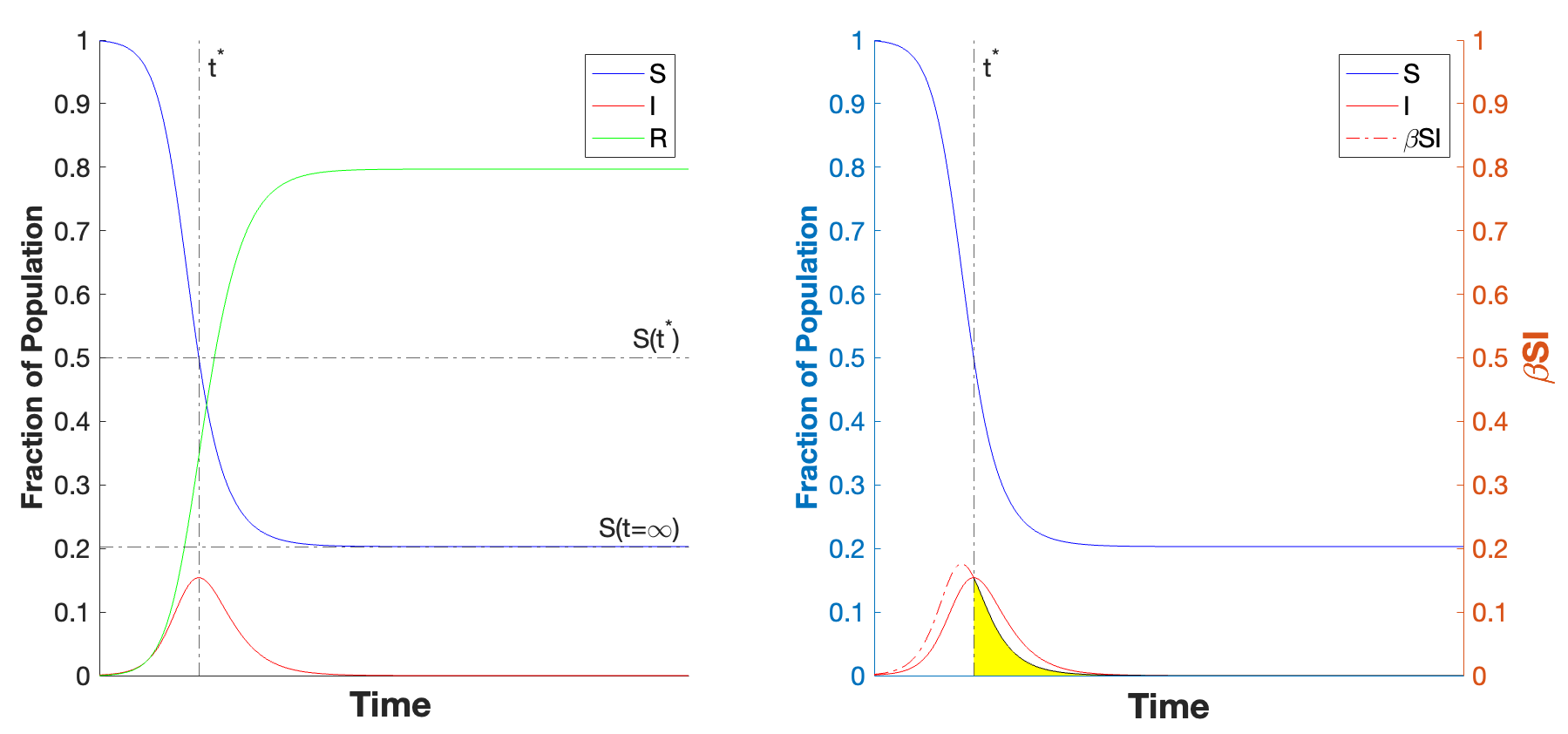
Figure 1: The overshoot can be calculated in two ways: a) Overshoot is calculated as the difference between the fraction of the population that is susceptible at $t^{*}$ and infinite time. b) Overshoot is calculated as the integral of the infection incidence curve from $t^{*}$ until infinite time. Therefore overshoot corresponds to the area of the region shaded in yellow.

The only two parameters of the ODE model are $\beta$ and $\gamma$. A key parameter in epidemic modeling combines these two into a single parameter by taking their ratio, which is known as the basic reproduction number ($R_{0}$). The behavior of the overshoot can be shown to be only dependent on this single parameter, $R_{0}$. Plotting the dependency of overshoot on $R_{0}$ (Figure 2), we observe a peak in the curve at ($R_{0}^{*},Overshoot^{*}$) that sets an upper bound on the overshoot. From a public health perspective, diseases that have estimated $R_{0}$’s near this peak region in Figure 2 include COVID-19 (ancestral strain) [7], SARS [8], diphtheria [9], monkeypox [10], and ebola [11]. This peak phenomena in the overshoot was first numerically observed by [12], though not explained. We will now derive the solution for this maximum point analytically.

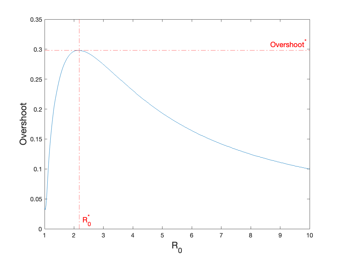
Figure 2: The overshoot as a function of $R_{0}$ for the Kermack-McKendrick SIR model.

Deriving the Exact Bound on Overshoot in the Kermack-McKendrick SIR Model

Theorem: The maximum possible overshoot in the Kermack-McKendrick SIR model is a fraction $0.2984...$ of the entire population, with a corresponding $R_{0}^{*}=2.151...$.

Proof.
Let $t^{*}$ be the time at the peak of the infection prevalence curve. Here we define the herd immunity threshold as the difference in the fractions of the population that are susceptible at zero time and at $t^{*}$. Then, the overshoot is defined as the difference in the fractions of the population that are susceptible at $t^{*}$ and at infinite time. This is equivalent to defining overshoot as the cumulative fraction of the population that gets infected after $t^{*}$.

$$Overshoot \equiv\int_{t^{*}}^{\infty}-(\frac{dS}{dt})\,dt=\int_{t*}^{\infty}\beta SI\,dt$$

$$=S_{t*}-S_{\infty}$$ (4)

where $S_{t*}$ and $S_{\infty}$ are the susceptible fractions at $t^{*}$ and infinite time respectively. We will use $S_{t*}=\frac{1}{R_{0}}$ [13], which can be obtained by setting (2) to zero and solving for that critical $S$. We will use the notation $X_{t}$ to indicate the value of compartment X at time $t$.

$$Overshoot=\frac{1}{R_{0}}-S_{\infty}$$ (5)

It is worth noting that the result that follows also holds for the more general age-of-infection model [3] if we restrict our definition of the herd immunity threshold to be the fraction of people that need to be removed from the population at the beginning of the epidemic to prevent an outbreak from occurring. While this alternative definition gives an equivalent herd immunity threshold in the ODE model where it is defined in terms of the peak of the prevalence curve, this more robust definition is needed to account for the more complicated behavior in the age-of-infection model.

Since we would like to compute maximal overshoot, we can differentiate the overshoot equation (5) with respect to $S_{\infty}$ to find the extremum. We will eliminate $R_{0}$ from the overshoot equation so that we have an equation only in terms of $S_{\infty}$.

To find an expression for $R_{0}$, we start by deriving the standard final size relation for the SIR model [14, 15]. We solve for the rate of change of I as a function of S using (1)-(2) to obtain

$${\frac{dI}{dS}} =-1+\frac{\gamma}{\beta S}$$

from which it follows on integration that $S+I-\frac{\gamma}{\beta}\ln S$ is constant along any trajectory.

Considering the beginning of the epidemic and the peak of the epidemic yields:

$$S_{0}+I_{0}-\frac{\gamma}{\beta}\ln S_{0} =S_{\infty}+I_{\infty}-\frac{\gamma}{\beta}\ln S_{\infty}$$

hence

$$\frac{\beta}{\gamma}(S_{\infty}-S_{0}+I_{\infty}-I_{0}) =\ln(\frac{S_{\infty}}{S_{0}})$$ (6)

We now define the initial conditions: $S_{0}=1-\epsilon$ and $I_{0}=\epsilon$, where $\epsilon$ is the (infinitesimally small) fraction of initially infected individuals. We assume that the number of initially infected individuals ($\epsilon$) is much smaller than the size of the population (i.e., $\epsilon<<1$). For the scale that we have in mind, such as those of city populations and larger, it is thus reasonable to make the approximation $1-\epsilon\approx 1$. We also use the standard asymptotic of the SIR model that there are no infected individuals at the end of an SIR epidemic: $I_{\infty}=0$. Taking the above conditions together and recalling that $R_{0}=\frac{\beta}{\gamma}$, we obtain that

$$S_{\infty} =e^{R_{0}(S_{\infty}-1)}$$ (7)

The resulting equation (7) is the final size relation for the Kermack-McKendrick SIR model. Importantly, this final size relation taken together with the alternative definition for the herd immunity threshold implies the subsequent result for overshoot holds not only for the simpler ODE model considered here, but also for the more general age-of-infection model of Kermack and McKendrick [3]. The robustness of the final size relation in the context of the more general model can be more easily viewed through the lens of a renewal equation for the force of infection, see [16, 6, 17, 15] for a derivation and a more complete discussion.

Rearranging for $R_{0}$ yields the following expression:

$$\frac{\ln(S_{\infty})}{S_{\infty}-1} =R_{0}$$ (8)

We then substitute this $R_{0}$ expression (8) into the overshoot equation (5).

$$Overshoot=\frac{S_{\infty}-1}{\ln(S_{\infty})}-S_{\infty}$$ (9)

Differentiating with respect to $S_{\infty}$ and setting the equation to zero to find the maximum overshoot yields:

$$(\ln S_{\infty*})^{2}=\ln S_{\infty*}-1+\frac{1}{S_{\infty*}}$$ (10)

whose solution is

$$S_{\infty*}=0.1664...$$

and which corresponds to

$$Overshoot^{*} =0.2984...$$ (11)

using (9). The corresponding $R_{0}$ calculated using (8) is

$$R_{0}^{*} =2.151...$$ (12)

This concludes the proof $\blacksquare$

Additionally, to find the total recovered fraction is straightforward. In the asymptotic limit of the SIR model, there are no remaining infected individuals, so $R_{\infty*}=1-S_{\infty*}$.

$$R_{\infty*}=1-0.1664...=0.8336...$$ (13)

In other words, approximately 5 out of every 6 individuals in the population will have experience infection when overshoot is maximized.

Discussion

We have proved that the maximum fraction of the population that can be infected during the overshoot phase of an epidemic in the Kermack-McKendrick SIR model is just under $0.3$, with a corresponding basic reproduction number of $R_{0}\approx 2.15$.

Given the clear predictions of this feature of the SIR model, it is reasonable to ask whether the theory matches any real-world epidemics. While high-quality data on large, unmitigated epidemics (for which the SIR model would most directly apply) in human populations is rare, we will now perform a rudimentary analysis of data from the first wave of the COVID-19 pandemic in Manaus, Brazil as given by Buss et al. ([4]). While the city did implement some small level of non-pharmaceutical interventions, for the purpose of calculation let us take at face value that the epidemic spread through the city practically unmitigated.

To estimate the theoretical prediction of overshoot in the SIR model, we need to first estimate $R_{0}$. The conservative, forward-looking approach we take here is to take the maximum of the effective reproduction number ($R_{t}$) when the epidemic is first starting. Using data from Buss et al. for $R_{t}$ in Manaus as a function of date of symptom onset, which we take as a proxy for time ([4]), the $R_{0}$ was approximately 2.3 in Manaus in mid-March (Figure A1). For $R_{0}=2.3$, using Figure 2 as a reference, the theoretical prediction for overshoot is approximately $29\%$. Thus, if $R_{0}$ can be estimated early on in the epidemic, the overshoot can be subsequently predicted within the context of an SIR model before the peak of the epidemic occurs, which in practice provides more time for public health measures and interventions to be implemented before the overshoot phase takes place.

To calculate the overshoot as observed directly from the data, we again refer to the time series data for $R_{t}$ (Figure A1). We will consider the time when $R_{t}=1$ to be when the epidemic peaks ($t^{*}$). Reading the data suggests the first COVID-19 wave peaked in late April. We note that $R_{t}$ stays around 1 until mid-August, when it starts rising again. As the basic SIR model does not consider such complex late-time behavior, for the purpose of this analysis, we will consider the first wave to have ended by mid-August. We note that assigning an endpoint to the data is a strong assumption, and that actually determining the turning and end point of an epidemic in the context of epidemic forecasting is not a simple matter [18].

With the date of an epidemic peak in hand, we now turn to reading the prevalence curve. Specifically, we will be using the mean data given by seroreversion-adjusted prevalence at a 1.4 S/C threshold for positive detection (Figure A2), which is adapted from Buss et al. [4]. The seroreversion adjustment is their best attempt for controlling for antibody waning. Given this correction, we will take this curve as the cumulative outbreak size. The 1.4 S/C threshold is based on the sampling threshold in relative light units for deciding whether a sample has a significant positive chemiluminescence signal over the calibration. After fitting the time series points to a simple logistic curve, it can be seen that when $R_{t}$ first reached 1 (indicating the epidemic had peaked), the cumulative fraction of the population that had been infected was approximately $36\%$. From here, we see that the cumulative fraction that becomes infected between this time point when $R_{t}$ first reached 1 and the end of the first wave in mid-August (i.e. the overshoot) is $30\%$ from the data.

We therefore see that the SIR model prediction for overshoot aligns with the value derived from the data, suggesting that the dynamics of the first wave of COVID-19 in Manaus, Brazil can be approximated by a simple SIR model. While the crude analysis above makes several strong assumptions about the nature of the unmitigated spread, the endpoint of the wave, the accuracy of the seroprevalence testing and correction methods, and the fidelity of the sampling intervals, the fit between the data and a SIR model is perhaps unsurprising given the relatively high population density of Manaus and general lack of thorough mitigation measures. To a first-order approximation, the data suggests that overshoot indeed poses a significant amount of public health hazard when the $R_{0}$ is in the neighborhood of 2. And that for well-mixed, unmitigated epidemics that may be approximated by SIR dynamics, overshoot may be a sizeable portion of the dynamics and overall attack rate.

The mathematical intuition on why there is a peak in the overshoot as a function of $R_{0}$ can be seen by inspection of Equation 5. The first term, $\frac{1}{R_{0}}$, monotonically decreases with increasing $R_{0}$ . The last term, $-S_{\infty}$, monotonically increases with $R_{0}$. Thus a trade-off in the two terms results in a single intermediate peak. The epidemiological intuition behind a peak in the overshoot is that the total number of individuals infected during the epidemic grows monotonically with increasing $R_{0}$. However, too high of an $R_{0}$ leads to a sharp growth in the number of infected individuals, which burns through most of the population before the infection prevalence peak is reached, leaving few susceptible individuals left for the overshoot phase. This is seen by a monotonic decrease in the fraction of infected individuals that occur in the overshoot phase with increased $R_{0}$ (Figure A3). Thus the maximal overshoot occurs as a trade-off between those two directions. It is interesting to note that while the overshoot is a non-monotonic function of $R_{0}$, in contrast, the ratio of overshoot to outbreak size is a strictly decreasing function of $R_{0}$ (see Supplemental Information for further discussion).

The fundamental upper bound on the overshoot derived here also seems to hold under the addition of more complexity into the SIR model (see Supplemental Information). Upon the addition of different modes of vaccination, we find the bound on overshoot still holds in all cases considered. In the 2-strain with vaccination SIR model of Zarnitsyna et al. [12], the overshoot depends on both the level of strain dominance and vaccination rate, but from their results it is numerically seen that any amount of vaccination will produce an overshoot lower than the bound found here. Different control measures and strategies may reduce the overshoot as compared to the unmitigated case [1], keeping this upper bound intact. Future work may explore how general this bound is for SIR models with other types of complexities or for models beyond the SIR-type.

Author Contributions

M.M.N., A.S.F., S.A.O., S.A.L. designed research, performed research, and wrote and reviewed the manuscript.

Data Accessibility

Code to generate Results and Figures is given in the Supplemental Materials.

Funding Statement

The authors would like to acknowledge generous funding support provided by the National Science Foundation (CCF1917819 and CNS-2041952), the Army Research Office (W911NF-18-1-0325), and a gift from the William H. Miller III 2018 Trust. The authors declare no competing interests.

Supplemental Materials: Fundamental Bound on Epidemic Overshoot in the SIR Model

Upper Bounds on Overshoot in Models that Include Vaccinations

Beyond the Kermack-McKendrick SIR model, one can ask if the bound on overshoot still holds if other complexities are added to the model. First, we will consider the addition of vaccinations.

We will consider three qualitatively different types of curves for the vaccination rate (Figure A4). These correspond to different scenarios that might be modeled. The first model assumes a vaccination rate of zero after the outbreak begins, which implies all vaccinations occur before the outbreak. The second model of vaccination assumes a constant per-capita vaccination rate. This is a situation where all susceptible individuals get vaccinated at the same rate. This assumption yields a vaccination curve for the population that is concave down. The third type of model assumes a risk-driven vaccination rate that depends on the number of infected individuals. This yields a non-monotonic vaccination curve for the population that switches from being initially concave up to being concave down. Depending on the scenario being analyzed, one model might be more appropriate to use than others. Below we discuss each model in further detail by providing the corresponding system of equations, relevant scenarios the model might correspond to in reality, and the corresponding maximal overshoot for each model.

Maximal Overshoot when the Number of Vaccinated Individuals is Constant

The first model of vaccination assumes there are no vaccinations during the outbreak, which implies a fixed number of vaccinated individuals over the course of the epidemic. Such a scenario might be the reintroduction of an infectious disease into a population that has a pre-existing level of immunity.

Since the number of vaccinated individuals is constant, this implies all vaccinations occurred prior to the initial time step. The calculation is then trivial assuming vaccinations provide complete and permanent immunity. In that case, vaccinated individuals can simply be ignored entirely in the dynamics, resulting in the maximal overshoot simply scaling with the unvaccinated fraction.

$$Overshoot^{*}_{SIRV}=(1-V)0.2984...$$ (14)

Maximal Overshoot Under Addition of Constant Per-Capita Vaccination

We next consider a more typical scenario where the vaccination rate per unvaccinated individual is constant per unit time. Barring any additional information about the population or the epidemic, it is reasonable to assume that all susceptible individuals are vaccinated at the same rate. Consider the following SIRV model:

$$\frac{dS}{dt} =-\beta SI-\lambda S$$ (15)

$$\frac{dI}{dt} =\beta SI-\gamma I$$ (16)

$$\frac{dR}{dt} =\gamma I$$ (17)

$$\frac{dV}{dt} =\lambda S$$ (18)

In this case, it is easily shown that there is a conserved quantity, $S+I-\frac{\gamma}{\beta}\ln S+\frac{\lambda}{\beta}\ln I$, which reduces to (6) when the vaccination rate is zero (i.e. $\lambda=0$). Unfortunately, having the conserved quantity is not sufficient to compute the overshoot, since there does not appear to be a way to separate infected and vaccinated individuals when trying to extend the previous calculation. Therefore, we turn to numerical computation (Figure A5a). We find that the maximal overshoot is bounded above by the value already obtained in the model without vaccinations. As shown in Figure A5, the overshoot has a complicated dependence on the vaccination parameter $\lambda$ and $R_{0}$.

Maximal Overshoot Under Addition of a Risk-Driven Vaccination Rate

Lastly consider a vaccination rate that is proportional to the number of infected individuals. Such risk-driven behavior may arise for a variety of reasons, including initial vaccine hesitancy, a delay in vaccine availability, or a correlation between willingness to get vaccinated and the number of infected individuals. Consider the following SIRV model:

$$\frac{dS}{dt} =-\beta SI-\lambda SI$$ (19)

$$\frac{dI}{dt} =\beta SI-\gamma I$$ (20)

$$\frac{dR}{dt} =\gamma I$$ (21)

$$\frac{dV}{dt} =\lambda SI$$ (22)

Since the model now has an additional compartment, V, compared with the original SIR model, we must update our definition for overshoot accordingly. Fundamentally, overshoot compares the fraction of people who have not been infected at the epidemic peak and the people who have not been infected at the end of the epidemic. The fraction of people who have not been infected at any particular time, $t$, is $S_{t}+V_{t}$. Thus, overshoot can be redefined as follows.

$$Overshoot=(S_{t^{*}}+V_{t^{*}})-(S_{\infty}+V_{\infty})$$

Since the equation for $\frac{dI}{dt}$ remains unchanged, $S_{t^{*}}=\frac{1}{R_{0}}$ still applies. Thus, the overshoot equation for models with vaccinated compartments is given by:

$$Overshoot=(\frac{1}{R_{0}}+V_{t^{*}})-(S_{\infty}+V_{\infty})$$ (23)

To maximize overshoot, we thus need to find expressions for $R_{0},V_{t^{*}}$, and $V_{\infty}$ in terms of $S_{\infty}$.

To find $R_{0}$ we start by taking the ratio $\frac{dI}{dS}$ and integrating as before. It follows that $I+\frac{\beta}{\beta+\lambda}S-\frac{\gamma}{\beta+\lambda}\ln S$ is constant along any trajectory. Considering the beginning and the end of the epidemic yields:

$$I_{0}+\frac{\beta}{\beta+\lambda}S_{0}-\frac{\gamma}{\beta+\lambda}\ln S_{0} =I_{\infty}+\frac{\beta}{\beta+\lambda}S_{\infty}-\frac{\gamma}{\beta+\lambda}\ln S_{\infty}$$

Using the same initial conditions, asymptotic behavior, and parameter substitution as before ($S_{0}=1-\epsilon,I_{0}=\epsilon,I_{\infty}=0,R_{0}=\frac{\beta}{\gamma}$) yields the following final size relation.

$$R_{0} =\frac{\ln(S_{\infty})}{S_{\infty}-1}$$ (24)

Thus, we see that $R_{0}$ for this SIRV model takes on the same expression as the SIR model (8).

To find $V_{t^{*}}$, let us take the ratio of time derivatives of the S and V compartments (19), (22),

$$\frac{\frac{dS}{dt}}{\frac{dV}{dt}} =\frac{-\beta SI-\lambda SI}{\lambda SI}$$

$${\frac{dS}{dV}} =-(\frac{\beta+\lambda}{\lambda})$$

from which it follows on integration that $S+(\frac{\beta+\lambda}{\lambda})V$ is constant along any trajectory. Considering the beginning and the peak of the epidemic yields:

$$S_{0}+(\frac{\beta+\lambda}{\lambda})V_{0}=S_{t^{*}}+(\frac{\beta+\lambda}{\lambda})V_{t^{*}}$$

Using the initial conditions ($S_{0}=1-\epsilon,I_{0}=\epsilon,V_{0}=0$) and recalling that $S_{t^{*}}=\frac{1}{R_{0}}$, we obtain the following formula for $V_{t^{*}}$.

$$V_{t^{*}}=(1-\frac{1}{R_{0}})(\frac{\lambda}{\beta+\lambda})$$ (25)

To find $V_{\infty}$, recall that $S+(\frac{\beta+\lambda}{\lambda})V$ is constant along any trajectory. Considering the peak of the epidemic and the end of the epidemic yields

$$S_{t^{*}}+(\frac{\beta+\lambda}{\lambda})V_{t^{*}}=S_{\infty}+(\frac{\beta+\lambda}{\lambda})V_{\infty}$$

Using the equation for $V_{t^{*}}$ (25) and recalling that $S_{t^{*}}=\frac{1}{R_{0}}$, we obtain the following equation for $V_{\infty}$.

$$V_{\infty}=(1-S_{\infty})(\frac{\lambda}{\beta+\lambda})$$ (26)

Substituting the expressions for $R_{0}$ (24), $V_{t^{*}}$ (25), $V_{\infty}$ (26) into the overshoot equation (23) yields:

$$Overshoot =(\frac{S_{\infty}-1}{\ln(S_{\infty})}-S_{\infty})(1-\frac{\lambda}{\beta+\lambda})$$ (27)

We see that this expression for the overshoot is simply the overshoot expression for the original SIR model (9) scaled by a factor $1-\frac{\lambda}{\beta+\lambda}$.

$$Overshoot_{SIRV(\lambda SI)} =Overshoot_{SIR}(1-\frac{\lambda}{\beta+\lambda})$$ (28)

Since both $\beta,\lambda\geq 0$, then the factor $1-\frac{\lambda}{\beta+\lambda}$ can never be greater than 1. This implies that the bound on maximal overshoot given by the theorem holds, becoming exact in the limit of no vaccinations (ie. $\lambda=0$). For this model, the maximal overshoot decreases as a function of $\lambda$ in a nonlinear way and has a nonlinear dependence on $R_{0}$ (Figure A6).

The Ratio of Overshoot to Outbreak Size

In the main text, we consider the calculation of overshoot alone. It is also interesting to ask how the overshoot compares to the final attack rate given by the outbreak size. It turns out we can do the calculation analytically using the previous definition for $Overshoot=\frac{1}{R_{0}}-S_{\infty}$ (5) and defining the total outbreak size as $\textit{Outbreak Size}=1-S_{\infty}=R_{\infty}$.

Taking the ratio of the two definitions yields:

$$\frac{Overshoot}{\textit{Outbreak Size}}=\frac{\frac{1}{R_{0}}-S_{\infty}}{1-S_{\infty}}=\frac{1}{R_{0}(1-S_{\infty})}-\frac{S_{\infty}}{1-S_{\infty}}$$ (29)

Substituting $R_{0}$ using the relationship given by (8) yields:

$$\frac{Overshoot}{\textit{Outbreak Size}}=\frac{-1}{\ln S_{\infty}}-\frac{S_{\infty}}{1-S_{\infty}}$$ (30)

Differentiating this equation with respect to $S_{\infty}$ and setting it to zero to find the extremal points $S_{\infty}^{*}$ yields:

$$\frac{d(\frac{Overshoot}{\textit{Outbreak Size}})}{dS_{\infty}}=0=\frac{1}{S_{\infty}^{*}(\ln S_{\infty}^{*})^{2}}-\frac{1}{(1-S_{\infty}^{*})^{2}}$$ (31)

It can be seen upon inspection that the only real solution for $(1-S_{\infty}^{*})^{2}=S_{\infty}^{*}(\ln S_{\infty}^{*})^{2}$ is at the point $S_{\infty}^{*}=1.$ This only occurs in the limit of $R_{0}=1$. Thus, at $R_{0}$ = 1, the overshoot exactly equals the outbreak size. Then, the overshoot becomes a strictly decreasing fraction of the total outbreak size with increasing $R_{0}$.

It can be shown that the only real solution to $(1-S_{\infty}^{*})^{2}=S_{\infty}^{*}(\ln S_{\infty}^{*})^{2}$ for $0\leq S_{\infty}^{*}\leq 1$ is at the point $S_{\infty}^{*}=1.$

Since $S_{\infty}^{*}=0$ is clearly not a solution, we rule that out. Since $(1-S_{\infty}^{*})^{2}=S_{\infty}^{*}(\ln S_{\infty}^{*})^{2}$ at $S_{\infty}^{*}=1$, it suffices to show that $f(S_{\infty}^{*})\colon=(1-S_{\infty}^{*})^{2}-S_{\infty}^{*}(\ln S_{\infty}^{*})^{2}>0$ for all $0<S_{\infty}^{*}<1$. Since $f^{\prime}(S_{\infty}^{*}=1)=0$, it suffices to show that $f^{\prime\prime}(S_{\infty}^{*})=\frac{2(S_{\infty}^{*}-1-\ln S_{\infty}^{*})}{S_{\infty}^{*}}>0$ for all $0<S_{\infty}^{*}<1$. Since $\ln x<x-1$ for all $x\neq 1$, then it follows that the second derivative must be positive.

The solution $S_{\infty}^{*}=1$ only occurs in the limit of $R_{0}=1$. Thus, at $R_{0}=1$, the overshoot exactly equals the outbreak size. Then, the overshoot becomes a strictly decreasing fraction of the total outbreak size with increasing $R_{0}$.

While the overshoot is a non-monotonic function of $R_{0}$, in contrast, the ratio of overshoot to outbreak size is a strictly decreasing function of $R_{0}$.

Supplemental Figures

Figure A1. Effective reproduction number ($R_{t}$) in Manaus, Brazil in 2020 as a function of Date of Symptom Onset.

Figure A2. Cumulative antibody prevalence in Manaus, Brazil in 2020.

Figure A3. The ratio of individuals infected in the overshoot phase compared to total outbreak size as a function of $R_{0}$.

Figure A4. The fraction of population that is vaccinated (V) based on different vaccination rates.

Figure A5. The overshoot for the SIRV model with $\frac{dV}{dt}=\lambda S$.

Figure A6. The overshoot for the SIRV model with $\frac{dV}{dt}=\lambda SI$.

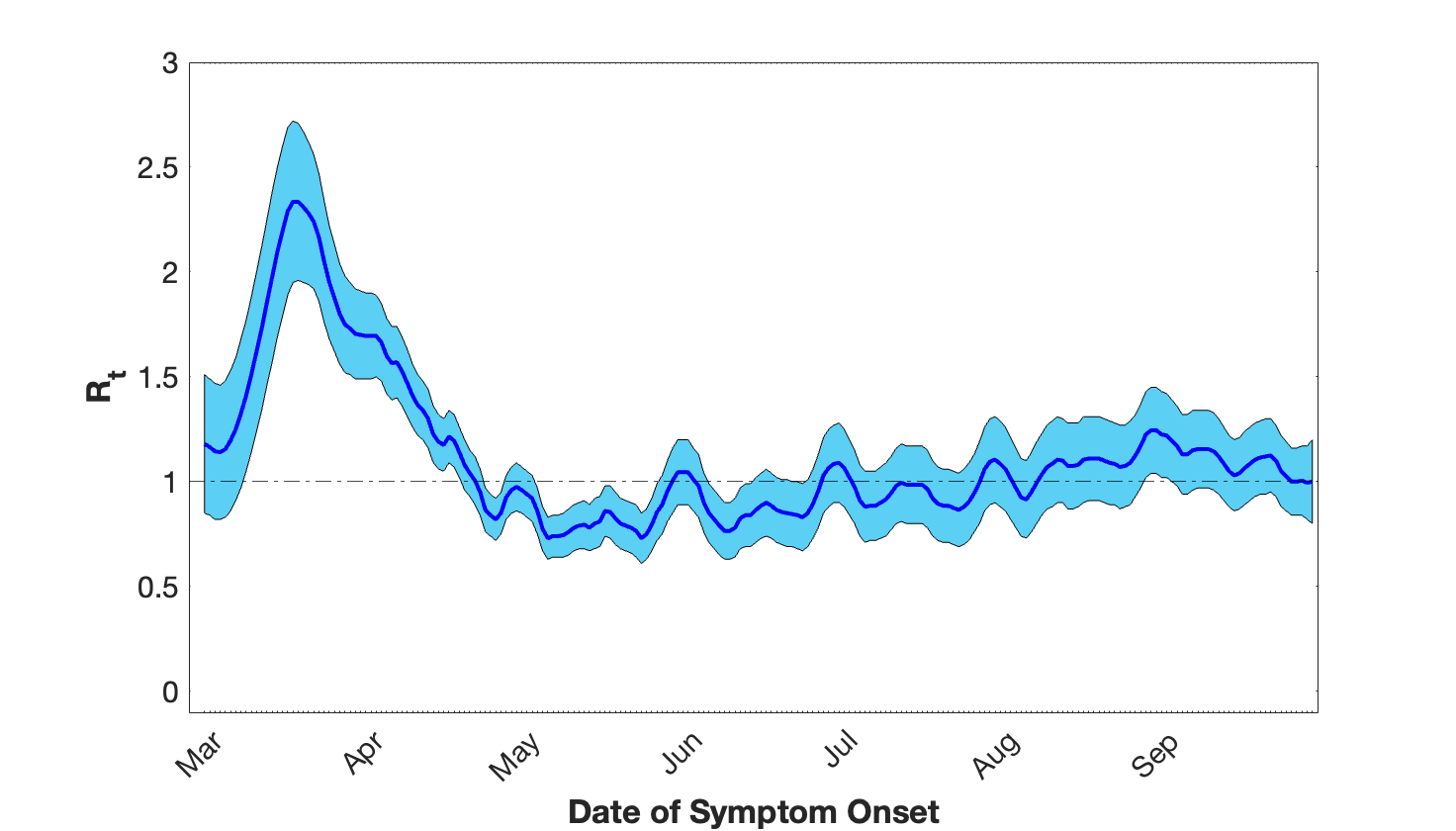
Figure A1: Effective reproduction number ($R_{t}$) in Manaus, Brazil in 2020 as a function of Date of Symptom Onset. Light blue indicates $95\%$ confidence interval around dark blue mean. Figure adapted from Figure S7.D in Buss et al., “Three-quarters attack rate of SARS-CoV-2 in the Brazilian Amazon during a largely unmitigated epidemic” ([4]).

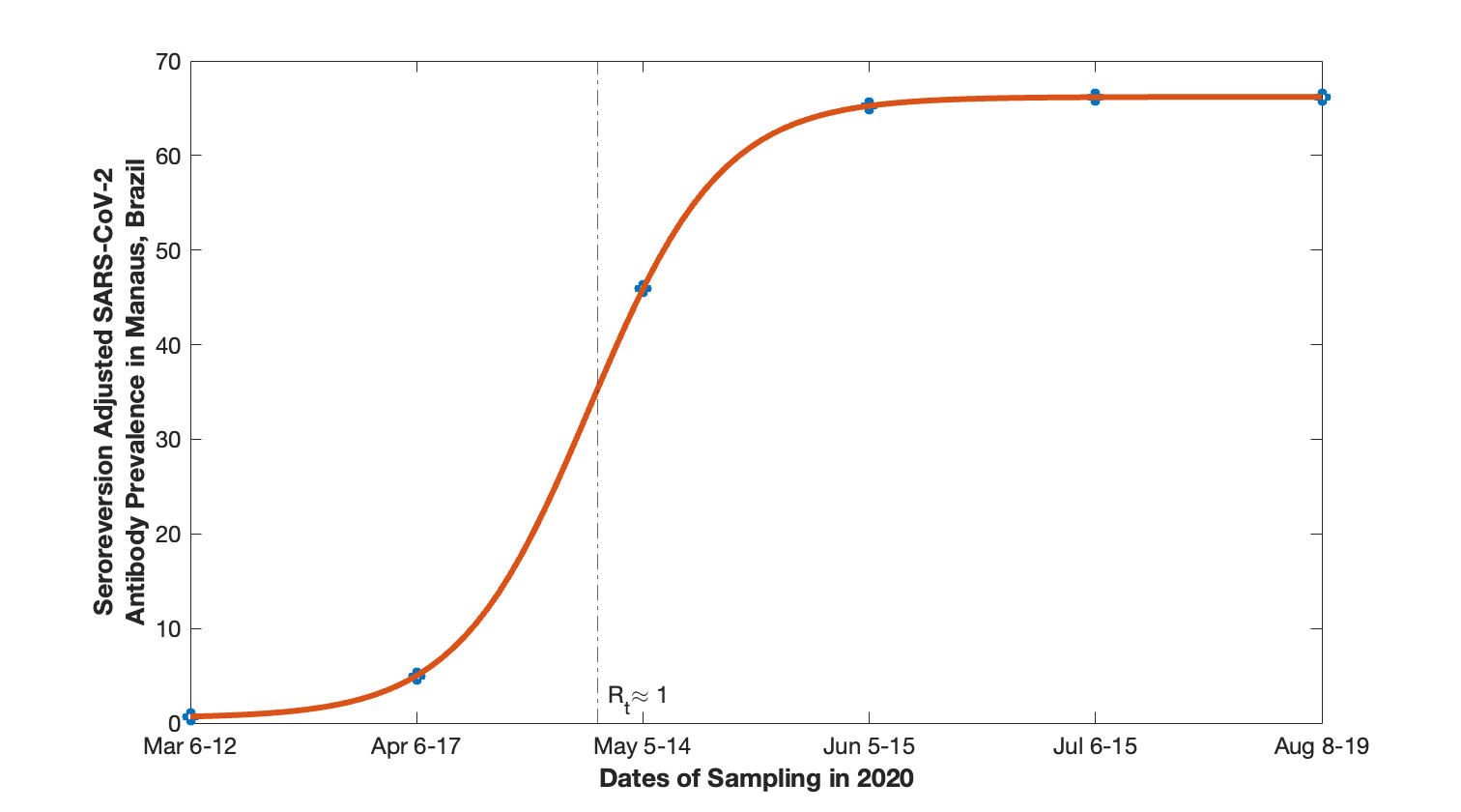
Figure A2: Mean cumulative antibody prevalence in Manaus, Brazil in 2020. Seroreversion adjustment done with a 1.4 S/C threshold. Figure adapted from the red points in Figure 2A and Table S2 in Buss et al., “Three-quarters attack rate of SARS-CoV-2 in the Brazilian Amazon during a largely unmitigated epidemic” ([4]).

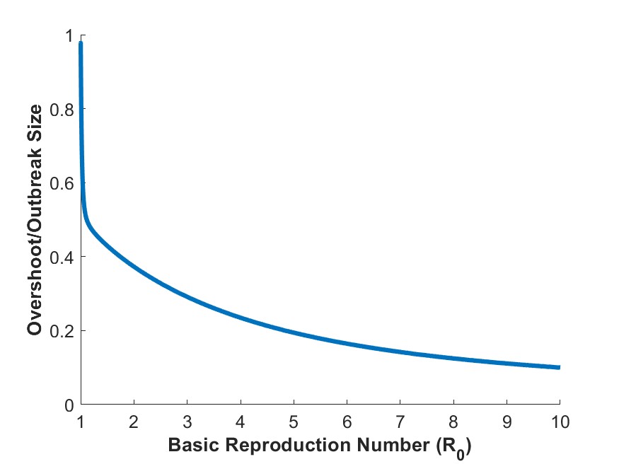
Figure A3: The ratio of individuals infected in the overshoot phase compared to total outbreak size as a function of $R_{0}$.

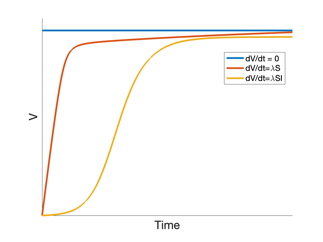
Figure A4: The fraction of population that is vaccinated (V) based on different vaccination rates: a vaccination rate of zero over the course of the epidemic (blue), a constant per-capita vaccination rate (red), and a risk-driven vaccination rate (yellow).

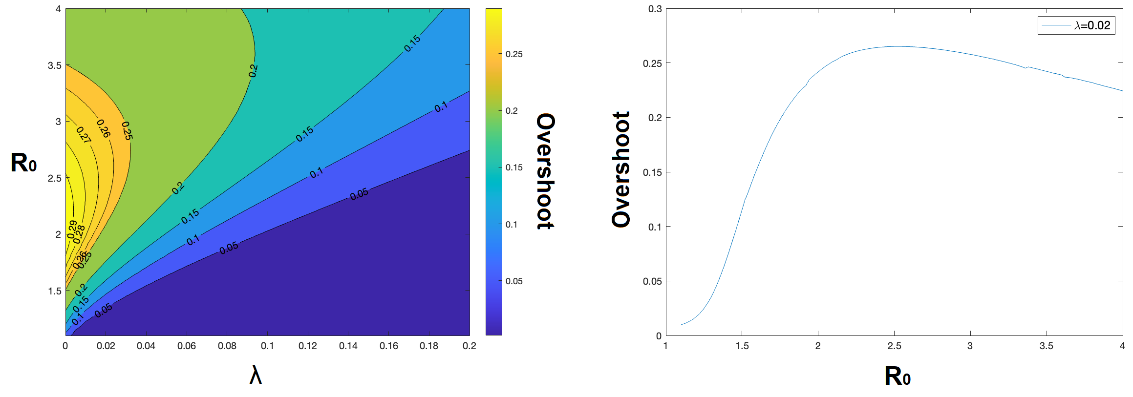
Figure A5: a) Contour plot for the overshoot for the SIRV model with $\frac{dV}{dt}=\lambda S$ as a function of $\lambda$ and $R_{0}$. b) Vertical cross-section of the contour plot from (a) for $\lambda=0.02$.

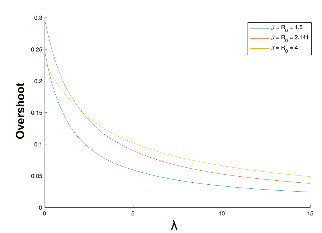
Figure A6: The overshoot for the SIRV model with $\frac{dV}{dt}=\lambda SI$ as a function of $\lambda$ for different levels of $\beta$ (or equivalently $R_{0}$).

Code to Generate Figures

Code executed in MATLAB R2022b

⬇

1%%%%%%%%%%%%%%%%%%%%%%%%%%%%%%%%%%%%%%%%%%%%%%%

2% Figure 1

3tspan = 0:0.001:50;

4I0_frac = 0.001;

5vFrac = 0;

6R_final = zeros(length(vFrac),1);

7OvershootCalc = zeros(length(20),1);

8for x = 1:length(vFrac)

9 v_frac = vFrac(x);

10 SIR_0 = [1-I0_frac-v_frac; I0_frac; 0; vFrac];

11 for y = 1%:20

12 beta = 1.5;%.*(1-vFrac); %y; %2.15128 ./ (1-v_frac);

13 gamma = 1;

14 [t,SIR] = ode45(@(t,SIR) SIR_dynamics(t,SIR,beta,gamma,v_frac), tspan, SIR_0);

15 HIT_time = find(SIR(:,2) == max(SIR(:,2)));

16 S_star = SIR(HIT_time,1);

17 S_inf = SIR(length(SIR),1);

18 R_final(x,1) = SIR(length(SIR),3);

19 OvershootCalc(y,1) = S_star - S_inf;

20 end

21 disp(x)

22end

23

24%%%%%%%%%%%%% Plot 1a: Overshoot in terms of S

25close all

26figure

27subplot(1,2,1)

28hold on

29plot(t(:,1),SIR(:,1),’b-’);

30plot(t(:,1),SIR(:,2),’r-’);

31plot(t(:,1),SIR(:,3),’g-’);

32ylim([0 1])

33set(gca,’XTick’,[])

34%% Plot special lines

35xl = xline(t(HIT_time),’-.’,{’t^*’},’FontSize’, 15);

36xl.LabelVerticalAlignment = ’top’;

37xl.LabelOrientation = ’horizontal’;

38yline(S_star,’-.’,{’S(t^*)’},’FontSize’, 15)

39yline(S_inf,’-.’,{’S(t=\infty)’},’FontSize’, 15)

40%% Labels

41xlabel(’Time’,’FontSize’, 30,’FontWeight’,’bold’)

42set(gca,’TickLabelInterpreter’, ’tex’,’FontSize’, 15)

43ylabel(’Fraction of Population’,’FontSize’, 30,’FontWeight’,’bold’)

44set(gca,’TickLabelInterpreter’, ’tex’,’FontSize’, 15)

45legend(’S’,’I’,’R’,’FontSize’, 15)%,’R’)

46

47%%%%%%%%%%%%%%%%% Plot 1b: Overshoot in terms of incidence

48%figure

49subplot(1,2,2)

50hold on

51set(gca,’XTick’,[])

52set(gca,’TickLabelInterpreter’, ’tex’,’FontSize’, 15)

53yyaxis left

54ylabel(’Fraction of Population’,’FontSize’, 30,’FontWeight’,’bold’)

55set(gca,’TickLabelInterpreter’, ’tex’,’FontSize’, 15)

56plot(t(:,1),SIR(:,1),’b-’);

57plot(t(:,1),SIR(:,2),’r-’);

58plot(t(:,1),beta.*SIR(:,1).*SIR(:,2),’r-.’);

59ylim([0 1])

60%% Plot special lines

61xl = xline(t(HIT_time),’-.’,{’t^*’},’FontSize’, 15);

62xl.LabelVerticalAlignment = ’top’;

63xl.LabelOrientation = ’horizontal’;

64shaded = area(t(HIT_time:end,1), beta.*SIR(HIT_time:end,1).*SIR(HIT_time:end,2), ’FaceColor’, [1, 1, 0]);

65%% Labels

66xlabel(’Time’,’FontSize’, 20,’FontWeight’,’bold’)

67legend(’S’,’I’,’\betaSI’,’FontSize’, 15)%,’R’)

68yyaxis right

69ylabel(’\betaSI’, ’FontSize’,20,’FontWeight’,’bold’)

70

71

72

73%%%%%%%%%%%%%%%%%%%%%%%%%%%%%%%%%%%%%%%%%%%%%%%

74% Figure 2

75%%%%%%%%%%%%%%%%%%%%%%%%%%%%%%%%%%%%%%%%%%%%%%%%%%

76%%%%%%%%%%%%%%%%%% Overshoot as function of R_0

77

78tspan = 0:0.001:50;

79I0_frac = 0.001;

80SIR_0 = [1-I0_frac; I0_frac; 0; I0_frac];

81beta_range = 1.05:0.01:10;

82gamma_range = [1];

83vFrac = 0;

84

85overshoot_vec = zeros(length(beta_range),length(gamma_range));

86R_0_vec = zeros(length(beta_range),length(gamma_range));

87overshoot2FAR = zeros(length(beta_range),length(gamma_range));

88FAR = zeros(length(beta_range),length(gamma_range));

89for y = 1:length(gamma_range)

90 for x = 1:length(beta_range)

91 [t,SIR] = ode45(@(t,SIR) SIR_dynamics(t,SIR,beta_range(1,x),gamma_range(1,y),vFrac), tspan, SIR_0);

92

93 HIT_time = find(SIR(:,2) == max(SIR(:,2)));

94 S_star = SIR(HIT_time,1);

95 S_inf = SIR(length(SIR),1);

96 overshoot_vec(x,y) = S_star - S_inf;

97 R_0_vec(x,y) = beta_range(1,x) ./ gamma_range(1,y);

98 overshoot2FAR(x,y) = (S_star - S_inf)./(1-S_inf);

99 FAR(x,y) = 1-S_inf;

100 end

101end

102

103figure

104plot(R_0_vec(:,y),overshoot_vec(:,y),’-’)

105ylim([0 0.35])

106hold on

107max_over = find(overshoot_vec(:,y) == max(overshoot_vec(:,y)));

108xl = xline(R_0_vec(max_over),’r-.’,{’R_0^*’},’FontSize’, 12);

109xl.LabelVerticalAlignment = ’bottom’;

110xl.LabelOrientation = ’horizontal’;

111yl = yline(max(overshoot_vec(:,y)),’r-.’,{’Overshoot^*’},’FontSize’, 12);

112xlabel(’R_0’,’FontSize’, 15)

113ylabel(’Overshoot’,’FontSize’, 15)

114

115

116%%%%%%%%%%%%%%%%%%%%%%%%%%%%%%%%%%%%%%%%%%%%%%%

117% Figure A1

118

119% Data given by Direct Correspondence with authors of Buss et. al, Science 2020, “Three-quarters attack rate of SARS-CoV-2 in the Brazilian Amazon during a largely unmitigated epidemic”.

120

121% This figure is an adaptation of S7.D in their Supplementary Material

122

123% Raw data compiled from Rt_Science_buss -> symptoms_csv -> tdates_MN_symp.csv & Rlow_MN_symp.csv & Rhigh_MN_symp.csv into following Table.

124

125

126

127Time Point Lower Bound on 95% CI for Rt Upper Bound on 95% CI for Rt Date

1281 1.35 3.08 2/3/20

1292 1.38 3.02 2/4/20

1303 1.39 2.92 2/5/20

1314 1.37 2.8 2/6/20

1325 1.34 2.67 2/7/20

1336 1.3 2.54 2/8/20

1347 1.26 2.42 2/9/20

1358 1.21 2.3 2/10/20

1369 1.18 2.2 2/11/20

13710 1.15 2.12 2/12/20

13811 1.12 2.05 2/13/20

13912 1.1 1.99 2/14/20

14013 1.07 1.93 2/15/20

14114 1.05 1.89 2/16/20

14215 1.03 1.84 2/17/20

14316 1.01 1.8 2/18/20

14417 0.98 1.75 2/19/20

14518 0.96 1.72 2/20/20

14619 0.95 1.68 2/21/20

14720 0.93 1.65 2/22/20

14821 0.92 1.63 2/23/20

14922 0.91 1.62 2/24/20

15023 0.91 1.6 2/25/20

15124 0.9 1.59 2/26/20

15225 0.89 1.57 2/27/20

15326 0.88 1.55 2/28/20

15427 0.87 1.53 2/29/20

15528 0.85 1.51 3/1/20

15629 0.84 1.49 3/2/20

15730 0.82 1.47 3/3/20

15831 0.82 1.46 3/4/20

15932 0.83 1.48 3/5/20

16033 0.86 1.53 3/6/20

16134 0.91 1.59 3/7/20

16235 0.97 1.68 3/8/20

16336 1.05 1.77 3/9/20

16437 1.14 1.88 3/10/20

16538 1.24 2 3/11/20

16639 1.34 2.12 3/12/20

16740 1.46 2.25 3/13/20

16841 1.57 2.38 3/14/20

16942 1.69 2.5 3/15/20

17043 1.79 2.6 3/16/20

17144 1.89 2.69 3/17/20

17245 1.95 2.72 3/18/20

17346 1.96 2.71 3/19/20

17447 1.95 2.67 3/20/20

17548 1.94 2.62 3/21/20

17649 1.92 2.56 3/22/20

17750 1.86 2.47 3/23/20

17851 1.76 2.34 3/24/20

17952 1.68 2.22 3/25/20

18053 1.62 2.13 3/26/20

18154 1.56 2.04 3/27/20

18255 1.52 1.98 3/28/20

18356 1.51 1.95 3/29/20

18457 1.49 1.92 3/30/20

18558 1.49 1.91 3/31/20

18659 1.49 1.9 4/1/20

18760 1.49 1.9 4/2/20

18861 1.5 1.89 4/3/20

18962 1.48 1.85 4/4/20

19063 1.42 1.78 4/5/20

19164 1.39 1.74 4/6/20

19265 1.4 1.74 4/7/20

19366 1.36 1.69 4/8/20

19467 1.31 1.63 4/9/20

19568 1.26 1.56 4/10/20

19669 1.22 1.51 4/11/20

19770 1.2 1.48 4/12/20

19871 1.16 1.44 4/13/20

19972 1.09 1.36 4/14/20

20073 1.06 1.32 4/15/20

20174 1.05 1.3 4/16/20

20275 1.09 1.34 4/17/20

20376 1.07 1.32 4/18/20

20477 1.02 1.26 4/19/20

20578 0.96 1.2 4/20/20

20679 0.93 1.15 4/21/20

20780 0.89 1.12 4/22/20

20881 0.84 1.06 4/23/20

20982 0.76 0.97 4/24/20

21083 0.74 0.94 4/25/20

21184 0.72 0.92 4/26/20

21285 0.75 0.95 4/27/20

21386 0.82 1.03 4/28/20

21487 0.85 1.07 4/29/20

21588 0.86 1.09 4/30/20

21689 0.85 1.07 5/1/20

21790 0.83 1.05 5/2/20

21891 0.81 1.03 5/3/20

21992 0.75 0.97 5/4/20

22093 0.67 0.88 5/5/20

22194 0.63 0.83 5/6/20

22295 0.64 0.84 5/7/20

22396 0.64 0.84 5/8/20

22497 0.64 0.85 5/9/20

22598 0.65 0.87 5/10/20

22699 0.67 0.89 5/11/20

227100 0.68 0.9 5/12/20

228101 0.68 0.91 5/13/20

229102 0.67 0.89 5/14/20

230103 0.68 0.92 5/15/20

231104 0.69 0.93 5/16/20

232105 0.74 0.98 5/17/20

233106 0.73 0.98 5/18/20

234107 0.7 0.95 5/19/20

235108 0.68 0.92 5/20/20

236109 0.67 0.91 5/21/20

237110 0.66 0.9 5/22/20

238111 0.64 0.89 5/23/20

239112 0.61 0.85 5/24/20

240113 0.63 0.87 5/25/20

241114 0.67 0.92 5/26/20

242115 0.72 0.99 5/27/20

243116 0.75 1.03 5/28/20

244117 0.81 1.1 5/29/20

245118 0.85 1.16 5/30/20

246119 0.89 1.2 5/31/20

247120 0.89 1.2 6/1/20

248121 0.89 1.2 6/2/20

249122 0.86 1.16 6/3/20

250123 0.83 1.13 6/4/20

251124 0.76 1.04 6/5/20

252125 0.71 0.99 6/6/20

253126 0.68 0.96 6/7/20

254127 0.65 0.93 6/8/20

255128 0.63 0.9 6/9/20

256129 0.63 0.9 6/10/20

257130 0.64 0.92 6/11/20

258131 0.68 0.97 6/12/20

259132 0.69 0.99 6/13/20

260133 0.69 0.99 6/14/20

261134 0.71 1.02 6/15/20

262135 0.73 1.04 6/16/20

263136 0.74 1.06 6/17/20

264137 0.73 1.04 6/18/20

265138 0.71 1.02 6/19/20

266139 0.7 1.01 6/20/20

267140 0.69 1.01 6/21/20

268141 0.69 1 6/22/20

269142 0.68 1 6/23/20

270143 0.67 0.99 6/24/20

271144 0.69 1.01 6/25/20

272145 0.73 1.06 6/26/20

273146 0.78 1.13 6/27/20

274147 0.85 1.21 6/28/20

275148 0.88 1.25 6/29/20

276149 0.9 1.27 6/30/20

277150 0.9 1.28 7/1/20

278151 0.88 1.25 7/2/20

279152 0.84 1.2 7/3/20

280153 0.8 1.15 7/4/20

281154 0.74 1.08 7/5/20

282155 0.71 1.05 7/6/20

283156 0.72 1.05 7/7/20

284157 0.72 1.05 7/8/20

285158 0.73 1.07 7/9/20

286159 0.74 1.09 7/10/20

287160 0.77 1.12 7/11/20

288161 0.8 1.16 7/12/20

289162 0.81 1.18 7/13/20

290163 0.8 1.17 7/14/20

291164 0.8 1.17 7/15/20

292165 0.8 1.17 7/16/20

293166 0.8 1.17 7/17/20

294167 0.78 1.15 7/18/20

295168 0.74 1.1 7/19/20

296169 0.72 1.07 7/20/20

297170 0.71 1.06 7/21/20

298171 0.71 1.06 7/22/20

299172 0.7 1.05 7/23/20

300173 0.69 1.04 7/24/20

301174 0.7 1.06 7/25/20

302175 0.72 1.09 7/26/20

303176 0.76 1.13 7/27/20

304177 0.8 1.19 7/28/20

305178 0.86 1.26 7/29/20

306179 0.89 1.3 7/30/20

307180 0.9 1.31 7/31/20

308181 0.88 1.29 8/1/20

309182 0.86 1.26 8/2/20

310183 0.82 1.21 8/3/20

311184 0.78 1.16 8/4/20

312185 0.74 1.11 8/5/20

313186 0.73 1.1 8/6/20

314187 0.76 1.14 8/7/20

315188 0.8 1.19 8/8/20

316189 0.84 1.23 8/9/20

317190 0.87 1.27 8/10/20

318191 0.88 1.29 8/11/20

319192 0.9 1.31 8/12/20

320193 0.9 1.3 8/13/20

321194 0.87 1.28 8/14/20

322195 0.87 1.28 8/15/20

323196 0.88 1.28 8/16/20

324197 0.9 1.31 8/17/20

325198 0.91 1.31 8/18/20

326199 0.91 1.31 8/19/20

327200 0.91 1.31 8/20/20

328201 0.9 1.3 8/21/20

329202 0.89 1.29 8/22/20

330203 0.89 1.28 8/23/20

331204 0.87 1.27 8/24/20

332205 0.88 1.27 8/25/20

333206 0.89 1.29 8/26/20

334207 0.93 1.32 8/27/20

335208 0.97 1.37 8/28/20

336209 1.02 1.43 8/29/20

337210 1.04 1.45 8/30/20

338211 1.04 1.45 8/31/20

339212 1.02 1.43 9/1/20

340213 1.02 1.42 9/2/20

341214 1 1.39 9/3/20

342215 0.98 1.36 9/4/20

343216 0.94 1.32 9/5/20

344217 0.94 1.32 9/6/20

345218 0.96 1.34 9/7/20

346219 0.97 1.34 9/8/20

347220 0.97 1.34 9/9/20

348221 0.97 1.34 9/10/20

349222 0.96 1.33 9/11/20

350223 0.94 1.3 9/12/20

351224 0.91 1.26 9/13/20

352225 0.88 1.22 9/14/20

353226 0.86 1.2 9/15/20

354227 0.87 1.21 9/16/20

355228 0.89 1.24 9/17/20

356229 0.91 1.26 9/18/20

357230 0.93 1.28 9/19/20

358231 0.94 1.29 9/20/20

359232 0.94 1.3 9/21/20

360233 0.95 1.3 9/22/20

361234 0.93 1.27 9/23/20

362235 0.88 1.22 9/24/20

363236 0.86 1.19 9/25/20

364237 0.84 1.16 9/26/20

365238 0.84 1.16 9/27/20

366239 0.84 1.17 9/28/20

367240 0.82 1.17 9/29/20

368241 0.8 1.2 9/30/20

369

370

371

372close all

373Buss_RtManaus = table2array(WaveTable(:,1:3))’; %Import table above as “WaveTable”

374

375figure

376x_allData = Buss_RtManaus(1,:);

377y_allData = mean(Buss_RtManaus([2,3],:));

378x = x_allData(1,28:end); %Only plot starting from March 1 (which is data point 28 out of the full data set)

379y = y_allData(1,28:end);

380curve1 = Buss_RtManaus(2,28:end);

381curve2 = Buss_RtManaus(3,28:end);

382x2 = [x, fliplr(x)];

383inBetween = [curve1, fliplr(curve2)];

384fill(x2, inBetween, [0.3569,0.8118,0.9569]);

385hold on;

386plot(x, y, ’b’, ’LineWidth’, 2);

387xticks(28:27+length(x))

388xticklabels(table2cell(RlowMNsymp(28:end,4)));

389xtickangle(45)

390xlabel(’Date of Symptom Onset’,’FontSize’, 24, ’FontWeight’,’bold’)

391set(gca,’TickLabelInterpreter’, ’tex’,’FontSize’, 15)

392ylabel(’R_t’,’FontSize’, 24, ’FontWeight’,’bold’)

393set(gca,’TickLabelInterpreter’, ’tex’,’FontSize’, 15)

394ylim([-0.1, 3])

395xlim([25, 242])

396ax = gca;

397ax.TickLength = [0.001,0.001];

398yline(1,’k-.’,’FontSize’,12)

399

400

401

402

403%%%%%%%%%%%%%%%%%%%%%%%%%%%%%%%%%%%%%%%%%%%%%%%

404% Figure A2

405%%%%%%%%%%%%

406

407%% Data taken from table S2 in Supplemental Information of Buss et. al, Science 2020, “Three-quarters attack rate of SARS-CoV-2 in the Brazilian Amazon during a largely unmitigated epidemic”.

408

409

410Prevalence_seroreversionAdj = [0.7, 5, 45.9, 65.2, 66.2, 66.2];%, 72.2, 76];

411Prevalence_seroreversionAdj_lowerbound = [0.2, 3.7, 41.8, 60.5, 61.5, 61.8, 64.3, 66.6];

412Prevalence_seroreversionAdj_upperbound = [1.5, 6.6, 50.6, 74.3, 80.1, 80.9, 91.8, 97.9];

413Prevalence_dates = {’Mar 6-12’, ’Apr 6-17’, ’May 5-14’, ’Jun 5-15’, ’Jul 6-15’, ’Aug 8-19’}; %, ’Sep 5-14’, ’Oct 10-17’};

414% Define the logistic function to fit

415logisticFun = @(params, x) params(1) + (params(2) - params(1)) ./ (1 + exp(-params(3) .* (x - params(4))));

416% Initial guess for the parameters [a, b, c, d] of the logistic function

417initialGuess = [0, 1, 1, 5];

418% Fit the logistic function using lsqcurvefit

419fitParams = lsqcurvefit(logisticFun, initialGuess, 1:length(Prevalence_seroreversionAdj), Prevalence_seroreversionAdj);

420% Generate a finer grid of x values for plotting the fitted curve

421xFit = linspace(min(1:length(Prevalence_seroreversionAdj)), max(1:length(Prevalence_seroreversionAdj)), 100);

422% Calculate the corresponding y values for the fitted curve

423yFit = logisticFun(fitParams, xFit);

424% Plot the original data points and the fitted curve

425figure;

426p = plot(1:length(Prevalence_seroreversionAdj), Prevalence_seroreversionAdj, ’o’, xFit, yFit, ’-’, ’LineWidth’,3);

427xlabel(’Dates of Sampling in 2020’,’FontSize’,12,’FontWeight’,’bold’)

428xticks(1:length(Prevalence_dates))

429ylabel([’Seroreversion Adjusted SARS-CoV-2’, newline, ’Antibody Prevalence in Manaus, Brazil’],’FontSize’,12,’FontWeight’,’bold’)

430%title(’Manaus COVID-19 First Wave’)

431xticklabels(Prevalence_dates);

432set(gca,’TickLabelInterpreter’, ’tex’,’FontSize’, 12)

433hold on

434yl = xline(2.8,’-.’,’R_t\approx 1’,’FontSize’, 12);

435yl.LabelVerticalAlignment = ’bottom’;

436yl.LabelOrientation = ’horizontal’;

437

438

439%%%%%%%%%%%%%%%%%%%%%%%%%%%%%%%%%%%%%%%%%%%%%%%

440% Figure A3

441

442close all

443% Epidemic Overshoot as a Function of R0 in MATLAB

444% Varying R0 values

445R0_values = [1:0.001:1.12,1.13:0.01:10];

446% Initialize overshoot values

447overshoot_values = zeros(size(R0_values));

448overshoot_fracvalues = zeros(size(R0_values));

449for i = 1:length(R0_values)

450 % Parameters

451 R0 = R0_values(i);

452 beta = R0 * gamma;

453 % Solve the ODE system

454 odeSystem = @(t, y) [-beta * y(1) * y(2); % dS/dt

455 beta * y(1) * y(2) - gamma * y(2); % dI/dt

456 gamma * y(2)]; % dR/dt

457 [~, y] = ode89(odeSystem, tspan, initialConditions);

458 % Find the peak of infections and its corresponding time index

459 [maxInfections, peakIndex] = max(y(:, 2));

460 % Calculate the epidemic overshoot (difference in fraction of susceptible)

461 overshoot = y(peakIndex, 1) - y(end, 1);

462 overshoot_values(i) = overshoot;

463 overshoot_fracvalues(i) = overshoot ./ (1-y(end, 1));

464end

465

466figure

467xlabel(’Basic Reproduction Number (R_0)’, ’FontSize’,14, ’FontWeight’,’bold’);

468ylabel(’Overshoot/Outbreak Size’,’FontSize’,14, ’FontWeight’,’bold’);

469hold on

470p = plot(R0_values, overshoot_fracvalues, ’-.’, ’LineWidth’,3);

471set(gca,’FontSize’,12)

472

473

474%%%%%%%%%%%%%%%%%%%%%%%%%%%%%%%%%%%%%%%%%%%%%%%

475% Figure A4

476

477%% Save SIR_dynamics2 as a separate file.

478% function dSIR = SIR_dynamics2(t,SIR,beta,gamma,lambda)

479% dSIR = zeros(4,1);

480% dSIR(1) = -beta*SIR(1)*SIR(2) - lambda*SIR(1);

481% dSIR(2) = beta*SIR(1)*SIR(2) - gamma*SIR(2);

482% dSIR(3) = gamma*SIR(2);

483% dSIR(4) = lambda*SIR(1);

484%%

485

486tspan = 0:0.001:20;

487I0_frac = 0.001;

488vFrac = 0;

489gamma = 1;

490beta = 2;

491lambda = 0.0;

492SIR_0 = [1-I0_frac-vFrac; I0_frac; 0; vFrac]

493[t,SIR] = ode45(@(t,SIR) SIR_dynamics2(t,SIR,beta,gamma,lambda), tspan, SIR_0);

494figure

495hold on

496plot(t,SIR(:,4)+0.075,’LineWidth’,3)

497xlabel(’Time’, ’FontSize’, 20)

498ylabel(’V’, ’FontSize’, 20)

499set(gca,’XTick’,[]);

500set(gca,’YTick’,[]);

501lambda = 0.04;

502beta = 5;

503[t,SIR] = ode45(@(t,SIR) SIR_dynamics2(t,SIR,beta,gamma,lambda), tspan, SIR_0);

504hold on

505plot(t,SIR(:,4),’LineWidth’,3)

506lambda = 0.2;

507beta = 2;

508[t,SIR] = ode45(@(t,SIR) SIR_dynamics3(t,SIR,beta,gamma,lambda), tspan, SIR_0);

509hold on

510plot(t,SIR(:,4),’LineWidth’,3)

511legend( ’dV/dt = 0’, ’dV/dt=\lambdaS’,’dV/dt=\lambdaSI’,’FontSize’,14)

512

513

514%%%%%%%%%%%%%%%%%%%%%%%%%%%%%%%%%%%%%%%%%%%%%%%

515% Figure A5

516

517%close all

518tspan = 0:0.01:100;

519I0_frac = 0.001;

520lambda = [0:0.001:0.2]’;

521betas = [1.1:0.001:4]’;

522R_final = zeros(length(lambda),length(betas));

523OvershootCalc = zeros(length(lambda),length(betas));

524VacFrac = zeros(length(lambda),length(betas));

525

526for x = 1:length(lambda)

527 lambdaVal = lambda(x);

528 SIR_0 = [1-I0_frac; I0_frac; 0; 0];

529 for y = 1:length(betas)

530 beta = betas(y); % ./ (1-v_frac);

531 gamma = 1;

532 [t,SIR] = ode45(@(t,SIR) SIR_dynamics2(t,SIR,beta,gamma,lambdaVal), tspan, SIR_0);

533 HIT_time = find(SIR(:,2) == max(SIR(:,2)));

534 S_star = SIR(HIT_time,1);

535 S_inf = SIR(length(SIR),1);

536 R_final(x,y) = SIR(length(SIR),3);

537 OvershootCalc(x,y) = (SIR(HIT_time,1)+SIR(HIT_time,4)) - (SIR(length(SIR),1)+SIR(length(SIR),4));

538 VacFrac(x,y) = SIR(length(SIR),4);

539 eps_time = find(SIR(:,2) == 0.001);

540 end

541end

542

543%% FIGURE FOR lambda S model

544figure

545subplot(1,2,1)

546[Xs,Ys]=meshgrid(lambda,betas);

547%[Xs,Ys]=meshgrid(lambda(1:31),betas);

548contourf(Xs’,Ys’,OvershootCalc,[0,0.05,0.1,0.15,0.2,0.25:0.01:0.3],"ShowText",true)

549%contourf(Xs’,Ys’,OvershootCalc(1:31,:),"ShowText",true)

550xlabel(’\lambda’,’FontSize’,20,’FontWeight’,’bold’)

551ylabel(’R_0’,’FontSize’, 20, ’FontWeight’, ’bold’)

552set(gca,’FontSize’, 15)

553%title(’Overshoot’)

554c = colorbar;

555c.Label.String = ’Overshoot’;

556%% Cross-section of Contour Plot

557subplot(1,2,2)

558plot(betas./gamma,OvershootCalc(5,:))

559xlabel(’R_0’, ’FontSize’, 16, ’FontWeight’, ’bold’)

560ylabel(’Overshoot’, ’FontSize’, 16, ’FontWeight’, ’bold’)

561legend(’\lambda=0.02’,’FontSize’,12)

562

563

564

565

566%%%%%%%%%%%%%%%%%%%%%%%%%%%%%%%%%%%%%%%%%%%%%%%

567% Figure A6

568

569

570%%%%%%%%%%%%%%%%%% Overshoot as function of Lambda in dV/dt=lambdaSI vaccine model

571tspan = 0:0.001:50;

572I0_frac = 0.001;

573SIR_0 = [1-I0_frac; I0_frac; 0; 0];

574beta_range = [1.5, 2.141, 4];

575gamma = 1;

576lambda_range = [0:0.1:15];

577

578overshoot_vec = zeros(length(beta_range),length(lambda_range));

579

580for x = 1:length(beta_range)

581 for y = 1:length(lambda_range)

582 [t,SIR] = ode78(@(t,SIR) SIR_dynamics3(t,SIR,beta_range(x), gamma, lambda_range(y)), tspan, SIR_0);

583

584 HIT_time = find(SIR(:,2) == max(SIR(:,2)));

585 S_star = SIR(HIT_time,1)+SIR(HIT_time,4); %Recall overshoot in a vaccine model requires consideration of Susceptibles and vaccinated individuals (eqn A23)

586 S_inf = SIR(length(SIR),1)+SIR(length(SIR),4);

587 overshoot_vec(x,y) = S_star - S_inf;

588 end

589end

590

591figure

592hold on

593plot(1:length(SIR),SIR(:,1))

594plot(1:length(SIR),SIR(:,2))

595plot(1:length(SIR),SIR(:,3))

596plot(1:length(SIR),SIR(:,4))

597

598figure

599hold on

600plot(lambda_range,overshoot_vec(1,:),’-’)

601plot(lambda_range,overshoot_vec(2,:),’-’)

602plot(lambda_range,overshoot_vec(3,:),’-’)

603xlabel(’\lambda’,’FontSize’, 15)

604ylabel(’Overshoot’,’FontSize’, 15)

605legend(’\beta=R_0=1.5’, ’\beta=R_0=2.141’, ’\beta=R_0=4’)

References

- [1] Andreas Handel, Ira M Longini and Rustom Antia “What is the best control strategy for multiple infectious disease outbreaks?” Publisher: Royal Society In Proceedings of the Royal Society B: Biological Sciences 274.1611, 2007, pp. 833–837 DOI: 10.1098/rspb.2006.0015
- [2] Sarah Cobey “Modeling infectious disease dynamics” Publisher: American Association for the Advancement of Science In Science 368.6492, 2020, pp. 713–714 DOI: 10.1126/science.abb5659
- [3] William Ogilvy Kermack, A.. McKendrick and Gilbert Thomas Walker “A contribution to the mathematical theory of epidemics” Publisher: Royal Society In Proceedings of the Royal Society of London. Series A, Containing Papers of a Mathematical and Physical Character 115.772, 1927, pp. 700–721 DOI: 10.1098/rspa.1927.0118
- [4] Lewis F. Buss et al. “Three-quarters attack rate of SARS-CoV-2 in the Brazilian Amazon during a largely unmitigated epidemic” Publisher: American Association for the Advancement of Science In Science 371.6526, 2021, pp. 288–292 DOI: 10.1126/science.abe9728
- [5] Fred Brauer “The Kermack–McKendrick epidemic model revisited” In Mathematical Biosciences 198.2, 2005, pp. 119–131 DOI: 10.1016/j.mbs.2005.07.006
- [6] D. Breda et al. “On the formulation of epidemic models (an appraisal of Kermack and McKendrick)” Publisher: Taylor & Francis _eprint: https://doi.org/10.1080/17513758.2012.716454 In Journal of Biological Dynamics 6, 2012, pp. 103–117 DOI: 10.1080/17513758.2012.716454
- [7] Md Arif Billah, Md Mamun Miah and Md Nuruzzaman Khan “Reproductive number of coronavirus: A systematic review and meta-analysis based on global level evidence” Publisher: Public Library of Science In PLOS ONE 15.11, 2020, pp. e0242128 DOI: 10.1371/journal.pone.0242128
- [8] World Health Organization “Consensus document on the epidemiology of severe acute respiratory syndrome (SARS)” number-of-pages: 46, 2003 URL: https://apps.who.int/iris/handle/10665/70863
- [9] Shaun A Truelove et al. “Clinical and Epidemiological Aspects of Diphtheria: A Systematic Review and Pooled Analysis” In Clinical Infectious Diseases 71.1, 2020, pp. 89–97 DOI: 10.1093/cid/ciz808
- [10] Rebecca Grant, Liem-Binh Luong Nguyen and Romulus Breban “Modelling human-to-human transmission of monkeypox” In Bulletin of the World Health Organization 98.9, 2020, pp. 638–640 DOI: 10.2471/BLT.19.242347
- [11] Z… Wong, C.. Bui, A.. Chughtai and C.. Macintyre “A systematic review of early modelling studies of Ebola virus disease in West Africa” Publisher: Cambridge University Press In Epidemiology & Infection 145.6, 2017, pp. 1069–1094 DOI: 10.1017/S0950268817000164
- [12] Veronika I. Zarnitsyna et al. “Intermediate levels of vaccination coverage may minimize seasonal influenza outbreaks” Publisher: Public Library of Science In PLOS ONE 13.6, 2018, pp. e0199674 DOI: 10.1371/journal.pone.0199674
- [13] Robert M. May “Vaccination programmes and herd immunity” Number: 5892 Publisher: Nature Publishing Group In Nature 300.5892, 1982, pp. 481–483 DOI: 10.1038/300481a0
- [14] Julien Arino et al. “A final size relation for epidemic models” Publisher: American Institute of Mathematical Sciences In Mathematical Biosciences & Engineering 4.2, 2007, pp. 159
- [15] Fred Brauer “Age-of-infection and the final size relation” Publisher: American Institute of Mathematical Sciences In Mathematical Biosciences & Engineering 5.4, 2008, pp. 681
- [16] Horst R. Thieme “Mathematics in Population Biology” Google-Books-ID: 9f9aDwAAQBAJ Princeton University Press, 2018
- [17] Odo Diekmann, Hans Heesterbeek and Tom Britton “Mathematical Tools for Understanding Infectious Disease Dynamics” Princeton University Press, 2013
- [18] Mario Castro, Saúl Ares, José A. Cuesta and Susanna Manrubia “The turning point and end of an expanding epidemic cannot be precisely forecast” Publisher: Proceedings of the National Academy of Sciences In Proceedings of the National Academy of Sciences 117.42, 2020, pp. 26190–26196 DOI: 10.1073/pnas.2007868117