Upper Bounds on Overshoot in SIR Models with Nonlinear Incidence

Abstract

We expand the calculation of the upper bound on epidemic overshoot in SIR models to account for nonlinear incidence. We lay out the general procedure and restrictions to perform the calculation analytically. We show why the infected fraction must enter linearly into the incidence term, whereas the susceptible fraction can enter more generically, including non-monotonically. We demonstrate the procedure by working through several examples. We also numerically study what happens to the upper bound on overshoot when nonlinear incidence manifests in the form of dynamics over a contact network.

Introduction

Compartmental models have been an invaluable tool for analyzing the dynamics of epidemics for the last century. The SIR ordinary differential equation (ODE) variation of the model is one of the most popular due to its relative simplicity and has received a lot of attention in both the academic literature and the public health arena [1, 2]. The most basic form of the SIR model, known as the Kermack-McKendrick ODE model, assumes a bilinear incidence rate $\beta SI$ for the growth term of the infected compartment, with transmissibility parameter $\beta$ and first-order (i.e. linear) with respect to the fraction of population that is susceptible ($S$) and infected ($I$).

A significant body of work in the literature has been done to generalize this incidence term into more complicated forms [3, 4, 5, 6, 7, 8]. Moving beyond bilinear forms towards nonlinear incidence allows for the consideration of models with more biological complexity and realism. Factors such as network effects, seasonality, and non-pharmaceutical interventions are known to give rise to more complex dynamics [9, 10, 11, 12].

The overshoot is a feature of the SIR model that has recently received more attention [13, 14, 15, 16]. The overshoot quantifies the number of individuals that become infected after the prevalence peak of infections occur. In more colloquial terms, it gives the damage caused by the epidemic after the peak. An upper bound on the overshoot in the SIR model was first numerically observed by [17]. More recent work has illustrated a general mathematical path to analytically calculate the upper bound on epidemic overshoot [18]. Here we lay the foundation to calculate the upper bound for overshoot when considering incidence terms beyond the simple bilinear case.

The equations of the Kermack-McKendrick SIR ODE model are given as follows with generic incidence term $\beta f(S)g(I)$, where $f(S)$ and $g(I)$ are functions of $S$ and $I$ respectively to be specified.

$$\frac{dS}{dt} =-\beta f(S)g(I)$$ (1)

$$\frac{dI}{dt} =\beta f(S)g(I)-\gamma I$$ (2)

$$\frac{dR}{dt} =\gamma I$$ (3)

where $S$, $I$, $R\in[0,1]$ are the fractions of the population that are susceptible, infected, and recovered respectively, $\beta,\gamma\in\mathbb{R}_{>0}$ are positive-definite parameters for transmission and recovery rate respectively.

For the SIR model, the overshoot is given by the following equation:

$$Overshoot=S_{t^{*}}-S_{\infty}$$ (4)

where $S_{t^{*}}$ is the fraction of susceptibles at the time of the prevalence peak (i.e. when $I$ is maximal in value), $t^{*}$, and $S_{\infty}$ is the fraction of susceptibles at the end of the epidemic. To solve this equation, the easiest approach is to derive an equation for $S_{t^{*}}$ in terms of only $S_{\infty}$ and parameters. We do this by first setting (2) equal to 0 and solving for the critical susceptible fraction $S_{t^{*}}$.

$$\frac{dI}{dt} =0=\beta f(S_{t^{*}})g(I_{t^{*}})-\gamma I_{t^{*}}$$

By using the usual definition for the basic reproduction number, $R_{0}\equiv\frac{\beta}{\gamma}$, we obtain the following equation for $S_{t^{*}}$.

$$S_{t^{*}} =f^{-1}(\frac{I_{t^{*}}}{g(I_{t^{*}})}\frac{1}{R_{0}})$$

We can see from this equation that $S_{t^{*}}$ will have $I$ dependence unless $g(I_{t^{*}})=I_{t^{*}}$. Thus to make what follows analytically tractable, let us assume $g(I_{t^{*}})=I_{t^{*}}$. We will provide even stronger justification why $g(I)$ must take this form later in the results. This assumption of $g(I_{t^{*}})=I_{t^{*}}$ reduces the above equation to the following.

$$S_{t^{*}} =f^{-1}(\frac{1}{R_{0}})$$ (6)

Taking this equation for $S_{t^{*}}$ (6) and the overshoot formula (4), we obtain:

$$Overshoot=f^{-1}(\frac{1}{R_{0}})-S_{\infty}$$ (7)

Thus the main challenge now becomes a problem of finding an equation for $R_{0}$ and the inverse function $f^{-1}$. Based on the results originally derived by Nguyen et. al. [18], the following outlines the general steps for calculating the maximal overshoot for a SIR model:

1. Take the ratio of $\frac{dI}{dt}$ and $\frac{dS}{dt}$. Integrate the resulting ratio. Ideally, the integration yields a conserved quantity.

2. Evaluate the equation for the conserved quantity at the beginning of the epidemic ($t=0$) and the end of the epidemic ($t=\infty$) using initial conditions and asymptotic values. Then, rearrange the resulting equation for $\frac{1}{R_{0}}$.

3. Find the form for the inverse function, $f^{-1}$.

4. Combine the equations for $\frac{1}{R_{0}}$ and $f^{-1}$ with the overshoot equation.

5. Maximize the resulting overshoot equation by taking the derivative of the equation with respect to $S_{\infty}$ and setting the equation to 0 to find the extremal point $S_{\infty}^{*}$. This step usually leads to a transcendental equation for $S_{\infty}^{*}$, which can be solved numerically.

6. Use the maximizing $S_{\infty}^{*}$ value in the overshoot equation to calculate the corresponding maximal overshoot.

7. Calculate the corresponding $R_{0}^{*}$ using $S_{\infty}^{*}$ and the $\frac{1}{R_{0}}$ equation.

Thus, the analytical exploration of nonlinear incidence terms of the type $\beta f(S)g(I)$ is reduced to exploring different forms of $f(S)$.

Results

Restrictions on $g(I)$

The first step is to rule out what forms for the incidence term will not work with the procedure outlined above.

We now show the principle reason why we require $g(I)=I$. We can see from calculating Step A. in (8) that any incidence term that does not take the form $g(I)=aI,a\in\mathbb{R}$, where $a$ is a real scalar, retains $I$ dependence upon simplification.

$$\text{Step \ref{step1}: }\frac{\frac{dI}{dt}}{\frac{dS}{dt}}=\frac{\beta f(S)g(I)-\gamma I}{-\beta f(S)g(I)}=-1+\frac{I}{R_{0}f(S)g(I)}$$ (8)

Any deviation from the form $g(I)=aI$ results in $I$ in the numerator and the denominator not completely cancelling out which will result in having to integrate $I$ with respect to $S$, which we will not be able to do analytically. Therefore, $I$ must enter linearly into the incidence term. Since $a$ can be absorbed into the $\beta$ parameter, all possible incidence terms for the purpose of calculating overshoot analytically will take the form $\beta\cdot f(S)\cdot I$.

Restrictions on $f(S)$

We now turn to what restrictions there are on the form of $f(S)$. We start first with the two boundary conditions for $S$. First, we must enforce that:

$$f(S=0)=0$$ (9)

Otherwise, since $I$ does not have such a restriction, violating this condition leaves open the possibility of having $\frac{dS}{dt}$ (1) be non-zero when the number of susceptibles is zero, which is not realistic.

For the second boundary condition, we must have that:

$$f(S=1)>\frac{\gamma}{\beta}=\frac{1}{R_{0}}$$ (10)

This is obtained by inspecting $\frac{dI}{dt}$ (2) and ensuring that the incidence term $\beta f(S)g(I)$ is larger than the recovery term $\gamma I$ at $t=0$. Otherwise, the epidemic never starts. Assuming $I_{0}$ is sufficiently small, then $S$ is approximately $1$ at $t=0$.

Beyond the boundary conditions, an obvious requirement is that $f(S)$ should be a continuous function. In order to be able to calculate the maximal overshoot analytically, the function should be integratable with respect to $S$ and should also have a closed-form inverse $f^{-1}$. As we will demonstrate, non-monotonic functions for $f(S)$ are possible.

For $f(S)$, the following examples are constructed using basic functions that satisfy the above criteria:

1. $exp(S)-1$

2. Invertible polynomials of $S$

3. $sin(aS)$

Conversely, there are many examples of functions that would not work. An example that satisfies the boundary conditions but that does not have a closed form inverse is $f(S)=log(S+1)$. While similar to examples listed, the following violate the boundary conditions: $exp(S),log(S)$, $cos(S)$. Examples that violate conditions of continuity include step functions of $S$ or $f(S)$ with cusps.

Deriving Maximal Overshoot for Various $f(S)$

We now take these examples of allowable $f(S)$ and apply the whole procedure previously outlined for finding the maximal overshoot.

Example 1: $f(S)=exp(S)-1$

First we will consider the exponential form. This produces an incidence term that grows slightly faster than the original bilinear incidence term, and so might be relevant in situations where there are network effects. We start at Step A. by solving for the rate of change of $I$ as a function of $S$ by taking the ratio of $\frac{dI}{dt}$ and $\frac{dS}{dt}$.

$$\frac{dI}{dS} =-1+\frac{1}{R_{0}(e^{S}-1)}$$ (11)

from which it follows on integration using the substitution $u=e^{S}$ that $I+S+\frac{S-ln|e^{S}-1|}{R_{0}}$ is constant along all trajectories.

For Step B., consider the conserved quantity at both the beginning ($t=0$) and end ($t=\infty$) of the epidemic.

$$I_{0}+S_{0}+\frac{S_{0}-ln|e^{S_{0}}-1|}{R_{0}} =I_{\infty}+S_{\infty}+\frac{S_{\infty}-ln|e^{S_{\infty}}-1|}{R_{0}}$$

hence

$$\frac{1}{R_{0}}=\frac{I_{\infty}+S_{\infty}-I_{0}-S_{0}}{S_{0}-S_{\infty}+ln(\frac{|e^{S_{\infty}}-1|}{||e^{S_{0}}-1|})}$$ (12)

We use the initial conditions: $S_{0}=1-\epsilon$ and $I_{0}=\epsilon$, where $\epsilon$ is the (infinitesimally small) fraction of initially infected individuals. We use the standard asymptotic of the SIR model that there are no infected individuals at the end of an SIR epidemic: $I_{\infty}=0$. This yields:

$$\frac{1}{R_{0}} =\frac{S_{\infty}-1}{1-S_{\infty}+ln(\frac{|e^{S_{\infty}}-1|}{e-1})}$$ (13)

For Step C., we find the inverse of $f$.

$$f(x)=e^{S}-1\implies f^{-1}(x)=ln(x+1)$$ (14)

For Step D., we substitute the expression for $\frac{1}{R_{0}}$ (13) and $f^{-1}$ (14) into the overshoot equation (7).

$$Overshoot =ln(\frac{ln(\frac{|e^{S_{\infty}}-1|}{e-1})}{1-S_{\infty}+ln(\frac{|e^{S_{\infty}}-1|}{e-1})})-S_{\infty}$$ (15)

For Step E., differentiation of both sides with respect to $S_{\infty}$ and setting the equation to zero to solve for the critical $S_{\infty}^{*}$ yields:

$$0 =(\frac{ln(\frac{|e^{S^{*}_{\infty}}-1|}{e-1})}{1-S^{*}_{\infty}+ln(\frac{|e^{S^{*}_{\infty}}-1|}{e-1})})^{-1}(\frac{(1-S^{*}_{\infty}+ln(\frac{|e^{S^{*}_{\infty}}-1|}{e-1}))\cdot((\frac{|e^{S^{*}_{\infty}}-1|}{e-1})^{-1}\frac{e^{S^{*}_{\infty}}}{e-1})-(ln(\frac{|e^{S^{*}_{\infty}}-1|}{e-1}))\cdot(-1+(\frac{|e^{S^{*}_{\infty}}-1|}{e-1})^{-1}\frac{e^{S^{*}_{\infty}}}{e-1})}{(1-S^{*}_{\infty}+ln(\frac{|e^{S^{*}_{\infty}}-1|}{e-1}))^{2}})-1$$

Since $e^{S}-1$ is positive semi-definite over the unit interval for $S$, dropping the absolute value symbols and simplifying yields:

$$ln(\frac{e^{S^{*}_{\infty}}-1}{e-1})(ln(\frac{e^{S^{*}_{\infty}}-1}{e-1})-S^{*}_{\infty}) =(1-S^{*}_{\infty})(\frac{e^{S^{*}_{\infty}}}{e^{S^{*}_{\infty}}-1})$$

which admits both a trivial solution ($S_{\infty}^{*}=1$) and the solution $S_{\infty}^{*}=0.1663...$ .

For Step F., using the non-trivial solution for $S_{\infty}^{*}$ in the overshoot equation (15) to obtain the value of the maximal overshoot for this model, $Overshoot^{*}|_{\begin{subarray}{c}{}_{\beta(e^{S}-1)I}\end{subarray}}$ yields:

$$Overshoot^{*}|_{\begin{subarray}{c}{}_{\beta(e^{S}-1)I}\end{subarray}} =0.2963...$$ (17)

Thus, the maximal overshoot for incidence functions of the form $\beta(e^{S}-1)I$ is $0.296...$ .

For Step G., we can calculate the corresponding $R_{0}^{*}$ using $S_{\infty}^{*}$ and (13).

$$R_{0}^{*}|_{\begin{subarray}{c}{}_{\beta(e^{S}-1)I}\end{subarray}} =1.7$$ (18)

This result is verified numerically in Figure 1.

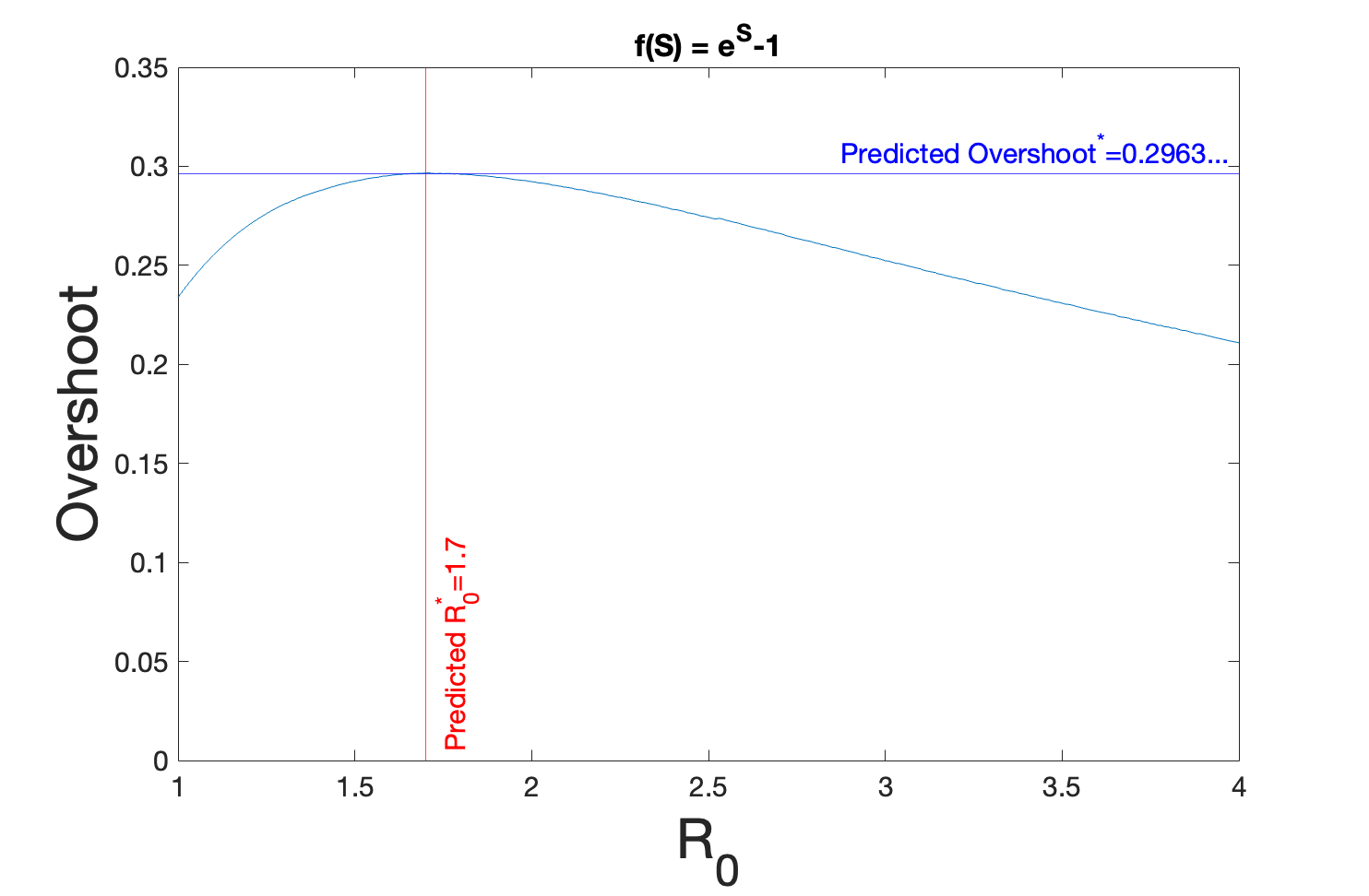
Figure 1: The overshoot as a function of $R_{0}$ for an SIR model with nonlinear incidence term of $\beta(e^{S}-1)I$. The horizontal line for $Overshoot^{*}$ in dark blue and the vertical line in red given by $R_{0}^{*}=1.7$ are the theoretical predictions given by the calculations in the text. The curve is obtained from numerical simulations.

Example 2: $f(S)$ = Invertible Polynomials of $S$

Next, let us consider invertible polynomials. Having access to large degree polynomials will allow us to make arbitrarily sharp incidence terms. While the set of invertible polynomials is a relatively small subset of all polynomials, it still contains an infinitely large number of possible functions. Because the procedure will require integration of $f(S)$ while it is in the denominator, the algebraic details of doing this for higher-order polynomials with lower-order terms can quickly become cumbersome. So let us illustrate a test case using just the leading term of a generic cubic function. Let $f(S)=aS^{3}$, where $a\in\mathbb{R}$.

We start at Step A. by solving for the rate of change of $I$ as a function of $S$ by taking the ratio of $\frac{dI}{dt}$ and $\frac{dS}{dt}$.

$$\frac{dI}{dS} =-1+\frac{1}{R_{0}aS^{3}}$$ (19)

from which it follows on integration that $I+S+\frac{1}{2R_{0}aS^{2}}$ is constant along any trajectory.

For Step B., consider the conserved quantity at both the beginning ($t=0$) and end ($t=\infty$) of the epidemic.

$$I_{0}+S_{0}+\frac{1}{2R_{0}aS_{0}^{2}} =I_{\infty}+S_{\infty}+\frac{1}{2R_{0}aS_{\infty}^{2}}$$

hence

$$\frac{1}{R_{0}} =(I_{\infty}+S_{\infty}-I_{0}-S_{0})\frac{2a(S_{0}S_{\infty})^{2}}{S_{\infty}^{2}-S_{0}^{2}}$$ (20)

Using the initial conditions ($S_{0}=1-\epsilon$ and $I_{0}=\epsilon$, where $\epsilon<<1$) and asymptotic condition ($I_{\infty}=0$) yields:

$$\frac{1}{R_{0}} =\frac{2aS_{\infty}^{2}}{S_{\infty}+1}$$ (21)

For Step C., we find the inverse of $f$.

$$f(x)=ax^{3}\implies f^{-1}(x)=(\frac{x}{a})^{1/3}$$ (22)

For Step D., we substitute the expression for $\frac{1}{R_{0}}$ (21) and $f^{-1}$ (22) into the overshoot equation (7).

$$Overshoot =(\frac{2S_{\infty}^{2}}{S_{\infty}+1})^{1/3}-S_{\infty}$$ (23)

For Step E., differentiation with respect to $S_{\infty}$ and setting the equation to zero to solve for the critical $S_{\infty}^{*}$ yields:

$$0 =\frac{1}{3}(\frac{2S_{\infty}^{*2}}{S_{\infty}^{*}+1})^{-2/3}(\frac{(S_{\infty}^{*}+1)\cdot 4S_{\infty}^{*}-2S_{\infty}^{*2}\cdot 1}{(S_{\infty}^{*}+1)^{2}})-1$$ (24)

whose solution is $S_{\infty}^{*}=0.310...$ .

For Step F., using $S_{\infty}^{*}$ in the overshoot equation (23) to obtain the value of the maximal overshoot for this model, $Overshoot^{*}|_{\begin{subarray}{c}{}_{\beta(aS^{3})I}\end{subarray}}$ yields:

$$Overshoot^{*}|_{\begin{subarray}{c}{}_{\beta(aS^{3})I}\end{subarray}} =0.217...$$ (25)

Thus, the maximal overshoot for incidence functions of the form $\beta(aS^{3})I$ is 0.217… .

For Step G., we can calculate the corresponding $R_{0}^{*}$ using $S_{\infty}^{*}$ and (21).

$$R_{0}^{*}|_{\begin{subarray}{c}{}_{\beta(aS^{3})I}\end{subarray}}=\frac{6.816...}{a}$$ (26)

This prediction of the maximal overshoot being independent of $a$, whereas the corresponding critical $R_{0}$ is inversely proportional to $a$ is verified numerical in Figure 2.

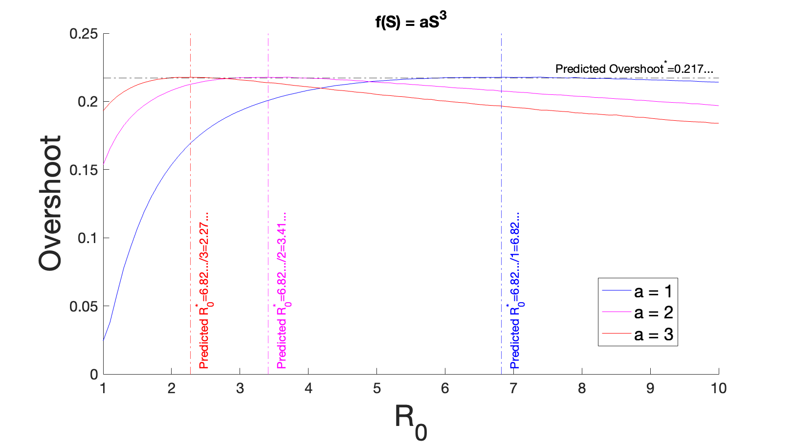
Figure 2: The overshoot as a function of $R_{0}$ for an SIR model with nonlinear incidence term of $\beta(aS^{3})I$ for different values of $a$. The dashed horizontal line for $Overshoot^{*}$ and the dashed vertical lines given by $R_{0}^{*}=1/a$ are the theoretical predictions given by the calculations in the text. The solid curves are obtained from numerical simulations using the value of the $a$ parameter.

Example 3: $f(S)=sin(aS),a>0$

We start at Step A. by solving for the rate of change of $I$ as a function of $S$ by taking the ratio of $\frac{dI}{dt}$ and $\frac{dS}{dt}$.

$$\frac{dI}{dS} =-1+\frac{1}{R_{0}sin(aS)}$$

from which it follows on integration using the substitution $u=csc(aS)+cot(aS)$ that $I+S+\frac{ln|csc(aS)+cot(aS)|}{R_{0}a}$ is constant along all trajectories.

For Step B., consider the conserved quantity at both the beginning ($t=0$) and end ($t=\infty$) of the epidemic.

$$I_{0}+S_{0}+\frac{ln|csc(aS_{0})+cot(aS_{0})|}{R_{0}a} =I_{\infty}+S_{\infty}+\frac{ln|csc(aS_{\infty})+cot(aS_{\infty})|}{R_{0}a}$$

hence

$$\frac{1}{R_{0}}=(I_{\infty}+S_{\infty}-I_{0}-S_{0})\frac{a}{ln\frac{|csc(aS_{0})+cot(aS_{0})|}{|csc(aS_{\infty})+cot(aS_{\infty})|}}$$ (27)

Using the initial conditions ($S_{0}=1-\epsilon$ and $I_{0}=\epsilon$, where $\epsilon<<1$) and asymptotic condition ($I_{\infty}=0$) yields:

$$\frac{1}{R_{0}} =\frac{a(S_{\infty}-1)}{ln(\frac{|csc(a)+cot(a)|}{|csc(aS_{\infty})+cot(aS_{\infty})|})}$$ (28)

For Step C., we find the inverse of $f$.

$$f(x)=sin(ax)\implies f^{-1}(x)=\frac{arcsin(x)}{a}$$ (29)

For Step D., substituting the expression for $\frac{1}{R_{0}}$ (28) and $f^{-1}$ (29) into the overshoot equation (7) yields:

$$Overshoot =\frac{1}{a}arcsin(\frac{a(S_{\infty}-1)}{ln(\frac{|csc(a)+cot(a)|}{|csc(aS_{\infty})+cot(aS_{\infty})|})})-S_{\infty}$$ (30)

For Step E., differentiation of both sides with respect to $S_{\infty}$ and setting the equation to zero to solve for the critical $S_{\infty}^{*}$ yields:

$$0 =\frac{1}{a}(\frac{1}{\sqrt{1-(\frac{a(S_{\infty}^{*}-1)}{ln(\frac{|csc(a)+cot(a)|}{|csc(aS_{\infty}^{*})+cot(aS_{\infty}^{*})|})})^{2}}}\frac{ln(\frac{|csc(a)+cot(a)|}{|csc(aS_{\infty}^{*})+cot(aS_{\infty}^{*})|})\cdot a-a(S_{\infty}^{*}-1)\cdot\frac{\frac{-|csc(a)+cot(a)|\cdot(-acot(aS_{\infty}^{*})csc(aS_{\infty}^{*})-acsc^{2}(aS_{\infty}^{*}))}{(|csc(aS_{\infty}^{*})+cot(aS_{\infty}^{*})|)^{2}}}{\frac{|csc(a)+cot(a)|}{|csc(aS_{\infty}^{*})+cot(aS_{\infty}^{*})|}}}{(ln(\frac{|csc(a)+cot(a)|}{|csc(aS_{\infty}^{*})+cot(aS_{\infty}^{*})|}))^{2}})-1$$ (31)

Solving this transcendental equation (31) requires first specifying the value of parameter $a$. For instance, specifying $a=1$ and solving the equation numerically yields $S_{\infty}^{*}=0.1648...$ .

For Step F., we use $S_{\infty}^{*}$ in the overshoot equation (30) to obtain the value of the maximal overshoot for this model, $Overshoot^{*}|_{\begin{subarray}{c}{}_{\beta(sin(aS))I}\end{subarray}}$. For $a=1$, we obtain:

$$Overshoot^{*}|_{\begin{subarray}{c}{}_{\beta(sin(S))I}\end{subarray}} =0.2931...$$ (32)

Thus, the maximal overshoot for incidence functions of the form $\beta(sin(S))I$ is 0.293… .

For Step G., we can calculate the corresponding $R_{0}^{*}$ using $S_{\infty}^{*}$ and (28).

$$R_{0}^{*}|_{\begin{subarray}{c}{}_{\beta(sin(S))I}\end{subarray}} =2.262...$$ (33)

Now consider $a=\frac{2\pi}{3}$, which produces a non-monotonic $f(S)$ over the unit interval (Figure 3a). Solving (31) for $a=\frac{2\pi}{3}$ yields $S_{\infty}^{*}=0.1163...$ . Repeating Steps F. and G. when $a=\frac{2\pi}{3}$ yields:

$$Overshoot^{*}|_{\begin{subarray}{c}{}_{\beta(sin(\frac{2\pi}{3}S))I}\end{subarray}} =0.2529...$$ (34)

$$R_{0}^{*}|_{\begin{subarray}{c}{}_{\beta(sin(\frac{2\pi}{3}S))I}\end{subarray}} =1.432...$$ (35)

This leads to the question of what the applicable domain of $a$ is. The larger the value of $a$, the stronger the non-monotonicity of $f(S)$ is (Figure 3a). We can first eliminate values based on the second boundary condition (10) which requires that $f(S=1)>\frac{1}{R_{0}}$. Clearly that condition is violated if $f(S=1)$ is not positive, since $\frac{1}{R_{0}}$ is always positive because $\beta$ and $\gamma$ are both positive-definite. Since $f(S)=sin(aS)$, then $f(S)$ is negative when $a\in[\pi n,2\pi n],n=\mathbb{N}$. Furthermore, since we have a formula for $\frac{1}{R_{0}}$ using (28), we can set up the inequality explicitly.

$$f(S=1) >\frac{1}{R_{0}}$$

$$sin(a\cdot 1) >\frac{a(S_{\infty}-1)}{ln(\frac{|csc(a)+cot(a)|}{|csc(aS_{\infty})+cot(aS_{\infty})|})}$$

These result for the different cases of $f(S)=sin(aS)$ are shown in Figure 3b.

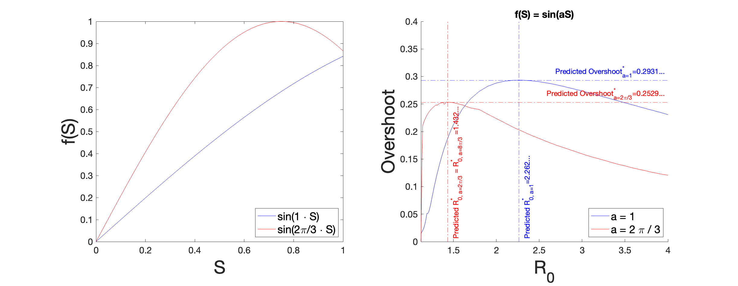
Figure 3: a) $f(S)=sin(aS)$ for different values of $a$. b) The overshoot as a function of $R_{0}$ for an SIR model with nonlinear incidence term of $\beta(sin(aS))I$ for different values of $a$. The dashed horizontal lines for $Overshoot^{*}$ and the dashed vertical lines for $R_{0}^{*}$ are the theoretical predictions given by the calculations in the text. The solid curves are obtained from numerical simulations.

Nonlinear Incidence Generated from Dynamics on Networks

In the previous sections, we focused on nonlinear incidence that was generated from the introduction of a nonlinearity in an ordinary differential equation model. Importantly, this fundamentally assumes homogeneity in the transmission, in that all infected individuals are identical in their ability to spread the disease further. In contrast, network models allow for heterogeneous spreading which depends on the local connectivity of each infected individual. This provides an entirely different mechanism through which nonlinear incidence can be generated compared to the ordinary differential equation models. However, it is difficult to calculate anything analytically for a general network model, so here we do a numerical exploration on the upper bound for overshoot in network models across a range of network structure.

The space of all possible network configurations is immense, so we must restrict ourselves to analyzing a particular subset of possible networks. Here we explore what happens to the overshoot when the contact structure of the population is given by a network graph that is roughly one giant component. While it is possible to construct pathological graphs that produce very complex dynamics, we consider more classical graphs here. Using a parameterization of heterogeneity given by Ozbay et al. [19] (see Methods for details), we simulated epidemics on networks with structure ranging from the homogeneous limit (well-mixed, complete graph) to a heterogeneous limit (heavy-tailed degree distributions). We observed what happens to the overshoot on these different graphs as we changed the transmission probability.

On a network model, where contact structure is made explicit, the homogeneous graph is a complete graph, which recapitulates the well-mixed assumption of the Kermack-McKendrick model. It is not surprising then that the overshoot in the homogeneous graph ($\sigma=0)$ peaks also around 0.3 (Figure 4, $green$), which coincides with the analytical upper bound previously found in the ordinary differential equation Kermack-McKendrick model [18].

We also see that increasing contact heterogeneity qualitatively suppresses the overshoot peak both in terms of the overshoot value and the corresponding transmission probability. Furthermore, increased heterogeneity also flattens out the overshoot curve as a function of transmission probability.

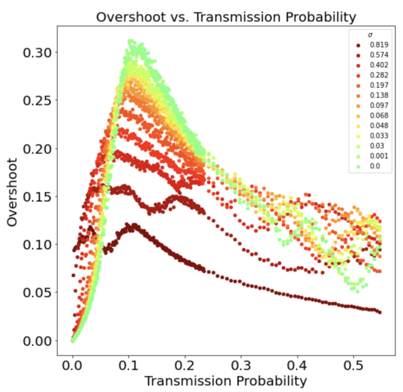
Figure 4: The overshoot for SIR epidemic simulations on networks with varying levels of heterogeneity ($\sigma$) as a function of transmission probability. $N=1000,\lambda=5$. Points represent the average of n = 150 simulation runs.

Discussion

We have illustrated a general method to analytically find the maximal overshoot for generic nonlinear incidence terms. Starting with the general incidence term $\beta f(S)g(I)$, we have deduced what restrictions must be placed on the form of $f(S)$ and $g(I)$ to make an analytical calculation possible. As long as the conditions for a suitable $f(S)$ are satisfied, in principle the maximal overshoot can be derived. However, in the examples shown, we have seen that even relatively simple forms for $f(S)$ can quickly lead to complicated integrals and derivatives. For these examples, we have shown the predictions given by the theoretical calculations generally match the empirical results derived from numerical simulation. The last example of $f(S)=sin(aS)$ is particularly important because it can be used to probe the restrictions on the shape of $f(S)$. The case of $a=\frac{2\pi}{3},f(S)=sin(\frac{2\pi}{3}S)$ demonstrated that $f(S)$ no longer had to be monotonic.

Nonlinear incidence introduced through having a network structure showed that having network connectivity that was more heterogeneous resulted in a reduction in the upper bound on overshoot and a reduction of the dependence of overshoot on transmission overall. Numerically, the overshoot for a homogeneously connected network (i.e. a complete graph) well-approximates a Kermack-McKendrick ODE model. Thus, an upper bound on the overshoot of approximately $0.3$ in both models [18] is perhaps unsurprising.

It will also be interesting to see if more complicated nonlinear interaction terms than the ones presented here can be derived. In addition, it will also be interesting to see how these nonlinear incidence terms interact when additional complexity is added to the SIR model, such as the addition of vaccinations or multiple subpopulations.

Methods

Generating Graphs of Differing Heterogeneity

In Figure 4, we presented the results of SIR simulations of epidemics run on graphs of size N = 1000 and $\lambda=5$, where the parameter of interest is $\sigma$. Each curve, from red to green, represents a different value of the graph heterogeneity. We implemented the following procedure from [19] for generating graphs as a function of a continuous parameter ($\sigma$):

The following simple procedure generates a graph that has the desired heterogeneity:

1. Choose values of $\sigma$ (heterogeneity), $\lambda$ (mean/median node degree), and $N$ (number of nodes).

2. Draw N random samples from the following distribution using $\sigma$ and $\lambda$, rounding these samples to the nearest integer, since the degree of a node can only take on integer values.

   $$f(x;\lambda,\sigma)=\frac{-\ln(\sigma)}{\lambda}(\frac{x}{\lambda})^{-\ln(\sigma)-1}e^{-(x/\lambda)^{(}-\ln(\sigma))};x\geq 0;\sigma\in(0,1];\lambda>\mathbb{R}^{+}$$

3. With the sampled degree distribution from the previous step, now use the configuration model method [20] (which samples over the space of all possible graphs corresponding to a particular degree distribution) to generate a corresponding graph.

This yields a valid graph with the desired amount of heterogeneity as specified by $\sigma$.

Simulating Epidemics on Graphs of Differing Heterogeneity

We implemented the following simulation procedure from [19] for implementing an SIR epidemic on a graph:

Given a graph $G(\sigma)$ of heterogeneity $\sigma$, fix a transmission probability $\tau$ and recovery probability $\gamma$:

1. At time $t_{0}$, fix a small fraction $f$ of nodes to be chosen uniformly on the graph and assign them to the Infected state. The remaining $(1-f)$ fraction of nodes start as Susceptible.

2. For each $i\in[1,T]$, for each pair of adjacent S and I nodes, the susceptible node becomes infected with probability $\tau$.

3. For each $i\in[1,T]$, each infected node recovers with probability $\gamma$.

4. At time $T$, record two quantities: The final attack rate and the herd immunity threshold at the peak of the epidemic.

5. Repeat steps (1-4) n = 150 times for each value of $\tau$.

6. Repeat steps (1-5) for each value of $\sigma$.

Numerical Solutions and Code

Where needed, equations were solved numerically using the $ode45$ numerical solver in $MATLAB$. Code for all sections can be provided upon request.

Author Contributions

M.M.N. designed research, performed research, and wrote and reviewed the manuscript.

References

- [1] Roy M. Anderson and Robert M. May “Infectious Diseases of Humans: Dynamics and Control” OUP Oxford, 1992
- [2] Odo Diekmann, Hans Heesterbeek and Tom Britton “Mathematical Tools for Understanding Infectious Disease Dynamics” Princeton University Press, 2013
- [3] Wei-min Liu, Simon A. Levin and Yoh Iwasa “Influence of nonlinear incidence rates upon the behavior of SIRS epidemiological models” In Journal of Mathematical Biology 23.2, 1986, pp. 187–204 DOI: 10.1007/BF00276956
- [4] Wei-min Liu, Herbert W. Hethcote and Simon A. Levin “Dynamical behavior of epidemiological models with nonlinear incidence rates” In Journal of Mathematical Biology 25.4, 1987, pp. 359–380 DOI: 10.1007/BF00277162
- [5] H.. Hethcote and P. Driessche “Some epidemiological models with nonlinear incidence” In Journal of Mathematical Biology 29.3, 1991, pp. 271–287 DOI: 10.1007/BF00160539
- [6] Shigui Ruan and Wendi Wang “Dynamical behavior of an epidemic model with a nonlinear incidence rate” In Journal of Differential Equations 188.1, 2003, pp. 135–163 DOI: 10.1016/S0022-0396(02)00089-X
- [7] Yu Jin, Wendi Wang and Shiwu Xiao “An SIRS model with a nonlinear incidence rate” In Chaos, Solitons & Fractals 34.5, 2007, pp. 1482–1497 DOI: 10.1016/j.chaos.2006.04.022
- [8] Andrei Korobeinikov “Global Properties of Infectious Disease Models with Nonlinear Incidence” In Bulletin of Mathematical Biology 69.6, 2007, pp. 1871–1886 DOI: 10.1007/s11538-007-9196-y
- [9] Tom Britton, Frank Ball and Pieter Trapman “A mathematical model reveals the influence of population heterogeneity on herd immunity to SARS-CoV-2” Publisher: American Association for the Advancement of Science In Science 369.6505, 2020, pp. 846–849 DOI: 10.1126/science.abc6810
- [10] Alexei V. Tkachenko et al. “Time-dependent heterogeneity leads to transient suppression of the COVID-19 epidemic, not herd immunity” Publisher: Proceedings of the National Academy of Sciences In Proceedings of the National Academy of Sciences 118.17, 2021, pp. e2015972118 DOI: 10.1073/pnas.2015972118
- [11] M. M. Gomes et al. “Individual variation in susceptibility or exposure to SARS-CoV-2 lowers the herd immunity threshold” In Journal of Theoretical Biology 540, 2022, pp. 111063 DOI: 10.1016/j.jtbi.2022.111063
- [12] Antonio Montalbán, Rodrigo M. Corder and M. M. Gomes “Herd immunity under individual variation and reinfection” In Journal of Mathematical Biology 85.1, 2022, pp. 2 DOI: 10.1007/s00285-022-01771-x
- [13] Andreas Handel, Ira M Longini and Rustom Antia “What is the best control strategy for multiple infectious disease outbreaks?” Publisher: Royal Society In Proceedings of the Royal Society B: Biological Sciences 274.1611, 2006, pp. 833–837 DOI: 10.1098/rspb.2006.0015
- [14] Glenn Ellison “Implications of Heterogeneous SIR Models for Analyses of COVID-19”, Working Paper Series 27373 National Bureau of Economic Research, 2020 DOI: 10.3386/w27373
- [15] Łukasz Rachel “An Analytical Model of Covid-19 Lockdowns” In Center for Macroeconomics, 2020
- [16] David I. Ketcheson “Optimal control of an SIR epidemic through finite-time non-pharmaceutical intervention” In Journal of Mathematical Biology 83.1, 2021, pp. 7 DOI: 10.1007/s00285-021-01628-9
- [17] Veronika I. Zarnitsyna et al. “Intermediate levels of vaccination coverage may minimize seasonal influenza outbreaks” Publisher: Public Library of Science In PLOS ONE 13.6, 2018, pp. e0199674 DOI: 10.1371/journal.pone.0199674
- [18] Maximilian M. Nguyen, Ari S. Freedman, Sinan A. Ozbay and Simon A. Levin “Fundamental Bound on Epidemic Overshoot in the SIR Model” In Journal of Royal Society Interface (accepted), 2023 URL: https://www.overleaf.com/project/636acfb3296ff4397a1092b2
- [19] Sinan A. Ozbay and Maximilian M. Nguyen “Parameterizing network graph heterogeneity using a modified Weibull distribution” Number: 1 Publisher: SpringerOpen In Applied Network Science 8.1, 2023, pp. 1–12 DOI: 10.1007/s41109-023-00544-9
- [20] Mark Newman “Networks” Google-Books-ID: YdZjDwAAQBAJ Oxford University Press, 2018