Spontaneous collapse by entanglement suppression

Abstract

We study a recently proposed modified Schrödinger equation having an added nonlinear term, which gives rise to disentanglement. The process of quantum measurement is explored for the case of a pair of coupled spins. We find that the deterministic time evolution generated by the modified Schrödinger equation mimics the process of wavefunction collapse. Added noise gives rise to stochasticity in the measurement process. Conflict with both principles of causality and separability can be avoided by postulating that the nonlinear term is active only during the time when subsystems interact. Moreover, in the absence of entanglement, all predictions of standard quantum mechanics are unaffected by the added nonlinear term.

Introduction - In standard quantum mechanics a measurement is described by a two-step process. The first step is governed by the standard Schrödinger equation. To avoid a possible paradoxical outcome of a description based only on the first step (undefined cat state Schrodinger_807 ), a second step is postulated, in which the state vector collapses. However, it has remained unknown how such a second step can be self-consistently added Penrose_4864 ; Leggett_939 ; Leggett_022001 . This difficulty has became known as the problem of quantum measurement.

In this work we explore an alternative to the collapse postulate, which is based on a modified Schrödinger equation that has an added nonlinear term giving rise to disentanglement Buks_355303 ; Buks_025302 . The proposed equation can be constructed for any physical system whose Hilbert space has finite dimensionality, and it does not violate norm conservation of the time evolution. We explore the dynamics of a system made of two coupled spins, and find that disentanglement gives rise to a process similar to state vector collapse.

Other types of nonlinear extensions of quantum mechanics Geller_2200156 have been previously proposed and studied Weinberg_336 ; Weinberg_61 ; Doebner_397 ; Doebner_3764 ; Gisin_5677 ; Kaplan_055002 ; Munoz_110503 . Most previously proposed extensions give rise to a spontaneous collapse Bassi_471 ; Pearle_857 ; Ghirardi_470 ; Bassi_257 ; Arnquist_080401 . In some cases, however, the proposed nonlinear models are inconsistent with well-established physical principles. Moreover, many predictions of standard quantum mechanics, that have been experimentally verified to very high precision, are significantly altered by some of the proposed nonlinear extensions. Such difficulties are discussed below in the final part of this paper for the case of our proposed modified Schrödinger equation. We find that possible conflicts with the principles of causality and separability, and with many experimentally confirmed predictions of standard quantum mechanics, can be avoided by postulating that disentanglement is active only when subsystems interact.

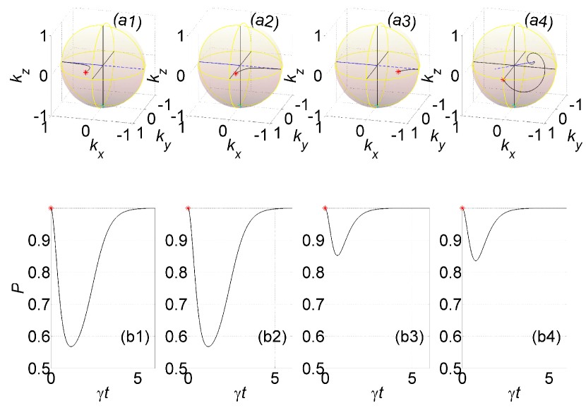
Figure 1: Dipolar measurement. The spin numbers are $S_{1}=1/2$ and $S_{2}=21/2$, the rates are $\gamma=\omega_{\mathrm{d}}=1$, and $\mathbf{\hat{n}}_{2}=-\mathbf{\hat{z}}$ (initial direction of the $S_{2}$ spin, which is labeled by a cyan star symbols). For the plots labeled by the numbers 1, 2 and 3 the dipolar unit vector $\mathbf{\hat{u}}_{\mathrm{d}}$ is given by $\mathbf{\hat{u}}_{\mathrm{d}}=\mathbf{\hat{x}}$ (i.e. $\mathbf{\hat{u}}_{\mathrm{d}}$ is perpendicular to $\mathbf{\hat{n}}_{2}$), whereas $\mathbf{\hat{u}}_{\mathrm{d}}=\left(\sin\left(3\pi/8\right)\cos\left(3\pi/4\right),\sin\left(3\pi/8\right)\sin\left(3\pi/4\right),\cos\left(3\pi/8\right)\right)$ for the plots labeled by the number 4 (i.e. $\mathbf{\hat{n}}_{2}\cdot\mathbf{\hat{u}}_{\mathrm{d}}\neq 0$). At time $t=0$ the spin 1/2 is pointing in the direction $\mathbf{\hat{n}}_{1}=\left(\sin\theta_{1}\cos\varphi_{1},\sin\theta_{1}\sin\varphi_{1},\cos\theta_{1}\right)$, where for (1) $\theta_{1}=0.55\pi$ and $\varphi_{1}=0.45\pi$, for (2) $\theta_{1}=0.55\pi$ and $\varphi_{1}=0.55\pi$, for (3) $\theta_{1}=0.55\pi$ and $\varphi_{1}=0.75\pi$, and for (4) $\theta_{1}=0.5\pi$, and $\varphi_{1}=0.5\pi$. Red star symbols label the initial points $\mathbf{\hat{n}}_{1}$, and the blue solid (dashed) lines connect the origin and the unit vectors $\mathbf{\hat{u}}_{\mathrm{d}}$ ($-\mathbf{\hat{u}}_{\mathrm{d}}$).

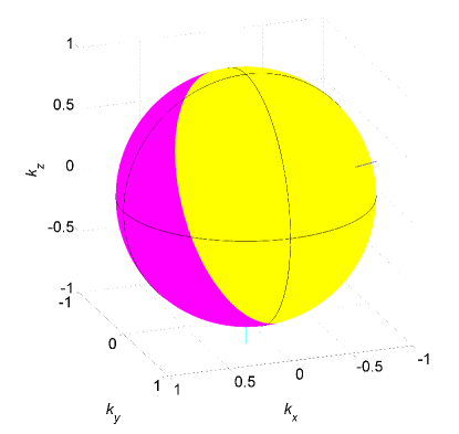
Figure 2: Basins of attraction. All parameters are the same as those used to generate the plots of Fig. 1 labeled by the number 4. Initial direction of the $S_{2}$ spin $\mathbf{\hat{n}}_{2}=-\mathbf{\hat{z}}$ is labeled by a cyan tick, and the dipolar unit vector $\mathbf{\hat{u}}_{\mathrm{d}}=\left(\sin\left(3\pi/8\right)\cos\left(3\pi/4\right),\sin\left(3\pi/8\right)\sin\left(3\pi/4\right),\cos\left(3\pi/8\right)\right)$ is labeled by a blue tick. At time $t=0$ the spin 1/2 is pointing in the direction $\mathbf{\hat{n}}_{1}$. The yellow (purple) colored region is the basin of attraction lying in the hemisphere $\mathbf{\hat{n}}_{1}\cdot\mathbf{\hat{u}}_{\mathrm{d}}>0$ ($\mathbf{\hat{n}}_{1}\cdot\mathbf{\hat{u}}_{\mathrm{d}}<0$), and the corresponding attractor is $\mathbf{\hat{u}}_{\mathrm{d}}$ ($-\mathbf{\hat{u}}_{\mathrm{d}}$).

Disentanglement - Consider a system composed of two subsystems labeled as ’1’ and ’2’, respectively. The dimensionality of the Hilbert spaces of both subsystems, which is denoted by $N_{1}$ and $N_{2}$, respectively, is assumed to be finite. The system is in a normalized pure state vector $\left|\psi\right\rangle$ given by

$$\left|\psi\right\rangle=\mathcal{K}_{1}C\otimes\mathcal{K}_{2}^{\mathrm{T}}\;,$$ (1)

where $C$ is a $N_{1}\times N_{2}$ matrix having entries $C_{k_{1},k_{2}}$, matrix transposition is denoted by $\mathrm{T}$, $\mathcal{K}_{1}=\left(\left|k_{1}\right\rangle_{1},\left|k_{2}\right\rangle_{1},\cdots,\left|k_{N_{1}}\right\rangle_{1}\right)$, $\mathcal{K}_{2}=\left(\left|k_{1}\right\rangle_{2},\left|k_{2}\right\rangle_{2},\cdots,\left|k_{N_{2}}\right\rangle_{2}\right)$, and $\left\{\left|k_{1}\right\rangle_{1}\right\}$ ($\left\{\left|k_{2}\right\rangle_{2}\right\}$) is an orthonormal basis spanning the Hilbert space of subsystem ’1’ (’2’).

The purity $P_{1}$ ($P_{2}$) is defined by $P_{1}=\operatorname{Tr}\rho_{1}^{2}$ ($P_{2}=\operatorname{Tr}\rho_{2}^{2}$), where $\rho_{1}=\operatorname{Tr}_{2}\rho$ ($\rho_{2}=\operatorname{Tr}_{1}\rho$) is the reduced density operator of the first (second) subsystem. By employing the Schmidt decomposition one finds that $P_{1}=P_{2}\equiv P$, where $P=1-\left\langle\mathcal{Q}\right\rangle=1-\left\langle\psi\right|\mathcal{Q}\left|\psi\right\rangle$, the operator $\mathcal{Q}$ is given by [see Eq. (27) of appendix A, and Ref. Buks_QMLN ]

$$\mathcal{Q}=\frac{1}{2}{\displaystyle\sum\limits_{k_{1}^{\prime}<k_{1}^{\prime\prime}}}{\displaystyle\sum\limits_{k_{2}^{\prime}<k_{2}^{\prime\prime}}}\left|\Psi_{k_{1}^{\prime},k_{1}^{\prime\prime},k_{2}^{\prime},k_{2}^{\prime\prime}}\right\rangle\left\langle\Psi_{k_{1}^{\prime},k_{1}^{\prime\prime},k_{2}^{\prime},k_{2}^{\prime\prime}}\right|\;,$$ (2)

and the state $\left\langle\Psi_{k_{1}^{\prime},k_{1}^{\prime\prime},k_{2}^{\prime},k_{2}^{\prime\prime}}\right|$, which depends on the matrix $C$ corresponding to a given state $\left|\psi\right\rangle$, is given by (note that $\left\langle\Psi_{k_{1}^{\prime},k_{1}^{\prime\prime},k_{2}^{\prime},k_{2}^{\prime\prime}}\right|$ is not normalized)

$$\left\langle\Psi_{k_{1}^{\prime},k_{1}^{\prime\prime},k_{2}^{\prime},k_{2}^{\prime\prime}}\right|=C_{{}_{\mathrm{d}}}\left\langle\mathrm{a}\right|+C_{{}_{\mathrm{a}}}\left\langle\mathrm{d}\right|-C_{\mathrm{c}}\left\langle\mathrm{b}\right|-C_{\mathrm{b}}\left\langle\mathrm{c}\right|\;,$$ (3)

where $\mathrm{a}=k_{1}^{\prime},k_{2}^{\prime}$, $\mathrm{b}=k_{1}^{\prime},k_{2}^{\prime\prime}$, $\mathrm{c}=k_{1}^{\prime\prime},k_{2}^{\prime}$ and $\mathrm{d}=k_{1}^{\prime\prime},k_{2}^{\prime\prime}$. Note that $\left\langle\mathcal{Q}\right\rangle=0$ for a product state. In standard quantum mechanics $\left\langle\mathcal{Q}\right\rangle$ is time independent when the subsystems are decoupled (i.e. their mutual interaction vanishes).

As an example, consider a two spin 1/2 system (i.e. $N_{1}=N_{2}=2$) in a pure state $\left|\psi\right\rangle$ given by $\left|\psi\right\rangle=a\left|--\right\rangle+b\left|-+\right\rangle+c\left|+-\right\rangle+d\left|++\right\rangle$. For this case the sum in Eq. (2) contains a single term with $\left\langle\Psi\right|=d\left\langle-,-\right|-c\left\langle-,+\right|-b\left\langle+,-\right|+a\left\langle+,+\right|$, and thus $P=1-2\left|ad-bc\right|^{2}$. Note that for this case $\left\langle\mathcal{Q}\right\rangle\leq 1/2$ (provided that $\left|\psi\right\rangle$ is normalized) Wootters_2245 .

Consider a modified Schrödinger equation for the ket vector $\left|\psi\right\rangle$ having the form

$$\frac{\mathrm{d}}{\mathrm{d}t}\left|\psi\right\rangle=\left[-i\hbar^{-1}\mathcal{H}-\gamma\left(\mathcal{Q}-\left\langle\mathcal{Q}\right\rangle\right)\right]\left|\psi\right\rangle\;,$$ (4)

where $\hbar$ is the Planck’s constant, $\mathcal{H}=\mathcal{H}^{{\dagger}}$ is the Hamiltonian, the rate $\gamma$ is positive, and the operator $\mathcal{Q}$ is given by Eq. (2). The added nonlinear term proportional to $\gamma$ gives rise to disentanglement, however, it has no effect when $\left|\psi\right\rangle$ represents a product state. Note that the norm conservation condition $0=\left(\mathrm{d}/\mathrm{d}t\right)\left\langle\psi\right.\left|\psi\right\rangle$ is satisfied by the modified Schrödinger equation (4).

Dipolar interaction - As an example, the dynamics generated by the modified Schrödinger equation (4) is explored for the case of dipolar interaction between two spins having spin quantum numbers $S_{1}$ and $S_{2}$, respectively. The dipolar interaction is represented by the operator $V_{\mathrm{d}}=\hbar^{-1}\omega_{\mathrm{d}}\left(\mathbf{S}_{1}\cdot\mathbf{\hat{u}}_{\mathrm{d}}\right)\left(\mathbf{S}_{2}\cdot\mathbf{\hat{u}}_{\mathrm{d}}\right)$, where the rate $\omega_{\mathrm{d}}$ is positive, $\mathbf{S}_{n}$ is the spin angular momentum vector operator of the $n$’th spin ($n\in\left\{1,2\right\}$), and $\mathbf{\hat{u}}_{\mathrm{d}}=\left(\sin\theta\cos\varphi,\sin\theta\sin\varphi,\cos\theta\right)$ is a unit vector.

Time evolution examples for the case $S_{1}=1/2$ and $S_{2}=21/2$ are shown by the plots in Fig. 1. The initial state at time $t=0$ is a product state, for which the spin 1/2 is pointing in the direction of the unit vector $\mathbf{\hat{n}}_{1}$ (labeled by a red star symbol), and the spin 21/2 is pointing in the direction of the unit vector $\mathbf{\hat{n}}_{2}=-\mathbf{\hat{z}}$ (labeled by a cyan star symbol). The overlaid blue solid (dashed) lines connect the origin and the dipolar coupling unit vectors $\mathbf{\hat{u}}_{\mathrm{d}}$ ($-\mathbf{\hat{u}}_{\mathrm{d}}$). The spin 1/2 Bloch vector $\mathbf{k}=\left(\hbar/2\right)^{-1}\left\langle\mathbf{S}_{1}\right\rangle$ is numerically calculated by integrating the modified Schrödinger equation (4) for the case $\mathcal{H}=V_{\mathrm{d}}$. The black solid lines in Fig. 1(a1), (a2), (a3) and (a4) represent the spin 1/2 Bloch vector $\mathbf{k}$ evolving from its initial value $\mathbf{\hat{n}}_{1}$ at time $t=0$. The single-spin purity $P=1-\left\langle\mathcal{Q}\right\rangle$ as a function of time $t$ is shown in Fig. 1(b1), (b2), (b3) and (b4).

For the plots in Fig. 1 labeled by the numbers 1, 2 and 3, the dipolar unit vector $\mathbf{\hat{u}}_{\mathrm{d}}$ is given by $\mathbf{\hat{u}}_{\mathrm{d}}=\mathbf{\hat{x}}$ (i.e. $\mathbf{\hat{u}}_{\mathrm{d}}$ is perpendicular to $\mathbf{\hat{n}}_{2}=-\mathbf{\hat{z}}$). These plots, which differ by the initial direction $\mathbf{\hat{n}}_{1}$ of the spin 1/2 (labeled by red star symbols), demonstrate that the Bloch sphere is divided into two basins of attraction. The first (second) basin is the hemisphere $\mathbf{\hat{n}}_{1}\cdot\mathbf{\hat{u}}_{\mathrm{d}}>0$ ($\mathbf{\hat{n}}_{1}\cdot\mathbf{\hat{u}}_{\mathrm{d}}<0$), and the corresponding attractor is $\mathbf{\hat{u}}_{\mathrm{d}}$ ($-\mathbf{\hat{u}}_{\mathrm{d}}$).

While $\mathbf{\hat{n}}_{2}\cdot\mathbf{\hat{u}}_{\mathrm{d}}=0$ for the plots in Fig. 1 labeled by the numbers 1, 2 and 3, the behavior when the initial spin $S_{2}$ direction $\mathbf{\hat{n}}_{2}$ is not perpendicular to the dipolar coupling unit vector $\mathbf{\hat{u}}_{\mathrm{d}}$ is demonstrated by the plots labeled by the number 4. The plot in Fig. 1(a4) shows that the Bloch vector trajectory, from the initial value $\mathbf{\hat{n}}_{1}$ (labeled by the red star symbol) towards the attractor at $\mathbf{\hat{u}}_{\mathrm{d}}$ becomes spiral-like when $\mathbf{\hat{n}}_{2}\cdot\mathbf{\hat{u}}_{\mathrm{d}}\neq 0$. The basins of attraction for this case (i.e. plots in Fig. 1 labeled by the number 4) are shown in Fig. 2. This example demonstrates that the dipolar unit vector $\mathbf{\hat{u}}_{\mathrm{d}}$ determines the spin 1/2 component that is being measured. The measurement process is deterministic however the outcome, which is either $+1$ (when $\mathbf{\hat{n}}_{1}\cdot\mathbf{\hat{u}}_{\mathrm{d}}>0$) or $-1$ (when $\mathbf{\hat{n}}_{1}\cdot\mathbf{\hat{u}}_{\mathrm{d}}<0$) is quantized. This behavior is demonstrated by the green dash-dotted line in Fig. 3, in which the probability $p_{+}$ that the measurement outcome is $+1$ is plotted as a function of the angle $\theta_{1}=\cos^{-1}\left(\mathbf{\hat{n}}_{1}\cdot\mathbf{\hat{u}}_{\mathrm{d}}\right)$. For comparison, the red solid line represents the Born rule of standard quantum mechanics, for which $p_{+}\left(\theta_{1}\right)=\cos^{2}\left(\theta_{1}/2\right)$. A simplified model is employed below to explore noise-induced stochasticity.

Noise - The effect of external noise is taken into account by applying a random rotation to the initial spin 1/2 Block vector $\mathbf{\hat{n}}_{1}$. The random rotation is characterized by an axis normal to $\mathbf{\hat{n}}_{1}$, and by a rotation angle $\phi_{\mathrm{r}}$. As an example, consider the case where the rotation angle $\phi_{\mathrm{r}}$ has a wrapped Cauchy probability distribution $f\left(\phi_{\mathrm{r}}\right)$ given by

$$f\left(\phi_{\mathrm{r}}\right)=\frac{1}{2\pi}\frac{\sinh\phi_{0}}{\cosh\phi_{0}-\cos\phi_{\mathrm{r}}}\;,$$ (5)

where $\phi_{0}>0$ is a scale factor. Consider a rotated frame, in which the dipolar unit vector $\mathbf{\hat{u}}_{\mathrm{d}}$ is parallel to the unit vector $\mathbf{\hat{z}}$. The unit vector $\mathbf{\hat{n}}_{1}$ in this frame is denoted by $\mathbf{\hat{n}}_{1\mathrm{R}}$. The probability $p_{+}$ that the measurement outcome is $+1$ is calculated by spherical integration over the hemisphere $z^{\prime}\geq 0$

$$p_{+}=\frac{1}{4\pi}\int_{0}^{\pi/2}\mathrm{d}\theta^{\prime}\;\sin\theta^{\prime}\int_{0}^{2\pi}\mathrm{d}\varphi^{\prime}\;\frac{4f\left(\theta_{1\mathrm{R}}\right)}{\sin\theta_{1\mathrm{R}}}\;,$$ (6)

where $\theta_{1\mathrm{R}}=\cos^{-1}\left(\mathbf{\hat{n}}_{1\mathrm{R}}\cdot\mathbf{\hat{n}}^{\prime}\right)$, and where $\mathbf{\hat{n}}^{\prime}=\left(\sin\theta^{\prime}\cos\varphi^{\prime},\sin\theta^{\prime}\sin\varphi^{\prime},\cos\theta^{\prime}\right)$. As can be seen from the blue dashed line in Fig. 3, which is calculated using Eq. (6) with a scale factor of $\phi_{0}=0.5$, noise-induced stochasticity mimics the behavior predicted by the Born rule (red solid line).

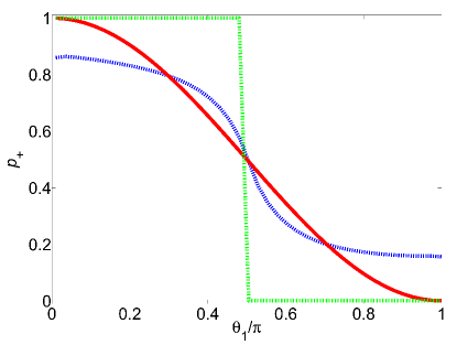
Figure 3: Noise. The probability $p_{+}$ is plotted as a function of the angle $\theta_{1}=\cos^{-1}\left(\mathbf{\hat{n}}_{1}\cdot\mathbf{\hat{u}}_{\mathrm{d}}\right)$ for the noiseless case (green dash-dotted line), the case $\phi_{0}=0.5$ (blue dashed line), and the Born rule (red solid line).

The measurement time - For the examples shown in Fig. 1, initially at time $t=0$, the ket vector $\left|\psi\right\rangle$ represents a product state having single-spin purity $P=1$. The time dependency of $P$ is shown in Fig. 1(b1), (b2), (b3) and (b4). In the short time limit of $\omega_{\mathrm{d}}t\ll 1$ the effect of the disentanglement term in the modified Schrödinger equation (4) is relatively weak (since $\left\langle\mathcal{Q}\right\rangle$ is initially small), and consequently $P$ rapidly drops due to entanglement generated by the dipolar interaction $V_{\mathrm{d}}$. At latter times, when disentanglement becomes sufficiently efficient, the single-spin purity $P$ starts increasing. Interaction-induced generation of entanglement becomes inefficient when the spin 1/2 becomes nearly parallel or nearly anti-parallel to the dipolar unit vector $\mathbf{\hat{u}}_{\mathrm{d}}$, and consequently the single-spin purity $P$ approaches unity in the long time limit.

For sufficiently short times after turning on the interaction (i.e. after $t=0$), time evolution is dominated by the effect of the dipolar interaction. When the effect of the disentanglement term is disregarded, one finds that in the short time limit the following holds $\mathrm{d}\left\langle\mathbf{S}_{n}\right\rangle/\mathrm{d}t\simeq\omega_{n}\mathbf{\hat{u}}_{\mathrm{d}}\times\left\langle\mathbf{S}_{n}\right\rangle$, where $n\in\left\{1,2\right\}$, $\omega_{1}=\omega_{\mathrm{d}}\hbar^{-1}\left\langle\mathbf{S}_{2}\cdot\mathbf{\hat{u}}_{\mathrm{d}}\right\rangle$ and $\omega_{2}=\omega_{\mathrm{d}}\hbar^{-1}\left\langle\mathbf{S}_{1}\cdot\mathbf{\hat{u}}_{\mathrm{d}}\right\rangle$. Thus, in the short time limit, the purity $P$ is roughly given by $P\simeq 1-\left(2^{-3/2}S_{2}\left|\mathbf{\hat{n}}_{1}\times\mathbf{\hat{u}}_{\mathrm{d}}\right|\left(\mathbf{\hat{n}}_{2}\cdot\mathbf{\hat{u}}_{\mathrm{d}}\right)\omega_{\mathrm{d}}t\right)^{2}$ [see Eqs. (6.192) and (8.701) of Ref. Buks_QMLN , and note that it is assumed that in the short time limit the spin states are nearly spin coherent states Radcliffe_313 ]. The above-derived expression for the purity time evolution $P\left(t\right)$ reveals the dependence of short-time dynamics on the macroscopicity of the measuring apparatus (i.e. the second spin), which is represented by the spin number $S_{2}$.

Vanishing Hamiltonian - To gain further insight into the disentanglement process generated by the nonlinear term $-\gamma\left(\mathcal{Q}-\left\langle\mathcal{Q}\right\rangle\right)$ added to the Schrödinger equation (4), consider for simplicity the case where the Hamiltonian vanishes, i.e. $\mathcal{H}=0$. The Schmidt decomposition of a general state vector $\left|\psi\right\rangle$ is expressed as

$$\left|\psi\right\rangle={\displaystyle\sum\limits_{l=1}^{\min\left(N_{1},N_{2}\right)}}q_{l}\left|l,l\right\rangle\;,$$ (7)

where $q_{l}$ are non-negative real numbers, the tensor product$\ \left|l\right\rangle_{1}\otimes\left|l\right\rangle_{2}$ is denoted by $\left|l,l\right\rangle\$, and $\left\{\left|l\right\rangle_{1}\right\}$ ($\left\{\left|l\right\rangle_{2}\right\}$) is an orthonormal basis spanning the Hilbert space of subsystem ’1’ (’2’). Note that for a product state $q_{l}=\delta_{l,l_{0}}$, where $l_{0}\in\left\{1,2,\cdots,\min\left(N_{1},N_{2}\right)\right\}$. The normalization condition reads $\left\langle\psi\right.\left|\psi\right\rangle=L_{2}=1$, where the $n$’th moment $L_{n}$ is defined by

$$L_{n}={\displaystyle\sum\limits_{l=1}^{\min\left(N_{1},N_{2}\right)}}q_{l}^{n}\;.$$ (8)

Note that for a product state $L_{n}=1$ for any positive integer $n$ (provided that $\left|\psi\right\rangle$ is normalized).

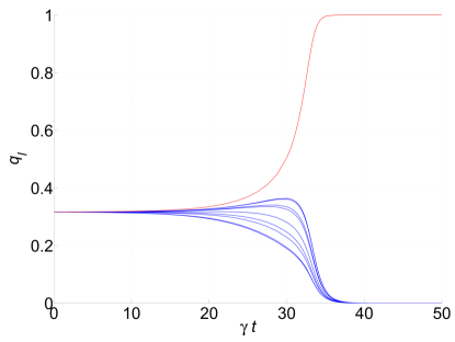
Figure 4: Vanishing Hamiltonian. The plot shows an example solution of the set of equations (10) for the case $\min\left(N_{1},N_{2}\right)=10$ and $\gamma=1$. The solution for $q_{l_{0}}\left(t\right)$ is represented by the red line, whereas the blue lines represent the solutions for $q_{l}\left(t\right)$ with $l\neq l_{0}$. For this example, $q_{l}\left(t=0\right)\simeq\left(\min\left(N_{1},N_{2}\right)\right)^{-1/2}$, i.e. the initial value of the purity $P$ is close to its smallest possible value of $1/\min\left(N_{1},N_{2}\right)$. The corresponding initial entropy $\sigma$ is close to its largest possible value of $\log\left(\min\left(N_{1},N_{2}\right)\right)$. In the limit $t\rightarrow\infty$ the purity $P\rightarrow 1$ (largest possible value) and the entropy $\sigma\rightarrow 0$ (smallest possible value).

In the Schmidt basis, the following holds [see Eqs. (2) and (3)]

$$\mathcal{Q}\left|\psi\right\rangle={\displaystyle\sum\limits_{l=1}^{\min\left(N_{1},N_{2}\right)}}q_{l}\left(1-q_{l}^{2}\right)\left|l,l\right\rangle\;,$$ (9)

and $\left\langle\mathcal{Q}\right\rangle=1-L_{4}$, and thus [see Eq. (4)]

$$\frac{\mathrm{d\log}q_{l}}{\mathrm{d}t}=\gamma\left(q_{l}^{2}-L_{4}\right)\;.$$ (10)

An example solution of the set of equations (10) for the case $\min\left(N_{1},N_{2}\right)=10$ and $\gamma=1$ is shown in Fig. 4.

The time evolution of the $n$’th moment $L_{n}$ is governed by [see Eqs. (8) and (10)]

$$\frac{\mathrm{d}L_{n}}{\mathrm{d}t}=n\gamma\left(L_{n+2}-L_{n}L_{4}\right)\;.$$ (11)

For the case of $n=2$, Eq. (11) yields the norm conservation condition $0=\left(\mathrm{d}/\mathrm{d}t\right)\left\langle\psi\right.\left|\psi\right\rangle$, which is satisfied provided that $\left|\psi\right\rangle$ is normalized, i.e. $L_{2}=1$ [see Eq. (7)]. For the case $n=4$ Eq. (11) yields an evolution equation for the purity $P=L_{4}$, which is given by $\mathrm{d}L_{4}/\mathrm{d}t=4\gamma\left(L_{6}-L_{4}^{2}\right)$. Using the Cauchy–Schwarz inequality one finds that $L_{4}^{2}\leq L_{2}L_{6}$ [see Eq. (8)], hence $\mathrm{d}P/\mathrm{d}t\geq 0$ (recall the normalization condition $L_{2}=1$), i.e. the purity $P$ monotonically increases with time. The same conclusion can alternatively be drawn from Eq. (10), which can be expressed as $\mathrm{d}q_{l}/\mathrm{d}t=\partial H/\partial q_{l}$, where $H=\left(\gamma/4\right)\left(3-2L_{2}\right)L_{4}$ [see Eq. (8), and note that $H=\left(\gamma/4\right)L_{4}=\left(\gamma/4\right)P$ when $L_{2}=1$].

For any two integers $l^{\prime},l^{\prime\prime}\in\left\{1,2,\cdots,\min\left(N_{1},N_{2}\right)\right\}$ the following holds [see Eq. (10)]

$$\frac{\mathrm{d\log}\frac{q_{l^{\prime}}}{q_{l^{\prime\prime}}}}{\mathrm{d}t}=\gamma\left(q_{l^{\prime}}^{2}-q_{l^{\prime\prime}}^{2}\right)\;.$$ (12)

The above relation (12) implies that the ratio $q_{l^{\prime}}/q_{l^{\prime\prime}}$ monotonically increases with time, provided that $q_{l^{\prime}}>q_{l^{\prime\prime}}$ (recall that $\gamma>0$). This behavior gives rise to disentanglement. Consider the case where initially, at time $t=0$, $q_{l_{0}}=\max\left\{q_{l}\right\}$ for a unique positive integer $l_{0}\in\left\{1,2,\cdots,\min\left(N_{1},N_{2}\right)\right\}$. For this case, $\left|\psi\right\rangle$ evolves into the product state $\left|l_{0},l_{0}\right\rangle$ in the long time limit, i.e. $q_{l}\rightarrow\delta_{l,l_{0}}$ in the limit $t\rightarrow\infty$ (see Fig. 4). Note, however, that in the long time limit the state can be strongly affected by noise when initially the set $\left\{q_{l}\right\}$ doesn’t have a unique member significantly larger than all others.

Discussion - As was already mentioned above, several types of nonlinear extensions of quantum mechanics have been proposed and explored Bassi_471 ; Bennett_170502 ; Kowalski_1 ; Fernengel_385701 ; Kowalski_167955 . However, it was found that for some cases, the proposed nonlinear extension gives rise to the violation of the causality principle by enabling superluminal signaling Bassi_055027 ; Jordan_022101 ; Polchinski_397 ; Helou_012021 . More recently, it was shown that when a condition called ’convex quasilinearity’ is satisfied by a given nonlinear master equation, the violation of the causality principle becomes impossible Rembielinski_012027 ; Rembielinski_420 . Some of the proposed nonlinear extensions are inconsistent with the principle of separability Hejlesen_thesis ; Jordan_022101 ; Jordan_012010 . Moreover, any proposed extension must be ruled out if it alters predictions of standard quantum mechanics that have been experimentally confirmed.

The modified Schrödinger equation given by Eq. (4) has an important advantage compared to other proposals: the added nonlinear term $-\gamma\left(\mathcal{Q}-\left\langle\mathcal{Q}\right\rangle\right)$ has no effect on product states. This implies that in the absence of entanglement, the added term does not vary any prediction of standard quantum mechanics. Moreover, possible conflicts with both principles of causality and separability can be avoided by postulating that $\gamma\simeq\hbar^{-1}\left\langle\psi\right|V^{{\dagger}}V\left|\psi\right\rangle^{1/2}$, where $V$ is the coupling term in the Hamiltonian giving rise to the interaction between subsystems [$\gamma$ is the disentanglement rate in Eq. (4)]. This postulate implies that the added nonlinear term is active only when subsystems interact, and that time evolution is governed by the standard Schrödinger equation when subsystems are remote (i.e. decoupled). Note that for the examples shown in Fig. 1, the calculations are performed for the case $\gamma=\omega_{\mathrm{d}}$. This demonstrates that a disentanglement rate $\gamma$ having the order of $\hbar^{-1}\left\langle\psi\right|V^{{\dagger}}V\left|\psi\right\rangle^{1/2}$ is sufficiently large to allow full suppression of entanglement.

Summary - Further theoretical study is needed to check whether quantum mechanics can be self-consistently reformulated based on the proposed modified Schrödinger equation (4). We find that conflict with some well-established physical principles, as well as many experimental observations, can be avoided by postulating that $\gamma\simeq\hbar^{-1}\left\langle\psi\right|V^{{\dagger}}V\left|\psi\right\rangle^{1/2}$.

The expression given by Eq. (2) for the operator $\mathcal{Q}$ is applicable for the bipartite case, for which the entire system is divided into two subsystems. The multipartite case, however, for which the entire system is divided into more than two subsystems, requires a generalization of Eq. (2). Such generalization is discussed in Ref. Buks_2306_05853 . The generalization of the above discussed postulate (regarding the disentanglement rate $\gamma$) for the multipartite case states that disentanglement between two given subsystems is active only during the time when they interact.

Further insight can be gained from experimental study of entanglement in the region where environmental decoherence is negligible Buks_014421 . Upper bounds imposed upon the disentanglement rate $\gamma$ in Eq. (4) can be derived from lifetime measurements of entangled states. Experimental observations of deviation from the Born rule may provide supporting evidence for nonlinearity (see Fig. 3).

Acknowledgments - We thank Jakub Rembielinski, Pawel Caban, Joakim Bergli and Klaus Molmer for useful discussions. This work was supported by the Israeli science foundation, the Israeli ministry of science, and by the Technion security research foundation.

Appendix A The Schmidt decomposition

The system’s normalized pure state vector $\left|\psi\right\rangle$ is given by $\left|\psi\right\rangle=\mathcal{K}_{1}C\otimes\mathcal{K}_{2}^{\mathrm{T}}$ [see Eq. (1) in the main text]. Consider the unitary transformations (the letter $k$ is used to label the states of the original basis, whereas the transformed states are labeled by the letter $l$)

$$\mathcal{K}_{1}^{\mathrm{T}} =u_{1}\mathcal{L}_{1}^{\mathrm{T}}=u_{1}\left(\left|l_{1}\right\rangle_{1},\left|l_{2}\right\rangle_{1},\cdots,\left|l_{N_{1}}\right\rangle_{1}\right)^{\mathrm{T}}\;,$$ (13)

$$\mathcal{K}_{2}^{\mathrm{T}} =u_{2}\mathcal{L}_{2}^{\mathrm{T}}=u_{2}\left(\left|l_{1}\right\rangle_{2},\left|l_{2}\right\rangle_{2},\cdots,\left|l_{N_{2}}\right\rangle_{2}\right)^{\mathrm{T}}\;,$$ (14)

where $u_{1}$ ($u_{2}$) is a $N_{1}\times N_{1}$ ($N_{2}\times N_{2}$) unitary matrix (i.e. $u_{1}^{{\dagger}}u_{1}=1$ and $u_{2}^{{\dagger}}u_{2}=1$). The state vector $\left|\psi\right\rangle$ in the transformed basis is expressed as

$$\left|\psi\right\rangle =\mathcal{L}_{1}\hat{C}\otimes\mathcal{L}_{2}^{\mathrm{T}}$$

$$={\displaystyle\sum\limits_{l_{1},l_{2}}}\hat{C}_{l_{1},l_{2}}\left|l_{1}\right\rangle_{1}\otimes\left|l_{2}\right\rangle_{2}\;,$$

(15)

where the transformed matrix $\hat{C}$ is given by

$$\hat{C}=u_{1}^{\mathrm{T}}Cu_{2}\;,$$ (16)

and the corresponding density operator $\rho=\left|\psi\right\rangle\left\langle\psi\right|$ is expressed as

$$\rho={\displaystyle\sum\limits_{l_{1}^{\prime},l_{2}^{\prime},l_{1}^{\prime\prime},l_{2}^{\prime\prime}}}\hat{C}_{l_{1}^{\prime},l_{2}^{\prime}}\hat{C}_{l_{1}^{\prime\prime},l_{2}^{\prime\prime}}^{\ast}\left|l_{1}^{\prime},l_{2}^{\prime}\right\rangle\left\langle l_{1}^{\prime\prime},l_{2}^{\prime\prime}\right|\;.$$ (17)

The following holds

$$\operatorname{Tr}\rho ={\displaystyle\sum\limits_{l_{1},l_{2}}}\left|\hat{C}_{l_{1},l_{2}}\right|^{2}$$

$$=\operatorname{Tr}S_{1}=\operatorname{Tr}S_{2}=\operatorname{Tr}\left(CC^{{\dagger}}\right)=\operatorname{Tr}\left(C^{{\dagger}}C\right)\;,$$

(18)

where the $N_{1}\times N_{1}$ ($N_{2}\times N_{2}$) matrix $S_{1}$ ($S_{2}$) is given by (recall that $u_{1}^{{\dagger}}u_{1}=1$ and $u_{2}^{{\dagger}}u_{2}=1$)

$$S_{1} =\hat{C}\hat{C}^{{\dagger}}=u_{1}^{\mathrm{T}}Cu_{2}u_{2}^{{\dagger}}C^{{\dagger}}u_{1}^{\mathrm{T{\dagger}}}=u_{1}^{\mathrm{T}}CC^{{\dagger}}u_{1}^{\mathrm{T{\dagger}}}\;,$$ (19)

$$S_{2} =\hat{C}^{{\dagger}}\hat{C}=u_{2}^{{\dagger}}C^{{\dagger}}u_{1}^{\mathrm{T{\dagger}}}u_{1}^{\mathrm{T}}Cu_{2}=u_{2}^{{\dagger}}C^{{\dagger}}Cu_{2}\;,$$ (20)

hence $\operatorname{Tr}\rho=1$ provided that $\left|\psi\right\rangle$ is normalized. The matrix $S_{1}$ ($S_{2}$) is Hermitian and positive definite, hence the unitary matrix $u_{1}$ ($u_{2}$) can be chosen to diagonalize $S_{1}$ ($S_{2}$), and the eigenvalues, which are denoted by $q_{l}$, are non-negative. For this transformation, which is called the Schmidt decomposition, the transformed matrix $\hat{C}$ has a diagonal form

$$\hat{C}_{l_{1},l_{2}}=q_{l_{1}}\delta_{l_{1},l_{2}}\;.$$ (21)

The purity $P_{1}$ ($P_{2}$) is defined by $P_{1}=\operatorname{Tr}\rho_{1}^{2}$ ($P_{2}=\operatorname{Tr}\rho_{2}^{2}$), where $\rho_{1}=\operatorname{Tr}_{2}\rho$ ($\rho_{2}=\operatorname{Tr}_{1}\rho$) is the reduced density operator of the first (second) subsystem. With the help of the Schmidt decomposition (21), one finds that $P_{1}=P_{2}\equiv P$, where

$$P ={\displaystyle\sum\limits_{l}}q_{l}^{4}$$

$$=\operatorname{Tr}S_{1}^{2}=\operatorname{Tr}\left(CC^{{\dagger}}\right)^{2}=\operatorname{Tr}S_{2}^{2}=\operatorname{Tr}\left(C^{{\dagger}}C\right)^{2}\;.$$

Note that $P=1\$for a product state, and $P$ obtains its minimum value of $1/\min\left(N_{1},N_{2}\right)$ for a maximally entangled state. The purity $P$ is independent on the local transformations $u_{1}$ and $u_{2}$, hence it is a constant when the subsystems are decoupled (i.e. when the interaction between the subsystems vanishes). Using the relations

$$\operatorname{Tr}\left(C^{{\dagger}}C\right)={\displaystyle\sum\limits_{k_{1}^{\prime}=1}^{N_{1}}}{\displaystyle\sum\limits_{k_{2}^{\prime}=1}^{N_{2}}}C_{{}_{k_{1}^{\prime},k_{2}^{\prime}}}^{\ast}C_{{}_{k_{1}^{\prime},k_{2}^{\prime}}}\;,$$ (23)

and

$$\operatorname{Tr}\left(C^{{\dagger}}C\right)^{2} ={\displaystyle\sum\limits_{k_{1}^{\prime},k_{1}^{\prime\prime}=1}^{N_{1}}}{\displaystyle\sum\limits_{k_{2}^{\prime},k_{2}^{\prime\prime}=1}^{N_{2}}}C_{k_{1}^{\prime},k_{2}^{\prime}}^{\ast}C_{k_{1}^{\prime},k_{2}^{\prime\prime}}C_{k_{1}^{\prime\prime},k_{2}^{\prime\prime}}^{\ast}C_{k_{1}^{\prime\prime},k_{2}^{\prime}}\;,$$

one finds that the level of entanglement $1-P$ is given by

$$1-P =\left(\operatorname{Tr}\left(C^{{\dagger}}C\right)\right)^{2}-\operatorname{Tr}\left(C^{{\dagger}}C\right)^{2}$$

$$=\frac{1}{2}{\displaystyle\sum\limits_{k_{1}^{\prime},k_{1}^{\prime\prime}=1}^{N_{1}}}{\displaystyle\sum\limits_{k_{2}^{\prime},k_{2}^{\prime\prime}=1}^{N_{2}}}\left|\phi_{k_{1}^{\prime},k_{1}^{\prime\prime},k_{2}^{\prime},k_{2}^{\prime\prime}}\right|^{2}\;,$$

(25)

where

$$\phi_{k_{1}^{\prime},k_{1}^{\prime\prime},k_{2}^{\prime},k_{2}^{\prime\prime}}=C_{{}_{k_{1}^{\prime},k_{2}^{\prime}}}C_{{}_{k_{1}^{\prime\prime},k_{2}^{\prime\prime}}}-C_{k_{1}^{\prime},k_{2}^{\prime\prime}}C_{k_{1}^{\prime\prime},k_{2}^{\prime}}\;.$$ (26)

Note that the term $\phi_{k_{1}^{\prime},k_{1}^{\prime\prime},k_{2}^{\prime},k_{2}^{\prime\prime}}$ vanishes unless $k_{1}^{\prime}\neq k_{1}^{\prime\prime}$ and $k_{2}^{\prime}\neq k_{2}^{\prime\prime}$, and the following holds $\phi_{k_{1}^{\prime},k_{1}^{\prime\prime},k_{2}^{\prime},k_{2}^{\prime\prime}}=\phi_{k_{1}^{\prime\prime},k_{1}^{\prime},k_{2}^{\prime\prime},k_{2}^{\prime}}$, thus Eq. (25) can be rewritten as

$$1-P=2{\displaystyle\sum\limits_{k_{1}^{\prime}<k_{1}^{\prime\prime}}}{\displaystyle\sum\limits_{k_{2}^{\prime}<k_{2}^{\prime\prime}}}\left|\phi_{k_{1}^{\prime},k_{1}^{\prime\prime},k_{2}^{\prime},k_{2}^{\prime\prime}}\right|^{2}\;.$$ (27)

Note that for any product state $\phi_{k_{1}^{\prime},k_{1}^{\prime\prime},k_{2}^{\prime},k_{2}^{\prime\prime}}=0$ [see Eq. (26)]. The above result (27) implies that $P=1-\left\langle\mathcal{Q}\right\rangle$, where the operator $\mathcal{Q}$ is given by Eq. (2) in the main text.

References

• (1) E. Schrodinger, “Die gegenwartige situation in der quantenmechanik”, Naturwissenschaften, vol. 23, pp. 807, 1935.
• (2) Roger Penrose, “Uncertainty in quantum mechanics: faith or fantasy?”, Philosophical Transactions of the Royal Society A: Mathematical, Physical and Engineering Sciences, vol. 369, no. 1956, pp. 4864–4890, 2011.
• (3) A. J. Leggett, “Experimental approaches to the quantum measurement paradox”, Found. Phys., vol. 18, pp. 939–952, 1988.
• (4) A. J. Leggett, “Realism and the physical world”, Rep. Prog. Phys., vol. 71, pp. 022001, 2008.
• (5) Eyal Buks, “Disentanglement and a nonlinear schrödinger equation”, Journal of Physics A: Mathematical and Theoretical, vol. 55, no. 35, pp. 355303, 2022.
• (6) Eyal Buks, “Thermalization and disentanglement with a nonlinear schrödinger equation”, in J. Phys. A: Math. Theor., 2023, vol. 56, p. 025302.
• (7) Michael R Geller, “Fast quantum state discrimination with nonlinear positive trace-preserving channels”, Advanced Quantum Technologies, p. 2200156, 2023.
• (8) Steven Weinberg, “Testing quantum mechanics”, Annals of Physics, vol. 194, no. 2, pp. 336–386, 1989.
• (9) Steven Weinberg, “Precision tests of quantum mechanics”, in THE OSKAR KLEIN MEMORIAL LECTURES 1988–1999, pp. 61–68. World Scientific, 2014.
• (10) H-D Doebner and Gerald A Goldin, “On a general nonlinear schrödinger equation admitting diffusion currents”, Physics Letters A, vol. 162, no. 5, pp. 397–401, 1992.
• (11) H-D Doebner and Gerald A Goldin, “Introducing nonlinear gauge transformations in a family of nonlinear schrödinger equations”, Physical Review A, vol. 54, no. 5, pp. 3764, 1996.
• (12) Nicolas Gisin and Ian C Percival, “The quantum-state diffusion model applied to open systems”, Journal of Physics A: Mathematical and General, vol. 25, no. 21, pp. 5677, 1992.
• (13) David E Kaplan and Surjeet Rajendran, “Causal framework for nonlinear quantum mechanics”, Physical Review D, vol. 105, no. 5, pp. 055002, 2022.
• (14) Manuel H Muñoz-Arias, Pablo M Poggi, Poul S Jessen, and Ivan H Deutsch, “Simulating nonlinear dynamics of collective spins via quantum measurement and feedback”, Physical review letters, vol. 124, no. 11, pp. 110503, 2020.
• (15) Angelo Bassi, Kinjalk Lochan, Seema Satin, Tejinder P Singh, and Hendrik Ulbricht, “Models of wave-function collapse, underlying theories, and experimental tests”, Reviews of Modern Physics, vol. 85, no. 2, pp. 471, 2013.
• (16) Philip Pearle, “Reduction of the state vector by a nonlinear schrödinger equation”, Physical Review D, vol. 13, no. 4, pp. 857, 1976.
• (17) Gian Carlo Ghirardi, Alberto Rimini, and Tullio Weber, “Unified dynamics for microscopic and macroscopic systems”, Physical review D, vol. 34, no. 2, pp. 470, 1986.
• (18) Angelo Bassi and GianCarlo Ghirardi, “Dynamical reduction models”, Physics Reports, vol. 379, no. 5-6, pp. 257–426, 2003.
• (19) IJ Arnquist, FT Avignone III, AS Barabash, CJ Barton, KH Bhimani, E Blalock, B Bos, M Busch, M Buuck, TS Caldwell, et al., “Search for spontaneous radiation from wave function collapse in the majorana demonstrator”, Physical Review Letters, vol. 129, no. 8, pp. 080401, 2022.
• (20) Eyal Buks, Quantum mechanics - Lecture Notes, http://buks.net.technion.ac.il/teaching/, 2023.
• (21) William K Wootters, “Entanglement of formation of an arbitrary state of two qubits”, Physical Review Letters, vol. 80, no. 10, pp. 2245, 1998.
• (22) JM Radcliffe, “Some properties of coherent spin states”, Journal of Physics A: General Physics, vol. 4, no. 3, pp. 313, 1971.
• (23) Charles H Bennett, Debbie Leung, Graeme Smith, and John A Smolin, “Can closed timelike curves or nonlinear quantum mechanics improve quantum state discrimination or help solve hard problems?”, Physical review letters, vol. 103, no. 17, pp. 170502, 2009.
• (24) Krzysztof Kowalski, “Linear and integrable nonlinear evolution of the qutrit”, Quantum Information Processing, vol. 19, no. 5, pp. 1–31, 2020.
• (25) Bernd Fernengel and Barbara Drossel, “Bifurcations and chaos in nonlinear lindblad equations”, Journal of Physics A: Mathematical and Theoretical, vol. 53, no. 38, pp. 385701, 2020.
• (26) K Kowalski and J Rembieliński, “Integrable nonlinear evolution of the qubit”, Annals of Physics, vol. 411, pp. 167955, 2019.
• (27) Angelo Bassi and Kasra Hejazi, “No-faster-than-light-signaling implies linear evolution. a re-derivation”, European Journal of Physics, vol. 36, no. 5, pp. 055027, 2015.
• (28) Thomas F. Jordan, “Assumptions that imply quantum dynamics is linear”, Phys. Rev. A, vol. 73, pp. 022101, Feb 2006.
• (29) Joseph Polchinski, “Weinberg?s nonlinear quantum mechanics and the einstein-podolsky-rosen paradox”, Physical Review Letters, vol. 66, no. 4, pp. 397, 1991.
• (30) Bassam Helou and Yanbei Chen, “Extensions of born?s rule to non-linear quantum mechanics, some of which do not imply superluminal communication”, in Journal of Physics: Conference Series. IOP Publishing, 2017, vol. 880, p. 012021.
• (31) Jakub Rembieliński and Paweł Caban, “Nonlinear evolution and signaling”, Physical Review Research, vol. 2, no. 1, pp. 012027, 2020.
• (32) Jakub Rembieliński and Paweł Caban, “Nonlinear extension of the quantum dynamical semigroup”, Quantum, vol. 5, pp. 420, 2021.
• (33) Zakarias Laberg Hejlesen, “Nonlinear quantum mechanics”, Master’s thesis, 2019.
• (34) Thomas F Jordan, “Why quantum dynamics is linear”, in Journal of Physics: Conference Series. IOP Publishing, 2009, vol. 196, p. 012010.
• (35) Eyal Buks, “Partial disentanglement in a multipartite system”, arXiv:2306.05853, 2023.
• (36) Eyal Buks and Banoj Kumar Nayak, “Quantum measurement with recycled photons”, Physical Review B, vol. 105, no. 1, pp. 014421, 2022.