Trust your source: quantifying source condition elements for variational regularisation methods

Abstract

Source conditions are a key tool in variational regularisation to derive error estimates and convergence rates for ill-posed inverse problems. In this paper, we provide a recipe to practically compute source condition elements as the solution of convex minimisation problems that can be solved with first-order algorithms. We demonstrate the validity of our approach by testing it for two inverse problem case studies in machine learning and image processing: sparse coefficient estimation of a polynomial via LASSO regression and recovering an image from a subset of the coefficients of its Fourier transform. We further demonstrate that the proposed approach can easily be modified to solve the machine learning task of identifying the optimal sampling pattern in the Fourier domain for given image and variational regularisation method, which has applications in the context of sparsity promoting reconstruction from magnetic resonance imaging data.

1 Introduction

Over the past decades, variational regularisation methods have been extensively used to approximate the solution of ill-posed inverse problems [46, 4]. The canonical example of an ill-posed inverse problem is the linear operator equation

$$Ku^{{\dagger}}=f$$ (1)

where $u^{{\dagger}}\in X$ is the quantity we wish to recover from the data $f\in Y$, and $K:X\rightarrow Y$ is a (linear) operator between functional spaces. In most practical applications, $f$ is not accessible; instead, we only have access to a perturbed version $f^{\delta}\in Y$. The key idea of variational regularisation methods consists of approximating $u^{{\dagger}}$ in (1) as the solution of the minimisation problem

$$\operatorname*{\arg\min}_{u\in X}\left\{\mathcal{D}(Ku,f^{\delta})+\alpha J(u)\right\},$$ (2)

where $\mathcal{D}(Ku,f^{\delta})$ is a data fidelity term ensuring that the minimiser $u_{\alpha}$ is close to the solution of (1), $J(u)$ is a regularisation functional favouring a-priori information of the solution or, equivalently, penalising solutions with undesired structures, and $\alpha>0$ is the regularisation parameter controlling the influence of the two terms on the minimiser. In this work, the data fidelity term is simply the least-squares term $\mathcal{D}(Ku,f^{\delta})=\frac{1}{2}\|Ku-f^{\delta}\|_{Y}^{2}$, motivated by assuming an additive Gaussian noise distribution of the data. The choice of the regularisation term is less straightforward and it has been an active field of research: from the pioneering work of Tikhonov [52, 53], to more recent papers on sparsity promoting regularisation [22, 17, 21], passing through the seminal work of Rudin et al. [45] and Mumford and Shah [40] where nonlinear variational models were first introduced. We want to emphasise that the concepts of inverse problems and variational regularisation also play a key role in machine learning tasks such as regression and logistic regression, with the LASSO [51] being one of the most prominent examples of a sparsity-promoting regression approach of the form of (2).

One reason for the popularity of variational regularisation methods is that, along with an intuitive approach to modelling, these provide a framework for their basic analysis, particularly in the case of convex regularisation functionals. In this context, once the existence of a minimiser for (2) is guaranteed by suitable assumptions of the functional, a compelling matter is establishing conditions to derive error estimates and quantify rates of convergence. These are generally smoothness conditions on the solution which go under the name of source conditions.

There exists several different types of source conditions and a detailed survey on the role of source conditions to derive convergence rates can be found in [48, Chapter 3]. Classical source conditions for nonlinear variation methods trace back to [20] and the seminal work of Burger and Osher [15], where the authors derive convergence rates in the Bregman distance [8] setting for general convex functionals in Banach spaces, extending the results already known in the quadratic case [23]. By that time, convergence rates under source conditions were established in the Hilbert setting [50], also for the nonlinear case [24].

An alternative – but often equivalent (see [4, Theorem 5.12]) – formulation to classical source conditions is provided by range conditions (see [15, Proposition 1] and [4, Definition 5.8]), which ensure that the unknown solution $u^{{\dagger}}$ of the inverse problem (1) is in the range of the variational regularisation operator. For example, range conditions (together with a restricted injectivity assumption) allow to establish linear converge rate for $\ell^{1}$ regularisation, avoiding stronger assumptions like the restricted isometry property [31]. More recently, range conditions have also been deployed in the context of data-driven regularisation [39].

While we will focus on source and range conditions in this work, we want to emphasise that stronger source conditions exists (like those in [44]) that yield better convergences rates compared to those derived in [15]. Other noticeable source conditions formulated as a variational inequality (instead of an equation or inclusion) are the so-called variational source conditions first introduced in [35] in the context of nonlinear ill-posed inverse problems. These have been widely used to derive converge rates [25]: in particular, in the context of sparsity promoting regularisers [30, 37, 36]. Last but not least, approximate source conditions have been used to quantify errors of regularisation methods and were originally introduced in the Hilbert setting [34], but quickly adapted to the Banach space setting [32]. They are generally weaker compared to classical source conditions, but allow to measure effectively how well the range condition can be approximated [14].

Over the years, source conditions have been regarded as a purely theoretical tool to quantify converge rates. In the papers cited above, there is little or no discussion on practical problems or applications where source conditions are proven to be met. Even for simple (non-trivial) inverse problems, systematic numerical studies of convergence rates for which the solutions provably verify a source condition are rare. Such examples include [43], where the authors consider a convolution operator and show that the convergence rates derived in their work are only verified in the case of a solution fulfilling the source condition. In [2, Example 6.1 & Section 6.2.1], the authors compare their theoretical error estimates with the computational errors. In order to do so, they propose two inverse problem solutions of which one can be shown to analytically satisfy the source condition while the other violates it (Example 6.1), and numerically estimate a source condition element to verify error estimates (Section 6.2.1.). More recently, in the context of statistical inverse learning problems, in [9, 10] the authors derive convergence rates in expected Bregman distance, using both classical and approximate source conditions. These are numerically verified for a tomographic problem using a solution that fulfils the source condition. Another exception is the special case of generalised eigenfunctions and singular vectors, whose theoretical and numerical computation has attracted significant interest over previous years (cf. [3, 26, 27, 12, 13, 29, 47, 4, 28, 42, 7, 11] and references therein).

Motivated by the lack of a generic, practical strategy to reliably estimate source and range condition elements, in this paper we propose a novel approach to compute source condition elements as the solution of a convex and differentiable minimisation problem. We prove that the solution is equivalent to fulfilling a classic source (or range) condition when $K$ in (1) is injective. We demonstrate the validity of our strategy by testing it numerically for two case studies: the machine learning problem of sparse polynomial regression and the image processing problem of recovering an image from a subset of its Fourier sampels. Having at disposal explicit knowledge of the source condition elements has indubitable significance from a theoretical perspective: 1) the source condition element provides exact quantitative error estimates (i.e., the constants appearing in the convergence rates bounds can be computed explicitly), and 2) computing a range condition element allows us to determine the data that is required for a variational regularisation approach to reproduce the solution of an inverse problem. However, it also opens up interesting lines of research in the context of learning for inverse problems. In this work, we show how estimating a sparse source condition element can be used to devise a strategy for optimally sampling in the Fourier domain in the context of variational regularisation. Applications for such a problem can for instance be found in Magnetic Resonance Imaging (MRI) (cf. [49]).

Our contributions. The main contribution of this paper is a novel, practical approach to compute source conditions elements, with the aim of depicting the source conditions as quantitative tools in variational regularisation, rather than merely theoretical requirements. To do so, we consider a rather general Banach space setup, and we employ tools from convex analysis to provide an alternative formulation for the source condition, together with an iterative procedure for the numerical approximation of the source condition element. To demonstrate the potential of this strategy in practical applications, we provide a set of numerical experiments where we focus on two ill-posed inverse problem: 1D interpolation and 2D imaging. Finally, we show how the proposed approach can inspire optimal design techniques, by suitably sampling the forward operator to promote desired properties of the associated source condition elements.

Structure of the paper. The remainder of the paper is organised as follows. Section 2 is devoted to briefly reviewing relevant theoretical concepts from convex analysis. In Section 3, we describe what source conditions are, why they are necessary and detail the key idea of our approach, namely, how to compute source condition elements as the solution of a convex minimisation problem. We demonstrate the performance of our methodology by a series of numerical experiments in Section 4 with focus on machine learning. In particular, in Section 4.3 we show how our strategy can be used to learn the optimal sampling pattern in the Fourier domain for a fixed image and given variational regularisation method. Concluding remarks and future prospects are summarised in Section 5.

2 Mathematical preliminaries

In this section, we set the notation and give a brief overview of some key results from convex analysis which are useful for the rest of the paper (see [33]).

For a functional $F\colon X\rightarrow\mathbb{R}$, the subdifferential evaluated at a point $\hat{u}\in X$ is defined as

$$\partial F(\hat{u})=\big{\{}x^{*}\in X^{*}:F(u)-F(\hat{u})\geq\langle x^{*},u-\hat{u}\rangle_{*}\big{\}}.$$

If $F$ is also differentiable, the only element of the subgradient $\partial F(\hat{u})$ is $\nabla F(\hat{u})$.
The convex conjugate of a functional $F\colon X\rightarrow\mathbb{R}$ is defined as $F^{\star}\colon X^{*}\rightarrow\mathbb{R}$ such that

$$F^{\star}\colon p\in X^{*}\mapsto F^{\star}(p)=\sup_{u\in X}\left\{\langle p,u\rangle_{*}-F(u)\right\},$$

where $\langle\cdot,\cdot\rangle_{*}$ denotes the canonical pairing between the dual space $X^{*}$ and $X$. If $X$ is a Hilbert space, we can interpret $F^{\star}$ as a functional from $X$ to $\mathbb{R}$, by identifying $X$ with $X^{*}$ via the Riesz’s representation theorem.
For a continuous convex functional $F$, the Bregman distance between $u$ and $w$, associated with $p\in\partial F(w)$ is defined as

$$D_{F}^{p}(u,w)=F(u)-F(w)-\langle p,u-w\rangle_{*}.$$

Such a mapping is actually not a distance: it is non-negative but, in general, it is not symmetric and it does not satisfy the triangular inequality. To recover the symmetry, we usually rely on the symmetric Bregman distance, also known as the Jeffrey’s distance, namely:

$$D_{F}^{\text{symm},q,p}(u,w)=D_{F}^{q}(w,u)+D_{F}^{p}(u,w)\qquad q\in\partial F(u),\ p\in\partial F(w).$$

Notice that if $F$ is differentiable the subdifferentials are single-valued, hence we can drop the dependence from $p,q$ and simply denote by $D_{F}(u,w)$ the symmetric Bregman distance between $u$ and $w$.

3 Computing source condition elements

We consider the inverse problem (1) of recovering $u^{\dagger}\in X$ from $f^{\delta}\in Y$, a perturbation of the noiseless measurements $f=Ku^{\dagger}$ satisfying $\|f^{\delta}-f\|_{Y}\leq\delta$. The forward map $K\colon X\rightarrow Y$ is a bounded linear operator, but we allow it to be compact and hence, do not assume that it admits a bounded inverse in general. As a consequence, retrieving $u^{\dagger}$ from $f^{\delta}$ is an ill-posed problem, and solving (1) can suffer from instability in particular. The goal of regularisation theory for inverse problems is to construct a (family of) continuous operators that provide a satisfactory approximation of the potentially discontinuous inverse map. One of the most prominent paradigms is represented by variational regularisation, where a family of (potentially set-valued) operators $R_{\alpha}$, parameterised by $\alpha\in(0,\infty)$, is defined as

$$R_{\alpha}\colon Y\rightrightarrows X,\quad R_{\alpha}\colon f\mapsto u_{\alpha}\in\operatorname*{\arg\min}_{u\in X}\left\{\frac{1}{2}\|Ku-f\|_{Y}^{2}+\alpha J(u)\right\},$$ (3)

with $J\colon X\rightarrow\mathbb{R}\cup\{\infty\}$ being a so-called regularisation functional. For the remainder of this work, we make the following set of assumptions.

Assumption 3.1.

We require the following conditions to be satisfied:

• $Y$ is a Hilbert space;

• $X$ is the dual of a normed space $\mathcal{X}$ such that its weak-star topology on $X$ is metrisable on bounded sets;

• $K$ is the adjoint of a bounded linear operator from $Y$ to $\mathcal{X}$;

• $J$ is the conjugate of a proper functional from $\mathcal{X}$ to $\mathbb{R}\cup\{\infty\}$ and is non-negative;

• for every $f\in Y$ and $\alpha>0$ there exists a constant $c=c(a,b,\|f\|)$ that depends monotonically non-decreasing on all arguments such that $\|u\|_{X}\leq c$ if $\|Ku-f\|\leq a$ and $J(u)\leq b$.

Notice in particular that the assumption on $J$ implies that it is a convex functional. Under those assumptions, it is possible to prove that (3) is well defined: namely, that for every $f\in Y$ and $\alpha>0$ the set $R_{\alpha}(f)$ is non-empty (see [4, Theorem 5.6], which also shows that $R_{\alpha}(f)$ is convex). Moreover, for $\alpha>0$, each operator $R_{\alpha}$ is stable in the sense of the Kuratowski limit superior: namely, for every sequence $f_{n}\rightarrow f$ in $Y$ there exists a subsequence $u_{n_{k}}\in R_{\alpha}(f_{n_{k}})$ converging to an element $u^{*}\in R_{\alpha}(f)$ in the weak-star topology on $X$ (see [4, Theorem 5.7]). To conclude that $R_{\alpha}$ is a family of regularisers, one needs to ensure that, if the noise level $\delta$ converges to zero, i.e. $\delta\rightarrow 0$, there exists a choice $\alpha(\delta)$ such that $R_{\alpha(\delta)}(f^{\delta})$ converges to $u^{\dagger}$. More advanced results in this direction also provide convergence rates, usually at the price of an additional assumption involving the unknown solution $u^{\dagger}$. In particular, a pivotal tool to obtain quantitative error estimates between the solution $u^{\dagger}$ and the regularized solution $u_{\alpha}$ is represented by the source condition. In their most classical formulation, these accounts to assume that there exists $v\in Y$ such that

$$K^{\ast}v\in\partial J(u^{\dagger}),$$ (SC)

where $K^{\ast}\colon Y\rightarrow X^{*}$ is the adjoint of $K$ (thanks to Riesz representation lemma, we identify $Y$ with its dual), and $\partial J\subset X^{*}$ is the subdifferential of $J$ (see Section 2). The object $v\in Y$ is referred to as the source condition element: in the following, we want to recall why source condition elements enable us to derive error estimates with convergence rates strategies (Section 3.1) and then discuss how to compute $v$ for given $u^{\dagger}$, if such $v$ exists in Section 3.2.

3.1 Error estimates for variational regularisation methods

In [15, 4], error estimates measured in Bregman distances have been established for convex but non-smooth variational regularisation methods with the help of source conditions. For reasons of self-containment, we recall one of the key results. We start by an equivalent formulation of (3) by means of first-order optimality conditions, exploiting the convexity of $J$: namely, $u_{\alpha}\in R_{\alpha}(f^{\delta})$ if and only if

$$\exists\,p_{\alpha}\in\partial J(u_{\alpha}):\quad K^{\ast}(Ku_{\alpha}-f^{\delta})+\alpha p_{\alpha}=0\,,$$

where the previous equality holds in $X^{*}$. Assuming that (SC) is satisfied, we can subtract $\alpha K^{\ast}v$ on both sides of the equation to obtain

$$K^{\ast}(Ku_{\alpha}-f^{\delta})+\alpha\left(p_{\alpha}-K^{\ast}v\right)=-\alpha K^{\ast}v\,.$$

Taking a dual product of both sides of the equation with $u_{\alpha}-u^{\dagger}$ then yields

$$\langle Ku_{\alpha}-f^{\delta},Ku_{\alpha}-f\rangle_{Y}+\alpha\langle u_{\alpha}-u^{\dagger},p_{\alpha}-K^{\ast}v\rangle_{*}=-\alpha\langle K^{\ast}v,u_{\alpha}-u^{\dagger}\rangle_{*}\,.$$

Please note that $\langle\cdot,\cdot\rangle_{Y}$ indicates the inner product in $Y$, whereas $\langle\cdot,\cdot\rangle_{*}$ denotes the pairing between a functional in $X^{*}$ and an element of $X$. We can interpret the second term on the left-hand side by means of the symmetric Bregman distance. Since $p_{\alpha}\in\partial J(u_{\alpha})$ and $K^{\ast}v\in\partial J(u^{\dagger})$, the quantity $\langle u_{\alpha}-u^{\dagger},p_{\alpha}-K^{\ast}v\rangle_{*}$ equals $D_{J}^{\text{symm},p_{\alpha},K^{*}v}(u_{\alpha},u^{\dagger})$ (in the following we only refer to this term as $D_{J}^{\text{symm}}$ for ease of notation). In addition, we can reformulate $\langle Ku_{\alpha}-f^{\delta},Ku_{\alpha}-f\rangle_{Y}$ to

$$\langle Ku_{\alpha}-f+f-f^{\delta},Ku_{\alpha}-f\rangle_{Y}=\frac{1}{2}\|Ku_{\alpha}-f\|_{Y}^{2}+\frac{1}{2}\|Ku_{\alpha}-f^{\delta}\|_{Y}^{2}-\frac{1}{2}\|f-f^{\delta}\|_{Y}^{2},$$

to obtain

$$\frac{1}{2}\|Ku_{\alpha}-f\|_{Y}^{2}+\frac{1}{2}\|Ku_{\alpha}-f^{\delta}\|_{Y}^{2}+\alpha D_{J}^{\text{symm}}(u_{\alpha},u^{\dagger})=\frac{1}{2}\|f-f^{\delta}\|_{Y}^{2}-\alpha\langle v,Ku_{\alpha}-f\rangle_{Y}\,,$$

where we have made use of (1), which assumes the identity $Ku^{\dagger}=f$. Using the identity

$$\langle\alpha v,f-Ku_{\alpha}\rangle_{Y}=\frac{\alpha^{2}}{2}\|v\|_{Y}^{2}+\frac{1}{2}\|Ku_{\alpha}-f\|_{Y}^{2}-\frac{1}{2}\|\alpha v-f+Ku_{\alpha}\|_{Y}^{2}$$

and subsequently eliminating $\frac{1}{2}\|Ku_{\alpha}-f\|_{Y}^{2}$ on both sides leads to the equation leads to

$$\frac{1}{2}\|Ku_{\alpha}-f+\alpha v\|_{Y}^{2}+\frac{1}{2}\|Ku_{\alpha}-f^{\delta}\|_{Y}^{2}+\alpha D_{J}^{\text{symm}}(u_{\alpha},u^{\dagger})=\frac{1}{2}\|f-f^{\delta}\|_{Y}^{2}+\frac{\alpha^{2}}{2}\|v\|_{Y}^{2}\,.$$

Dividing by $\alpha$ and using the estimate $\|f-f^{\delta}\|_{Y}\leq\delta$ then yields the well-known error estimate (cf. [16])

$$\frac{1}{2\alpha}\|Ku_{\alpha}-f+\alpha v\|_{Y}^{2}+\frac{1}{2\alpha}\|Ku_{\alpha}-f^{\delta}\|_{Y}^{2}+D_{J}^{\text{symm}}(u_{\alpha},u^{\dagger})\leq\frac{\alpha}{2}\|v\|_{Y}^{2}+\frac{\delta^{2}}{2\alpha}\,.$$

With the a-priori choice $\alpha(\delta)=\delta/\|v\|_{Y}$ we minimise the right-hand-side of the inequality and obtain

$$\begin{split}0&\leq\frac{\|v\|_{Y}}{2\delta}\left\|Ku_{\alpha(\delta)}-f+\delta\frac{v}{\|v\|_{Y}}\right\|_{Y}^{2}+\frac{\|v\|_{Y}}{2\delta}\|Ku_{\alpha(\delta)}-f^{\delta}\|_{Y}^{2}+D_{J}^{\text{symm}}(u_{\alpha(\delta)},u^{\dagger})\\ &\leq\|v\|_{Y}\delta\,.\end{split}$$ (4)

Hence, the symmetric Bregman distance between $u_{\alpha(\delta)}$ and $u^{\dagger}$ is bounded by the worst-case data error bound $\delta$ multiplied by the norm of the source condition element $v$. To quantify a-priori error estimates such as (4) it is therefore vital to quantify the norm of the source condition element.

3.2 Casting the computation of source condition elements as convex minimisation problems

Having established the need for source condition elements and estimates for their norm in order to quantify a-priori error estimates of regularised inverse problems solutions, we now discuss how we can formulate the computation of $v$ verifying (SC) as a variational minimisation problem for a suitable convex and differentiable functional.
We first assume, in analogy to [16], that the space $X$ is continuously embedded into a Hilbert space $Z$. By means of the Hahn-Banach theorem, $K$ can be extended to a bounded linear operator from $Z$ to $Y$ (which, with an abuse of notation, we still denote as $K$), whereas we interpret the functional $J$ as acting on the whole space $Z$ by extending it to $\infty$ outside of $X$. By this modification, we can equivalently solve the minimisation problem (3) in $X$ or in $Z$.

Remark 3.1.

To rigorously verify the last statement, assume that $\tilde{K}\colon Z\rightarrow Y$ and $\tilde{J}\colon Z\rightarrow\mathbb{R}$ are the proposed extensions of $K$ and $J$. Then, for any $f\in Y$, the problem

$$\tilde{u}_{\alpha}\in\tilde{R}_{\alpha}(u)=\operatorname*{\arg\min}_{u\in Z}\left\{\frac{1}{2}\|\tilde{K}u-f\|_{Y}^{2}+\alpha\tilde{J}(u)\right\}$$

is such that $\tilde{R}_{\alpha}(f)=R_{\alpha}(f)$. Moreover, the optimality conditions are equivalent, since it is possible to show that, for $\hat{u}\in X$, the set $\partial\left\{\frac{1}{2}\|\tilde{K}\cdot-f\|_{Y}^{2}+\alpha\tilde{J}\right\}(\hat{u})\subset Z$ can be identified (via bounded extension) with the set $\partial\left\{\frac{1}{2}\|K\cdot-f\|_{Y}^{2}+\alpha J\right\}(\hat{u})\subset X^{*}$.

Motivated by [54], we provide a characterisation of the source condition element involving the use of proximity operators. For a proper, convex, lower semi-continuous functional $F$ defined on the Hilbert space $Z$, the proximity operator (or proximal map) is defined as

$$\operatorname{prox}_{F}\colon Z\rightarrow Z,\qquad\operatorname{prox}_{F}(z):=\operatorname*{\arg\min}_{u\in Z}\left\{\frac{1}{2}\|u-z\|_{Z}^{2}+F(u)\right\}\,.$$ (5)

The Hilbert space structure is, in principle, not needed for the definition of the proximal operator: for example, if $X$ is assumed to be a Banach space, its norm can be used inside (5), which would not lead to an equivalent operator. We nevertheless rely on definition (5) and on the use of the norm $\|\cdot\|_{Z}$. The following result provides an alternative formulation of (SC).

Proposition 3.1.

The source condition (SC) can be rewritten as

$$u^{\dagger}=\operatorname{prox}_{J}\left(u^{\dagger}+K^{\ast}v\right)\,,$$ (6)

Proof.

By Assumption 3.1, the functional $J$ is convex, which implies that $\frac{1}{2}\|\cdot-z\|_{Z}^{2}+J$ is strictly convex, for every $z\in Z$. Therefore, its minimiser can be determined by means of first-order optimality conditions, yielding

$$u=\operatorname{prox}_{J}(z)\quad\Leftrightarrow\quad z-u\in\partial J(u).$$ (7)

Choosing $u=u^{\dagger}$ and $z=u^{\dagger}+K^{*}v$ (since $K$ has been extended to an operator from $Z$ to $Y$, it holds $K^{*}\colon Y\rightarrow Z$), we conclude (6). ∎

The advantage of the Hilbert space structure mainly resides in the possibility to use the expression (7). In Banach spaces, a similar result holds, but it requires the use of duality mappings, which would prevent the development of the following results. From this moment on, for the ease of notation, we denote by $\|\cdot\|$ the norm on the Hilbert space $Z$, previously denoted as $\|\cdot\|_{Z}$, and as $\langle\cdot,\cdot\rangle$ the inner product in $Z$.

We now reformulate the source condition by means of the following functional, which, following [54], we refer to as the Bregman loss:

$$B_{J}(u,p):=\left(\frac{1}{2}\|\cdot\|^{2}+J\right)(u)+\left(\frac{1}{2}\|\cdot\|^{2}+J\right)^{\star}(p)-\langle p,u\rangle\,,$$ (8)

where $(\frac{1}{2}\|\cdot\|^{2}+J)^{\star}$ denotes the convex conjugate of $\frac{1}{2}\|\cdot\|^{2}+J$.

We provide a summary of results related to $B_{J}$, which provide possible interpretations as well as important properties which will be used later. A proof of the following Proposition can be found in [54, Theorem 10].

Proposition 3.2.

The functional $B_{J}\colon Z\times Z\rightarrow\mathbb{R}$ satisfies the following properties:

1. $B_{J}(u,p)=D_{\frac{1}{2}\|\cdot\|^{2}+J}^{p}(u,\operatorname{prox}_{J}(p))$;

2. $B_{J}(u,p)=\frac{1}{2}\|u-\operatorname{prox}_{J}(p)\|^{2}+D_{J}^{p-\operatorname{prox}_{J}(p)}(u,\operatorname{prox}_{J}(p))$;

3. $B_{J}$ is bi-convex (separately in the variables $u,p$);

4. for any fixed $u\in\operatorname{dom}(J)$, the function $B_{J}(u,\cdot)$ is continuously Fréchet-differentiable: in particular,

   $$\nabla_{p}B_{J}(u,p)=\operatorname{prox}_{J}(p)-u;$$

5. if moreover $\partial J(u)\neq\varnothing$, then $u=\operatorname{prox}_{J}(p)$ is a global minimiser of $B_{J}(u,\cdot)$.

Remark 3.2.

Note that, if $u\in\operatorname{dom}(J)$ but $J(u)=\varnothing$, an element $\hat{p}$ such that $\nabla_{p}B_{J}\left(u,\hat{p}\right)=0$ may not exist. This scenario never occurs if $u\in\operatorname{int}(\operatorname{dom}(J))$, and in particular when the domain of $J$ is a closed subset of $Z$.

In view of Proposition 3.2, we focus on the problem of minimising $B_{J}(u,\cdot)$ for a fixed $p$. According to $a)$ and $b)$, this accounts to finding an object $\hat{p}$ such that $\operatorname{prox}_{J}(\hat{p})$ is close to $u$ and in particular, if the minimum is attained that $u=\operatorname{prox}_{J}(\hat{p})$. Moreover, thanks to the convexity and Fréchet-differentiability of $B_{J}(u,\cdot)$, its minimisation of $B_{J}(u,\cdot)$ can be performed by means of first-order optimisation methods.

Combining ideas from Propositions 3.1 and 3.2, we introduce the functional

$$G_{J}\colon Y\rightarrow\mathbb{R},\quad G_{J}(v)=B_{J}(u^{\dagger},u^{\dagger}+K^{*}v).$$

Since $G_{J}$ is a composition of an affine map with $B_{J}(u^{\dagger},\cdot)$, it inherits the convexity and differentiability, and in particular

$$\nabla G_{J}(v)=K\operatorname{prox}_{J}(u^{\dagger}+K^{*}v)-Ku^{\dagger}.$$ (9)

We immediately deduce the following result, related to the source condition:

Proposition 3.3.

If there exists $v$ which satisfies (SC), then such $v$ is a global minimiser of $G_{J}$. Viceversa, if $v$ is a global minimiser of $G_{J}$, it satisfies

$$Ku^{\dagger}=K\operatorname{prox}_{J}\left(u^{\dagger}+K^{\ast}v\right),$$ (10)

which automatically implies (SC) if $K$ only has a trivial null space.

Remark 3.3.

Please note that Proposition 3.3 does not guarantee the existence of a global minimiser of $G_{J}$.

Remark 3.4.

We want to emphasise that if $K$ is injective and has a non-trivial null space, an element $v$ that sets (9) to zero can still satisfy (SC) as long as $\operatorname{prox}(u^{\dagger}+K^{\ast}v)-u^{\dagger}$ does not lie in the null space of $K$. Furthermore, we can always verify $v$ satisfies (SC) a-posteriori.

In order to check if $u^{\dagger}$ satisfies the source condition, and to compute the associated $v$, we are interested in solving

$$\hat{v}=\operatorname*{\arg\min}_{v}G_{J}(v)=\operatorname*{\arg\min}_{v}B_{J}\left(u^{\dagger},u^{\dagger}+K^{\ast}v\right)\,.$$

We can solve this minimisation problem with various different first-order methods, the simplest one being gradient descent. Thanks to (9), the iterative step in this case reads

$$v^{k+1}=v^{k}-\tau K\left(\text{prox}_{J}\left(u^{\dagger}+K^{\ast}v^{k}\right)-u^{\dagger}\right)\,,$$ (11)

which is globally convergent for $\tau\leq 1/\|K\|^{2}$ for arbitrary initial value $v^{0}\in Y$, since every proximal map is $1$-Lipschitz.

The descent algorithm described in (11) allows to approximate a source condition element by means of simple iterations. Nevertheless, it requires the knowledge of the proximal map $\operatorname{prox}_{J}$, which has a closed-form solution for many popular choices of the functional $J$. However, many interesting functionals do not have closed-form proximal maps, such as the popular class of functionals of the form $J(u)=H(Au)$, where $H$ is a functional with closed-form proximal map but where $A$ is a linear operator. In the next section, we provide a strategy to deal with this larger family of regularisation functionals. An alternative approach, at least from a numerical perspective, is to approximate the evaluation of $\operatorname{prox}_{J}$ by means of a suitable optimisation sub-routine.

3.3 Extension to more general functionals and range conditions

In this section, we consider composite functionals of the form

$$J(u)=H(Au+b)\,,$$ (12)

with $b\in Z$ and $A\colon Z\rightarrow Z$, and for which we assume that $\operatorname{prox}_{H}$ is known. This allows to take into account a large family of regularisation strategies, including generalised Tikhonov, sparsity promotion with respect to orthogonal bases or frames, and Total Variation, as we are going to recall in Section 4.2.

In order to estimate source condition elements in this scenario, we start by relating the source condition with the range condition. Referring to [4, Definition 4.9], we say that $u^{\dagger}$ satisfies the range condition for $\alpha>0$ if there exists data $g_{\alpha}\in Y$ such that

$$u^{\dagger}\in\operatorname*{\arg\min}_{u\in X}\left\{\frac{1}{2}\|Ku-g_{\alpha}\|^{2}+\alpha J(u)\right\}\,,$$ (RC1)

which means that $u^{\dagger}$ is in the range of the regulariser $R_{\alpha}$, which motivates the name of the assumption. Thanks to Assumption 3.1 and to the definition of $R_{\alpha}$ in (3), we can apply [4, Theorem 5.12] and conclude that $u^{\dagger}$ satisfies the range condition (RC1) for all $\alpha>0$ if and only if it verifies the source condition (SC). In particular, considering the equivalent optimality condition associated with (RC1),

$$\frac{1}{\alpha}K^{\ast}\left(g_{\alpha}-Ku^{\dagger}\right)\in\partial J(u^{\dagger})\,,$$ (RC2)

we immediately obtain the following expression connecting the source condition element $v$ with the pre-image $g_{\alpha}$:

$$g_{\alpha}=Ku^{\dagger}+\alpha v.$$ (13)

Even though this equivalence holds true for any feasible $J$, it is particularly useful when applied to functionals of the form (12). Indeed, in this case the range condition (RC2) can be written as

$$K^{\ast}(Ku^{\dagger}-g_{\alpha})+\alpha A^{\ast}q^{\dagger}=0\,,$$

for $q^{\dagger}\in\partial H(Au^{\dagger}+b)$. Multiplying by $1/\alpha$ and using (13) then yields the conditions

$$K^{\ast}v =A^{\ast}q^{\dagger}\,,$$ (14a)

$$q^{\dagger} \in\partial H(Au^{\dagger}+b)\,.$$ (14b)

In analogy to Section 3.2, we can rewrite (14b) as $Au^{\dagger}+b+q^{\dagger}\in\partial\left(\frac{1}{2}\|\cdot\|^{2}+H\right)(Au^{\dagger}+b)$, respectively $Au^{\dagger}+b=\operatorname{prox}_{H}(Au^{\dagger}+b+q^{\dagger})$, set up a Bregman loss functional and define the corresponding functional $G_{H}\colon Y\rightarrow\mathbb{R}$ as

$$G_{H}(q)=B_{H}(Au^{\dagger}+b,q+Au^{\dagger}+b)\,.$$

Then, we can formulate estimating the source condition element $v$ and the subgradient $q^{\dagger}$ as the minimisation of the objective functional

$$E_{H}(v,q^{\dagger})=\frac{1}{2}\|K^{\ast}v-A^{\ast}q^{\dagger}\|^{2}+G_{H}(q^{\dagger})\,.$$ (15)

Indeed, setting the partial Fréchet derivatives of (15) to zero yields

$$K\left(K^{\ast}v-A^{\ast}q^{\dagger}\right) =0\,,$$

$$A\left(A^{\ast}q^{\dagger}-K^{\ast}v\right)+\text{prox}_{H}\left(Au^{\dagger}+b+q^{\dagger}\right)-Au^{\dagger}-b =0\,.$$

The above expressions are not equivalent to the range condition (RC1). Nevertheless, as in Proposition 3.3, if we assume that $K$ has a trivial null space, then the first expression implies that (14a) is satisfied, whereas the second one implies (14b). Moreover, we can always check a-posteriori if $v$ and $q^{\dagger}$ satisfy (14).

In order to approximate a minimiser of $E_{H}$, we again can use first order methods. Since minimising (15) is a minimisation problem in two variables, it seems logical to use algorithms such as explicit coordinate descent [1, 55], i.e.

$$v^{k+1} =v^{k}-\tau K(K^{*}v^{k}-A^{*}q^{k})$$ (16)

$$q^{k+1} =q^{k}-\sigma\Big{(}A(A^{*}q^{k}-K^{*}v^{k+1})+\operatorname{prox}_{H}(Au^{\dagger}+b+q^{k})-Au^{\dagger}-b\Big{)},$$

which guarantees the (global) convergence to a minimiser, provided that the the step sizes $\sigma,\tau$ are suitably chosen. Alternatively, one can formulate the augmented Lagrangian

$$\mathcal{L}_{\delta}(v,q^{\dagger};\mu)=\frac{\delta}{2}\|K^{\ast}v-A^{\ast}q^{\dagger}\|^{2}+G_{H}(q^{\dagger})+\langle\mu,K^{\ast}v-A^{\ast}q^{\dagger}\rangle$$

and employ algorithmic approaches such as the alternating direction method of multipliers (ADMM) [38] and variants to find the saddle-point, or directly formulate the saddle-point problem

$$\inf_{v,q^{\dagger}}\sup_{\mu}G_{H}(q^{\dagger})+\langle\mu,K^{\ast}v-A^{\ast}q^{\dagger}\rangle$$

and compute the saddle-point with algorithms such as the primal-dual hybrid gradient method or variants of it (see [19, 5] and references therein).

In the following section, we provide some numerical examples to discuss the effectiveness of the reconstruction of source condition elements, both via the minimisation of $G_{J}$ or of $E_{H}$, according to the different choices of $J$.

4 Numerical results

In this section, we demonstrate the validity of our strategy by testing it for two case studies: in Subsection 4.1 we consider the machine learning problem of polynomial LASSO regression, while in Subsection 4.2 we consider the problem of estimating a two-dimensional image from a subset of its Fourier samples. Finally, in Subsection 4.3 we show how our strategy can be used to learn the optimal sampling pattern in the Fourier domain for a fixed image and given variational regularisation method.

4.1 1D example: Polynomial LASSO regression

As a first example, we show how to estimate source condition elements for a polynomial regression model. We start by considering the polynomial

$$\varphi(u)=5u^{2}-3u^{5}-1,$$ (17)

with $u\in\mathbb{R}$, and $\varphi:\mathbb{R}\rightarrow\mathbb{R}$. We assume that we cannot directly access $\varphi(u)$, but instead have $N$ pairs of samples $(u_{i},f^{\delta}_{i})$ for $i\in\{1,\ldots,N\}$ with

$$f^{\delta}_{i}=\varphi(u_{i})+\varepsilon_{i},\;\;\;\;\varepsilon_{i}\sim\mathcal{N}(0,\sigma^{2}),$$ (18)

i.e., measured data is affected by additive noise $\varepsilon_{i}$ sampled from a Gaussian distribution with zero mean and standard deviation $\sigma$, and the superscript $\delta$ refers to the resulting data error $\delta=\|f-f^{\delta}\|$. We choose $\sigma=0.1$ for our experiments and an example of sampled values is shown in Figure 1. A polynomial regression model of order $d$ that matches the $N$ sampled data pairs can be written as a system of equations in the form

$$\Phi w=f^{\delta},$$ (19)

where $w\in\mathbb{R}^{(d+1)}$ are the coefficients of the polynomial, $f^{\delta}\in\mathbb{R}^{N}$ is the vector containing the noisy samples $f_{i}^{\delta}$, and $\Phi\in\mathbb{R}^{N\times(d+1)}$ is the Vandermonde matrix obtained from the values of $x_{i}^{p}$ for $p\in\{0,\ldots,d\}$. We use $d=75$ and $N=50$ in our experiments.

Traditionally, the goal is finding the sparse set of coefficients $w=(w_{0},w_{1},\dots,w_{d})$ of the $d$-th order polynomial model via the LASSO model

$$w_{\alpha}\in\operatorname*{\arg\min}_{w\in\mathbb{R}^{1+d}}\left\{\frac{1}{2}\|\Phi w-f^{\delta}\|^{2}+\alpha\|w\|_{1}\right\}\,,$$ (20)

where $\|w\|_{1}=\sum_{j=0}^{d}|w_{j}|$ is the one-norm of the coefficient vector $w$.

Now instead of finding $w_{\alpha}$, our goal is to find data $g_{\alpha}$ such that the true coefficients $w^{\dagger}$ are a solution of (20) for data $g_{\alpha}$ (instead of $f^{\delta}$), respectively the source condition element $v$ using $\Phi^{\top}v\in\partial\lVert w^{\dagger}\rVert_{1}$, where the subdifferential of the one-norm is defined (component-wise) as

$$(\partial\lVert w^{\dagger}\rVert_{1})_{j}:=\begin{cases}{1}&w_{j}>0\\ [-1,1]&w_{j}=0\\ {-1}&w_{j}<0\end{cases}\,.$$

For our example, the coefficients $w^{\dagger}$ are zero except for $w^{\dagger}_{0}=-1$, $w^{\dagger}_{2}=5$ and $w^{\dagger}_{5}=-3$. To compute the source condition element $v$, we minimise $G_{J}(v)$ iteratively as shown in (11), with

$$G_{\lVert\cdot\rVert_{1}}(v)=B_{\|\cdot\|_{1}}(w^{\dagger},w^{\dagger}+\Phi^{\top}v)\,,$$ (21)

Following (9), we observe

$$\nabla G_{\lVert\cdot\rVert_{1}}(v)=\Phi\left(\text{prox}_{\|\cdot\|_{1}}\left(w^{\dagger}+\Phi^{\top}v\right)-w^{\dagger}\right)\,.$$

In this particular instance, the proximal map $\text{prox}_{\|\cdot\|_{1}}$ has the closed form solution $\text{prox}_{\|\cdot\|_{1}}=\text{sign}(\cdot)\text{max}(\cdot-1,0)$, which also known as the soft thresholding or soft shrinkage operator. In order to compute the source condition element via (11), we initialise $v^{0}=0$, and then we iteratively compute $v^{k+1}=v^{k}-\tau\nabla G_{\lVert\cdot\rVert_{1}}(v^{k})$, with step-size $\tau=1/\lVert\Phi\rVert^{2}$. Further, we accelerate this procedure by using a Nesterov accelerated version [41] as described in [5]. We stop iterating when either $2\cdot 10^{8}$ iterations have passed, or when the Euclidean norm of $\nabla G_{J}$ is smaller than $10^{-12}$. The norm of the computed source condition element is $\lVert v\rVert\approx 15.32$. The small norm of the source condition indicates that we can retrieve the weights $w$ reasonably well with the LASSO model even in the presence of noise, as the error in the estimate (4) is not amplified too strongly. To check that we have really computed a source condition element $v$, we need to compare $\Phi^{\top}v$ and $\text{sign}(w^{\dagger})$. This comparison, together with the source condition element, is shown in the left column of Figure 2. Finally, we compute the range condition $g_{\alpha}=\alpha v+\Phi w^{\dagger}$, where $\alpha=\delta/\lVert v\rVert$, and we show the result in the left column of Figure 3.

The same experiment is now repeated with the higher-order polynomial

$$\phi(u)=5u^{2}-3u^{5}-\frac{3}{2}u^{13}+\frac{1}{2}u^{20}-1.$$ (22)

In what follows, $w^{\dagger}$ must be changed accordingly to include the additional coefficients of this polynomial. Following the previous steps, we compute the source condition element $v$ from the same initial (zero) vector, using the same iterative algorithm. Once the iteration is completed, we retrieve a source condition element with norm $\lVert v\rVert\approx 11359$. Convergence is obtained after approximately $32.66\cdot 10^{6}$ iterations, which is much more than the iterations required for the simpler model to converge (which took less than $10^{4}$ iterations). This indicates that the new problem is indeed harder to solve, as it takes more iterations and more time to converge to the solution. However, as the algorithm has converged, we expect that $v$ satisfies the source condition, i.e. $\Phi^{\top}v\in\partial w^{\dagger}$. This comparison, together with the source condition $v$, is shown in the right column of Figure 2. We can see that for both models we are able to retrieve the source condition as the two solutions both verify (SC), but we can see larger oscillations and a larger norm in the $20$th order polynomial, which indicates that the problem is harder than the $5$th order polynomial because of ill-conditioning. Using the inequality (4), we can conclude that we get a better bound for the fifth-order polynomial since the noise level $\delta=\lVert y-y^{\delta}\rVert$ is the same for both models.

(a)

(b)

Figure 1: Ground truth and noisy sampled data from (18) and (22) respectively (from left to right).

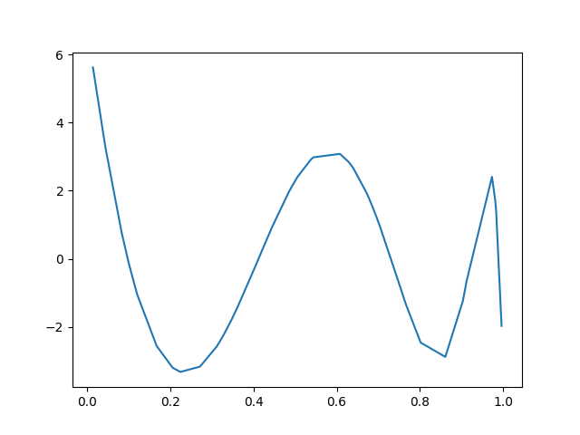
(a)

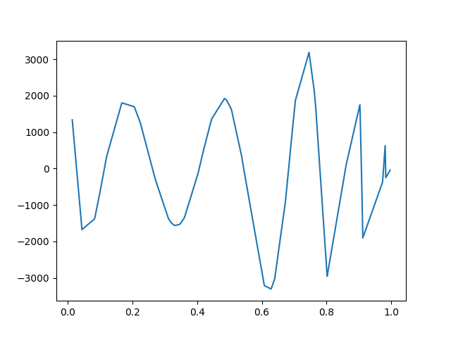
(b)

(c)

(d)

Figure 2: Top row: source condition element $v$ computed for the model $\varphi$ in (17) and $\phi$ in (22) (from left to right, respectively). Note the difference in the y-axis scales: the norm of the source condition for the higher order polynomial is much higher and has larger oscillations than the ones for the lower order model. Bottom row: comparison between $\Phi^{\top}v$ and the sign of the true coefficients $w^{\dagger}$. For both plots, every time $\text{sign}(w^{\dagger})=\pm 1$, then also $\Phi^{\top}v=\pm 1$. This indicates that the estimated source condition $v$ is correct.

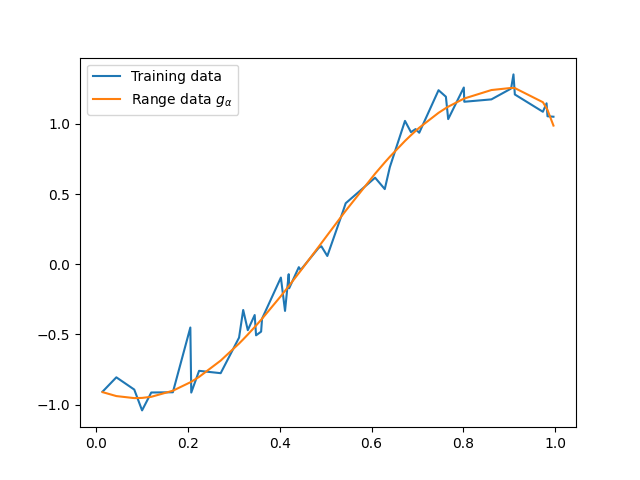
(a)

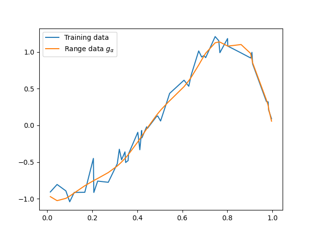
(b)

Figure 3: Comparison between noisy samples $f^{\delta}$ and range condition values $g_{\alpha}$ computed for the model $\varphi$ in (17) and $\phi$ in (22) (from left to right, respectively).

4.2 2D example: Fourier sub-sampling

As a next example, we consider the inverse problem of sub-sampling the Fourier domain of two-dimensional images. If we restrict ourselves to Cartesian grids, we can describe this inverse problem mathematically via the operator equation

$$S\mathcal{F}u^{\dagger}=f\,$$

where $u^{\dagger}\in\mathbb{R}^{n_{y}\times n_{x}}$ denotes the unknown, two-dimensional discrete image, $f\in\mathbb{C}^{m}$ the sub-sampled Fourier data, $\mathcal{F}\colon\mathbb{R}^{n_{y}\times n_{x}}\rightarrow\mathbb{C}^{n_{y}\times n_{x}}$ the two-dimensional discrete Fourier transform, i.e.

$$(\mathcal{F}u)_{pq}=\frac{1}{\sqrt{n_{x}n_{y}}}\sum_{l=0}^{n_{y}-1}\sum_{j=0}^{n_{x}-1}u_{lj}\,e^{-i\frac{2\pi pl}{n_{y}}}e^{-i\frac{2\pi qj}{n_{x}}}\,,$$

for $p\in\{0,\ldots,n_{y}-1\}$ and $q\in\{0,\ldots,n_{x}-1\}$, and $S\colon\mathbb{C}^{n_{y}\times n_{x}}\rightarrow\mathbb{C}^{m}$ the sampling operator that selects samples from the Cartesian grid. Since the operator $\mathcal{F}$ is orthogonal, it holds that $\mathcal{F}^{\top}=\mathcal{F}^{-1}$. For our numerical experiments we choose $J$ to be the (discretised) isotropic total variation, i.e. $J=\text{TV}\colon\mathbb{R}^{n_{y}\times n_{x}}\rightarrow\mathbb{R}$ with

$$\text{TV}(u)=\sum_{i=1}^{n_{y}-1}\sum_{j=1}^{n_{x}-1}\sqrt{\left|u_{(i+1)j}-u_{ij}\right|^{2}+\left|u_{i(j+1)}-u_{ij}\right|^{2}}\,.$$

In order to compute source condition elements $\mathcal{F}^{-1}S^{\top}v\in\partial\text{TV}(u^{\dagger})$, we make use of the range condition reformulation described in Section 3.3 and minimise (15) via explicit coordinate descent as described in (16), which for our problem reads

$$\begin{split}v^{k+1}&=v^{k}-\tau S\mathcal{F}\left(\mathcal{F}^{-1}S^{\top}v^{k}-A^{\top}q^{k}\right)\,,\\ q^{k+1}&=q^{k}-\sigma\left(A\left(A^{\top}q^{k}-\mathcal{F}^{-1}S^{\top}v^{k+1}\right)+\text{prox}_{\|\cdot\|_{2,1}}\left(Au^{\dagger}+q^{k}\right)-Au^{\dagger}\right)\,.\end{split}$$ (23)

Here $A\colon\mathbb{R}^{n_{y}\times n_{x}}\rightarrow\mathbb{R}^{(n_{y}-1)\times(n_{x}-1)\times 2}$ is the (forward) finite-difference discretisation of the gradient, i.e.

$$(Au)_{ijp}=\begin{cases}u_{(i+1)j}-u_{ij}&p=1\\ u_{i(j+1)}-u_{ij}&p=2\end{cases}\,,$$

for $i\in\{1,\ldots,n_{y}-1\}$ and $j\in\{1,\ldots,n_{x}-1\}$, and $\text{prox}_{\|\cdot\|_{2,1}}$ denotes the proximal map with respect to the function $\|\cdot\|_{2,1}\colon\mathbb{R}^{(n_{y}-1)\times(n_{x}-1)\times 2}\rightarrow\mathbb{R}$ defined as

$$\|q\|_{2,1}=\sum_{i=1}^{n_{y}-1}\sum_{j=1}^{n_{x}-1}\sqrt{\left|q_{ij1}\right|^{2}+\left|q_{ij2}\right|^{2}}\,.$$

The proximal map for this functions reads

$$\left(\text{prox}_{\|\cdot\|_{2,1}}(z)\right)_{ijp}=\frac{z_{ijp}}{\sqrt{|z_{ij1}|^{2}+|z_{ij2}|^{2}}}\max\left(\sqrt{|z_{ij1}|^{2}+|z_{ij2}|^{2}}-1,0\right)\,,$$

for $i\in\{1,\ldots,n_{y}-1\}$, $j\in\{1,\ldots,n_{x}-1\}$ and $p\in\{1,2\}$. We choose the positive step-size parameters $\tau=1$ and $\sigma=1/8$, in order to guarantee that (23) converges to a global minimiser of (15) for any initialisation, assuming that one exists. Note that throughout this section, we will always initialise the variables $v^{0}$ and $q^{0}$ with zeros of the correct dimensions.

(a) Shepp-Logan phantom

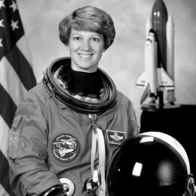
(b) Eileen Collins

Figure 4: Two images that we use for the numerical results presented in this section.

In the following, we show the results for the two choices $u^{\dagger}$ visualised in Figure 4. One image depicts the famous Shepp-Logan phantom, while the other depicts (a grayscale version of) the image of astronaut Eileen Collins.

4.2.1 Shepp-Logan phantom

We begin our discussion of numerical results in this section with the Shepp-Logan phantom. We a use a gray-scale version with $n_{y}=n_{x}=400$ pixels. Before we begin solving the inverse problem of recovering the phantom from low-pass filtered Fourier data, we verify empirically that the Shepp-Logan phantom satisfies the source condition $v\in\partial\text{TV}(u^{\dagger})$, where $u^{\dagger}$ denotes the Shepp-Logan phantom. In order to compute $v$, we evaluate (23) with $S$ being the identity operator, without any Fourier operator and with the parameter choices $\tau=1$ and $\sigma=1/9$ since $\|A\|<8$ ([18]), and stop the iteration once the Euclidean norm of the partial derivatives satisfies $\frac{1}{2}(\|A(A^{\top}q^{K}-v^{K})+\text{prox}_{\|\cdot\|_{2,1}}(Au^{\dagger}+q^{K})-Au^{\dagger}\|+\|v^{K}-A^{\top}q^{K}\|)\leq 3.84\times 10^{-14}$. The corresponding iterates $v^{K}$ and $q^{K}$ are visualised in Figure 5. The Euclidean norm of $v^{K}$ is approximately $\|v^{K}\|\approx 101.78$, which means that we can accurately quantify error estimates of the form (4) for the Shepp-Logan phantom for the inverse problem of denoising.

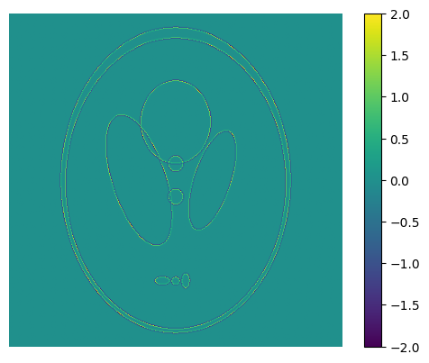
(a) $v^{K}$

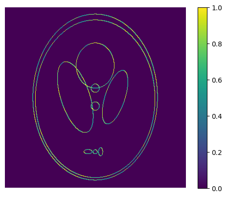
(b) $\sqrt{|q_{1}^{K}|^{2}+|q_{2}^{K}|^{2}}$

Figure 5: Figure 5a depicts the source condition element $v^{K}$ that satisfies $v^{K}\in\partial\text{TV}(u^{\dagger})$ for the Shepp-Logan phantom $u^{\dagger}$. Figure 5b shows the corresponding vector $q^{K}$ such that $A^{\top}q^{K}=v^{K}$. As one would expect from an element in the subgradient, the Euclidean norm of $q^{K}$ with respect to the vector components is bounded by one.

We now want to move on to the inverse problem of estimating the Shepp-Logan phantom from low-pass filtered Fourier data. We choose a square low-pass filter of size $130\times 130$ around the centre frequency. The Fourier transform of the Shepp-Logan phantom and the corresponding low-pass filter are visualised in Figure 6.

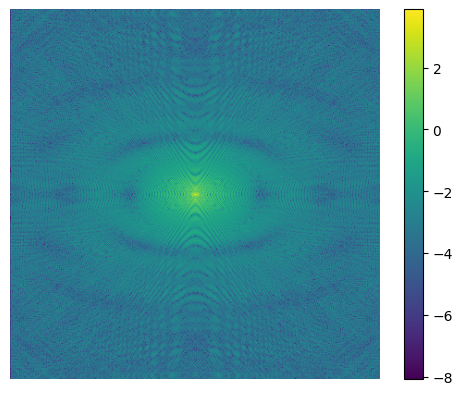
(a) Fourier transformed data

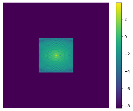
(b) Sub-sampled Fourier transformed data

Figure 6: The Fourier transform of the Shepp-Logan phantom depicted in Figure 4a, and the sub-sampled Fourier transform that emulates a simple low-pass filter. Note that we depict the logarithm of the absolute value of the Fourier transformed data plus the constant $1/4000$ for better visualisation.

We now employ the same algorithmic strategy, namely (23), but where $S$ corresponds to the low-pass sub-sampling. In contrast to the previous example, the decrease of the norm of the partial derivatives is much slower, and we stop the iteration after 1000 iterations, with an approximate value of $0.12$. This indicates that the problem is computationally much harder to solve or that a source condition element does not exist and can therefore not be computed. However, we can certainly use the output $v^{K}$ and $q^{K}$ for $K=1000$ as an approximate source condition element, which we visualise in Figure 7.

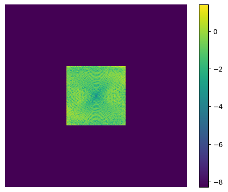
(a) $v^{K}$

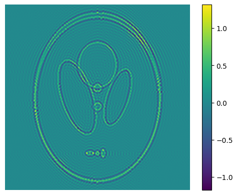
(b) Backprojection $\mathcal{F}^{-1}S^{\top}v^{K}$

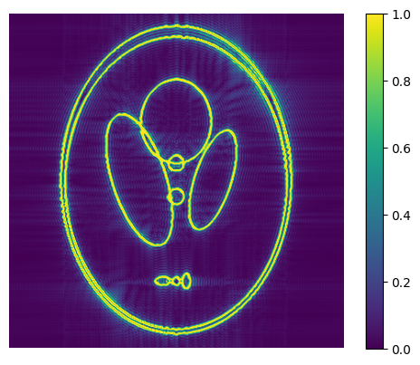
(c) $\sqrt{|q_{1}^{K}|^{2}+|q_{2}^{K}|^{2}}$

Figure 7: The approximate source condition element $v^{K}$ computed with (23) after $K=1000$ iterations (left), the application of $\mathcal{F}^{-1}S^{\top}$ to $v^{K}$ (middle) and the Euclidean vector norm of the vector-field $q^{K}$ of the corresponding subgradient $A^{\top}q^{K}$ (right).

We immediately observe that the scaling of $\mathcal{F}^{-1}S^{\top}v^{K}$ is fairly different from $v^{K}$ in the denoising case, with values mostly in the range of $[-1,1]$ instead of $[-2,2]$. Interestingly, the norm of $v^{K}$ after $K=1000$ iterations for this low-pass filter example is $\|v^{K}\|\approx 72.79$, which is significantly smaller than the $101.78$ that we encountered in the denoising case. The reason for this could be that we did not manage to solve the optimisation problem to the same accuracy (maybe because a source condition element does not exist). Another reason could be that the small $130\times 130$ window of the low-pass filter, which allows $v^{k}$ to only have 16900 instead of 160000 non-zero values, has an impact on the norm of the (approximate) source condition element. The latter also explains the difference in scale of the projection $\mathcal{F}^{-1}S^{\top}v^{K}$ shown in Figure 7b. We also want to emphasise that the Euclidean norm of the vector-field $q^{K}$ is not strictly bounded by one (even though the visualisation in Figure 7c seems to suggest this), but that some values exceed this threshold. This is another indicator that for this example a source condition element is approximated, but not found.

Another indicator that $v^{K}$ is only an approximate source condition element can be found with the help of the relation between source and range condition (RC1). With the range condition we can immediately characterise data $g_{\alpha}=\alpha v+Ku^{\dagger}$ given a source condition element $v$, or $g_{\alpha}^{K}=\alpha v^{K}+S\mathcal{F}u^{\dagger}$ for our example. We set $\alpha$ to the arbitrary value of $\alpha=1/2$ and compute a solution of (3) from the data $g_{\alpha}^{K}$ with an implementation of the primal-dual hybrid gradient (PDHG) method [19]. We choose the PDHG version described in [5] with step-sizes $\tau=1/8$ and $\sigma=1$, and iterate for $N=1000$ iterations until the iterates of the primal ($u^{N}$) and dual variable ($q^{N}$) of the PDHG method satisfy $1/2*(\|u^{N}-u^{N-1}\|/\|u^{N}\|+\|q^{N}-q^{N-1}\|/\|q^{K}\|)<6.85\times 10^{-5}$. The results together with the data $g_{\alpha}$ are visualised in Figure 8.

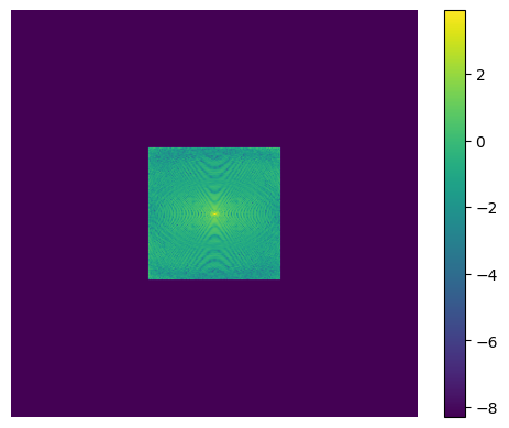
(a) Range condition data $g_{\alpha}^{K}$

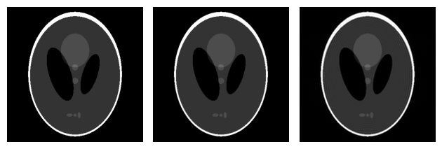
(b) Sanity check

(c) Sanity check close-up

Figure 8: This figure shows the (approximate) range condition data $g_{\alpha}^{K}=\alpha v^{K}+S\mathcal{F}u^{\dagger}$ for $\alpha=1/2$ in Figure 8a. In Figure 8b we see the original Shepp-Logan phantom $u^{\dagger}$ (left), the approximate solution $u^{N}$ of (3) computed with the PDHG method for $\alpha=1/2$ and input data $g_{\alpha}^{K}$ (middle) and the linear low-pass filtered reconstruction $\mathcal{F}^{-1}S^{\top}S\mathcal{F}u^{\dagger}$ (right), and a close-up of the three small-scale features at the bottom of the phantom for $u^{\dagger}$ (left), $u^{N}$ (middle) and $\mathcal{F}^{-1}S^{\top}S\mathcal{F}u^{\dagger}$ (right) in Figure 8c.

We see from the close-up in Figure 8c that the reconstruction does not exactly match the Shepp-Logan phantom, which is what we would expect if $v^{K}$ was a source condition element. Hence, these results are another indicator that we either terminated the iteration too soon or that a source condition element does not exist. However, we nevertheless observe that the reconstruction $u^{N}$ for data $g_{\alpha}^{K}$ is a good approximation of the Shepp-Logan phantom and reasonably better than the traditional low-pass filter as one would expect. Another interesting observation is that if we were to define $u^{\dagger}=u^{N}$, we can guarantee that $u^{\dagger}$ satisfies the source condition with source condition element $v$ that satisfies $\|v\|\approx 72.79$. This is lower than the value of $101.78$ that we obtained in the denoising case for the Shepp-Logan phantom, and likely a result of this new $u^{\dagger}$ being smoother than the Shepp-Logan phantom. However, the nature of the inverse problem with the low-pass filter forward operator might also play a role for the lower value of the norm as it seems plausible that for this type of filter errors are amplified less strongly, since the transpose operation $\mathcal{F}^{-1}S^{\top}$ filters high-frequency errors quite effectively.

We are going to see in Section 4.3 that we can find a more data-adaptive sampling strategy (compared to the low-pass filter) for which we can recover $u_{\alpha}\in\mathcal{R}_{\alpha}(g_{\alpha})$ almost perfectly from even fewer samples.

4.2.2 Eileen Collins

We perform identical experiments as in the previous section, but this time we choose an element $u^{\dagger}$ for which satisfying the source condition is highly unlikely: an image with textures and fine-scale details. We pick the astronaut image of Eileen Collings depicted in Figure 4b. We use a gray-scale version that is down-scaled to $n_{y}=400$ and $n_{x}=400$ pixels as our image $u^{\dagger}$, and we try to empirically verify if the astronaut image satisfies a source condition of the form $\mathcal{F}^{-1}S^{\top}v\in\partial\text{TV}(u^{\dagger})$.

Similar to the previous example, we choose a square low-pass filter, but this time of size $200\times 200$ around the centre frequency. The Fourier transform of the Eileen Collins image and the corresponding low-pass filter are visualised in Figure 9a and Figure 9b, respectively.

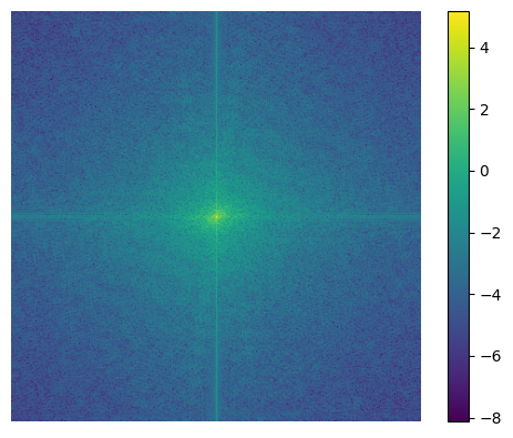
(a) Fourier transformed data

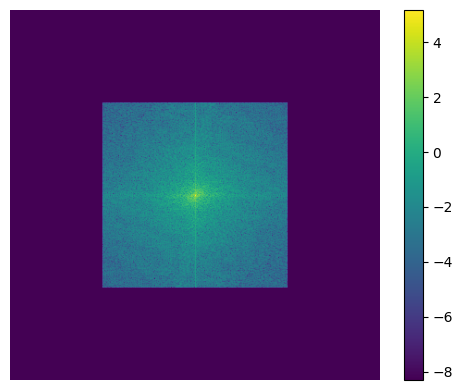
(b) Sub-sampled Fourier transformed data

Figure 9: The Fourier transform of the astronaut image depicted in Figure 4b, and the sub-sampled Fourier transform that emulates a simple low-pass filter. Note that we depict the logarithm of the absolute value of the Fourier transformed data plus the constant $1/4000$ for better visualisation.

In analogy to the previous section, we evaluate (23) with the parameter choices $\tau=1$ and $\sigma=1/8$, initialise with zero arrays and stop the iteration after $K=1000$ iterations when the Euclidean norm of the partial derivatives satisfies $\frac{1}{2}(\|A(A^{\top}q^{K}-\mathcal{F}^{-1}S^{\top}v^{K}+\text{prox}_{\|\cdot\|_{2,1}}(Au^{\dagger}+q^{K})-Au^{\dagger}\|+\|\mathcal{F}^{-1}S^{\top}v^{K}-A^{\top}q^{K}\|)\leq 0.59$. The corresponding iterates $v^{K}$ and $q^{K}$ are visualised in Figure 10a and Figure 10c, respectively. The Euclidean norm of $v^{K}$ is approximately $\|v^{K}\|\approx 255.15$, but we have to keep in mind that the source condition element is likely only an approximate source condition element, given the nature of the signal $u^{\dagger}$ and the value of the norm of the partial derivatives that is still very high after $K=1000$ iterations. Nevertheless, the value $\|v^{K}\|$ is much larger compared to the Shepp-Logan example, which is what we would expect from a textured image $u^{\dagger}$ with fine details.

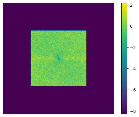
(a) $v^{K}$

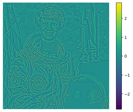
(b) Backprojection $\mathcal{F}^{-1}S^{\top}v^{K}$

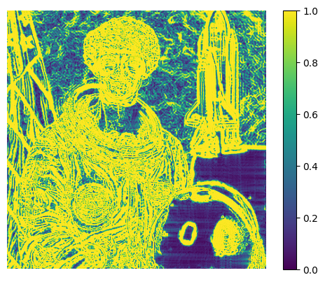
(c) $\sqrt{|q_{1}^{K}|^{2}+|q_{2}^{K}|^{2}}$

Figure 10: The approximate source condition element $v^{K}$ computed with (23) after $K=1000$ iterations (left), the application of $\mathcal{F}^{-1}S^{\top}$ to $v^{K}$ (middle) and the Euclidean vector norm of the vector-field $q^{K}$ of the corresponding subgradient $A^{\top}q^{K}$ (right).

We want to emphasise that the Euclidean norm of the vector-field $q^{K}$ is not strictly bounded by one (even though the visualisation in Figure 10c seems to suggest this), but that some values exceed this threshold, which is another indicator that for this example a source condition element is only approximated, but not found.

Similarly to the Shepp-Logan phantom, we check (approximate) solutions of (3) for the range data $g_{\alpha}=\alpha v+S\mathcal{F}u^{\dagger}$ for $\alpha=1/2$. For our example, we define $g_{\alpha}^{K}=\alpha v^{K}+S\mathcal{F}u^{\dagger}$ and compute a solution of (3) with the PDHG method as described in the previous section (for identical initialisation and parameter choices). After $N=1000$ iterations we compute primal ($u^{N}$) and dual ($q^{N}$) iterates that satisfy $(\|u^{N}-u^{N-1}\|/\|u^{N}\|+\|q^{N}-q^{N-1}\|/\|q^{N}\|)/2<9.29\times 10^{-5}$. The result $u^{N}$ together with the data $g_{\alpha}^{N}$ are visualised in Figure 11.

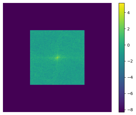
(a) Range condition data $g_{\alpha}^{K}$

(b) Sanity check

(c) Sanity check close-up

Figure 11: This figure shows the (approximate) range condition data $g_{\alpha}^{K}=\alpha v^{K}+S\mathcal{F}u^{\dagger}$ for $\alpha=1/2$ in Figure 11a. In Figure 11b we see the image $u^{\dagger}$ of Eileen Collings (left), the approximate solution $u^{N}$ of (3) computed with the PDHG method for $\alpha=1/2$ and input data $g_{\alpha}^{K}$ (middle) and the linear low-pass filtered reconstruction $\mathcal{F}^{-1}S^{\top}S\mathcal{F}u^{\dagger}$ (right), and a close-up of some facial small-scale features of $u^{\dagger}$ (left), $u^{N}$ (middle) and $\mathcal{F}^{-1}S^{\top}S\mathcal{F}u^{\dagger}$ (right) in Figure 11c.

We clearly see that the reconstruction $u^{N}$ is not identical to $u^{\dagger}$ but rather a cartoon-like approximation that misses high-scale features such as textures. This does not come as a surprise as we would expect this from a total-variation approximation that does not have access to the high-scale features that the low-pass filter suppresses. We are going to see in Section 4.3 that we can improve the reconstruction by identifying a more adaptive sampling pattern when estimating the approximate source condition element.

4.3 Optimal sampling in the Fourier domain

In Section 4.2 we studied the empirical computation of source condition and approximate source condition elements for the variational regularisation of the form

$$u_{\alpha}\in\operatorname*{\arg\min}_{u\in\mathbb{R}^{n_{y}\times n_{x}}}\left\{\frac{1}{2}\left\|S\mathcal{F}u-f^{\delta}\right\|^{2}+\alpha\text{TV}(u)\right\}\,.$$

In this section we want to take a step further and also estimate the sampling pattern that defines the sampling operator $S$. This idea is not new and has applications, for example, in magnetic resonance imaging (cf. [49]). However, in this section we present a much simpler approach for estimating $S$ compared to works such as [49]. Most importantly, the approach can be phrased as a convex optimisation problem depending on how we choose to enforce sparsity of $\tilde{v}$, while most alternative approaches constitute non-convex optimisation problems.

The approach is summarised as follows. We assume that $S$ no longer maps onto $\mathbb{C}^{m}$, but that $S$ maps onto $\mathbb{C}^{n_{y}\times n_{x}}$ and that it is a diagonal operator with zero-entries on the diagonal wherever the sampling mask is zero. If we consider the standard source condition $\mathcal{F}^{-1}S^{\top}v\in\partial\text{TV}(u^{\dagger})$ for the above problem, we can define $\tilde{v}\colon=S^{\top}v\in\mathbb{C}^{n_{y}\times n_{x}}$, and estimate $\tilde{v}$ instead of $v$. Since $\tilde{v}$ has to be sparse by nature in order to emulate sub-sampling, we can estimate $\tilde{v}$ by solving

$$\min_{\tilde{v},q^{\dagger}}\frac{1}{2}\|\mathcal{F}^{-1}\tilde{v}-A^{\top}q^{\dagger}\|^{2}+G_{\|\cdot\|_{2,1}}(q^{\dagger})+\beta J(\tilde{v})\,,$$ (24)

where $J$ is a sparsity-inducing regularisation function, e.g. $J(\tilde{v})=\|\tilde{v}\|_{1}=\sum_{i=1}^{n_{y}}\sum_{j=1}^{n_{x}}|\tilde{v}_{ij}|$ where $|\cdot|$ denotes the complex modulus, and $\beta>0$ is a penalisation parameter that controls the level of sparsity of $\tilde{v}$. We then minimise (24) via the proximal alternating linearised minimisation (PALM) algorithm [56, 6], i.e. we approximate a solution of (24) by iterating

$$\begin{split}\tilde{v}^{k+1}&=\text{prox}_{\beta J}\left(\tilde{v}^{k}-\tau\left(\tilde{v}^{k}-\mathcal{F}A^{\top}q^{k}\right)\right)\,,\\ q^{k+1}&=q^{k}-\sigma\left(A\left(A^{\top}q^{k}-\mathcal{F}^{-1}\tilde{v}^{k+1}\right)+\text{prox}_{\|\cdot\|_{2,1}}\left(q^{k}+Au^{\dagger}\right)-Au^{\dagger}\right)\,,\end{split}$$ (25)

for $k\in\mathbb{N}$, initial values $\tilde{v}^{0}$ and $q^{0}$ and suitable step-size parameters $\tau$ and $\sigma$.

In the following, we approximate $\tilde{v}^{K}$ and $q^{K}$ for the arbitrary choice $K=1000$. We then estimate the mask that determines the zero and non-zero entries on the diagonal of $S$ by simply identifying the zero and non-zero entries of $\tilde{v}$. Please note that we manually enforce that the lowest frequency is included in the mask, as it otherwise would be excluded since total variation subgradients have zero mean. Subsequently, we estimate $v$ by solving (23) with the estimated sub-sampling operator $S$ from the previous step, for $K=1000$ iterations. We have conducted experiments for the same examples visualised in Figure 4, which are described in the next two sections.

4.3.1 Shepp-Logan phantom

We begin with the Shepp-Logan phantom as seen in Figure 4a and compute the corresponding element $\tilde{v}^{K}$ via (25) with zero-initialisation, $J=\beta\|\cdot\|_{1}$ and the parameter $\beta=0.1$. The corresponding $\tilde{v}^{K}$, the mask of all non-zero coefficients and the mask of the 16900 largest Fourier coefficients (in magnitude) are visualised in Figure 12. Please note that for $\beta=0.1$ the number of non-zero coefficients of $\tilde{v}^{K}$ after $K=1000$ iterations is 14553, which is comparable but even slightly lower than the 16900 non-zero coefficients that were used in the low-pass filter example in Section 4.2.1.

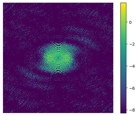
(a) $\tilde{v}^{K}$

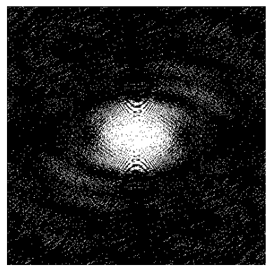
(b) Sampling pattern

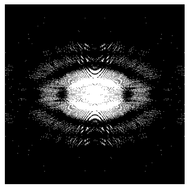
(c) Largest Fourier coefficients

Figure 12: Figure 12a shows the (approximate) source condition element for the Shepp-Logan phantom computed with (25). Figure 12b shows the corresponding mask of all 14553 non-zero (white) versus 145447 zero (black) coefficients. For comparison, Figure 12c shows the mask of the 16900 Fourier coefficients with largest magnitude (white) versus the 143100 Fourier coefficients with smallest magnitude (black).

We want to emphasise that the learned mask differs substantially from the mask that stems from the largest Fourier coefficients (in magnitude). In particular, low-frequency information is traded in for high-frequency information since the total variation regularisation is very effective at establishing information from limited low-frequency data but very ineffective at generating high-frequency information.

Next, given the mask we estimate $v$ via (23) and obtain $v^{K}$ for $K=1000$. Note that the corresponding norm is $\|v^{K}\|\approx 113.93$, which is slightly larger but fairly comparable to the norm that we established in the denoising setting. Subsequently, we perform another sanity-check and compute an approximation of (3) for data $g_{\alpha}^{K}=\alpha v^{K}+S\mathcal{F}u^{\dagger}$ for $\alpha=1/2$ via the PDHG method with the same initialisation and parameter configurations as described in Section 4.2.1 and visualise the results in Figure 13.

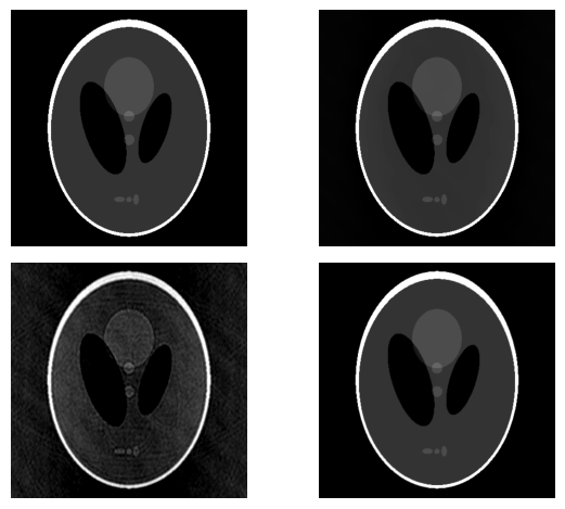
(a) Reconstructions

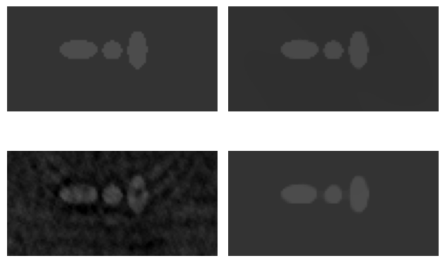
(b) Close-up

Figure 13: Figure 13a shows the Shepp-Logan phantom (top-left), the approximation $u^{N}$ of (3) with the learned mask and corresponding range data (top-right), the projection $\mathcal{F}^{-1}S^{\top}S\mathcal{F}u^{\dagger}$ (bottom left) and the approximation $u^{N}$ of (3) with the low-pass filter from Section 4.2.1 (bottom-right). Figure 13b shows a corresponding close-up of the small-scale features at the bottom of the phantom.

In comparison to Section 4.2.1, we observe that we recover the Shepp-Logan phantom almost perfectly whilst using a sampling operator that samples fewer samples than the low-pass sampling operator.

4.3.2 Eileen Collins

We now proceed to the image of Eileen Collins as depicted in Figure 4b and perform the same set of tasks as described in the previous section, i.e. we compute the element $\tilde{v}^{K}$ via (25) with zero-initialisation and for $J=\beta\|\cdot\|_{1}$ for which we choose $\beta=0.24$ this time. The corresponding $\tilde{v}^{K}$, the mask of all non-zero coefficients and the mask of the 40000 largest Fourier coefficients (in magnitude) are visualised in Figure 14. Please note that for $\beta=0.24$ the number of non-zero coefficients of $\tilde{v}^{K}$ after $K=1000$ iterations is 38262, which is comparable but even slightly lower than the 40000 non-zero coefficients that were used in the low-pass filter example in Section 4.2.2.

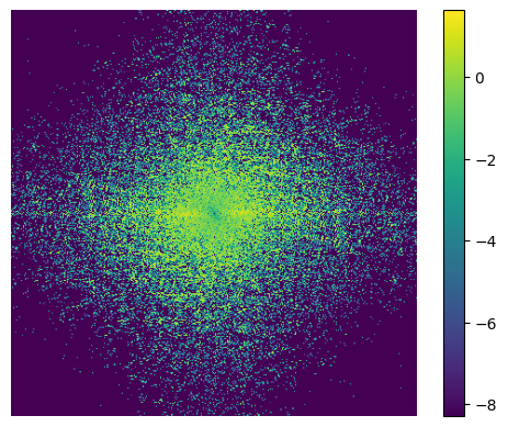
(a) $\tilde{v}^{K}$

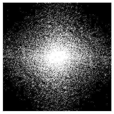
(b) Sampling pattern

(c) Largest Fourier coefficients

Figure 14: Figure 14a shows the (approximate) source condition element for the Eileen Collins image computed with (25). Figure 14b shows the corresponding mask of all 38262 non-zero (white) versus 121738 zero (black) coefficients. For comparison, Figure 14c shows the mask of the 40000 Fourier coefficients with largest magnitude (white) versus the 120000 Fourier coefficients with smallest magnitude (black).

We see that the learned mask differs from that obtained from the Fourier coefficients with largest magnitude. In particular, the information that corresponds to coarse edges in the image $u^{\dagger}$ is less important for the total variation-based model, since it can interpolate this type of missing information rather well. Instead, more higher frequencies corresponding to texture information are being sampled as it is impossible for a total variation-based model to generate textures.

Given the mask, we estimate $v$ via (23) and obtain $v^{K}$ for $K=1000$. Note that the corresponding norm is $\|v^{K}\|\approx 302.47$, which is larger than the norm that we established in the low-pass filter setting. Subsequently, we perform another sanity-check and compute an approximation of (3) for data $g_{\alpha}^{K}=\alpha v^{K}+S\mathcal{F}u^{\dagger}$ for $\alpha=1/2$ via the PDHG method with the same initialisation and parameter configurations as described in Section 4.2.2 and visualise the results in Figure 15.

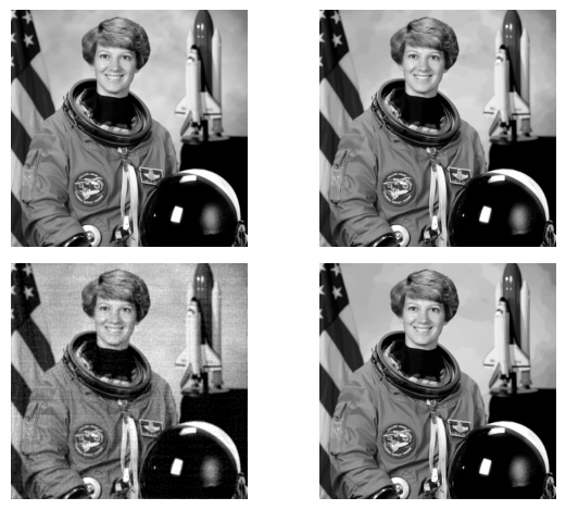
(a) Reconstructions

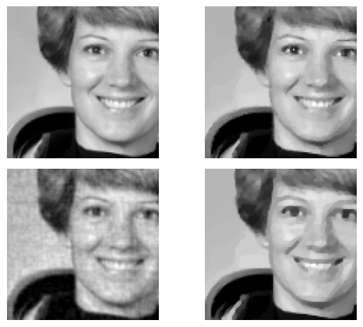
(b) Close-up

Figure 15: Figure 15a shows the image of Eileen Collins (top-left), the approximation $u^{N}$ of (3) with the learned mask and corresponding range data (top-right), the projection $\mathcal{F}^{-1}S^{\top}S\mathcal{F}u^{\dagger}$ (bottom left) and the approximation $u^{N}$ of (3) with the low-pass filter from Section 4.2.2 (bottom-right). Figure 15b shows a corresponding close-up of some of the facial features.

In comparison to Section 4.2.2, we observe that we still have not found been able to verify existence of a source condition element, which is not surprising. We do observe, however, that the recovery of (3) with the range data for the learned sampling operator is much better compared to the recovery with the low-pass sampling operator. We observe several high-frequency features such as the specular highlights in the eyes that are not present in the low-pass filter reconstruction. Please not that the reconstruction with the learned sampling operator uses even fewer samples than the reconstruction with the low-pass sampling operator.

5 Conclusions & Outlook

We conclude this work with a brief summary of its main findings, and provide an outlook of research topics that we have not been able to address but that make for interesting future research.

5.1 Conclusions

In this paper, we have pursued the challenging task of estimating source condition elements as tools for the quantitative analysis of variational regularisation of linear inverse problems. Specifically,

• we considered a rather general Banach space setup, which encompasses a large class of regularisation methods of interest in applications;

• we reformulated the source conditions (and the closely related range conditions) as the solution of convex minimisation problems by means of tools from convex analysis;

• we provided iterative algorithms for the numerical approximation of source (and range) condition elements, which pave the way to quantitative error estimates;

• to demonstrate the performance of the proposed approach, we enclosed a significant set of numerical experiments for processing both 1D and 2D signals;

• we described how the introduced framework can provide insightful inspiration for novel approaches in optimal measurement design: in particular, the proposed procedure of optimal subsampling in the Fourier domain provided promising results.

5.2 Outlook

There are numerous research aspects that we have either addressed only briefly or have not addressed at all. One obvious aspect is that source and range conditions are not only relevant for convergence rates for variational regularisations but other regularisations such as iterative regularisations, too (cf. [16, 4]). Hence, in order to quantify error estimates for such regularisations, identical strategies as proposed in this paper can be deployed. The same also holds true for regularisation methods that are based on more general data fidelity terms as described in (2), for which error estimates also rely on source or range conditions [2].

Further, we did not look into stronger source conditions or variational source conditions as outlined in the introduction, but it should be straight forward to design convex minimisation problems similar to the ones presented in this work for the computation of, e.g., strong source condition elements. We also maintained focus solely on linear inverse problems, while source conditions play a pivotal role for convergence rates of nonlinear inverse problems, too.

Another interesting direction for research is the computation of generalised eigenfunctions or singular vectors as addressed in the introduction. Suppose we are given a function $f$ and we would like to find a function $u_{\lambda}$ that satisfies $\lambda u_{\lambda}\in J(u_{\lambda})$ such that it is close to $f$, then we can formulate the constrained minimisation problem

$$\min_{u}\ B_{J}(u,(1+\lambda)u)\qquad\text{subject to}\qquad\|u-f\|\leq\delta\,,$$

for hyperparameters $\lambda>0$ and $\delta\geq 0$. If a solution $u_{\lambda}$ satisfies $B_{J}(u_{\lambda},(1+\lambda)u_{\lambda})=0$, we can conclude that it is a generalised eigenfunction with eigenvalue $\lambda$ and closest to $f$ within the ball of radius $\delta$.

Last but not least, we want to emphasise that extensions of the proposed minimisation problems can find applications in a wide range of data-driven inverse problems applications such as operator correction and learning data-driven regularisation functionals that we want to briefly describe in the following two sections.

5.2.1 Operator correction

In analogy to the optimal sampling example presented in Section 4.3, one can modify the proposed approaches to perform more general operator corrections beyond sampling. Taking the polynomial regression problem from Section 4.1 as an example, one can consider the following extension of the classical LASSO approach:

$$u_{\alpha}\in\operatorname*{\arg\min}_{u\in\ell^{2}\cap\ell^{1}}\left\{\frac{1}{2}\left\|A\left(Ku-f^{\delta}\right)\right\|^{2}+\alpha\|u\|_{1}\right\}\,.$$

In this example, the goal is to estimate not only the source condition element $v$, but to also estimate a pre-conditioner matrix $A$. We could do so by formulating the non-convex optimisation problem

$$\min_{A,\{v_{i}\}_{i=1}^{s}}\left[\sum_{i=1}^{s}B_{\|\cdot\|_{1}}\left(u_{i}^{\dagger},u_{i}^{\dagger}+K^{\top}A^{\top}v_{i}\right)+\chi_{\|\cdot\|\leq\beta}(v_{i})\right]\,,$$

where we minimise an empirical risk for $s$ vectors of polynomial coefficients $\{u^{\dagger}_{i}\}_{i=1}^{s}$ subject to the constraint that the norm of the source condition elements $v_{i}$ should not exceed the threshold $\beta>0$. If the data is representative, minimising this empirical risk can help preconditioning the forward model and the data to lower the norms of the corresponding source condition elements, which in return ensures better convergence rates of the solution of $u_{\alpha}$ towards true coefficients $u^{\dagger}$.

5.2.2 Construction of data-driven regularisations

One can extend the findings from Section 3 to design data-driven variational regularisation operators $R_{\alpha}$ with convergence rate $\mathcal{O}(\delta)$ and favourable error amplification constant $\|v\|$ in the error estimate (4). In order to do so, we can make the assumption that we have a parametrised variational regularisation operator $R_{\alpha}$ of the form (3) with a regularisation function of the form $J(u)=H(Au+b)$. We can then aim at estimating the linear operator $A$ and the function $b$ by minimising an empirical risk of the form

$$\frac{1}{s}\sum_{i=1}^{s}\left[\Phi(v_{i})+\frac{1}{2}\|K^{\ast}v_{i}-A^{\ast}q^{\dagger}_{i}\|^{2}+B_{H}\left(Au^{\dagger}_{i}+b,q^{\dagger}_{i}+Au^{\dagger}_{i}+b\right)\right]\,,$$

for some suitable regularisation function $\Phi$. In order to keep the error amplification constants $\|v_{i}\|$ bounded, one intuitive choice for $\Phi$ is

$$\Phi(v)=\chi_{\|\cdot\|\leq\beta}(v)\colon=\begin{cases}0&\|v\|\leq\beta\\ \infty&\|v\|>\beta\end{cases}\,,$$

for a positive constant $\beta>0$, similar to the operator correction example in Section 5.2.1. Then one can formulate the constrained, non-convex minimisation problem

$$\min_{\{v_{i}\}_{i=1}^{s},\{q^{\dagger}_{i}\}_{i=1}^{s},A,b}\sum_{i=1}^{s}\left[\chi_{\|\cdot\|\leq\alpha}(v_{i})+\frac{1}{2}\|K^{\ast}v_{i}-A^{\ast}q^{\dagger}_{i}\|^{2}+B_{H}\left(Au^{\dagger}_{i}+b,q^{\dagger}_{i}+Au^{\dagger}_{i}+b\right)\right]\,.$$

Similar to the idea proposed in Section 5.2.1, minimising such an empirical risk can help identifying a suitable operator $A$ (and shift $b$) to lower the norms of the corresponding source condition elements, which in return ensures better convergence rates of the solution of the variational regularisation method towards the solution $u^{\dagger}$ of the inverse problem (1).

Data Availability Statement

The Python codes for this paper will be made available once the revision process is complete.

References

- [1] Amir Beck and Luba Tetruashvili, On the convergence of block coordinate descent type methods, SIAM journal on Optimization 23 (2013), no. 4, 2037–2060.
- [2] Martin Benning and Martin Burger, Error estimates for general fidelities, Electronic Transactions on Numerical Analysis 38 (2011), no. 44-68, 77.
- [3] , Ground states and singular vectors of convex variational regularization methods, Methods and Applications of Analysis 20 (2013), no. 4, 295–334.
- [4] , Modern regularization methods for inverse problems, Acta Numerica 27 (2018), 1–111.
- [5] Martin Benning and Erlend Skaldehaug Riis, Bregman methods for large-scale optimisation with applications in imaging, Handbook of Mathematical Models and Algorithms in Computer Vision and Imaging: Mathematical Imaging and Vision (2021), 1–42.
- [6] Jérôme Bolte, Shoham Sabach, and Marc Teboulle, Proximal alternating linearized minimization for nonconvex and nonsmooth problems, Mathematical Programming 146 (2014), no. 1, 459–494.
- [7] Farid Bozorgnia, Leon Bungert, and Daniel Tenbrinck, The infinity laplacian eigenvalue problem: reformulation and a numerical scheme, arXiv preprint arXiv:2004.08127 (2020).
- [8] Lev M Bregman, The relaxation method of finding the common point of convex sets and its application to the solution of problems in convex programming, USSR computational mathematics and mathematical physics 7 (1967), no. 3, 200–217.
- [9] Tatiana A Bubba, Martin Burger, Tapio Helin, and Luca Ratti, Convex regularization in statistical inverse learning problems, arXiv preprint arXiv:2102.09526 (2021).
- [10] Tatiana A Bubba and Luca Ratti, Shearlet-based regularization in statistical inverse learning with an application to x-ray tomography, Inverse Problems 38 (2022), no. 5, 054001.
- [11] Leon Bungert, Ester Hait-Fraenkel, Nicolas Papadakis, and Guy Gilboa, Nonlinear power method for computing eigenvectors of proximal operators and neural networks, SIAM Journal on Imaging Sciences 14 (2021), no. 3, 1114–1148.
- [12] Martin Burger, Lina Eckardt, Guy Gilboa, and Michael Moeller, Spectral representations of one-homogeneous functionals, Scale Space and Variational Methods in Computer Vision: 5th International Conference, SSVM 2015, Lège-Cap Ferret, France, May 31-June 4, 2015, Proceedings, Springer, 2015, pp. 16–27.
- [13] Martin Burger, Guy Gilboa, Michael Moeller, Lina Eckardt, and Daniel Cremers, Spectral decompositions using one-homogeneous functionals, SIAM Journal on Imaging Sciences 9 (2016), no. 3, 1374–1408.
- [14] Martin Burger, Tapio Helin, and Hanne Kekkonen, Large noise in variational regularization, Transactions of Mathematics and its Applications 2 (2018), no. 1, tny002.
- [15] Martin Burger and Stanley Osher, Convergence rates of convex variational regularization, Inverse problems 20 (2004), no. 5, 1411.
- [16] Martin Burger, Elena Resmerita, and Lin He, Error estimation for Bregman iterations and inverse scale space methods in image restoration, Computing 81 (2007), no. 2, 109–135.
- [17] Emmanuel J Candès, Justin Romberg, and Terence Tao, Robust uncertainty principles: Exact signal reconstruction from highly incomplete frequency information, IEEE Transactions on information theory 52 (2006), no. 2, 489–509.
- [18] Antonin Chambolle, An algorithm for total variation minimization and applications, Journal of Mathematical imaging and vision 20 (2004), 89–97.
- [19] Antonin Chambolle and Thomas Pock, An introduction to continuous optimization for imaging, Acta Numerica 25 (2016), 161–319.
- [20] Guy Chavent and Karl Kunisch, Regularization of linear least squares problems by total bounded variation, ESAIM: Control, Optimisation and Calculus of Variations 2 (1997), 359–376.
- [21] Ingrid Daubechies, Michel Defrise, and Christine De Mol, An iterative thresholding algorithm for linear inverse problems with a sparsity constraint, Communications on Pure and Applied Mathematics: A Journal Issued by the Courant Institute of Mathematical Sciences 57 (2004), no. 11, 1413–1457.
- [22] David L Donoho, Superresolution via sparsity constraints, SIAM Journal on mathematical analysis 23 (1992), no. 5, 1309–1331.
- [23] Heinz W Engl, Karl Kunisch, and Andreas Neubauer, Convergence rates for Tikhonov regularisation of non-linear ill-posed problems, Inverse Problems 5 (1989), no. 4, 523.
- [24] Heinz Werner Engl, Martin Hanke, and Andreas Neubauer, Regularization of inverse problems, vol. 375, Springer Science & Business Media, 1996.
- [25] Jens Flemming, Generalized Tikhonov regularization and modern convergence rate theory in Banach spaces, Shaker-Verlag, 2012.
- [26] Guy Gilboa, Nonlinear band-pass filtering using the tv transform, 2014 22nd European Signal Processing Conference (EUSIPCO), IEEE, 2014, pp. 1696–1700.
- [27] , A total variation spectral framework for scale and texture analysis, SIAM journal on Imaging Sciences 7 (2014), no. 4, 1937–1961.
- [28] , Nonlinear eigenproblems in image processing and computer vision, Springer, 2018.
- [29] Guy Gilboa, Michael Moeller, and Martin Burger, Nonlinear spectral analysis via one-homogeneous functionals: overview and future prospects, Journal of Mathematical Imaging and Vision 56 (2016), 300–319.
- [30] Markus Grasmair, Markus Haltmeier, and Otmar Scherzer, Sparse regularization with penalty term, Inverse Problems 24 (2008), no. 5, 055020.
- [31] Markus Grasmair, Otmar Scherzer, and Markus Haltmeier, Necessary and sufficient conditions for linear convergence of -regularization, Communications on Pure and Applied Mathematics 64 (2011), no. 2, 161–182.
- [32] Torsten Hein and Bernd Hofmann, Approximate source conditions for nonlinear ill-posed problems—chances and limitations, Inverse Problems 25 (2009), no. 3, 035003.
- [33] Jean-Baptiste Hiriart-Urruty and Claude Lemaréchal, Fundamentals of convex analysis, Springer Science & Business Media, 2004.
- [34] Bernd Hofmann, D Düvelmeyer, and Klaus Krumbiegel, Approximate source conditions in Tikhonov regularization-new analytical results and some numerical studies, Mathematical Modelling and Analysis 11 (2006), no. 1, 41–56.
- [35] Bernd Hofmann, Barbara Kaltenbacher, Christiane Pöschl, and Otmar Scherzer, A convergence rates result for Tikhonov regularization in Banach spaces with non-smooth operators, Inverse Problems 23 (2007), no. 3, 987.
- [36] Thorsten Hohage and Philip Miller, Optimal convergence rates for sparsity promoting wavelet-regularization in Besov spaces, Inverse Problems 35 (2019), no. 6, 065005.
- [37] Thorsten Hohage and Frederic Weidling, Characterizations of variational source conditions, converse results, and maxisets of spectral regularization methods, SIAM Journal on Numerical Analysis 55 (2017), no. 2, 598–620.
- [38] Pierre-Louis Lions and Bertrand Mercier, Splitting algorithms for the sum of two nonlinear operators, SIAM Journal on Numerical Analysis 16 (1979), no. 6, 964–979.
- [39] Subhadip Mukherjee, Carola-Bibiane Schönlieb, and Martin Burger, Learning convex regularizers satisfying the variational source condition for inverse problems, NeurIPS 2021 Workshop on Deep Learning and Inverse Problems.
- [40] David Bryant Mumford and Jayant Shah, Optimal approximations by piecewise smooth functions and associated variational problems, Communications on pure and applied mathematics (1989).
- [41] Yurii Nesterov, A method for unconstrained convex minimization problem with the rate of convergence o (1/k^ 2), Doklady an ussr, vol. 269, 1983, pp. 543–547.
- [42] Raz Z Nossek and Guy Gilboa, Flows generating nonlinear eigenfunctions, Journal of Scientific Computing 75 (2018), 859–888.
- [43] Ronny Ramlau and Elena Resmerita, Convergence rates for regularization with sparsity constraints, Electron. Trans. Numer. Anal 37 (2010), 87–104.
- [44] Elena Resmerita, Regularization of ill-posed problems in Banach spaces: convergence rates, Inverse Problems 21 (2005), no. 4, 1303.
- [45] Leonid I Rudin, Stanley Osher, and Emad Fatemi, Nonlinear total variation based noise removal algorithms, Physica D: nonlinear phenomena 60 (1992), no. 1-4, 259–268.
- [46] Otmar Scherzer, Markus Grasmair, Harald Grossauer, Markus Haltmeier, and Frank Lenzen, Variational methods in imaging, (2009).
- [47] Marie Foged Schmidt, Martin Benning, and Carola-Bibiane Schönlieb, Inverse scale space decomposition, Inverse Problems 34 (2018), no. 4, 045008.
- [48] Thomas Schuster, Barbara Kaltenbacher, Bernd Hofmann, and Kamil S Kazimierski, Regularization methods in Banach spaces, vol. 10, Walter de Gruyter, 2012.
- [49] Ferdia Sherry, Martin Benning, Juan Carlos De los Reyes, Martin J Graves, Georg Maierhofer, Guy Williams, Carola-Bibiane Schönlieb, and Matthias J Ehrhardt, Learning the sampling pattern for mri, IEEE Transactions on Medical Imaging 39 (2020), no. 12, 4310–4321.
- [50] Ulrich Tautenhahn, Optimality for ill-posed problems under general source conditions, Numerical Functional Analysis and Optimization 19 (1998), no. 3-4, 377–398.
- [51] Robert Tibshirani, Regression shrinkage and selection via the lasso, Journal of the Royal Statistical Society: Series B (Methodological) 58 (1996), no. 1, 267–288.
- [52] Andrey N. Tikhonov, On the stability of inverse problems, Dokl. Akad. Nauk SSSR, vol. 39, 1943, pp. 195–198.
- [53] , Solution of incorrectly formulated problems and the regularization method, Soviet Math. 4 (1963), 1035–1038.
- [54] Xiaoyu Wang and Martin Benning, Lifted Bregman training of neural networks, arXiv preprint arXiv:2208.08772 (2022).
- [55] Stephen J Wright, Coordinate descent algorithms, Mathematical programming 151 (2015), no. 1, 3–34.
- [56] Yangyang Xu and Wotao Yin, A block coordinate descent method for regularized multiconvex optimization with applications to nonnegative tensor factorization and completion, SIAM Journal on Imaging Sciences 6 (2013), no. 3, 1758–1789.