Abstract

We revisit the problem of fair principal component analysis (PCA), where the goal is to learn the best low-rank linear approximation of the data that obfuscates demographic information. We propose a conceptually simple approach that allows for an analytic solution similar to standard PCA and can be kernelized. Our methods have the same complexity as standard PCA, or kernel PCA, and run much faster than existing methods for fair PCA based on semidefinite programming or manifold optimization, while achieving similar results.

1 INTRODUCTION

Over the last decade, fairness in machine learning (Barocas et al., 2018) has become an established field. Numerous definitions of fairness, and algorithms trying to satisfy these, have been proposed. In the context of classification, two of the most prominent fairness notions are demographic parity (DP; Kamiran and Calders, 2011) and equality of opportunity (EO; Hardt et al., 2016). DP requires a classifier’s prediction to be independent of a datapoint’s demographic attribute (such as a person’s gender or race), and EO requires the prediction to be independent of the attribute given that the datapoint’s ground-truth label is positive. Formally, in the case of binary classification,

$$\begin{split}\text{DP:}~{}~{}\operatorname{Pr}(\hat{Y}=1|Z=z)&=\operatorname{Pr}(\hat{Y}=1),\\ \text{EO:}\operatorname{Pr}(\hat{Y}=1|Z=z,Y=1)&=\operatorname{Pr}(\hat{Y}=1|Y=1),\end{split}$$ (1)

where $\operatorname{Pr}$ is a probability distribution over random variables $Y,\hat{Y}\in\{0,1\}$ and $Z\in\mathcal{Z}$, with $Y$ representing the ground-truth label, $\hat{Y}$ representing the classifier’s prediction and $Z$ representing the demographic attribute.

An appealing approach to satisfy DP or EO is fair representation learning (e.g., Zemel et al., 2013; see Section 4 for related work): let $X\in\mathcal{X}$ denote a random vector representing features based on which predictions are made. The idea of fair representation learning is to learn a fair feature representation $f:\mathcal{X}\rightarrow\mathcal{X}^{\prime}$ such that $f(X)$ is (approximately) independent of the demographic attribute $Z$ (conditioned on $Y=1$ if one aims to satisfy EO). Once a fair representation is found, any model trained on this representation will also be fair. Of course, the representation still needs to contain some information about $X$ in order to be useful.

Leaving fairness aside, one of the most prominent methods for representation learning (in its special form of dimensionality reduction) is principal component analysis (PCA; e.g., Shalev-Shwartz and Ben-David, 2014). PCA projects the data onto a linear subspace such that the approximation error is minimized. The key idea of our paper is to alter PCA such that it gives a fair representation. This idea is not new: Olfat and Aswani (2019) and Lee et al. (2022) already proposed formulations of fair PCA that aim for the same goal. We discuss the differences between our paper and these works in detail in Section 4. In short, the differences are twofold: (i) while the goal is the same, the derivations are different, and we consider our derivation to be simpler and more intuitive. (ii) the different derivations lead to different algorithms, with our main algorithm being very similar to standard PCA. While our formulation allows for an analytical solution by means of eigenvector computations, the methods by Olfat and Aswani and Lee et al. rely on semidefinite programming or manifold optimization. While our algorithm can be implemented in a few lines of code and runs very fast, with the same complexity as standard PCA, their algorithms rely on specialized libraries and suffer from a huge running time. We believe that because of these advantages our new derivation of fair PCA and our proposed approach add value to the existing literature.

Outline

In Section 2, we first review PCA and then derive our formulation of fair PCA. We discuss extensions and variants, including a kernelized version, in Section 3. We provide a detailed discussion of related work in Section 4 and present extensive experiments in Section 5. Some details and experiments are deferred to the appendix.

Notation

For $n\in\mathbb{N}$, let $[n]=\{1,\ldots,n\}$. We generally denote scalars by non-bold letters, vectors by bold lower-case letters, and matrices by bold upper-case letters. All vectors $\mathbf{x}\in\mathbb{R}^{d}\equiv\mathbb{R}^{d\times 1}$ are column vectors, except that we use $\mathbf{0}$ to denote both a column vector and a row vector (and also a matrix) of all zeros. Let $\mathbf{x}^{\mathchoice{\raisebox{0.0pt}{$\displaystyle\intercal$}}{\raisebox{0.0pt}{$\textstyle\intercal$}}{\raisebox{0.0pt}{$\scriptstyle\intercal$}}{\raisebox{0.0pt}{$\scriptscriptstyle\intercal$}}}\in\mathbb{R}^{1\times d}$ be the transposed row vector of $\mathbf{x}$. We denote the Euclidean norm of $\mathbf{x}$ by $\|\mathbf{x}\|_{2}=\sqrt{\sum_{i}\mathbf{x}_{i}^{2}}$. For a matrix $\mathbf{X}\in\mathbb{R}^{d_{1}\times d_{2}}$, let $\mathbf{X}^{\mathchoice{\raisebox{0.0pt}{$\displaystyle\intercal$}}{\raisebox{0.0pt}{$\textstyle\intercal$}}{\raisebox{0.0pt}{$\scriptstyle\intercal$}}{\raisebox{0.0pt}{$\scriptscriptstyle\intercal$}}}\in\mathbb{R}^{d_{2}\times d_{1}}$ be its transpose. $\mathbf{I}_{k\times k}$ denotes the identity matrix of size $k$. For $\mathbf{X}\in\mathbb{R}^{d\times d}$, let $\operatorname{trace}(\mathbf{X})=\sum_{i=1}^{d}\mathbf{X}_{ii}$.

2 FAIR PCA FOR FAIR REPRESENTATION LEARNING

We first review PCA and then derive our formulation of fair PCA. Our formulation is a relaxation of a strong constraint imposed on the PCA objective. We provide a natural interpretation of the relaxation and show that it is equivalent to the original constraint under a particular data model.

PCA   We represent a dataset of $n$ points $\mathbf{x}_{1},\ldots,\mathbf{x}_{n}\in\mathbb{R}^{d}$ as a matrix $\mathbf{X}\in\mathbb{R}^{d\times n}$, where the $i$-th column equals $\mathbf{x}_{i}$. Given a target dimension $k\in[d-1]$, PCA (e.g., Shalev-Shwartz and Ben-David, 2014) finds a best-approximating projection of the dataset onto a $k$-dimensional linear subspace. That is, PCA finds $\mathbf{U}\in\mathbb{R}^{d\times k}$ solving

$$\begin{split}&\operatorname{argmin}_{\mathbf{U}\in\mathbb{R}^{d\times k}:\,\mathbf{U}^{\mathchoice{\raisebox{0.0pt}{$\displaystyle\intercal$}}{\raisebox{0.0pt}{$\textstyle\intercal$}}{\raisebox{0.0pt}{$\scriptstyle\intercal$}}{\raisebox{0.0pt}{$\scriptscriptstyle\intercal$}}}\mathbf{U}=\mathbf{I}_{k\times k}}\sum_{i=1}^{n}\|\mathbf{x}_{i}-\mathbf{U}\mathbf{U}^{\mathchoice{\raisebox{0.0pt}{$\displaystyle\intercal$}}{\raisebox{0.0pt}{$\textstyle\intercal$}}{\raisebox{0.0pt}{$\scriptstyle\intercal$}}{\raisebox{0.0pt}{$\scriptscriptstyle\intercal$}}}\mathbf{x}_{i}\|_{2}^{2}\\ &~{}~{}~{}~{}\equiv\operatorname{argmax}_{\mathbf{U}\in\mathbb{R}^{d\times k}:\,\mathbf{U}^{\mathchoice{\raisebox{0.0pt}{$\displaystyle\intercal$}}{\raisebox{0.0pt}{$\textstyle\intercal$}}{\raisebox{0.0pt}{$\scriptstyle\intercal$}}{\raisebox{0.0pt}{$\scriptscriptstyle\intercal$}}}\mathbf{U}=\mathbf{I}_{k\times k}}\operatorname{trace}(\mathbf{U}^{\mathchoice{\raisebox{0.0pt}{$\displaystyle\intercal$}}{\raisebox{0.0pt}{$\textstyle\intercal$}}{\raisebox{0.0pt}{$\scriptstyle\intercal$}}{\raisebox{0.0pt}{$\scriptscriptstyle\intercal$}}}\mathbf{X}\mathbf{X}^{\mathchoice{\raisebox{0.0pt}{$\displaystyle\intercal$}}{\raisebox{0.0pt}{$\textstyle\intercal$}}{\raisebox{0.0pt}{$\scriptstyle\intercal$}}{\raisebox{0.0pt}{$\scriptscriptstyle\intercal$}}}\mathbf{U}).\end{split}$$ (2)

$\mathbf{U}^{\mathchoice{\raisebox{0.0pt}{$\displaystyle\intercal$}}{\raisebox{0.0pt}{$\textstyle\intercal$}}{\raisebox{0.0pt}{$\scriptstyle\intercal$}}{\raisebox{0.0pt}{$\scriptscriptstyle\intercal$}}}\mathbf{x}_{i}\in\mathbb{R}^{k}$ is the projection of $\mathbf{x}_{i}$ onto the subspace spanned by the columns of $\mathbf{U}$ viewed as a point in the lower-dim space $\mathbb{R}^{k}$, and $\mathbf{U}\mathbf{U}^{\mathchoice{\raisebox{0.0pt}{$\displaystyle\intercal$}}{\raisebox{0.0pt}{$\textstyle\intercal$}}{\raisebox{0.0pt}{$\scriptstyle\intercal$}}{\raisebox{0.0pt}{$\scriptscriptstyle\intercal$}}}\mathbf{x}_{i}\in\mathbb{R}^{d}$ is the projection viewed as a point in the original space $\mathbb{R}^{d}$. A solution to (2) is given by any $\mathbf{U}$ that comprises as columns orthonormal eigenvectors, corresponding to the largest $k$ eigenvalues, of $\mathbf{X}\mathbf{X}^{\mathchoice{\raisebox{0.0pt}{$\displaystyle\intercal$}}{\raisebox{0.0pt}{$\textstyle\intercal$}}{\raisebox{0.0pt}{$\scriptstyle\intercal$}}{\raisebox{0.0pt}{$\scriptscriptstyle\intercal$}}}$.

Our formulation of fair PCA   In fair PCA, we aim to remove demographic information when projecting the dataset onto the $k$-dimensional linear subspace. We look for a best-approximating projection such that the projected data does not contain demographic information anymore: let $z_{i}\in\{0,1\}$ denote the demographic attribute of datapoint $\mathbf{x}_{i}$, which encodes membership in one of two demographic groups (we discuss how to extend our approach to multiple groups in Section 3.4 and to multiple attributes in Section 3.5). Ideally, we would like that no classifier can predict $z_{i}$ when getting to see only the projection of $\mathbf{x}_{i}$ onto the $k$-dimensional subspace, that is we would want to solve

$$\begin{split}&~{}~{}~{}~{}~{}~{}~{}~{}~{}~{}\operatorname{argmax}_{\mathbf{U}\in\mathcal{U}}\operatorname{trace}(\mathbf{U}^{\mathchoice{\raisebox{0.0pt}{$\displaystyle\intercal$}}{\raisebox{0.0pt}{$\textstyle\intercal$}}{\raisebox{0.0pt}{$\scriptstyle\intercal$}}{\raisebox{0.0pt}{$\scriptscriptstyle\intercal$}}}\mathbf{X}\mathbf{X}^{\mathchoice{\raisebox{0.0pt}{$\displaystyle\intercal$}}{\raisebox{0.0pt}{$\textstyle\intercal$}}{\raisebox{0.0pt}{$\scriptstyle\intercal$}}{\raisebox{0.0pt}{$\scriptscriptstyle\intercal$}}}\mathbf{U}),\quad\text{where}\\ &\mathcal{U}=\left\{\mathbf{U}\in\mathbb{R}^{d\times k}:\,\mathbf{U}^{\mathchoice{\raisebox{0.0pt}{$\displaystyle\intercal$}}{\raisebox{0.0pt}{$\textstyle\intercal$}}{\raisebox{0.0pt}{$\scriptstyle\intercal$}}{\raisebox{0.0pt}{$\scriptscriptstyle\intercal$}}}\mathbf{U}=\mathbf{I}_{k\times k}~{}\text{and $\forall h:\mathbb{R}^{k}\rightarrow\mathbb{R}$,}\right.\\ &~{}~{}~{}~{}~{}~{}~{}\left.\text{ $h(\mathbf{U}^{\mathchoice{\raisebox{0.0pt}{$\displaystyle\intercal$}}{\raisebox{0.0pt}{$\textstyle\intercal$}}{\raisebox{0.0pt}{$\scriptstyle\intercal$}}{\raisebox{0.0pt}{$\scriptscriptstyle\intercal$}}}\mathbf{x}_{i})$ and $z_{i}$ are statistically independent}\right\}.\end{split}$$ (3)

It is not hard to see, that for a given target dimension $k$ the set $\mathcal{U}$ defined in (3) may be empty and hence Problem (3) not well defined (see Appendix A.1 for an example). The reason is that linear projections are not flexible enough to always remove all demographic information from a dataset. As a remedy, we relax Problem (3) by expanding the set $\mathcal{U}$ in two ways: first, rather than preventing arbitrary functions $h:\mathbb{R}^{k}\rightarrow\mathbb{R}$ from recovering $z_{i}$, we restrict our goal to linear functions of the form $h(\mathbf{x})=\mathbf{w}^{\mathchoice{\raisebox{0.0pt}{$\displaystyle\intercal$}}{\raisebox{0.0pt}{$\textstyle\intercal$}}{\raisebox{0.0pt}{$\scriptstyle\intercal$}}{\raisebox{0.0pt}{$\scriptscriptstyle\intercal$}}}\mathbf{x}+b$ (we provide a non-linear kernelized version of fair PCA in Section 3.3 and another variant that can deal, to some extent, with non-linear $h$ in Section 3.6); second, rather than requiring $h(\mathbf{U}^{\mathchoice{\raisebox{0.0pt}{$\displaystyle\intercal$}}{\raisebox{0.0pt}{$\textstyle\intercal$}}{\raisebox{0.0pt}{$\scriptstyle\intercal$}}{\raisebox{0.0pt}{$\scriptscriptstyle\intercal$}}}\mathbf{x}_{i})$ and $z_{i}$ to be independent, we only require the two variables to be uncorrelated, that is their covariance to be zero. This leaves us with the following problem:

$$\begin{split}&~{}~{}~{}~{}~{}~{}~{}~{}~{}~{}\operatorname{argmax}_{\mathbf{U}\in\mathcal{U}^{\prime}}\operatorname{trace}(\mathbf{U}^{\mathchoice{\raisebox{0.0pt}{$\displaystyle\intercal$}}{\raisebox{0.0pt}{$\textstyle\intercal$}}{\raisebox{0.0pt}{$\scriptstyle\intercal$}}{\raisebox{0.0pt}{$\scriptscriptstyle\intercal$}}}\mathbf{X}\mathbf{X}^{\mathchoice{\raisebox{0.0pt}{$\displaystyle\intercal$}}{\raisebox{0.0pt}{$\textstyle\intercal$}}{\raisebox{0.0pt}{$\scriptstyle\intercal$}}{\raisebox{0.0pt}{$\scriptscriptstyle\intercal$}}}\mathbf{U}),\quad\text{where}\\ &\mathcal{U}^{\prime}=\left\{\mathbf{U}\in\mathbb{R}^{d\times k}:\,\mathbf{U}^{\mathchoice{\raisebox{0.0pt}{$\displaystyle\intercal$}}{\raisebox{0.0pt}{$\textstyle\intercal$}}{\raisebox{0.0pt}{$\scriptstyle\intercal$}}{\raisebox{0.0pt}{$\scriptscriptstyle\intercal$}}}\mathbf{U}=\mathbf{I}_{k\times k}~{}\text{and $\forall\mathbf{w}\in\mathbb{R}^{k},b\in\mathbb{R}$,}\right.\\ &~{}~{}~{}~{}~{}~{}~{}~{}~{}~{}~{}\text{ $\mathbf{w}^{\mathchoice{\raisebox{0.0pt}{$\displaystyle\intercal$}}{\raisebox{0.0pt}{$\textstyle\intercal$}}{\raisebox{0.0pt}{$\scriptstyle\intercal$}}{\raisebox{0.0pt}{$\scriptscriptstyle\intercal$}}}\mathbf{U}^{\mathchoice{\raisebox{0.0pt}{$\displaystyle\intercal$}}{\raisebox{0.0pt}{$\textstyle\intercal$}}{\raisebox{0.0pt}{$\scriptstyle\intercal$}}{\raisebox{0.0pt}{$\scriptscriptstyle\intercal$}}}\mathbf{x}_{i}+b$ and $z_{i}$ are uncorrelated, that is}\\ &~{}~{}~{}~{}~{}~{}~{}~{}~{}~{}~{}\left.\operatorname{Cov}(\mathbf{w}^{\mathchoice{\raisebox{0.0pt}{$\displaystyle\intercal$}}{\raisebox{0.0pt}{$\textstyle\intercal$}}{\raisebox{0.0pt}{$\scriptstyle\intercal$}}{\raisebox{0.0pt}{$\scriptscriptstyle\intercal$}}}\mathbf{U}^{\mathchoice{\raisebox{0.0pt}{$\displaystyle\intercal$}}{\raisebox{0.0pt}{$\textstyle\intercal$}}{\raisebox{0.0pt}{$\scriptstyle\intercal$}}{\raisebox{0.0pt}{$\scriptscriptstyle\intercal$}}}\mathbf{x}_{i}+b,z_{i})=0\right\}.\end{split}$$ (4)

We show that Problem (4) is well defined. Conveniently, it can be solved analytically similarly to standard PCA: with $\bar{z}=\frac{1}{n}\sum_{i=1}^{n}z_{i}$ and $\mathbf{z}=(z_{1}-\bar{z},\ldots,z_{n}-\bar{z})^{\mathchoice{\raisebox{0.0pt}{$\displaystyle\intercal$}}{\raisebox{0.0pt}{$\textstyle\intercal$}}{\raisebox{0.0pt}{$\scriptstyle\intercal$}}{\raisebox{0.0pt}{$\scriptscriptstyle\intercal$}}}\in\mathbb{R}^{n}$,

$$\forall\mathbf{w}\in\mathbb{R}^{k},b\in\mathbb{R}:\text{$\mathbf{w}^{\mathchoice{\raisebox{0.0pt}{$\displaystyle\intercal$}}{\raisebox{0.0pt}{$\textstyle\intercal$}}{\raisebox{0.0pt}{$\scriptstyle\intercal$}}{\raisebox{0.0pt}{$\scriptscriptstyle\intercal$}}}\mathbf{U}^{\mathchoice{\raisebox{0.0pt}{$\displaystyle\intercal$}}{\raisebox{0.0pt}{$\textstyle\intercal$}}{\raisebox{0.0pt}{$\scriptstyle\intercal$}}{\raisebox{0.0pt}{$\scriptscriptstyle\intercal$}}}\mathbf{x}_{i}+b$ and $z_{i}$ are uncorr.}~{}\Leftrightarrow$$

$$\forall\mathbf{w}\in\mathbb{R}^{k},b\in\mathbb{R}:\sum_{i=1}^{n}(z_{i}-\bar{z})\cdot(\mathbf{w}^{\mathchoice{\raisebox{0.0pt}{$\displaystyle\intercal$}}{\raisebox{0.0pt}{$\textstyle\intercal$}}{\raisebox{0.0pt}{$\scriptstyle\intercal$}}{\raisebox{0.0pt}{$\scriptscriptstyle\intercal$}}}\mathbf{U}^{\mathchoice{\raisebox{0.0pt}{$\displaystyle\intercal$}}{\raisebox{0.0pt}{$\textstyle\intercal$}}{\raisebox{0.0pt}{$\scriptstyle\intercal$}}{\raisebox{0.0pt}{$\scriptscriptstyle\intercal$}}}\mathbf{x}_{i}+b)=0~{}\Leftrightarrow$$

$$\forall\mathbf{w}:\mathbf{w}^{\mathchoice{\raisebox{0.0pt}{$\displaystyle\intercal$}}{\raisebox{0.0pt}{$\textstyle\intercal$}}{\raisebox{0.0pt}{$\scriptstyle\intercal$}}{\raisebox{0.0pt}{$\scriptscriptstyle\intercal$}}}\mathbf{U}^{\mathchoice{\raisebox{0.0pt}{$\displaystyle\intercal$}}{\raisebox{0.0pt}{$\textstyle\intercal$}}{\raisebox{0.0pt}{$\scriptstyle\intercal$}}{\raisebox{0.0pt}{$\scriptscriptstyle\intercal$}}}\mathbf{X}\mathbf{z}=0~{}\Leftrightarrow~{}\mathbf{U}^{\mathchoice{\raisebox{0.0pt}{$\displaystyle\intercal$}}{\raisebox{0.0pt}{$\textstyle\intercal$}}{\raisebox{0.0pt}{$\scriptstyle\intercal$}}{\raisebox{0.0pt}{$\scriptscriptstyle\intercal$}}}\mathbf{X}\mathbf{z}=\mathbf{0}~{}\Leftrightarrow~{}\mathbf{z}^{\mathchoice{\raisebox{0.0pt}{$\displaystyle\intercal$}}{\raisebox{0.0pt}{$\textstyle\intercal$}}{\raisebox{0.0pt}{$\scriptstyle\intercal$}}{\raisebox{0.0pt}{$\scriptscriptstyle\intercal$}}}\mathbf{X}^{\mathchoice{\raisebox{0.0pt}{$\displaystyle\intercal$}}{\raisebox{0.0pt}{$\textstyle\intercal$}}{\raisebox{0.0pt}{$\scriptstyle\intercal$}}{\raisebox{0.0pt}{$\scriptscriptstyle\intercal$}}}\mathbf{U}=\mathbf{0}.$$

We assume that $\mathbf{z}^{\mathchoice{\raisebox{0.0pt}{$\displaystyle\intercal$}}{\raisebox{0.0pt}{$\textstyle\intercal$}}{\raisebox{0.0pt}{$\scriptstyle\intercal$}}{\raisebox{0.0pt}{$\scriptscriptstyle\intercal$}}}\mathbf{X}^{\mathchoice{\raisebox{0.0pt}{$\displaystyle\intercal$}}{\raisebox{0.0pt}{$\textstyle\intercal$}}{\raisebox{0.0pt}{$\scriptstyle\intercal$}}{\raisebox{0.0pt}{$\scriptscriptstyle\intercal$}}}\neq\mathbf{0}$ (otherwise Problem (4) is the same as the standard PCA Problem (2)). Let $\mathbf{R}\in\mathbb{R}^{d\times(d-1)}$ comprise as columns an orthonormal basis of the nullspace of $\mathbf{z}^{\mathchoice{\raisebox{0.0pt}{$\displaystyle\intercal$}}{\raisebox{0.0pt}{$\textstyle\intercal$}}{\raisebox{0.0pt}{$\scriptstyle\intercal$}}{\raisebox{0.0pt}{$\scriptscriptstyle\intercal$}}}\mathbf{X}^{\mathchoice{\raisebox{0.0pt}{$\displaystyle\intercal$}}{\raisebox{0.0pt}{$\textstyle\intercal$}}{\raisebox{0.0pt}{$\scriptstyle\intercal$}}{\raisebox{0.0pt}{$\scriptscriptstyle\intercal$}}}$. Every $\mathbf{U}\in\mathcal{U}^{\prime}$ can then be written as $\mathbf{U}=\mathbf{R}\mathbf{\Lambda}$ for $\mathbf{\Lambda}\in\mathbb{R}^{(d-1)\times k}$ with $\mathbf{\Lambda}^{\mathchoice{\raisebox{0.0pt}{$\displaystyle\intercal$}}{\raisebox{0.0pt}{$\textstyle\intercal$}}{\raisebox{0.0pt}{$\scriptstyle\intercal$}}{\raisebox{0.0pt}{$\scriptscriptstyle\intercal$}}}\mathbf{\Lambda}=\mathbf{I}_{k\times k}$, and the objective of (4) becomes $\operatorname{trace}(\mathbf{\Lambda}^{\mathchoice{\raisebox{0.0pt}{$\displaystyle\intercal$}}{\raisebox{0.0pt}{$\textstyle\intercal$}}{\raisebox{0.0pt}{$\scriptstyle\intercal$}}{\raisebox{0.0pt}{$\scriptscriptstyle\intercal$}}}\mathbf{R}^{\mathchoice{\raisebox{0.0pt}{$\displaystyle\intercal$}}{\raisebox{0.0pt}{$\textstyle\intercal$}}{\raisebox{0.0pt}{$\scriptstyle\intercal$}}{\raisebox{0.0pt}{$\scriptscriptstyle\intercal$}}}\mathbf{X}\mathbf{X}^{\mathchoice{\raisebox{0.0pt}{$\displaystyle\intercal$}}{\raisebox{0.0pt}{$\textstyle\intercal$}}{\raisebox{0.0pt}{$\scriptstyle\intercal$}}{\raisebox{0.0pt}{$\scriptscriptstyle\intercal$}}}\mathbf{R}\mathbf{\Lambda})$, where we now maximize w.r.t. $\mathbf{\Lambda}$. The latter problem has exactly the form of (2) with $\mathbf{X}\mathbf{X}^{\mathchoice{\raisebox{0.0pt}{$\displaystyle\intercal$}}{\raisebox{0.0pt}{$\textstyle\intercal$}}{\raisebox{0.0pt}{$\scriptstyle\intercal$}}{\raisebox{0.0pt}{$\scriptscriptstyle\intercal$}}}$ replaced by $\mathbf{R}^{\mathchoice{\raisebox{0.0pt}{$\displaystyle\intercal$}}{\raisebox{0.0pt}{$\textstyle\intercal$}}{\raisebox{0.0pt}{$\scriptstyle\intercal$}}{\raisebox{0.0pt}{$\scriptscriptstyle\intercal$}}}\mathbf{X}\mathbf{X}^{\mathchoice{\raisebox{0.0pt}{$\displaystyle\intercal$}}{\raisebox{0.0pt}{$\textstyle\intercal$}}{\raisebox{0.0pt}{$\scriptstyle\intercal$}}{\raisebox{0.0pt}{$\scriptscriptstyle\intercal$}}}\mathbf{R}$, and we know that a solution is given by orthonormal eigenvectors, corresponding to the largest $k$ eigenvalues, of $\mathbf{R}^{\mathchoice{\raisebox{0.0pt}{$\displaystyle\intercal$}}{\raisebox{0.0pt}{$\textstyle\intercal$}}{\raisebox{0.0pt}{$\scriptstyle\intercal$}}{\raisebox{0.0pt}{$\scriptscriptstyle\intercal$}}}\mathbf{X}\mathbf{X}^{\mathchoice{\raisebox{0.0pt}{$\displaystyle\intercal$}}{\raisebox{0.0pt}{$\textstyle\intercal$}}{\raisebox{0.0pt}{$\scriptstyle\intercal$}}{\raisebox{0.0pt}{$\scriptscriptstyle\intercal$}}}\mathbf{R}$. Once we have $\mathbf{\Lambda}$, we obtain a solution $\mathbf{U}$ of (4) by computing $\mathbf{U}=\mathbf{R}\mathbf{\Lambda}$. We summarize the procedure as our proposed formulation of fair PCA in Algorithm 1. Its running time is $\mathcal{O}(nd^{2}+d^{3})$, which is the same as the running time of standard PCA.

Algorithm 1 Fair PCA (for two demographic groups)

  Input: data matrix $\mathbf{X}\in\mathbb{R}^{d\times n}$; demographic attr. $z_{i}\in\{0,1\}$, $i\in[n]$; target dimension $k\in[d-1]$

  Output: a solution $\mathbf{U}$ to Problem (4)

• set $\mathbf{z}=(z_{1}-\bar{z},\ldots,z_{n}-\bar{z})^{\mathchoice{\raisebox{0.0pt}{$\displaystyle\intercal$}}{\raisebox{0.0pt}{$\textstyle\intercal$}}{\raisebox{0.0pt}{$\scriptstyle\intercal$}}{\raisebox{0.0pt}{$\scriptscriptstyle\intercal$}}}$ with $\bar{z}=\frac{1}{n}\sum_{i=1}^{n}z_{i}$

• compute an orthonormal basis of the nullspace of $\mathbf{z}^{\mathchoice{\raisebox{0.0pt}{$\displaystyle\intercal$}}{\raisebox{0.0pt}{$\textstyle\intercal$}}{\raisebox{0.0pt}{$\scriptstyle\intercal$}}{\raisebox{0.0pt}{$\scriptscriptstyle\intercal$}}}\mathbf{X}^{\mathchoice{\raisebox{0.0pt}{$\displaystyle\intercal$}}{\raisebox{0.0pt}{$\textstyle\intercal$}}{\raisebox{0.0pt}{$\scriptstyle\intercal$}}{\raisebox{0.0pt}{$\scriptscriptstyle\intercal$}}}$ and build matrix $\mathbf{R}$ comprising the basis vectors as columns

• compute orthonormal eigenvectors, corresponding to the largest $k$ eigenvalues, of $\mathbf{R}^{\mathchoice{\raisebox{0.0pt}{$\displaystyle\intercal$}}{\raisebox{0.0pt}{$\textstyle\intercal$}}{\raisebox{0.0pt}{$\scriptstyle\intercal$}}{\raisebox{0.0pt}{$\scriptscriptstyle\intercal$}}}\mathbf{X}\mathbf{X}^{\mathchoice{\raisebox{0.0pt}{$\displaystyle\intercal$}}{\raisebox{0.0pt}{$\textstyle\intercal$}}{\raisebox{0.0pt}{$\scriptstyle\intercal$}}{\raisebox{0.0pt}{$\scriptscriptstyle\intercal$}}}\mathbf{R}$ and build matrix $\mathbf{\Lambda}$ comprising the eigenvectors as columns

• return $\mathbf{U}=\mathbf{R}\mathbf{\Lambda}$

The derivation above yields a natural interpretation of the relaxed Problem (4). It is easy to see that the condition $\mathbf{U}^{\mathchoice{\raisebox{0.0pt}{$\displaystyle\intercal$}}{\raisebox{0.0pt}{$\textstyle\intercal$}}{\raisebox{0.0pt}{$\scriptstyle\intercal$}}{\raisebox{0.0pt}{$\scriptscriptstyle\intercal$}}}\mathbf{X}\mathbf{z}=\mathbf{0}$ is equivalent to

$$\frac{1}{|\{i:z_{i}=0\}|}\sum_{i:z_{i}=0}\mathbf{U}^{\mathchoice{\raisebox{0.0pt}{$\displaystyle\intercal$}}{\raisebox{0.0pt}{$\textstyle\intercal$}}{\raisebox{0.0pt}{$\scriptstyle\intercal$}}{\raisebox{0.0pt}{$\scriptscriptstyle\intercal$}}}\mathbf{x}_{i}=\frac{1}{|\{i:z_{i}=1\}|}\sum_{i:z_{i}=1}\mathbf{U}^{\mathchoice{\raisebox{0.0pt}{$\displaystyle\intercal$}}{\raisebox{0.0pt}{$\textstyle\intercal$}}{\raisebox{0.0pt}{$\scriptstyle\intercal$}}{\raisebox{0.0pt}{$\scriptscriptstyle\intercal$}}}\mathbf{x}_{i}.$$

Hence, fair PCA finds a best-approximating projection such that the projected data’s group-conditional means coincide. This interpretation implies that for a special data-generating model the relaxed Problem (4) solved by fair PCA coincides with Problem (3), which we originally wanted to solve.

Proposition 1.

If datapoints are sampled from a mixture of two Gaussians with identical covariance matrices and the two Gaussians corresponding to demographic groups, then, in the limit of $n\rightarrow\infty$, (3) and (4) are equivalent.

Proof.

Let $\mathbf{\mu}_{0},\mathbf{\mu}_{1}\in\mathbb{R}^{d}$ be the means of the two Gaussians and $\mathbf{\Sigma}\in\mathbb{R}^{d\times d}$ their shared covariance matrix such that datapoints are distributed as $\mathbf{x}|z=l\sim\mathcal{N}(\mu_{l},\mathbf{\Sigma})$, $l\in\{0,1\}$. After projecting datapoints onto $\mathbb{R}^{k}$ using $\mathbf{U}$ we have $\mathbf{U}^{\mathchoice{\raisebox{0.0pt}{$\displaystyle\intercal$}}{\raisebox{0.0pt}{$\textstyle\intercal$}}{\raisebox{0.0pt}{$\scriptstyle\intercal$}}{\raisebox{0.0pt}{$\scriptscriptstyle\intercal$}}}\mathbf{x}|z=l\sim\mathcal{N}(\mathbf{U}^{\mathchoice{\raisebox{0.0pt}{$\displaystyle\intercal$}}{\raisebox{0.0pt}{$\textstyle\intercal$}}{\raisebox{0.0pt}{$\scriptstyle\intercal$}}{\raisebox{0.0pt}{$\scriptscriptstyle\intercal$}}}\mu_{l},\mathbf{U}^{\mathchoice{\raisebox{0.0pt}{$\displaystyle\intercal$}}{\raisebox{0.0pt}{$\textstyle\intercal$}}{\raisebox{0.0pt}{$\scriptstyle\intercal$}}{\raisebox{0.0pt}{$\scriptscriptstyle\intercal$}}}\mathbf{\Sigma}\mathbf{U})$. For $\mathbf{U}\in\mathcal{U^{\prime}}$ as defined in (4) the interpretation from above shows that $\mathbf{U}^{\mathchoice{\raisebox{0.0pt}{$\displaystyle\intercal$}}{\raisebox{0.0pt}{$\textstyle\intercal$}}{\raisebox{0.0pt}{$\scriptstyle\intercal$}}{\raisebox{0.0pt}{$\scriptscriptstyle\intercal$}}}\mu_{0}=\mathbf{U}^{\mathchoice{\raisebox{0.0pt}{$\displaystyle\intercal$}}{\raisebox{0.0pt}{$\textstyle\intercal$}}{\raisebox{0.0pt}{$\scriptstyle\intercal$}}{\raisebox{0.0pt}{$\scriptscriptstyle\intercal$}}}\mu_{1}$, and hence $h(\mathbf{U}^{\mathchoice{\raisebox{0.0pt}{$\displaystyle\intercal$}}{\raisebox{0.0pt}{$\textstyle\intercal$}}{\raisebox{0.0pt}{$\scriptstyle\intercal$}}{\raisebox{0.0pt}{$\scriptscriptstyle\intercal$}}}\mathbf{x})$ and $z$ are independent for any $h$. ∎

3 EXTENSIONS & VARIANTS

We discuss several extensions and variants of our formulation of fair PCA and our proposed algorithm from Section 2.

3.1 Trading Off Accuracy vs. Fairness

Requiring an ML model to be fair often leads to a loss in predictive performance. For example, in the case of DP as defined in (1) it is clear that any fair predictor cannot have perfect accuracy if $\operatorname{Pr}(Y=1|Z=z_{1})\neq\operatorname{Pr}(Y=1|Z=z_{2})$. Hence, it is desirable for bias mitigation methods to have a knob that one can turn to trade off accuracy vs. fairness. We introduce such a knob for fair PCA via the following strategy: if $\mathbf{U}_{\text{fair}}\in\mathbb{R}^{d\times k}$ denotes the projection matrix of fair PCA and $\mathbf{U}_{\text{st}}\in\mathbb{R}^{d\times k}$ the one of standard PCA, we concatenate the fair representation $\mathbf{U}^{\mathchoice{\raisebox{0.0pt}{$\displaystyle\intercal$}}{\raisebox{0.0pt}{$\textstyle\intercal$}}{\raisebox{0.0pt}{$\scriptstyle\intercal$}}{\raisebox{0.0pt}{$\scriptscriptstyle\intercal$}}}_{\text{fair}}\mathbf{x}$ of a datapoint $\mathbf{x}$ with a rescaled version of the standard representation $\mathbf{U}^{\mathchoice{\raisebox{0.0pt}{$\displaystyle\intercal$}}{\raisebox{0.0pt}{$\textstyle\intercal$}}{\raisebox{0.0pt}{$\scriptstyle\intercal$}}{\raisebox{0.0pt}{$\scriptscriptstyle\intercal$}}}_{\text{st}}\mathbf{x}$, that is we consider $(\mathbf{U}^{\mathchoice{\raisebox{0.0pt}{$\displaystyle\intercal$}}{\raisebox{0.0pt}{$\textstyle\intercal$}}{\raisebox{0.0pt}{$\scriptstyle\intercal$}}{\raisebox{0.0pt}{$\scriptscriptstyle\intercal$}}}_{\text{fair}}\mathbf{x};\lambda\cdot\mathbf{U}^{\mathchoice{\raisebox{0.0pt}{$\displaystyle\intercal$}}{\raisebox{0.0pt}{$\textstyle\intercal$}}{\raisebox{0.0pt}{$\scriptstyle\intercal$}}{\raisebox{0.0pt}{$\scriptscriptstyle\intercal$}}}_{\text{st}}\mathbf{x})\in\mathbb{R}^{2k}$ for some $\lambda\in[0,1]$. If $\lambda=0$, this representation contains only the information of fair PCA; if $\lambda=1$, it contains all the information of standard PCA (and hence, potentially, all the demographic information in the data). For $0<\lambda\ll 1$, technically the new representation also contains all the information of standard PCA, but any ML model trained with weight regularization will have troubles to exploit that information and will be approximately fair. There is a risk of redundant information in the concatenated representation $(\mathbf{U}^{\mathchoice{\raisebox{0.0pt}{$\displaystyle\intercal$}}{\raisebox{0.0pt}{$\textstyle\intercal$}}{\raisebox{0.0pt}{$\scriptstyle\intercal$}}{\raisebox{0.0pt}{$\scriptscriptstyle\intercal$}}}_{\text{fair}}\mathbf{x};\lambda\cdot\mathbf{U}^{\mathchoice{\raisebox{0.0pt}{$\displaystyle\intercal$}}{\raisebox{0.0pt}{$\textstyle\intercal$}}{\raisebox{0.0pt}{$\scriptstyle\intercal$}}{\raisebox{0.0pt}{$\scriptscriptstyle\intercal$}}}_{\text{st}}\mathbf{x})$, which could confuse the learning algorithm applied on top according to some papers on feature selection (e.g., Koller and Sahami, 1996; Yu and Liu, 2004). However, in our experiments in Section 5.2 this does not seem to be an issue and we see that our proposed strategy provides an effective way to trade off accuracy vs. fairness.

3.2 Adaptation to Equal Opportunity

Our formulation of fair PCA in Section 2 aimed at making the data representation independent of the demographic attribute, thus aiming for demographic parity fairness of arbitrary downstream classifiers. If we instead aim for equality of opportunity fairness, of downstream classifiers trained to solve a specific task (coming with ground-truth labels $y_{i}$), we apply the procedure only to datapoints $\mathbf{x}_{i}$ with $y_{i}=1$.

3.3 Kernelizing Fair PCA

Fair PCA solves

$$\begin{split}\operatorname{argmax}_{\mathbf{U}\in\mathbb{R}^{d\times k}:\,\mathbf{U}^{\mathchoice{\raisebox{0.0pt}{$\displaystyle\intercal$}}{\raisebox{0.0pt}{$\textstyle\intercal$}}{\raisebox{0.0pt}{$\scriptstyle\intercal$}}{\raisebox{0.0pt}{$\scriptscriptstyle\intercal$}}}\mathbf{U}=\mathbf{I}_{k\times k}}\operatorname{trace}(\mathbf{U}^{\mathchoice{\raisebox{0.0pt}{$\displaystyle\intercal$}}{\raisebox{0.0pt}{$\textstyle\intercal$}}{\raisebox{0.0pt}{$\scriptstyle\intercal$}}{\raisebox{0.0pt}{$\scriptscriptstyle\intercal$}}}\mathbf{X}\mathbf{X}^{\mathchoice{\raisebox{0.0pt}{$\displaystyle\intercal$}}{\raisebox{0.0pt}{$\textstyle\intercal$}}{\raisebox{0.0pt}{$\scriptstyle\intercal$}}{\raisebox{0.0pt}{$\scriptscriptstyle\intercal$}}}\mathbf{U})\\ \text{subject to}\quad\mathbf{z}^{\mathchoice{\raisebox{0.0pt}{$\displaystyle\intercal$}}{\raisebox{0.0pt}{$\textstyle\intercal$}}{\raisebox{0.0pt}{$\scriptstyle\intercal$}}{\raisebox{0.0pt}{$\scriptscriptstyle\intercal$}}}\mathbf{X}^{\mathchoice{\raisebox{0.0pt}{$\displaystyle\intercal$}}{\raisebox{0.0pt}{$\textstyle\intercal$}}{\raisebox{0.0pt}{$\scriptstyle\intercal$}}{\raisebox{0.0pt}{$\scriptscriptstyle\intercal$}}}\mathbf{U}=\mathbf{0}.\end{split}$$ (5)

To kernelize fair PCA, we rewrite (5) fully in terms of the kernel matrix $\mathbf{K}=\mathbf{X}^{\mathchoice{\raisebox{0.0pt}{$\displaystyle\intercal$}}{\raisebox{0.0pt}{$\textstyle\intercal$}}{\raisebox{0.0pt}{$\scriptstyle\intercal$}}{\raisebox{0.0pt}{$\scriptscriptstyle\intercal$}}}\mathbf{X}\in\mathbb{R}^{n\times n}$ and avoid using the data matrix $\mathbf{X}$. By the representer theorem (Schölkopf et al., 2001), the optimal $\mathbf{U}$ can be written as $\mathbf{U}=\mathbf{X}\mathbf{B}$ for some $\mathbf{B}\in\mathbb{R}^{n\times k}$. The objective $\operatorname{trace}(\mathbf{U}^{\mathchoice{\raisebox{0.0pt}{$\displaystyle\intercal$}}{\raisebox{0.0pt}{$\textstyle\intercal$}}{\raisebox{0.0pt}{$\scriptstyle\intercal$}}{\raisebox{0.0pt}{$\scriptscriptstyle\intercal$}}}\mathbf{X}\mathbf{X}^{\mathchoice{\raisebox{0.0pt}{$\displaystyle\intercal$}}{\raisebox{0.0pt}{$\textstyle\intercal$}}{\raisebox{0.0pt}{$\scriptstyle\intercal$}}{\raisebox{0.0pt}{$\scriptscriptstyle\intercal$}}}\mathbf{U})$ then becomes $\operatorname{trace}(\mathbf{B}^{\mathchoice{\raisebox{0.0pt}{$\displaystyle\intercal$}}{\raisebox{0.0pt}{$\textstyle\intercal$}}{\raisebox{0.0pt}{$\scriptstyle\intercal$}}{\raisebox{0.0pt}{$\scriptscriptstyle\intercal$}}}\mathbf{X}^{\mathchoice{\raisebox{0.0pt}{$\displaystyle\intercal$}}{\raisebox{0.0pt}{$\textstyle\intercal$}}{\raisebox{0.0pt}{$\scriptstyle\intercal$}}{\raisebox{0.0pt}{$\scriptscriptstyle\intercal$}}}\mathbf{X}\mathbf{X}^{\mathchoice{\raisebox{0.0pt}{$\displaystyle\intercal$}}{\raisebox{0.0pt}{$\textstyle\intercal$}}{\raisebox{0.0pt}{$\scriptstyle\intercal$}}{\raisebox{0.0pt}{$\scriptscriptstyle\intercal$}}}\mathbf{X}\mathbf{B})$, the constraint $\mathbf{U}^{\mathchoice{\raisebox{0.0pt}{$\displaystyle\intercal$}}{\raisebox{0.0pt}{$\textstyle\intercal$}}{\raisebox{0.0pt}{$\scriptstyle\intercal$}}{\raisebox{0.0pt}{$\scriptscriptstyle\intercal$}}}\mathbf{U}=\mathbf{I}_{k\times k}$ becomes $\mathbf{B}^{\mathchoice{\raisebox{0.0pt}{$\displaystyle\intercal$}}{\raisebox{0.0pt}{$\textstyle\intercal$}}{\raisebox{0.0pt}{$\scriptstyle\intercal$}}{\raisebox{0.0pt}{$\scriptscriptstyle\intercal$}}}\mathbf{X}^{\mathchoice{\raisebox{0.0pt}{$\displaystyle\intercal$}}{\raisebox{0.0pt}{$\textstyle\intercal$}}{\raisebox{0.0pt}{$\scriptstyle\intercal$}}{\raisebox{0.0pt}{$\scriptscriptstyle\intercal$}}}\mathbf{X}\mathbf{B}=\mathbf{I}_{k\times k}$, and the constraint $\mathbf{z}^{\mathchoice{\raisebox{0.0pt}{$\displaystyle\intercal$}}{\raisebox{0.0pt}{$\textstyle\intercal$}}{\raisebox{0.0pt}{$\scriptstyle\intercal$}}{\raisebox{0.0pt}{$\scriptscriptstyle\intercal$}}}\mathbf{X}^{\mathchoice{\raisebox{0.0pt}{$\displaystyle\intercal$}}{\raisebox{0.0pt}{$\textstyle\intercal$}}{\raisebox{0.0pt}{$\scriptstyle\intercal$}}{\raisebox{0.0pt}{$\scriptscriptstyle\intercal$}}}\mathbf{U}=\mathbf{0}$ becomes $\mathbf{z}^{\mathchoice{\raisebox{0.0pt}{$\displaystyle\intercal$}}{\raisebox{0.0pt}{$\textstyle\intercal$}}{\raisebox{0.0pt}{$\scriptstyle\intercal$}}{\raisebox{0.0pt}{$\scriptscriptstyle\intercal$}}}\mathbf{X}^{\mathchoice{\raisebox{0.0pt}{$\displaystyle\intercal$}}{\raisebox{0.0pt}{$\textstyle\intercal$}}{\raisebox{0.0pt}{$\scriptstyle\intercal$}}{\raisebox{0.0pt}{$\scriptscriptstyle\intercal$}}}\mathbf{X}\mathbf{B}=\mathbf{0}$. Hence, with $\mathbf{K}=\mathbf{X}^{\mathchoice{\raisebox{0.0pt}{$\displaystyle\intercal$}}{\raisebox{0.0pt}{$\textstyle\intercal$}}{\raisebox{0.0pt}{$\scriptstyle\intercal$}}{\raisebox{0.0pt}{$\scriptscriptstyle\intercal$}}}\mathbf{X}$, (5) is equivalent to

$$\begin{split}\operatorname{argmax}_{\mathbf{B}\in\mathbb{R}^{n\times k}:\,\mathbf{B}^{\mathchoice{\raisebox{0.0pt}{$\displaystyle\intercal$}}{\raisebox{0.0pt}{$\textstyle\intercal$}}{\raisebox{0.0pt}{$\scriptstyle\intercal$}}{\raisebox{0.0pt}{$\scriptscriptstyle\intercal$}}}\mathbf{K}\mathbf{B}=\mathbf{I}_{k\times k}}\operatorname{trace}(\mathbf{B}^{\mathchoice{\raisebox{0.0pt}{$\displaystyle\intercal$}}{\raisebox{0.0pt}{$\textstyle\intercal$}}{\raisebox{0.0pt}{$\scriptstyle\intercal$}}{\raisebox{0.0pt}{$\scriptscriptstyle\intercal$}}}\mathbf{K}\mathbf{K}\mathbf{B})\\ \text{subject to}\quad\mathbf{z}^{\mathchoice{\raisebox{0.0pt}{$\displaystyle\intercal$}}{\raisebox{0.0pt}{$\textstyle\intercal$}}{\raisebox{0.0pt}{$\scriptstyle\intercal$}}{\raisebox{0.0pt}{$\scriptscriptstyle\intercal$}}}\mathbf{K}\mathbf{B}=\mathbf{0}.\end{split}$$ (6)

Let $\mathbf{R}\in\mathbb{R}^{n\times(n-1)}$ comprise as columns an orthonormal basis of the nullspace of $\mathbf{z}^{\mathchoice{\raisebox{0.0pt}{$\displaystyle\intercal$}}{\raisebox{0.0pt}{$\textstyle\intercal$}}{\raisebox{0.0pt}{$\scriptstyle\intercal$}}{\raisebox{0.0pt}{$\scriptscriptstyle\intercal$}}}\mathbf{K}$. With $\mathbf{B}=\mathbf{R}\mathbf{\Lambda}$ for $\mathbf{\Lambda}\in\mathbb{R}^{(n-1)\times k}$, (6) is equivalent to

$$\operatorname{argmax}_{\mathbf{\Lambda}:\,\mathbf{\Lambda}^{\mathchoice{\raisebox{0.0pt}{$\displaystyle\intercal$}}{\raisebox{0.0pt}{$\textstyle\intercal$}}{\raisebox{0.0pt}{$\scriptstyle\intercal$}}{\raisebox{0.0pt}{$\scriptscriptstyle\intercal$}}}\mathbf{R}^{\mathchoice{\raisebox{0.0pt}{$\displaystyle\intercal$}}{\raisebox{0.0pt}{$\textstyle\intercal$}}{\raisebox{0.0pt}{$\scriptstyle\intercal$}}{\raisebox{0.0pt}{$\scriptscriptstyle\intercal$}}}\mathbf{K}\mathbf{R}\mathbf{\Lambda}=\mathbf{I}_{k\times k}}\operatorname{trace}(\mathbf{\Lambda}^{\mathchoice{\raisebox{0.0pt}{$\displaystyle\intercal$}}{\raisebox{0.0pt}{$\textstyle\intercal$}}{\raisebox{0.0pt}{$\scriptstyle\intercal$}}{\raisebox{0.0pt}{$\scriptscriptstyle\intercal$}}}\mathbf{R}^{\mathchoice{\raisebox{0.0pt}{$\displaystyle\intercal$}}{\raisebox{0.0pt}{$\textstyle\intercal$}}{\raisebox{0.0pt}{$\scriptstyle\intercal$}}{\raisebox{0.0pt}{$\scriptscriptstyle\intercal$}}}\mathbf{K}\mathbf{K}\mathbf{R}\mathbf{\Lambda}).$$ (7)

A solution $\mathbf{\Lambda}$ is obtained by filling the columns of $\mathbf{\Lambda}$ with the generalized eigenvectors, corresponding to the largest $k$ eigenvalues, that solve $\mathbf{R}^{\mathchoice{\raisebox{0.0pt}{$\displaystyle\intercal$}}{\raisebox{0.0pt}{$\textstyle\intercal$}}{\raisebox{0.0pt}{$\scriptstyle\intercal$}}{\raisebox{0.0pt}{$\scriptscriptstyle\intercal$}}}\mathbf{K}\mathbf{K}\mathbf{R}\mathbf{\Lambda}=\mathbf{R}^{\mathchoice{\raisebox{0.0pt}{$\displaystyle\intercal$}}{\raisebox{0.0pt}{$\textstyle\intercal$}}{\raisebox{0.0pt}{$\scriptstyle\intercal$}}{\raisebox{0.0pt}{$\scriptscriptstyle\intercal$}}}\mathbf{K}\mathbf{R}\mathbf{\Lambda}\mathbf{W}$, where $\mathbf{W}$ is a diagonal matrix containing the eigenvalues (Ghojogh et al., 2019). When projecting datapoints onto the linear subspace, we can write $\mathbf{U}^{\mathchoice{\raisebox{0.0pt}{$\displaystyle\intercal$}}{\raisebox{0.0pt}{$\textstyle\intercal$}}{\raisebox{0.0pt}{$\scriptstyle\intercal$}}{\raisebox{0.0pt}{$\scriptscriptstyle\intercal$}}}\mathbf{X}=\mathbf{B}^{\mathchoice{\raisebox{0.0pt}{$\displaystyle\intercal$}}{\raisebox{0.0pt}{$\textstyle\intercal$}}{\raisebox{0.0pt}{$\scriptstyle\intercal$}}{\raisebox{0.0pt}{$\scriptscriptstyle\intercal$}}}\mathbf{X}^{\mathchoice{\raisebox{0.0pt}{$\displaystyle\intercal$}}{\raisebox{0.0pt}{$\textstyle\intercal$}}{\raisebox{0.0pt}{$\scriptstyle\intercal$}}{\raisebox{0.0pt}{$\scriptscriptstyle\intercal$}}}\mathbf{X}=\mathbf{\Lambda}^{\mathchoice{\raisebox{0.0pt}{$\displaystyle\intercal$}}{\raisebox{0.0pt}{$\textstyle\intercal$}}{\raisebox{0.0pt}{$\scriptstyle\intercal$}}{\raisebox{0.0pt}{$\scriptscriptstyle\intercal$}}}\mathbf{R}^{\mathchoice{\raisebox{0.0pt}{$\displaystyle\intercal$}}{\raisebox{0.0pt}{$\textstyle\intercal$}}{\raisebox{0.0pt}{$\scriptstyle\intercal$}}{\raisebox{0.0pt}{$\scriptscriptstyle\intercal$}}}\mathbf{K}$, and hence we have kernelized fair PCA. We provide the pseudo code of kernelized fair PCA in Appendix B.1. Its running time is $\mathcal{O}(n^{3})$ when being given $\mathbf{K}$ as input, which is the same as the running time of standard kernel PCA.

3.4 Multiple Groups

We derive fair PCA for multiple demographic groups by means of a one-vs.-all approach: assume that there are $m$ disjoint groups. For every datapoint $\mathbf{x}_{i}$ we consider $m$ many one-hot demographic attributes $z_{i}^{(1)},\ldots,z_{i}^{(m)}$ with $z_{i}^{(l)}=1$ if $\mathbf{x}_{i}$ belongs to group $l$ and $z_{i}^{(l)}=0$ otherwise. We now require that for all linear functions $h$, $h(\mathbf{U}^{\mathchoice{\raisebox{0.0pt}{$\displaystyle\intercal$}}{\raisebox{0.0pt}{$\textstyle\intercal$}}{\raisebox{0.0pt}{$\scriptstyle\intercal$}}{\raisebox{0.0pt}{$\scriptscriptstyle\intercal$}}}\mathbf{x}_{i})$ and $z_{i}^{(l)}$ are uncorrelated for all $l\in[m]$. This is equivalent to requiring that $\mathbf{Z}^{\mathchoice{\raisebox{0.0pt}{$\displaystyle\intercal$}}{\raisebox{0.0pt}{$\textstyle\intercal$}}{\raisebox{0.0pt}{$\scriptstyle\intercal$}}{\raisebox{0.0pt}{$\scriptscriptstyle\intercal$}}}\mathbf{X}^{\mathchoice{\raisebox{0.0pt}{$\displaystyle\intercal$}}{\raisebox{0.0pt}{$\textstyle\intercal$}}{\raisebox{0.0pt}{$\scriptstyle\intercal$}}{\raisebox{0.0pt}{$\scriptscriptstyle\intercal$}}}\mathbf{U}=\mathbf{0}$, where $\mathbf{Z}\in\mathbb{R}^{n\times m}$ and the $l$-th column of $\mathbf{Z}$ equals $(z_{1}^{(l)}-\bar{z}^{(l)},\ldots,z_{n}^{(l)}-\bar{z}^{(l)})^{\mathchoice{\raisebox{0.0pt}{$\displaystyle\intercal$}}{\raisebox{0.0pt}{$\textstyle\intercal$}}{\raisebox{0.0pt}{$\scriptstyle\intercal$}}{\raisebox{0.0pt}{$\scriptscriptstyle\intercal$}}}$ with $\bar{z}^{(l)}=\frac{1}{n}\sum_{i=1}^{n}z_{i}^{(l)}$. The resulting optimization problem can be solved analogously to fair PCA for two groups as long as $k\leq d-m+1$, and for $m=2$ the formulation presented here is equivalent to the one of Section 2. Also the interpretation provided there holds in an analogous way for multiple groups: fair PCA for multiple groups finds a best-approximating projection such that the projected data’s group-conditional means coincide for all groups. We provide details and the pseudo code of fair PCA for multiple groups, also in its kernelized version, in Appendix B.1.

3.5 Multiple Demographic Attributes

We can also adapt fair PCA to simultaneously obfuscate demographic information for multiple demographic attributes (e.g., gender and race), each of them potentially defining multiple demographic groups: assume that there are $p$ many attributes, where the $r$-th attribute defines $m_{r}$ demographic groups. For $r\in[p]$, let $\mathbf{Z}_{r}\in\mathbb{R}^{n\times m_{r}}$ be the matrix $\mathbf{Z}$ from Section 3.4 for the $r$-th attribute. By stacking the matrices $\mathbf{Z}_{r}$ to form one matrix $\mathbf{Z}_{\text{comb}}\in\mathbb{R}^{n\times(\sum_{r}m_{r})}$ and replacing the matrix $\mathbf{Z}$ from Section 3.4 or Algorithm 2 with $\mathbf{Z}_{\text{comb}}$, we obtain fair PCA for multiple demographic attributes. The resulting algorithm is guaranteed to successfully terminate if $k\leq d-\sum_{r=1}^{p}m_{r}+p$.

3.6 Higher-Order Variant: Equalizing Group-Conditional Covariance Matrices

Fair PCA finds a best-approximating projection that equalizes the group-conditional means. It is natural to ask whether one can additionally equalize group-conditional covariances in order to further exacerbate discriminability of the projected group-conditional distributions. For one demographic attribute with two demographic groups, this additional constraint would result in the following problem:

$$\begin{split}\operatorname{argmax}_{\mathbf{U}\in\mathbb{R}^{d\times k}:\,\mathbf{U}^{\mathchoice{\raisebox{0.0pt}{$\displaystyle\intercal$}}{\raisebox{0.0pt}{$\textstyle\intercal$}}{\raisebox{0.0pt}{$\scriptstyle\intercal$}}{\raisebox{0.0pt}{$\scriptscriptstyle\intercal$}}}\mathbf{U}=\mathbf{I}_{k\times k}}\operatorname{trace}(\mathbf{U}^{\mathchoice{\raisebox{0.0pt}{$\displaystyle\intercal$}}{\raisebox{0.0pt}{$\textstyle\intercal$}}{\raisebox{0.0pt}{$\scriptstyle\intercal$}}{\raisebox{0.0pt}{$\scriptscriptstyle\intercal$}}}\mathbf{X}\mathbf{X}^{\mathchoice{\raisebox{0.0pt}{$\displaystyle\intercal$}}{\raisebox{0.0pt}{$\textstyle\intercal$}}{\raisebox{0.0pt}{$\scriptstyle\intercal$}}{\raisebox{0.0pt}{$\scriptscriptstyle\intercal$}}}\mathbf{U})\\ \text{s. t.}\quad\mathbf{z}^{\mathchoice{\raisebox{0.0pt}{$\displaystyle\intercal$}}{\raisebox{0.0pt}{$\textstyle\intercal$}}{\raisebox{0.0pt}{$\scriptstyle\intercal$}}{\raisebox{0.0pt}{$\scriptscriptstyle\intercal$}}}\mathbf{X}^{\mathchoice{\raisebox{0.0pt}{$\displaystyle\intercal$}}{\raisebox{0.0pt}{$\textstyle\intercal$}}{\raisebox{0.0pt}{$\scriptstyle\intercal$}}{\raisebox{0.0pt}{$\scriptscriptstyle\intercal$}}}\mathbf{U}=\mathbf{0}~{}\wedge~{}\mathbf{U}^{\mathchoice{\raisebox{0.0pt}{$\displaystyle\intercal$}}{\raisebox{0.0pt}{$\textstyle\intercal$}}{\raisebox{0.0pt}{$\scriptstyle\intercal$}}{\raisebox{0.0pt}{$\scriptscriptstyle\intercal$}}}(\mathbf{\Sigma}_{0}-\mathbf{\Sigma}_{1})\mathbf{U}=\mathbf{0},\end{split}$$ (8)

where $\mathbf{z}$ is the vector encoding group-membership as in Section 2 and $\mathbf{\Sigma}_{0}$ and $\mathbf{\Sigma}_{1}$ are the two group-conditional covariance matrices. Unfortunately, depending on $\mathbf{\Sigma}_{0}$ and $\mathbf{\Sigma}_{1}$, this problem may not have a solution (e.g., when the feature variances for one group are much bigger than for the other group and hence $\mathbf{\Sigma}_{0}-\mathbf{\Sigma}_{1}$ is positive or negative definite). However, for small $k$ (or large $d$) we can apply a simple strategy to solve (8) approximately. After writing $\mathbf{U}=\mathbf{R}\mathbf{\Lambda}$ as in Section 2, the problem becomes

$$\begin{split}\operatorname{argmax}_{\mathbf{\Lambda}\in\mathbb{R}^{(d-1)\times k}:\,\mathbf{\Lambda}^{\mathchoice{\raisebox{0.0pt}{$\displaystyle\intercal$}}{\raisebox{0.0pt}{$\textstyle\intercal$}}{\raisebox{0.0pt}{$\scriptstyle\intercal$}}{\raisebox{0.0pt}{$\scriptscriptstyle\intercal$}}}\mathbf{\Lambda}=\mathbf{I}_{k\times k}}\operatorname{trace}(\mathbf{\Lambda}^{\mathchoice{\raisebox{0.0pt}{$\displaystyle\intercal$}}{\raisebox{0.0pt}{$\textstyle\intercal$}}{\raisebox{0.0pt}{$\scriptstyle\intercal$}}{\raisebox{0.0pt}{$\scriptscriptstyle\intercal$}}}\mathbf{R}^{\mathchoice{\raisebox{0.0pt}{$\displaystyle\intercal$}}{\raisebox{0.0pt}{$\textstyle\intercal$}}{\raisebox{0.0pt}{$\scriptstyle\intercal$}}{\raisebox{0.0pt}{$\scriptscriptstyle\intercal$}}}\mathbf{X}\mathbf{X}^{\mathchoice{\raisebox{0.0pt}{$\displaystyle\intercal$}}{\raisebox{0.0pt}{$\textstyle\intercal$}}{\raisebox{0.0pt}{$\scriptstyle\intercal$}}{\raisebox{0.0pt}{$\scriptscriptstyle\intercal$}}}\mathbf{R}\mathbf{\Lambda})\\ \text{subject to}\quad\mathbf{\Lambda}^{\mathchoice{\raisebox{0.0pt}{$\displaystyle\intercal$}}{\raisebox{0.0pt}{$\textstyle\intercal$}}{\raisebox{0.0pt}{$\scriptstyle\intercal$}}{\raisebox{0.0pt}{$\scriptscriptstyle\intercal$}}}\mathbf{R}^{\mathchoice{\raisebox{0.0pt}{$\displaystyle\intercal$}}{\raisebox{0.0pt}{$\textstyle\intercal$}}{\raisebox{0.0pt}{$\scriptstyle\intercal$}}{\raisebox{0.0pt}{$\scriptscriptstyle\intercal$}}}(\mathbf{\Sigma}_{0}-\mathbf{\Sigma}_{1})\mathbf{R}\mathbf{\Lambda}=\mathbf{0}.\end{split}$$ (9)

For some parameter $l\in\{k,\ldots,d-1\}$, we can compute the $l$ smallest (in magnitude) eigenvalues of $\mathbf{R}^{\mathchoice{\raisebox{0.0pt}{$\displaystyle\intercal$}}{\raisebox{0.0pt}{$\textstyle\intercal$}}{\raisebox{0.0pt}{$\scriptstyle\intercal$}}{\raisebox{0.0pt}{$\scriptscriptstyle\intercal$}}}(\mathbf{\Sigma}_{0}-\mathbf{\Sigma}_{1})\mathbf{R}$ and corresponding orthonormal eigenvectors. Let $\mathbf{Q}\in\mathbb{R}^{d-1\times l}$ comprise these eigenvectors as columns. By substituting $\mathbf{\Lambda}=\mathbf{Q}\mathbf{V}$ for $\mathbf{V}\in\mathbb{R}^{l\times k}$ and solving

$$\operatorname{argmax}_{\mathbf{V}\in\mathbb{R}^{l\times k}:\,\mathbf{V}^{\mathchoice{\raisebox{0.0pt}{$\displaystyle\intercal$}}{\raisebox{0.0pt}{$\textstyle\intercal$}}{\raisebox{0.0pt}{$\scriptstyle\intercal$}}{\raisebox{0.0pt}{$\scriptscriptstyle\intercal$}}}\mathbf{V}=\mathbf{I}_{k\times k}}\operatorname{trace}(\mathbf{V}^{\mathchoice{\raisebox{0.0pt}{$\displaystyle\intercal$}}{\raisebox{0.0pt}{$\textstyle\intercal$}}{\raisebox{0.0pt}{$\scriptstyle\intercal$}}{\raisebox{0.0pt}{$\scriptscriptstyle\intercal$}}}\mathbf{Q}^{\mathchoice{\raisebox{0.0pt}{$\displaystyle\intercal$}}{\raisebox{0.0pt}{$\textstyle\intercal$}}{\raisebox{0.0pt}{$\scriptstyle\intercal$}}{\raisebox{0.0pt}{$\scriptscriptstyle\intercal$}}}\mathbf{R}^{\mathchoice{\raisebox{0.0pt}{$\displaystyle\intercal$}}{\raisebox{0.0pt}{$\textstyle\intercal$}}{\raisebox{0.0pt}{$\scriptstyle\intercal$}}{\raisebox{0.0pt}{$\scriptscriptstyle\intercal$}}}\mathbf{X}\mathbf{X}^{\mathchoice{\raisebox{0.0pt}{$\displaystyle\intercal$}}{\raisebox{0.0pt}{$\textstyle\intercal$}}{\raisebox{0.0pt}{$\scriptstyle\intercal$}}{\raisebox{0.0pt}{$\scriptscriptstyle\intercal$}}}\mathbf{R}\mathbf{Q}\mathbf{V}),$$

which just requires to compute eigenvectors of $\mathbf{V}^{\mathchoice{\raisebox{0.0pt}{$\displaystyle\intercal$}}{\raisebox{0.0pt}{$\textstyle\intercal$}}{\raisebox{0.0pt}{$\scriptstyle\intercal$}}{\raisebox{0.0pt}{$\scriptscriptstyle\intercal$}}}\mathbf{Q}^{\mathchoice{\raisebox{0.0pt}{$\displaystyle\intercal$}}{\raisebox{0.0pt}{$\textstyle\intercal$}}{\raisebox{0.0pt}{$\scriptstyle\intercal$}}{\raisebox{0.0pt}{$\scriptscriptstyle\intercal$}}}\mathbf{R}^{\mathchoice{\raisebox{0.0pt}{$\displaystyle\intercal$}}{\raisebox{0.0pt}{$\textstyle\intercal$}}{\raisebox{0.0pt}{$\scriptstyle\intercal$}}{\raisebox{0.0pt}{$\scriptscriptstyle\intercal$}}}\mathbf{X}\mathbf{X}^{\mathchoice{\raisebox{0.0pt}{$\displaystyle\intercal$}}{\raisebox{0.0pt}{$\textstyle\intercal$}}{\raisebox{0.0pt}{$\scriptstyle\intercal$}}{\raisebox{0.0pt}{$\scriptscriptstyle\intercal$}}}\mathbf{R}\mathbf{Q}\mathbf{V}$, we optimize the objective of Problem (9) while approximately satisfying its constraint. The running time of this procedure is $\mathcal{O}(nd^{2}+d^{3})$ as for standard PCA. The smaller the parameter $l$, the more we equalize the projected data’s group-conditional covariance matrices. For $l=d-1$, our strategy becomes void and coincides with fair PCA as described in Section 2. In our experiments in Section 5 we choose $l=\max\{k,\lfloor 0.5d\rfloor\}$ or $l=\max\{k,\lfloor 0.85d\rfloor\}$ and observe good results. In particular, we see that the variant yields fairer non-linear downstream classifiers than fair PCA from Section 2. An example can be seen in Figure 1: here, the data comes from a mixture of two Gaussians in $\mathbb{R}^{10}$ with highly different covariance matrices and $k=2$. Each Gaussian corresponds to one demographic group. We can see that fair PCA from Section 2 fails to obfuscate the demographic information since the group-conditional covariance matrices of the projected data are highly different (just as for the original data), while the variant of this section (with $l=5=\lfloor 0.5d\rfloor$) successfully obfuscates the demographic information.

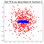
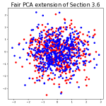
Figure 1: Fair PCA as described in Section 2 (left), which equalizes the group-conditional means, in comparison to the higher-order variant of Section 3.6 (right), which additionally aims to equalize the group-conditional covariance matrices. Only the higher-order variant completely obfuscates the demographic information (encoded by color: red vs. blue).

4 RELATED WORK

Fairness in machine learning (ML)

Most works study the problem of fair classification (e.g., Zafar et al., 2019), but fairness has also been studied for unsupervised learning tasks (e.g., Chierichetti et al., 2017). Two of the most prominent definitions of fairness in classification are demographic parity (Kamiran and Calders, 2011) and equal opportunity (Hardt et al., 2016) as introduced in Section 1. Methods for fair classification are commonly categorized into pre-processing, in-processing, and post-processing methods, depending on at which stage of the training pipeline they are applied (d’Alessandro et al., 2017). In the following we discuss the works most closely related to our paper, all of which can generally be considered as pre-processing methods.

Fair representation learning

Zemel et al. (2013) initiated the study of fair representation learning, where the goal is to learn an intermediate data representation that obfuscates demographic information while encoding other (non-demographic) information as well as possible. Once such a representation is found, any ML model trained on it should not be able to discriminate based on demographic information and hence be demographic parity fair. The approach of Zemel et al. learns prototypes and a probabilistic mapping of datapoints to these prototypes. Since then, numerous methods for fair representation learning have been proposed (e.g. Louizos et al., 2016; Moyer et al., 2018; Sarhan et al., 2020; Balunovic et al., 2022; Oh et al., 2022), many of them formulating the problem as an adversarial game (e.g. Edwards and Storkey, 2016; Beutel et al., 2017; Xie et al., 2017; Jia et al., 2018; Madras et al., 2018; Raff and Sylvester, 2018; Adel et al., 2019; Alvi et al., 2019; Feng et al., 2019; Song et al., 2019) and some of them adapting their approach to aim for downstream classifiers to be equal opportunity fair (e.g. Madras et al., 2018; Song et al., 2019). In contrast to our proposed approach, none of these techniques allows for an analytical solution and all of them require numerical optimization, which has often been found hard to perform, in particular for the adversarial approaches (cf. Feng et al., 2019, Sec. 5, or Oh et al., 2022, Sec. 2.2).

Fair PCA for fair representation learning and other methods for linear guarding

The methods discussed next are all methods for fair representation learning that bear some resemblance to our proposed approach. Most closely related to our work are the papers by Olfat and Aswani (2019), Lee et al. (2022), and Shao et al. (2022).

Olfat and Aswani (2019) introduced a notion of fair PCA with the same goal that we are aiming for in our formulation, that is finding a best-approximating projection such that no linear classifier can predict demographic information from the projected data. They use Pinsker’s inequality and an approximation of the group-conditional distributions by two Gaussians to obtain an upper bound on the best linear classifier’s accuracy. The upper bound is minimized when the projected data’s group-conditional means and covariance matrices coincide. Olfat and Aswani then formulate a semidefinite program (SDP) to minimize the projection’s reconstruction error while satisfying upper bounds on the differences in the projected data’s group-conditional means and covariance matrices. This SDP approach has been criticized by Lee et al. (2022, Section 5.1) for its high runtime and its relaxation of the rank constraint to a trace constraint, “yielding sub-optimal outputs in presence of (fairness) constraints, even to substantial order in some cases”. In Section 5 we rerun the experiments of Lee et al. and also observe that the running time of the method by Olfat and Aswani is prohibitively high. Furthermore, we consider our derivation of fair PCA to be more intuitive since we do not rely on upper bounds or a Gaussian approximation.

Arguing that matching only group-conditional means and covariance matrices of the projected data might be too weak of a constraint, Lee et al. (2022) define a version of fair PCA by requiring that the projected data’s group-conditional distributions coincide. They use the maximum mean discrepancy to measure the deviation of the group-conditional distributions and a penalty method for manifold optimization to solve the resulting optimization problem. While running much faster than the method by Olfat and Aswani (2019), we find the running time of the method by Lee et al. to be significantly higher than the running time of our proposed algorithms; still, in terms of the quality of the data representation our algorithms can compete. Lee et al. present their algorithm only for two demographic groups and it is unclear whether it can be extended to more than two groups.

Concurrently with the writing of our paper, Shao et al. (2022) proposed the spectral attribute removal (SAL) algorithm to remove demographic information via a data projection. Their algorithm is based on the observation that a singular value decomposition of the cross-covariance matrix between feature vector $\mathbf{x}$ and demographic attribute $z$ yields projections that maximize the covariance of $\mathbf{x}$ and $z$. Although derived differently, it turns out that the SAL algorithm and our fair PCA method are closely related: SAL projects the data onto the subspace spanned by the columns of the matrix $\mathbf{R}$ in our Algorithm 1. Hence, for $k=d-1$ the two algorithms project the data onto the same subspace. However, SAL does not allow to choose an embedding dimension smaller than $d-1$. While Shao et al. also provide a kernelized variant of their algorithm, they do not provide the interpretation of matching group-conditional means or any extension to also match group-conditional covariances.

There are also papers that propose methods for linear guarding, that is finding a data representation from which no linear classifier can predict demographic information, that are not related to PCA: Ravfogel et al. (2020) iteratively train a linear classifier to predict the demographic attribute and then project the data onto the classifier’s nullspace; Haghighatkhah et al. (2021) describe a procedure to find a projection such that the projected data is not linearly separable w.r.t. the demographic attribute anymore, but still linearly separable w.r.t. some other binary attributes; Ravfogel et al. (2022) formulate the problem of linear guarding as a linear minimax game, where a projection matrix competes against the parameter vector of a linear model. In case of linear regression this game can be solved analytically, while for logistic regression and other linear models a relaxation of the game is solved via alternate minimization and maximization.

Fair PCA for balancing reconstruction error

A very different notion of fair PCA was introduced by Samadi et al. (2018), which views PCA as a standalone problem and wants to balance the excess reconstruction error across different demographic groups. This line of work, which is incomparable to our notion of fair PCA and the notions discussed above, has been extended by Tantipongpipat et al. (2019), Pelegrina et al. (2021) and Kamani et al. (2022).

Information bottleneck method

As pointed out by one of the reviewers, there might be a closer relationship between our formulation of fair PCA and the information bottleneck method (Tishby et al., 1999), where the goal is to find a compression of a signal variable $X$ while preserving information about a relevance variable $Y$. In particular, when $X$ and $Y$ are jointly multivariate Gaussian variables, the optimal projection matrix is obtained by solving an eigenvalue problem involving the cross-covariance matrix $\mathbf{\Sigma}_{XY}=(\mathbb{E}[(X_{i}-\mathbb{E}[X_{i}])(Y_{j}-\mathbb{E}[Y_{j}])])_{ij}$ (Chechik et al., 2005).

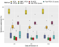
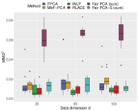
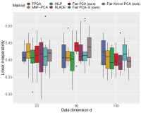
Figure 2: We compare our proposed algorithms to standard PCA and the methods by Olfat and Aswani (2019) (FPCA), Lee et al. (2022) (MbF-PCA), Ravfogel et al. (2020) (INLP), and Ravfogel et al. (2022) (RLACE), in the experimental setup of Lee et al.. Variance explained (left plot; higher is better) measures how well the representation approximates the data; MMD² (middle plot; lower is better) and linear inseparability (right plot; higher is better) measure the fairness of the representation—see the running text for details. The left and middle plots do not show results for fair kernel PCA since its projection space lies in a reproducing kernel Hilbert space (e.g., Schölkopf and Smola, 2002) and the two metrics are not comparable between fair kernel PCA and the other methods. The middle and right plots do not show results for standard PCA since its values are too high and low, respectively ($\text{MMD}^{2}>0.5$ and $\text{linear inseparability}<0.02$ for all data dimensions).

5 EXPERIMENTS

In this section, we present a number of experiments. We first rerun and extend the experiments performed by Lee et al. (2022) in order to compare our algorithms to the existing methods for fair PCA by Olfat and Aswani (2019) and Lee et al. (2022) and to the methods for linear guarding by Ravfogel et al. (2020) and Ravfogel et al. (2022). We also apply our version of fair PCA to the CelebA dataset of facial images to illustrate its applicability to large high-dimensional datasets. We then demonstrate the usefulness of our proposed algorithms as means of bias mitigation and compare their performance to the reductions approach of Agarwal et al. (2018), which is the state-of-the-art in-processing method implemented in Fairlearn (https://fairlearn.org/). Some implementation details and details about datasets are provided in Appendix C.1 and C.2.

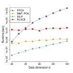
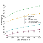
Figure 3: The running time of the various methods as a function of the data dimension $d$. The target dimension $k$ is 5 independent of $d$. Note the logarithmic y-axes and that the x-axes are different for the two plots.

Table 1: Comparison of our proposed algorithms with standard PCA and the fair methods FPCA, MbF-PCA, INLP, and RLACE on the Adult Income dataset in the setup of Lee et al. (2022). The top half shows the results for the target dimension $k=2$, the lower half for $k=10$. Within each block of methods (standard PCA / fair competitors / our fair methods) results with the best mean values are shown in bold. For fair kernel PCA, %Var and MMD² are not meaningful.

Adult Income [$\text{feature dim}=97$, $\operatorname{Pr}(Y=1)=0.2489$]
$k$	Algorithm	%Var($\uparrow$)	MMD2($\downarrow$)	%Acc($\uparrow$)	$\Delta_{DP}$($\downarrow$)	%Acc($\uparrow$)	$\Delta_{DP}$($\downarrow$)	%Acc($\uparrow$)	$\Delta_{DP}$($\downarrow$)
				Kernel SVM		Linear SVM		MLP
2	PCA	$\mathbf{7.78_{0.77}}$	$\mathbf{0.349_{0.026}}$	$\mathbf{82.03_{1.09}}$	$\mathbf{0.2_{0.05}}$	$\mathbf{79.87_{1.11}}$	$\mathbf{0.2_{0.04}}$	$\mathbf{81.21_{1.22}}$	$\mathbf{0.22_{0.03}}$
2-10	FPCA (0.1, 0.01)	$4.05_{0.93}$	$0.016_{0.011}$	$77.44_{2.81}$	$0.04_{0.03}$	$75.54_{1.98}$	$\mathbf{0.0_{0.0}}$	$76.19_{2.44}$	$0.02_{0.03}$
	FPCA (0, 0.01)	$3.65_{0.92}$	$0.005_{0.004}$	$77.05_{3.02}$	$\mathbf{0.01_{0.01}}$	$75.51_{1.93}$	$0.01_{0.02}$	$76.24_{2.81}$	$\mathbf{0.01_{0.01}}$
	MbF-PCA ($10^{-3}$)	$\mathbf{6.08_{0.59}}$	$0.005_{0.004}$	$\mathbf{79.46_{1.21}}$	$0.02_{0.01}$	$\mathbf{76.97_{1.71}}$	$0.02_{0.01}$	$\mathbf{78.6_{1.38}}$	$0.02_{0.02}$
	MbF-PCA ($10^{-6}$)	$5.83_{0.54}$	$0.005_{0.004}$	$79.12_{1.08}$	$\mathbf{0.01_{0.01}}$	$76.7_{1.86}$	$0.02_{0.02}$	$77.69_{1.46}$	$0.02_{0.01}$
	INLP	$2.09_{0.18}$	$\mathbf{0.003_{0.001}}$	$75.94_{1.4}$	$\mathbf{0.01_{0.01}}$	$75.11_{1.66}$	$\mathbf{0.0_{0.0}}$	$75.3_{1.68}$	$\mathbf{0.01_{0.01}}$
	RLACE	$1.98_{0.19}$	$0.007_{0.008}$	$76.24_{1.37}$	$0.02_{0.03}$	$75.11_{1.66}$	$\mathbf{0.0_{0.0}}$	$75.8_{1.31}$	$0.02_{0.02}$
2-10	Fair PCA	$\mathbf{6.37_{0.65}}$	$0.009_{0.003}$	$\mathbf{80.24_{1.57}}$	$0.06_{0.02}$	$\mathbf{77.26_{1.79}}$	$0.02_{0.02}$	$\mathbf{78.63_{1.36}}$	$0.04_{0.02}$
	Fair Kernel PCA	$n/a$	$n/a$	$75.11_{1.66}$	$\mathbf{0.0_{0.0}}$	$75.11_{1.66}$	$\mathbf{0.0_{0.0}}$	$77.08_{1.78}$	$0.03_{0.03}$
	Fair PCA-S (0.5)	$3.05_{0.3}$	$\mathbf{0.002_{0.002}}$	$75.85_{1.59}$	$0.01_{0.01}$	$75.11_{1.66}$	$\mathbf{0.0_{0.0}}$	$75.26_{1.63}$	$0.01_{0.01}$
	Fair PCA-S (0.85)	$4.27_{0.34}$	$0.003_{0.002}$	$76.07_{1.34}$	$0.01_{0.01}$	$75.11_{1.66}$	$\mathbf{0.0_{0.0}}$	$75.01_{1.76}$	$\mathbf{0.0_{0.01}}$
10	PCA	$\mathbf{21.77_{1.95}}$	$\mathbf{0.195_{0.006}}$	$\mathbf{93.64_{0.87}}$	$\mathbf{0.16_{0.01}}$	$\mathbf{82.68_{0.96}}$	$\mathbf{0.18_{0.02}}$	$\mathbf{89.06_{2.07}}$	$\mathbf{0.2_{0.03}}$
2-10	FPCA (0.1, 0.01)	$15.75_{1.14}$	$0.006_{0.003}$	$91.94_{0.84}$	$0.13_{0.02}$	$78.1_{2.15}$	$0.03_{0.02}$	$\mathbf{87.17_{1.1}}$	$0.11_{0.04}$
	FPCA (0, 0.01)	$15.52_{1.12}$	$0.004_{0.002}$	$91.66_{0.92}$	$0.13_{0.02}$	$77.72_{2.06}$	$0.03_{0.02}$	$85.38_{2.08}$	$0.09_{0.03}$
	MbF-PCA ($10^{-3}$)	$\mathbf{18.86_{1.46}}$	$0.005_{0.002}$	$\mathbf{93.06_{0.85}}$	$0.15_{0.01}$	$\mathbf{80.53_{1.31}}$	$0.03_{0.02}$	$86.83_{2.05}$	$0.08_{0.03}$
	MbF-PCA ($10^{-6}$)	$12.36_{4.15}$	$\mathbf{0.002_{0.001}}$	$83.58_{3.58}$	$\mathbf{0.05_{0.02}}$	$75.11_{1.66}$	$\mathbf{0.0_{0.0}}$	$80.27_{3.55}$	$\mathbf{0.04_{0.04}}$
	INLP	$10.79_{0.84}$	$0.004_{0.001}$	$89.01_{1.19}$	$0.1_{0.03}$	$75.11_{1.66}$	$\mathbf{0.0_{0.0}}$	$85.24_{1.2}$	$0.11_{0.03}$
	RLACE	$10.3_{0.49}$	$0.007_{0.005}$	$90.96_{1.04}$	$0.12_{0.04}$	$75.11_{1.66}$	$\mathbf{0.0_{0.0}}$	$86.61_{1.69}$	$0.11_{0.05}$
2-10	Fair PCA	$\mathbf{19.62_{1.73}}$	$0.014_{0.003}$	$\mathbf{93.42_{0.8}}$	$0.16_{0.01}$	$\mathbf{81.31_{1.23}}$	$0.04_{0.02}$	$\mathbf{88.16_{1.45}}$	$0.16_{0.03}$
	Fair Kernel PCA	$n/a$	$n/a$	$79.9_{1.54}$	$\mathbf{0.04_{0.03}}$	$78.34_{1.21}$	$0.02_{0.02}$	$80.52_{2.05}$	$\mathbf{0.06_{0.03}}$
	Fair PCA-S (0.5)	$12.75_{1.31}$	$\mathbf{0.004_{0.001}}$	$86.85_{1.79}$	$0.09_{0.02}$	$75.11_{1.66}$	$\mathbf{0.0_{0.0}}$	$82.89_{2.01}$	$0.07_{0.04}$
	Fair PCA-S (0.85)	$15.79_{1.05}$	$0.005_{0.001}$	$91.81_{1.05}$	$0.15_{0.02}$	$75.11_{1.66}$	$\mathbf{0.0_{0.0}}$	$87.07_{1.4}$	$0.15_{0.02}$

5.1 Comparison with Existing Methods for Fair PCA

Experiments as in Lee et al. (2022)

We used the code provided by Lee et al. (2022) to rerun their experiments and perform a comparison with our proposed algorithms. We additionally compared to the methods by Ravfogel et al. (2020) and Ravfogel et al. (2022) using the code provided by those authors, where we set all parameters to their default values except for the maximum number of outer iterations for the second method, which we decreased from 75000 to 10000 to get a somewhat acceptable running time. We extended the experimental evaluation of Lee et al. by reporting additional metrics, but other than that did not modify their code or experimental setting in any way.

In their first experiment (Section 8.2 in their paper), Lee et al. (2022) applied standard PCA, their method (referred to as MbF-PCA) and the method by Olfat and Aswani (2019) (FPCA) to synthetic data sampled from a mixture of two Gaussians of varying dimension $d$. The two Gaussians correspond to two demographic groups. The target dimension $k$ is held constant at $5$. We reran the code of Lee et al. and additionally applied the methods of Ravfogel et al. (2020) (INLP) and Ravfogel et al. (2022) (RLACE) and our algorithms for fair PCA, fair kernel PCA with a Gaussian kernel, and the variant of fair PCA that additionally aims to equalize group-conditional covariance matrices (referred to as Fair PCA-S; we set $l=\lfloor 0.85d\rfloor$—cf. Section 3.6). Lee et al. reported the fraction of explained variance of the projected data (i.e., $\operatorname{trace}(\mathbf{U}^{\mathchoice{\raisebox{0.0pt}{$\displaystyle\intercal$}}{\raisebox{0.0pt}{$\textstyle\intercal$}}{\raisebox{0.0pt}{$\scriptstyle\intercal$}}{\raisebox{0.0pt}{$\scriptscriptstyle\intercal$}}}\mathbf{X}\mathbf{X}^{\mathchoice{\raisebox{0.0pt}{$\displaystyle\intercal$}}{\raisebox{0.0pt}{$\textstyle\intercal$}}{\raisebox{0.0pt}{$\scriptstyle\intercal$}}{\raisebox{0.0pt}{$\scriptscriptstyle\intercal$}}}\mathbf{U})/\operatorname{trace}(\mathbf{X}\mathbf{X}^{\mathchoice{\raisebox{0.0pt}{$\displaystyle\intercal$}}{\raisebox{0.0pt}{$\textstyle\intercal$}}{\raisebox{0.0pt}{$\scriptstyle\intercal$}}{\raisebox{0.0pt}{$\scriptscriptstyle\intercal$}}})$ for the projection defined by $\mathbf{U}$—higher means better approximation of the original data), the squared maximum mean discrepancy (MMD²) based on a Gaussian kernel between the two groups after the projection (lower means the representation is more fair) and the running time of the methods. We additionally report the error of a linear classifier trained to predict the demographic information from the projected data (higher means the representation is more fair; we refer to this metric as linear inseparability). Figure 2 and Figure 4 show the results, where the boxplots are obtained from considering ten random splits into training and test data and the runtime curves show an average over the ten splits. While standard PCA does best in approximating the original data (variance about 50%), it does not yield a fair representation with high values for MMD² (more than 0.5) and low values for linear inseparability ($\approx 0$). Our algorithm for fair PCA does worse in approximating the data (variance above 30%), but drastically reduces the unfairness of standard PCA (MMD² smaller than 0.07). The other methods yield even lower values for MMD², but this comes at the cost of a worse approximation of the data. Our variant Fair PCA-S performs similarly to FPCA by Olfat and Aswani (2019). All methods except standard PCA perform similarly in terms of linear inseparability. The biggest difference is in the methods’ running times: while FPCA runs for more than 2000 seconds, RLACE for about 20 seconds, MbF-PCA for about 1.3 seconds, and INLP for about 0.8 seconds when the data dimension $d$ is as small as 100, none of our algorithms runs for more than 0.5 seconds even when $d=800$. In the latter case, RLACE runs for about 260 seconds, MbF-PCA for about 43 seconds, and INLP for about 1270 seconds. In Appendix C.3, we study the running time of the methods as a function of the target dimension $k$ and observe that the running time of MbF-PCA drastically increases with $k$ (about 290 seconds when $d=100$ and $k=50$). This shows that none of the existing methods can be applied when both $d$ and $k$ are large (such as in the experiment on the CelebA dataset below) and provides strong evidence for the benefit of our proposed methods.

In their second experiment (Section 8.3 in their paper), Lee et al. (2022) applied standard PCA, MbF-PCA and FPCA to three real-world datasets: Adult Income and German Credit from the UCI repository (Dua and Graff, 2017), and COMPAS (Angwin et al., 2016). Lee et al. ran MbF-PCA and FPCA for two different parameter configurations, indicated by the numbers in parentheses after a method’s name in the tables below. Similarly, we ran our proposed method Fair PCA-S from Section 3.6 for $l=\max\{k,\lfloor 0.5d\rfloor\}$ as well as $l=\max\{k,\lfloor 0.85d\rfloor\}$. Lee et al. reported the explained variance and MMD² as above. Furthermore, they reported the accuracy and the DP violation $\Delta_{DP}:=|\operatorname{Pr}(\hat{Y}=1|Z=0)-\operatorname{Pr}(\hat{Y}=1|Z=1)|$ of a Gaussian kernel support vector machine (SVM) trained to solve a downstream task on the projected data (e.g., for the Adult Income dataset the downstream task is to predict whether a person’s income exceeds $50k or not). We additionally report the accuracy and $\Delta_{DP}$ of a linear SVM and a multilayer perceptron (MLP) with two hidden layers of size 10 and 5, respectively. Table 1 provides the results for Adult Income; the tables for German Credit and COMPAS can be found in Appendix C.4. The reported results are average results (together with standard deviations in subscript) over ten random splits into training and test data. We see that there is no single best method. Methods that allow for a high downstream accuracy tend to suffer from higher DP violation and the other way around. The parameters of FPCA and MbF-PCA allow to trade-off accuracy vs. fairness and so does the parameter $l$ in Fair PCA-S (note that Fair PCA is equivalent to Fair PCA-S(1.0)). Except on COMPAS, whose data dimension is very small, Fair PCA-S always achieves smaller DP violation than fair PCA for the non-linear classifiers and fair kernel PCA achieves the smallest DP violation, among all methods, for the kernel SVM. Overall, we consider the results for our proposed methods to be similar as for the existing methods.

One of the reviewers asked for a comparison with the method of Samadi et al. (2018), which aims to balance the excess reconstruction error of PCA across different demographic groups (cf. Section 4). We emphasize once more that this fairness notion is incomparable to ours (also see the discussion in Appendix A of Lee et al., 2022). Still, we provide the results for the method of Samadi et al. (2018) on the three real-world datasets in Appendix C.5. As expected, their method yields much higher DP violations than our methods or the other competitors.

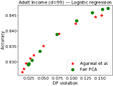
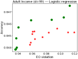
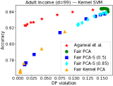
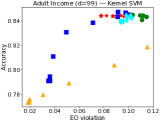
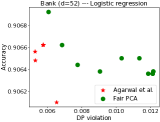
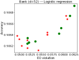
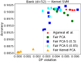
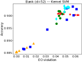
Figure 4: We compare our proposed algorithms, used as pre-processing methods for bias mitigation, to the state-of-the-art in-processing method of Agarwal et al. (2018). The first row shows results for the Adult Income dataset, the second row for the Bank Marketing dataset. Our algorithms generate comparable trade-off curves, but run much faster (cf. Appendix C.7).

Original

dim$=$6400

 

Fair PCA

$k=6399$

Fair PCA

$k=400$

Figure 5: Fair PCA applied to the CelebA dataset to erase the concept of “glasses”. See App. C.6 for more examples.

Applying fair PCA to CelebA similarly to Ravfogel et al. (2022)

Similarly to Ravfogel et al. (2022), we applied our fair PCA method to the CelebA dataset (Liu et al., 2015) to erase concepts such as “glasses” or “mustache” from facial images. The CelebA dataset comprises 202599 pictures of faces of celebrities. We rescaled all images to $80\times 80$ grey-scale images and applied our Algorithm 1 to the flattened raw-pixel vectors, using one of the bald, beard, eyeglasses, hat, mustache, or smiling annotations as demographic attributes. Figure 5 shows some results for eyeglasses; we provide more results, also for the other attributes, and a discussion in Appendix C.6. Due to their high running time, we were not able to apply the methods by Olfat and Aswani (2019), Lee et al. (2022), Ravfogel et al. (2020), or Ravfogel et al. (2022) to this large and high-dimensional dataset. However, results for the method of Ravfogel et al. (2022) for a smaller resolution can be found in their paper.

5.2 Comparison with Agarwal et al. (2018)

We compare our proposed algorithms as means of bias mitigation to the state-of-the-art in-processing method of Agarwal et al. (2018). While our algorithms learn a fair representation and perform standard training (without fairness considerations) on top of that representation to learn a fair classifier, the approach of Agarwal et al. modifies the training procedure. Concretely, their approach solves a sequence of cost-sensitive classification problems. We apply the various methods to the Adult Income and the Bank Marketing dataset (Moro et al., 2014), which are both available on the UCI repository (Dua and Graff, 2017). The goal for each method is to produce good accuracy vs. fairness trade-off curves—every point on a trade-off curve corresponds to a specific classifier. Note that the approach of Agarwal et al. yields randomized classifiers, which is problematic if a classifier strongly affects humans’ lives (Cotter et al., 2019). For our algorithms we deploy the strategy of Section 3.1 to produce the trade-off curves. Figure 4 shows the results. All results are average results obtained from considering ten random draws of train and test data (see Appendix C.2 for details). The plots show on the y-axis the accuracy of a classifier and on the x-axis its fairness violation, which is $\Delta_{DP}=|\operatorname{Pr}(\hat{Y}=1|Z=0)-\operatorname{Pr}(\hat{Y}=1|Z=1)|$ as in Section 5.1 when aiming for DP and $\Delta_{EO}:=|\operatorname{Pr}(\hat{Y}=1|Z=0,Y=1)-\operatorname{Pr}(\hat{Y}=1|Z=1,Y=1)|$ when aiming for EO. In the first and the second plot of each row we learn a logistic regression classifier, aiming to satisfy DP or EO. We see that fair PCA produces similar curves as the method by Agarwal et al. (note that in the bottom left plot $\Delta_{DP}$ is very small for all classifiers). However, fair PCA runs much faster: including the classifier training, fair PCA runs for 0.04 seconds on average while the method by Agarwal et al. runs for 4.6 seconds (see Appendix C.7 for details). These plots do not show results for Fair PCA-S and fair kernel PCA since they cannot compete (we provide those results in Appendix C.7). Fair PCA-S and fair kernel PCA can compete when training a kernel SVM classifier though (third and fourth plot of each row).

6 DISCUSSION

We provided a new derivation of fair PCA, aiming for a fair representation that does not contain demographic information. Our derivation is simple and allows for efficient algorithms based on eigenvector computations similar to standard PCA. Compared to existing methods for fair PCA, our proposed algorithms run much faster while achieving similar results. In a comparison with a state-of-the-art in-processing bias mitigation method we saw that our algorithms provide a significantly faster alternative to train fair classifiers.

APPENDIX

Appendix A ADDENDUM TO SECTION 2

A.1 Problem (3) May Not Be Well Defined

Let $n=2n^{\prime}$, $\mathbf{x}_{1}=\mathbf{x}_{2}=\ldots=\mathbf{x}_{n^{\prime}}=\mathbf{0}\in\mathbb{R}^{2}$, and $\mathbf{x}_{n^{\prime}+1},\ldots\mathbf{x}_{2n^{\prime}}\in\mathbb{R}^{2}$ be equidistantly spread on a circle with center $\mathbf{0}$. Let $z_{1}=\ldots=z_{n^{\prime}}=0$, $z_{n^{\prime}+1}=\ldots=z_{2n^{\prime}}=1$, and $k=1$. Any projection onto a 1-dimensional linear subspace maps $\mathbf{x}_{1},\ldots,\mathbf{x}_{n^{\prime}}$ to $\mathbf{0}$ and $\mathbf{x}_{n^{\prime}+1},\ldots,\mathbf{x}_{2n^{\prime}}$ onto a line through $\mathbf{0}$ such that half the points of $\mathbf{x}_{n^{\prime}+1},\ldots,\mathbf{x}_{2n^{\prime}}$ lie on one side of $\mathbf{0}$ and the other half lies on the other side of $\mathbf{0}$ (at most two of $\mathbf{x}_{n^{\prime}+1},\ldots,\mathbf{x}_{2n^{\prime}}$ might map to $\mathbf{0}$). The function $h:\mathbb{R}\rightarrow\mathbb{R}$ with $h(x)=\mathds{1}[x\neq 0]$ (almost) perfectly predicts $z_{i}$ from the projected points, showing that the set $\mathcal{U}$ defined in (3) can be empty if we require $h(\mathbf{U}^{\mathchoice{\raisebox{0.0pt}{$\displaystyle\intercal$}}{\raisebox{0.0pt}{$\textstyle\intercal$}}{\raisebox{0.0pt}{$\scriptstyle\intercal$}}{\raisebox{0.0pt}{$\scriptscriptstyle\intercal$}}}\mathbf{x}_{i})$ and $z_{i}$ to be independent for all functions $h$.

The same example shows that $\mathcal{U}$ can be empty if we require $h(\mathbf{U}^{\mathchoice{\raisebox{0.0pt}{$\displaystyle\intercal$}}{\raisebox{0.0pt}{$\textstyle\intercal$}}{\raisebox{0.0pt}{$\scriptstyle\intercal$}}{\raisebox{0.0pt}{$\scriptscriptstyle\intercal$}}}\mathbf{x}_{i})$ and $z_{i}$ to be uncorrelated (rather than independent) for all functions $h$.

It also shows that $\mathcal{U}$ can be empty if we require $h(\mathbf{U}^{\mathchoice{\raisebox{0.0pt}{$\displaystyle\intercal$}}{\raisebox{0.0pt}{$\textstyle\intercal$}}{\raisebox{0.0pt}{$\scriptstyle\intercal$}}{\raisebox{0.0pt}{$\scriptscriptstyle\intercal$}}}\mathbf{x}_{i})$ and $z_{i}$ to be independent for all linear functions $h$ (rather than all functions $h$): for $h:\mathbb{R}\rightarrow\mathbb{R}$ with $h(x)=x$, $h(\mathbf{U}^{\mathchoice{\raisebox{0.0pt}{$\displaystyle\intercal$}}{\raisebox{0.0pt}{$\textstyle\intercal$}}{\raisebox{0.0pt}{$\scriptstyle\intercal$}}{\raisebox{0.0pt}{$\scriptscriptstyle\intercal$}}}\mathbf{x}_{i})$ and $z_{i}$ are clearly dependent.

This shows that we have to relax Problem (3) in two ways in order to arrive at a well defined problem.

Algorithm 2 Fair PCA (for multiple demographic groups)

  Input: data matrix $\mathbf{X}\in\mathbb{R}^{d\times n}$; demographic attributes $z_{i}^{(1)},\ldots,z_{i}^{(m)}\in\{0,1\}$, $i\in[n]$, where $z_{i}^{(l)}$ encodes membership of the $i$-th datapoint in the $l$-th group; target dimension $k\in[d-m+1]$

  Output: a solution $\mathbf{U}$ to the multi-group version of Problem (4)

• set $\mathbf{Z}\in\mathbb{R}^{n\times m}$ with the $l$-th column of $\mathbf{Z}$ equaling $(z_{1}^{(l)}-\bar{z}^{(l)},\ldots,z_{n}^{(l)}-\bar{z}^{(l)})^{\mathchoice{\raisebox{0.0pt}{$\displaystyle\intercal$}}{\raisebox{0.0pt}{$\textstyle\intercal$}}{\raisebox{0.0pt}{$\scriptstyle\intercal$}}{\raisebox{0.0pt}{$\scriptscriptstyle\intercal$}}}$ with $\bar{z}^{(l)}=\frac{1}{n}\sum_{i=1}^{n}z_{i}^{(l)}$

• compute an orthonormal basis of the nullspace of $\mathbf{Z}^{\mathchoice{\raisebox{0.0pt}{$\displaystyle\intercal$}}{\raisebox{0.0pt}{$\textstyle\intercal$}}{\raisebox{0.0pt}{$\scriptstyle\intercal$}}{\raisebox{0.0pt}{$\scriptscriptstyle\intercal$}}}\mathbf{X}^{\mathchoice{\raisebox{0.0pt}{$\displaystyle\intercal$}}{\raisebox{0.0pt}{$\textstyle\intercal$}}{\raisebox{0.0pt}{$\scriptstyle\intercal$}}{\raisebox{0.0pt}{$\scriptscriptstyle\intercal$}}}$ and build matrix $\mathbf{R}$ comprising the basis vectors as columns

• compute orthonormal eigenvectors, corresponding to the largest $k$ eigenvalues, of $\mathbf{R}^{\mathchoice{\raisebox{0.0pt}{$\displaystyle\intercal$}}{\raisebox{0.0pt}{$\textstyle\intercal$}}{\raisebox{0.0pt}{$\scriptstyle\intercal$}}{\raisebox{0.0pt}{$\scriptscriptstyle\intercal$}}}\mathbf{X}\mathbf{X}^{\mathchoice{\raisebox{0.0pt}{$\displaystyle\intercal$}}{\raisebox{0.0pt}{$\textstyle\intercal$}}{\raisebox{0.0pt}{$\scriptstyle\intercal$}}{\raisebox{0.0pt}{$\scriptscriptstyle\intercal$}}}\mathbf{R}$ and build matrix $\mathbf{\Lambda}$ comprising the eigenvectors as columns

• return $\mathbf{U}=\mathbf{R}\mathbf{\Lambda}$

Appendix B ADDENDUM TO SECTION 3

B.1 Fair PCA for Multiple Demographic Groups

In fair PCA for multiple groups we want to solve

$$\operatorname{argmax}_{\mathbf{U}\in\mathbb{R}^{d\times k}:\,\mathbf{U}^{\mathchoice{\raisebox{0.0pt}{$\displaystyle\intercal$}}{\raisebox{0.0pt}{$\textstyle\intercal$}}{\raisebox{0.0pt}{$\scriptstyle\intercal$}}{\raisebox{0.0pt}{$\scriptscriptstyle\intercal$}}}\mathbf{U}=\mathbf{I}_{k\times k}}\operatorname{trace}(\mathbf{U}^{\mathchoice{\raisebox{0.0pt}{$\displaystyle\intercal$}}{\raisebox{0.0pt}{$\textstyle\intercal$}}{\raisebox{0.0pt}{$\scriptstyle\intercal$}}{\raisebox{0.0pt}{$\scriptscriptstyle\intercal$}}}\mathbf{X}\mathbf{X}^{\mathchoice{\raisebox{0.0pt}{$\displaystyle\intercal$}}{\raisebox{0.0pt}{$\textstyle\intercal$}}{\raisebox{0.0pt}{$\scriptstyle\intercal$}}{\raisebox{0.0pt}{$\scriptscriptstyle\intercal$}}}\mathbf{U})\quad\text{subject to}\quad\mathbf{Z}^{\mathchoice{\raisebox{0.0pt}{$\displaystyle\intercal$}}{\raisebox{0.0pt}{$\textstyle\intercal$}}{\raisebox{0.0pt}{$\scriptstyle\intercal$}}{\raisebox{0.0pt}{$\scriptscriptstyle\intercal$}}}\mathbf{X}^{\mathchoice{\raisebox{0.0pt}{$\displaystyle\intercal$}}{\raisebox{0.0pt}{$\textstyle\intercal$}}{\raisebox{0.0pt}{$\scriptstyle\intercal$}}{\raisebox{0.0pt}{$\scriptscriptstyle\intercal$}}}\mathbf{U}=\mathbf{0},$$ (10)

where $\mathbf{Z}\in\mathbb{R}^{n\times m}$ and the $l$-th column of $\mathbf{Z}$ equals $(z_{1}^{(l)}-\bar{z}^{(l)},\ldots,z_{n}^{(l)}-\bar{z}^{(l)})^{\mathchoice{\raisebox{0.0pt}{$\displaystyle\intercal$}}{\raisebox{0.0pt}{$\textstyle\intercal$}}{\raisebox{0.0pt}{$\scriptstyle\intercal$}}{\raisebox{0.0pt}{$\scriptscriptstyle\intercal$}}}$ with $\bar{z}^{(l)}=\frac{1}{n}\sum_{i=1}^{n}z_{i}^{(l)}$ and $z_{i}^{(l)}=1$ if $\mathbf{x}_{i}$ belongs to group $l$ and $z_{i}^{(l)}=0$ otherwise. Assuming that no group is empty, the rank of $\mathbf{Z}$ is $m-1$ as $\sum_{l=1}^{m}\mathbf{Z}^{(l)}_{i}=0$, $i\in[n]$, and in any linear combination of $(m-1)$ many columns of $\mathbf{Z}$ equaling zero all coefficients must be zero. Hence, $\operatorname{rank}(\mathbf{Z}^{\mathchoice{\raisebox{0.0pt}{$\displaystyle\intercal$}}{\raisebox{0.0pt}{$\textstyle\intercal$}}{\raisebox{0.0pt}{$\scriptstyle\intercal$}}{\raisebox{0.0pt}{$\scriptscriptstyle\intercal$}}}\mathbf{X}^{\mathchoice{\raisebox{0.0pt}{$\displaystyle\intercal$}}{\raisebox{0.0pt}{$\textstyle\intercal$}}{\raisebox{0.0pt}{$\scriptstyle\intercal$}}{\raisebox{0.0pt}{$\scriptscriptstyle\intercal$}}})\leq\operatorname{rank}(\mathbf{Z}^{\mathchoice{\raisebox{0.0pt}{$\displaystyle\intercal$}}{\raisebox{0.0pt}{$\textstyle\intercal$}}{\raisebox{0.0pt}{$\scriptstyle\intercal$}}{\raisebox{0.0pt}{$\scriptscriptstyle\intercal$}}})=\operatorname{rank}(\mathbf{Z})=m-1$ and the nullspace of $\mathbf{Z}^{\mathchoice{\raisebox{0.0pt}{$\displaystyle\intercal$}}{\raisebox{0.0pt}{$\textstyle\intercal$}}{\raisebox{0.0pt}{$\scriptstyle\intercal$}}{\raisebox{0.0pt}{$\scriptscriptstyle\intercal$}}}\mathbf{X}^{\mathchoice{\raisebox{0.0pt}{$\displaystyle\intercal$}}{\raisebox{0.0pt}{$\textstyle\intercal$}}{\raisebox{0.0pt}{$\scriptstyle\intercal$}}{\raisebox{0.0pt}{$\scriptscriptstyle\intercal$}}}$ has dimension at least $d-m+1$. Let $\mathbf{R}\in\mathbb{R}^{d\times s}$ with $s\geq d-m+1$ comprise as columns an orthonormal basis of the nullspace of $\mathbf{Z}^{\mathchoice{\raisebox{0.0pt}{$\displaystyle\intercal$}}{\raisebox{0.0pt}{$\textstyle\intercal$}}{\raisebox{0.0pt}{$\scriptstyle\intercal$}}{\raisebox{0.0pt}{$\scriptscriptstyle\intercal$}}}\mathbf{X}^{\mathchoice{\raisebox{0.0pt}{$\displaystyle\intercal$}}{\raisebox{0.0pt}{$\textstyle\intercal$}}{\raisebox{0.0pt}{$\scriptstyle\intercal$}}{\raisebox{0.0pt}{$\scriptscriptstyle\intercal$}}}$. We can then substitute $\mathbf{U}=\mathbf{R}\mathbf{\Lambda}$ for $\mathbf{\Lambda}\in\mathbb{R}^{s\times k}$. The constraint $\mathbf{U}^{\mathchoice{\raisebox{0.0pt}{$\displaystyle\intercal$}}{\raisebox{0.0pt}{$\textstyle\intercal$}}{\raisebox{0.0pt}{$\scriptstyle\intercal$}}{\raisebox{0.0pt}{$\scriptscriptstyle\intercal$}}}\mathbf{U}=\mathbf{I}_{k\times k}$ becomes $\mathbf{\Lambda}^{\mathchoice{\raisebox{0.0pt}{$\displaystyle\intercal$}}{\raisebox{0.0pt}{$\textstyle\intercal$}}{\raisebox{0.0pt}{$\scriptstyle\intercal$}}{\raisebox{0.0pt}{$\scriptscriptstyle\intercal$}}}\mathbf{\Lambda}=\mathbf{I}_{k\times k}$, and the objective $\operatorname{trace}(\mathbf{U}^{\mathchoice{\raisebox{0.0pt}{$\displaystyle\intercal$}}{\raisebox{0.0pt}{$\textstyle\intercal$}}{\raisebox{0.0pt}{$\scriptstyle\intercal$}}{\raisebox{0.0pt}{$\scriptscriptstyle\intercal$}}}\mathbf{X}\mathbf{X}^{\mathchoice{\raisebox{0.0pt}{$\displaystyle\intercal$}}{\raisebox{0.0pt}{$\textstyle\intercal$}}{\raisebox{0.0pt}{$\scriptstyle\intercal$}}{\raisebox{0.0pt}{$\scriptscriptstyle\intercal$}}}\mathbf{U})$ becomes $\operatorname{trace}(\mathbf{\Lambda}^{\mathchoice{\raisebox{0.0pt}{$\displaystyle\intercal$}}{\raisebox{0.0pt}{$\textstyle\intercal$}}{\raisebox{0.0pt}{$\scriptstyle\intercal$}}{\raisebox{0.0pt}{$\scriptscriptstyle\intercal$}}}\mathbf{R}^{\mathchoice{\raisebox{0.0pt}{$\displaystyle\intercal$}}{\raisebox{0.0pt}{$\textstyle\intercal$}}{\raisebox{0.0pt}{$\scriptstyle\intercal$}}{\raisebox{0.0pt}{$\scriptscriptstyle\intercal$}}}\mathbf{X}\mathbf{X}^{\mathchoice{\raisebox{0.0pt}{$\displaystyle\intercal$}}{\raisebox{0.0pt}{$\textstyle\intercal$}}{\raisebox{0.0pt}{$\scriptstyle\intercal$}}{\raisebox{0.0pt}{$\scriptscriptstyle\intercal$}}}\mathbf{R}\mathbf{\Lambda})$. Hence, we can compute $\mathbf{\Lambda}$ by computing eigenvectors, corresponding to the largest $k$ eigenvalues, of $\mathbf{R}^{\mathchoice{\raisebox{0.0pt}{$\displaystyle\intercal$}}{\raisebox{0.0pt}{$\textstyle\intercal$}}{\raisebox{0.0pt}{$\scriptstyle\intercal$}}{\raisebox{0.0pt}{$\scriptscriptstyle\intercal$}}}\mathbf{X}\mathbf{X}^{\mathchoice{\raisebox{0.0pt}{$\displaystyle\intercal$}}{\raisebox{0.0pt}{$\textstyle\intercal$}}{\raisebox{0.0pt}{$\scriptstyle\intercal$}}{\raisebox{0.0pt}{$\scriptscriptstyle\intercal$}}}\mathbf{R}$. This requires $k\leq s$, which is guaranteed to hold for $k\leq d-m+1$.

If $m=2$, then the first and the second column of $\mathbf{Z}$ coincide up to multiplication by $-1$ and the nullspace of $\mathbf{Z}^{\mathchoice{\raisebox{0.0pt}{$\displaystyle\intercal$}}{\raisebox{0.0pt}{$\textstyle\intercal$}}{\raisebox{0.0pt}{$\scriptstyle\intercal$}}{\raisebox{0.0pt}{$\scriptscriptstyle\intercal$}}}\mathbf{X}^{\mathchoice{\raisebox{0.0pt}{$\displaystyle\intercal$}}{\raisebox{0.0pt}{$\textstyle\intercal$}}{\raisebox{0.0pt}{$\scriptstyle\intercal$}}{\raisebox{0.0pt}{$\scriptscriptstyle\intercal$}}}$ is the same as if we removed one of the two columns from $\mathbf{Z}$. This shows that for two groups, fair PCA as presented here is equivalent to fair PCA as presented in Section 2.

Finally, the interpretation of fair PCA provided in Section 2 also applies to the case of multiple groups: $\mathbf{Z}^{\mathchoice{\raisebox{0.0pt}{$\displaystyle\intercal$}}{\raisebox{0.0pt}{$\textstyle\intercal$}}{\raisebox{0.0pt}{$\scriptstyle\intercal$}}{\raisebox{0.0pt}{$\scriptscriptstyle\intercal$}}}\mathbf{X}^{\mathchoice{\raisebox{0.0pt}{$\displaystyle\intercal$}}{\raisebox{0.0pt}{$\textstyle\intercal$}}{\raisebox{0.0pt}{$\scriptstyle\intercal$}}{\raisebox{0.0pt}{$\scriptscriptstyle\intercal$}}}\mathbf{U}=\mathbf{0}$ is equivalent to

$$\frac{1}{|\{i:\mathbf{x}_{i}\in\text{group $l$}\}|}\sum_{i:\,\mathbf{x}_{i}\,\in\,\text{group $l$}}\mathbf{U}^{\mathchoice{\raisebox{0.0pt}{$\displaystyle\intercal$}}{\raisebox{0.0pt}{$\textstyle\intercal$}}{\raisebox{0.0pt}{$\scriptstyle\intercal$}}{\raisebox{0.0pt}{$\scriptscriptstyle\intercal$}}}\mathbf{x}_{i}=\frac{1}{|\{i:\mathbf{x}_{i}\notin\text{group $l$}\}|}\sum_{i:\,\mathbf{x}_{i}\,\notin\,\text{group $l$}}\mathbf{U}^{\mathchoice{\raisebox{0.0pt}{$\displaystyle\intercal$}}{\raisebox{0.0pt}{$\textstyle\intercal$}}{\raisebox{0.0pt}{$\scriptstyle\intercal$}}{\raisebox{0.0pt}{$\scriptscriptstyle\intercal$}}}\mathbf{x}_{i},\quad l=1,\ldots,m,$$

which in turn is equivalent to the projected data’s group-conditional means to coincide for all groups. Hence, an analogous version of Proposition 1 holds true for multiple groups.

The pseudo code of fair PCA for multiple demographic groups is provided in Algorithm 2. The pseudo code of fair kernel PCA for multiple demographic groups is provided in Algorithm 3.

Algorithm 3 Fair Kernel PCA (for multiple demographic groups)

  Input: kernel matrix $\mathbf{K}\in\mathbb{R}^{n\times n}$ with $\mathbf{K}_{ij}=k(\mathbf{x}_{i},\mathbf{x}_{j})$ for some kernel function $k$; demographic attributes $z_{i}^{(1)},\ldots,z_{i}^{(m)}\in\{0,1\}$, $i\in[n]$, where $z_{i}^{(l)}$ encodes membership of $\mathbf{x}_{i}$ in the $l$-th group; target dimension $k\in[n-m+1]$; optional: kernel matrix $\mathbf{\hat{K}}\in\mathbb{R}^{n\times n^{\prime}}$ with $\mathbf{\hat{K}}_{ij}=k(\mathbf{x}_{i},\mathbf{x}^{\prime}_{j})$, $i\in[n],j\in[n^{\prime}]$, for test data $\mathbf{x}^{\prime}_{1},\ldots,\mathbf{x}^{\prime}_{n^{\prime}}$

  Output: $k$-dimensional representation of the training data $\mathbf{x}_{1},\ldots,\mathbf{x}_{n}$; optional: $k$-dimensional representation of the test data $\mathbf{x}^{\prime}_{1},\ldots,\mathbf{x}^{\prime}_{n^{\prime}}$

• set $\mathbf{Z}\in\mathbb{R}^{n\times m}$ with the $l$-th column of $\mathbf{Z}$ equaling $(z_{1}^{(l)}-\bar{z}^{(l)},\ldots,z_{n}^{(l)}-\bar{z}^{(l)})^{\mathchoice{\raisebox{0.0pt}{$\displaystyle\intercal$}}{\raisebox{0.0pt}{$\textstyle\intercal$}}{\raisebox{0.0pt}{$\scriptstyle\intercal$}}{\raisebox{0.0pt}{$\scriptscriptstyle\intercal$}}}$ with $\bar{z}^{(l)}=\frac{1}{n}\sum_{i=1}^{n}z_{i}^{(l)}$

• compute an orthonormal basis of the nullspace of $\mathbf{Z}^{\mathchoice{\raisebox{0.0pt}{$\displaystyle\intercal$}}{\raisebox{0.0pt}{$\textstyle\intercal$}}{\raisebox{0.0pt}{$\scriptstyle\intercal$}}{\raisebox{0.0pt}{$\scriptscriptstyle\intercal$}}}\mathbf{K}$ and build matrix $\mathbf{R}$ comprising the basis vectors as columns

• compute orthonormal eigenvectors, corresponding to the largest $k$ eigenvalues, of the generalized eigenvalue problem $\mathbf{R}^{\mathchoice{\raisebox{0.0pt}{$\displaystyle\intercal$}}{\raisebox{0.0pt}{$\textstyle\intercal$}}{\raisebox{0.0pt}{$\scriptstyle\intercal$}}{\raisebox{0.0pt}{$\scriptscriptstyle\intercal$}}}\mathbf{K}\mathbf{K}\mathbf{R}\mathbf{\Lambda}=\mathbf{R}^{\mathchoice{\raisebox{0.0pt}{$\displaystyle\intercal$}}{\raisebox{0.0pt}{$\textstyle\intercal$}}{\raisebox{0.0pt}{$\scriptstyle\intercal$}}{\raisebox{0.0pt}{$\scriptscriptstyle\intercal$}}}\mathbf{K}\mathbf{R}\mathbf{\Lambda}\lx@bibnewblock$; here, the matrix $\mathbf{\Lambda}$ comprises the eigenvectors as columns and $\mathbf{W}$ is a diagonal matrix containing the eigenvalues

• return $\mathbf{\Lambda}^{\mathchoice{\raisebox{0.0pt}{$\displaystyle\intercal$}}{\raisebox{0.0pt}{$\textstyle\intercal$}}{\raisebox{0.0pt}{$\scriptstyle\intercal$}}{\raisebox{0.0pt}{$\scriptscriptstyle\intercal$}}}\mathbf{R}^{\mathchoice{\raisebox{0.0pt}{$\displaystyle\intercal$}}{\raisebox{0.0pt}{$\textstyle\intercal$}}{\raisebox{0.0pt}{$\scriptstyle\intercal$}}{\raisebox{0.0pt}{$\scriptscriptstyle\intercal$}}}\mathbf{K}$ as the representation of the training data; optional: return $\mathbf{\Lambda}^{\mathchoice{\raisebox{0.0pt}{$\displaystyle\intercal$}}{\raisebox{0.0pt}{$\textstyle\intercal$}}{\raisebox{0.0pt}{$\scriptstyle\intercal$}}{\raisebox{0.0pt}{$\scriptscriptstyle\intercal$}}}\mathbf{R}^{\mathchoice{\raisebox{0.0pt}{$\displaystyle\intercal$}}{\raisebox{0.0pt}{$\textstyle\intercal$}}{\raisebox{0.0pt}{$\scriptstyle\intercal$}}{\raisebox{0.0pt}{$\scriptscriptstyle\intercal$}}}\mathbf{\hat{K}}$ as the representation of the test data

Appendix C ADDENDUM TO SECTION 5

C.1 Implementation Details

General details

• Solving generalized eigenvalue problem for fair kernel PCA: Fair kernel PCA requires to solve a generalized eigenvalue problem of the form $\mathbf{A}\mathbf{x}=\lambda\mathbf{B}\mathbf{x}$ for square matrices $\mathbf{A}$ and $\mathbf{B}$ that are given as input. In fair kernel PCA, $\mathbf{B}$ is guaranteed to be symmetric positive semi-definite, but not necessarily positive definite (and so is $\mathbf{A}$). We use the function eigsh from SciPy (https://docs.scipy.org/doc/scipy/reference/generated/scipy.sparse.linalg.eigsh.html) to solve the generalized eigenvalue problem. While eigsh allows for a positive semi-definite $\mathbf{B}$, it requires a parameter sigma to use the shift-invert mode in this case (this is in contrast to the function eig in Matlab, which does not require such a parameter and automatically chooses the best algorithm to solve the generalized eigenvalue problem in case of a singular $\mathbf{B}$; cf. https://de.mathworks.com/help/matlab/ref/eig.html). In order to avoid having to look for an appropriate value of sigma, when eigsh would require its specification, we simply add $10^{-5}\cdot\mathbf{I}$ to $\mathbf{B}$, where $\mathbf{I}$ is the identity matrix, to guarantee that $\mathbf{B}$ is positive definite. This is a common practice in the context of kernel methods to avoid numerical instabilities (see, e.g., Williams and Seeger, 2000, Section 1.2).

• Bandwith for fair kernel PCA: When running our proposed fair kernel PCA algorithm with a Gaussian kernel, we set the parameter $\gamma$ of the kernel function (cf. https://scikit-learn.org/stable/modules/generated/sklearn.metrics.pairwise.rbf_kernel.html#sklearn.metrics.pairwise.rbf_kernel) to $1/(d\cdot\operatorname{Var}(\text{training data}))$, where $d$ is the dimension of the data (i.e., number of features) and $\operatorname{Var}(\text{training data})$ the variance of the flattened training data array. This value of $\gamma$ is the default value in Scikit-learn’s kernel SVM implementation (cf. https://scikit-learn.org/stable/modules/generated/sklearn.svm.SVC.html).

Details for the experiments of Section 5.1

We used the experimental setup and code of Lee et al. (2022). Hence, most implementation details can be found in their paper or code repository. In addition, we provide the following details:

• Training additional classifiers for evaluating representations: In addition to the metrics reported by Lee et al. (2022), we reported the accuracy and $\Delta_{DP}$ of a linear support vector machine (SVM) and a multilayer perceptron (MLP). We trained the linear SVM in Matlab using the function fitcsvm (https://de.mathworks.com/help/stats/fitcsvm.html) and the MLP using Scikit-learn’s MLPClassifier class (https://scikit-learn.org/stable/modules/generated/sklearn.neural_network.MLPClassifier.html) with all parameters set to the default values (except for hidden_layer_sizes, max_iter, and random_state for the MLP).

Details for the experiments of Section 5.2

• Data normalization: We normalized the data to have zero mean and unit variance on the training data.

• Target dimension for our methods: As target dimension $k$ we chose $k=d-1$, where $d$ is the data dimension, for fair PCA and fair kernel PCA, $k=\lfloor d/4\rfloor$ for Fair PCA-S (0.5), and $k=\lfloor d/2\rfloor$ for Fair PCA-S (0.85).

• Controlling accuracy vs. fairness trade-off: For our methods, we deployed the strategy described in Section 3.1 to trade off accuracy vs. fairness. For the reductions approach of Agarwal et al. (2018), we controlled the trade-off by varying the parameter difference_bound in the classes DemographicParity or TruePositiveRateParity, which implement the fairness constraints. For all methods, we used 11 parameter values for generating the trade-off curves. For our methods, we set the fairness parameter $\lambda$ of Section 3.1 to $(i/10)^{3}$, $i=0,1,\ldots,10$. For the approach of Agarwal et al. we set difference_bound to 0.001, 0.005, 0.01, 0.015, 0.02, 0.03, 0.05, 0.07, 0.1, 0.15, 0.2.

• Regularization parameters: We trained the logistic regression classifier using Scikit-learn (https://scikit-learn.org/stable/modules/generated/sklearn.linear_model.LogisticRegression.html) with regularization parameter $C=1/(2\cdot\text{size of training data}\cdot 0.01)$ and the kernel SVM classifier using Scikit-learn (https://scikit-learn.org/stable/modules/generated/sklearn.svm.SVC.html) with regularization parameter $C=1/(2\cdot\text{size of training data}\cdot 0.00005)$. By default, both classifiers are trained with $l_{2}$-regularization.

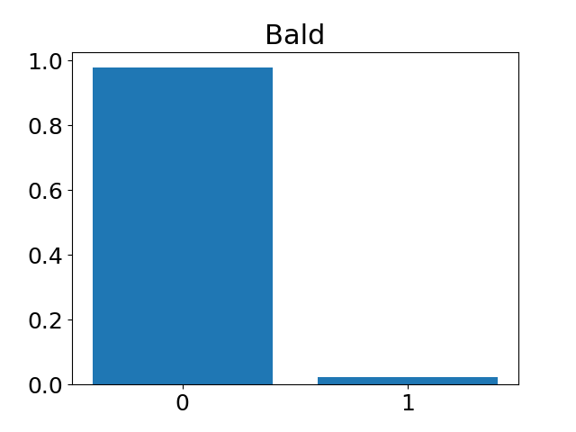
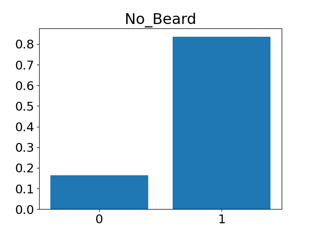
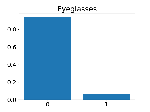
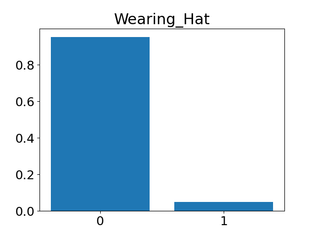
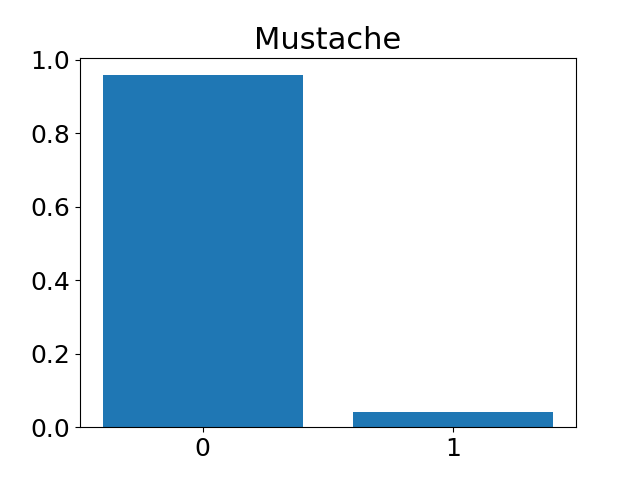
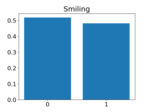
Figure 6: Distributions of the attributes bald, beard, eyeglasses, hat, mustache, and smiling in the CelebA dataset.

C.2 Details about Datasets

Adult Income dataset (Dua and Graff, 2017)

The Adult Income dataset is available on the UCI repository (Dua and Graff, 2017). Each record comprises 14 features (before one-hot encoding categorical ones) for an individual, such as their education or marital status, and the task is to predict whether an individual makes more than $50k per year or not (distribution: 23.9% yes - 76.1% no). In Section 5.1, we used the dataset as provided by Lee et al. (2022). They removed the features “fnlwgt” and “race”, and they subsampled the dataset to comprise 2261 records (cf. Appendix I.3 in their paper). They used the binary feature “sex” as demographic attribute (distribution: 66.8% male - 33.2% female). In our comparison with the method of Agarwal et al. (2018) presented in Section 5.2, we also used “sex” as demographic attribute; however, we did not remove any features and we randomly subsampled the dataset to comprise 5000 records for training and 5000 different records for evaluation (i.e., computing a classifier’s accuracy and fairness violation). In the runtime comparison of Appendix C.7 we used between 1000 and 40000 randomly sampled records for training.

Bank Marketing dataset (Moro et al., 2014; Dua and Graff, 2017)

The Bank Marketing dataset is available on the UCI repository (Dua and Graff, 2017). There are four versions available. We worked with the file bank-additional-full.csv. Each record comprises 20 features (before one-hot encoding categorical ones) for an individual, and the task is to predict whether an individual subscribes a term deposit or not (distribution: 11.3% yes - 88.7% no). We used a person’s binarized age (older than 40 vs. not older than 40) as demographic attribute (distribution: 42.3% older than 40 - 57.7% not older than 40), and we randomly subsampled the dataset to comprise 5000 records for training and 5000 different records for evaluation.

CelebA dataset (Liu et al., 2015)

The CelebA dataset comprises 202599 pictures of faces of celebrities together with 40 binary attribute annotations for each picture. The dataset comes in two versions: one that provides in-the-wild images, which may not only show a person’s face, but also their upper body, and one that provides aligned-and-cropped images, which only show a person’s face. For our experiment, we used the latter one. We used one of the bald, beard, eyeglasses, hat, mustache, or smiling annotations as demographic attributes. The distributions of these attributes can be seen in Figure 6.

COMPAS dataset (Angwin et al., 2016)

The COMPAS dataset is available on https://github.com/propublica/compas-analysis. We used the dataset as provided by Lee et al. (2022). They subsampled the dataset to comprise 2468 datapoints, removed the features “sex” and “c_charge_desc”, and used the feature “Race” for defining the demographic attribute (cf. Appendix I.1 in their paper).

German Credit (Dua and Graff, 2017)

The German Credit dataset is available on the UCI repository (Dua and Graff, 2017). It comprises 1000 datapoints. We used the dataset as provided by Lee et al. (2022). They removed the features “sex” and “personal_status” and used the feature “Age” for defining the demographic attribute (cf. Appendix I.2 in their paper).

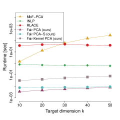
Figure 7: The running time of MbF-PCA (Lee et al., 2022), INLP (Ravfogel et al., 2020), RLACE (Ravfogel et al., 2022) and our proposed methods as a function of the target dimension $k$. The data dimension $d$ equals 100. Note the logarithmic y-axis.

C.3 Another Runtime Comparison

Figure 7 provides a comparison of the running times of the various methods (except for FPCA, which we already have seen to run extremely slow in Figure 4) in a related, but different setting as in the experiments of Section 5.1 on the synthetic data. The data is generated in the same way as in Section 5.1, but now we vary the target dimension $k$ and hold the data dimension $d$ constant at 100. We see that while the running time of our proposed methods only moderately increases with $k$, the running time of MbF-PCA drastically increases with $k$. Note that the running time of INLP even decreases with $k$, which is by the design of the method (cf. Section 4).

C.4 Tables for German Credit and COMPAS

Table 2 and Table 3 provide the results of the experiments of Section 5.1 on the real data for the German Credit dataset and the COMPAS dataset, respectively. Note that the dimension of the COMPAS dataset is rather small—in particular, for $k=10$, we do not expect Fair PCA-S (0.5) or Fair PCA-S (0.85) to behave any differently than fair PCA since $l=\max\{k,\lfloor f\cdot d\rfloor\}=k=d-1$ for both $f=0.5$ and $f=0.85$.

Table 2: Similar table as Table 1 for the German Credit dataset.

German Credit [$\text{feature dim}=57$, $\operatorname{Pr}(Y=1)=0.3020$]
$k$	Algorithm	%Var($\uparrow$)	MMD2($\downarrow$)	%Acc($\uparrow$)	$\Delta_{DP}$($\downarrow$)	%Acc($\uparrow$)	$\Delta_{DP}$($\downarrow$)	%Acc($\uparrow$)	$\Delta_{DP}$($\downarrow$)
				Kernel SVM		Linear SVM		MLP
2	PCA	$\mathbf{11.42_{0.45}}$	$\mathbf{0.147_{0.047}}$	$\mathbf{76.87_{1.32}}$	$\mathbf{0.12_{0.06}}$	$\mathbf{69.8_{1.21}}$	$\mathbf{0.0_{0.0}}$	$\mathbf{71.7_{1.83}}$	$\mathbf{0.09_{0.09}}$
2-10	FPCA (0.1, 0.01)	$7.43_{0.56}$	$0.017_{0.009}$	$72.17_{1.04}$	$0.03_{0.02}$	$\mathbf{69.8_{1.21}}$	$\mathbf{0.0_{0.0}}$	$70.27_{1.38}$	$0.01_{0.01}$
	FPCA (0, 0.01)	$7.33_{0.54}$	$0.015_{0.01}$	$71.77_{1.52}$	$0.03_{0.02}$	$\mathbf{69.8_{1.21}}$	$\mathbf{0.0_{0.0}}$	$69.83_{1.49}$	$\mathbf{0.0_{0.01}}$
	MbF-PCA ($10^{-3}$)	$\mathbf{10.34_{0.57}}$	$0.019_{0.014}$	$\mathbf{74.87_{1.92}}$	$0.04_{0.04}$	$\mathbf{69.8_{1.21}}$	$\mathbf{0.0_{0.0}}$	$\mathbf{71.43_{2.08}}$	$0.04_{0.05}$
	MbF-PCA ($10^{-6}$)	$9.38_{0.3}$	$0.016_{0.009}$	$73.97_{1.59}$	$0.03_{0.02}$	$\mathbf{69.8_{1.21}}$	$\mathbf{0.0_{0.0}}$	$70.83_{1.66}$	$0.03_{0.03}$
	INLP	$2.99_{0.39}$	$\mathbf{0.007_{0.004}}$	$70.93_{1.27}$	$\mathbf{0.02_{0.02}}$	$\mathbf{69.8_{1.21}}$	$\mathbf{0.0_{0.0}}$	$70.17_{1.56}$	$0.01_{0.02}$
	RLACE	$3.62_{0.27}$	$0.042_{0.027}$	$71.5_{1.75}$	$\mathbf{0.02_{0.02}}$	$\mathbf{69.8_{1.21}}$	$\mathbf{0.0_{0.0}}$	$70.23_{1.5}$	$0.02_{0.01}$
2-10	Fair PCA	$\mathbf{10.85_{0.55}}$	$0.025_{0.016}$	$\mathbf{75.6_{1.89}}$	$0.06_{0.05}$	$\mathbf{69.8_{1.21}}$	$\mathbf{0.0_{0.0}}$	$\mathbf{72.03_{1.98}}$	$0.04_{0.05}$
	Fair Kernel PCA	$n/a$	$n/a$	$69.8_{1.21}$	$\mathbf{0.0_{0.0}}$	$\mathbf{69.8_{1.21}}$	$\mathbf{0.0_{0.0}}$	$69.8_{1.21}$	$\mathbf{0.0_{0.0}}$
	Fair PCA-S (0.5)	$4.73_{0.43}$	$\mathbf{0.01_{0.006}}$	$72.47_{3.14}$	$0.02_{0.02}$	$\mathbf{69.8_{1.21}}$	$\mathbf{0.0_{0.0}}$	$70.93_{2.21}$	$0.01_{0.01}$
	Fair PCA-S (0.85)	$7.43_{0.42}$	$0.018_{0.011}$	$72.93_{2.05}$	$0.02_{0.02}$	$\mathbf{69.8_{1.21}}$	$\mathbf{0.0_{0.0}}$	$70.0_{1.83}$	$0.02_{0.02}$
10	PCA	$\mathbf{38.24_{0.92}}$	$\mathbf{0.13_{0.018}}$	$\mathbf{99.93_{0.13}}$	$\mathbf{0.12_{0.07}}$	$\mathbf{74.8_{1.93}}$	$\mathbf{0.15_{0.11}}$	$\mathbf{96.87_{2.08}}$	$\mathbf{0.11_{0.08}}$
2-10	FPCA (0.1, 0.01)	$29.85_{0.82}$	$0.02_{0.005}$	$\mathbf{99.93_{0.13}}$	$0.12_{0.07}$	$71.13_{2.75}$	$0.02_{0.03}$	$\mathbf{96.77_{1.8}}$	$0.1_{0.07}$
	FPCA (0, 0.01)	$29.74_{0.84}$	$0.02_{0.005}$	$\mathbf{99.93_{0.13}}$	$0.12_{0.07}$	$70.87_{2.38}$	$0.02_{0.04}$	$96.4_{1.77}$	$0.1_{0.07}$
	MbF-PCA ($10^{-3}$)	$\mathbf{34.07_{1.0}}$	$0.019_{0.007}$	$\mathbf{99.93_{0.13}}$	$0.12_{0.07}$	$\mathbf{73.7_{2.58}}$	$0.05_{0.04}$	$96.67_{1.04}$	$0.11_{0.06}$
	MbF-PCA ($10^{-6}$)	$16.82_{1.11}$	$\mathbf{0.011_{0.007}}$	$94.37_{2.63}$	$0.12_{0.06}$	$70.1_{0.63}$	$\mathbf{0.0_{0.0}}$	$80.07_{3.52}$	$\mathbf{0.06_{0.05}}$
	INLP	$15.5_{0.92}$	$\mathbf{0.011_{0.002}}$	$98.83_{0.79}$	$\mathbf{0.11_{0.07}}$	$69.8_{1.21}$	$\mathbf{0.0_{0.0}}$	$94.2_{2.26}$	$0.1_{0.06}$
	RLACE	$17.24_{0.75}$	$0.03_{0.023}$	$99.73_{0.29}$	$0.12_{0.07}$	$70.97_{2.31}$	$0.02_{0.03}$	$95.43_{2.89}$	$0.12_{0.07}$
2-10	Fair PCA	$\mathbf{36.63_{1.04}}$	$0.022_{0.008}$	$\mathbf{99.93_{0.13}}$	$0.12_{0.07}$	$\mathbf{74.1_{2.23}}$	$0.05_{0.04}$	$96.03_{2.26}$	$0.11_{0.04}$
	Fair Kernel PCA	$n/a$	$n/a$	$70.1_{1.18}$	$\mathbf{0.0_{0.01}}$	$69.8_{1.21}$	$\mathbf{0.0_{0.0}}$	$74.07_{2.43}$	$\mathbf{0.06_{0.03}}$
	Fair PCA-S (0.5)	$20.51_{0.79}$	$\mathbf{0.013_{0.006}}$	$99.87_{0.22}$	$0.12_{0.08}$	$71.6_{2.83}$	$0.02_{0.04}$	$95.13_{2.52}$	$0.08_{0.06}$
	Fair PCA-S (0.85)	$28.83_{0.82}$	$0.018_{0.007}$	$\mathbf{99.93_{0.13}}$	$0.12_{0.07}$	$71.87_{2.62}$	$0.03_{0.04}$	$\mathbf{96.27_{2.0}}$	$0.09_{0.07}$

Table 3: Similar table as Table 1 for the COMPAS dataset.

COMPAS [$\text{feature dim}=11$, $\operatorname{Pr}(Y=1)=0.4548$]
$k$	Algorithm	%Var($\uparrow$)	MMD2($\downarrow$)	%Acc($\uparrow$)	$\Delta_{DP}$($\downarrow$)	%Acc($\uparrow$)	$\Delta_{DP}$($\downarrow$)	%Acc($\uparrow$)	$\Delta_{DP}$($\downarrow$)
				Kernel SVM		Linear SVM		MLP
2	PCA	$\mathbf{39.28_{4.91}}$	$\mathbf{0.092_{0.009}}$	$\mathbf{64.53_{1.38}}$	$\mathbf{0.29_{0.08}}$	$\mathbf{56.69_{1.52}}$	$\mathbf{0.2_{0.09}}$	$\mathbf{61.77_{2.81}}$	$\mathbf{0.28_{0.06}}$
2-10	FPCA (0.1, 0.01)	$\mathbf{35.06_{4.9}}$	$0.012_{0.007}$	$61.65_{1.11}$	$0.1_{0.06}$	$56.23_{1.19}$	$0.04_{0.03}$	$57.61_{1.67}$	$0.08_{0.04}$
	FPCA (0, 0.01)	$34.43_{4.76}$	$0.011_{0.006}$	$60.86_{1.03}$	$0.11_{0.06}$	$55.9_{1.26}$	$0.03_{0.03}$	$56.9_{1.88}$	$0.09_{0.03}$
	MbF-PCA ($10^{-3}$)	$34.24_{3.68}$	$0.006_{0.003}$	$\mathbf{64.78_{0.96}}$	$0.12_{0.05}$	$56.92_{2.7}$	$0.07_{0.06}$	$\mathbf{60.53_{1.46}}$	$0.1_{0.06}$
	MbF-PCA ($10^{-6}$)	$13.52_{2.76}$	$0.002_{0.002}$	$58.26_{1.29}$	$0.03_{0.02}$	$55.01_{0.9}$	$0.01_{0.03}$	$56.15_{1.52}$	$0.04_{0.04}$
	INLP	$0.42_{1.25}$	$\mathbf{0.0_{0.0}}$	$54.95_{1.51}$	$\mathbf{0.01_{0.02}}$	$54.52_{0.7}$	$\mathbf{0.0_{0.0}}$	$54.95_{1.51}$	$\mathbf{0.01_{0.02}}$
	RLACE	$19.18_{4.03}$	$0.008_{0.007}$	$63.36_{1.96}$	$0.1_{0.06}$	$\mathbf{59.64_{3.04}}$	$0.06_{0.05}$	$62.16_{2.67}$	$0.07_{0.04}$
2-10	Fair PCA	$\mathbf{35.56_{4.52}}$	$0.019_{0.007}$	$62.82_{0.88}$	$0.11_{0.08}$	$54.55_{0.76}$	$0.03_{0.04}$	$60.65_{2.29}$	$0.13_{0.11}$
	Fair Kernel PCA	$n/a$	$n/a$	$57.8_{1.82}$	$\mathbf{0.08_{0.06}}$	$54.74_{1.21}$	$\mathbf{0.02_{0.04}}$	$57.67_{1.57}$	$\mathbf{0.05_{0.04}}$
	Fair PCA-S (0.5)	$25.11_{5.14}$	$\mathbf{0.006_{0.004}}$	$\mathbf{64.1_{1.49}}$	$0.15_{0.06}$	$\mathbf{58.08_{2.92}}$	$0.07_{0.05}$	$\mathbf{62.65_{1.75}}$	$0.14_{0.07}$
	Fair PCA-S (0.85)	$35.42_{4.49}$	$0.027_{0.005}$	$60.93_{0.6}$	$0.14_{0.04}$	$55.43_{0.94}$	$0.06_{0.08}$	$56.63_{1.09}$	$0.2_{0.1}$
10	PCA	$\mathbf{100.0_{0.0}}$	$\mathbf{0.241_{0.005}}$	$\mathbf{73.14_{1.16}}$	$\mathbf{0.21_{0.06}}$	$\mathbf{64.78_{0.99}}$	$\mathbf{0.18_{0.05}}$	$\mathbf{69.81_{1.8}}$	$\mathbf{0.23_{0.08}}$
2-10	FPCA (0.1, 0.01)	$87.79_{1.21}$	$0.015_{0.003}$	$72.25_{0.88}$	$\mathbf{0.16_{0.06}}$	$64.7_{1.67}$	$0.06_{0.05}$	$\mathbf{69.73_{1.95}}$	$0.15_{0.07}$
	FPCA (0, 0.01)	$87.44_{1.28}$	$0.015_{0.002}$	$\mathbf{72.32_{0.88}}$	$\mathbf{0.16_{0.07}}$	$64.82_{1.64}$	$\mathbf{0.05_{0.04}}$	$68.52_{1.25}$	$0.08_{0.07}$
	MbF-PCA ($10^{-3}$)	$87.75_{1.29}$	$\mathbf{0.013_{0.002}}$	$72.19_{0.88}$	$\mathbf{0.16_{0.06}}$	$64.97_{1.53}$	$0.08_{0.04}$	$68.89_{1.61}$	$0.11_{0.06}$
	MbF-PCA ($10^{-6}$)	$87.75_{1.29}$	$\mathbf{0.013_{0.002}}$	$72.19_{0.88}$	$\mathbf{0.16_{0.06}}$	$\mathbf{65.01_{1.49}}$	$0.08_{0.04}$	$68.14_{1.14}$	$\mathbf{0.07_{0.05}}$
	INLP	$\mathbf{91.09_{0.88}}$	$0.034_{0.005}$	$71.4_{0.9}$	$0.17_{0.03}$	$64.93_{0.84}$	$0.18_{0.04}$	$68.19_{1.46}$	$0.2_{0.04}$
	RLACE	$87.47_{1.27}$	$0.015_{0.002}$	$72.29_{0.85}$	$\mathbf{0.16_{0.06}}$	$64.75_{1.73}$	$\mathbf{0.05_{0.03}}$	$68.3_{2.07}$	$0.1_{0.07}$
2-10	Fair PCA	$\mathbf{87.44_{1.28}}$	$\mathbf{0.015_{0.002}}$	$\mathbf{72.32_{0.9}}$	$\mathbf{0.16_{0.06}}$	$64.72_{1.69}$	$\mathbf{0.05_{0.03}}$	$67.94_{1.43}$	$\mathbf{0.09_{0.07}}$
	Fair Kernel PCA	$n/a$	$n/a$	$65.96_{1.12}$	$0.26_{0.07}$	$64.33_{0.8}$	$\mathbf{0.05_{0.04}}$	$66.41_{1.03}$	$0.14_{0.07}$
	Fair PCA-S (0.5)	$\mathbf{87.44_{1.28}}$	$\mathbf{0.015_{0.002}}$	$72.31_{0.88}$	$\mathbf{0.16_{0.06}}$	$\mathbf{64.75_{1.7}}$	$\mathbf{0.05_{0.03}}$	$\mathbf{69.24_{2.02}}$	$0.12_{0.06}$
	Fair PCA-S (0.85)	$\mathbf{87.44_{1.28}}$	$\mathbf{0.015_{0.002}}$	$72.31_{0.88}$	$\mathbf{0.16_{0.06}}$	$\mathbf{64.75_{1.7}}$	$\mathbf{0.05_{0.03}}$	$\mathbf{69.24_{2.02}}$	$0.12_{0.06}$

Table 4: We applied the fair PCA method of Samadi et al. (2018) to the three real-world datasets considered in Section 5.1. The tables do not provide the metrics %Var and MMD² since the method of Samadi et al. is not guaranteed to yield an embedding of the desired target dimension, and hence their method and the methods studied in Section 5.1 are not comparable w.r.t. %Var and MMD².

Adult Income [$\text{feature dim}=97$, $\operatorname{Pr}(Y=1)=0.2489$]
$k$	Algorithm	%Acc($\uparrow$)	$\Delta_{DP}$($\downarrow$)	%Acc($\uparrow$)	$\Delta_{DP}$($\downarrow$)	%Acc($\uparrow$)	$\Delta_{DP}$($\downarrow$)
		Kernel SVM		Linear SVM		MLP
2	Fair PCA of Samadi et al. (2018)	$81.59_{1.12}$	$0.14_{0.03}$	$80.8_{1.09}$	$0.13_{0.04}$	$82.02_{1.03}$	$0.18_{0.04}$
10	Fair PCA of Samadi et al. (2018)	$87.78_{0.87}$	$0.18_{0.02}$	$83.2_{1.09}$	$0.13_{0.03}$	$91.34_{2.04}$	$0.18_{0.03}$
German Credit [$\text{feature dim}=57$, $\operatorname{Pr}(Y=1)=0.3020$]
$k$	Algorithm	%Acc($\uparrow$)	$\Delta_{DP}$($\downarrow$)	%Acc($\uparrow$)	$\Delta_{DP}$($\downarrow$)	%Acc($\uparrow$)	$\Delta_{DP}$($\downarrow$)
		Kernel SVM		Linear SVM		MLP
2	Fair PCA of Samadi et al. (2018)	$73.73_{1.38}$	$0.05_{0.03}$	$69.97_{0.82}$	$0.0_{0.01}$	$72.97_{1.4}$	$0.04_{0.02}$
10	Fair PCA of Samadi et al. (2018)	$98.73_{0.7}$	$0.1_{0.07}$	$76.8_{1.9}$	$0.09_{0.07}$	$98.13_{0.69}$	$0.12_{0.07}$
COMPAS [$\text{feature dim}=11$, $\operatorname{Pr}(Y=1)=0.4548$]
$k$	Algorithm	%Acc($\uparrow$)	$\Delta_{DP}$($\downarrow$)	%Acc($\uparrow$)	$\Delta_{DP}$($\downarrow$)	%Acc($\uparrow$)	$\Delta_{DP}$($\downarrow$)
		Kernel SVM		Linear SVM		MLP
2	Fair PCA of Samadi et al. (2018)	$63.89_{1.86}$	$0.2_{0.05}$	$57.94_{2.22}$	$0.12_{0.05}$	$63.95_{3.98}$	$0.18_{0.03}$
10	Fair PCA of Samadi et al. (2018)	$73.12_{1.17}$	$0.21_{0.06}$	$64.79_{0.96}$	$0.18_{0.05}$	$69.46_{1.04}$	$0.27_{0.09}$

C.5 Comparison with Samadi et al. (2018)

We applied the fair PCA method of Samadi et al. (2018) to the three real-world datasets considered in Section 5.1. As discussed in Section 4 and Section 5.1, the fairness notion underlying the method of Samadi et al. is incomparable to our notion of fair PCA. Samadi et al. provide theoretical guarantees for an algorithm that relies on solving a semidefinite program (SDP), but then propose to use a multiplicative weight update method for solving the SDP approximately in order to speed up computation. We observed that this can result in embedding dimensions that are much larger than the desired target dimension. We used the code provided by Samadi et al. without modifications; in particular, we used the same parameters for the multiplicative weight update algorithm as they used in their experiment on the LFW dataset.

Table 4 provides the results. We see that the downstream classifiers trained on the fair PCA representation of Samadi et al. have roughly similar values of accuracy and DP violation as standard PCA. Clearly, the DP violations are much higher than for our methods or the other competitors. Since the dimension of the fair PCA representation of Samadi et al. is not guaranteed to equal the desired target dimension $k$, we do not report the metrics %Var and MMD² in Table 4.

C.6 Fair PCA Applied to the CelebA Dataset

Figures 10 to 15 show examples of original CelebA images (top row of each figure) together with the results of applying fair PCA (middle and bottom row) for the various demographic attributes. We see that fair PCA adds something looking like glasses / a mustache / a beard to the faces, making it hard to tell whether an original face features those, and successfully obfuscates the demographic information for these attributes. Still the projected faces resemble the original ones to a good extent. For the attribute “smiling”, fair PCA also succeeds in obfuscating the demographic information, but the whole faces become more perturbed and less similar to the original ones. For the attributes “bald” and “hat”, fair PCA appears to fail, and we can tell for all of the faces under consideration that they do not feature baldness / a hat. We suspect that the reason for this might be the high diversity of hats or non-bald faces (see Figure 16 for some example images).

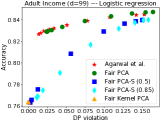
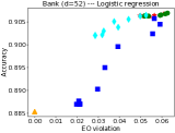
Figure 8: Comparison with the state-of-the-art reductions approach of Agarwal et al. (2018) when training a logistic regression classifier on the Adult Income dataset (first and second plot) and the Bank Marketing dataset (third and fourth plot). Compared to the plots in Figure 4, these plots also show the results for Fair PCA-S and fair kernel PCA.

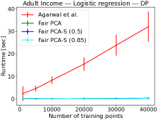
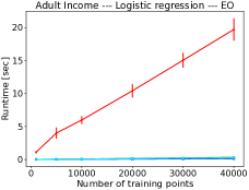
Figure 9: Runtime comparison between our methods and the method of Agarwal et al. (2018). For our methods, the running time includes the time it takes to fit the logistic regression classifier on top of the fair representation.

C.7 Comparison with Agarwal et al. (2018)

Figure 8 shows the results of the comparison with the reductions approach of Agarwal et al. (2018) when training a logistic regression classifier for Fair PCA-S and fair kernel PCA (next to the results for fair PCA and the method of Agarwal et al., which we have already seen in Figure 4 in Section 5.2). We see that Fair PCA-S produces smooth trade-off curves and can achieve lower fairness violation than fair PCA or the method of Agarwal et al. in some cases. However, the representation learned by fair kernel PCA only allows for a constant logistic regression classifier (with zero fairness violation and an accuracy equaling the probability of the predominant label—cf. Appendix C.2).

The plots of Figure 9 show the running time of the various methods as a function of the number of training points on the Adult Income dataset and when training a logistic regression classifier. The curves show the average over the eleven values of the fairness parameter / the parameter difference_bound (cf. Appendix C.1) and over ten random draws of training data together with the standard deviation as error bars. Note that for our methods the running time includes the time it takes to train the classifier on a representation produced by our method. While none of our methods ever runs for more than 0.5 seconds, the method of Agarwal et al., on average, runs for more than 32 seconds when training with 40000 datapoints and aiming for DP. The plots do not show curves for fair kernel PCA, which we cannot simply apply to this large number of training points due to its cubic running time in the number of datapoints. We leave it as an interesting question for future work to develop scalable approximation techniques for fair kernel PCA similarly to those that have been developed for standard kernel PCA or other kernel methods (e.g., Williams and Seeger, 2000; Kim et al., 2005; Chin and Suter, 2006).

Original

dim$=$6400

 

Fair PCA

$k=6399$

Fair PCA

$k=400$

Figure 10: Fair PCA applied to the CelebA dataset to erase the concept of “glasses”.

Original

dim$=$6400

 

Fair PCA

$k=6399$

Fair PCA

$k=400$

Figure 11: Fair PCA applied to the CelebA dataset to erase the concept of “mustache”.

Original

dim$=$6400

 

Fair PCA

$k=6399$

Fair PCA

$k=400$

Figure 12: Fair PCA applied to the CelebA dataset to erase the concept of “beard”.

Original

dim$=$6400

 

Fair PCA

$k=6399$

Fair PCA

$k=400$

Figure 13: Fair PCA applied to the CelebA dataset to erase the concept of “smiling”.

Original

dim$=$6400

 

Fair PCA

$k=6399$

Fair PCA

$k=400$

Figure 14: Fair PCA applied to the CelebA dataset to erase the concept of “bald”.

Original

dim$=$6400

 

Fair PCA

$k=6399$

Fair PCA

$k=400$

Figure 15: Fair PCA applied to the CelebA dataset to erase the concept of “hat”.

Figure 16: Examples of faces in the CelebA dataset that feature a hat (top row) or baldness (bottom row). We can see that the hats are highly diverse. Note that both types of faces are rare in the dataset: only 4.8% of the faces feature a hat, and only 2.2% feature baldness (cf. Figure 6).

References

• Adel et al. (2019) T. Adel, I. Valera, Z. Ghahramani, and A. Weller. One-network adversarial fairness. In AAAI Conference on Artificial Intelligence, 2019.
• Agarwal et al. (2018) A. Agarwal, A. Beygelzimer, M. Dudik, J. Langford, and H. Wallach. A reductions approach to fair classification. In International Conference on Machine Learning (ICML), 2018. Implemented in Fairlearn: https://fairlearn.org/.
• Alvi et al. (2019) M. Alvi, A. Zisserman, and C. Nellaker. Turning a blind eye: Explicit removal of biases and variation from deep neural network embeddings. In European Conference on Computer Vision (ECCV) - Workshop, 2019.
• Angwin et al. (2016) J. Angwin, J. Larson, S. Mattu, and L. Kirchner. Propublica—machine bias, 2016. https://www.propublica.org/article/machine-bias-risk-assessments-in-criminal-sentencing.
• Balunovic et al. (2022) M. Balunovic, A. Ruoss, and M. Vechev. Fair normalizing flows. In International Conference on Learning Representations (ICLR), 2022.
• Barocas et al. (2018) S. Barocas, M. Hardt, and A. Narayanan. Fairness and Machine Learning. fairmlbook.org, 2018. http://www.fairmlbook.org.
• Beutel et al. (2017) A. Beutel, J. Chen, Z. Zhao, and E. Chi. Data decisions and theoretical implications when adversarially learning fair representations. arXiv:1707.00075 [cs.LG], 2017.
• Chechik et al. (2005) G. Chechik, A. Globerson, N. Tishby, and Y. Weiss. Information bottleneck for Gaussian variables. Journal of Machine Learning Research (JMLR), 6:165–188, 2005.
• Chierichetti et al. (2017) F. Chierichetti, R. Kumar, S. Lattanzi, and S. Vassilvitskii. Fair clustering through fairlets. In Neural Information Processing Systems (NeurIPS), 2017.
• Chin and Suter (2006) T.-J. Chin and D. Suter. Improving the speed of kernel PCA on large scale datasets. In IEEE International Conference on Video and Signal Based Surveillance, 2006.
• Cotter et al. (2019) A. Cotter, H. Narasimhan, and M. Gupta. On making stochastic classifiers deterministic. In Neural Information Processing Systems (NeurIPS), 2019.
• d’Alessandro et al. (2017) B. d’Alessandro, C. O’Neil, and T. LaGatta. Conscientious classification: A data scientist’s guide to discrimination-aware classification. Big Data, 5(2):120–134, 2017.
• Dua and Graff (2017) D. Dua and C. Graff. UCI machine learning repository, 2017. URL http://archive.ics.uci.edu/ml.
• Edwards and Storkey (2016) H. Edwards and A. Storkey. Censoring representations with an adversary. In International Conference on Learning Representations (ICLR), 2016.
• Feng et al. (2019) R. Feng, Y. Yang, Y. Lyu, C. Tan, Y. Sun, and C. Wang. Learning fair representations via an adversarial framework. arXiv:1904.13341 [cs.LG], 2019.
• Ghojogh et al. (2019) B. Ghojogh, F. Karray, and M. Crowley. Eigenvalue and generalized eigenvalue problems: Tutorial. arXiv:1903.11240 [stat.ML], 2019.
• Haghighatkhah et al. (2021) P. Haghighatkhah, W. Meulemans, B. Speckmann, J. Urhausen, and K. Verbeek. Obstructing classification via projection. In International Symposium on Mathematical Foundations of Computer Science, 2021.
• Hardt et al. (2016) M. Hardt, E. Price, and N. Srebro. Equality of opportunity in supervised learning. In Neural Information Processing Systems (NIPS), 2016.
• Jia et al. (2018) S. Jia, T. Lansdall-Welfare, and N. Cristianini. Right for the right reason: Training agnostic networks. In International Symposium on Intelligent Data Analysis, 2018.
• Kamani et al. (2022) M. Kamani, F. Haddadpour, R. Forsati, and M. Mahdavi. Efficient fair principal component analysis. Machine Learning, 2022.
• Kamiran and Calders (2011) F. Kamiran and T. Calders. Data preprocessing techniques for classification without discrimination. Knowledge and Information Systems, 33:1–33, 2011.
• Kim et al. (2005) K. I. Kim, M. Franz, and B. Schölkopf. Iterative kernel principal component analysis for image modeling. IEEE Transactions on Pattern Analysis and Machine Intelligence, 27(9):1351–1366, 2005.
• Koller and Sahami (1996) D. Koller and M. Sahami. Toward optimal feature selection. In International Conference on Machine Learning (ICML), 1996.
• Lee et al. (2022) J. Lee, G. Kim, M. Olfat, M. Hasegawa-Johnson, and C. Yoo. Fast and efficient MMD-based fair PCA via optimization over Stiefel manifold. In AAAI Conference on Artificial Intelligence (AAAI), 2022. Code available on https://github.com/nick-jhlee/fair-manifold-pca.
• Liu et al. (2015) Z. Liu, P. Luo, X. Wang, and X. Tang. Deep learning face attributes in the wild. In International Conference on Computer Vision (ICCV), 2015. Dataset available on https://mmlab.ie.cuhk.edu.hk/projects/CelebA.html.
• Louizos et al. (2016) C. Louizos, K. Swersky, Y. Li, M. Welling, and R. Zemel. The variational fair autoencoder. In International Conference on Learning Representations (ICLR), 2016.
• Madras et al. (2018) D. Madras, E. Creager, T. Pitassi, and R. Zemel. Learning adversarially fair and transferable representations. In International Conference on Machine Learning (ICML), 2018.
• Moro et al. (2014) S. Moro, P. Cortez, and P. Rita. A data-driven approach to predict the success of bank telemarketing. Decision Support Systems, 62:22–31, 2014.
• Moyer et al. (2018) D. Moyer, S. Gao, R. Brekelmans, G. Steeg, and A. Galstyan. Invariant representations without adversarial training. In Conference on Neural Information Processing Systems (NeurIPS), 2018.
• Oh et al. (2022) C. Oh, H. Won, J. So, T. Kim, Y. Kim, H. Choi, and K. Song. Learning fair representation via distributional contrastive disentanglement. In ACM SIGKDD International Conference on Knowledge Discovery & Data Mining (KDD), 2022.
• Olfat and Aswani (2019) M. Olfat and A. Aswani. Convex formulations for fair principal component analysis. In AAAI Conference on Artificial Intelligence (AAAI), 2019.
• Pelegrina et al. (2021) G. Pelegrina, R. Brotto, L. Duarte, R. Attux, and J. Romano. A novel multi-objective-based approach to analyze trade-offs in fair principal component analysis. arXiv:2006.06137 [cs.LG], 2021.
• Raff and Sylvester (2018) E. Raff and J. Sylvester. Gradient reversal against discrimination: A fair neural network learning approach. In IEEE International Conference on Data Science and Advanced Analytics (DSAA), 2018.
• Ravfogel et al. (2020) S. Ravfogel, Y. Elazar, H. Gonen, M. Twiton, and Y. Goldberg. Null it out: Guarding protected attributes by iterative nullspace projection. In Annual Meeting of the Association for Computational Linguistics, 2020. Code available on https://github.com/shauli-ravfogel/nullspace_projection.
• Ravfogel et al. (2022) S. Ravfogel, M. Twiton, Y. Goldberg, and R. Cotterell. Linear adversarial concept erasure. In International Conference on Machine Learning (ICML), 2022. Code available on https://github.com/shauli-ravfogel/rlace-icml.
• Samadi et al. (2018) S. Samadi, U. Tantipongpipat, J. Morgenstern, M. Singh, and S. Vempala. The price of fair PCA: One extra dimension. In Neural Information Processing Systems (NeurIPS), 2018. Code available on https://github.com/samirasamadi/Fair-PCA.
• Sarhan et al. (2020) M. H. Sarhan, N. Navab, A. Eslami, and S. Albarqouni. Fairness by learning orthogonal disentangled representations. In European Conference on Computer Vision (ECCV), 2020.
• Schölkopf et al. (2001) B. Schölkopf, R. Herbrich, and A. J. Smola. A generalized representer theorem. In Annual Conference on Computational Learning Theory (COLT), 2001.
• Schölkopf and Smola (2002) B. Schölkopf and A. Smola. Learning with kernels. MIT Press, 2002.
• Shalev-Shwartz and Ben-David (2014) S. Shalev-Shwartz and S. Ben-David. Understanding machine learning: From theory to algorithms. Cambridge University Press, 2014.
• Shao et al. (2022) S. Shao, Y. Ziser, and S. B. Cohen. Gold doesn’t always glitter: Spectral removal of linear and nonlinear guarded attribute information. arXiv:2203.07893 [cs.CL], 2022.
• Song et al. (2019) J. Song, P. Kalluri, A. Grover, S. Zhao, and S. Ermon. Learning controllable fair representations. Proceedings of Machine Learning Research (PMLR), 89:2164–2173, 2019.
• Tantipongpipat et al. (2019) U. Tantipongpipat, S. Samadi, M. Singh, J. Morgenstern, and S. Vempala. Multi-criteria dimensionality reduction with applications to fairness. In Neural Information Processing Systems (NeurIPS), 2019.
• Tishby et al. (1999) N. Tishby, F. C. Pereira, and W. Bialek. The information bottleneck method. In Allerton Conference on Communication, Control, and Computing, 1999.
• Williams and Seeger (2000) C. Williams and M. Seeger. Using the Nyström method to speed up kernel machines. In Neural Information Processing Systems (NIPS), 2000.
• Xie et al. (2017) Q. Xie, Z. Dai, Y. Du, E. Hovy, and G. Neubig. Controllable invariance through adversarial feature learning. arXiv:1705.11122 [cs.LG], 2017.
• Yu and Liu (2004) L. Yu and H. Liu. Efficient feature selection via analysis of relevance and redundancy. Journal of Machine Learning Research (JMLR), 5:1205–1224, 2004.
• Zafar et al. (2019) M. B. Zafar, I. Valera, M. G. Rodriguez, and K. P. Gummadi. Fairness constraints: A flexible approach for fair classification. Journal of Machine Learning Research (JMLR), 20(75):1–42, 2019.
• Zemel et al. (2013) R. Zemel, Y. Wu, K. Swersky, T. Pitassi, and C. Dwork. Learning fair representations. In International Conference on Machine Learning (ICML), 2013.