Observation of tunable discrete time crystalline phases

Abstract

Discrete time crystals (DTCs) are emergent non-equilibrium phases of periodically driven many-body systems, with potential applications ranging from quantum computing to sensing and metrology. There has been significant recent interest in understanding mechanisms leading to DTC formation and a search for novel DTC phases beyond subharmonic entrainment. Here, we report observation of multiple DTC phases in a nanoelectromechanical system (NEMS) based on coupled graphene and silicon nitride membranes. We confirm the time-crystalline nature of these symmetry broken phases by establishing their many-body characters, long-range time and spatial order, and rigidity against parameter fluctuation or noise. Furthermore, we employ controlled mechanical strain to drive the transitions between phases with different symmetries, thereby mapping the emergent time-crystalline phase diagram. Overall, our work takes a step towards establishing time crystals as a system with complexity rivaling that of solid state crystals.

In “More is different”, Anderson speculated on the possibility of symmetry breaking and emergence of stable collective phases in time, in close analogy with emergent crystalline phases in space [1]. Over last decade, renewed interest in possible temporal symmetry breaking resulted in the discovery of discrete time crystals (DTCs), which are emergent phases of interacting periodically driven systems [2, 3, 4, 5, 6, 7, 8, 9, 10]. In a DTC phase, multiple interacting modes of a driven system settle into a common period that is longer than the drive. Such collective breaking of discrete time translational symmetry results in a dynamical steady state, the DTC phase, that exhibits novel features reminiscent of equilibrium thermodynamic phases. Such phases have been suggested for applications in computation, metrology, and sensing  [11, 12, 13]. Experiments in quantum systems with ions, atoms and defects in solids observed signatures of DTC in the form of subharmonic entrainment [14, 15, 16]. Nevertheless, multiple questions regarding the origin and nature of DTCs remain unanswered. First, what mechanisms ensure stability of DTC phases against drive heating and fluctuations [17, 18]? Second, can a truly many-body DTC phase arise in a fully classical system [17]? Third, are there DTC phases with complex symmetry types beyond subharmonic entrainment [17, 19, 20, 21, 22]?

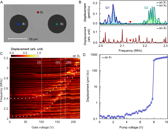
Figure 1: The system: (A) SEM image of the device comprised of two graphene drums (black, the two $20$ $\mu m$ diameter drums are used for all experiments) suspended on a SiNx membrane (gray). Three dots on the sample depict the detection points on graphene ($X_{1}$, $X_{2}$) and SiNx ($X_{3}$) surface (blue, green and red, respectively). (B) Blue and green curves (upper panel) show thermal spectra of the two graphene drums measured at $X_{1}$ and $X_{2}$. The spectrum is described by two Lorentzian peaks due to graphene drums (dotted) hybridized with multiple SiNx modes. These modes are visible directly in a measurement (at $X_{3}$) on SiNx surface (lower panel). (C) Weakly driven spectra of SiNx, measured at $X_{3}$. With varying DC gate voltage (controlling the tension), we observe dispersion of the two graphene modes with tunable frequency separation (white dotted curves). These modes hybridize with different sets of SiNx modes at different frequencies. Three typical phases of Figs. 2B, C and D, are observed at voltages corresponding to (ii), (i) and (iii), respectively. (D) Spectral amplitude at the midpoint ($\omega$, marked red in Fig. 1B) of the two resonators, with increasing amplitude of a parametric drive (AC gate voltage) at a frequency $2\omega$.

Here, we answer some of these questions by observing a range of new DTC phases as well as transitions between them in a classical NEMS. The phases satisfy three accepted criteria of genuine DTCs  [19, 23, 17, 12]:

(1) Interacting many-mode system: We fabricate a device in which multiple mechanical modes of a Silicon Nitride (SiNx) resonator interact with two spatially separated graphene resonators. Moreover, exceptional elastic and mechanical non-linear properties of graphene [24] make the interaction tunable, resulting in long-range interaction between otherwise non-interacting many (on average 16) SiNx modes (see SI, section IV).

(2) Collective breaking of discrete symmetry in time: When driven parametrically at twice of the average frequency of the hybrid modes, universal collective modes emerge sharply above a threshold drive power, breaking discrete time translational symmetry of the drive. In classical dynamical systems, such discrete time translation symmetry breaking is ubiquitous, ranging from parametrically driven swings to Faraday waves [25]. Though in principle such systems are composed of many modes, the symmetry breaking oscillation can nevertheless be described as parametric driving of a single normal mode without any distinct many-mode features  [26, 27, 28, 29]. In contrast, symmetry breaking in weakly coupled many-mode systems at finite temperature and fluctuations, a hall-mark of DTC phases, is non-trivial  [12, 11, 30, 23]. Even with two weakly coupled parametric oscillators, common overlap of dynamical instability regions of the resonator modes has lead to DTC-like features [19]. Remarkably, with many interacting modes we observe enhanced rigidity along with a rich palette of distinct DTC phases that can be distinguished by symmetry types including sub-harmonic, anharmonic and a novel biharmonic phase [15, 14, 16, 31, 32, 33]. Furthermore, the spectra, integrated over millions of oscillation periods and measured at differing spatial locations on the resonator surfaces, show evidence for emergence of long-range order in time and space due to interactions between modes of spatially distinct graphene and SiNx oscillators. We note that these DTC phases cannot be fully described within a mean-field model, as would be the case for a one or few-body system.

(3) Rigidity of DTC phases: In contrast to sensitivity of conventional phase synchronization to external parameters [34, 35], the observed DTC phases are surprisingly stable with respect to a broad range of parameter fluctuations. The rigidity to externally added noise is beyond predictions of effective two-mode mean-field models [36, 33]. With increased noise DTCs eventually melt to a non-crystalline phase, marked by broadened spectra and sharp phase boundary, a recently conjectured telltale signature of genuine many-body DTCs [17].

Analysis of a mean-field model indicate that for DTCs, akin to crystals in space, additional physical constraints lead to new emergent phases and such constraints are dynamical in nature, resulting in novel DTC phases due to bifurcations of fixed points and limit cycles with changing mode coupling and frequency detuning [36, 33, 23].

Device and experiment

The device consists of a large area ($320\times 320$ $\mu$m²) SiNx resonator with atomically thin graphene deposited onto two $20$ $\mu$m holes drilled in its surface, forming a second set of resonators $G_{1}$ and $G_{2}$ (Fig. 1A). The system is driven by applying an AC gate voltage via gate electrode (see SI, section I). For initial characterization, thermal noise or low-power measurements are used. Vibrational spectra are measured with a confocal microscope focused on either of the graphene drums ($X_{1}$ or $X_{2}$ in Fig. 1A) or SiNx ($X_{3}$ in Fig. 1A) [37]. When measured on SiNx, a low inbuilt tension and high quality factor result in individually resolvable but densely packed spectra of modes (Fig. 1B, below). Measurements on graphene reveal lower quality factors fundamental modes of the relevant drums hybridized with multiple SiNx modes (Fig. 1B, above). This hybridization induces effective nonlinear cross-talk between the SiNx modes (Fig. 1B) [38]. With increasing tension in the system, controlled by the DC component of gate voltage, the frequencies of flexible graphene drums up-shift (dotted lines in Fig. 1C) while the modes of rigid SiNx remain virtually unchanged (horizontal lines in Fig. 1C). Nevertheless, G1 and G2 remain spectral decoupled in the entire range of DC gate voltages and interact with differing sets of SiNx modes. No signature of direct interaction (e.g. avoid crossing vs. DC gate voltage [38]) between the two graphene resonators is observed.

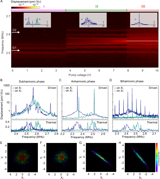
Figure 2: Phases of DTC: (A) Displacement spectra measured at $X_{1}$, corresponding to DC gate voltage (ii), Fig. 1C, with increasing amplitude of a parametric drive at twice of the frequency $\omega$ of the center of the clusters of hybrid modes (inset). Region I exhibits the isolated cluster of hybrid modes corresponding to G1, region II shows a sharp transition to a correlated liquid-like phase while in region III, the system undergoes a transition to a DTC phase. (B) Subharmonic DTC phase observed at gate voltage (ii), Fig. 1C. (C) Anharmonic DTC phase with gate voltage (i), Fig. 1C. (D) Biharmonic DTC phase with gate voltage (iii), Fig. 1C. Lower panels of B-D show corresponding thermal peaks. All measurements carried out at the point $X_{1}$ (blue) and $X_{2}$ (green).(E, F) Quadrature plots ($X_{1}-Y_{1}$ and $X_{2}-Y_{2}$) corresponding to the two peaks of the anharmonic phase (Fig. 2C) show thermal-like fluctuations. (G, H) Cross quadratures ($X_{1}-Y_{2}$ and $X_{2}-Y_{1}$) show strong anti-correlation.

Emergent DTC phases

To access time-crystalline behaviours, the device is parametrically driven at twice of the mean frequency of the clusters of hybrid modes around G1 and G2 (inset, Fig. 2A). With increasing drive strength, the spectral amplitude at $\omega$ first rises from the noise floor at $4$V and then undergoes a sharp transition to a high-amplitude steady state at around $8$V (Fig. 1D). In region I of Fig. 2A, the corresponding spectra contain distinct signatures of graphene-SiNx interactions of the separated clusters of thermal modes around G1 and G2. With increasing drive voltage, the two clusters merge sharply (around 4V, region II) to a single shared spectra, that nevertheless remain thermal-like with small amplitude and without any sharp oscillation frequencies. This suggests that a collective many-body state comprised of multiple modes in remote resonators develops satisfying criterion 1. Eventually, at around 8V, a sharp subharmonic peak, satisfying criterion 2, emerges at frequency $\omega$ with oscillation amplitude that are orders of magnitude higher compared to the thermal modes (region III). The DTC spectra is observed to be global in nature, with similar features measured on resonator surfaces at $X_{1}$, $X_{2}$ (blue and green respectively, in Fig. 2B) and $X_{3}$, in contrast to the local features observed below the threshold (Fig. 1B). Along with long-range order in space, the spectra remain stable for millions of oscillation periods over time scales of seconds.

Tuning the frequency separation of graphene and sets of SiNx with DC gate voltage, we observe two other distinct phases with similar long-range order properties in addition to the subharmonic phase shown in Fig. 2B. These are anharmonic (Fig. 2C) and biharmonic (Fig. 2D) phases, distinguished by even or odd numbers of frequency comb lines in the spectra. The subharmonic, anharmonic, and biharmonic phases manifest different types of time translational symmetry breaking, satisfying the criterion 2 of DTC. Indeed, several recent theoretical works predict the first two of these DTC phases [32, 39, 33]. To the best of our knowledge, the  biharmonic phase is novel. In the remainder of the manuscript, we confirm that assignment of these as time-crystalline phases, map their phase diagram, and explore transitions between them.

It can be noted that the anharmonic DTC phase provides an indirect means of quantifying correlations by noting that the two sharp spectral peaks at frequencies $\omega_{1}$ and $\omega_{2}$ are pinned around the thermal peak clusters corresponding to the two graphene drums G1 and G2 (Fig. 2C). The centers of these drums (points $X_{1}$ and $X_{2}$) are separated by 40 micrometers. Therefore, by comparing the correlation between the peaks at $\omega_{1}$ and $\omega_{2}$, we can gauge the extent of spatial correlations in the system. For a single mode corresponding to either G1 or G2, quadrature fluctuations, measured in frame co-evolving at either of the two peak frequencies, show uncorrelated noise reminiscent of thermal equilibrium (Figs. 2E, F). In striking contrast, cross-correlation measurements between the quadrature of two different modes (effectively probing inter-drum correlations) show strong correlation, with a $24$ $dB$ suppression along a specific phase compared to fluctuations in the orthogonal quadrature (Figs. 2G, H), providing additional evidence of emergent long-range order in higher-order correlations or fluctuations. As expected, this correlation in fluctuations is absent below the DTC threshold and thereby, can be ascribed to it’s emergent long-range order.

A mean-field model

Mean-field models of few coupled modes have been successful in providing insights into dynamical features of DTCs [19, 33]. To investigate the nature of the observed phases further, we thereby model the system as two coupled nonlinear graphene modes (with transverse displacement $x_{1}$ and $x_{2}$) with a common parametric drive and open to a thermal bath with damping and fluctuations. The coarse graining model replaces the zoo of many coupled SiNx modes with a direct coupling between the two otherwise decoupled graphene drums. In effect, the model is represented by two damped Mathieu-Van der Pol-Duffing oscillators with bi-linear coupling between them (see SI, section III and  [38]).

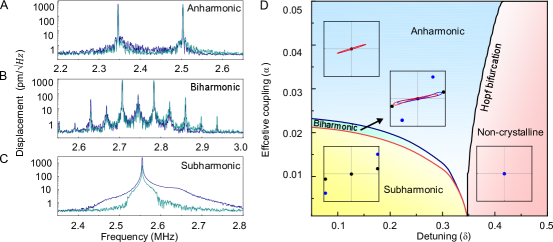
Figure 3: Mean-field phase diagram: Numerical spectrum of the (A) anharmonic phase, (B) biharmonic phase and (C) subharmonic phase like responses (similar to Figs. 2C, D and B respectively) for specific values of parameters, coupling ($\alpha$) , detuning ($\delta$) and drive strength ($h$). (D) Fixed point analysis in parameter space ($\alpha$ vs $\delta$) for $h=0.042$ shows different possible phases of the mean-field model. Red, blue, green and yellow regions are representing non-crystalline, anharmonic, biharmonic and subharmonic responses respectively. Blue and black dots (inset figures corresponding to each region) are stable and unstable fixed points respectively. Elliptical paths around an unstable fixed point represent limit cycles.

Numerical simulations (see SI, section III) indicate the same three DTC phases (subharmonic, anharmonic, and biharmonic; Figs. 3A, B, C) emerging in different parts of the phase diagram (Fig. 3D). This hints that few body classical models at least capture spectral features of genuine many-body DTC phases. A linear stability analysis of the model provides insights into the dynamical nature of the DTC phases. Collective oscillatory DTC phase are mathematically represented as solutions of sinusoidal with frequency $\omega$. Amplitudes of the solutions are slowly varying owing to the weak nonlinearity assumed to facilitate the corresponding rigorous perturbative analyses (see SI, section III). The phases then correspond to robust stable attracting solutions observed for a set of initial conditions of finite measure, while difference in DTC phases manifest as different asymptotic forms of the slowly varying amplitudes. For high enough detuning, stable fixed point, indicating non-crystalline phase (red region, Fig. 3D) appears at the origin (see inset). Reduction in detuning renders this stable solution unstable, eventually yielding limit cycle solutions symmetric about the origin (see inset) via the Hopf bifurcation (black curve, Fig. 3D). The corresponding steady-state oscillations have frequency shifted from $\omega$ resulting in anharmonic DTC phases (blue region, Fig. 3D) [32]. Remarkably, as the coupling strength is further decreased, the limit cycle too loses its stability. However, it bifurcates to give rise to two new stable limit cycles that are not symmetric about origin (see inset), leading to a novel unexplored scenario where DTC spectra bears both the spectral features at frequency $\omega$ as well as the frequencies symmetrically shifted from $\omega$. This suggest a new DTC phase: bi-harmonic (green region, Fig. 3D). The green region indicates existence of more complex solutions that need further detailed analysis. As the coupling strength is further reduced, the two limit cycles eventually disappear leaving only stable fixed points with constant amplitude, shifted away from the origin (see inset). This case corresponds to subharmonic entrainment (yellow region, Fig. 3D) with frequency at $\omega$  [15, 14, 16, 31]. Higher order effects of nonlinearities further complicate the spectra through a series side-peaks in the frequency spectra. Nevertheless, the mean-field model provides crucial insights into the dynamical nature of the DTC phases and dependence to a coarse-grained coupling and mode detuning.

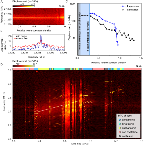
Figure 4: Rigidity of DTC phases: (A) Displacement spectrum density (along Y axis) of subharmonic peak is plotted against noise amplitude (along X axis). (B) Cross section along Y axis of Fig. 4A color map is plotted for minimum (blue) and maximum (red) noise strength. (C) Subharmonic peak amplitude (blue and black curves represent experimental data and numerical results respectively) is plotted against relative noise spectrum density. (D) Experimental observation of displacement spectra at constant DC gate voltage vs parameter pump detuning. The emergent phases characterized by different symmetries are marked above.

Rigidity of DTC phases

Finally, we check the rigidity of the observed phases with respect to noise and parameter fluctuation, the final criterion of the true DTC phase. As an example, to test rigidity against fluctuations, we mix a white noise signal to the drive channel and record the resulting DTC spectra with increasing noise amplitude. Fig. 4A shows a plot of the peak of the subharmonic spectra that remains stable till the relative noise becomes comparable to the drive and eventually melts to a broad noisy spectrum (Fig. 4B). Remarkably, this transition is marked by a sharp phase boundary at specific noise threshold, reminiscent of a first-order thermodynamic phase transition (Fig. 4C, blue). In contrast, numerical simulation of mean field model shows rapid fluctuation between the DTC and a melted phase above a certain noise strength. When averaged over many runs, no sharp transition is observed (Fig. 4C, black). We interpret the stark difference between the experimental system and a mean-field model as a direct evidence for the many body nature of the emergent DTC phase.

The phases are stable in a large frequency window when the drive frequency is detuned. As a function of drive frequency (and at constant tension), we observe broad bands of DTC phases with sharp transitions between them (Fig. 4D). In a remarkably rich phase diagram, we observe additional phases, distinguished by their symmetry, in addition to previously seen subharmonic, anharmonic and biharmonic phases. The continuum phase characterized by a broadband spectrum, requires further investigation and can be a melted, chaotic or a coherent phase. The non-crystalline phase appears for certain pump detuning values which indicates that the drive strength is below threshold. This reflects the dependency of parametric threshold value on pump detuning and coupling of modes. Overall the phase diagram of our hybrid NEMS resonators with transitions between distinct DTC phases rivals the complexity of crystallographic phases of most solid state system.

Outlook

Our results establish existences of truly many-body DTCs in classical systems with distinctly different phases. Observation of rigidity against parameter variations and sharp phase boundaries are found to be emergent many-body features beyond mean-field paradigm. Furthermore, the hybrid NEMS, with exceptional nonlinear and elastic properties of graphene resonators are found to be essential in providing tunable interactions, nonlinearity and damping between many SiNx modes resulting in the stability of the DTC phases.

These results imply multiple directions to explore. Unexplained spectral features (Region II of Fig. 2A and continuum phase of Fig. 4D), can lead to understanding of liquid-like phases in time [21, 9, 8] and the nature of eventual thermalization in these non-equilibrium systems [21, 20]. Correspondence of these DTC phases with their quantum counterparts [20, 21] can lead to insights into interacting quantum systems. For NEMS, multiple graphene resonators in spatially ordered geometries can be extended to new space-time crystalline phases, exceptional spectral rigidity of DTCs can be applied as unique frequency markers in information technology [40, 41, 42] while tunability to phase boundaries can be used in sensors and metrology [43, 44, 45, 46, 47].

Supplementary information: Observation of tunable discrete time crystalline phases

I Materials and Methods

I.1 Device

Low stress silicon-rich silicon nitride is deposited on both sides of a $300\times 300$ $(\mu m)^{2}$ area silicon membrane chip. Array of through holes of $10$, $15$ and $20$ $\mu m$ is patterned on the $300$ $nm$ thick silicon nitride surface. Metallic contact is deposited on the top surface for electrical actuation. High quality chemical vapor deposition (CVD) growth and wet transfer technique is used to make mono layers. Due to Van der Waals force, graphene membranes are clamped on the through holes as a suspended circular drum. The sample is subsequently annealed in an $Ar-H_{2}$ environment at $350^{o}C$.

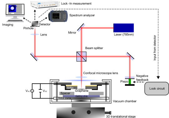
Figure S.1: Experimental setup

I.2 Experimental Setup

Sample is placed in a capacitive arrangement, with a highly doped silicon surface used as a back electrode (see Fig. S.1). DC gate voltage is used to tune the graphene mode frequencies, while AC gate voltage actuates hybrid vibrational modes. The device is kept at room temperature and in vacuum (pressure $\sim 10$ mTorr ). Out of plane motion of the membranes are detected using a confocal microscope, which forms one arm of a Michelson interferometer. To stabilize the signal against external drifts and fluctuations, the two path lengths are actively locked. A frequency and amplitude stabilized external cavity diode laser (ECDL) is used to probe the system. Power of the input signal is kept very low ($\sim 400$ $\mu W$) such that it does not heat up the graphene sample. Detected signal is analyzed with a DAQ for imaging, spectrum analyzer to observe frequency response and a lock-in amplifier for homodyne detection  [37, 38].

II Evidence of correlated fluctuations and long-range order in anharmonic phase

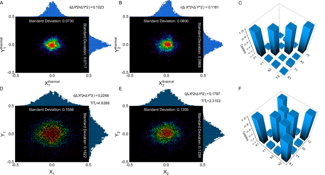
Figure S.2: Correlation: Quadrature plots with histograms of (A) peak at $\omega_{1}$ and (B) peak at $\omega_{2}$ show noise distribution when system is not driven. (C) Plotting covariance matrix we observe no cross-correlation between fundamental mode frequencies when measured on $X_{1}$. (D),(E) and (F) are similar to (A),(B) and (C) respectively when system is driven and showing anharmonic response.

To measure correlation between two spatially separated points on the surface, we study anharmonic response more closely. We have understood earlier that two different peaks of anharmonic response correspond to two different measurement points, one is on graphene drum 1 ($X_{1}$) and the other one is on drum 2 ($X_{2}$). Quadrature measurement using a network analyzer is done to detect fluctuations at $\omega_{1}$ and $\omega_{2}$. We define in phase and out of phase components of peak $\omega_{1}$ and $\omega_{2}$ as $X_{1},Y_{1},X_{2}$ and $Y_{2}$, respectively. When system is not driven, we observe thermal noise distribution (see Fig. S.2A and B ) in phase space due to room temperature.

Furthermore, to quantify the correlation between modes, absolute correlation coefficient is calculated for $X_{1},Y_{1},X_{2},Y_{2}$, defined as [48]

$$C_{i,j}(\tau)=|cov(Z_{i},Z_{j}(\tau))/\sigma_{Z_{i}}\sigma_{Z_{j}}(\tau)|.$$ (S.1)

Here, $cov(Z_{i},Z_{j}(\tau))=\sum_{k}(Z_{i,k}-\bar{Z_{i}})(Z_{j,k}(\tau)-\bar{Z_{j}})/N$, $N$ is total number of data points, $Z_{i}\in\{X_{1},Y_{1},X_{2},Y_{2}\}$ , $\sigma_{Z_{i}}$ is the variance and $\tau$ is time delay between two data points.

Fig. S.2C is showing absolute correlation coefficients at $\tau=0$ correspond to thermal peak. We observe that only auto correlation terms are nonzero because when system is not driven, correlation between quadrature does not exist. When parametric pumping is on, overall fluctuation increases. Looking at $X_{1}$ vs $Y_{1}$ Fig. (S.2D) and $X_{2}$ vs $Y_{2}$ (S.2E) one can conclude that these are same as quadrature of a thermal peak but cross quadrature show anti-correlation (Fig. 2G and H in main text). As a result, we observe non-zero off-diagonal elements of covariance matrix (Fig. S.2F).

Fig. S.3 shows linear variation of correlation coefficients with increasing pump amplitude but with different slope. Covariance $X_{1}-X_{1}$ (red) remains one for all the time when pump strength is increased on the other hand $X_{1}-Y_{1}$ (black) remains zero. $X_{1}-X_{2}$ (navy blue) and $X_{1}-Y_{2}$ (dark cyan) increases with pump amplitude linearly. Navy blue curve saturates around $0.8$ and starts decreasing again.

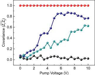
Figure S.3: Variation of covariance with increasing pump amplitude

III Details of the mean-field model

III.1 Effective Hamiltonian of the system

Fig. 1B in main text shows that the fundamental mode of graphene drums can have resonance coupling with many densely packed high quality factor higher order $SiNx$ modes. Here, we have two graphene drums, and both of them are coupled to a few substrate modes on resonance but they are not coupled to each other directly. In a similar fashion, $SiNx$ modes are not directly coupled to each other but coupling exists through graphene modes.

Hamiltonian of this coupled system can be represented as

$$\mathcal{H}=\frac{p_{1}^{2}}{2m_{g}}+\frac{p_{2}^{2}}{2m_{g}}+\sum_{i=3}^{n}\frac{p_{i}^{2}}{2m_{s}}+\frac{1}{2}m_{g}\omega_{1}^{2}x_{1}^{2}+\frac{1}{2}m_{g}\omega_{2}^{2}x_{2}^{2}+\frac{1}{2}m_{s}\sum_{i=3}^{n}\omega_{i}^{2}x_{i}^{2}+\frac{1}{4}\beta(x_{1}^{4}+x_{2}^{4})-\sum_{i=3}^{n}\alpha^{\prime}_{1i}x_{1}x_{i}-\sum_{i=3}^{n}\alpha^{\prime}_{2i}x_{2}x_{i}.$$ (S.2)

We can write following differential equations for this system:

$$\ddot{x}_{1}+\omega_{1}^{2}x_{1}+\frac{\beta}{m_{g}}x_{1}^{3}-\sum_{i=3}^{n}\frac{\alpha^{\prime}_{1i}}{m_{g}}x_{i}=0\,,$$ (S.3a)

$$\ddot{x}_{2}+\omega_{2}^{2}x_{2}+\frac{\beta}{m_{g}}x_{2}^{3}-\sum_{i=3}^{n}\frac{\alpha^{\prime}_{2i}}{m_{g}}x_{i}=0\,,$$ (S.3b)

$$\ddot{x}_{i}+\omega_{i}^{2}x_{i}-\frac{\alpha^{\prime}_{1i}}{m_{s}}x_{1}-\frac{\alpha^{\prime}_{2i}}{m_{s}}x_{2}=0\,,\quad\forall i=\{3,4,\cdots,n\}.$$ (S.3c)

Now, we know that $SiNx$ is much heavier than graphene membrane $(m_{s}\gg m_{g})$. So displacement of graphene drums are order of magnitude larger than $SiNx$. Observing thermal peaks at fundamental frequencies we take ansatz $x_{1}\sim\cos(\omega_{1}t)$ and $x_{2}\sim\cos(\omega_{2}t)$. In this situation, we will focus on $SiNx$ equations. Because secular terms decay down very fast, only coupling terms act as driving forces for this equation, implying $x_{i}\sim A_{i}\cos(\omega_{1}t)+B_{i}\cos(\omega_{2}t)\sim A^{\prime}_{i}x_{1}+B^{\prime}_{i}x_{2}$ ($A_{i}$, $B_{i}$, $A^{\prime}_{i}$, and $B^{\prime}_{i}$ are some slow variables of time) $\quad\forall i=\{3,4,\cdots,n\}$.

If we plug in this into equation S.3 a and b, we can rewrite equations,

$$\ddot{x}_{1}+\omega_{1}^{2}x_{1}+\frac{\beta}{m_{g}}x_{1}^{3}-\frac{\alpha}{m_{g}}x_{2}=0\,,$$ (S.4a)

$$\ddot{x}_{2}+\omega_{2}^{2}x_{2}+\frac{\beta}{m_{g}}x_{2}^{3}-\frac{\alpha}{m_{g}}x_{1}=0\,.$$ (S.4b)

One of the two coupling terms will get absorbed as fundamental frequency correction terms, and finally we can think of an effective coupling between two graphene drums.

We write effective Hamiltonian for the system,

$$\mathcal{H}_{eff}=\frac{p_{1}^{2}}{2m_{g}}+\frac{p_{2}^{2}}{2m_{g}}+\frac{1}{2}m_{g}\omega_{1}^{2}x_{1}^{2}+\frac{1}{2}m_{g}\omega_{2}^{2}x_{2}^{2}+\frac{1}{4}\beta(x_{1}^{4}+x_{2}^{4})-\alpha x_{1}x_{2}.$$ (S.5)

In our experiments, we take $\omega_{1}=\omega_{0}-\Delta/2$ and $\omega_{2}=\omega_{0}+\Delta/2$, and parametrically drive the system with frequency $2\omega_{0}+\Omega_{p}$ such that the Hamiltonian becomes:

$${H}=\frac{p_{1}^{2}}{2m_{g}}+\frac{p_{2}^{2}}{2m_{g}}+\frac{1}{2}m_{g}\left(\omega_{0}-\frac{\Delta}{2}\right)^{2}x_{1}^{2}+\frac{1}{2}h\cos(\left\{2\omega_{0}+\Omega_{p}\right\}t+\chi_{1})x_{1}^{2}$$ (S.6)

$$\phantom{\mathcal{H}=}+\frac{1}{2}m_{g}\left(\omega_{0}+\frac{\Delta}{2}\right)^{2}x_{2}^{2}+\frac{1}{2}h\cos(\left\{2\omega_{0}+\Omega_{p}\right\}t+\chi_{2})x_{2}^{2}+\beta(x_{1}^{4}+x_{2}^{4})-\alpha x_{1}x_{2}.$$

Estimation of coupling value for simulation: Estimation of this effective coupling value will guide us to do numerical calculations. For $h=0$, we will try to solve Eq. (S.4) by solving eigenvalue problem of the following matrix:

$$\begin{bmatrix}\left(\omega_{0}-\frac{\Delta}{2}\right)^{2}&-\frac{\alpha}{m_{g}}\\ -\frac{\alpha}{m_{g}}&\left(\omega_{0}+\frac{\Delta}{2}\right)^{2}\end{bmatrix}.$$ (S.7)

Eigenvalues of this matrix are,

$${\omega^{2}}_{\pm}=\left({\omega_{0}}^{2}+{(\Delta/2)}^{2}\right)\left[1\pm\frac{\omega_{0}^{2}\Delta^{2}+(\alpha/m_{g})}{\left({\omega_{0}}^{2}+{(\Delta/2)}^{2}\right)}\right],$$ (S.8)

or,

$$\delta\omega=\sqrt{\frac{\omega_{0}^{2}\Delta^{2}+(\alpha/m_{g})}{{\omega_{0}}^{2}+{(\Delta/2)}^{2}}},$$ (S.9)

where $\delta\omega=\omega_{+}-\omega_{-}$.

Due to small coupling $\alpha$, we assume that the separation between the peaks at $\omega_{+}$ and $\omega_{-}$ is approximately equal to the detuning $\Delta$, we arrive at

$$\alpha\simeq\frac{m_{g}\Delta^{2}}{2},$$ (S.10)

for $m_{g}\approx{10}^{-15}$ and $\Delta\approx{10}^{5}$ we get $\alpha\approx{10}^{-4}$.

Fine tuning of $\alpha$ can be done by looking at experimental data.

III.2 Numerical integration of stochastic differential equation

As this system is in contact with a thermal bath at the room temperature, we can introduce effective damping and thermal noise $f$ and write coupled second order differential equations:

$$\ddot{x}_{1}+\gamma\dot{x}_{1}+\omega_{1}^{2}x_{1}+\frac{h}{m_{g}}\cos\left\{(\omega_{1}+\omega_{2})t+\chi_{1}\right\}x_{1}+\frac{\eta}{m_{g}}x_{1}^{2}\dot{x}_{1}+\frac{\beta}{m_{g}}x_{1}^{3}-\frac{\alpha}{m_{g}}x_{2}=f_{1}(t),$$ (S.11a)

$$\ddot{x}_{2}+\gamma\dot{x}_{2}+\omega_{2}^{2}x_{2}+\frac{h}{m_{g}}\cos\left\{(\omega_{1}+\omega_{2})t+\chi_{2}\right\}x_{2}+\frac{\eta}{m_{g}}x_{2}^{2}\dot{x}_{2}+\frac{\beta}{m_{g}}x_{2}^{3}-\frac{\alpha}{m_{g}}x_{1}=f_{2}(t).$$ (S.11b)

Any standard ordinary differential equation (ODE) solver will not give correct result due to stochastic terms. Also while checking robustness, another stochastic term will be added to the equation. So we decide to follow Milstein’s algorithm to solve the equations numerically.

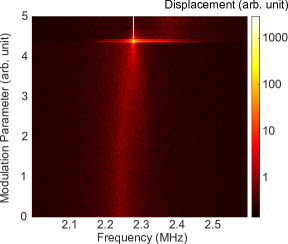
Figure S.4: Subharmonic phase: Simulated spectrum shows appearance of subharmonic phase with increasing modulation parameter and keeping other parameters fixed.

Figure S.5: Anharmonic phase: (A) Anharmonic phase on $X_{1}$ with increasing pump voltage. (B) Numerical result with same conditions on $X_{1}$.

III.2.1 Algorithm to solve stochastic differential equation (SDE)

Let us take a first order differential equation with deterministic and stochastic term  [49]:

$$\frac{dx}{dt}=q(x,t)+g(x,t)\zeta(t),$$ (S.12)

where $q(x,t)$ and $g(x,t)$ are differentiable functions and $\zeta(t)$ is Gaussian white noise ($<\zeta(t)>=0$ and
$<\zeta(t_{1})\zeta(t_{2})>=\delta(t_{1}-t_{2})$).

For $g(x)=0$, this equation becomes an ODE and can be solved using Euler algorithm or RK4.

After a discrete time interval $h$, updated value of $x$ can be expressed as

$$x(t+h)=x(t)+\int_{t}^{t+h}q(x(s),s)ds+\int_{t}^{t+h}g(x(s),s)\zeta(s)ds.$$ (S.13)

Taylor series expansion of functions $q(x,t)$ and $g(x,t)$ give

$$x(t+h)=x(t)+hq(x(t),t)+q^{\prime}(x(t),t)\int_{t}^{t+h}(x(s)-x(t))ds+w_{h}(t)g(x(t),t)$$

$$+g^{\prime}(x(t),t)\int_{t}^{t+h}(x(s)-x(t))\zeta(s)ds+(h+w_{h}(t))\times O[(x(s)-x(t))^{2}],$$ (S.14)

where $w_{h}(t)=\int_{t}^{t+h}\zeta(s)ds$.

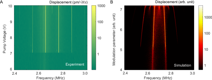
Figure S.6: Biharmonic phase: (A) Experimental observation of biharmonic phase above a threshold value ($9.5V$) of parametric pump voltage and keeping other parameters fixed. (B) Simulated spectrum shows similar behavior.

Incorporating properties of Gaussian noise one can write $w_{h}(t)=\sqrt{h}u(t)$, where $u(t)$ is a set of independent Gaussian random variable with zero mean and variance $1$.

We want to consider all the terms up to first order of h. We can ignore third term of the equation because it is of the order of $h^{2}$. As $w_{h}(t)$ depends on $\sqrt{h}$, we need to evaluate integral of the fourth term. Using Stratonovich calculus we get,

$$g^{\prime}(x(t),t)\int_{t}^{t+h}(x(s)-x(t))\zeta(s)ds=\frac{1}{2}g^{\prime}(x(t),t)g(x(t),t)w^{2}_{h}(t)+O[h^{3/2}].$$ (S.15)

So equation III.2.1 becomes

$$x(t+h)=x(t)+hq(x(t),t)+g(x(t),t)\sqrt{h}u(t)+\frac{h}{2}g(x(t),t)g^{\prime}(x(t),t)u^{2}(t).$$ (S.16)

This recurrence relation is known as the Milshtein algorithm. To use this algorithm for additive noise one have to consider $g(x(t),t)$ is a constant. In that case this relation becomes Euler-Maruyama algorithm:

$$x(t+h)=x(t)+hq(x(t),t)+D\sqrt{h}u(t).$$ (S.17)

Here D is a constant represents additive noise strength.

In equation S.11, thermal fluctuation term is additive, so Euler-Maruyama algorithm will work for us.

III.2.2 Numerical results for DTC phases

We solve equations S.11 using the above mentioned algorithm and we get different spectra for different set of parameter values. Comparing with experimental data, one may conclude that our mean field model is sufficient to explain the time crystalline phases but this results are lacking of essential many body features of the system.

Subharmonic: In experiment, at higher DC gate voltage fundamental modes of graphene drums are close enough to show subharmonic phase when driven parametrically. All the contributing modes start oscillating at half of the pump frequency (Fig. 2A, main text). Above a threshold value ($8V$) of pump voltage we observe subharmonic response. Using equations S.11 with suitable parameters we simulate similar behavior (see Fig. S.4).

Anharmonic: We observe transition from noncrystalline phase to anharmonic phase by changing pump voltage when system is driven at $\omega_{1}+\omega_{2}$. Frequency spectrum (see Fig. S.5A) on $X_{1}$ is recorded. We simulate similar result (Fig. S.5B) using coupled nonlinear equations (S.11).

Biharmonic: We observe transition from noncrystalline phase to anharmonic phase and anharmonic phase to biharmonic phase by changing pump voltage. First transition happens at threshold value $\sim 7V$ and threshold value for biharmonic is $9.5V$. We record frequency spectrum (see Fig. S.6A) and simulate similar result (Fig. S.6B) using coupled nonlinear equations (S.11).

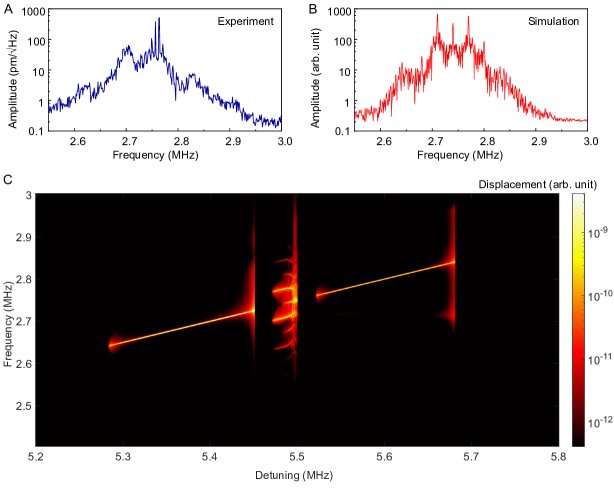
Figure S.7: Continuum: (A) Cross-section of continuum observed in the frequency domain (see Fig. 4D in main text) corresponds to pump frequency value of $5.52$ MHz. (B) Numerical result of two graphene model with an effective coupling shows similar kind of spectrum for pump strength value of 0.0651 (arb. unit) with a $\pi/4$ phase difference between parametric driving signals of the two drums.(C) Numerical observation of different time crystalline phases in the frequency domain for specific values of parameters with detuned pump frequency.

Continuum: Apart from three different time crystalline phases we observe another phase above the parametric pump threshold value which is not discussed in details in this work. For certain parameters, we observe amplification of a wide spectrum around half of the pump frequency (see Fig. S.7A) which we identify as continuum. We observe same feature while simulating our coupled equation for very specific range of parameters (Fig. S.7B). We are still investigating this phase to understand in details.

We study these time crystalline phases experimentally by tuning pump frequency (Fig. 4D in main text). A numerical plot (Fig. S.7C) with two coupled graphene mode shows few features same as Fig. 4D (main text) as also suggestive from Fig. 3 (main text) but experimental data is much more richer than Fig. S.7C due to many-body nature of the system, variation of number of modes, coupling and detuning in experiment.

III.3 Perturbative analysis for a mean-field phase diagram

To understand analytically, we introduce a small book-keeping parameter $\epsilon\equiv 1$ to keep track the order of perturbative equation. We define, $\omega_{0}\equiv\omega-\epsilon\Omega_{p}/2$. Now the model equations take the form,

$$\ddot{x}_{1}+\epsilon\gamma\dot{x}_{1}+\left(\omega-\epsilon\frac{\delta\omega_{1}}{2}\right)^{2}x_{1}+\epsilon\frac{h}{m_{g}}\cos(2\omega t+\chi_{1})x_{1}+\epsilon\frac{\eta}{m_{g}}x_{1}^{2}\dot{x}_{1}+\epsilon\frac{\beta}{m_{g}}x_{1}^{3}-\epsilon\frac{\alpha}{m_{g}}x_{2}=f_{1}(t)$$ (S.18a)

$$\ddot{x}_{2}+\epsilon\gamma\dot{x}_{2}+\left(\omega-\epsilon\frac{\delta\omega_{2}}{2}\right)^{2}x_{2}+\epsilon\frac{h}{m_{g}}\cos(2\omega t+\chi_{2})x_{2}+\epsilon\frac{\eta}{m_{g}}x_{2}^{2}\dot{x}_{2}+\epsilon\frac{\beta}{m_{g}}x_{2}^{3}-\epsilon\frac{\alpha}{m_{g}}x_{1}=f_{2}(t),$$ (S.18b)

where, $\delta\omega_{1}=\Omega_{p}+\Delta$ and $\delta\omega_{2}=\Omega_{p}-\Delta$.

We are now interested in the robust solutions of the above equations. The system is analytically tractable only through perturbative analysis. Considering only the deterministic part, we adopt the multiple time scales method (any equivalent perturbative techniques could be used) and start by writing the ansatz for the equation (S.18a) and equation (S.18b) as,

$$x_{1}(t,T)=x_{1}^{0}(t,T)+\epsilon x_{1}^{1}(t,T)+\cdots$$ (S.19a)

$$x_{2}(t,T)=x_{2}^{0}(t,T)+\epsilon x_{2}^{1}(t,T)+\cdots$$ (S.19b)

As here we have two time scales $t$ and $T\equiv\epsilon t$, therefore

$$\frac{d}{dt}=\frac{\partial}{\partial t}+\epsilon\frac{\partial}{\partial T}=D_{t}+\epsilon D_{T},$$

$$\frac{d^{2}}{dt^{2}}=\left(\frac{\partial}{\partial t}+\epsilon\frac{\partial}{\partial T}\right)\left(\frac{\partial}{\partial t}+\epsilon\frac{\partial}{\partial T}\right)=D_{tt}+2\epsilon D_{T}D_{t}+\epsilon^{2}D_{TT}.$$

Using the ansatz given by equations (S.19a)-(S.19b) in equations (S.18a)-(S.18b), the $0^{\textrm{th}}$ order and the $1^{\textrm{st}}$ order equations in $\epsilon$ are,

$$D_{tt}x_{1}^{0}+\omega^{2}x_{1}^{0}=0,$$ (S.20a)

$$D_{tt}x_{2}^{0}+\omega^{2}x_{2}^{0}=0,$$ (S.20b)

$$D_{tt}x_{1}^{1}+\omega^{2}x_{1}^{1}=-2(D_{t}D_{T}x_{1}^{0})-\gamma(D_{t}x_{1}^{0})+\omega\delta\omega_{1}x_{1}^{0}-\frac{h}{m_{g}}\cos(2\omega t+\chi_{1})x_{1}^{0}-\frac{\eta}{m_{g}}{(x_{1}^{0})}^{2}(D_{t}x_{1}^{0})$$

$$-\frac{\beta}{m_{g}}{(x_{1}^{0})}^{3}+\frac{\alpha}{m_{g}}x_{2}^{0},$$ (S.20c)

$$D_{tt}x_{2}^{1}+\omega^{2}x_{2}^{1}=-2(D_{t}D_{T}x_{2}^{0})-\gamma(D_{t}x_{2}^{0})+\omega\delta\omega_{2}x_{2}^{0}-\frac{h}{m_{g}}\cos(2\omega t+\chi_{2})x_{2}^{0}-\frac{\eta}{m_{g}}{(x_{2}^{0})}^{2}(D_{t}x_{2}^{0})$$

$$-\frac{\beta}{m_{g}}{(x_{2}^{0})}^{3}+\frac{\alpha}{m_{g}}x_{1}^{0}.$$ (S.20d)

The solution of the $0^{\textrm{th}}$ order equations for $x_{1}$ and $x_{2}$ are,

$$x_{1}^{0}=\left(\frac{a(T)}{2}\exp(i\omega t)+\textrm{c.c.}\right),$$ (S.21a)

$$x_{2}^{0}=\left(\frac{b(T)}{2}\exp(i\omega t)+\textrm{c.c.}\right).$$ (S.21b)

Using the zeroth order solutions in Eq. (S.20) and Eq. (S.20) and equating the coefficients of $\exp(i\omega t)$ equal to zero, to remove the secular terms, in differential equations for $x_{1}$ and $x_{2}$, we get the evolution of the real and the imaginary parts of the amplitudes, given by,

$$\frac{da_{r}}{dT}= -\frac{\gamma}{2}a_{r}-\frac{h}{4\omega m_{g}}(a_{r}\sin\chi_{1}-a_{i}\cos\chi_{1})-\frac{3\beta}{8\omega m_{g}}(a_{r}^{2}+a_{i}^{2})a_{i}-\frac{\eta}{8m_{g}}(a_{r}^{2}+a_{i}^{2})a_{r}+\frac{\alpha}{2\omega m_{g}}b_{i}+\frac{\Delta}{2}a_{i}$$ (S.22d)

$$+\frac{\Omega_{p}}{2}a_{i},$$

$$\frac{db_{r}}{dT}= -\frac{\gamma}{2}b_{r}-\frac{h}{4\omega m_{g}}(b_{r}\sin\chi_{2}-b_{i}\cos\chi_{2})-\frac{3\beta}{8\omega m_{g}}(b_{r}^{2}+b_{i}^{2})b_{i}-\frac{\eta}{8m_{g}}(b_{r}^{2}+b_{i}^{2})b_{r}+\frac{\alpha}{2\omega m_{g}}a_{i}-\frac{\Delta}{2}b_{i}$$

$$+\frac{\Omega_{p}}{2}b_{i},$$

$$\frac{da_{i}}{dT}= -\frac{\gamma}{2}a_{i}+\frac{h}{4\omega m_{g}}(a_{r}\cos\chi_{1}+a_{i}\sin\chi_{1})+\frac{3\beta}{8\omega m_{g}}(a_{r}^{2}+a_{i}^{2})a_{r}-\frac{\eta}{8m_{g}}(a_{r}^{2}+a_{i}^{2})a_{i}-\frac{\alpha}{2\omega m_{g}}b_{r}-\frac{\Delta}{2}a_{r}$$

$$-\frac{\Omega_{p}}{2}a_{r},$$

$$\frac{db_{i}}{dT}= -\frac{\gamma}{2}b_{i}+\frac{h}{4\omega m_{g}}(b_{r}\cos\chi_{2}+b_{i}\sin\chi_{2})+\frac{3\beta}{8\omega m_{g}}(b_{r}^{2}+b_{i}^{2})b_{r}-\frac{\eta}{8m_{g}}(b_{r}^{2}+b_{i}^{2})b_{i}-\frac{\alpha}{2\omega m_{g}}a_{r}+\frac{\Delta}{2}b_{r}$$

$$-\frac{\Omega_{p}}{2}b_{r},$$

where, $a_{r}$ and $b_{r}$ are real parts of $a$ and $b$ respectively. $a_{i}$ and $b_{i}$ are the imaginary parts of $a$ and $b$ respectively.

Figure S.8: Fixed point analysis: Non crystalline phase appears when (A) system has one (blue dot) stable fixed point at $(0,0)$ or (B) five fixed points, among which $(0,0)$ is a stable fixed point. Two other stable fixed points are far away from origin. Other two black fixed points are unstable. (C) Subharmonic phase is observed in presence of five fixed points among which $(0,0)$ is an unstable fixed point. Two stable fixed points are far away from origin. System reaches to one of the fixed points when dynamic stability is reached. Other two black dots are also unstable. (D) Five of nine fixed points including $(0,0)$ are unstable. Four stable fixed points are away from origin. System reaches to one of the fixed points when dynamic stability is reached. (E) Anharmonic phase is observed when origin is unstable fixed point and surrounded by a stable limit cycle. (F) In presence of other stable and unstable fixed points outside limit cycle, system shows anharmonic phase. (G) When limit cycle becomes asymmetric, and two possible limit cycle can appear depending on initial conditions, system shows biharmonic response.

Till now, we have discussed the theoretical model and corresponding equations of motion. Using the multiple timescales analysis, we find the first order differential equations for real and imaginary parts of amplitudes in equations (S.22d)-(S.22d). We are now all set to study the dynamics of the system in four dimensional phase space via linear stability analysis. In Fig. S.8, we show various dynamical phases of the system in two dimensional planes at different sets of parameter values.

Non crystalline phase: In Fig. S.8A and Fig. S.8B, we show the fixed points in $a_{r}$-$b_{r}$ space corresponding to the non crystalline phase of the system. In both the cases, origin in is the stable fixed point. As in Fig. S.8A, there exists only one fixed point at origin which is stable, therefore any initial condition will end up at this point and there will be no amplification and it corresponds to the non crystalline phase. In Fig. S.8B also, origin is stable fixed point and the other fixed point are far away from it therefore in small amplitude regime it corresponds to the noncrystalline phase.

Subharmonic: In Fig. S.8C and Fig. S.8D, we depict the fixed points in $a_{r}$-$b_{r}$ space corresponding to the subharmonic phase of the system. In this case, origin becomes unstable fixed point along with other stable fixed points. Fixed point diagram for subharmonic phase in Fig. S.8C have four other fixed points (other than zero) in which two (in blue) correspond to the stable and two (in black) correspond to the unstable one. However, the subharmonic phase in Fig. S.8D have eight other fixed points (other than zero) in which four (in blue) corresponds to the stable and four (in black) corresponds to the unstable one.

Anharmonic: Fig. S.8E and Fig. S.8F depict the fixed points in $a_{r}$-$b_{r}$ space corresponding to the anharmonic phase of the system. In the anharmonic phase, the unstable origin is enclosed by a limit cycle. Limit cycle is symmetrically placed around the origin. Fixed point diagram for anharmonic phase in Fig. S.8E have only one unstable fixed point (origin) and a limit cycle enclosing it. Whereas fixed point diagram for anharmonic phase in Fig. S.8F not only have one unstable fixed point (origin) and a limit cycle enclosing it but also there are four other fixed points in which two (in black) are unstable and other two (in blue) are stable.

Biharmonic: Fig. S.8G represents the fixed points diagram in $a_{r}$-$b_{r}$ space corresponding to the biharmonic phase of the system. In the anharmonic phase, the unstable origin is enclosed by two limit cycles. In this case, limit cycles are not symmetrically placed around the origin.

The biharmonic phase can be characterized in two ways. Firstly, in the biharmonic phase one finds the appearance of a peak in the spectrum at the central frequency $\omega$ (Fig. S.6). Secondly, in the quadrature space, as we tune the parameters to move from the anharmonic to biharmonic phase, one finds that the corresponding limit cycle breaks the reflection symmetry about the origin. Consequently, there are two limit cycle solutions to the perturbative equation connected by the transformation $(a_{r},a_{i},b_{r},b_{i})\xrightarrow{}(-a_{r},-a_{i},-b_{r},-b_{i})$ (See Fig. S.8G). This also has the implication that mean position of the limit cycle is no longer at the origin of the quadrature space. In order to see the connection between two characterizations, consider one of the displacements, say $x(t)$. To keep the argument clear, we indulge in abuse of notation and ignore complex conjugation terms to write $x(t)=a(t)e^{i\omega t}$. Now, since for a limit cycle $a(t)$ is periodic, one may write it as a Fourier series,

$$a(t)=a_{0}+a_{1}e^{i\omega_{1}t}+a_{2}e^{i\omega_{2}t}+\dots$$ (S.23)

Thus the displacement takes a form

$$x(t)=a_{0}e^{i\omega t}+a_{1}e^{i(\omega_{1}+\omega)t}+a_{2}e^{i(\omega_{2}+\omega)t}+\dots$$ (S.24)

This equation says that if the quadrature space limit cycle contains a frequency component $\omega_{i}$, there is a peak in the spectrum of $x$ at $\omega+\omega_{i}$. As mentioned above, in the biharmonic phase limit cycle is not symmetric about the origin and thus at least one component in the quadrature space has a nonzero time average. A nonzero time average in turn implies a zero frequency mode, or $a_{0}\neq 0$. Thus $a$ has an $\omega_{i}=0$ mode which in turn means that $x$ has a peak at $\omega+0=\omega$.

We remark here that the breaking of the reflection or $\mathbb{Z}_{2}$ symmetry by the limit cycle suggests a connection to Landau’s theory of ferromagnetism. Particularly, the distance of the limit cycle center from the origin functions effectively as an order parameter for the transition. Moreover, the direct forcing term that we have ignored in the analysis may function as the analogue of the conjugate field coupling to the order parameter. We leave this analogy here for study in a future work.

IV Quintessential many-body nature of phases: fluctuation and rigidity

An interacting many-body system shows different time crystalline phases depending on coupling parameter, drive strength and fluctuation present in the system. Due to high mode density, graphene peak interacts with multiple $SiNx$ modes and number depends on the parameters of the experiment.

IV.1 Mode density of $SiNx$ resonator

We do a rough estimation of $SiNx$ mode density of the sample we are working on. Using a lock-in amplifier we send a signal to drive the system weakly. Tuning frequency around the experiment range ($2$ $MHz$ to $4$ $MHz$) we estimate average mode density $88$ peaks/$MHz$. Now we can roughly estimate number of modes showing different time crystalline phases. We will consider modes having frequency in between two graphene drums.

For subharmonic response, frequency difference between graphene peaks are $\sim 100$ $kHz$ and full width of half maxima (FWHM) of a graphene peak is $34.42$ $kHz$. So we have $\sim 12$ $SiNx$ modes in the frequency span of $134.42$ $KHz$. For anharmonic and biharmonic case, difference between graphene peaks are $150$ $KHz$ and $125$ $kHz$ respectively. So, we have $\sim 16$ and $\sim 14$ $SiNx$ modes close to graphene drums when anharmonic and biharmonic phases emerged.

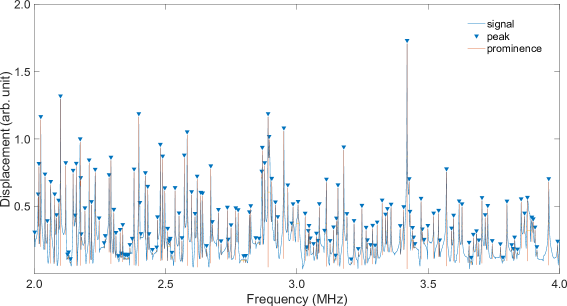
Figure S.9: $SiNx$ mode density

IV.2 Nature of added noise

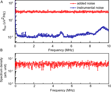
Figure S.10: Flat noise spectrum:(A) Experimental data for added white noise (red) and instrumental noise (blue). (B) White noise spectrum of numerical random function.

To test rigidity of time crystalline phases we feed in noise across the capacitive arrangement and record the spectrum with increasing r.m.s. amplitude of the noise ($V_{r.m.s.}$). Experimentally noise is added using a function generator. To understand the nature of noise, we look at Fourier transform of added noise. Blue curve in Fig. S.10A is instrumental noise floor without any added noise for a large range of frequency (0 to 10 MHz). Added noise gives a flat spectrum (red curve in Fig. S.10A) for the same range.

For numerical analysis, we choose a random function to add noise to the system. Amplitude of the function is Gaussian for uniform time step. Fourier transform of this function also gives a flat spectrum. So we will use this function for further numerical analysis.

IV.3 Additive and multiplicative term from capacitive arrangement

Our system is kept in a capacitive arrangement and force is applied through metallic contacts of sample and back gate.

For simplicity of calculation, we rewrite equation S.4a for $\alpha=0$, adding linear damping ($\gamma$) and a force term $F(x,t)$:

$$\ddot{x}+\gamma\dot{x}+\omega_{0}^{2}x+\frac{\beta}{m}x^{3}=F(x,t).$$ (S.25)

Now, we will calculate force $F(x,t)$ acting on the sample due to applied voltage $V(t)$ to capacitor.

From [50] we adopt the equation for stored elastic energy of the system,

$$U_{el}=\frac{8EA\chi_{0}x^{2}}{3L}+\frac{64EAx^{4}}{9L^{3}}.$$ (S.26)

Here, $E,A,\chi_{0}$ and $L$ represent young modulus, cross sectional area, built in strain and diameter of the suspended material respectively.

So, total force due to this term is

$$F_{el}=-\frac{16EA\chi_{0}}{3L}x-\frac{256EA}{9L^{3}}x^{3}.$$ (S.27)

For a parallel plate capacitor, we can write

$$C(x)=\frac{\epsilon_{0}A}{(d_{0}-x)},$$ (S.28)

where, $\epsilon_{0}$ and $d_{0}$ represent permittivity of air and mean distance between parallel plates respectively.

Stored electrostatic energy can be expressed as

$$U_{es}=\frac{1}{2}C(x)V(t)^{2}=\frac{\epsilon_{0}AV^{2}}{2(d_{0}-x)},$$ (S.29)

where, $V(t)$ is applied voltage across capacitor plates.

So, force due to this term is

$$F_{es}=-\frac{\epsilon_{0}AV^{2}}{2(d_{0}-x)^{2}}.$$ (S.30)

We expand $F_{es}$ around $x_{0}$ up to first order [51];

$$F_{es}=-\frac{\epsilon_{0}AV^{2}}{2(d_{0}-x_{0})^{2}}+\frac{\epsilon_{0}AV^{2}}{(d_{0}-x_{0})^{3}}x_{0}-\frac{\epsilon_{0}AV^{2}}{(d_{0}-x_{0})^{3}}x+O[x^{2}].$$ (S.31)

So total force acting on the sample perpendicular to the surface is

$$F=F_{el}-F_{es}=-\frac{256EA}{9L^{3}}x^{3}+\left(\frac{\epsilon_{0}AV^{2}}{(d_{0}-x_{0})^{3}}-\frac{16EA\chi_{0}}{3L}\right)x+\frac{\epsilon_{0}AV^{2}}{2(d_{0}-x_{0})^{2}}-\frac{\epsilon_{0}AV^{2}}{(d_{0}-x_{0})^{3}}x_{0}.$$ (S.32)

If voltage varies over time ($V(t)=V_{DC}+V_{AC}+V_{noise}$), we can rewrite equation S.25:

$$\ddot{x}+\gamma\dot{x}+\left(\omega_{0}^{2}+\frac{16EA\chi_{0}}{3L}-\frac{\epsilon_{0}AV(t)^{2}}{(d_{0}-x_{0})^{3}}\right)x+\left(\frac{\beta}{m}+\frac{256EA}{9L^{3}}\right)x^{3}=\frac{\epsilon_{0}AV(t)^{2}(d_{0}-3x_{0})}{2(d_{0}-x_{0})^{3}}.$$ (S.33)

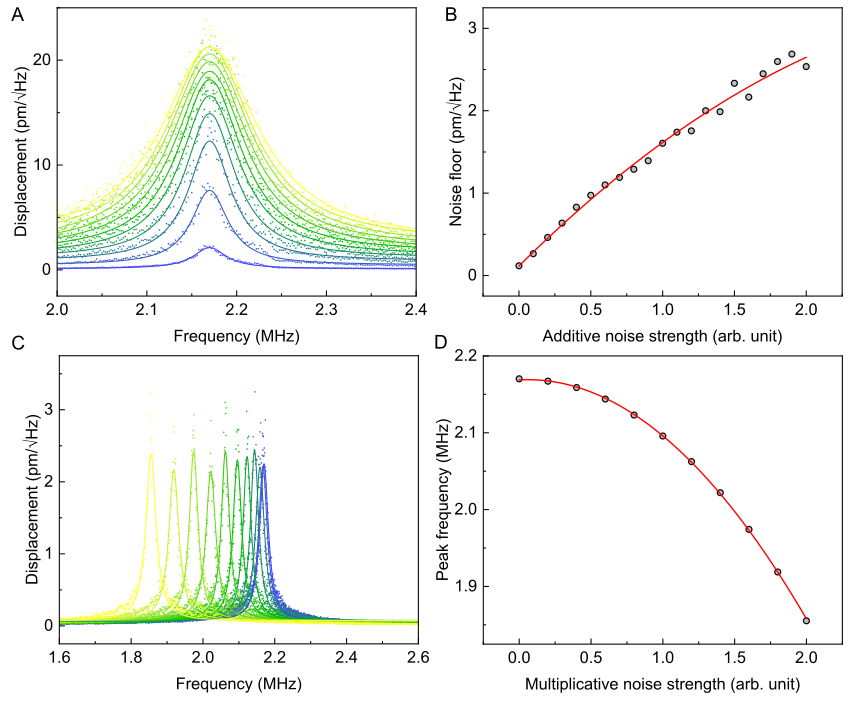
Figure S.11: Effect of noise: (A) Lorentzian fit on noise spectrum for increasing (from blue to yellow) values of added noise. (B) Change in noise floor with increasing additive noise strength. (C) Lorentzian fit on noise spectrum for increasing (from blue to yellow) values of multiplicative noise. (D) Frequency shift with increasing noise strength.

A time varying voltage across capacitive arrangement have two contribution to the equation of motion. One term modifies the frequency and other term acts as direct drive term.

IV.4 Noise axis calibration

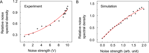
Figure S.12: Noise induced phase transition:(A) Experimental and (B) numerical relative noise spectral density vs input noise strength is plotted.

To compare experiment with numerical result, we need to calibrate noise strength axis. Experimentally we have observed that noise floor increases with increasing added noise strength. Similar things happens in numerical analysis if we consider additive noise term (see Fig. S.11A). We have seen earlier that capacitive force has a leading order term which acts as a force term. Lorentzian function is fitted on average spectrum of fifty iteration for different noise strength (see Fig. S.11A). Noise floor offset values are extracted as a fitting parameter and plotted against noise strength (see Fig. S.11B).

Next term of capacitive force is multiplicative. To understand higher order contribution we turn off additive term in numerical analysis and introduce multiplicative noise term. One must remember that in the case of multiplicative noise Milstein algorithm should be used instead of Euler–Maruyama algorithm. Here again lorentzian function is fitted on average spectrum of fifty iteration for different noise strength (see Fig. S.11C). Unlike experiment we observe non-linear frequency shift with increasing noise strength (see Fig. S.11D). Also note that here noise floor is remaining constant with increasing noise strength. So we can conclude that only leading order term of capacitive forcing is playing role in experiment when noise is added.

Now we can define a new parameter, relative noise spectral density, by taking ratio of extracted noise floor and maxima of thermal peak of the mode. As this is now unit-less quantity, this axis can be used as control parameter to observe phase transition in experiment and numerical analysis.

V Robustness to fluctuations

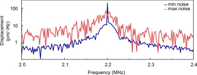
Figure S.13: Robustness of subharmonic phase: Numerical displacement spectral density shows subharmonic response (blue) gets destroyed slowly with increasing noise strength (red).

We focus on subharmonic phase to study robustness of the phase against added noise. In experiment the phase remains stable for certain threshold value of relative noise spectral density (Fig. 4A and B in main text). In numerical analysis, we observe similar nature of spectra (Fig. S.13) but do not observe sharp transition in the two-mode model (Fig. 4C in main text).

References

- [1] Anderson, P. W. More is different. Science 177, 393–396 (1972). URL https://www.science.org/doi/abs/10.1126/science.177.4047.393. eprint https://www.science.org/doi/pdf/10.1126/science.177.4047.393.
- [2] Shapere, A. & Wilczek, F. Classical time crystals. Phys. Rev. Lett. 109, 160402 (2012). URL https://link.aps.org/doi/10.1103/PhysRevLett.109.160402.
- [3] Else, D. V., Bauer, B. & Nayak, C. Floquet time crystals. Phys. Rev. Lett. 117, 090402 (2016). URL https://link.aps.org/doi/10.1103/PhysRevLett.117.090402.
- [4] Khemani, V., Lazarides, A., Moessner, R. & Sondhi, S. L. Phase structure of driven quantum systems. Phys. Rev. Lett. 116, 250401 (2016). URL https://link.aps.org/doi/10.1103/PhysRevLett.116.250401.
- [5] Yao, N. Y., Potter, A. C., Potirniche, I.-D. & Vishwanath, A. Discrete time crystals: Rigidity, criticality, and realizations. Phys. Rev. Lett. 118, 030401 (2017). URL https://link.aps.org/doi/10.1103/PhysRevLett.118.030401.
- [6] Goldstein, R. E. Coffee stains, cell receptors, and time crystals: Lessons from the old literature. Physics Today 71, 32–38 (2018). URL https://doi.org/10.1063/PT.3.4019. eprint https://doi.org/10.1063/PT.3.4019.
- [7] Mi, X. et al. Time-crystalline eigenstate order on a quantum processor. Nature 601, 531–536 (2022). URL https://doi.org/10.1038/s41586-021-04257-w.
- [8] Kyprianidis, A. et al. Observation of a prethermal discrete time crystal. Science 372, 1192–1196 (2021). URL https://www.science.org/doi/abs/10.1126/science.abg8102. eprint https://www.science.org/doi/pdf/10.1126/science.abg8102.
- [9] Bluvstein, D. et al. Controlling quantum many-body dynamics in driven rydberg atom arrays. Science 371, 1355–1359 (2021). URL https://www.science.org/doi/abs/10.1126/science.abg2530. eprint https://www.science.org/doi/pdf/10.1126/science.abg2530.
- [10] Maskara, N. et al. Discrete time-crystalline order enabled by quantum many-body scars: Entanglement steering via periodic driving. Phys. Rev. Lett. 127, 090602 (2021). URL https://link.aps.org/doi/10.1103/PhysRevLett.127.090602.
- [11] Else, D. V., Monroe, C., Nayak, C. & Yao, N. Y. Discrete time crystals. Annual Review of Condensed Matter Physics 11, 467–499 (2020). URL https://doi.org/10.1146/annurev-conmatphys-031119-050658. eprint https://doi.org/10.1146/annurev-conmatphys-031119-050658.
- [12] Khemani, V., Moessner, R. & Sondhi, S. L. A brief history of time crystals (2019). URL https://arxiv.org/abs/1910.10745.
- [13] Sacha, K. & Zakrzewski, J. Time crystals: a review. Reports on Progress in Physics 81, 016401 (2017). URL https://doi.org/10.1088/1361-6633/aa8b38.
- [14] Choi, S. et al. Observation of discrete time-crystalline order in a disordered dipolar many-body system. Nature 543, 221–225 (2017). URL https://doi.org/10.1038/nature21426.
- [15] Zhang, J. et al. Observation of a discrete time crystal. Nature 543, 217–220 (2017). URL https://doi.org/10.1038/nature21413.
- [16] Autti, S. et al. Nonlinear two-level dynamics of quantum time crystals. Nature Communications 13, 3090 (2022). URL https://doi.org/10.1038/s41467-022-30783-w.
- [17] Yao, N. Y., Nayak, C., Balents, L. & Zaletel, M. P. Classical discrete time crystals. Nature Physics 16, 438–447 (2020). URL https://doi.org/10.1038/s41567-019-0782-3.
- [18] Keßler, H. et al. Observation of a dissipative time crystal. Phys. Rev. Lett. 127, 043602 (2021). URL https://link.aps.org/doi/10.1103/PhysRevLett.127.043602.
- [19] Heugel, T. L., Oscity, M., Eichler, A., Zilberberg, O. & Chitra, R. Classical many-body time crystals. Phys. Rev. Lett. 123, 124301 (2019). URL https://link.aps.org/doi/10.1103/PhysRevLett.123.124301.
- [20] Ye, B., Machado, F. & Yao, N. Y. Floquet phases of matter via classical prethermalization. Phys. Rev. Lett. 127, 140603 (2021). URL https://link.aps.org/doi/10.1103/PhysRevLett.127.140603.
- [21] Pizzi, A., Nunnenkamp, A. & Knolle, J. Classical prethermal phases of matter. Phys. Rev. Lett. 127, 140602 (2021). URL https://link.aps.org/doi/10.1103/PhysRevLett.127.140602.
- [22] Gambetta, F. M., Carollo, F., Lazarides, A., Lesanovsky, I. & Garrahan, J. P. Classical stochastic discrete time crystals. Phys. Rev. E 100, 060105 (2019). URL https://link.aps.org/doi/10.1103/PhysRevE.100.060105.
- [23] Heugel, T. L., Eichler, A., Chitra, R. & Zilberberg, O. The role of fluctuations in quantum and classical time crystals (2022). URL https://arxiv.org/abs/2203.05577.
- [24] Bachtold, A., Moser, J. & Dykman, M. I. Mesoscopic physics of nanomechanical systems. Rev. Mod. Phys. 94, 045005 (2022). URL https://link.aps.org/doi/10.1103/RevModPhys.94.045005.
- [25] Faraday, M. Xvii. on a peculiar class of acoustical figures; and on certain forms assumed by groups of particles upon vibrating elastic surfaces. Philosophical Transactions of the Royal Society of London 121, 299–340 (1831). URL https://app.dimensions.ai/details/publication/pub.1026673574.
- [26] Karabalin, R. B., Cross, M. C. & Roukes, M. L. Nonlinear dynamics and chaos in two coupled nanomechanical resonators. Phys. Rev. B 79, 165309 (2009). URL https://link.aps.org/doi/10.1103/PhysRevB.79.165309.
- [27] Nayfeh, A. H. & Mook, D. T. Parametrically Excited Systems, chap. 5, 258–364 (John Wiley & Sons, Ltd, 1995). URL https://onlinelibrary.wiley.com/doi/abs/10.1002/9783527617586.ch5. eprint https://onlinelibrary.wiley.com/doi/pdf/10.1002/9783527617586.ch5.
- [28] Lifshitz, R. & Cross, M. C. Nonlinear Dynamics of Nanomechanical and Micromechanical Resonators, chap. 1, 1–52 (John Wiley & Sons, Ltd, 2008). URL https://onlinelibrary.wiley.com/doi/abs/10.1002/9783527626359.ch1. eprint https://onlinelibrary.wiley.com/doi/pdf/10.1002/9783527626359.ch1.
- [29] Heugel, T. L. Parametrons: From Sensing to Optimization Machines. Ph.D. thesis, ETH Zurich (2022). URL https://doi.org/10.3929/ethz-b-000543175.
- [30] Yao, N. Y. & Nayak, C. Time crystals in periodically driven systems. Physics Today 71, 40–47 (2018). URL https://doi.org/10.1063/PT.3.4020. eprint https://doi.org/10.1063/PT.3.4020.
- [31] Estarellas, M. P. et al. Simulating complex quantum networks with time crystals. Science Advances 6, eaay8892 (2020). URL https://www.science.org/doi/abs/10.1126/sciadv.aay8892. eprint https://www.science.org/doi/pdf/10.1126/sciadv.aay8892.
- [32] Nicolaou, Z. G. & Motter, A. E. Anharmonic classical time crystals: A coresonance pattern formation mechanism. Phys. Rev. Research 3, 023106 (2021). URL https://link.aps.org/doi/10.1103/PhysRevResearch.3.023106.
- [33] Bello, L., Calvanese Strinati, M., Dalla Torre, E. G. & Pe’er, A. Persistent coherent beating in coupled parametric oscillators. Phys. Rev. Lett. 123, 083901 (2019). URL https://link.aps.org/doi/10.1103/PhysRevLett.123.083901.
- [34] Kuramoto, Y. Self-entrainment of a population of coupled non-linear oscillators. In Araki, H. (ed.) International Symposium on Mathematical Problems in Theoretical Physics, 420–422 (Springer Berlin Heidelberg, Berlin, Heidelberg, 1975).
- [35] Acebrón, J. A., Bonilla, L. L., Pérez Vicente, C. J., Ritort, F. & Spigler, R. The kuramoto model: A simple paradigm for synchronization phenomena. Rev. Mod. Phys. 77, 137–185 (2005). URL https://link.aps.org/doi/10.1103/RevModPhys.77.137.
- [36] Leuch, A. et al. Parametric symmetry breaking in a nonlinear resonator. Phys. Rev. Lett. 117, 214101 (2016). URL https://link.aps.org/doi/10.1103/PhysRevLett.117.214101.
- [37] Singh, R., Nicholl, R. J. T., Bolotin, K. I. & Ghosh, S. Motion transduction with thermo-mechanically squeezed graphene resonator modes. Nano Letters 18, 6719–6724 (2018). URL https://doi.org/10.1021/acs.nanolett.8b02293.
- [38] Singh, R. et al. Giant tunable mechanical nonlinearity in graphene–silicon nitride hybrid resonator. Nano Letters 20, 4659–4666 (2020). URL https://doi.org/10.1021/acs.nanolett.0c01586. PMID: 32437616, eprint https://doi.org/10.1021/acs.nanolett.0c01586.
- [39] Seitner, M. J., Abdi, M., Ridolfo, A., Hartmann, M. J. & Weig, E. M. Parametric oscillation, frequency mixing, and injection locking of strongly coupled nanomechanical resonator modes. Phys. Rev. Lett. 118, 254301 (2017). URL https://link.aps.org/doi/10.1103/PhysRevLett.118.254301.
- [40] Romero, E. et al. Scalable nanomechanical logic gate (2022). URL https://arxiv.org/abs/2206.11661.
- [41] Faust, T., Rieger, J., Seitner, M. J., Kotthaus, J. P. & Weig, E. M. Coherent control of a classical nanomechanical two-level system. Nature Physics 9, 485–488 (2013). URL https://doi.org/10.1038/nphys2666.
- [42] Sillanpää, M. A., Park, J. I. & Simmonds, R. W. Coherent quantum state storage and transfer between two phase qubits via a resonant cavity. Nature 449, 438–442 (2007). URL https://doi.org/10.1038/nature06124.
- [43] Hajdušek, M., Solanki, P., Fazio, R. & Vinjanampathy, S. Seeding crystallization in time. Phys. Rev. Lett. 128, 080603 (2022). URL https://link.aps.org/doi/10.1103/PhysRevLett.128.080603.
- [44] Papariello, L., Zilberberg, O., Eichler, A. & Chitra, R. Ultrasensitive hysteretic force sensing with parametric nonlinear oscillators. Phys. Rev. E 94, 022201 (2016). URL https://link.aps.org/doi/10.1103/PhysRevE.94.022201.
- [45] Weber, P., Güttinger, J., Noury, A., Vergara-Cruz, J. & Bachtold, A. Force sensitivity of multilayer graphene optomechanical devices. Nature Communications 7, 12496 (2016). URL https://doi.org/10.1038/ncomms12496.
- [46] Dolleman, R. J., Davidovikj, D., Cartamil-Bueno, S. J., van der Zant, H. S. J. & Steeneken, P. G. Graphene squeeze-film pressure sensors. Nano Letters 16, 568–571 (2016). URL https://doi.org/10.1021/acs.nanolett.5b04251.
- [47] Manzaneque, T. et al. Resolution limits of resonant sensors with duffing non-linearity (2022). URL https://arxiv.org/abs/2205.11903.
- [48] Mahboob, I., Okamoto, H., Onomitsu, K. & Yamaguchi, H. Two-mode thermal-noise squeezing in an electromechanical resonator. Phys. Rev. Lett. 113, 167203 (2014). URL https://link.aps.org/doi/10.1103/PhysRevLett.113.167203.
- [49] Toral, R. & Colet, P. Numerical Simulation of Stochastic Differential Equations, chap. 7, 191–234 (John Wiley & Sons, Ltd, 2014). URL https://onlinelibrary.wiley.com/doi/abs/10.1002/9783527683147.ch7. eprint https://onlinelibrary.wiley.com/doi/pdf/10.1002/9783527683147.ch7.
- [50] Chen, C. Graphene NanoElectroMechanical Resonators and Oscillators. Ph.D. thesis, Columbia University (2013).
- [51] Lardies, J., Arbey, O. & Berthillier, M. Analysis of the pull-in voltage in capacitive mechanical sensors. In International Conference on Multidisciplinary Design Optimization and Applications (Paris, France, 2010). URL https://hal.archives-ouvertes.fr/hal-02300589.