Light-matter correlations in Quantum Floquet engineering

Abstract

Quantum Floquet engineering seeks to externally control systems by means of quantum fields. However, to faithfully capture the physics at arbitrary coupling, a gauge-invariant description of light-matter interaction is required, which makes the Hamiltonian highly nonlinear in the photonic operators. Here we provide a non-perturbative truncation scheme, which is valid for arbitrary coupling strength. With this framework, we investigate the role of light-matter correlations, which are absent in systems described by semiclassical Floquet engineering. We find that even in the high-frequency regime, their importance can be crucial, in particular for the topological properties of the system. As an example we show that in an SSH chain coupled to a cavity, light-matter correlations break chiral symmetry, strongly affecting the robustness of its edge states. In addition, we show how light-matter correlations are imprinted in the photonic spectral function, and discuss their relation with the topology of the photonic bands.

Introduction
Harnessing light-matter interactions has been a persistent goal in condensed matter physics and quantum technologies. A well-known example is the use of classical light to manipulate the properties of quantum systems, which we refer to as Semi-classical Floquet Engineering (SCFE) [1, 2, 3, 4, 5, 6, 7, 8, 9, 10, 11, 12, 13] or its variant to classical systems, known as Classical Floquet Engineering [14].
A recent scheme known as Quantum Floquet Engineering (QFE) [15, 16, 17, 18, 19] involves the use of quantum rather than classical light, in the context of what has been dubbed cavity quantum materials [20, 21, 22]. While both cases share some similarities [15], the back-action between the quantum system and the photon field, or the existence of light-matter correlations in the quantum case [23] can lead to physics beyond that of SCFE. Therefore, it is important to ask how these two pictures connect and to understand their differences.

Physically, SCFE can be seen as a limiting case of QFE where the light field is macroscopic [15], which implies that back-action is negligible and correlations are washed-out. However, it is conceptually very different from QFE because it is based on the presence of time-translation symmetry and the periodicity of the quasienergy bands [24]. In contrast, QFE is more challenging due to their many-body structure and to the highly nonlinear dependence on the photonic operators of the gauge-invariant Hamiltonians  [25, 26, 27, 28, 18, 15, 29, 16]. In fact, previous works in the field have proposed different methods to obtain simpler, effective Hamiltonians, such as mean-field ansatzs [19, 16] or high-frequency expansions for the matter part [18, 29, 15], with the preservation of gauge-invariance becoming a guiding line. Lastly, a key difference between the semiclassical and quantum regime is the issue of heating, inherent to SCFE  [30, 31, 32, 33, 34, 35, 36], which is expected to be mitigated in QFE [16, 20].

In the well-known field of SCFE, driven systems have revealed as fruitful platforms for creating and manipulating topological properties, being one of its most celebrated manifestations the presence of gapless boundary modes that are resilient to certain perturbations, in finite-size systems. This robustness encompasses many interesting physical phenomena, as well as promising applications for quantum technologies.
Then, by designing a suitable time-periodic driving, one can either tune the topology of a system [37, 3], induce non-trivial topological behaviour in an otherwise trivial set-up [38], or create unique phases with no static counterpart [39, 40, 41]. The classification of these driven topological phases can be systematically carried out in terms of symmetries and dimensionality, in the spirit of the well-known tenfold-way in the static case, with the associated topological invariants [42].

In QFE, the interplay between topology and quantized electromagnetic fields has not been explored to its fullest, and in particular, the effect of the interaction on the symmetries that support the topological phase remains an open question. This issue is not only crucial to QFE, but to any other set-up in which robust edge modes couple to quantum light, either for detection or for quantum information transfer protocols, since the breaking of a certain symmetry can jeopardize topological properties arising in the interacting system and their robustness.

In this context, the present work has a twofold aim. On the one hand, we present a general framework to obtain a non-perturbative, polynomial expansion of the full, gauge-invariant Hamiltonian based on the truncation of photon-exchange processes, which provides accurate results for arbitrary coupling strength. This method can successfully capture the physics of both, fermions and photons, in agreement with the predictions of gauge-invariant models. Importantly, it also keeps track of the role of light-matter correlations, which is not only essential to correctly predict the properties of the many-body system, but also to carry out a faithful comparison between SCFE and QFE.

On the other hand, we investigate QFE in the context of topological systems. As a proof of concept, we study the case of a Su-Schrieffer-Heeger (SSH) chain [43, 44] coupled to a cavity. We show how to produce edge states by tuning the light-matter coupling and the number of photons in the cavity and discuss the crucial role of light-matter correlations and how they affect topological protection and the fundamental symmetries of the system, even for a largely-detuned cavity [45]. Finally, we discuss how the spectroscopic analysis of the cavity can be used to detect our findings, and the possibility of using the cavity to control the electron transfer between edge states.

Results

Model
Consider a tight binding description of spinless fermions in a lattice, coupled to a single-mode cavity. The quantized electric field in the cavity can be expressed in terms of the vector potential $\vec{A}=A_{0}\left(d+d^{\dagger}\right)\hat{u}\left(r\right)$, where $\hat{u}$ is the unitary polarization vector Notice that we have assumed the dipole approximation, where the vector potential does not vary within the scale of the electronic system and its amplitude is independent of the spatial coordinate. In the Coulomb gauge and under a dipole approximation, the coupling between the two systems can be introduced via the Peierls substitution (see Supplementary Information, SI), yielding the Hamiltonian [46]:

$$H=\Omega d^{\dagger}d+\sum_{l,j=1}^{N}J_{l,j}e^{i\phi_{l,j}}c_{l}^{\dagger}c_{j}\ ,$$ (1)

with $\Omega$ is the cavity frequency, $N$ the number of sites in the array and $J_{l,j}$ the hopping. The creation/annihilation operators $c^{\dagger}_{j}$/$c_{j}$ are fermionic, while $d^{\dagger}$/$d$ are bosonic. In Eq. (1), the hopping gets dressed by the Peierls phase, $\phi_{l,j}=\eta_{l,j}\left(d^{\dagger}+d\right)$, with $\eta_{l,j}=eA_{0}r_{l,j}$ acting as the effective coupling strength ($e$ is the particle charge and $r_{l,j}$ is the distance between the $l^{\mathrm{th}}$ and $j^{\mathrm{th}}$ site). Notice that since $r_{l,j}=-r_{j,l}$, the coupling $\eta_{j,l}$ depends on both the distance between sites and the direction of the hopping.

Eq. (1) represents a gauge invariant description of the system for arbitrary coupling, but it is also highly nonlinear in the photonic operators, which makes its use difficult for practical calculations. Using the Baker-Haussdorf-Campbell formula, in combination with the Hubbard operators, $Y^{n,n^{\prime}}=|n\rangle\langle n^{\prime}|$, with $n,n^{\prime}\in\mathbb{Z}\geq 0$ and $|n\rangle$ the number of particle states, the Peierls phase can be rewritten as:

$$e^{i\eta_{l,j}(d^{\dagger}+d)}=\sum_{n=0}^{\infty}g_{n,n}^{l,j}Y^{n,n}+\sum_{n\neq m=0}^{\infty}g_{m,n}^{l,j}Y^{m,n},$$ (2)

where $g^{l,j}_{s,s}=e^{-\eta^{2}_{l,j}/2}L_{s}(\eta^{2}_{l,j})$, $L_{s}(\eta^{2}_{l,j})$ are the Laguerre polynomials, and the off-diagonal terms are given by the Hypergeometric functions ${}_{1}F_{1}(s,l,\eta^{2}_{l,j})$ (SI):

$$g_{s,m}^{l,j}=e^{-\eta_{l,j}^{2}/2}\frac{\left(i\eta_{l,j}\right)^{m-s}}{\left(m-s\right)!}\sqrt{\frac{m!}{s!}}\,_{1}F_{1}(s,m,\eta^{2}_{lm,j}).$$ (3)

Although the Krummer function is well-defined only for $m\geq s$, a numerical calculation of the exact matrix elements shows that they are symmetric $g^{j,i}_{s,m}=g^{j,i}_{m,s}$. After all these manipulations Eq. (1) becomes:

$$H= \sum_{n=0}^{\infty}(n\Omega+\sum_{\langle j,l\rangle=1}^{N}g_{n,n}^{l,j}J_{j,l}c_{j}^{\dagger}c_{l})Y^{n,n}$$

$$+\sum_{n\neq m=0}^{\infty}\sum_{\langle j,l\rangle=1}^{N}g^{l,j}_{m,n}J_{j,l}c_{j}^{\dagger}c_{l}Y^{m,n}\ ,$$ (4)

where the first line can be interpreted as a state-dependent frequency shift and the second as photon-assisted hopping. Note that Eq. (4) is a non-perturbative polynomial expansion in photon operators. For this reason, exact diagonalization is far more efficient with Eq. (4) than with Eq. (1), as numerically exact results require a SIaller number of photons $n_{\text{max}}$ to converge.

To make this Hamiltonian simpler, we propose to truncate the photon exchange to include only one-photon transitions, i.e., $m=n\pm 1$ in the second term. This is specially well-suited for the high-frequency regime $\Omega\gg J^{\prime},J$, where the hybridization between bands with a different number of photons is SIall, but also in the presence of resonances involving mostly one-photon exchange. The truncation of the total Hamiltonian not only improves the numerical efficiency of the calculations, but also enables analytical derivations that would be intractable otherwise, while offering a valuable physical insight on the physics of the interacting system, as we will see below.

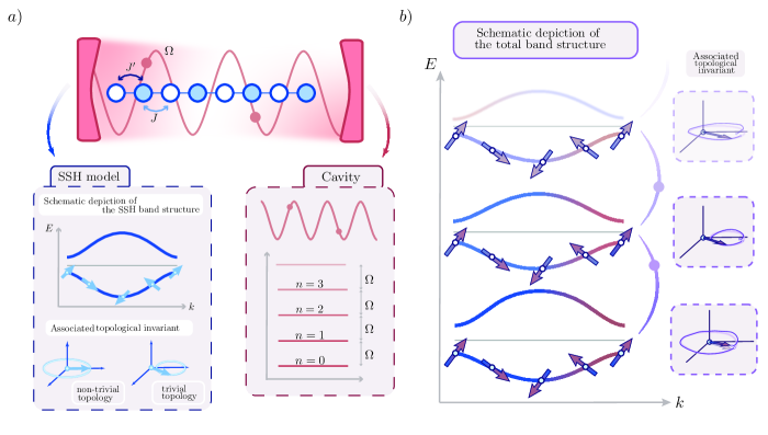
Figure 1: $a)$ Schematic representation of the system: an SSH chain (in blue) interacting with a photonic field in a cavity (in red). On the one hand, the SSH consists on alternating hopping amplitudes, $J^{\prime}$ and $J$, whose ratio define two distinct topological phases. The latter can be identified by the value of the topological invariant, which can be represented as a winding number in parameter space. On the other hand, the photonic field is defined by its frequency $\Omega$, and its energy levels determined by the number of photons $n$ in the cavity. $b)$ The resulting band structure of the total system corresponds to sucessive photonic subspaces where the electronic energy levels are renormalized differently. The presence of photon-exchange processes induces a certain effective coupling between (purple lines), which has a direct impact on the topological invariant.

SSH Hamiltonian
While this approach is general for arbitrary lattice systems, here we are interested in topological ones. Then, we particularize to a bipartite lattice or SSH chain [43, 44], with different intra- and the inter-dimer hopping amplitudes, $J_{2j-1,2j}=J_{2j,2j-1}\equiv J^{\prime}$ and $J_{2j,2j+1}=J_{2j+1,2j}\equiv J$, respectively (SI). Here, $j=1,2,...,2N$ is a site index, and $2N$ is the total number of sites, being $N$ the number of unit cells. This leads to the definition of two distinct sublattices, $A$ and $B$, and their corresponding creation/annihilation operators ($c^{(\dagger)}_{2j-1}\rightarrow a^{(\dagger)}_{p}$ and $c^{(\dagger)}_{2j}\rightarrow b^{(\dagger)}_{p}$, where $p=1,...,N$ is a cell index). With this, the SSH Hamiltonian gives

$$H_{\mathrm{SSH}}=\sum_{l=1}\left(J^{\prime}a^{\dagger}_{p}b_{p}+Ja^{\dagger}_{p+1}b_{p}+\text{h.c.}\right).$$ (5)

The SSH model is a canonical example for topological insulators in one dimension [47, 48], showcasing two distinct topological phases as a function of the ratio $J^{\prime}/J$. For the topological phase, $J^{\prime}/J<1$, two edge states appear within the gap, that are topologically protected by chiral symmetry [49]. The hopping dimerization implies a different intra/inter-dimer distance, $r^{\prime}$ and $r$ (the unit cell length is set to $r+r^{\prime}=1$), which gives a dimerized coupling that depends on either $r$ or $r^{\prime}$: $\eta^{(\prime)}=eA_{0}r^{(\prime)}$. This has well-known consequences for the topology of the chain in SCFE [3].
Chiral symmetry is an important symmetry in 1D topological systems, as it can provide for topological protection. This is the case of the SSH model, displaying time-reversal, particle-hole and chiral symmetries [47, 48]. In particular, the later can be represented by an unitary operator $\Gamma$ that anti-commutes with the fermionic Hamiltonian. For the case of the SSH chain, $\Gamma H_{\mathrm{SSH}}\Gamma=-H_{\mathrm{SSH}}$, the chiral operator can be expressed as $\Gamma=\sigma_{z}$. This implies that on-site potential must be uniform and that hopping terms must connect sites between different sublattices only [49].

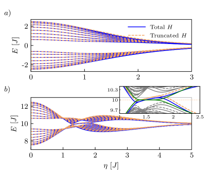
Figure 2: Energy spectrum obtained from exact, numerical diagonalization (Eq. 4) of the $a)$ $n=0$, and $b)$ $n=1$ subspaces of the SSH Hamiltonian in a cavity, for the total (blue) and truncated (dashed, orange) Hamiltonians. Inset: zoom into the edge states energy, also considering the mean-field spectrum (green). Parameters: $J^{\prime}=1.5$, $J=1$, $r^{\prime}=0.4$, $\Omega=10$, $n_{\mathrm{max}}=70$ (maximum number of photonic subspaces included for convergence), $N=16$.

High-frequency (HF) regime in QFE
Fig. 2 shows the spectrum of the system in the HF regime $\Omega\gg J^{\prime},J$, as a function of the coupling $\eta$. It shows excellent agreement between the exact diagonalization of Eq. (4) and its truncated version to one-photon processes, for all values of the coupling (see SI for the resonant case $\Omega\sim J^{\prime},J$, which can also be captured with the truncated Hamiltonian). The spectrum also shows the cavity-induced localization (band collapse) at large coupling, produced by the exponential suppression of the hopping in Eq. (3). Quantitative SIall differences between them are due to multi-photon exchange processes (SI). Importantly, the hopping of the unperturbed SSH chain in Fig. 2 is such that the system is topologically trivial for $\eta=0$. Then, while the subspace with $n=0$ photons in the $a)$ panel always lacks edge states, the $b)$ panel shows that in the subspace with $n=1$ photons, increasing $\eta$ gives rise to the appearance of edge states.

This effect resembles the topological phase transition of the SSH chain in the HF regime of SCFE [3], where robust edge states appear for certain field amplitudes. In fact, the effect of both classical and quantum light on electronic systems can be easily connected using the formalism of Eq. 1. As shown in Ref. [15], the crossover from QFE to SCFE can be investigated by taking the limit of large photon numbers $n\rightarrow\infty$. Then, the previously defined vector potential $\vec{A}=A_{0}(d^{\dagger}+d)\hat{u}_{r}$ turns into the coherent field $\vec{A}_{\mathrm{c}}=A_{0,\mathrm{c}}\cos(\Omega t)\hat{u}_{r}$ with amplitude $A_{0,c}$ and frequency $\Omega$, while the Peierls phase in Eq. 1 becomes time-dependent $\phi_{l,j}(t)=A_{0,c}\cos(\Omega t)r_{l,j}$. However, despite their similarities, important differences between the two situations are present, and we will explore them in the fore-coming sections.

Comparison between SCFE and QFE
The first important difference between SCFE and QFE is that the spectrum in SCFE, due to time periodicity, consists on infinite copies of identical Floquet bands. In contrast, in the present case the spectrum is bounded from below and each photonic subspace renormalizes differently, as a function of $\eta$. This distinction is resolved in the limit of $n\to\infty$, where the differences between bands in QFE vanish and the Bessel functions renormalization is recovered [15]. This shows that QFE provides additional external control, as the number of photons in the cavity can now be used to manipulate the system as well. Importantly, as the spectrum of QFE is bounded from below, it has a well-defined ground state, as opposed to SCFE.

A second difference is related to the calculation of an effective matter Hamiltonian in the HF regime. Typically, in SCFE one can find a stroboscopic time-evolution operator described by an effective Hamiltonian with renormalized parameters, which can be derived by means of a Magnus expansion in inverse powers of the drive frequency [50]. In QFE, such effective Hamiltonians for either the cavity photons or the electronic system can be obtained by performing a mean-field (MF) approximation, as suggested in previous works [16, 19]. In the MF Hamiltonians, back-action due to the interaction is contained in the renormalization of the parameters of each subsystem, while the effect of light-matter correlations is neglected. In this sense, the MF result for QFE can be equated to SCFE, since both of them lack quantum correlations (the only difference between MF and SCFE is the back-action from the fermions onto the cavity, due to the MF self-consistency equations). However, we will see below why fluctuations are important and should be included in the case of QFE, especially when dealing with topological systems.

The reason is rooted in the third essential difference between SCFE and QFE, which concerns the fate of chiral symmetry in each case.
For SCFE in the HF regime, one finds that the effective Hamiltonian preserves chiral symmetry, which is why the edge states are at zero energy and topologically protected [3]. Being the effective Hamiltonian time-independent, its symmetries can be analyzed as in any static system.
For the MF approach to QFE, the same conclusion is obtained [16]: the MF Hamiltonian for the electronic system preserves chiral symmetry, since it retains the off-diagonal form of the unperturbed SSH Hamiltonian (SI),

$$(H_{n})_{\mathrm{SSH}}^{\mathrm{MF}}=\sum_{p=1}\left(\tilde{J}^{\prime}_{n}a^{\dagger}_{p}b_{p}+\tilde{J}_{n}a^{\dagger}_{p+1}b_{p}+\text{h.c.}\right),$$ (6)

where $\tilde{J}^{(\prime)}_{n}=J^{(\prime)}L_{n}\left(\eta^{(\prime)2}\right)$ are the renormalized hopping amplitudes. Note that there is a dependence on the photonic subspace $n$ considered. This is because an effective MF Hamiltonian can be derived for each Fock subspace, accounting for the different dressing of the electronic band structure depending on the cavity state preparation.
The MF Hamiltonian preserves the off-diagonal structure, which means that the chiral-symmetry operator can be defined again as $\Gamma=\sigma_{z}$, in the same basis as for $H_{\mathrm{SSH}}$ in Eq. 5. In fact, we show the MF result for the edge states in the first photonic band in Fig. 2, inset of panel $b)$ (green): the edge states remain pinned to the middle of the gap, despite the increase in the coupling strength, confirming the presence of chiral symmetry and topological protection.

However, QFE has an additional ingredient that is neglected in a MF analysis and absent by definition in SCFE: light-matter correlations. Although they are expected to be SIall for $\Omega\gg J$, $J^{\prime}$, for topological systems one must be careful, because the topological protection of edge states might be linked to symmetries that are broken by these corrections. This is the case of the SSH chain, as we show as well in the inset of Fig. 2: there, one can see that the pair of degenerate edge states obtained from exact numerical diagonalization of the Hamiltonian, moves from the center of the gap, hybridizing with the bulk bands and indicating the breaking of chiral symmetry. Inversion symmetry remains intact, which is why the edge states remain degenerate. This effect is analogous to that of long-range hopping in an SSH chain [49]. The comparison with the MF result confirms that this is a consequence of light-matter correlations.

From the form of the Peierls phase in Eq. 1, one could think that gauge-invariant coupling to light in lattice Hamiltonians conserves chiral symmetry, because the block-structure of the matter Hamiltonian is not changed by the Peierls phase or the renormalized hopping. The breaking of chiral symmetry in the Coulomb gauge, and the physical process behind, must be analyzed considering both photons and fermions, i.e., taking the interacting system as a whole. Therefore, it is not enough to study the electronic part alone. A complete characterization of the topological phase, as well as a quantization of the impact of light-matter correlations on topological properties, can be carried out by means of the topological invariant for the full system. For this, let us point out that the truncated Hamiltonian captures the breaking of chiral symmetry, as shown by the numerical results, which further confirms that it can be used to study the system and its topological properties. Additionally, the speed-up in the numerical treatment of Eq. (4) compared to the exact diagonalization of the Peierls Hamiltonian in Eq. (1) motivates the use of the former in the following sections (we have also checked its accuracy by comparing with the total Hamiltonian).

Topological invariant
In a non-interacting and isolated SSH chain, the topological phase is characterized by a topological invariant $\mathcal{W}$, which is a quantized Zak phase that a particle picks up when it is carried across the first Brillouin zone [51]. It takes the discrete values $\mathcal{W}=0$ in the trivial phase and $\mathcal{W}=1$ in the topological one, and has a one-to-one correspondence with the number of pairs of edge states within the gap [52].

This topological invariant can be calculated as the winding number arising from the trajectory of the Bloch vector (see Fig. 1$a)$ for an schematic representation), but it has been shown that Green’s functions (GFs) provide an alternative approach, with the possibility to incorporate many-body effects [53, 54, 55, 56, 57]. Importantly, its value converges to the standard winding number in the non-interacting limit. In particular, the winding number for the SSH chain in terms of Green’s functions can be written as:

$$\mathcal{W}=\frac{1}{4\pi i}\int_{-\pi}^{\pi}dk\hskip 2.0pt\Gamma[\hat{G}(k,0)]^{-1}\partial_{k}\hat{G}(k,0).$$ (7)

where we have defined the matrix $\hat{G}(k,\omega)$ as the Fourier transform of the retarded Green function with matrix elements $G_{\alpha,\beta}(k,t)=-i\theta(t)\langle\{\alpha_{k}(t),\beta_{k}^{\dagger}\}\rangle$ and $\alpha,\beta=A,\hskip 2.0ptB$ the sub-lattice index. Note that the fermionic creation/annihilation operators are now written in $k$ space. Notice that this definition of $\mathcal{W}$ requires that the system displays chiral symmetry $\Gamma$.

Importantly, we can extended our previous discussion of the system in terms of MF plus fluctuations, to the calculation with Green’s functions, to determine the effect of light-matter correlations in the topological invariant. Additionally, for the case of the truncated Hamiltonian, it is possible to find analytical expressions and explicitly demonstrate the breaking of chiral symmetry due light-matter correlations.

In order to do this, first we must slightly generalize the expression for the Green’s function, to include the presence of photons from the cavity. We define the fermionic Green’s function, projected onto the $n$-th Fock band, as:

$$G^{n,n}_{\alpha,\beta}(k,t)=-i\theta(t)\langle\{\alpha_{k}(t)Y^{n,n},\beta_{k}^{\dagger}\}\rangle$$ (8)

Notice that it is now a many-body Green’s function with fermionic and photonic components. Let us first, show how the non-interacting limit is recovered from Eq. 8. For $\eta^{\prime}=0$, the distint Fock subspaces are decoupled, and the energy spectrum consists on infinitely many copies of the electronic band structure separated by an energy splitting of $\Omega$. Each eigenstate has a well-defined photon number $m$, and can be factorized between a fermionic part $|\psi(k)\rangle$ and a photonic one $|m\rangle$, yielding $|\Psi(k)\rangle=|\psi(k)\rangle\otimes|m\rangle$. Therefore, in this limit, if one wishes to calculate $G^{m,m}(k,\omega)$, only the eigenstates such that $\langle m|\Psi_{i}\rangle=1$ will give a non-zero contribution as if we were considering an isolated SSH chain.

A similar conclusion can be obtained for the MF Hamiltoninan, which depends on the cavity preparation through a photon index, but does not include any photon-exchange terms. The calculation of the corresponding GF shows that it takes a chiral form that commutes with $\Gamma=\sigma_{z}$ when evaluated at $\omega=0$, as expected:

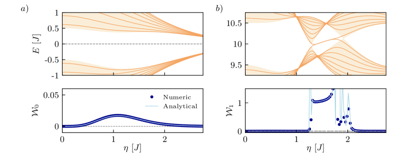
Figure 3: Loss of chiral symmetry due to electron-photon correlations, as reflected in the energy spectrum and the topological invariant of each photonic band: $a)$ $n=0$, and $b)$ $n=1$. The shaded regions in the top plots indicate the width of the corresponding energy band in the thermodynamic limit. In the bottom plots, the topological invariant is shown for both the numerical and the anaylitical solution of $G^{n,n}(k,\omega)$. $J^{\prime}=1.5$, $J=1$, $r^{\prime}=0.4$, $n_{\mathrm{max}}=80$, $N=16$.

$$\hat{G}_{\mathrm{MF}}^{n,n}(k,\omega)=\frac{1}{2\pi}\frac{1}{\omega^{2}-\varepsilon^{2}_{n}(k)}\left(\begin{array}[]{cc}\omega&h_{n}(k)\\ h^{*}_{n}(k)&\omega\end{array}\right),$$ (9)

where $\varepsilon^{2}_{n}=h^{*}_{n}(k)h_{n}(k)$ corresponds to the photo-dressed electronic band structure, with $h_{n}(k)=\tilde{J}^{\prime}_{n}+\tilde{J}_{n}e^{ik}$. For this reason, the calculation of the winding number for each photonic band, which can also be generalized to

$$\mathcal{W}_{n}=\frac{1}{4\pi i}\int_{-\pi}^{\pi}dk\hskip 2.0pt\Gamma[G^{n,n}(k,0)]^{-1}\partial_{k}G^{n,n}(k,0),$$ (10)

perfectly predicts the existence of topological edge states from the MF Hamiltonian. Its value not only depends on the coupling $\eta$, due to the dressing of the electronic band structure, but also on the band index $n$, as predicted from the MF Hamiltonian.

Including quantum correlations encoded in photon exchange processes complicates the calculation, but for the truncated Hamiltonian one can show analytically that the corresponding GF takes a non-chiral form, with no operator satisfying $\Gamma\hat{G}^{n,n}(k,0)\Gamma=-\hat{G}(k,0)$ (SI). From this result we can conclude that light-matter correlations induced by the exchange of spectral weight between different photonic bands are responsible for the breaking of chiral symmetry in the interacting systems. When the electronic part has topological properties, this is of a crucial importance: it means that topological protection, if provided by chiral symmetry, will be lost due to the nature of the photon field. In consequence, the winding number losses its quantization.

This is shown in Fig. 3, where we plot $\mathcal{W}_{0}$ and $\mathcal{W}_{1}$ (lower panels) together with the detail of the asymmetry induced by the coupling with the cavity photons in the energy spectrum (upper panels). First, let us remark that the agreement between the numerical and the analytical solution is excellent. Importantly, both $\mathcal{W}_{0}$ and $\mathcal{W}_{1}$ capture the breaking of chiral symmetry through the loss of quantization: note how the asymmetry in the spectrum is proportional to the deviations from integer values in the topological invariant, in both cases. This is specially evident in panel $a)$, where the maximum asymmetry corresponds to the maximum value of $\mathcal{W}_{0}$. Similarly, in the topological region of panel $b)$, $\mathcal{W}_{1}$ takes the closest values to $1$ when the deviation of the energy are minimal, i.e., chiral symmetry is weakly broken. Besides, the values of $\mathcal{W}_{0,1}\sim 0$ or $1$ are linked to the presence of edge states, and reflect the phase transition in the finite system.

To conclude, the breaking of chiral symmetry is also evident if one transforms Eq. 1 to the dipole gauge (SI), which yields

$$H_{\mathrm{DG}} = \Omega d^{\dagger}d+H_{el}+ieA_{0}\Omega(d-d^{\dagger})\sum_{i}r_{i}c^{\dagger}_{i}c_{i}$$

$$+eA_{0}\Omega\left(\sum_{i}r_{i}c^{\dagger}_{i}c_{i}\right)^{2}$$

While gauge invariance ensures that the physical results are independent of the choice of gauge, the form of the light-matter coupling is gauge dependent. In the previous expression, the interaction with photons in the cavity shifts the energy of each site of the chain (last term in first line) through the action of the displacement field $\Pi\propto i(d-d^{\dagger})$. Also, an additional photon-assisted density interaction term (second line) that affects only the electronic subsystem must be included to keep gauge invariance for arbitrary coupling strength [58]. Therefore, the presence of a photon-induced on-site potential in the fermionic system, either through the creation and destruction of photons (last term in first line) or through a self-interaction term (second line), indicates that chiral symmetry is broken in the hybrid system. In fact, there is not an operator $\Gamma$ satisfying $\Gamma H_{\mathrm{DG}}\Gamma=-H_{\mathrm{DG}}$.

Detection of light-matter correlations
A well-known experimental observable in cavity QED is the frequency shift produced by the interaction with the quantum system, which can be used to perform quantum non-demolition measurements [59, 60, 61, 62]. Its value can be extracted from the photon spectral function $A(\omega)=-\frac{1}{\pi}\text{Im}\int dte^{-i\omega t}D(t)$, which can be experimentally measured by detection of the photons in the cavity, being $D(t)=-i\theta(t)\langle[d(t),d^{\dagger}]\rangle$ the photonic Green’s function.

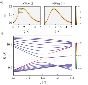
Figure 4: $a)$ Exact (left, obtained with the truncated Hamiltonian) and mean field (right) value of $A(\omega)$ as a function of $\eta$ for a cavity with $n=0$. The chain is in its ground state for a trivial phase configuration. $b)$ Truncated spectrum of the $n=1$ subspace vs $\eta$. The color code indicates the effective cavity-mediated interaction strength $\mathcal{P}_{i}$ between the ground state $|\Psi_{\mathrm{0}}\rangle$ and the $i^{\mathrm{th}}$ eigenstate in the $n=1$ subspace. Parameters: $J^{\prime}=1.5$, $J=1$, $r^{\prime}=0.4$, $\Omega=10$, $n_{\mathrm{max}}=70$, $N=16$.

Now we describe how the spectroscopy of photons can be used to detect light-matter correlations and how they encode information about the edge states in the system.
In Fig. 4 $a)$ we consider the cavity in its vacuum state and, to isolate the role of light-matter correlations, we compare the exact spectral function $D_{\mathrm{e}}$ (left, obtained from the truncated Hamiltonian) with the MF case $D_{\mathrm{MF}}$ (right). It shows that, for the chain in its ground state, MF correctly captures the frequency shift (details of the calculation in the SI):

$$\delta\Omega=\sum_{j,l}J_{j,l}e^{-\eta^{2}_{l,j}/2}\langle c_{j}^{\dagger}c_{l}\rangle,$$ (12)

but fails to capture the fine spectral details near $\eta\sim 1.3$, originated by light-matter correlations (framed region in the left plot). The mechanism enhancing light-matter correlations in this region is illustrated in Fig. 4 $b)$, which shows the truncated spectrum in the $n=1$ subspace, as the light-matter coupling increases. The color code indicates the effective cavity-mediated interaction between the ground state of the system, $|\Psi_{0}\rangle$, and the $i^{\mathrm{th}}$ state in the $n=1$ subspace, $|\Psi^{(1)}_{i}\rangle$ $(i=1,...,2N)$, calculated as $\mathcal{P}_{i}=|\langle\Psi_{0}|d|\Psi^{(1)}_{i}\rangle|^{2}$.

Initially, the interaction with the $n=1$ subspace is mainly with the state on top of the valence band. However, as $\eta$ increases, this state becomes an edge state near $\eta\sim 1.3$ and since the edge states are exponentially decoupled from the bulk [63], the interaction jumps to the state at the bottom of the conduction band, producing the correction to the MF result (see Fig.4 )

Importantly, if instead the chain is in the topological phase for $\eta=0$, the relation between the topological phase transition and the enhancement of light-matter correlations in $A(\omega)$ still holds. Thus, it can be verified regardless of the chain being prepared in either its trivial or topological phase. Let us now consider the case of the chain being initially prepared in one of each edge states, in the topological phase. The result for $D(\omega)$ is shown in Fig. 5, considering the subspace of $n=0$ photons (note that for the topological phase, the edge states in this photonic subspace do not disappear as a function of $\eta$, as in Fig. 2).

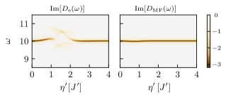
Figure 5: $A(\omega)$ vs $\eta^{\prime}$ for an empty cavity. The left plot shows the exact spectral function, while the right plot shows the MF solution. The chain is prepared in an edge state. Parameters: $r^{\prime}=0.4$, $\Omega=10$, $n_{\mathrm{max}}=70$, $N=16$, $J^{\prime}=1$, $J=1.5$.

In this case, as the edge states are exponentially decoupled from the bulk, the cavity frequency does not shift [63]. However, when the edge states in the $n=1$ merge with the bulk, correlations strongly affect the MF value of $A(\omega)$, until the $n=1$ band becomes topological again. This means that we can use the cavity, not only to externally tune the presence of edge states but also to detect the presence of edge states in subspaces with a different number of photons using spectroscopy.

State transfer dynamics
As we discussed above, in the absence of chiral symmetry, the edge states in the SSH chain loose their topological protection, but this does not mean that they cannot be used for practical applications. It has been proposed that, as they are exponentially localized states, their SIall overlap between the two ends of the chain can be used in quantum state transfer [64, 65, 66, 67]. Now we show that in QFE, the cavity can be used to control charge dynamics by creating edge states in a trivial chain if $n>0$. This allows to implement state transfer protocols in systems that originally lack edge states, and fine-tune the transfer time between the two ends of the chain.

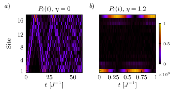
Figure 6: $a)$ Fermionic occupation probability $P_{i}(t)$ of each site of the chain $i=1,...,2N$ vs time, for a particle initially occupying the first site, $n=2$, and $\eta$=0. $b)$ $P_{i}(t)$ as a function of time, $\eta$=1.2 and $n=2$. Parameters: $J^{\prime}=1.5$, $J=1$, $r^{\prime}=0.4$, $N=16$, $\Omega=10$, $n_{\mathrm{max}}=50$.

This is shown in Fig. 6 $a)$, where a particle initially at site $1$ of an SSH chain in the trivial topological phase, freely evolves populating all sites of the chain. In contrast, the right panel shows that if the chain is coupled to a cavity with $n=2$ photons, there are coherent oscillations between the two ends, confirming the presence of cavity-induced edge states. (Note the change in the time scale between panels $a)$ and $b)$). This dynamics indicates that, although chiral symmetry is broken, the transfer between the two ends of the chain still is efficient. Importantly, the fine-tuning of the coupling strength and the number of photons provides additional means to control state transfer in this system (SI).

Discussion
We have shown that QFE is more complex than its classical counterpart, even in the case of large cavity frequency, where one expects that the cavity photons can be easily traced-out and light-matter correlations neglected, without relevant consequences.

Our work deals with a quite general question: what is the role of light-matter correlations in Quantum Floquet Engineering, and how does it allow us to go beyond classical Floquet engineering? This is in fact a relevant question, since light-matter correlations are, by definition, absent in the classical case, and can therefore set apart both cases. While some connections between the SCFE and QFE have been previously explored [16, 15], the particular role of light-matter correlations has been so far neglected in this context. For this, we have developed a non-perturbative truncation method to reduce the highly non-linear gauge-invariant Hamiltonian, to a simpler one that remains valid for arbitrary coupling and correctly detects changes in the symmetries that are relevant for the topology.

While this truncation scheme is general and valid for arbitrary lattice systems, we have considered a SSH chain coupled to the cavity to investigate the interplay between light-matter interaction and topological properties [68, 69, 45, 16]. We have shown that the interaction with the cavity can drive a topological phase transition, which can be controlled via the coupling strength and the number of photons in the cavity. The later is a tuning parameter absent in SCFE.

Importantly, using the SSH model as a benchmark, we demonstrate that light-matter interactions, quantum correlations and symmetries showcase an interesting interplay in these hybrid systems, even in the HF regime (this is in contrast with the HF regime of SCFE [3], where the coupling to light conserves the symmetries of the SSH chain). In general, chiral symmetry in 1D topological insulators plays a crucial role, as in many systems it protects the topological phase and the edge states.

The crucial point in our analysis is that the photon-assisted hopping introduces quantum light-matter correlations that are not captured by a mean-field approach, and break chiral symmetry. This is reflected in the band asymmetry and the shift in the edge states energy (Fig. 1) that the mean-field result does not capture. Therefore, it is not the hopping renormalization that shows the symmetry-breaking mechanism, but rather the presence of quantum many-body effects. The identification of a symmetry-breaking mechanism due to quantum fluctuations in the system could set an important milestone in the field of cavity- quantum materials, and can have important implications for the detection and generation of topological phases in hybrid light-matter platforms. In fact, this is not only important for topological insulators, but also for topological superconducting systems. In this later case, the coupling with light has also been explored as an alternative route to elucidate the existence of Majorana states which could be jeopardized by the presence of symmetry-breaking processes [70, 71, 72].

In addition, we have found that light-matter correlations can be experimentally detected in the photon spectral function, and that they contain information about the cavity-induced topological phase transitions in the system. This is a consequence of the different response of bulk and edge states to the presence of cavity photons [63]. Finally, we have shown that the cavity also provides us with a way to control the state transfer between edges of the chain. It can be used to create or destroy the edge states, as well as to tune the transfer time between the two sides.
As an outlook, we can envision future research lines derived from our findings. For example, the use of the formalism to study systems with electron-electron interaction, or the role of dissipation.

Acknowledgments
G.P. and B.P.G. acknowledge the Spanish Ministry of Economy and Competitiveness for financial support through the grant: PID2020-117787GBI00. A.G.L acknowledges support from the European Union’s Horizon 2020 research and innovation program under Grant Agreement No. 899354 (SuperQuLAN). All the authors also acknowledge support from CSIC Interdisciplinary Thematic Platform on Quantum Technologies (PTI-QTEP+).

Author Contributions
B. P. G. did the analytical and numerical analysis under the supervision of A. G. L. and G. P. All authors discussed and analyzed the results, and contributed to the writting of the final paper.

Additional Information
Competing financial interests: The authors declare no competing financial interests.

Appendix A LIGHT-MATTER COUPLING IN THE COULOMB AND DIPOLE GAUGE

The starting point is the tight-binding Hamiltonian $H_{\mathrm{el}}=\sum_{ij}^{N}J_{i,j}c_{i}^{\dagger}c_{j}$ that is coupled to a single-mode photonic field $H_{\mathrm{phot}}=\Omega d^{\dagger}d$. In general, the minimal-coupling Hamiltonian describing the light-matter interaction in the Coulomb gauge can be implemented through an unitary transformation $U$ acting on the fermionic degrees of freedom only [25, 46, 28], with

$$U=\mathrm{exp}\left\{i(d^{\dagger}+d)\sum_{ij}\chi_{ij}c^{\dagger}_{i}c_{j}\right\}$$ (13)

where $\chi_{ij}=\langle i|\chi|j\rangle=\int d\vec{r}\phi^{*}_{i}(\vec{r})\chi(\vec{r})\phi_{j}(\vec{r})$, being $\phi_{i}(\vec{r})$ the single-particle wavefunctions localized around each lattice site $i$, and $\chi(\vec{r})$ chosen such that $\nabla\chi(\vec{r})=eA_{0}(\vec{r})$, or equivalently,

$$\chi(\vec{r})=e\int_{\vec{r}_{0}}^{\vec{r}}A_{0}(\vec{r}^{\prime})\cdot d\vec{r}^{\prime}$$ (14)

In general, the vector potential in a 1D system can be written as $\vec{A}(r)=A_{0}(r)(d^{\dagger}+d)\hat{u}(r)$, where $A_{0}=1/\sqrt{2\varepsilon_{0}\Omega\nu}$ $(\hbar=1)$, with $\varepsilon_{0}$ being the vacuum permittivity and $\nu$ the cavity volume. Under the dipole approximation used in the main text $A_{0}(r)\approx A_{0}$, and assuming that the vector potential is orientated along the axis of the electronic chain (without loss of generality, we will assume this is the $x$ axis), this expression can be further simplified to yield $\chi(r)=eA_{0}r$, where we have dropped the vectorial notation for the position coordinate (we have also taken $r_{0}=0$). Therefore, we can also write $\chi_{ij}\approx\delta_{ij}\chi_{ii}=eA_{0}r_{i}\delta_{ij}$, and the final form of the transformation $U$ is

$$U=\mathrm{exp}\left\{ieA_{0}(d^{\dagger}+d)\sum_{i}r_{i}c^{\dagger}_{i}c_{i}\right\}$$ (15)

Using the Baker-Campbell-Hausdorff formula, the transformed fermionic operators will then give

$$U^{\dagger}c_{i}U=c_{i}e^{ieA_{0}r_{i}(d^{\dagger}+d)},\hskip 3.0ptU^{\dagger}c_{i}^{\dagger}U=c_{i}^{\dagger}e^{-ieA_{0}r_{i}(d^{\dagger}+d)}$$ (16)

The Peierls Hamiltonian $H$ shown in Eq. $(1)$ in the main text can be obtained by operating $H_{\mathrm{PS}}=H_{\Omega}+U^{\dagger}H_{\mathrm{el}}U$.

In conclusion, the Peierls substitution yields a minimal-coupling Hamiltonian under the dipole approximation, satisfying the gauge principle. Note that further orbital structure $c^{(\dagger)}_{i}\rightarrow c^{(\dagger)}_{i\mu}$ has not been taken into account, in which case there would be additional dipole-like terms connecting different orbitals. In general, without applying the dipole approximation and including a nontrivial structure in both real and orbital space, the transformation of the fermionic operators would give

$$U^{\dagger}c_{i}U=\mathrm{exp}\left\{i(d^{\dagger}+d)\sum_{ij,\mu\mu^{\prime}}\chi_{ij}^{\mu\mu^{\prime}}c^{\dagger}_{i\mu}c_{j\mu^{\prime}}\right\}$$ (17)

The results of this section, and in particular Eqs. 13 and 14, are also in agreement with the parallel transporter introduced in [27] to derive gauge-invariant Hamiltonians using lattice gauge theory for two-level systems, and with the results obtained for the Dicke and Hopfield models in [28].

An alternative form of the light-matter coupling can be obtained by writting the Peierls Hamiltonian in the dipole gauge (DG). This transformation, that we will denote $T$, is the inverse of $U$

$$T=U^{\dagger},\hskip 5.0ptT=\mathrm{exp}\left\{-ieA_{0}(d^{\dagger}+d)\sum_{i}r_{i}c^{\dagger}_{i}c_{i}\right\}$$ (18)

and is applied only on the photonic operators, $H_{DG}=T^{\dagger}H_{\Omega}T+H_{\mathrm{el}}$. In particular, the transformed photonic operators give

$$T^{\dagger}dT=d+i\sum_{j}r_{j}c^{\dagger}_{j}c_{j},\hskip 5.0ptT^{\dagger}dT=d-i\sum_{i}r_{i}c^{\dagger}_{i}c_{i}$$ (19)

and $H_{\mathrm{DG}}$ has the following form

$$H_{\mathrm{DG}} = \Omega d^{\dagger}d+H_{el}+ieA_{0}\Omega(d-d^{\dagger})\sum_{i}r_{i}c^{\dagger}_{i}c_{i}$$

$$+eA_{0}\Omega\left(\sum_{i}r_{i}c^{\dagger}_{i}c_{i}\right)^{2}$$

as shown in the main text.

Appendix B DERIVATION OF THE PEIERLS HAMILTONIAN IN THE BASIS OF PHOTON STATES

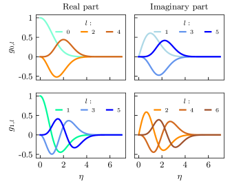
Figure 7: Coefficients $g_{sl}$ as a function of $\eta$ for different values of $s,l$. When $s=l$, the Laguerre polynomials are obtained.

In this section, we detail the derivation of the Peierls Hamiltonian in the photon basis. We first apply the Baker-Haussdorf-Campbell identity for non-commuting operators $A$ and $B$: $e^{A+B}=e^{-[A,B]/2}e^{A}e^{B}$, to the Peierls operator:

$$e^{i\eta_{ji}(d^{\dagger}+d)}=e^{-\eta^{2}_{ji}/2}e^{i\eta_{ji}d^{\dagger}}e^{i\eta_{ji}d},$$ (21)

This allows us to factor and re-organize the different powers of the creation and annihilation operators, which now are weighted by an additional exponential pre-factor $e^{-\eta^{2}_{ji}/2}$. Applied on the photonic number state $|n\rangle$, one gets

$$e^{i\eta_{ji}\left(d^{\dagger}+d\right)}|n\rangle=e^{-\eta_{ji}^{2}/2}\sum_{q,k=0}\Theta(q,n,k)|n-k+q\rangle$$ (22)

where we have defined

$$\Theta(q,n,k)=\frac{\left(i\eta\right)^{q+k}\sqrt{\left(n-k+q\right)!n!}}{q!k!\left(n-k\right)!}$$ (23)

where we have used the definitions of the creation/annihilation operators $d|n\rangle=\sqrt{n}|n-1\rangle$ and $d^{\dagger}|n\rangle=\sqrt{n+1}|n+1\rangle$. Then, for any two given photonic subspaces $l$ and $s$, the prefactors $g^{ji}_{ls}$ are:

$$g^{ji}_{ls}=\langle l|e^{i\eta_{ji}(d^{\dagger}+d)}|s\rangle=e^{-\eta^{2}_{ji}/2}\sum_{q=0}^{\infty}\sum_{k=0}^{s}\frac{(i\eta_{ji})^{q+k}}{q!k!(s-k)!}\sqrt{l!s!}$$ (24)

For $l=s$ (diagonal terms), this finite sum converges to the Laguerre polynomials $L_{s}$, and the off-diagonal terms are proportional to the Krummer’s confluent hypergeometric function ${}_{1}F_{1}(s,l,\eta^{2})$, as shown in the main text.

We now plot the analytical solution for the coefficients $g_{nn}=e^{-\eta^{2}/2}L_{n}(\eta^{2})$ and $g_{mn}=e^{-\eta_{ji}^{2}/2}\frac{\left(i\eta\right)^{n-m}}{\left(n-m\right)!}\sqrt{\frac{n!}{m!}}\,_{1}F_{1}(m,n,\eta^{2})$ as a function of the coupling (see Fig. 7).

While the Laguerre polynomials are purely real, the coefficients $g_{mn}$ are real or imaginary depending on the values for $n$ and $m$. This is shown in Fig. 7, where only the non-zero contribution has been plotted for each $n,m$.
Importantly, in the non-interacting limit $\eta\rightarrow 0$, the diagonal coefficients $g_{nn}\rightarrow 1$ go to one, while the off-diagonal ones $g_{mn}\rightarrow 0$: one-photon transitions disappear and we are left with the free fermionic Hamiltonian, as expected.
The oscillating behaviour of both $g_{nn}$ and $g_{mn}$ indicates the dominant subspaces will depend on the coupling strength considered, with a highly non-linear dependence.
Lastly, the dynamical localization prefactor $\mathrm{exp}(-\eta^{2}/2)$ ensures that all coefficients go to zero for large enough coupling strength, for all $n,m$.

Appendix C TRUNCATED HAMILTONIAN FOR LOW-PHOTON FREQUENCY AND COMPARISON WITH TAYLOR-EXPANDED HAMILTONIAN

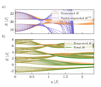
Figure 8: $a)$ Comparison of the energy spectrum of the truncated Hamiltonian and $H^{(2)}$, for $\Omega=10$, as a function of the coupling strength. $b)$ Comparison of the energy spectrum of the total Hamiltonian and the truncated one including only one-photon transitions, for a photon frequency lower than the bandwidth of the chain, $\Omega=3$, $J^{\prime}=1.5$, $J=1$, $r^{\prime}=0.4$, $n_{\mathrm{max}}=80$, $N=16$.

The total Hamiltonian in Eq. $(4)$ in the main text still is exact, and contains all orders of the vector potential, which are essential for maintaining gauge invariance for arbitrary coupling strength. In contrast, a naive Taylor expansion of the Peierls operator with the usual paramagnetic $\propto(d^{\dagger}+d)$ and diamagnetic $\propto(d^{\dagger}+d)^{2}$ terms would fail as the coupling strength increases towards the ultrastrong coupling regime [73, 74, 75]. The difference lies in the coefficients $g^{l,j}_{m,n}$, which are non-linear functions of $\eta_{l,j}$, and therefore the expansion in photonic Hubbard operators is unequivalent to that of a direct series expansion in powers of $\eta_{l,j}$.

Fig. 8$a)$ shows the energy spectrum for truncated Peierls Hamiltonian and the Taylor-expanded Hamiltonian to second order,

$$H^{(2)} = \sum_{\langle l,j\rangle}\left[J_{l,j}-\frac{\eta_{j,l}^{2}}{2}(d^{\dagger}+d)^{2}\right]c^{\dagger}_{l}c_{j}$$ (25)

$$+i(d^{\dagger}+d)\mathcal{J}$$

where $\mathcal{J}=\sum_{\langle l,j\rangle}\eta_{j,l}J_{l,j}(c^{\dagger}_{j}c_{l}-c^{\dagger}_{l}c_{j})$ contains a photon-dependent correction term to the hopping amplitudes. $H^{(2)}$ shows a good agreement for small coupling strength but differs radically from the Peierls Hamiltonian as the coupling increases. This is a consequence of the violation of gauge invariance. Accuracy would improve as higher orders of the photonic field are included [25].

Now, we test the validity of the truncated Hamiltonian far from the high frequency regime, when $\Omega$ is of the same order of magnitude as the fermionic bandwidth. Hence, mixed photonic bands are expected to appear in the energy spectrum, and the effect of higher photon transitions cannot be neglected for arbitrary coupling.

Fig. 8$b)$ shows the energy spectrum of the total $H$ and truncated one, for $\Omega=3$ and a bandwidth of $\Delta=5$. There is an overlap between different photonic bands, which becomes evident as the coupling is increased, resulting in a pattern of resonances and anticrossings. The truncated Hamiltonian reproduces the result of $H$ for small coupling strength with high accuracy, but as $\eta^{\prime}$ becomes larger, higher photon transitions are activated. Then, when the coupling becomes the dominant energy scale, both the exact and the truncated Hamiltonians yield the same result, as expected.

Appendix D EFFECT OF HIGHER-ORDER PHOTON TRANSITIONS IN THE ENERGY SPECTRUM

Figure 9: Comparison between different truncations of the total Hamiltonian (to one-, two-, and three-photon processes), as function of $\eta$ and for two cavity frequencies: $a)$ $\Omega=5$, and $b)$ $\Omega=10$. Parameters: $J^{\prime}=1.5,$, $J=1$, $N=8$, $n_{\mathrm{max}}=50$, $r^{\prime}=0.4$.

In this section, we explore the small, qualitative mismatch between the total Hamiltonian in Eq. $(4)$ and its truncated version, originated from the effect of higher-photon processes (two-photon, three-photon transitions…). There are two parameters that have an impact on this mismatch:

• The coupling strength: while for small values of the coupling strength the agreement between the truncated and the total Hamiltonian is perfect (see Fig. 1) in the main text, as the coupling strength increases and the system enters an ultrastrong coupling regime [76], higher-order photon transitions are expected to have a larger weight. With this, the mismatch between both Hamiltonians appears. Then, for very large values of the coupling, the two subsystems effective decouple and the differences are suppressed again, with both Hamiltonians correctly describing the system as a collection of degenerate bands separated by the cavity frequency. In fact, this is supported by Fig. $1$ in the SM, where we show the dependence of the functions $g_{m,n}$ with the coupling. Note that the off-diagonal functions $g_{m,n}$ with $m\neq n$ (controlling photon-exchange processes) are zero at $\eta=0$ and for large enough coupling strength, while reaching its highest value for intermediate values.

• The cavity frequency: For higher values of the cavity frequency, the photonic bands are further apart in energy and the exchange of photons becomes suppresses. However, as they come closer in the energy spectrum, higher-photon become more likely. This also implies that the effect of the breaking of chiral symmetry will be more evident in the energy spectrum for lower frequencies (i.e., in the assymetry of the bands).

$a)$ the coupling strength: as the coupling strength increases, higher-order photon transitions are expected to have a larger weight,
$b)$ the cavity frequency: for higher values of the cavity frequency, the photonic bands are further apart in energy and the exchange of photons becomes suppresses. However, as they come closer in the energy spectrum, higher-photon transitions become more likely.

Fig. 9 shows the energy spectrum from the total Hamiltonian, compared to its truncation version, and how this mismatch can be overcome by including higher-order photon transitions, in particular, two- and three-photon processes. Different choices of parameters are included. In panel $a)$, $\Omega=10$, which is the same choice as in the main text. We see how the truncated spectrums converge to the total one as more photon transitions are included. In panel $b)$, $\Omega=5$, and the convergence is worse, making it necessary to include more photon transitions. Note that in both cases, the disagreement is just qualitative: the truncated Hamiltonian to one-photon processes is enough to capture the relevant features of the interacting system. Besides, the mismatch depends on the coupling strength as well: it is negligable for small values of $\eta^{\prime}$, while it becomes larger in the ultrastrong regime.

Appendix E MEAN-FIELD HAMILTONIAN

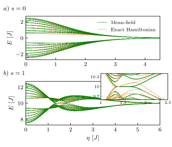
Figure 10: Comparison between the exact truncated (orange) and the mean-field fermionic Hamiltonian (green) as a function of the coupling strength $\eta^{\prime}$, for different photonic bands: $\mathbf{a)}$ $s=0$, and $\mathbf{b)}$ $s=1$. In $b)$, the inset shows the energy of the edge states vs. $\eta^{\prime}$, highlighting the difference between the chiral-symmetric MF spectrum and the truncated one in which chiral symmetry is broken. Parameters: $J^{\prime}=1.5$, $J=1$, $N=8$ unit cells, $n_{\mathrm{max}}=50$, $\Omega=10$, $r^{\prime}=0.4$.

We have shown that a simplified version of the gauge invariant Hamiltonian in the Coulomb gauge can be obtained by using disentangling techniques and truncating to one-photon processes. Now, we explore which features of the energy spectrum are retained when an even simpler approximation is used, i.e., a mean-field decoupling scheme in which each operator is rewritten as $\mathcal{O}=\langle\mathcal{O}\rangle+\delta\mathcal{O}$, separating its mean value $\langle\mathcal{O}\rangle$ from the contribution of quantum fluctuations $\delta\mathcal{O}$. At the MF level (linear terms in $\delta\mathcal{O}$), we obtain two effectively decoupled Hamiltonians for each subsystem, where the back-action due to the interaction is encoded in renormalized system parameters. An additional fluctuations Hamiltonian (second-order in $\delta\mathcal{O}$) encodes the role of quantum fluctuations, introducing correlations between subsystems. A MF analysis of the problem allows to identify which features are captured by the photo-dressing of the fermionic system and which of them are linked to electron-photon correlations. In the following, the MF approach will be used on the truncated version of the exact Hamiltonian.

For the photonic field, the MF decoupling on the truncated Hamiltonian gives a particularly simple description: the resulting Hamiltonian is diagonal in the basis of Hubbard operators $Y^{nn}$. First, let us define the following fermionic operators, which contain the energy contribution of both the inter- and intra-dimer hopping

$$f^{\prime}_{+}=t^{\prime}\sum_{\alpha}a^{\dagger}_{\alpha}b_{\alpha}=(f^{\prime}_{-})^{\dagger},\hskip 10.0ptf_{+}=t\sum_{\alpha}b^{\dagger}_{\alpha}a_{\alpha+1}=(f_{-})^{\dagger},$$ (26)

together with $f^{(\prime)}=f^{(\prime)}_{+}+f^{(\prime)}_{-}$. Then, the MF photonic Hamiltonian can be readily written as

$$H_{\text{MF,phot}}=\sum_{n}\bigg{\{}n\Omega+\langle f^{\prime}\rangle g^{\prime}_{nn}+\langle f\rangle g_{nn}\bigg{\}}Y^{nn}.$$ (27)

Note that one-photon transitions are absent in the MF photonic Hamiltonian $H_{\text{MF,phot}}$, which is diagonal in the photonic operators. This is due to the symmetry of the truncated Peierls operator in Eq. $(2)$ (main text) and the form of the off-diagonal coefficients $g^{(\prime),\pm}_{n,n+1}$. In general, the creation/annihilation of $m$ photons in the system through the operators $Y^{n+m,n}$/$Y^{n,n+m}$ is linked to the electronic inter- and intra-dimer hopping, where the corresponding tunneling amplitudes are weighted by the prefactors $g^{(\prime),\pm}_{n,n+m}$. For the case of one-photon transitions, the direction of the hopping (to the left, $\eta^{(\prime)}>0$, or to the right, $\eta^{(\prime)}<0$) has the effect of adding an extra sign to $g^{(\prime),\pm}_{n,n+1}$, so that they finally cancel out in $H_{\mathrm{MF,phot}}$. Note that for arbitrary $m$, all odd-photon transitions ($m=1,3,5,...$) would be absent from the MF Hamiltonian, while even ones ($m=2,4,6,...$) are not cancelled out. This is agreement with Ref. [16].

Then, the eigenstates of $H_{\text{MF,phot}}$ in Eq. (27) can be labelled with the photon number $n=0,1,2,...$, being $n=0$ the ground state with zero photons. This means that the different photonic subspaces will not hybridize for large coupling strength, and the number of photons in the system is constant in time.

The Hamiltonian in Eq. (27) indicates that the interaction with the fermionic system shifts the energy of the cavity photons, which depends on the fermionic state through $\langle f^{(\prime)}\rangle=\mathrm{Tr}\{\rho_{\text{MF,fer}}f^{(\prime)}\}$. Being absent in the classical regime, the frequency shift is crucial in cavity QED set-ups for quantum non-demolition measurements on the fermionic system using the photonic radiated signal [77, 78, 79, 80].

For the fermionic system, the MF decoupling yields an unperturbed SSH Hamiltonian with renormalized hopping amplitudes due to the interaction with the photonic field,

$$t^{(\prime)}\rightarrow\tilde{t}^{(\prime)}=t^{(\prime)}g^{(\prime)}_{s,s}=t^{(\prime)}e^{-\eta^{(\prime)2}/2}L_{s}\left(\eta^{(\prime)2}\right).$$ (28)

Note that both $\tilde{t}^{\prime}$ and $\tilde{t}$ inherit the dynamical localization prefactors that ensures the suppression of the hopping at large coupling strength, while the dependence on the Laguerre polynomial $L_{s}(\eta^{(\prime)2})$ gives an oscillatory dependence with $\eta^{\prime}$. Here we have assumed that the cavity is prepared with a fixed number of photons, $\rho_{\text{MF,phot}}=|s\rangle\langle s|$.

Fig. 10 shows the MF fermionic energy spectrum compared with the exact truncated Hamiltonian. The former reproduces the topological phase transitions as a function of the coupling strength, which indicates that topology is controlled by the dressing of the fermionic degrees of freedom (first term in Eq. $(4)$ of the main text) and the ratio of the renormalized hoppings $\tilde{t}^{\prime}/\tilde{t}$.

Appendix F CALCULATION OF THE TOPOLOGICAL INVARIANT FOR THE INTERACTING SYSTEM

An analytical solution for $G^{m,m}_{\alpha,\beta}(\omega,k)$ can be found by writing its equation of motion (EOM) in time domain

$$i\frac{dG^{m,m}_{\alpha,\beta}(t,k)}{dt} = \delta(t)\left\{\alpha_{k}Y^{m,m}(t),\beta^{\dagger}_{k}\right\}$$ (29)

$$-i\theta(t)\langle\left\{\left[\alpha^{\dagger}_{k}Y^{m,m},H(k)\right],\beta^{\dagger}_{k}\right\}\rangle.$$

$H(k)$ is the k-space Hamiltonian of the interacting system, obtained from Fourier transforming the fermionic creation/annihilation operators into $k-$space. Its truncated version to one-photon processes is

$$H(k) = \sum_{n}n\Omega Y^{n,n}$$ (30)

$$+\sum_{n}\left\{h_{n}(k)a_{k}^{\dagger}b_{k}+h^{*}_{n}(k)b_{k}^{\dagger}a_{k}\right\}Y^{nn}$$

$$+\sum_{n}\left\{\bar{h}_{n}(k)a_{k}^{\dagger}b_{k}+\bar{h}^{*}_{n}(k)b_{k}^{\dagger}a_{k}\right\}\cdot$$

$$\hskip 20.0pt\cdot\left(Y^{n+1,n}+Y^{n,n+1}\right)$$

together with the definitions

$$h_{n}(k) = t^{\prime}g_{nn}^{\prime}+tg_{nn}e^{ik}$$ (31)

$$\bar{h}_{n}(k) = t^{\prime}g_{n+1,n}^{+\prime}+te^{ik}g_{n+1,n}^{-}.$$ (32)

To solve Eq. 29 we have considered single occupation for the SSH chain, which greatly simplifies the fermionic algebra. Second, with the truncation of $\mathcal{H}(k)$, the EOM can be restricted to those terms involving only one-photon transitions, namely $G^{m\pm 1,m}_{\alpha,\beta}(k,\omega)$ and $G^{m,m\pm 1}_{\alpha,\beta}(k,\omega)$. This entails a major reduction of the equations and enables the solution of the system, that would otherwise involve infinitely many GFs of the form $G^{m,m+l}_{\alpha,\beta}$ and $G^{m+l,m}_{\alpha,\beta}$ ($l=1,2,...$). With all this, and neglecting off-diagonal couplings, the solution for $G^{m,m}_{\alpha,\beta}(k,\omega)$ can be written in the form

$$G^{m,m}(k,\omega)=\frac{\langle Y^{m,m}\rangle}{2\pi}\left[F^{m,m}(k,\omega)\right]^{-1},$$ (33)

where $F^{m,m}$ is a $2\times 2$ matrix which contains the pole structure for $G^{m,m}(k,\omega)$. By defining $\varepsilon^{2}_{m}(k)=h_{m}(k)\hskip 1.0pth^{*}_{m}(k)$ and $\bar{\varepsilon}^{2}_{m}(k)=\bar{h}_{m}(k)\hskip 1.0pt\bar{h}^{*}_{m}(k)$, we can write the following expression for the matrix elements of $F^{m,m}$,

$$F^{m,m}_{A,A}(k,\omega) = \omega-\frac{\bar{\varepsilon}^{2}_{m}(k)[\omega+\Omega]}{p^{+}_{m+1}(\omega,k)}$$ (34)

$$\hskip 50.0pt-\frac{\bar{\varepsilon}_{m-1}(k)[\omega-\Omega]}{p^{-}_{m-1}(\omega,k)},$$

$$F^{m,m}_{A,B}(k,\omega) = -h_{m}(k)-\frac{\bar{h}_{m}^{2}(k)h_{m+1}^{*}(k)}{p^{+}_{m+1}(\omega,k)}$$ (35)

$$\hskip 50.0pt-\frac{\bar{h}^{2}_{m-1}(k)h^{*}_{m-1}(k)}{p^{-}_{m-1}(\omega,k)},$$

$$F^{m,m}_{B,A}(k,\omega) = \left[F^{m,m}_{A,B}(k,\omega)\right]^{*},$$ (36)

$$\hskip 10.0ptF_{B,B}^{m,m}(k,\omega)=F_{A,A}^{m,m}(k,\omega),$$

with $p^{+}_{m}(k,\omega)=(\omega+\Omega)^{2}-\varepsilon^{2}_{m}(k)$ and $p^{-}_{s}(k,\omega)=(\omega-\Omega)^{2}-\varepsilon^{2}_{m}(k)$.

The first term in Eqs. (34) and (35) accounts for the mean-field result of dressed electrons, while the second and third terms contain the contribution of one-photon transitions, which allows us to interprete the implications for the topology of fermionic chain. Note that those terms contain additional poles with mixed light-matter resonances, due to the presence of correlations between subsystems.

Physically, the additional terms in $F^{m,m}_{\alpha,\alpha}(k,\omega)$ indicate the transfer of spectral weight to the subspaces of $(m+1)-$ (second term in Eq. (34) and $(m-1)-$photons (third term in Eq. (34). Interestingly, since $\varepsilon^{2}_{m}(k)\neq\varepsilon^{2}_{m-1}(k)$, the transfer of spectral weight is not symmetric. Therefore, the exchange of one-photon from a given photonic band with the upper/lower bands are not equivalent.

Appendix G SPECTRAL FUNCTION FOR A NON-EMPTY CAVITY

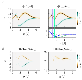
Figure 11: Spectral function $D_{\mathrm{MF}}$ and $D_{\mathrm{e}}$ for $n=1$ as a function of $\eta$ and $\omega$. The fermionic system is prepared in the ground state for a trivial chain. Panel $a)$ shows the renormalization of the cavity frequency and the appearance of additional excitations, while the bottom panel indicates the connection between the abrupt changes in the poles and the hopping renormalization. Panel $b)$ shows additional light-matter resonances that appear in $D_{\mathrm{e}}$ and that are absent in the MF solution, $J^{\prime}=1.5$, $J=1$, $r^{\prime}=0.4$, $\Omega=10$, $n_{\mathrm{max}}=70$, $N=16$.

Let us now consider a different state preparation with a non-empty cavity, with $n=1$ photons, which is depicted in Fig. 11. Panel $a)$ shows the comparison between the MF and the exact result, $D_{\mathrm{MF}}(\omega)$ and $D_{\mathrm{e}}(\omega)$, respectively. While the photon frequency is shifted as a function of the coupling as in the empty case, there are extra effects that are missing in Fig. $2$ in the main text ($n=0$): the appearance of an additional pole for $\eta>0$. This behaviour is well-reproduced by $D_{\mathrm{MF}}(\omega)$, which indicates that the two poles correspond to the exchange of virtual photons with the upper $(n+1)$ and the lower photonic band $(n-1)$, and are not caused by electron-photon correlations (this is also consistent with the fact that for the zeroth photonic band $n=0$ there is only one pole in the photonic spectral function). Since each band renormalizes differently, the exchange of photons with the upper and lower band are not equivalent processes, and therefore the corresponding poles have their own dependence on $\omega$ and $\eta^{\prime}$. For large $\eta^{\prime}$, they both suppress to zero, as for the empty cavity.

There is an additional feature in Fig. 11 that is also missing Fig. $2$ (main text), and that appears in both the MF and the exact calculation: the presence of abrupt changes in the poles, which are related to the hopping renormalization as a function of $\eta^{\prime}$. This can be easily connected with the dressing of the hopping amplitudes and how they change as a function of $\eta^{\prime}$. The oscillation of the Laguerre polynomials with $\eta^{\prime}$ for the non-empty cavity implies that the hopping amplitudes will be effectively suppressed at certain values of the coupling strength, with the subsequent change of sign. While the topology of the chain is determined by the absolute value of the ratio between $t^{\prime}g^{\prime}_{nn}$ and $tg_{nn}$, these changes in the hopping amplitudes are also reflected in the photonic spectral function.

Lastly, panel $b)$ shows additional light-matter resonances that appear in the exact spectral function and that are absent in the MF solution.

Appendix H ADDITIONAL RESULTS FOR STATE TRANSFER DYNAMICS

In this section we provide with additional numerical results regarding the transfer dynamics, and how the parameters of the hybrid system can be fined tuned to change the transfer time. As shown in the main text, the value of the light-matter coupling can drastically change the dynamics of a charge in the SSH chain, specially if the system undergoes a topological phase transition. For the topological phase, the presence of edge states induces Rabi oscillations between the ending sites of the chain, for an appropriate fermionic state preparation (i.e., the particle occupies the ending site of the chain at $t=0$). The value of the coupling strength can be further tuned to control the energy splitting of the edge states, and therefore the period of the oscillations [66]. This is what we show in Fig. 12, $a)$ panel, where a slight change in $\eta$ reduces the frequency of the oscillation. Importantly, for this case we consider $n=2$ photons in the cavity.

Similarly, an additional degree of freedom to control transfer dynamics is the cavity state preparation. For $n=3$ photons, we can also find values of $\eta$ for which the system displays edge states (although the unperturbed hopping amplitudes are chosen such that the chain is trivial). The corresponding charge dynamics are shown in Fig. 12, $b)$ panel. Not only the number of photons affects the band structure and, therefore, the splitting of the edge states, but we can also simultaneously tune the coupling strength to find desired transfer periods.

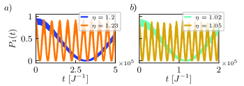
Figure 12: Fermionic occupation probability of the first site $P_{1}(t)$, as a function of time, for different coupling strengths $\eta$ and photonic subspaces: $a)$ $n=2$, and $b)$ $n=3$, showing that both parameters can be used to control the oscillation frequency. The system is prepared such that the the particle occupies the first site of the chain at $t=0$. $J^{\prime}=1.5,J=1,r^{\prime}=0.4,N=16,\Omega=10,nmax=50$.

References

- Grossmann et al. [1991] F. Grossmann, T. Dittrich, P. Jung, and P. Hänggi, Coherent destruction of tunneling, Phys. Rev. Lett. 67, 516 (1991).
- Lindner et al. [2011] N. H. Lindner, G. Refael, and V. Galitski, Floquet topological insulator in semiconductor quantum wells, Nature Physics 7, 490 (2011).
- Gómez-León and Platero [2013] A. Gómez-León and G. Platero, Floquet-bloch theory and topology in periodically driven lattices, Phys. Rev. Lett. 110, 200403 (2013).
- Gómez-León et al. [2014] A. Gómez-León, P. Delplace, and G. Platero, Engineering anomalous quantum hall plateaus and antichiral states with ac fields, Phys. Rev. B 89, 205408 (2014).
- Benito et al. [2014] M. Benito, A. Gómez-León, V. M. Bastidas, T. Brandes, and G. Platero, Floquet engineering of long-range -wave superconductivity, Phys. Rev. B 90, 205127 (2014).
- Grushin et al. [2014] A. G. Grushin, A. Gómez-León, and T. Neupert, Floquet fractional chern insulators, Phys. Rev. Lett. 112, 156801 (2014).
- Díaz-Fernández et al. [2019] A. Díaz-Fernández, E. Díaz, A. Gómez-León, G. Platero, and F. Domínguez-Adame, Floquet engineering of dirac cones on the surface of a topological insulator, Phys. Rev. B 100, 075412 (2019).
- Rudner and Lindner [2020] M. S. Rudner and N. H. Lindner, Band structure engineering and non-equilibrium dynamics in floquet topological insulators, Nature Reviews Physics 2, 229 (2020).
- Oka and Kitamura [2019] T. Oka and S. Kitamura, Floquet engineering of quantum materials, Annual Review of Condensed Matter Physics 10, 387 (2019), https://doi.org/10.1146/annurev-conmatphys-031218-013423 .
- Aguado and Platero [1997] R. Aguado and G. Platero, Dynamical localization and absolute negative conductance in an ac-driven double quantum well, Phys. Rev. B 55, 12860 (1997).
- Platero and Aguado [2004] G. Platero and R. Aguado, Photon-assisted transport in semiconductor nanostructures, Physics Reports 395, 1 (2004).
- Engelhardt et al. [2016] G. Engelhardt, M. Benito, G. Platero, and T. Brandes, Topological instabilities in ac-driven bosonic systems, Phys. Rev. Lett. 117, 045302 (2016).
- Creffield and Platero [2010] C. E. Creffield and G. Platero, Coherent control of interacting particles using dynamical and aharonov-bohm phases, Phys. Rev. Lett. 105, 086804 (2010).
- Higashikawa et al. [2018] S. Higashikawa, H. Fujita, and M. Sato, Floquet engineering of classical systems, arXiv: Strongly Correlated Electrons (2018).
- Sentef et al. [2020a] M. A. Sentef, J. Li, F. Künzel, and M. Eckstein, Quantum to classical crossover of floquet engineering in correlated quantum systems, Phys. Rev. Research 2, 033033 (2020a).
- Dmytruk and Schiro [2022] O. Dmytruk and M. Schiro, Controlling topological phases of matter with quantum light, Communications Physics 5, 271 (2022).
- Li et al. [2020] J. Li, D. Golez, G. Mazza, A. J. Millis, A. Georges, and M. Eckstein, Electromagnetic coupling in tight-binding models for strongly correlated light and matter, Phys. Rev. B 101, 205140 (2020).
- Li et al. [2022] J. Li, L. Schamriß, and M. Eckstein, Effective theory of lattice electrons strongly coupled to quantum electromagnetic fields, Phys. Rev. B 105, 165121 (2022).
- Eckhardt et al. [2022] C. J. Eckhardt, G. Passetti, M. Othman, C. Karrasch, F. Cavaliere, M. A. Sentef, and D. M. Kennes, Quantum floquet engineering with an exactly solvable tight-binding chain in a cavity, Communications Physics 5, 122 (2022).
- Schlawin et al. [2022] F. Schlawin, D. M. Kennes, and M. A. Sentef, Cavity quantum materials, Applied Physics Reviews 9, 011312 (2022), https://pubs.aip.org/aip/apr/article-pdf/doi/10.1063/5.0083825/16648467/011312_1_online.pdf .
- Hübener et al. [2021] H. Hübener, U. De Giovannini, C. Schäfer, J. Andberger, M. Ruggenthaler, J. Faist, and A. Rubio, Engineering quantum materials with chiral optical cavities, Nature Materials 20, 438 (2021).
- Bloch et al. [2022] J. Bloch, A. Cavalleri, V. Galitski, M. Hafezi, and A. Rubio, Strongly correlated electron–photon systems, Nature 606, 41 (2022).
- Passetti et al. [2023] G. Passetti, C. J. Eckhardt, M. A. Sentef, and D. M. Kennes, Cavity light-matter entanglement through quantum fluctuations, Phys. Rev. Lett. 131, 023601 (2023).
- Eckardt and Anisimovas [2015a] A. Eckardt and E. Anisimovas, High-frequency approximation for periodically driven quantum systems from a floquet-space perspective, New Journal of Physics 17, 093039 (2015a).
- Di Stefano et al. [2019] O. Di Stefano, A. Settineri, V. Macrì, L. Garziano, R. Stassi, S. Savasta, and F. Nori, Resolution of gauge ambiguities in ultrastrong-coupling cavity quantum electrodynamics, Nature Physics 15, 803 (2019).
- Settineri et al. [2021] A. Settineri, O. Di Stefano, D. Zueco, S. Hughes, S. Savasta, and F. Nori, Gauge freedom, quantum measurements, and time-dependent interactions in cavity qed, Phys. Rev. Research 3, 023079 (2021).
- Savasta et al. [2021] S. Savasta, O. Di Stefano, A. Settineri, D. Zueco, S. Hughes, and F. Nori, Gauge principle and gauge invariance in two-level systems, Phys. Rev. A 103, 053703 (2021).
- Garziano et al. [2020] L. Garziano, A. Settineri, O. Di Stefano, S. Savasta, and F. Nori, Gauge invariance of the dicke and hopfield models, Phys. Rev. A 102, 023718 (2020).
- Li and Eckstein [2020] J. Li and M. Eckstein, Manipulating intertwined orders in solids with quantum light, Phys. Rev. Lett. 125, 217402 (2020).
- D’Alessio and Rigol [2014] L. D’Alessio and M. Rigol, Long-time behavior of isolated periodically driven interacting lattice systems, Phys. Rev. X 4, 041048 (2014).
- Bukov et al. [2016] M. Bukov, M. Heyl, D. A. Huse, and A. Polkovnikov, Heating and many-body resonances in a periodically driven two-band system, Phys. Rev. B 93, 155132 (2016).
- Weidinger and Knap [2017] S. A. Weidinger and M. Knap, Floquet prethermalization and regimes of heating in a periodically driven, interacting quantum system, Scientific Reports 7, 45382 (2017).
- Ponte et al. [2015] P. Ponte, Z. Papić, F. Huveneers, and D. A. Abanin, Many-body localization in periodically driven systems, Phys. Rev. Lett. 114, 140401 (2015).
- Zhang et al. [2016] L. Zhang, V. Khemani, and D. A. Huse, A floquet model for the many-body localization transition, Phys. Rev. B 94, 224202 (2016).
- Iwahori and Kawakami [2017] K. Iwahori and N. Kawakami, Stabilization of prethermal floquet steady states in a periodically driven dissipative bose-hubbard model, Phys. Rev. A 95, 043621 (2017).
- McIver et al. [2020] J. W. McIver, B. Schulte, F.-U. Stein, T. Matsuyama, G. Jotzu, G. Meier, and A. Cavalleri, Light-induced anomalous hall effect in graphene, Nature Physics 16, 38 (2020).
- Pérez-González et al. [2019a] B. Pérez-González, M. Bello, G. Platero, and A. Gómez-León, Simulation of 1d topological phases in driven quantum dot arrays, Phys. Rev. Lett. 123, 126401 (2019a).
- Delplace et al. [2013] P. Delplace, A. Gómez-León, and G. Platero, Merging of dirac points and floquet topological transitions in ac-driven graphene, Phys. Rev. B 88, 245422 (2013).
- Rudner et al. [2013] M. S. Rudner, N. H. Lindner, E. Berg, and M. Levin, Anomalous edge states and the bulk-edge correspondence for periodically driven two-dimensional systems, Phys. Rev. X 3, 031005 (2013).
- Quelle et al. [2017] A. Quelle, C. Weitenberg, K. Sengstock, and C. Morais Smith, Driving protocol for a floquet topological phase without static counterpart, New Journal of Physics 19, 113010 (2017).
- Nathan et al. [2019] F. Nathan, D. Abanin, E. Berg, N. H. Lindner, and M. S. Rudner, Anomalous floquet insulators, Phys. Rev. B 99, 195133 (2019).
- Roy and Harper [2017] R. Roy and F. Harper, Periodic table for floquet topological insulators, Phys. Rev. B 96, 155118 (2017).
- Su et al. [1979] W. P. Su, J. R. Schrieffer, and A. J. Heeger, Solitons in polyacetylene, Phys. Rev. Lett. 42, 1698 (1979).
- Heeger et al. [1988] A. J. Heeger, S. Kivelson, J. R. Schrieffer, and W. P. Su, Solitons in conducting polymers, Rev. Mod. Phys. 60, 781 (1988).
- Appugliese et al. [2022] F. Appugliese, J. Enkner, G. L. Paravicini-Bagliani, M. Beck, C. Reichl, W. Wegscheider, G. Scalari, C. Ciuti, and J. Faist, Breakdown of topological protection by cavity vacuum fields in the integer quantum hall effect, Science 375, 1030 (2022), https://www.science.org/doi/pdf/10.1126/science.abl5818 .
- Dmytruk and Schiró [2021] O. Dmytruk and M. Schiró, Gauge fixing for strongly correlated electrons coupled to quantum light, Phys. Rev. B 103, 075131 (2021).
- Chiu et al. [2016] C.-K. Chiu, J. C. Y. Teo, A. P. Schnyder, and S. Ryu, Classification of topological quantum matter with symmetries, Rev. Mod. Phys. 88, 035005 (2016).
- Schnyder et al. [2008] A. P. Schnyder, S. Ryu, A. Furusaki, and A. W. W. Ludwig, Classification of topological insulators and superconductors in three spatial dimensions, Phys. Rev. B 78, 195125 (2008).
- Pérez-González et al. [2019b] B. Pérez-González, M. Bello, A. Gómez-León, and G. Platero, Interplay between long-range hopping and disorder in topological systems, Phys. Rev. B 99, 035146 (2019b).
- Eckardt and Anisimovas [2015b] A. Eckardt and E. Anisimovas, High-frequency approximation for periodically driven quantum systems from a floquet-space perspective, New Journal of Physics 17, 093039 (2015b).
- Asbóth et al. [2016] J. K. Asbóth, L. Oroszlány, and A. Pályi, A Short Course on Topological Insulators (Springer Cham, New York, 2016).
- Hatsugai [1993] Y. Hatsugai, Chern number and edge states in the integer quantum hall effect, Phys. Rev. Lett. 71, 3697 (1993).
- Gurarie [2011] V. Gurarie, Single-particle green’s functions and interacting topological insulators, Phys. Rev. B 83, 085426 (2011).
- Essin and Gurarie [2011] A. M. Essin and V. Gurarie, Bulk-boundary correspondence of topological insulators from their respective green’s functions, Phys. Rev. B 84, 125132 (2011).
- Manmana et al. [2012] S. R. Manmana, A. M. Essin, R. M. Noack, and V. Gurarie, Topological invariants and interacting one-dimensional fermionic systems, Phys. Rev. B 86, 205119 (2012).
- Shiozaki et al. [2018] K. Shiozaki, H. Shapourian, K. Gomi, and S. Ryu, Many-body topological invariants for fermionic short-range entangled topological phases protected by antiunitary symmetries, Phys. Rev. B 98, 035151 (2018).
- Shapourian et al. [2017] H. Shapourian, K. Shiozaki, and S. Ryu, Many-body topological invariants for fermionic symmetry-protected topological phases, Phys. Rev. Lett. 118, 216402 (2017).
- Schäfer et al. [2020] C. Schäfer, M. Ruggenthaler, V. Rokaj, and A. Rubio, Relevance of the quadratic diamagnetic and self-polarization terms in cavity quantum electrodynamics, ACS Photonics 7, 975 (2020).
- Blais et al. [2004a] A. Blais, R.-S. Huang, A. Wallraff, S. M. Girvin, and R. J. Schoelkopf, Cavity quantum electrodynamics for superconducting electrical circuits: An architecture for quantum computation, Phys. Rev. A 69, 062320 (2004a).
- Lupaşcu et al. [2007] A. Lupaşcu, S. Saito, T. Picot, P. C. de Groot, C. J. P. M. Harmans, and J. E. Mooij, Quantum non-demolition measurement of a superconducting two-level system, Nature Physics 3, 119 (2007).
- Nakajima et al. [2019] T. Nakajima, A. Noiri, J. Yoneda, M. R. Delbecq, P. Stano, T. Otsuka, K. Takeda, S. Amaha, G. Allison, K. Kawasaki, A. Ludwig, A. D. Wieck, D. Loss, and S. Tarucha, Quantum non-demolition measurement of an electron spin qubit, Nature Nanotechnology 14, 555 (2019).
- Gómez-León et al. [2022] A. Gómez-León, F. Luis, and D. Zueco, Dispersive readout of molecular spin qudits, Phys. Rev. Applied 17, 064030 (2022).
- Pérez-González et al. [2022] B. Pérez-González, A. Gómez-León, and G. Platero, Topology detection in cavity qed, Phys. Chem. Chem. Phys. 24, 15860 (2022).
- Leijnse and Flensberg [2011] M. Leijnse and K. Flensberg, Quantum information transfer between topological and spin qubit systems, Phys. Rev. Lett. 107, 210502 (2011).
- Nicolai and Büchler [2017] L. Nicolai and H. P. Büchler, Topological networks for quantum communication between distant qubits, npj Quantum Information 3, 47 (2017).
- Bello et al. [2016] M. Bello, C. E. Creffield, and G. Platero, Long-range doublon transfer in a dimer chain induced by topology and ac fields, Scientific Reports 6, 22562 (2016).
- Bello et al. [2017] M. Bello, C. E. Creffield, and G. Platero, Sublattice dynamics and quantum state transfer of doublons in two-dimensional lattices, Phys. Rev. B 95, 094303 (2017).
- Kibis et al. [2011] O. V. Kibis, O. Kyriienko, and I. A. Shelykh, Band gap in graphene induced by vacuum fluctuations, Phys. Rev. B 84, 195413 (2011).
- Wang et al. [2019] X. Wang, E. Ronca, and M. A. Sentef, Cavity quantum electrodynamical chern insulator: Towards light-induced quantized anomalous hall effect in graphene, Phys. Rev. B 99, 235156 (2019).
- Dartiailh et al. [2017] M. C. Dartiailh, T. Kontos, B. Douçot, and A. Cottet, Direct cavity detection of majorana pairs, Phys. Rev. Lett. 118, 126803 (2017).
- Dmytruk and Trif [2023] O. Dmytruk and M. Trif, Microwave detection of gliding majorana zero modes in nanowires, Phys. Rev. B 107, 115418 (2023).
- Trif and Tserkovnyak [2012] M. Trif and Y. Tserkovnyak, Resonantly tunable majorana polariton in a microwave cavity, Phys. Rev. Lett. 109, 257002 (2012).
- Kiffner et al. [2019] M. Kiffner, J. R. Coulthard, F. Schlawin, A. Ardavan, and D. Jaksch, Manipulating quantum materials with quantum light, Phys. Rev. B 99, 085116 (2019).
- Andolina et al. [2019] G. M. Andolina, F. M. D. Pellegrino, V. Giovannetti, A. H. MacDonald, and M. Polini, Cavity quantum electrodynamics of strongly correlated electron systems: A no-go theorem for photon condensation, Phys. Rev. B 100, 121109 (2019).
- Sentef et al. [2020b] M. A. Sentef, J. Li, F. Künzel, and M. Eckstein, Quantum to classical crossover of floquet engineering in correlated quantum systems, Phys. Rev. Research 2, 033033 (2020b).
- Frisk Kockum et al. [2019] A. Frisk Kockum, A. Miranowicz, S. De Liberato, S. Savasta, and F. Nori, Ultrastrong coupling between light and matter, Nature Reviews Physics 1, 19 (2019).
- Blais et al. [2004b] A. Blais, R.-S. Huang, A. Wallraff, S. M. Girvin, and R. J. Schoelkopf, Cavity quantum electrodynamics for superconducting electrical circuits: An architecture for quantum computation, Phys. Rev. A 69, 062320 (2004b).
- Wallraff et al. [2005] A. Wallraff, D. I. Schuster, A. Blais, L. Frunzio, J. Majer, M. H. Devoret, S. M. Girvin, and R. J. Schoelkopf, Approaching unit visibility for control of a superconducting qubit with dispersive readout, Phys. Rev. Lett. 95, 060501 (2005).
- Boissonneault et al. [2009] M. Boissonneault, J. M. Gambetta, and A. Blais, Dispersive regime of circuit qed: Photon-dependent qubit dephasing and relaxation rates, Phys. Rev. A 79, 013819 (2009).
- Gambetta et al. [2006] J. Gambetta, A. Blais, D. I. Schuster, A. Wallraff, L. Frunzio, J. Majer, M. H. Devoret, S. M. Girvin, and R. J. Schoelkopf, Qubit-photon interactions in a cavity: Measurement-induced dephasing and number splitting, Phys. Rev. A 74, 042318 (2006).