Beyond Moments: Robustly Learning Affine Transformations with Asymptotically Optimal Error

Abstract

We present a polynomial-time algorithm for robustly learning an unknown affine transformation of the standard hypercube from samples, an important and well-studied setting for independent component analysis (ICA). Specifically, given an $\varepsilon$-corrupted sample from a distribution $D$ obtained by applying an unknown affine transformation $x\rightarrow Ax+s$ to the uniform distribution on a $d$-dimensional hypercube $[-1,1]^{d}$, our algorithm constructs $\hat{A},\hat{s}$ such that the total variation distance of the distribution $\hat{D}$ from $D$ is $O(\varepsilon)$ using poly$(d)$ time and samples. Total variation distance is the information-theoretically strongest possible notion of distance in our setting and our recovery guarantees in this distance are optimal up to the absolute constant factor multiplying $\varepsilon$. In particular, if the columns of $A$ are normalized to be unit length, our total variation distance guarantee implies a bound on the sum of the $\ell_{\_}2$ distances between the column vectors of $A$ and $A^{\prime}$, $\sum_{\_}{i=1}^{d}\lVert a_{\_}i-\hat{a}_{\_}i\rVert_{\_}2=O(\varepsilon)$. In contrast, the strongest known prior results only yield a $\varepsilon^{O(1)}$ (relative) bound on the distance between individual $a_{\_}i$’s and their estimates and translate into an $O(d\varepsilon)$ bound on the total variation distance.

Prior algorithms for this problem rely on implementing standard approaches [7] for ICA based on the classical method of moments [12, 19] combined with robust moment estimators. We observe that an approach based on $o(\log d)$-degree moments provably fails to obtain non-trivial total variation distance guarantees for robustly learning an affine transformation unless $\varepsilon<1/d^{O(1)}$. Our key innovation is a new approach to ICA (even to outlier-free ICA) that circumvents the difficulties in the classical method of moments and instead relies on a new geometric certificate of correctness of an affine transformation. Our algorithm is based on a new method that iteratively improves an estimate of the unknown affine transformation whenever the requirements of the certificate are not met.

1 Introduction

We consider the problem of learning affine transformations from samples. Specifically, we are given i.i.d. points $x\in{\mathbb R}^{d}$ obtained after applying an unknown affine transformation to a uniform sample from the hypercube $[-1,1]^{d}$, i.e., $x=As+a$ where $a,A$ are unknown and each coordinate of $s$ is uniformly sampled in $[-1,1]$. The study of efficient algorithms for estimating the unknown affine transformation up to desired error is a major topic in signal processing [7, 9, 10], with many interesting algorithms and heuristics. It is often called standard ICA (a special case of the well-studied Independent Component Analysis) or blind deconvolution or the “cocktail party" problem.

Algorithms for recovering the unknown affine transformation $A$ are generally based on higher directional moments of the distribution. The empirical mean and covariance of the transformed samples can be used to find an affine transformation that matches the mean and second moments of the original cube. The correct rotation can be identified by first making the distrbution isotropic (zero mean, identity covariance) and then examining the fourth moment of the empirical distribution. The directions that maximize the fourth moment correspond to the facet normals of the correct rotation, see e.g.,  [12, 19]. The “method of moments" has been extended, using higher moments, to various generalizations of standard ICA, including more general product distributions and underdetermined ICA [13].

While the model has been quite influential and is widely studied, it is reasonable to expect that data will contain errors and will deviate, at least slightly, from the precise model. Recovering the underlying model parameters despite corruption, even arbitrary adversarial noise, is the mainstay of robust statistics, a field that has enjoyed a renaissance over the past decade (and is now called Algorithmic Robust Statistics). Beginning with the robust estimation of the mean of high-dimensional distributions [11, 17], there has been tremendous progress on a variety of well-known and central problems in statistical learning theory, including linear regression [14, 3]  covariance estimation [8] and Gaussian mixture models [2]. In all these cases, nearly optimal guarantees are known, asymptotically matching statistical lower bounds for the error of the estimated parameters.

Despite much progress on ICA and on robust estimation, the robust version of the problem has thus far evaded solution. The precise problem is as follows: we are given samples from an unknown affine transformation of a cube, after an $\varepsilon$ fraction of the sample has been arbitrarily (adversarially) corrupted; estimate the affine transformation. Information-theoretically, it is possible to estimate an affine transformation so that the resulting distribution is within TV distance $O(\varepsilon)$ of the unknown transformation. But can we find this algorithmically?

Prior works [17, 16] obtained some guarantees for ICA in the presence of adversarial outliers by applying robust estimators for moments of data into the classical ICA algorithms based on the method of moments. The resulting guarantees allow recovering a linear transformation $\hat{A}$ so that (up to a permutation) each column of $\hat{A}$ is close to the corresponding column of $A$ up to $(1\pm\varepsilon^{O(1)})$ relative error in $\ell_{\_}2$ norm. However, as we discuss next, this guarantee is extremely weak and implies no upper bound on the total variation distance. Indeed a total variation guarantee requires (and our methods here will obtain!) a bound of $O(\varepsilon)$ on the sum of the $\ell_{\_}2$ errors over all columns! In particular, robust ICA algorithms from prior works yield a bound on the relevant parameter distance, namely, the total $\ell_{\_}2$ error, which is off by a factor $d$ — the underlying dimension.

As we next discuss, this abject failure of known methods in obtaining strong recovery guarantees for ICA is in fact an inherent issue in any algorithm that relies on the method of moments and one of our main conceptual contribution is a truly new, non-method-of-moments algorithm for learning affine transformations, even in the non-robust setting.

Inadequacy of the Method of Moments:

It has been shown that some of the algorithms for ICA are robust to structured noise such as Gaussian noise, i.e., instead of observing $x=As+a$, we see $x=As+a+z$ where $z\sim N(0,\sigma^{2}I)$ is Gaussian [1, 6]. However, adversarial noise breaks these classical methods, which are generally based on a constant number of moments. A natural idea is to replace moments with their robust counterparts, given that robust moment estimation is one of the successes of algorithmic robust statistics. However, as we illustrate next, these methods fall short for ICA.

Consider a unit cube whose center is shifted to an unknown point $\mu$. Now the problem simply consists of estimating $\mu$. Robust mean estimation algorithms will solve this problem to within error $O(\varepsilon)$, i.e., one can efficiently find $\tilde{\mu}$ s.t. $\|\mu-\tilde{\mu}\|_{\_}2=O(\varepsilon)$ and this is the best possible bound. However, suppose the center of the cube is the origin, and the estimated center has all coordinates equal to $\varepsilon/\sqrt{d}$. Then, the TV distance between the two corresponding cubes is $1-(1-\frac{\varepsilon}{\sqrt{d}})^{d}\simeq 1-e^{-\varepsilon\sqrt{d}}$, very far from the best possible TV distance of $O(\varepsilon)$. On the other hand, if one could estimate the mean with $O(\varepsilon)$ error in $L_{\_}1$ norm, this would result in a TV distance bound of $O(\varepsilon)$. This is simply because one can bound the TV distance as the sum over the distances along the marginals, and for each marginal it is bounded by the distance between the means. However, estimating the mean within $L_{\_}1$ error $\varepsilon$ is impossible in general, e.g., for a Gaussian. Indeed, almost all the recently developed methods in robust statistics naturally provide guarantees for mean estimation in $\ell_{\_}2$ norm and yield no useful guarantees in our setting.

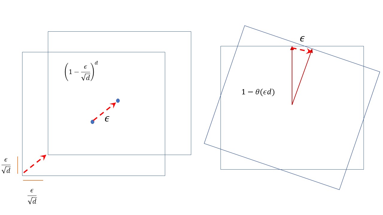
Figure 1: Shifting a cube in Euclidean norm or rotating can create very large TV distance.

The robust covariance and higher-moment estimation methods of  [15] can be used to robustly learn the columns of the unknown linear transformation each to within $\varepsilon$ error in Euclidean norm (after normalizing the covariance to be the identity). However, $\varepsilon$ error in each column means a TV distance error of up to $1-(1-O(\varepsilon))^{d}$, again growing with the dimension.

Our Result:

The main contribution of this paper is developing an algorithm for learning affine transformations that circumvents the inherent issues with the method of moments and manages to obtain, using polynomial time and samples, almost optimal recovery guarantees in total variation distance. Specifically, our main result is a polynomial-time algorithm to robustly estimate an unknown affine transformation of the hypercube to within TV distance $O(\varepsilon)$.

Theorem 1.1.

Given $Y=\{y_{\_}1,\ldots,y_{\_}n\}$, an $\varepsilon$-corrupted sample of points from an unknown parallelopiped $H=A[-1,1]^{d}+a$ in ${\mathbb R}^{d}$, there is a polynomial-time algorithm that outputs a parallelopiped $\widehat{H}=\widehat{A}[-1,1]^{d}+\widehat{a}$ s.t. $d_{\_}{TV}(\hat{H},H)=O(\varepsilon)$.

Our algorithm is based on a new approach to ICA, even without outliers, that does not rely on constant-order moments as in prior works. As we discuss next, a key contribution of our work is the development of a new certificate of correctness of the estimated linear transformation that does not rely on low order moments. Our algorithm relies on an iterative update step that makes progress whenever the current guess on the unknown affine transformation fails a check in the certificate.

1.1 Approach and techniques

Let us first assume the affine transformation consists of only a shift and a diagonal scaling. In this case, we start with a coarse approximation of the center and side lengths obtained by using the coordinate-wise median, and a scaling of the interval in each coordinate that contains the middle $(1/2)+\varepsilon$ fraction of samples. We then refine this iteratively using the fact that density of the cube is uniform along each coordinate, and, crucially, that the measure of the intersection of two axis-parallel bands is bounded by the product of their individual measures. If the latter condition is violated, then the intersection has a large fraction of corrupted samples, and we simply delete all the points in the intersection and continue. A simple and important idea here is that most of the corrupted points can be partitioned among the coordinate directions.

Now consider a general rotation, i.e., $A$ is orthonormal and $a=0$. This turns out to be substantially more challenging. The following bound on the TV distance serves as a starting point.

Lemma 1.2.

Let $H=[-1,1]^{d}$. Suppose $A,\widehat{A}$ are $d\times d$ matrices; $A$ is orthonormal and $\widehat{A}$ is a matrix with unit length rows. There is an absolute constant $C$ s.t.

$$d_{\_}{TV}(\widehat{A}H,AH)\leq C\sum_{\_}i\lVert\widehat{a}_{\_}i-a_{\_}i\rVert_{\_}2.$$

This lemma follows from Lemma 4.5, in which we prove the fraction of the volume of $\{x\in AH:x\cdot\widehat{a}_{\_}i>1\}$ is tightly bounded by $C\lVert\widehat{a_{\_}i}-a_{\_}i\rVert_{\_}2$. Crucially, the RHS terms are not squared. If they were, it would be the Frobenius norm and we can hope to robustly estimate to within low error. This norm however is not rotationally invariant, depends on the target basis (as it should!), and could be much larger.

To learn a rotation, we start with a coarse approximation, where each facet normal is approximated to within poly($\varepsilon$) error. Then, we consider one vector at a time (keeping the others fixed) and iteratively “improve" it. Our desired objective is to maximize the number of uncorrupted sample points inside the parallelopiped defined by the current vectors. But this is hard to estimate or improve locally. Instead, we focus on minimizing the number of points outside the band $|\widehat{a}_{\_}i^{\top}x|\leq 1$. We do this by proving that if the current distance $\|\widehat{a}_{\_}i-a_{\_}i\|_{\_}2=\delta$, then the mean of points in the difference in this direction i.e., $S=\{x:\widehat{a}_{\_}i^{\top}x\geq 1,|a_{\_}i^{T}x|\leq 1\}$ gives us an indication of which direction to move $\widehat{a}_{\_}i$ to make it closer to $a_{\_}i$. In other words, we can improve the objective of number of points outside the band by a local update. However, the presence of outliers complicates matters, as a small number of outliers could radically alter the location of the mean outside the band. To address this challenge, we prove that estimating the mean of this subset $S$ robustly in Euclidean norm suffices to preserve the gradient approximately! Alongside, to keep the influence of noise under control, we ensure that pairwise intersections of bands are all small. Roughly speaking, our algorithm is robust gradient descent with provable guarantees.

We combine the above procedures by alternating between them to robustly learn arbitrary affine transformations.

2 Preliminaries

2.1 Robust Estimation

Theorem 2.1 (Robust Mean Estimation for Bounded Covariance Distributions).

[11] There exists a polynomial time algorithm that takes input an $\varepsilon$-corruption sample of a collection $X$ of $n$ points in ${\mathbb R}^{d}$ where the mean of $X$ is $\mu$ and the covariance of $X$ is $\Sigma$ and outputs an estimate $\tilde{\mu}$ satisfying

$$\lVert\tilde{\mu}-\mu\rVert_{\_}2\leq O(\sqrt{\varepsilon})\lVert\Sigma\rVert_{\_}2^{1/2}.$$

Theorem 2.2 (Theorem 1.4 in [16], see also [17]).

There exists a polynomial time algorithm that given a corrupted sample $X$ of n points in ${\mathbb R}^{d}$ drawn from a rotated cube $AH$ where $A\in{\mathbb R}^{d\times d}$ is a orthogonal matrix with rows $a_{\_}1,\dots,a_{\_}d$, outputs component estimates $\hat{a}_{\_}1,\dots,\hat{a}_{\_}d\in{\mathbb R}^{d}$ with the following guarantee: the components estimates satisfy with high probability, there exists a permutation $\pi\in S_{\_}d$ such that for any $i\in[d]$,

$$\langle\hat{a}_{\_}i\cdot a_{\_}{\pi(i)}\rangle^{2}\geq 1-O(\sqrt{\varepsilon}).$$

2.2 Logconcave functions

The following lemmas are either from [18] or direct consequences.

Lemma 2.3.

Let $f:{\mathbb R}^{2}\rightarrow{\mathbb R}_{\_}+$ be an isotropic two-dimensional logconcave density with associated measure $\nu$. Let $u,v$ be unit vectors in ${\mathbb R}^{2}$ with $|u^{\top}v|\leq\frac{1}{2}$. Consider the bands $H_{\_}u=\{x:u^{\top}x\geq a_{\_}u\}$ and $H_{\_}v=\{x:v^{\top}x\geq a_{\_}v\}$ and assume that the marginal densities along $u$ and $v$, $f_{\_}u$ and $f_{\_}v$ satisfy $f_{\_}u(a_{\_}u),f_{\_}v(a_{\_}v)\geq 1/2$. Then, for a universal constant $C$,

$$\nu(H_{\_}u\cap H_{\_}v)\leq C\nu(H_{\_}u)\nu(H_{\_}v)$$

Lemma 2.4.

Let $f$ be a one-dimensional logconcave density with mean $0$ and variance $\sigma^{2}$. Let $\mu^{+}={\mathbb E}_{\_}f(y|y\geq 0)$. Then there exist universal constants $c_{\_}1,c_{\_}2$ s.t.

$$c_{\_}1\sigma\leq\mu^{+}\leq c_{\_}2\sigma.$$

Lemma 2.5.

For any one-dimensional logconcave density $f:{\mathbb R}\rightarrow{\mathbb R}_{\_}+$ with mean $\mu$, we have

$$\Pr(X\geq\mu)\geq\frac{1}{e}.$$

Lemma 2.6.

Let $f$ be a one-dimensional logconcave density with mean $\mu$. Then

$$f(\mu)\geq\frac{1}{8}\max f(x).$$

Lemma 2.7.

Suppose $M_{\_}n(f)$ are the moments of $f$, i.e.,

$$M_{\_}n(f)=\int_{\_}0^{\infty}t^{n}f(t)\;dt.$$

If $f$ is logconcave, then the sequence $M_{\_}n(f)/n!$ is logconcave.

2.3 Cubes

The following facts about cubes will be useful. While the precise constants in the bounds are not important for our analysis, the first two facts have been a subject of inquiry in asymptotic convex geometry.

Lemma 2.8.

[5] Let $B=[-1/2,1/2]^{d}$ be the $d$-dimensional cube with volume 1 and $a\in{\mathbb R}^{d}$ be an arbitrary unit vector. Then for all $t\leq 3/4$,

$$\mathrm{vol}(\{x\in B:|x\cdot a|>\frac{t}{2}\})\leq 1-t.$$

Lemma 2.9.

[4] Let $B=[-1/2,1/2]^{d}$ be the $d$-dimensional cube with volume 1 and $a\in{\mathbb R}^{d}$ be an arbitrary unit vector.. Then $(d-1)$-volume of any sections of $B$ defined by $a$ and $t$ is at most $\sqrt{2}$

$$\mathrm{vol}_{\_}{n-1}(\{x\in B:x\cdot a=t\})\leq\sqrt{2}.$$

The next fact follows from the above lemma and a calculation using the logconcavity of one-dimensional marginals of the hypercube.

Lemma 2.10.

Let $x\sim[-1,1]^{d}$ be a uniform random vector on $H=[-1,1]^{d}$ and $y=x\cdot a$ where $a$ is an arbitrary unit vector. Let $\mu_{\_}t={\mathbb E}_{\_}f(y|y\geq t)$. For $0\leq t\leq 1/2$, there exists universal constant $c$ s.t.

$$\mu^{t}\geq t+c.$$

3 Robustly learning a Shift and Diagonal Scaling

In this section, we give an algorithm for robustly learning arbitrary shifts and diagonal scalings of the uniform distribution on the solid hypercube $H=[-1,1]^{d}$. That is, $x\rightarrow Ax+b$ when $A$ is a diagonal matrix. Since the uniform distribution on $H$ is symmetric around $0$, we can WLOG assume that all the entries of $A$ are non-negative. This special case is equivalent to learning affine transformations that correspond to a shift (i.e., introducing a non-zero mean) and scaling (i.e., scales each of the coordinates of the hypercube by an unknown and potentially different positive scaling factor).

More precisely, we will prove:

Theorem 3.1.

Suppose $H$ is an unknown axis-aligned cube in ${\mathbb R}^{d}$, that is, $H=AH_{\_}0+b=\otimes_{\_}{i=1}^{d}[u_{\_}i,v_{\_}i]$ where $A\in{\mathbb R}^{d\times d}$ is a diagonal matrix, $b\in{\mathbb R}^{d}$ and $H_{\_}0=[-1,1]^{d}$ is the unit cube. There exists an algorithm that, for small enough constant $\varepsilon>0$, takes an $\varepsilon$-corruption $X=x^{(1)},x^{(2)},\ldots,x^{(n)}$ of size $n\geq n_{\_}0=\mathrm{poly}(d,1/\varepsilon)$ of an iid sample from the uniform distribution on $H$ and outputs $\widehat{H}=\widehat{A}H_{\_}0+\widehat{b}$ such that

$$d_{\_}{TV}(H,\widehat{H})\leq 4\varepsilon.$$

Remark 3.2.

While we will omit this refinement here, a more careful analysis of our algorithm produces a tighter bound of $d_{\_}{TV}(H,\widehat{H})\leq(2+\varepsilon)\varepsilon$.

We first describe our algorithm:

Algorithm 3.3.

1. Input: An $\varepsilon$-corruption $X$ of an iid sample of size $n$ chosen from $\otimes_{\_}{i=1}^{d}[u_{\_}i,v_{\_}i]$.

2. Robust Range Finding: For each $1\leq i\leq d$, arrange the input corrupted sample in increasing order of $y_{\_}i$. Let $[l_{\_}i,r_{\_}i]$ be the interval of the smallest length that includes the middle $1/2+\varepsilon$ fraction of the points (notice that such an interval is uniquely defined). Set $\hat{u}_{\_}i=2l_{\_}i$ and $\hat{v}_{\_}i=2r_{\_}i$. Notice that $\{x\in{\mathbb R}^{d}:v_{\_}i\leq x_{\_}i\leq u_{\_}i\}$ is an axis-aligned cube that contains the true cube and all the side lengths are at most twice the true cube.

3. One-Dimensional Density Check: For all $i\in[n],k\in[d]$, check if

   $$|S_{\_}{i,k}^{+}|:=\left|\left\{x:x^{(i)}\geq\left(1-\frac{k\varepsilon}{d}\right)\hat{u}_{\_}i+\frac{k\varepsilon}{d}\hat{v}_{\_}i\right\}\right|\geq\frac{k\varepsilon}{2d}n$$ (1)

   $$|S_{\_}{i,k}^{-}|:=\left|\left\{x:x^{(i)}\leq\frac{k\varepsilon}{d}\hat{u}_{\_}i+\left(1-\frac{k\varepsilon}{d}\right)\hat{v}_{\_}i\right\}\right|\geq\frac{k\varepsilon}{2d}n$$ (2)

4. Update: If (1) is false for some $i$ and $k$, update $\hat{u}_{\_}i=\hat{u}_{\_}i-\frac{k\varepsilon}{d}(\hat{u}_{\_}i-\hat{v}_{\_}i)$ and go back to Step 3. If (2) is false for some $i$ and $k$, set $\hat{v}_{\_}i=\hat{v}_{\_}i+\frac{k\varepsilon}{d}(\hat{u}_{\_}i-\hat{v}_{\_}i)$ and iterate (go back to Step 3).

5. Two-Dimensional Density Check: For all $i,j\in[n],k_{\_}1,k_{\_}2\in[d]$, check if

   $$|S_{\_}{i,k_{\_}1}^{+}\cap S_{\_}{j,k_{\_}2}^{+}|,|S_{\_}{i,k_{\_}1}^{+}\cap S_{\_}{j,k_{\_}2}^{-}|,|S_{\_}{i,k_{\_}1}^{-}\cap S_{\_}{j,k_{\_}2}^{-}|\leq\frac{10k_{\_}1k_{\_}2\varepsilon^{2}}{d^{2}}n$$ (3)

6. Update: If (3) is false for some $i,j$ and $k_{\_}1,k_{\_}2$, remove all points in the violating intersection from the sample set and go back to Step 3.

7. Return: Output the cube $\otimes_{\_}{i=1}^{d}[\hat{u}_{\_}i,\hat{v}_{\_}i]$.

Notice that in this case, our goal is effectively to determine the intervals $[u_{\_}i,v_{\_}i]$ for each $1\leq i\leq d$ that describe the $i$-th dimension of the shifted and scaled hypercube $H$. The key idea of the algorithm is a certificate that checks a set of efficiently verifiable conditions on the corrupted sample with the guarantee that 1) the true parameters satisfy the checks, and 2) any set of parameters that satisfy the checks yield a hypercube $\hat{H}$ that is $O(\varepsilon)$ different in symmetric volume difference (that gives us a total variation bound) from the true hypercube $H$.

Our certificate itself is simple and natural and corresponds to checking that 1) for each of the coordinates $1\leq i\leq d$, the discretized density (i.e., fraction of points lying in discrete intervals of size $\sim\varepsilon/d$ in the purported range estimated from the corrupted sample matches the expected density of the uniform distribution on $AH+b$, and 2) for each pair of coordinates, the fraction of points in the intersection of intervals of length $\sim\varepsilon/d$ along all possible pairs of directions match the expected density. Notice that all such statistics in an uncorrupted sample match those of the population with high probability so long as the the sample is of size $\mathrm{poly}(d/\varepsilon)$.

To analyze the above algorithm, we will prove that any set of parameters that satisfy the checks in our certificate (1),(2),(3) in Algorithm 3.3 must yield a good estimate of true parameters. Specifically, Lemma 3.5 shows that the volume of $\widehat{H}$ that is not contained in $H$ is small. Lemma 3.7 shows that the volume of $H$ that is not covered by $\widehat{H}$ is small. Together, these two lemmas imply that our estimated distribution is $O(\varepsilon$) close in total variation to the true hypercube. Our proof relies on an elementary combinatorial claim about set systems that we state next. We defer the proof to Section 6.

Lemma 3.4.

Let $S_{\_}1,\dots,S_{\_}d\subseteq[n]$ be arbitrary subsets. Let $\mathrm{frac}(S):=|S|/n$ be normalized size of $S$. Suppose that

$$\mathrm{frac}\left(\bigcup S_{\_}i\right)=\varepsilon$$ (4)

for some $\varepsilon<1$ and for all $i,j$,

$$\mathrm{frac}(S_{\_}i\cap S_{\_}j)\leq\alpha\mathrm{frac}(S_{\_}i)\mathrm{frac}(S_{\_}j),$$ (5)

for some $\alpha>0$ s.t. $\alpha\varepsilon<1$. Then,

$$\sum_{\_}{i\in[d]}\mathrm{frac}(S_{\_}i)\leq\frac{\varepsilon}{1-\alpha\varepsilon}.$$ (6)

Lemma 3.5.

Let $X=\{x^{(1)},x^{(2)},\ldots,x^{(n)}\}$ be an $\varepsilon$-corruption of an iid sample from the uniform distribution on $H=\otimes_{\_}{i=1}^{d}[u_{\_}i,v_{\_}i]$. Let $\widehat{H}=\otimes_{\_}{i=1}^{d}[\hat{u}_{\_}i,\hat{v}_{\_}i]$ be any axis-aligned hypercube satisfying (1),(2),(3). Then, with probability at least $1-1/d$ over the draw of the original uncorrupted sample,

$$\frac{\mathrm{vol}(\widehat{H}\setminus H)}{\mathrm{vol}(\widehat{H})}\leq 4\varepsilon.$$

Here, $\mathrm{vol}$ denotes the usual Lebesgue volume of sets in ${\mathbb R}^{d}$.

Proof.

For only the sake of analysis, we set $\hat{u}_{\_}i-\hat{v}_{\_}i=1$. In this normalization, $\mathrm{vol}(\widehat{H})=1$. For each $i$, discretize the interval $[\hat{u}_{\_}i,\hat{v}_{\_}i]$ to a grid with intervals of size $\varepsilon(\hat{u}_{\_}i-\hat{v}_{\_}i)/d=\varepsilon/d$. We further assume that the vertices of the unknown $H$ are rounded to points in this grid. This assumption amounts to a change in the volume of $H$ by at most $\varepsilon\mathrm{vol}(\hat{H})$. We will then show that the density of points in the difference $\widehat{H}\setminus H$, i.e., $\{x:x\in\widehat{H},x\notin H\}$ is

$$\frac{|\{x\in X:x\in\widehat{H}\setminus H\}|}{\mathrm{vol}(\widehat{H}\setminus H)}\geq\frac{1}{4}n.$$ (7)

From the inequality above, it follows that $\mathrm{vol}(\widehat{H}\setminus H)\leq\frac{4}{n}|\{x:x\in\widehat{H}\setminus H\}|\leq 4\varepsilon$ since $|\{x:x\in\widehat{H}\setminus H\}|\leq\varepsilon n$. So it suffices to prove (7).

For all $i\in[d]$, suppose $u_{\_}i-\hat{u}_{\_}i=c_{\_}i\varepsilon/d,\hat{v}_{\_}i-v_{\_}i=c_{\_}i^{\prime}\varepsilon/d$. Let $S_{\_}i=\{x\in X:\hat{u}_{\_}i\leq x_{\_}i\leq u_{\_}i,v_{\_}i\leq x_{\_}i\leq\hat{v}_{\_}i\}$. By (1) and (2), we have $|S_{\_}i|\geq(c_{\_}i+c_{\_}i^{\prime})\frac{\varepsilon}{2d}n$. By (3), we have for any $i\neq j$,

$$|S_{\_}i\cap S_{\_}j|\leq 10(c_{\_}i+c_{\_}i^{\prime})\frac{\varepsilon^{2}}{d^{2}}n\leq 40|S_{\_}i||S_{\_}j|n.$$

Then by Lemma 3.4 with $\alpha=40$,

$$\frac{|\bigcup S_{\_}i|}{n-40|\bigcup S_{\_}i|} \geq\sum_{\_}{i\in[d]}\frac{|S_{\_}i|}{n},$$

$$\frac{|\{x:x\in\widehat{H}\setminus H\}|}{n-40|\{x:x\in\widehat{H}\setminus H\}|} \geq\frac{\varepsilon}{2d}\sum_{\_}{i=1}^{d}(c_{\_}i+c_{\_}i^{\prime}).$$

By the upper bound on the total number $|\{x:x\in\widehat{H}\setminus H\}|\leq\varepsilon n\leq n/80$, the denominator is at least $n/2$. Then

$$|\{x:x\in\widehat{H}\setminus H\}|\geq\frac{\varepsilon}{4d}n\sum_{\_}{i=1}^{d}(c_{\_}i+c_{\_}i^{\prime}).$$

Thus we get (7) by $\mathrm{vol}(\widehat{H}\setminus H)\leq\frac{\varepsilon}{d}\sum_{\_}{i=1}^{d}(c_{\_}i+c_{\_}i^{\prime})$. ∎

Next we show that Step 6 removes at most $\varepsilon n$ true points in total.

Lemma 3.6.

With high probability, at least half of points removed in Step 6 are outliers.

Proof.

Suppose we remove points from an intersection $S_{\_}{i,k_{\_}1}^{+}\cap S_{\_}{j,k_{\_}2}^{+}$, i.e.,

$$|S_{\_}{i,k_{\_}1}^{+}\cap S_{\_}{j,k_{\_}2}^{+}|>\frac{10k_{\_}1k_{\_}2\varepsilon^{2}}{d^{2}}n.$$ (8)

If the violating intersection is outside the true cube, all the points are outliers. Otherwise, we can compute the volume by definition of $S_{\_}{i,k}^{+}$

$$\mathrm{vol}(S_{\_}{i,k_{\_}1}^{+}\cap S_{\_}{j,k_{\_}2}^{+})=\frac{k_{\_}1k_{\_}2\varepsilon^{2}}{d^{2}}(\hat{u}_{\_}i-\hat{v}_{\_}i)(\hat{u}_{\_}j-\hat{v}_{\_}j)\leq\frac{4k_{\_}1k_{\_}2\varepsilon^{2}}{d^{2}}$$

where the last equality follows from $\hat{u}_{\_}i-\hat{v}_{\_}i$ is at most twice of the true side length. Then with high probability, the number of original uncorrupted sample in the region $S_{\_}{i,k_{\_}1}^{+}\cap S_{\_}{j,k_{\_}2}^{+}$ of volume $4k_{\_}1k_{\_}2\varepsilon^{2}/d^{2}$ is at most $5k_{\_}1k_{\_}2\varepsilon^{2}n/d^{2}$. Thus, comparing with (8), we can see that at least half of the point removed by the algorithm are outliers. ∎

Lemma 3.7.

Let $X=\{x^{(1)},x^{(2)},\ldots,x^{(n)}\}$ be an $\varepsilon$-corruption of an iid sample from the uniform distribution on $H=\otimes_{\_}{i=1}^{d}[u_{\_}i,v_{\_}i]$. Let $\widehat{H}=\otimes_{\_}{i=1}^{d}[\hat{u}_{\_}i,\hat{v}_{\_}i]$ be an axis-aligned hypercube satisfying (1),(2),(3). Then, with probability at least $1-1/d$ over the draw of the original uncorrupted sample,

$$\frac{\mathrm{vol}(H\setminus\widehat{H})}{\mathrm{vol}(H)}\leq 4\varepsilon.$$

Proof.

For only the sake of analysis, we set $\hat{u}_{\_}i-\hat{v}_{\_}i=1$ and $\mathrm{vol}(\widehat{H})=1$. For $i\in[d]$ s.t. $\hat{u}_{\_}i<u_{\_}i$ or $v_{\_}i<\hat{v}_{\_}i$, we define $S_{\_}i=\{x:\hat{u}_{\_}i<x_{\_}i\leq u_{\_}i,v_{\_}i\leq x_{\_}i<\hat{v}_{\_}i\}$ and $c_{\_}i=u_{\_}i-\hat{u}_{\_}i,c_{\_}i^{\prime}=\hat{v}_{\_}i-v_{\_}i$. Then

$$H\setminus\widehat{H}=\bigcup_{\_}{\{i:\hat{u}_{\_}i<u_{\_}i,\text{ or }v_{\_}i<\hat{v}_{\_}i\}}S_{\_}i.$$

Since $S_{\_}i$ are removed by the algorithm, by (1) and (2), $|S_{\_}i|<\frac{1}{2}(c_{\_}i+c_{\_}i^{\prime})n$. Since $S_{\_}i$ is in the true cube, the original uncorrupted sample in $S_{\_}i$ is at least $(c_{\_}i+c_{\_}i^{\prime})n$ with high probability. So there are at least half of the original uncorrupted sample in $S_{\_}i$ are removed by either the adversary or by the algorithm. Suppose $\eta_{\_}in$ is the number of original uncorrupted sample removed in $S_{\_}i$. Then $\eta_{\_}i\geq\frac{1}{2}(c_{\_}i+c_{\_}i^{\prime})$. By Lemma 3.6, the total number of points deleted by the algorithm is at most $\varepsilon n$. Hence the number of deleted points in $\bigcup S_{\_}i$ is at most $2\varepsilon n$. The deletion in the intersection of $S_{\_}i$ and $S_{\_}j$ is naturally upper bounded by the number of original uncorrupted sample. So we can apply Lemma 3.4 with $\alpha=4$ to the deletion in $S_{\_}i$ and get

$$\frac{2\varepsilon}{1-8\varepsilon}\geq\sum_{\_}{\{i:\hat{u}_{\_}i<u_{\_}i,\text{ or }v_{\_}i<\hat{v}_{\_}i\}}\eta_{\_}i.$$

If $\varepsilon\leq 1/16$, the left hand side is at most $4\varepsilon$. Thus

$$\mathrm{vol}(H\setminus\widehat{H})=\mathrm{vol}\left(\bigcup S_{\_}i\right) \leq\sum\mathrm{vol}(S_{\_}i)$$

$$\leq\frac{1}{2}\sum(c_{\_}i+c_{\_}i^{\prime})$$

$$\leq\sum\eta_{\_}i$$

$$\leq 4\varepsilon.$$

∎

Now, with Lemmas 3.5 and 3.7, we can prove our main result of the shift and scaling case.

Proof of Theorem 3.1.

If the algorithm outputs a cube $\widehat{H}$ satisfies (1),(2),(3), then by Lemma 3.5 and Lemma 3.7,

$$d_{\_}{TV}(H,\widehat{H})=1-\frac{\mathrm{vol}(H\cap\widehat{H})}{\max\{\mathrm{vol}(H),\mathrm{vol}(\widehat{H})\}}=\max\left\{\frac{\mathrm{vol}(H\setminus\widehat{H})}{\mathrm{vol}(H)},\frac{\mathrm{vol}(\widehat{H}\setminus H)}{\mathrm{vol}(\widehat{H})}\right\}=4\varepsilon.$$

Otherwise, the algorithm improves one of $\hat{u}_{\_}i$ or $\hat{v}_{\_}i$ by at least $\varepsilon/d$. Thus, within at most $O(d^{2}/\varepsilon)$ iterations, the algorithm terminates. If the algorithm terminates when it deletes $2\varepsilon n$ points, by Lemma 3.6, we remove all noisy points. ∎

4 Rotation

In this section, we give a robust algorithm to learn rotations of the uniform distribution of the standard hypercube. Specifically, we will show:

Theorem 4.1.

Suppose $H=[-1,1]^{d}$ is the standard cube in ${\mathbb R}^{d}$ and $A\in{\mathbb R}^{d\times d}$ be an unknown rotation matrix. There exists an algorithm that given an $\varepsilon$-corruption $X=\{x^{(1)},\dots,x^{(n)}\}$ of size $n\geq n_{\_}0=\mathrm{poly}(d,1/\varepsilon)$ of an iid sample from the uniform distribution on $AH$, runs in poly($n$) time and outputs $\widehat{A}$ such that

$$d_{\_}{TV}(AH,\widehat{A}H)=O(\varepsilon).$$

We first describe the algorithm:

Algorithm 4.2.

Input: $\varepsilon$-corrupted sample $X=\{x^{(1)},x^{(2)},\ldots,x^{(n)}\}$.

Output: $\widehat{A}$ with unit length rows $\hat{a}_{\_}{(1)},\dots,\hat{a}_{\_}{(d)}$.

1. Warm Start: Run the robust moment estimation algorithm in Theorem 2.2 and get an estimate of $A$ with rows $a_{\_}{(1)}^{*},\dots,a_{\_}{(d)}^{*}$, so that for each $i$, $\lVert\hat{a}_{\_}{(i)}-a_{\_}{(i)}^{*}\rVert_{\_}2=O(\sqrt{\varepsilon})$. Initialize $a_{\_}{(i)}^{0}=\hat{a}_{\_}{(i)}$ for each $i$.

2. For any vector $a\in{\mathbb R}^{d}$, let $S(a)=\{x:x\cdot a>1\}\cup\{-x:x\cdot a<-1\}$. For $t=1,2,\ldots,2^{12}d\log d$, do:

   1. Two-Dimensional Density Check: For all $j<i$, check if

      $$\frac{1}{n}|S(a_{\_}{(i)}^{t})\cap S(\hat{a}_{\_}{(j)})|>\frac{2c_{\_}1}{n^{2}}|S(a_{\_}{(i)}^{t})||S(\hat{a}_{\_}{(j)})|$$

      If false, remove all points in the intersection $S(a_{\_}{(i)}^{t})\cap S(\hat{a}_{\_}{(j)})$.

   2. Robust GD: Robustly estimate the mean $\tilde{\mu}$ by applying algorithm in Theorem 2.1 to the subset $S(a_{\_}{(i)}^{t})$. Set

      $$\beta =\frac{c_{\_}2|S(a_{\_}{(i)}^{t})|}{\lVert\tilde{\mu}\rVert^{2}n},$$

      $$a_{\_}{(i)}^{t+1} =\frac{a_{\_}{(i)}^{t}-\beta\tilde{\mu}}{\lVert a_{\_}{(i)}^{t}-\beta\tilde{\mu}\rVert}$$

      $$s^{t+1} =\left|\{x:|x\cdot a_{\_}{(i)}^{t+1}|>1\}\right|$$

      Add back points that are removed in Step (a), i.e., recover the sample set to the origin one $X$.

   Let $\hat{a}_{\_}{(i)}=a_{\_}{(i)}^{t}$ where $t$ minimizes $s^{t}$.

3. Output the matrix $\widehat{A}$ with rows $\hat{a}_{\_}{(1)},\dots,\hat{a}_{\_}{(d)}$.

4.1 Outline of analysis

For the purpose of analysis, we assume that the true rotation matrix is the identity matrix in the rest of Section 4. We will analyze Algorithm 4.2 by the following propositions. First we show that we can separately learn the rows of the rotation matrix. Let $S(a)=\{x:x\cdot a>1\}\cup\{-x:x\cdot a<-1\}$. For a set of unit vectors $\hat{a}_{\_}{(1)},\dots,\hat{a}_{\_}{(d)}$ and a corrupted sample $X$, after we remove samples in all the intersections such that

$$\frac{1}{n}|S(\hat{a}_{\_}{(i)})\cap S(\hat{a}_{\_}{(j)})|>\frac{2c_{\_}1}{n^{2}}|S(\hat{a}_{\_}{(i)})||S(\hat{a}_{\_}{(j)})|$$

as in Step 2(a) of Algorithm 4.2, we can define $\varepsilon_{\_}i$ as the fraction of outliers in $S(\hat{a}_{\_}{(i)})$ and $\eta_{\_}i$ as the fraction of original uncorrupted sample in $S(\hat{a}_{\_}{(i)})$ that are removed by the adversary or by the algorithm. That is, $\varepsilon_{\_}i$ and $\eta_{\_}i$ are exactly the fraction of corrupted samples when we robustly estimate $\tilde{\mu}$. In the following Proposition, we show that the sum of $\varepsilon_{\_}i$ and $\eta_{\_}i$ is small, which implies we do not increase the fraction of outliers by separately learning $a_{\_}{(1)},\dots,a_{\_}{(d)}$.

Proposition 4.3.

Let $X_{\_}i$ be the subset of corrupted sample $X$ after removing samples in Step 2(a) of Algorithm 4.2 and $S(\hat{a}_{\_}{(i)})=\{x:x\cdot\hat{a}_{\_}{(i)}>1,x\in X_{\_}i\}\cup\{-x:x\cdot\hat{a}_{\_}{(i)}<-1,x\in X_{\_}i\}$. Let $\varepsilon_{\_}i$ be the fraction of outliers in $S(\hat{a}_{\_}{(i)})$, and $\eta_{\_}i$ be the fraction of original uncorrupted sample in $S(\hat{a}_{\_}{(i)})$ that are removed by the adversary or the algorithm. Suppose for all $i$, $\hat{a}_{\_}{(i)}\cdot e_{\_}i\geq 0.99$ and for all $i,j$,

$$\frac{1}{n}|S(\hat{a}_{\_}{(i)})\cap S(\hat{a}_{\_}{(j)})|\leq\frac{2c_{\_}1}{n^{2}}|S(\hat{a}_{\_}{(i)})||S(\hat{a}_{\_}{(j)})|.$$

Then,

$$\sum_{\_}{i\in[d]}(\varepsilon_{\_}i+\eta_{\_}i)\leq 2\varepsilon.$$

The proof of Proposition 4.3 is deferred to Section 4.3.

Next, we give a robust algorithm that updates a single rotation vector $\hat{a}_{\_}{(i)}$ of the cube with a small constant fraction of corruption in $\{x:|x\cdot\hat{a}_{\_}{(i)}|>1\}$. We show that by repeatedly applying this algorithm on $\hat{a}_{\_}{(i)}$ at most $O(d\log d)$ times, we can learn the rotation vector $e_{\_}i$ with error $O(\varepsilon_{\_}i+\eta_{\_}i)$.

Proposition 4.4.

Suppose $H=[-1,1]^{d}$ is the true hypercube. There exists a robust algorithm that given $\varepsilon$-corrupted samples from $H$ and a unit vector $a_{\_}{(i)}^{0}$ such that $\lVert a_{\_}{(i)}^{0}-e_{\_}i\rVert_{\_}2\leq 0.1$, outputs

$$\lVert\hat{a}_{\_}{(i)}-e_{\_}i\rVert_{\_}2\leq 2^{14}(\varepsilon_{\_}i+\eta_{\_}i)$$

after at most $2^{12}d\log d$ iterations, where $\varepsilon_{\_}i+\eta_{\_}i$ is the fraction of corruption in $\{x:x\cdot\hat{a}_{\_}{(i)}>1\}$.

The proof of Proposition 4.4 is deferred to Section 4.4. With the two propositions above, we complete the proof of Theorem 4.1 in Section 4.5.

4.2 Properties of Cubes

In this section, we prove a few basic properties of uniform samples from $H=[-1,1]^{d}$, in particular, of the subset of samples $\{x\in H:x\cdot a>1\}$ for a unit vector $a$. We will later use them in our analysis of Algorithm 4.2.

The following lemma is crucial for our analysis since it connects the 2-norm error of $\hat{a}_{\_}{(i)}$ and the volume of $\widehat{A}H\setminus AH$. Hence it implies Lemma 1.2.

Lemma 4.5.

Let $Y$ be a uniform sample from $H$ of size $n$. Suppose $a$ is a unit vector such that $\lVert a-e_{\_}i\rVert=\delta$. Then with high probability the number of samples in $S(a)\cap Y$ is

$$\frac{\delta}{5}n\leq|S(a)\cap Y|:=\left|\left\{x\in Y:|x\cdot a|>1\right\}\right|\leq\frac{(1+\delta)\delta}{4}n.$$

Proof.

Let $\bar{a}$ be the $d-1$-vector that excludes $i$-th coordinate of $a$. Since $\lVert a-e_{\_}i\rVert=\delta$, we have that $a_{\_}{i}=a\cdot e_{\_}i=1-\delta^{2}/2$ and $\lVert\bar{a}\rVert=\delta+O(\delta^{2})$. Let $S^{+}(a):=\{x:x\cdot a>1\}$. By symmetry of the cube, $2\mathrm{vol}(S^{+}(a))=\mathrm{vol}(S(a))$. So it suffices to compute the number of original uncorrupted sample in $S^{+}(a)$ and double it. We can compute the volume of $S^{+}(a)$ by integrating the length of $x_{\_}i$ over $\bar{x}$ where $\bar{x}$ is the vector $x$ without entry $x_{\_}i$. The upper bound on $\bar{x}$ is 1 and the lower bound is $x\cdot a=1$, i.e., $x_{\_}i=\frac{1-\bar{x}\cdot\bar{a}}{a_{\_}i}$. So we have

$$\mathrm{vol}(S^{+}(a))=\int_{\_}{\bar{x}\in[-1,1]^{d-1}}\max\left\{0,1-\frac{1-\bar{x}\cdot\bar{a}}{a_{\_}i}\right\}\;d\bar{x}$$

Let $y=\bar{x}\cdot\bar{a}$. Suppose $p(y)$ is the density of $y$. Let $1-\frac{1-\bar{x}\cdot\bar{a}}{a_{\_}i}\geq 0$. We have $y\geq\delta^{2}/2$. Thus, we can write the integral above as

$$\mathrm{vol}(S^{+}(a))=2^{d-1}\left(\Pr\left(y\geq\frac{\delta^{2}}{2}\right)\left(1-\frac{1}{a_{\_}i}\right)+\frac{1}{a_{\_}i}\int_{\_}{y\geq\frac{\delta^{2}}{2}}y\cdot p(y)\;dy\right).$$ (9)

Since $\bar{x}$ is a uniform random variable on $[-1,1]^{d-1}$, we have $y$ is a scaled 1d-projection of the standard $(d-1)$-cube onto an arbitrary direction with zero mean and variance $\lVert\bar{a}\rVert^{2}/3=\delta^{2}/3$. Since $y$ is logconcave and symmetric, we can bound the probability $1/2-\delta\leq\Pr\left(y\geq\frac{\delta^{2}}{2}\right)\leq 1/2$. We define $\mu_{\_}y:={\mathbb E}(y\mid y\geq\delta^{2}/2)=\int_{\_}{y\geq\frac{\delta^{2}}{2}}y\cdot p(y)\;dy$ as the truncated mean of $y$. Then

$$\mathrm{vol}(S^{+}(a))=2^{d-1}\Pr\left(y\geq\frac{\delta^{2}}{2}\right)\left(1-\frac{1}{a_{\_}i}+\frac{\mu_{\_}y}{a_{\_}i}\right)$$ (10)

By Lemma 2.4, $\mu_{\_}y$ is upper and lower bounded by $\Theta(\delta)$. The upper bound is achieved when $\bar{a}$ is in the direction of true coordinates, which is $(1+\delta)\delta/2$. Let $y^{+}$ be the truncated density of $y$ on ${\mathbb R}^{+}$. Then raw moments of $y^{+}$ are $M_{\_}0(y^{+})=1,M_{\_}1(y^{+})\leq\mu_{\_}y,M_{\_}2(y^{+})=\delta^{2}/3$. By Lemma 2.7, $M_{\_}1^{2}\geq M_{\_}0\frac{M_{\_}2}{2}$. Then $\mu_{\_}y\geq M_{\_}1\geq\frac{1}{\sqrt{6}}\delta\geq\frac{2}{5}\delta$. Plugging the bounds of $\Pr\left(y\geq\frac{\delta^{2}}{2}\right)$ and $\mu_{\_}y$ into (10), we get

$$\frac{2\delta}{5}-\frac{\delta^{2}}{2} \leq 1-\frac{1}{a_{\_}i}+\frac{\mu_{\_}y}{a_{\_}i}=\frac{\mu_{\_}y-\delta^{2}/2}{1-\delta^{2}/2}\leq\frac{\delta+\delta^{2}}{2}$$

$$\frac{2^{d-1}}{5}\delta n \leq\mathrm{vol}(S^{+}(a))\leq 2^{d-3}(1+\delta)\delta n.$$

Since the volume of the standard cube $H$ is $2^{d}$, the probability a uniformly random sample is in $S^{+}(a)$ is at least $2^{d-1}\delta/(5\cdot 2^{d})=\delta/10$ and at most $2^{d-3}(1+\delta)\delta/2^{d}=(1+\delta)\delta/8$. Thus the fraction of samples in $S(a)$ is at least $\delta/5$ and at most $(1+\delta)\delta/4$. ∎

Lemma 4.6.

Suppose $\lVert a-e_{\_}i\rVert=\delta$. Let $\mu$ be the mean of the subset of the cube: $\{x\in[-1,1]^{d}:a\cdot x>1\}$. Then $\mu\cdot e_{\_}i\leq 1-\delta/32$.

Proof.

Let $S^{+}(a)=\{x\in[-1,1]^{d}:x\cdot a>1\}$ and $S^{\prime}=\{x\in[-1,1]^{d}:x\cdot a>1,x_{\_}i=x\cdot e_{\_}i>1-c\delta\}$ for a fixed constant $c<1$. Then by the trivial upper bound: $x_{\_}i\leq 1$ for any $x$ in the cube,

$$\mu\cdot e_{\_}i\leq\frac{\mathrm{vol}(S^{\prime})+(1-c\delta)(\mathrm{vol}(S^{+}(a))-\mathrm{vol}(S^{\prime}))}{\mathrm{vol}(S^{+}(a))}=1-c\delta\left(1-\frac{\mathrm{vol}(S^{\prime})}{\mathrm{vol}(S^{+}(a))}\right).$$

We can compute the volume of $S^{\prime}$ by integral over $x_{\_}i$.

$$\frac{\mathrm{vol}(S^{\prime})}{\mathrm{vol}(H)} =\frac{1}{2}\int_{\_}{1-c\delta}^{1}\Pr(x\cdot a>1\mid x_{\_}i)\;dx_{\_}i$$

$$=\frac{1}{2}\int_{\_}{1-c\delta}^{1}\Pr(\bar{x}\cdot\bar{a}\geq 1-x_{\_}i\cdot a_{\_}i)\;dx_{\_}i$$

Let $y=\bar{x}\cdot\bar{a}/\lVert\bar{a}\rVert$. Since $x_{\_}1$ and $\bar{x}$ are independent, $\bar{x}$ is uniformly random over the $d-1$ standard cube and $y$ is the projection of $\bar{x}$ onto an arbitrary unit vector. Let $t=(1-x_{\_}i)/\delta$ and hence $x_{\_}i=1-t\delta$. Then $dx_{\_}i=-\delta\;dt$. By substitution,

$$\frac{\mathrm{vol}(S^{\prime})}{\mathrm{vol}(H)}=\frac{1}{2}\int_{\_}{t=0}^{c}\Pr\left(y\geq\frac{1-x_{\_}i\cdot a_{\_}i}{\lVert\bar{a}\rVert}\right)\delta\;dt\leq\frac{1}{2}\int_{\_}{t=0}^{c}\Pr(y\geq t)\delta\;dt$$

By Lemma 2.8, $\Pr(y\geq t)\leq 1/2(1-t)$ for any $t\leq 3/4$. Take $c=1/2$. Then we get

$$\frac{\mathrm{vol}(S^{\prime})}{\mathrm{vol}(H)}\leq\frac{1}{2}\int_{\_}{t=0}^{c}\frac{1}{2}(1-t)\delta\;dt=\frac{1}{4}(c-c^{2}/2)\delta=\frac{3}{32}\delta.$$

By Lemma 4.5, $\frac{\mathrm{vol}(S^{+}(a))}{\mathrm{vol}(H)}\geq\delta/10$. Thus

$$\mu\cdot e_{\_}i=1-c\delta\left(1-\frac{\mathrm{vol}(S^{\prime})}{\mathrm{vol}(S^{+}(a))}\right)\leq 1-\delta/32.$$

∎

Lemma 4.7.

Let $H$ be the standard hypercube $[-1,1]^{d}$. Suppose $\lVert a-e_{\_}i\rVert=\delta$. Then the variance of uniform distribution on $H\cap\{x:x\cdot a>1\}$ in the direction $e_{\_}i$ is at most $c\delta^{2}$.

Proof.

Suppose $p(x_{\_}i)$ is the density function of $x_{\_}i$ on $\{x:x\cdot a>1\}$ and $\bar{x},\bar{a}$ are vectors constructed from $x,a$ by excluding $i$-th coordinate. Then

$$p(x_{\_}i)\propto\mathrm{vol}_{\_}{d-1}(\{x:x\cdot a>1,x_{\_}i\text{ is fixed}\})\propto\Pr_{\_}{\bar{x}}(\bar{x}\cdot\bar{a}>1-a_{\_}ix_{\_}i).$$

Let $y=\bar{x}\cdot\bar{a}$. Then $y$ is logconcave and symmetric with mean 0 and variance $\delta^{2}/3$. So in the range $x_{\_}i\in[-1,1]$, $p(x_{\_}i)$ is increasing. Then

$$\max p(x_{\_}i)=p(1)\propto\Pr(y>\delta^{2}/2)\geq\frac{1}{2}-\delta.$$

and

$$p(1-\delta)\propto\Pr(y>1-a_{\_}i(1-\delta))\leq\Pr(y>\delta)\leq\frac{3-2\sqrt{2}}{4}.$$

If $\delta<0.1$, then $p(1-\delta)<\frac{1}{8}\max p(x_{\_}i)$. By Lemma 2.6, $p(\mu)\geq\frac{1}{8}\max p(x_{\_}i)$. By the monotonicity of $p(x_{\_}i)$, we have $\mu\geq 1-\delta$. Then by Lemma 2.4, the variance of $x_{\_}i$ on the whole subset is upper-bounded by the variance of one side of the mean. ∎

4.3 Rotation matrix can be learned coordinate by coordinate

In this section, we prove Proposition 4.3 via Lemmas 4.8 and 4.9. Recall that $S(\hat{a}_{\_}{(i)})=\{x:x\cdot\hat{a}_{\_}{(i)}>1\}\cup\{-x:x\cdot\hat{a}_{\_}{(i)}<-1\}$ and $\varepsilon_{\_}i$ is the fraction of outliers in $S(\hat{a}_{\_}{(i)})$, $\eta_{\_}i$ is the fraction of original uncorrupted sample in $S(\hat{a}_{\_}{(i)})$ that are removed.

Lemma 4.8.

Let $X_{\_}i$ be the subset of corrupted sample $X$ after removing samples in Step 2(a) of Algorithm 4.2 and $S(\hat{a}_{\_}{(i)})=\{x:x\cdot\hat{a}_{\_}{(i)}>1,x\in X_{\_}i\}\cup\{-x:x\cdot\hat{a}_{\_}{(i)}<-1,x\in X_{\_}i\}$. Let $\varepsilon_{\_}i$ be the fraction of outliers in $S(\hat{a}_{\_}{(i)})$. Suppose for all $i$, $\hat{a}_{\_}{(i)}\cdot e_{\_}i\geq 0.99$ and for all $i,j$,

$$\frac{1}{n}|S(\hat{a}_{\_}{(i)})\cap S(\hat{a}_{\_}{(j)})|\leq\frac{2c_{\_}1}{n^{2}}|S(\hat{a}_{\_}{(i)})||S(\hat{a}_{\_}{(j)})|.$$

Then $\sum_{\_}{i\in[d]}\varepsilon_{\_}i\leq 2\varepsilon$.

Proof.

Let $S_{\_}N(\hat{a}_{\_}{(i)})$ be the set of outliers that in the halfspace $\{x:x\cdot\hat{a}_{\_}{(i)}>1\}$. We know the fraction of all outliers is at most $\varepsilon$. So we have $\mathrm{frac}\left(\bigcup S_{\_}N(\hat{a}_{\_}{(i)})\right)\leq\varepsilon$. We may assume that $\varepsilon_{\_}i\geq c_{\_}3\mathrm{frac}(S(\hat{a}_{\_}{(i)}))$. Otherwise, we can reduce $\mathrm{frac}(S(\hat{a}_{\_}{(i)}))$ by running the update algorithm in Section 4.4 (Corollary 4.13). Then

$$\mathrm{frac}(S_{\_}N(\hat{a}_{\_}{(i)})\cap S_{\_}N(\hat{a}_{\_}{(j)}))\leq\mathrm{frac}(S(\hat{a}_{\_}{(i)})\cap S(\hat{a}_{\_}{(j)}))\leq 2c_{\_}1\mathrm{frac}(S(\hat{a}_{\_}{(i)}))\mathrm{frac}(S(\hat{a}_{\_}{(j)}))\leq\frac{2c_{\_}1}{c_{\_}3^{2}}\varepsilon_{\_}i\varepsilon_{\_}j.$$

Set $\alpha=\frac{2c_{\_}1}{c_{\_}3^{2}}$, we get

$$\mathrm{frac}(S_{\_}N(\hat{a}_{\_}{(i)})\cap S_{\_}N(\hat{a}_{\_}{(j)}))\leq\alpha\mathrm{frac}(S_{\_}N(\hat{a}_{\_}{(i)}))\mathrm{frac}(S_{\_}N(\hat{a}_{\_}{(j)})).$$

Then by Lemma 3.4, $\sum\varepsilon_{\_}i=\sum_{\_}{i\in[d]}\mathrm{frac}(S_{\_}N(\hat{a}_{\_}{(i)}))\leq\frac{\varepsilon}{1-\alpha\varepsilon}$. If $\varepsilon\leq\frac{c_{\_}3^{2}}{4c_{\_}1}$, then $1-\alpha\varepsilon>1/2$ and hence $\sum\varepsilon_{\_}i\leq 2\varepsilon$. ∎

Lemma 4.9.

Let $X_{\_}i$ be the subset of corrupted sample $X$ after removing samples in Step 2(a) of Algorithm 4.2 and $S(\hat{a}_{\_}{(i)})=\{x:x\cdot\hat{a}_{\_}{(i)}>1,x\in X_{\_}i\}\cup\{-x:x\cdot\hat{a}_{\_}{(i)}<-1,x\in X_{\_}i\}$. Let $\eta_{\_}i$ be the fraction of original uncorrupted sample in $S(\hat{a}_{\_}{(i)})$ that are removed by the adversary or the algorithm. Suppose for all $i$, $\hat{a}_{\_}{(i)}\cdot e_{\_}i\geq 0.99$ and for all $i,j$,

$$\frac{1}{n}|S(\hat{a}_{\_}{(i)})\cap S(\hat{a}_{\_}{(j)})|\leq\frac{2c_{\_}1}{n^{2}}|S(\hat{a}_{\_}{(i)})||S(\hat{a}_{\_}{(j)})|$$

then $\sum_{\_}{i\in[d]}\eta_{\_}i\leq 2\varepsilon$.

Proof.

If $\lVert\hat{a}_{\_}{(i)}-e_{\_}i\rVert=\delta_{\_}i\geq 8\varepsilon_{\_}i^{\prime}$ and $\lVert\hat{a}_{\_}{(j)}-e_{\_}j\rVert=\delta_{\_}j\geq 8\varepsilon_{\_}j^{\prime}$ where $\varepsilon_{\_}i^{\prime}$ is the fraction of original uncorrupted sample deleted by the adversary, then by Lemma 2.3, the number of original uncorrupted sample in $\{x:x\cdot\hat{a}_{\_}{(i)}>1,x\cdot\hat{a}_{\_}{(j)}>1\}$ is at most $c_{\_}1\delta_{\_}i\delta_{\_}j$. The number of points that are deleted by the algorithm in $\{x:x\cdot\hat{a}_{\_}{(i)}>1,x\cdot\hat{a}_{\_}{(j)}>1\}$ is at least $2c_{\_}1(\delta_{\_}i-\eta_{\_}i)(\delta_{\_}j-\eta_{\_}j)$. Then the fraction of original uncorrupted sample in the deleted points is at most

$$\frac{c_{\_}1\delta_{\_}i\delta_{\_}j}{2c_{\_}1(\delta_{\_}i-\varepsilon_{\_}i^{\prime})(\delta_{\_}j-\varepsilon_{\_}j^{\prime})}\leq\frac{1}{2(1-1/8)^{2}}\leq 32/49.$$

In this case, at least 17/49 of the points that are deleted by the algorithm are outliers. So the number of deleted original uncorrupted sample is at most $\frac{32}{17}\varepsilon<2\varepsilon$.

If $\lVert\hat{a}_{\_}{(i)}-e_{\_}i\rVert<8\varepsilon_{\_}i^{\prime}$ (or $\lVert\hat{a}_{\_}{(j)}-e_{\_}j\rVert<8\varepsilon_{\_}j^{\prime}$), then we can upper bound the total number of original uncorrupted sample in $\{x:x\cdot\hat{a}_{\_}{(i)}>1\}$ by $8\varepsilon_{\_}i^{\prime}/4$. So the number of true points we deleted in this case is at most $\frac{8}{4}\sum_{\_}i\varepsilon_{\_}i^{\prime}\leq 2\varepsilon$. ∎

Combining Lemmas 4.8 and 4.9 gives the conclusion of Proposition 4.3.

4.4 Update rotation vector by the mean of outside samples

As in the previous sections, we assume $a$ is the current rotation vector and $e$ is the true rotation vector such that $\lVert a-e\rVert=\delta$. We first give a non-robust algorithm that improves $a$. Given a sample $X=\{x^{(1)},\dots,x^{(n)}\}$ and a unit vector $a$, the algorithm computes $\mu$ of the subset of the sample

$$\{x:x\cdot a>1\}\cup\{-x:x\cdot a<-1\}$$

and outputs

$$a^{\prime}=\frac{a-\beta\mu}{\lVert a-\beta\mu\rVert}.$$

Lemma 4.10.

If the step size $\beta\leq 2c\delta/\lVert\mu\rVert^{2}$, then the non-robust algorithm outputs a unit vector $a^{\prime}$ such that $a^{\prime}\cdot e-a\cdot e\geq\beta\delta/32$.

Proof.

By the definition of $a^{\prime}$, we have

$$a^{\prime}\cdot e=\frac{a\cdot e-\beta\mu\cdot e}{\sqrt{(a-\beta\mu)(a-\beta\mu)}}$$

Since $\lVert a-e\rVert=\delta$ and $a,e$ are unit vectors, $a\cdot e=(2-\lVert a-e\rVert^{2})/2=1-\delta^{2}/2$. By Fact 4.6, we know $\mu\cdot a\geq 1+c\delta$ and $\mu\cdot e\leq 1-c\delta$. Plugging into the right hand side of the equation above, we get

$$a^{\prime}\cdot e \geq\frac{1-\delta^{2}/2-\beta(1-c\delta)}{\sqrt{1-2\beta(1+c\delta)+\beta^{2}\lVert\mu\rVert^{2}}}$$

$$\geq\frac{1-\beta+c\beta\delta-\delta^{2}/2}{\sqrt{1-2\beta}}$$

$$\geq(1-\beta+\beta\delta/32-\delta^{2}/2)(1+\beta+\frac{3}{2}\beta^{2})$$

$$\geq 1-\delta^{2}/2+\beta\delta/32$$

where the second inequality follows from our assumption that $\beta\leq 2c\delta/\lVert\mu\rVert^{2}$. Thus $a^{\prime}\cdot e-a\cdot e\geq\beta\delta/32$. ∎

Algorithm 4.11.

Input: corrupted sample $x_{\_}1,\dots,x_{\_}n$ and a unit vector $a$ such that $\lVert a-e\rVert=\delta$.

Output: a unit vector $a^{\prime}$

Parameters: step size $\beta>0$

1. Compute the robust mean $\tilde{\mu}$ of the following set using the algorithm in Theorem 2.1

   $$\{x:x\cdot a>1\}\cup\{-x:x\cdot a<-1\}$$

2. Output

   $$a^{\prime}=\frac{a-\beta\tilde{\mu}}{\lVert a-\beta\tilde{\mu}\rVert}$$

Then the robust version of the algorithm is to replace the mean $\mu$ in Step 1 by the robust mean $\tilde{\mu}$. We will use the robust mean estimation algorithm for bounded covariance distributions in Theorem 2.1.

Suppose the number of corrupted sample in the subset $\{x:x\cdot a>1\}$ is $\varepsilon_{\_}in$. With the similar argument as in the proof of Lemma 4.10, we can show the following result.

Lemma 4.12.

If $\varepsilon_{\_}i\leq 2^{-14}\delta$ and $\beta\leq\frac{\delta}{32\lVert\tilde{\mu}\rVert^{2}}$, then the robust version of the algorithm outputs a unit vector $a^{\prime}$ such that $a^{\prime}\cdot e_{\_}i-a\cdot e_{\_}i\geq\frac{1}{128}\beta\delta$.

Proof.

By the definition of $a^{\prime}$, we have

$$a^{\prime}\cdot e=\frac{a\cdot e-\beta\tilde{\mu}\cdot e}{\sqrt{(a-\beta\tilde{\mu})(a-\beta\tilde{\mu})}}$$

Since $\lVert a-e\rVert=\delta$ and $a,e$ are unit vectors, $a\cdot e=(2-\lVert a-e\rVert^{2})/2=1-\delta^{2}/2$.

$$a^{\prime}\cdot e_{\_}i \geq\frac{1-\delta^{2}/2-\beta\tilde{\mu}\cdot e}{\sqrt{1-2\beta\tilde{\mu}\cdot a+\beta^{2}\lVert\mu\rVert^{2}}}$$

$$\geq(1-\delta^{2}/2-\beta\tilde{\mu}\cdot e)(1+\beta\tilde{\mu}\cdot a-\beta^{2}\lVert\tilde{\mu}\rVert^{2}/2+O(\beta^{2}))$$

$$\geq 1-\delta^{2}/2+\beta(\tilde{\mu}\cdot a-\tilde{\mu}\cdot e)-\beta^{2}\lVert\tilde{\mu}\rVert^{2}/2-\frac{\delta^{2}}{2}\beta\tilde{\mu}\cdot a$$

By Fact 4.6, we know $\mu\cdot e_{\_}i\leq 1-\delta/32$. Assuming that the fraction of corruption is $c$, we apply the algorithm in Fact 2.1 to compute the robust mean $\tilde{\mu}$, which gives an error guarantee that $(\tilde{\mu}-\mu)\cdot e_{\_}i\leq O(\sqrt{c})\sigma(e_{\_}i)$ where $\sigma^{2}(e_{\_}i)$ is the variance of $\{x:x\cdot a>1\}$ in the direction $e_{\_}i$. By Lemma 4.7, $\sigma^{2}(e_{\_}i)$ is at most $\delta$. Thus we have $\tilde{\mu}\cdot e\leq 1-(1/32-\sqrt{c})\delta$. By Lemma 4.5, the fraction of points in $\{x:x\cdot a>1\}$ is at least $(\delta/5)n$. So the fraction of corruption is bounded by

$$c\leq\frac{\varepsilon_{\_}i}{\delta/5}\leq 5\cdot 2^{-14}$$

where the last inequality follows from our assumption that $\varepsilon_{\_}i\leq 2^{-14}\delta$. By the trivial upper bound $\tilde{\mu}\cdot a>1$ and our condition $\lVert\tilde{\mu}\rVert^{2}\leq\frac{\delta}{32\beta}$, we get

$$a^{\prime}\cdot e_{\_}i-a\cdot e_{\_}i\geq\beta\left((\frac{1}{32}-\sqrt{c})\delta-\frac{\delta}{64}-\frac{\delta^{2}}{2}\right)\geq\frac{1}{128}\beta\delta.$$

∎

Corollary 4.13.

By repeatedly running Algorithm 4.11 $2^{12}d\log d$ times, one of $a_{\_}{(i)}^{t}$ satisfies

$$\lVert a_{\_}{(i)}^{t}-e_{\_}i\rVert\leq 2^{14}\varepsilon_{\_}i.$$

Proof.

We start with $\lVert a-e_{\_}i\rVert=\delta$. Each time we run the algorithm,

$$a^{\prime}\cdot e_{\_}i-a\cdot e_{\_}i\geq\frac{1}{128}\beta\delta=\frac{\delta^{2}}{128\cdot 32\lVert\tilde{\mu}\rVert^{2}}\geq\frac{\delta^{2}}{2^{12}d}$$

by Lemma 4.12 and the upper bound $\sqrt{d}$ on norm of the mean. Then $\lVert a^{\prime}-e\rVert/\lVert a-e\rVert\leq\sqrt{1-\frac{1}{2^{11}d}}$. The optimal error we can get by repeatedly running this algorithm is $2^{10}\varepsilon_{\_}i$ from the condition of Lemma 4.12. When $\lVert a-e_{\_}i\rVert>2^{14}\varepsilon_{\_}i$, we have $\varepsilon_{\_}i\leq 2^{-14}\delta$ so the algorithm will output a better $a^{\prime}$ as in Lemma 4.12. Suppose after $t$ steps, the error is reduced to $2^{14}\varepsilon_{\_}i$. Then

$$\left(\sqrt{1-\frac{1}{2^{11}d}}\right)^{t}\delta=2^{14}\varepsilon_{\_}i.$$

Since $\delta\leq\sqrt{\varepsilon}$ and $\varepsilon_{\_}i\geq\varepsilon/d$, we get

$$t\leq 2^{12}\cdot d\cdot\log\frac{\delta}{2^{14}\varepsilon_{\_}i}\leq 2^{12}d\log d.$$

∎

4.5 Proof of Theorem 4.1

Let $\varepsilon_{\_}i^{t}$ be the fraction of outliers in the set $\{x:x\cdot a_{\_}{(i)}^{t}>1\}$ and $\eta_{\_}i^{t}$ be the fraction of original uncorrupted sample removed from the set $\{x:x\cdot a_{\_}{(i)}^{t}>1\}$.

Proof of Theorem 4.1.

By Corollary 4.13, we know there exists an $a_{\_}{(i)}^{t}$ for all $i$ such that $\lVert a_{\_}{(i)}^{t}-e_{\_}i\rVert\leq 2^{10}(\varepsilon_{\_}i^{t}+\eta_{\_}i^{t})$. First we show that $A=(a_{\_}{(1)}^{t},\dots,a_{\_}{(d)}^{t})^{\top}$ is a good rotation matrix that $AH$ is close to $H$ in TV distance. By Lemmas 4.8 and 4.9,

$$\sum_{\_}i(\varepsilon_{\_}i^{t}+\eta_{\_}i^{t})\leq 4\varepsilon.$$

Let $S(a)=\{x:x\cdot a>1\}$ be a subset of samples after removing points in Step 2(a) of Algorithm 4.2. Then by Lemma 4.5,

$$\sum_{\_}{i\in[d]}|S(a_{\_}{(i)}^{t})|\leq\sum_{\_}{i\in[d]}\frac{1}{4}\lVert a_{\_}{(i)}^{t}-e_{\_}i\rVert n\leq\frac{1}{4}\sum_{\_}{i\in[d]}2^{10}(\varepsilon_{\_}i^{t}+\eta_{\_}i^{t})\leq 2^{10}\varepsilon n.$$

Next, we prove $\hat{A}=(\hat{a}_{\_}{(1)},\dots,\hat{a}_{\_}{(d)})^{\top}$ is a good estimation of the true rotation matrix with respect to TV distance by showing the number of samples inside $\hat{A}H$ is at least $(1-c\varepsilon)n$. The number of samples in $\hat{A}H$ is at least

$$n-\sum_{\_}i|S(\hat{a}_{\_}{(i)})|\geq n-\sum_{\_}i|S(a_{\_}{(i)}^{t})|\geq(1-2^{10}\varepsilon)n.$$

where the first inequality follows from $|S(\hat{a}_{\_}i)|$ is the smallest over all $t$. Since each iteration is polytime and the total number of iterations is $O(d^{2}\log d)$, the overall complexity is polynomial in $d$. ∎

5 General Case

In this section, we give an algorithm to robustly learn an affine transformation of shift, scaling and rotation and prove our main result:

Theorem 5.1.

Given $X=\{x^{(1)},\dots,x^{(n)}\}$ an $\varepsilon$-corrupted sample of points from an unknown cube $H=\{x\in{\mathbb R}^{d}:v_{\_}i^{*}\leq a_{\_}{(i)}^{*}\cdot x\leq u_{\_}i^{*},\forall i\in[d]\}$, where $n\geq n_{\_}0=\mathrm{poly}(d,1/\varepsilon)$, there exists a polynomial-time algorithm that outputs $\widehat{H}=\{x\in{\mathbb R}^{d}:\hat{v}_{\_}i\leq\hat{a}_{\_}{(i)}\cdot x\leq\hat{u}_{\_}i,\forall i\in[d]\}$ s.t. $d_{\_}{TV}(\widehat{H},H)=O(\varepsilon)$.

Algorithm 5.2.

1. Run the robust mean and covariance estimation algorithms in Theorem 2.1 and get estimates of the mean $\hat{\mu}$ and covariance $\widehat{\Sigma}$ of the cube with error

   $$\lVert\hat{\mu}-\mu^{*}\rVert \leq C\sqrt{\varepsilon}\lVert\Sigma^{*}\rVert_{\_}2^{1/2}$$

   $$\lVert\widehat{\Sigma}-\Sigma^{*}\rVert_{\_}2 \leq C\sqrt{\varepsilon}\lVert\Sigma^{*}\rVert_{\_}2.$$

2. Run the robust moment estimation algorithm in Theorem 2.2 and get an estimate of the rotation matrix $\widehat{A}$ with unit rows $\hat{a}_{\_}{(1)},\dots,\hat{a}_{\_}{(d)}$.

3. Repeat the following steps until the number of samples in $\{x:\hat{v}_{\_}i\leq\hat{a}\cdot x\leq\hat{u}_{\_}i,\forall i\}$ is at least $(1-c\varepsilon)n$.

   1. Run Algorithm 3.3 with $\hat{a}_{\_}{(1)},\dots,\hat{a}_{\_}{(d)}$ being the coordinates and update upper bounds and lower bounds of the cube $\hat{u}_{\_}1,\dots,\hat{u}_{\_}d,\hat{v}_{\_}1,\dots,\hat{v}_{\_}d$

   2. Run Algorithm 4.2 with upper bounds and lower bounds $\hat{u}_{\_}1,\dots,\hat{u}_{\_}d,\hat{v}_{\_}1,\dots,\hat{v}_{\_}d$ and update $\hat{a}_{\_}{(1)},\dots,\hat{a}_{\_}{(d)}$.

4. Output the cube $\widehat{H}=\{x:\hat{v}_{\_}i\leq\hat{a}_{\_}{(i)}\cdot x\leq\hat{u}_{\_}i,\forall i\}$.

We analyze our algorithm by the following two propositions. Proposition 5.3 shows that the shift and scaling algorithm (Step 3(a)) learns the upper and lower bounds of the facets with error $O(\varepsilon)+0.7\delta$ where $\delta$ is the error in rotation matrix. Proposition5.4 shows that the rotation algorithm (Step 3(b)) learns the rotation matrix with error $O(\varepsilon)+\delta$ where $\delta$ is the error in shift and scaling part.

Proposition 5.3.

Suppose $\lVert\hat{a}_{\_}{(i)}-a_{\_}{(i)}^{*}\rVert=\delta_{\_}i\leq C\sqrt{\varepsilon}$. Algorithm 3.3 outputs $\hat{u}_{\_}1,\dots,\hat{u}_{\_}d,\hat{v}_{\_}1,\dots,\hat{v}_{\_}d$ such that

$$\frac{|\hat{u}_{\_}i-u_{\_}i^{*}|+|\hat{v}_{\_}i-v_{\_}i^{*}|}{u_{\_}i^{*}-v_{\_}i^{*}}\leq 44\varepsilon_{\_}i+0.7\delta_{\_}i$$

and $\sum_{\_}{i\in[d]}\varepsilon_{\_}i\leq 2\varepsilon$.

Proposition 5.4.

Suppose $\frac{|\hat{u}_{\_}i-u_{\_}i^{*}|+|\hat{v}_{\_}i-v_{\_}i^{*}|}{u_{\_}i^{*}-v_{\_}i^{*}}=\delta_{\_}i\leq C\sqrt{\varepsilon}$. Algorithm 4.2 outputs $\hat{A}$ with unit rows $\hat{a}_{\_}{(1)},\dots,\hat{a}_{\_}{(d)}$ such that

$$\lVert\hat{a}_{\_}{(i)}-a_{\_}{(i)}^{*}\rVert\leq 2^{20}\varepsilon_{\_}i+\delta_{\_}i$$

where $\sum_{\_}{i\in[d]}\varepsilon_{\_}i\leq 2\varepsilon$.

We can now prove the main theorem. For the purpose of analysis, we assume that the true cube is the standard cube $H=[-1,1]^{d}$ in the remaining of Section 5.

Proof of Theorem 5.1..

Let $\delta_{\_}{s,i}=|\hat{u}_{\_}i-1|+|\hat{v}_{\_}i-1|$ be the scaling error in coordinate $i$ and $\delta_{\_}{r,i}\leq\lVert\hat{a}_{\_}{(i)}-e_{\_}i\rVert$ be the rotation error in coordinate $i$. By Theorems 2.1 and 2.2, we start with $\delta_{\_}{s,i}=|\hat{u}_{\_}i-1|+|\hat{v}_{\_}i-1|\leq C\sqrt{\varepsilon}$ and $\delta_{\_}{r,i}=\lVert\hat{a}_{\_}{(i)}-e_{\_}i\rVert\leq C\sqrt{\varepsilon}$. By Proposition 5.3, Step 3(a) of Algorithm 5.2 improves $\delta_{\_}{s,i}$ to $\delta_{\_}{s,i}^{\prime}\leq 44\varepsilon_{\_}{s,i}+0.7\delta_{\_}{r,i}$. With this updated $\delta_{\_}{s,i}$, by Proposition 5.4, Step 3(b) improves $\delta_{\_}{r,i}$ to $\delta_{\_}{r,i}^{\prime}\leq c\varepsilon_{\_}{r,i}+\delta_{\_}{s,i}^{\prime}\leq 2^{20}\varepsilon_{\_}{r,i}+44\varepsilon_{\_}{s,i}+0.7\delta_{\_}{r,i}$. If $\delta_{\_}{r,i}\geq 220\varepsilon_{\_}{s,i}+5\cdot 2^{20}\varepsilon_{\_}{r,i}$, we have $\delta_{\_}{r,i}^{\prime}\leq 0.9\delta_{\_}{r,i}$. Otherwise, we have

$$\sum_{\_}{i\in[d]}\lVert\hat{a}_{\_}{(i)}-e_{\_}i\rVert=\sum_{\_}{i\in[d]}\delta_{\_}{r,i}\leq\sum_{\_}{i\in[d]}220\varepsilon_{\_}{s,i}+5\cdot 2^{20}\varepsilon_{\_}{r,i}\leq(440+10\cdot 2^{20})\varepsilon$$ (11)

where the last equality follows from the upper bounds on the sum of $\varepsilon_{\_}{s,i}$ and $\varepsilon_{\_}{r,i}$ in Propositions 5.3 and 5.4. Then

$$\sum_{\_}{i\in[d]}|\hat{u}_{\_}i-1|+|\hat{v}_{\_}i-1|=\sum_{\_}{i\in[d]}\delta_{\_}{s,i}\leq\sum_{\_}{i\in[d]}44\varepsilon_{\_}{s,i}+0.7\delta_{\_}{r,i}\leq(396+7\cdot 2^{20})\varepsilon.$$ (12)

Thus, adding up (11) and (12), we get $d_{\_}{TV}(\widehat{H},H)=O(\varepsilon)$. Next we show that the number of iterations is bounded. We start with $\delta_{\_}{r,i}\leq C\sqrt{\varepsilon}$ and end with $\delta_{\_}{r,i}\geq\varepsilon/d$. Suppose we run Step 3 for $t$ iterations. Then $0.9^{t}C\sqrt{\varepsilon}\leq\varepsilon/d$, which implies $t\leq C\log(d/\varepsilon)$. ∎

5.1 Proof of Proposition 5.3

In this section, we will prove Proposition 5.3. The idea is similar with the proof of Theorem 3.1 in Section 3. But we need to deal with the error from the rotation matrix besides outliers. The following two lemmas are general versions of Lemmas 3.5 and 3.7 with rotation error.

Lemma 5.5.

Suppose a cube $\widehat{H}=\{x:\hat{v}_{\_}i\leq\hat{a}_{\_}{(i)}\cdot x\leq\hat{u}_{\_}i\}$ satisfies (1),(2),(3) in Algorithm 3.3 and $\delta_{\_}i=\lVert\hat{a}_{\_}{(i)}-a_{\_}{(i)}\rVert$, then with high probability, for all $\hat{u}_{\_}i>1$,

$$\hat{u}_{\_}i-1\leq 0.35\delta+22\varepsilon_{\_}i$$

and for all $\hat{v}_{\_}i<-1$,

$$-1-\hat{v}_{\_}i\leq 0.35\delta+22\varepsilon_{\_}i$$

where $\varepsilon_{\_}i>0$ and $\sum_{\_}{\{i:\hat{u}_{\_}i>1\text{ or }\hat{v}_{\_}i<-1\}}\varepsilon_{\_}i\leq 2\varepsilon$.

Proof.

Suppose $\delta_{\_}i=\lVert\hat{a}_{\_}{(i)}-e_{\_}i\rVert$ is the error of rotation vector in direction $e_{\_}i$ and $\varepsilon_{\_}i$ is the fraction of outliers in the set $\{x:1<\hat{a}_{\_}{(i)}\cdot x\leq\hat{u}_{\_}i\}$ for $\hat{u}_{\_}i>1$. By (1), we know that the fraction of samples in $\{x:1<\hat{a}_{\_}{(i)}\cdot x\leq\hat{u}_{\_}i\}$ is at least $(1/2)(\hat{u}_{\_}i-1)$. These points not in $\hat{H}$ are either outliers or because of the rotation error. By Lemma 4.5, the fraction of original uncorrupted sample in $\{x:1<\hat{a}_{\_}{(i)}\cdot x\leq\hat{u}_{\_}i\}$ is at most $\delta/8$. So we have

$$\frac{1}{2}(\hat{u}_{\_}i-1)\leq\delta_{\_}i/8+\varepsilon_{\_}i.$$

Now we consider the case $\varepsilon_{\_}i\leq 0.05\delta_{\_}i$. Then we get for $i$ s.t. $\hat{u}_{\_}i>1$ and $\varepsilon_{\_}i\leq 0.05\delta_{\_}i$,

$$\hat{u}_{\_}i-1\leq\delta_{\_}i/4+0.1\delta_{\_}i=0.35\delta_{\_}i.$$ (13)

The above inequality also applies to $v_{\_}i$ by symmetry. Next if $\varepsilon_{\_}i>0.05\delta_{\_}i$, we have $(\hat{u}_{\_}i-1)\leq 22\varepsilon_{\_}i$. Set $\alpha=40\cdot 22^{2}$. Then by (3), we have the fraction of the intersection of $\{x:1<\hat{a}_{\_}{(i)}\cdot x\leq\hat{u}_{\_}i\}$ and $\{x:1<\hat{a}_{\_}{(j)}\cdot x\leq\hat{u}_{\_}j\}$ is at most $\alpha\varepsilon_{\_}i\varepsilon_{\_}j$. Since the fraction of corruption is at most $\varepsilon$, we can apply Lemma 3.4 to outliers in $\{x:1<\hat{a}_{\_}{(i)}\cdot x\leq\hat{u}_{\_}i\}\cup\{x:\hat{v}_{\_}i\leq\hat{a}_{\_}{(i)}\cdot x<-1\}$. and get an upper bound of $\sum\varepsilon_{\_}i$

$$\sum_{\_}{\{i:\hat{u}_{\_}i>1,\varepsilon_{\_}i\leq 0.05\delta_{\_}i\}}\varepsilon_{\_}i\leq\frac{\varepsilon}{1-\alpha\varepsilon}.$$

If $\alpha\varepsilon\leq 1/2$, we get $\sum_{\_}{\{i:\hat{u}_{\_}i>1,\varepsilon_{\_}i\leq 0.05\delta_{\_}i\}}\varepsilon_{\_}i\leq 2\varepsilon$. Then for $i$ s.t. $\hat{u}_{\_}i>1$ and $\varepsilon_{\_}i\leq 0.05\delta_{\_}i$,

$$\hat{u}_{\_}i-1\leq 22\varepsilon_{\_}i.$$ (14)

Add (13) and (14) gives the conclusion. ∎

Lemma 5.6.

With high probability, Step 3(a) of Algorithm 5.2 outputs $\hat{u}_{\_}i$ and $\hat{v}_{\_}i$ for all $\hat{u}_{\_}i<1$,

$$1-\hat{u}_{\_}i\leq 0.35\delta+22\eta_{\_}i$$

and for all $\hat{v}_{\_}i>-1$,

$$\hat{v}_{\_}i-(-1)\leq 0.35\delta+22\eta_{\_}i$$

where $\eta_{\_}i>0$ and $\sum_{\_}{\{i:\hat{u}_{\_}i>1\text{ or }\hat{v}_{\_}i<-1\}}\eta_{\_}i\leq 2\varepsilon$.

Proof.

If $\hat{u}_{\_}i<1$, by (1), the fraction of points in $\{x:\hat{u}_{\_}i\leq\hat{a}_{\_}{(i)}\cdot x\leq 1\}$ is less than $\frac{1}{2}(1-\hat{u}_{\_}i)$. So at least half of points in the region are either removed (by adversary or by the algorithm) or because of the error from the rotation vector $\hat{a}_{\_}{(i)}$. By Lemma 4.5, the fraction of error from rotation vector is at most $\delta_{\_}i/8$.

$$\frac{1}{2}(1-\hat{u}_{\_}i)\leq\delta_{\_}i/8+\eta_{\_}i.$$

By Lemma 3.6, the fraction of points are removed is at most $2\varepsilon$, i.e., the fraction of the union of the removed points is at most $2\varepsilon$. By the same argument in the proof of Lemma 5.5, we can upper bound $\sum\eta_{\_}i$ by $4\varepsilon$ for $\eta_{\_}i\geq 0.05\delta$. ∎

Proof of Proposition 5.3.

Lemma 5.5 proves the conclusion in the cases that $\hat{u}_{\_}i>1$ or $\hat{v}_{\_}i<-1$. Lemma 5.6 proves the conclusion in the cases that $\hat{u}_{\_}i<1$ or $\hat{v}_{\_}i>-1$. ∎

5.2 Proof of Proposition 5.4

In this section, we prove Proposition 5.4. The proof follows the same idea as the proofs of the rotation case in Section 4.

Lemma 5.7.

Suppose $\lVert a-e_{\_}i\rVert=\delta$. Then the variance of the subset of the standard cube $\{x:x\cdot a>1-\delta/2\}$ in the direction $e_{\_}i$ is at most $c\delta^{2}$ for a constant $c>0$.

Proof.

Since the fraction of points in $\{x:x\cdot a>1-\delta/2\}$ that satisfies $x_{\_}i\geq 1-(3\delta/2)$ is at least $1-c\delta$, by Lemma 2.5, we know that the mean of $x_{\_}i$ on the subset $\{x:x\cdot a>1-\delta/2\}$ is at least $1-(3\delta/2)$. Then by Lemma 2.4, the variance of $x_{\_}i$ on the whole subset is upper-bounded by the variance of one side of the mean. ∎

Lemma 5.8.

Suppose $\lVert a-e_{\_}i\rVert=\delta$. Then the variance of the subset of the standard cube $\{x:x\cdot a>1-\delta/2\}$ in the direction $a$ is at most $c\delta^{2}$ for a constant $c>0$.

Proof.

Using the similar argument as in the proof of Lemma 5.7, it suffices to show that the mean of $x\cdot a$ on the subset $\{x:x\cdot a>1-\delta/2\}$ is at most $1+\delta/2$, which follows from Lemma 2.5 and the fact that the fraction of points in $\{x:x\cdot a>1-\delta/2\}$ that satisfies $x\cdot a\leq 1+(3\delta/2)$ is at least $1-c\delta$. ∎

Lemma 5.9.

Suppose $\lVert a-e_{\_}i\rVert=\delta$. The fraction of original uncorrupted sample of the standard cube in $\{x:|x\cdot a|>1+\delta/2\}$ is at least $\delta/64$ with high probability.

Proof.

We can compute the volume of $S_{\_}1=\{x\in[-1,1]^{d}:x\cdot a>1+\delta/2\}$ by integrating the length of $x_{\_}i$ over $\bar{x}$ where $\bar{x}$ is the vector $x$ without entry $x_{\_}i$.

$$\mathrm{vol}(S_{\_}1)=\int_{\_}{\bar{x}\in[-1,1]^{d-1}}\max\left\{0,1-\frac{1+\delta/2-\bar{x}\cdot\bar{a}}{a_{\_}i}\right\}\;d\bar{x}$$

Let $y=\bar{x}\cdot\bar{a}$. Suppose $p(y)$ is the density of $y$. We can write the integral above as

$$\mathrm{vol}(S_{\_}1)=2^{d-1}\left(\Pr\left(y\geq\frac{\delta^{2}}{2}+\delta/2\right)\left(1-\frac{1+\delta/2}{a_{\_}i}\right)+\frac{1}{a_{\_}i}\int_{\_}{y\geq\frac{\delta^{2}}{2}+\delta/2}y\cdot p(y)\;dy\right).$$ (15)

Since $\bar{x}$ is a uniform random variable on $[-1,1]^{d-1}$, we have $y$ is 1d projection of the standard $d-1$ cube onto an arbitrary direction with zero mean and variance $\lVert\bar{a}\rVert^{2}/3=\delta^{2}/3$. Then we can bound the probability $1/8-\delta\leq\Pr\left(y\geq\frac{\delta^{2}}{2}+\delta/2\right)\leq 1/4$ and $\Pr(y\geq\frac{3}{4}\delta)\geq 1/8-\delta$. By Lemma 2.10, we have $\mu_{\_}y:={\mathbb E}(y\mid y\geq\delta^{2}/2+\delta/2)\geq(\delta/2)+(\delta^{2}/2)+c\delta$. Plugging into the inequality (15), we get

$$\mathrm{vol}(S_{\_}1) \geq 2^{d-1}\left(\Pr\left(y\geq\frac{\delta^{2}}{2}+\delta/2\right)\left(1-\frac{1+\delta/2}{a_{\_}i}+\frac{\mu_{\_}y}{a_{\_}i}\right)\right)$$

$$\geq 2^{d-1}(1/8-\delta)(\delta/8+O(\delta^{2}))$$

$$=2^{d-7}\delta.$$

Thus the probability a uniformly random sample is in $S_{\_}1$ is at least $2^{d-7}\delta/2^{d}=\delta/128$. By symmetry of the cube, the probability of a point that $x\cdot a<-1-\delta/2$ is the same. So the fraction of samples in $\{x:|x\cdot a|>1+\delta/2\}$ is at least $\delta/64$. ∎

Lemma 5.10.

Suppose $\lVert a-e_{\_}i\rVert=\delta$. Let $\mu$ be the mean of the subset of the cube $\{x\in[-1,1]^{d}:a\cdot x>1+\Delta\}$, where $\Delta\in[-\delta/2,\delta/2]$. Then $\mu\cdot a-\mu\cdot e_{\_}i\geq\delta/64$.

Proof.

Let $S_{\_}1=\{x\in[-1,1]^{d}:x\cdot a>1+\delta/2\}$. By the definition, we have $x\cdot a>1+\delta/2$ and $x\cdot e\leq 1$ for all $x\in S_{\_}1$. So $\mu(S_{\_}1)\cdot(a-e)\geq\delta/2$. Then we will show that for $t\in[-\delta/2,\delta/2]$, the mean of the section of the cube $\mu(1+t):={\mathbb E}(x\mid x\cdot a=1+t)$ in the direction $e_{\_}i$ is at most $1+t$. This is trivial for $t\geq 0$. So we assume $-\delta/2\leq t<0$.

$$\mu(1+t)\cdot e_{\_}i ={\mathbb E}(x_{\_}i\mid x\cdot a=1+t)$$

$$=\int_{\_}{-1}^{1}x_{\_}i\Pr(\bar{x}\cdot\bar{a}=1+t-a_{\_}ix_{\_}i)\;dx_{\_}i$$

where $\bar{x}\sim[-1,1]^{d-1}$. Then $\bar{x}\cdot\bar{a}$ is symmetric at zero, that is, at $x_{\_}i=1+t+O(\delta^{2})$. So the truncated mean ${\mathbb E}(x_{\_}i\mid x\cdot a=1+t,x_{\_}i\geq 1+2t)$ is $1+t$. Since ${\mathbb E}(x_{\_}i\mid x\cdot a=1+t,x_{\_}i<1+2t)<1+2t$, we conclude that the mean of these two parts ${\mathbb E}(x_{\_}i\mid x\cdot a=1+t)$ is at most $1+t$.

By Lemma 5.9, the fraction of points in $S_{\_}1=\{x\in[-1,1]^{d}:x\cdot a>1+\delta/2\}$ is at least $\delta/64$. By Lemma 4.5, the fraction of $\{x:x\cdot a>1\}$ is at most $\delta/8$. By Lemma 2.9, the maximum of the section of the cube is $\sqrt{2}$. Then the fraction of $\{x:1+t\leq x\cdot a\leq 1\}$ is upper bounded by $\sqrt{2}t/2$. Thus

$$\mu\cdot a-\mu\cdot e\geq\frac{\mu(S_{\_}1)\cdot(a-e)\frac{\delta}{32}}{(\delta/8)-(t/\sqrt{2}))}\geq\delta/64.$$

∎

Proof of Proposition 5.4.

Suppose $\delta_{\_}i=\lVert\hat{a}_{\_}{(i)}-e_{\_}i\rVert$. In the proof of Lemma 4.12, we show that if $\tilde{\mu}\cdot\hat{a}_{\_}{(i)}-\tilde{\mu}\cdot e\geq c\delta_{\_}i$, then Algorithm 4.11 outputs a unit vector $\hat{a}_{\_}{(i)}^{\prime}$ such that $\hat{a}_{\_}{(i)}^{\prime}\cdot e_{\_}i-\hat{a}_{\_}{(i)}\cdot e_{\_}i\geq c^{\prime}\beta\delta_{\_}i$. In the general algorithm, the only difference is we replace the true threshold in the direction $e_{\_}i$ by $\hat{u}_{\_}i$, i.e., $\tilde{\mu}$ is the robust mean of the subset $\{x:\hat{a}_{\_}{(i)}\cdot x>\hat{u}_{\_}i\}$. Let $\mu_{\_}i$ be the true mean of $\{x:\hat{a}_{\_}{(i)}\cdot x>\hat{u}_{\_}i\}$. By Lemma 5.10, we have $\mu\cdot\hat{a}_{\_}{(i)}-\mu\cdot e_{\_}i\geq\delta_{\_}i/64$. We apply the algorithm in Theorem 2.1 to compute the robust mean, which give an error guarantee that $(\tilde{\mu}-\mu)\cdot\hat{a}_{\_}{(i)}\leq O(\sqrt{c})\sigma(\hat{a}_{\_}{(i)})$ and $(\tilde{\mu}-\mu)\cdot e_{\_}i\leq O(\sqrt{c})\sigma(e_{\_}i)$ where $\sigma^{2}(\hat{a}_{\_}{(i)})$ is the variance of $\{x:\hat{a}_{\_}{(i)}\cdot x>\hat{u}_{\_}i\}$ in the direction $\hat{a}_{\_}{(i)}$ and $\sigma^{2}(e_{\_}i)$ is the variance in the direction $e_{\_}i$. By Lemmas 5.7 and 5.8, the variances are at most $\delta^{2}$. By Lemma 5.9, the number of true points in $\{x:\hat{a}_{\_}{(i)}\cdot x>\hat{u}_{\_}i\}$ is at least $(\delta/64)n$. Thus if

$$c\leq\frac{\varepsilon_{\_}i}{\delta/64}\leq 2^{14},$$

the algorithm can improve $\hat{a}_{\_}{(i)}$ to $\hat{a}_{\_}{(i)}^{\prime}$ such that

$$\hat{a}_{\_}{(i)}^{\prime}\cdot e_{\_}i-\hat{a}_{\_}{(i)}\cdot e_{\_}i\geq\frac{1}{256}\beta\delta_{\_}i.$$

This implies that the algorithm make progress until $\delta<2^{2}0\varepsilon_{\_}i$. Then the argument in the proofs of Corollary 4.13 and Theorem 4.1 follows. ∎

6 Total size of almost pairwise disjoint sets

In this section, we prove Lemma 3.4. See 3.4

To prove Lemma 3.4, we will use the following technical result on almost pairwise independent Bernoulli random variables.

Lemma 6.1.

Let $X=(X_{\_}1,X_{\_}2,\dots,X_{\_}d)\in\{0,1\}^{d}$ be a random variable on $\{0,1\}^{d}$. If for any $i,j\in[d]$,

$${\mathbb E}X_{\_}iX_{\_}j\leq\varepsilon{\mathbb E}X_{\_}i{\mathbb E}X_{\_}j$$

where $0\leq\varepsilon<1$, then

$$\sum_{\_}{i=1}^{d}{\mathbb E}X_{\_}i\leq\frac{1}{1-\varepsilon}.$$

Proof.

By Jensen’s inequality, we have:

$$\left(\sum_{\_}{i=1}^{d}{\mathbb E}X_{\_}i\right)^{2} =\left({\mathbb E}\left(\sum_{\_}{i=1}^{d}X_{\_}i\right)\right)^{2}\leq{\mathbb E}\left(\sum_{\_}{i=1}^{d}X_{\_}i\right)^{2}$$

$$=\sum_{\_}{i=1}^{d}{\mathbb E}X_{\_}i^{2}+\sum_{\_}{i,j\in[d]}{\mathbb E}X_{\_}iX_{\_}j$$

$$\leq\sum_{\_}{i=1}^{d}{\mathbb E}X_{\_}i+\varepsilon\sum_{\_}{i,j\in[d]}{\mathbb E}X_{\_}i{\mathbb E}X_{\_}j\leq\sum_{\_}{i=1}^{d}{\mathbb E}X_{\_}i+\varepsilon\left(\sum_{\_}{i=1}^{d}{\mathbb E}X_{\_}i\right)^{2}$$

Rearranging yields that $\sum_{\_}{i=1}^{d}{\mathbb E}X_{\_}i\leq\frac{1}{1-\varepsilon}.$ ∎

We now proceed to the proof of Lemma 3.4.

Proof of Lemma 3.4.

Let $y$ be distributed uniformly on $\bigcup S_{\_}i$. Define a random variable $X=(X_{\_}1,X_{\_}2,\dots,X_{\_}d)\in\{0,1\}^{d}$ as a function of $y$ as follows:

$$X_{\_}i=\begin{cases}0\quad\text{if }y\notin S_{\_}i\\ 1\quad\text{if }y\in S_{\_}i\end{cases}$$

Then by (4), ${\mathbb E}X_{\_}i=\Pr(y\in S_{\_}i)=\frac{|S_{\_}i|}{|\bigcup S_{\_}i|}=\mathrm{frac}(S_{\_}i)/\varepsilon$ and ${\mathbb E}X_{\_}iX_{\_}j=\Pr(y\in S_{\_}i\cap S_{\_}j)=\frac{|S_{\_}i\cap S_{\_}j|}{|\bigcup S_{\_}i|}=\mathrm{frac}(S_{\_}i\cap S_{\_}j)/\varepsilon$.

By (5), we have

$${\mathbb E}X_{\_}iX_{\_}j\leq\frac{\mathrm{size}(S_{\_}i\cap S_{\_}j)}{\varepsilon}\leq\frac{\alpha}{\varepsilon}\mathrm{size}(S_{\_}i)\mathrm{size}(S_{\_}j)=\alpha\varepsilon{\mathbb E}X_{\_}i{\mathbb E}X_{\_}j.$$

By Lemma 6.1, this implies $\sum_{\_}{i=1}^{d}{\mathbb E}X_{\_}i\leq\frac{1}{1-\alpha\varepsilon}.$ Using that

$$\sum{\mathbb E}X_{\_}i=\frac{1}{\varepsilon}\sum_{\_}{i=1}^{d}\mathrm{frac}(S_{\_}i)\,$$

gives $\sum_{\_}{i=1}^{d}\mathrm{frac}(S_{\_}i)\leq\frac{\varepsilon}{1-\alpha\varepsilon}$. ∎

Appendix

Proof of Lemma 2.3..

We can project the density to the span of $u,v$ to get a center-symmetric, isotropic, two-dimensional logconcave density $f:{\mathbb R}^{2}\rightarrow{\mathbb R}_{\_}+$. Let us assume that $u,v$ are orthogonal, the general case when they are at least at a constant angle will be similar.

Consider the level set $L_{\_}1$ of $f$ of function value at least $1/100$. We claim that it intersects the line $\ell_{\_}1$ defined by $u^{T}x=1$ in a segment of length at least $1/10$. Let $\delta=\nu(H_{\_}u)$. Moreover, the line $\ell_{\_}2$ defined by $u^{T}x=1+c\delta$ does not intersect $L_{\_}1$, else the measure in between the two lines is too large, and we know it is at most $\delta$.

Now consider $L_{\_}2$, the level set of function value at least $1/1000$. Now we claim that the intersection of $\ell_{\_}2$ with $L_{\_}2$ is of length most $1/10$. Moreover, the line $\ell_{\_}3$ defined by $u^{T}x=1+2c\delta$ does not intersect $L_{\_}2$.

The same bounds apply along $v$.

To bound the measure of $\{x:\,u^{T}x\geq 1,v^{T}x\geq 1\}$, we divide up the region $u^{T}x\geq 1$ into strips perpendicular to $u$ so that the measure of the bounding lines decreases by a constant factor in each strip. Each strip has length $c\delta$ We do the same for $v$. So the intersection of the first two strips, a square $S$, has measure $O(\delta^{2})$. Now, using the previous claims about level sets, it follows that along any line starting at the intersection of $u^{T}x=1$ and $v^{T}x=1$ and continuing in the region $u^{T}x\geq 1,v^{T}x\geq 1$, the value of $f$ decreases by a constant factor every $c_{\_}2\delta$ distance along the line. From this it follows that the measure of the entire regions is $O(\delta^{2})$. To see this we consider the polar integral of the region $H_{\_}u\cap H_{\_}v$,

$$\int_{\_}{\theta=0}^{\pi/2}\int_{\_}{r=0}^{\infty}rf(1+r\cos\theta,1+r\sin\theta)\,dr\,d\theta\leq\int_{\_}{\theta=0}^{\pi/2}\int_{\_}{r=0}^{\infty}c_{\_}1re^{-r/(c_{\_}2\delta)}\,dr\,d\theta=O(\delta^{2}).$$

When $u$ and $v$ are at some constant angle (instead of orthogonal), then the intersection of bands induced by intervals beomes a parallelogram with area $O(\delta^{2})$. The rest of the argument remains the same.

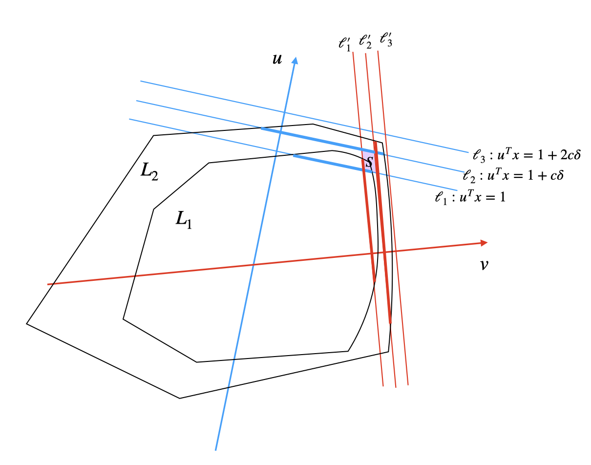
Figure 2: The intersection of halfspaces has measure $O(\delta^{2})$.

∎

References

• [1] Sanjeev Arora, Rong Ge, Ankur Moitra, and Sushant Sachdeva. Provable ICA with unknown gaussian noise, with implications for gaussian mixtures and autoencoders. In NIPS, pages 2384–2392, 2012.
• [2] Ainesh Bakshi, Ilias Diakonikolas, He Jia, Daniel M Kane, Pravesh K Kothari, and Santosh S Vempala. Robustly learning mixtures of k arbitrary gaussians. In Proceedings of the 54th Annual ACM SIGACT Symposium on Theory of Computing, pages 1234–1247, 2022.
• [3] Ainesh Bakshi and Adarsh Prasad. Robust linear regression: Optimal rates in polynomial time. In Proceedings of the 53rd Annual ACM SIGACT Symposium on Theory of Computing, pages 102–115, 2021.
• [4] Keith Ball. Cube slicing in rn. Proceedings of the American Mathematical Society, pages 465–473, 1986.
• [5] Franck Barthe and Alexander Koldobsky. Extremal slabs in the cube and the laplace transform. Advances in Mathematics, 174(1):89–114, 2003.
• [6] Mikhail Belkin, Luis Rademacher, and James Voss. Blind signal separation in the presence of Gaussian noise. In Proc. of COLT, 2013.
• [7] J-F Cardoso. Multidimensional independent component analysis. In Acoustics, Speech and Signal Processing, 1998. Proceedings of the 1998 IEEE International Conference on, volume 4, pages 1941–1944. IEEE, 1998.
• [8] Y. Cheng, I. Diakonikolas, R. Ge, and D. P. Woodruff. Faster algorithms for high-dimensional robust covariance estimation. In Conference on Learning Theory, COLT 2019, pages 727–757, 2019.
• [9] P. Comon. Independent Component Analysis. In Proc. Int. Sig. Proc. Workshop on Higher-Order Statistics, pages 111–120, Chamrousse, France, July 10-12 1991. Keynote address. Republished in Higher-Order Statistics, J.L.Lacoume ed., Elsevier, 1992, pp 29–38.
• [10] Pierre Comon and Christian Jutten, editors. Handbook of Blind Source Separation. Academic Press, 2010.
• [11] I. Diakonikolas, G. Kamath, D. M. Kane, J. Li, A. Moitra, and A. Stewart. Robust estimators in high dimensions without the computational intractability. In Proc. 57th IEEE Symposium on Foundations of Computer Science (FOCS), pages 655–664, 2016.
• [12] A. Frieze, M. Jerrum, and R. Kannan. Learning linear transformations. In focs1996, pages 359–368, 1996.
• [13] N. Goyal, S. Vempala, and Y. Xiao. Fourier pca and robust tensor decomposition. In Proceedings of the forty-sixth annual ACM symposium on Theory of computing, pages 584–593, 2014.
• [14] A. Klivans, P. Kothari, and R. Meka. Efficient algorithms for outlier-robust regression. In Proc. 31st Annual Conference on Learning Theory (COLT), pages 1420–1430, 2018.
• [15] P. K. Kothari, J. Steinhardt, and D. Steurer. Robust moment estimation and improved clustering via sum of squares. In Proc. 50th Annual ACM Symposium on Theory of Computing (STOC), pages 1035–1046, 2018.
• [16] P. K. Kothari and D. Steurer. Outlier-robust moment-estimation via sum-of-squares. CoRR, abs/1711.11581, 2017.
• [17] K. A. Lai, A. B. Rao, and S. Vempala. Agnostic estimation of mean and covariance. In Proc. 57th IEEE Symposium on Foundations of Computer Science (FOCS), pages 665–674, 2016.
• [18] L. Lovász and S. Vempala. The geometry of logconcave functions and sampling algorithms. Random Structures and Algorithms, 30(3):307–358, 2007.
• [19] Phong Q. Nguyen and Oded Regev. Learning a parallelepiped: Cryptanalysis of GGH and NTRU signatures. J. Cryptology, 22(2):139–160, 2009.