ZoeDepth: Zero-shot Transfer by Combining Relative and Metric Depth

Abstract

This paper tackles the problem of depth estimation from a single image. Existing work either focuses on generalization performance disregarding metric scale, i.e. relative depth estimation, or state-of-the-art results on specific datasets, i.e. metric depth estimation. We propose the first approach that combines both worlds, leading to a model with excellent generalization performance while maintaining metric scale. Our flagship model, ZoeD-M12-NK, is pre-trained on 12 datasets using relative depth and fine-tuned on two datasets using metric depth. We use a lightweight head with a novel bin adjustment design called metric bins module for each domain. During inference, each input image is automatically routed to the appropriate head using a latent classifier. Our framework admits multiple configurations depending on the datasets used for relative depth pre-training and metric fine-tuning. Without pre-training, we can already significantly improve the state of the art (SOTA) on the NYU Depth v2 indoor dataset. Pre-training on twelve datasets and fine-tuning on the NYU Depth v2 indoor dataset, we can further improve SOTA for a total of 21% in terms of relative absolute error (REL). Finally, ZoeD-M12-NK is the first model that can jointly train on multiple datasets (NYU Depth v2 and KITTI) without a significant drop in performance and achieve unprecedented zero-shot generalization performance to eight unseen datasets from both indoor and outdoor domains. The code and pre-trained models are publicly available at https://github.com/isl-org/ZoeDepth.

Figure 2: ZoeDepth architecture. An RGB image is fed into the MiDaS depth estimation framework [33]. The bottleneck and succeeding four hierarchy levels of the MiDaS decoder (at $1/32$, $1/16$, $1/8$, $1/4$ and $1/2$ of the MiDaS in- and output resolution) are hooked into the metric bins module (see Fig. 3). The metric bins module computes the per-pixel depth bin centers that are linearly combined to output the metric depth. Different transformer backbones can be utilized for the MiDaS encoder; a state-of-the-art example is BEiT₃₈₄-L [3].

1 Introduction

Single-image depth estimation (SIDE) is a classic problem in computer vision with many recent contributions. There are two branches of work: metric depth estimation (MDE) and relative depth estimation (RDE). The dominant branch is MDE [5, 6, 50, 26, 30], where the goal is to estimate depth in absolute physical units, i.e. meters. The advantage of predicting metric depth is the practical utility for many downstream applications in computer vision and robotics, such as mapping, planning, navigation, object recognition, 3D reconstruction, and image editing. However, training a single metric depth estimation model across multiple datasets often deteriorates the performance, especially when the collection includes images with large differences in depth scale, e.g. indoor and outdoor images. As a result, current MDE models usually overfit to specific datasets and do not generalize well to other datasets.

The second branch of work, relative depth estimation [30, 33], deals with the large depth scale variation in multiple types of environments by factoring out the scale. As a result, disparity is sufficient for supervision; metric scale and camera parameters are not required and do not need to be consistent across datasets. In RDE, depth predictions per pixel are only consistent relative to each other across image frames and the scale factor is unknown. This allows methods to be trained on a diverse set of scenes and datasets, even 3D movies [33], enabling model generalizability across domains. The trade-off is that the predicted depth has no metric meaning, limiting the applications.

In this paper, we propose a two-stage framework that combines the two approaches (see Fig. 2). In the first stage, we train a common encoder-decoder architecture for relative depth estimation using the standard training scheme [32]. Our model first learns from a large variety of datasets in pre-training which leads to good generalization. In the second stage, we add heads for metric depth estimation to the encoder-decoder architecture and fine-tune them on metric depth datasets, using one light-weight metric head per domain (a metric had has less than 1% of the parameters of the backbone). During inference, an image is automatically routed to the appropriate head using a classifier on encoder features. Adding these domain-specific heads helps the model learn metric depth while benefiting from the relative depth pre-training. Our metric head design (dubbed metric bins module) is inspired by a recently introduced method for metric depth estimation [6] that estimates a set of depth values instead of a single depth value per pixel. Similarly, we estimate a set of depth values (bins) and subsequently transform this estimation at each layer of the decoder using a novel concept we call attractors.

Our framework is flexible and can be used in multiple different configurations. We specifically want to highlight three configurations, that improve the state-of-the-art (SOTA) in different categories of metric SIDE. These three configurations are the main contributions of this paper.

Metric SIDE. Without any relative pre-training, our model ZoeD-X-N is trained only on NYU Depth v2 [37]. This configuration validates the design of our metric bins module and demonstrates that it can already improve upon the current SOTA NeWCRFs [50] by 13.7% on indoor depth estimation without relative depth pre-training.

Metric SIDE with relative depth pre-training. By conducting relative depth pre-training on 12 datasets and then conducting metric fine tuning on NYU Depth v2, our model ZoeD-M12-N can further improve on ZoeD-X-N by 8.5%, leading to 21% improvement over current published SOTA. Existing architectures do not have an established way to benefit from relative depth pre-training at a competitive level.

Universal Metric SIDE with automatic routing. We make a step towards universal depth estimation in the wild. Our flagship architecture ZoeD-M12-NK uses relative pre-training on 12 datasets combined with metric fine-tuning on indoor and outdoor datasets, i.e. NYU Depth v2 and KITTI, jointly. We evaluate this setup by first showing that it significantly outperforms SOTA on datasets it was trained on (NYU and KITTI) when compared to other models that are also trained on these two datasets jointly; we achieve an overall improvement in absolute relative error (REL) of 24.3%. Second, our setup outperforms SOTA on 7 metric datasets it was not trained on, with up to 976.4% ($\sim$11x) improvement in metrics; this demonstrates its unprecedented zero-shot capabilities.

2 Related Work

2.1 Single-Image Depth Estimation (SIDE)

Supervised single-image depth estimation methods can be categorized into regressing metric depth [30, 16, 5, 6, 50, 26] and relative depth [21, 33, 32, 30]. Metric depth models are typically trained on singular datasets, are more prone to overfitting, and typically generalize poorly to unseen environments or across varying depth ranges. Relative depth models tend to generalize better as they can be trained on more diverse datasets with relative depth annotations using scale-invariant losses. Yet, their utility for downstream tasks requiring metric depth is limited, as relative depth models regress depth with unknown scale and shift. Recent works have sought to resolve metric information in regressed depth. For example, Yin et al. [49] recover 3D scene shape from a single image via a two-stage framework combining monocular depth estimation with 3D point cloud encoders that are trained to predict missing depth shift and focal length. Jun et al. [16] decompose metric depth into normalized depth and scale features and propose a multi-decoder network where a metric depth decoder leverages relative depth features from the gradient and normalized depth decoders. Universal depth prediction has also been investigated by the Robust Vision Challenge  that includes indoor and outdoor domains. A popular idea is to discretize the target depth interval and reformulate the continuous depth regression as a classification task [11, 24, 23, 34]. Ren et al. [34] propose a two-stage framework: first involving training a classifier to distinguish low-depth-range and high-depth-range images. Two separate networks are then trained for the respective depth ranges. We compare to the best publicly available model based on DORN [11].

2.2 Distribution learning for metric SIDE

Many conventional learning-based monocular depth estimation methods adopt encoder-decoder architectures with convolutional layers, and more recently, transformer blocks. Depth estimation is commonly treated as a per-pixel regression task. An evolving line of work seeks to reformulate depth estimation as a combined classification-regression problem that reasons about distributions of depth values across an image. AdaBins [5] extends standard encoder-decoder backbones with a transformer-based module that discretizes predicted depth ranges into bins, where bin widths are determined adaptively per image; the final depth estimation is computed as a linear combination of bin centers. LocalBins [6] builds on this concept by considering depth distributions within local neighborhoods of a given pixel instead of globally over the image, as well as computing bin embeddings in a multi-scale fashion across decoder layers. PixelBins [36] simplifies AdaBins by replacing transformer block with convolutions, reducing complexity. BinsFormer [26] incorporates an auxiliary scene classification query to guide bin generation and also utilizes a multi-scale strategy to refine adaptively-generated bins. PixelFormer [2] treats depth estimation as pixel queries that are refined via skip attention and that are used to predict bin centers without leveraging decoded features.

3 Methodology

In this section, we describe our architecture, design choices and training protocol in detail.

3.1 Overview

We use the MiDaS [33] training strategy for relative depth prediction. MiDaS uses a loss that is invariant to scale and shift. If multiple datasets are available, a multi-task loss that ensures pareto-optimality across the datasets is used. The MiDaS training strategy can be applied to many different network architectures. We use the DPT encoder-decoder architecture as our base model [32], but replace the encoder with more recent transformer-based backbones [3]. After pre-training the MiDaS model for relative depth prediction, we add one or more heads for metric depth estimation by attaching our proposed metric bins module to the decoder (see Fig. 2 for the overall architecture). The metric bins module outputs metric depth and follows the adaptive binning principle, originally introduced in [5] and subsequently modified by [6, 26, 2, 36]. In particular, we start out with the pixel-wise prediction design as in LocalBins [6] and propose modifications that further improve performance. Finally, we fine-tune the complete architecture end-to-end.

3.2 Architecture Details

We first review LocalBins, and then introduce our novel metric bins module with attractor layers, our bin aggregation strategy, and loss function.

LocalBins review.

Our metric bins module is inspired by the LocalBins architecture proposed in [6]. LocalBins uses a standard encoder-decoder as the base model and attaches a module that takes the multi-scale features from the encoder-decoder as input and predicts the bin centers at every pixel. Final depth at a pixel is obtained by a linear combination of the bin centers weighted by the corresponding predicted probabilities. The LocalBins module first predicts $N_{seed}$ different seed bins at each pixel position at the bottleneck. Each bin is then split into two at every decoder layer using splitter MLPs. The number of bin centers is doubled at every decoder layer and we end up with $2^{n}N_{seed}$ bins at each pixel at the end of $n$ decoder layers. Simultaneously, the probability scores (p) over $N_{total}=2^{n}N_{seed}$ bin centers (c) are predicted from the decoder features using softmax and the final depth at pixel $i$ is obtained using:

$$d(i)=\sum_{k=1}^{N_{total}}{p_{i}(k)c_{i}(k)}$$ (1)

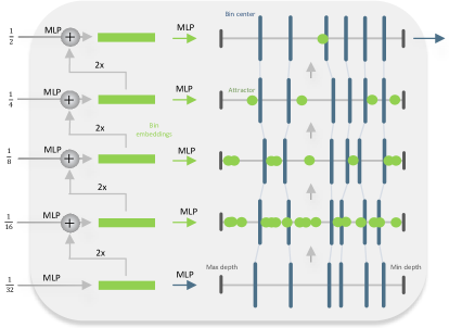
Figure 3: Metric Bins Module. Five incoming channels, corresponding to different depth hierarchies (see Fig. 2), are converted to 1-dimensional bin embeddings (green boxes) by MLPs, in combination with upsampling and addition operations. The lowest bin embedding yields metric bin centers (blue, vertical lines; not representative of actual number 64), whereas the remaining embeddings provide attractors for their respective hierarchy levels (green dots). Going upwards in the metric bins module, the attractors pull the bin centers according to Eqs. (2) and (3).

Metric bins module.

The metric bins module takes multi-scale features from the MiDaS decoder as input and predicts the bin centers to be used for metric depth prediction (see Fig. 3). However, instead of starting with a small number of bins at the bottleneck and splitting them later, our metric bins module predicts all the bin centers at the bottleneck and adjusts them at subsequent decoder layers. This bin adjustment is implemented via our newly proposed building block, called attractor layers.

Attract instead of split.

LocalBins implements multi-scale refinement of the bins by splitting them conditioned on the multi-scale features. In contrast, we implement the multi-scale refinement of the bins by adjusting them, moving them left or right on the depth interval. Using the multi-scale features, we predict a set of points on the depth interval towards which the bin centers get attracted. More specifically, at the $l^{th}$ decoder layer, an MLP takes the features at a pixel as input and predicts $n_{a}$ attractor points $\{a_{k}:k=1,...,n_{a}\}$ for that pixel position. The adjusted bin center is $c_{i}^{\prime}=c_{i}+\Delta c_{i}$, with the adjustment given by:

$$\Delta c_{i} =\sum_{k=1}^{n_{a}}\frac{a_{k}-c_{i}}{1+\alpha|a_{k}-c_{i}|^{\gamma}}$$ (2)

where the hyperparameters $\alpha$ and $\gamma$ determine the attractor strength. We name this attractor variant inverse attractor. We also experiment with an exponential variant given by:

$$\Delta c_{i} =\sum_{k=1}^{n_{a}}(a_{k}-c_{i})e^{-\alpha|a_{k}-c_{i}|^{\gamma}}$$ (3)

Our experiments suggest that the inverse attractor leads to better performance. We let the number of attractor points vary from one decoder layer to another, denoted together as a set $\{n^{l}_{a}\}$. We use $N_{total}=64$ bins and $\{16,8,4,1\}$ attractors. Please refer to Sec. 5.4 for various ablations.

The attracting strategy is preferred because it’s a contracting process while splitting is inherently dilative. Splitting adds extra constraints of newly produced bins summing up to the original bin width, while attractors adjust freely without such local constraints (only the total width is invariant). Intuitively, the prediction should get more refined and focused with decoder layers, which attractors achieve without dealing with any local constraints.

Log-binomial instead of softmax.

To get the final metric depth prediction, the bin centers are linearly combined, weighted by their probability scores as per Eq. (1). Prior adaptive bins based models [5, 6, 26, 2] use a softmax to predict the probability distribution over the bin centers. The choice of softmax is mainly inspired from the discrete classification analogy. Although the softmax plays well with unordered classes, since the bins are inherently ordered, it intuitively makes sense to use an ordering-aware prediction of the probabilities. The softmax approach can result in vastly different probabilities for nearby bin centers ($|p_{i}-p_{i+1}|>>0$). Inspired by Beckham and Pal [4], we use a binomial distribution instead to address this issue and correctly consider ordinal relationships between bins.

The binomial distribution has one parameter $q$ which controls the placement of the mode. We concatenate the relative depth predictions with the decoder features and predict a 2-channel output ($q$ - mode and $t$ - temperature) from the decoder features to get the probability score over the $k^{th}$ bin center by:

$$p(k;N,q)={N\choose k}q^{k}(1-q)^{N-k}$$ (4)

where $N=N_{total}$ is the total number of bins. In practice, since we use large values of $N$, we take $\log{(p)}$, use Stirling’s approximation [1] for factorials and apply $\text{softmax}(\{\log{(p_{k})}/t\}_{k=1}^{N})$ to get normalized scores for numerical stability. The parameter $t$ controls the temperature of the resulting distribution. The softmax normalization preserves the unimodality of the logits. Finally, the resulting probability scores and the bin centers from the metric bins module are used to obtain the final depth as per Eq. (1).

Loss.

We use the scale-invariant log loss ($\mathcal{L}_{pixel}$) for pixel-level supervision as in LocalBins [6]. Unlike LocalBins, we do not use the chamfer loss for bins due to the high memory requirement but only limited improvement.

3.3 Training strategies

As described previously, we have two stages for training: relative depth pre-training for the MiDaS backbone and metric depth fine-tuning for the prediction heads. We compare models with and without pre-training for relative depth as in [33]. We also explore different variations of fine-tuning, using a single dataset and multiple datasets; in the case of multiple datasets, we also compare using a single head, i.e. metric bins module, to using multiple heads. Please refer to Sec. 4.2 for more details about the exact model definitions. In the supplement, we report results for additional variations.

Metric fine-tuning on multiple datasets

Training a metric depth model on a mixture of datasets with a wide variety of scenes, for example from indoor and outdoor domains, is hard. The model not only has to handle images taken with different cameras and camera settings but also has to learn to adjust for the large variations in the overall scale of the scenes. Indoor scenes are usually limited to a maximum depth of 10 meters while outdoor scenes can have infinite depth (capped at 80 meters in most prior works). We hypothesize that a backbone pre-trained for relative depth estimation, alleviates the issues of fine-tuning on multiple datasets to some extent. We can also equip the model with multiple metric bins modules, one for each scene type (indoor versus outdoor). Different metric heads can be thought of as scene-type experts. Note that the base model is still common to all metric heads; the complete model with multiple heads is trained end-to-end. See Sec. 5.2 for a comparison of our model with single head and multiple heads.

Routing to metric heads.

When the model has multiple metric heads, we need a router that chooses the metric head to use for a particular input. We employ commonly used routing mechanisms developed in other contexts, e.g., see Fedus et al. [10] for a review. We explore three main variants: (R.1) Labeled Router: In this variant, we provide scene type labels (indoor or outdoor) to the model at both training and inference times and manually map from the scene type to the metric head. (R.2) Trained Router: Here, we train a classifier MLP that predicts the scene type of the input image based on the bottleneck features and then routes to the corresponding metric head. Therefore, this variant only needs scene-type labels during training. (R.3) Auto Router: In this setting, a router MLP (equivalent to a classifier in R.2) is used, but no labels are provided during either training or inference. Both the trainable router types, Trained Router and Auto Router, are trained end-to-end with the whole model. See Sec. 5.4 for a performance comparison of the discussed routing mechanisms.

4 Experimental Setup

4.1 Datasets

Our primary datasets for training ZoeDepth are NYU Depth v2 (N) for indoor and KITTI (K) for outdoor scenes. We refer to the combination of both datasets as (NK). For pre-training the relative depth backbone, we train on a mix of 12 datasets (M12) consisting of the 10 datasets used in [32]: HRWSI [46], BlendedMVS [47], ReDWeb [45], DIML-Indoor [17], 3D Movies [33], MegaDepth [25], WSVD [41], TartanAir [43], ApolloScape [15] and IRS [42], plus 2 additional datasets: KITTI [29] and NYU Depth v2 [37].

To demonstrate generalizability, we evaluate zero-shot performance on a number of real-world and synthetic datasets: SUN RGB-D [38], iBims [18], DIODE Indoor [40] and HyperSim  [35] for the indoor domain; DDAD [12], DIML Outdoor [17], DIODE Outdoor [40] and Virtual KITTI 2 [7] for the outdoor domain. We provide further details about the datasets in the supplement.

\begin{overpic}[scale={.25},width=390.25534pt]{figures/nyu_comparison_nrows3.png} \put(6.0,-2.0){Input} \put(19.0,-2.0){Ground Truth} \put(35.0,-2.0){NeWCRFs~{}\cite[cite]{[\@@bibref{}{yuan2022new}{}{}]}} \put(55.0,-2.0){Ours} \put(70.0,-2.0){NeWCRFs $\Delta$} \put(87.0,-2.0){Ours $\Delta$} \par\end{overpic}

Figure 4: Qualitative comparison on NYU Depth v2. Our method consistently produces better predictions with much less error. When looking closely at the depth maps it can also be observed that our predictions are much sharper with clear edges. $\Delta$ indicates square error ranging from lowest (dark blue) to highest (dark red) across predictions. Invalid regions are indicated as grey.

4.2 Models

The models are named according to the following convention: ZoeD-{RDPT}-{MFT}, where ZoeD is the abbreviation for ZoeDepth, RDPT denotes the datasets used for relative depth pre-training (X denotes no pre-training) and MFT denotes the datasets used for metric depth fine-tuning. We train and evaluate the following models: ZoeD-X-N, ZoeD-X-K, ZoeD-M12-N, ZoeD-M12-K and ZoeD-M12-NK. All models use the BEiT₃₈₄-L backbone from timm [44] that was pre-trained on ImageNet. The models ZoeD-X-N and ZoeD-X-K are directly fine-tuned for metric depth on NYU Depth v2 and KITTI respectively without any pre-training for relative depth estimation. ZoeD-M12-N and ZoeD-M12-K additionally include pre-training for relative depth estimation on the M12 dataset mix before the fine-tuning stage for metric depth. ZoeD-M12-NK is also pre-trained on M12, but has two separate heads fine-tuned on both NYU Depth v2 and KITTI. ZoeD-M12-NK^† is a variant of this model with a single head but otherwise the same pre-training and fine-tuning procedure. In the supplement, we provide further results for models trained on additional dataset combinations in pre-training and fine-tuning.

4.3 Evaluation Metrics

We evaluate in metric depth space $\mathbf{d}$ by computing the absolute relative error (REL) $=\frac{1}{M}\sum_{i=1}^{\put(0.0,-3.0){\scriptsize{$M$}}}|\mathbf{d}_{i}-\hat{\mathbf{d}}_{i}|/\mathbf{d}_{i}$, the root mean squared error (RMSE) $=[\frac{1}{M}\sum_{i=1}^{\put(0.0,-3.0){\scriptsize{$M$}}}|\mathbf{d}_{i}-\hat{\mathbf{d}}_{i}|^{2}]^{\frac{1}{2}}$, the average $\log_{10}$ error $=\frac{1}{M}\sum_{i=1}^{\put(0.0,-3.0){\scriptsize{$M$}}}|\log_{10}{\mathbf{d}_{i}}-\log_{10}{\hat{\mathbf{d}}_{i}}|$, and the threshold accuracy $\delta_{n}=\%$ of pixels s.t. $\max{(\mathbf{d}_{i}/\hat{\mathbf{d}}_{i},\hat{\mathbf{d}}_{i}/\mathbf{d}_{i})}<1.25^{n}$ for $n=1,2,3$, where $\mathbf{d}_{i}$ and $\hat{\mathbf{d}}_{i}$ refer to ground truth and predicted depth at pixel $i$, respectively, and $M$ is the total number of pixels in the image. We cap the evaluation depth at 10m for indoor datasets (8m for SUN RGB-D) and at 80m for outdoor datasets. Final model outputs are computed as the average of an image’s depth prediction and the prediction of its mirror image and are evaluated at ground truth resolution.

In addition, we define two metrics to measure relative improvement (RI) across datasets and metrics respectively. For $M$ datasets $D_{i}$ with $i\in{[1,M]}$, we compute $\text{mRI}_{D}=\frac{1}{M}\sum_{i=1}^{M}\text{RI}_{D_{i}}$. Similarly, for $N$ metrics $\theta_{j}$ with $j\in{[1,N]}$, we compute $\text{mRI}_{\theta}=\frac{1}{N}\sum_{j=1}^{N}\text{RI}_{\theta_{i}}$. For metrics where lower is better, $\text{RI}=\frac{r-t}{r}$ and for metrics where higher is better $\text{RI}=\frac{t-r}{r}$, where $r$ and $t$ correspond to the reference and target scores respectively.

5 Results

5.1 Comparison to SOTA on NYU Depth V2

Method	$\delta_{1}$$\uparrow$	$\delta_{2}$$\uparrow$	$\delta_{3}$ $\uparrow$	REL $\downarrow$	RMSE $\downarrow$	$\log_{10}$ $\downarrow$
Eigen et al. [9]	0.769	0.950	0.988	0.158	0.641	–
Laina et al. [19]	0.811	0.953	0.988	0.127	0.573	0.055
Hao et al. [13]	0.841	0.966	0.991	0.127	0.555	0.053
DORN [11]	0.828	0.965	0.992	0.115	0.509	0.051
SharpNet [31]	0.836	0.966	0.993	0.139	0.502	0.047
Hu et al. [14]	0.866	0.975	0.993	0.115	0.530	0.050
Lee et al. [22]	0.837	0.971	0.994	0.131	0.538	–
Chen et al. [8]	0.878	0.977	0.994	0.111	0.514	0.048
BTS [20]	0.885	0.978	0.994	0.110	0.392	0.047
Yin et al. [48]	0.875	0.976	0.994	0.108	0.416	0.048
AdaBins [5]	0.903	0.984	0.997	0.103	0.364	0.044
LocalBins [6]	0.907	0.987	0.998	0.099	0.357	0.042
Jun et al. [16]	0.913	0.987	0.998	0.098	0.355	0.042
NeWCRFs [50]	0.922	0.992	0.998	0.095	0.334	0.041
ZoeD-X-N	0.946	0.994	0.999	0.082	0.294	0.035
ZoeD-M12-N	0.955	0.995	0.999	0.075	0.270	0.032
ZoeD-M12-NK	0.953	0.995	0.999	0.077	0.277	0.033

Table 1: Quantitative comparison on NYU-Depth v2. The reported numbers of prior art are from the corresponding original papers. Best results are in bold, second best are underlined.

Our novel architecture beats SOTA without using any additional data for pre-training. To demonstrate this, we evaluate our model ZoeD-X-N on the popular metric depth estimation benchmark NYU Depth v2 [37]. ZoeD-X-N is not pre-trained for relative depth; the backbone is initialized with the standard weights from ImageNet pre-training. Tab. 1 shows the performance of models on the official NYU Depth v2 test set. This model already outperforms NeWCRFs [50] by 13.7% (REL = 0.082), highlighting the contribution of our architecture design.

Next, we verify that our architecture can benefit from relative depth pre-training. Our corresponding model ZoeD-M12-N significantly outperforms the prior state-of-the-art NeWCRFs [50] by nearly 21% (REL = 0.075). Results are not just numerically better; the resulting depth maps also have much sharper boundaries (see Fig. 4). We believe this is the first demonstration of successful relative depth pre-training at a competitive level. While other architectures can also benefit from pre-training, some modifications are required. In the next section, we show one such modification by combining our base model with architecture building blocks proposed by other papers (see Tab. 2). This shows that while other architectures benefit from our larger backbone and relative depth pre-training, they are still not competitive with our complete framework.

5.2 Universal Metric SIDE

Here, we evaluate our progress towards a universal metric depth estimation framework by analyzing our model ZoeD-M12-NK which was trained across two different metric datasets and generalizes across indoor and outdoor domains. Models trained across multiple metric datasets usually perform worse or diverge. In contrast, our model ZoeD-M12-NK still outperforms the previous SOTA NeWCRFs [50] on NYU Depth v2 by 18.9% (REL = 0.077, Tab. 1). While ZoeD-M12-NK is not as good as our model (ZoeD-M12-N) fine-tuned only on NYU Depth v2, it provides a very attractive trade-off between performance and generalization across domains.

To underline the difficulty of cross-domain training, we perform a comparison to other models trained simultaneously on indoor and outdoor datasets (NK). First, we evaluate recent methods trained on NK without any architectural modifications and compare them with our method in Tab. 2. We find that existing works are unable to achieve competitive results in that setting. AdaBins [5] and PixelBins [36] fail to converge at all, while the SOTA NeWCRFs’ [50] performance degrades by nearly 15% (REL 0.095 to 0.109) on NYU (compare Tab. 2 with Tab. 1). These experiments confirm that previous models significantly degrade when being trained jointly on datasets from different domains. In contrast, we only observe an 8% drop (REL 0.075 to 0.081) while using the shared head, demonstrating our model’s ability to deal with different domains at once. This gap is further reduced to mere 2.6% (REL 0.075 vs 0.077) using our two-head model ZoeD-M12-NK, outperforming NeWCRFs [50] by 25.2% (mRI_D in REL).

Method	NYU	KITTI	iBims-1	vKITTI-2	mRID
Baselines: no modification
DORN$\text{-X-NK}^{\dagger}$	0.156	0.115	0.287	0.259	-45.7%
LocalBins$\text{-X-NK}^{\dagger}$	0.245	0.133	0.296	0.265	-74.0%
PixelBins$\text{-X-NK}^{\dagger}$	-	-	-	-	-
NeWCRFs$\text{-X-NK}^{\dagger}$	0.109	0.076	0.189	0.190	0.0%
Baselines: modified to use our pre-trained DPT-BEiT-L as backbone
DORN$\text{-M12-NK}^{\dagger}$	0.110	0.081	0.242	0.215	-12.2%
LocalBins$\text{-M12-NK}^{\dagger}$	0.086	0.071	0.221	0.121	11.8%
PixelBins$\text{-M12-NK}^{\dagger}$	0.088	0.071	0.232	0.119	10.1%
NeWCRFs$\text{-M12-NK}^{\dagger}$	0.088	0.073	0.233	0.124	8.7%
Ours: different configuations for fair comparison
$\text{ZoeD-X-NK}^{\dagger}$	0.095	0.074	0.187	0.184	4.9%
$\text{ZoeD-M12-NK}^{\dagger}$	0.081	0.061	0.210	0.112	18.8%
ZoeD-M12-NK	0.077	0.057	0.186	0.105	25.2%

Table 2: Comparison with existing works when trained on NYU and KITTI. Results are reported using the REL metric. The mRI_D column denotes the mean relative improvement with respect to NeWCRFs across datasets. X in the model name, means no architecture change and no pre-training. M12 means that the model was pre-trained (using our base model based on the DPT architecture with the BEiT-L encoder). All models are fine-tuned on NYU and KITTI. $\dagger$ denotes a single metric head (shared); single-head training allows us to adapt prior models without major changes. Best results are in bold, second best are underlined. PixelBins [36] did not converge without modification. We also tried to train AdaBins [5] across both datasets, but despite our best effort and extensive hyperparameter tuning, it did not converge.

We conclude that previous models require changes to successfully train on multiple datasets. We conduct additional experiments where we improve previous models by incorporating part of our framework. Specifically, we use the same base model (DPT with a BEiT-L backbone), with relative pre-training on M12, and with fine-tuning on NK (NYU and KITTI mixture) using a single metric head; only the design of the metric head varies. Tab. 2 shows that previous models still fall behind in this setting. Since DORN [11] and LocalBins [6] are light-weight and modular, they can be easily used in conjuction with our pre-trained relative depth model instead of our metric bins module. NeWCRFs [50] is originally a tightly-coupled decoder-focused design; however, to keep the base model exactly the same, we use an extra head with NeWCRFs layers that use DPT decoder features as multi-scale input. This increases the complexity significantly ($\sim$40M more parameters than ours) yet still underperforms when compared to pixel-wise bins-based methods: LocalBins, PixelBins and ZoeD-M12-NK. This suggests that bins-based architectures are better suited for multi-domain training and can better exploit relative depth pre-training. Our model performs best both on NYU and KITTI, as well as on iBims-1 and virtual KITTI-2 that have not been seen in training. These results indicate that our metric bins module exploits pre-training better than existing works, enabling improved domain adaptation and generalization (zero-shot performance). We investigate zero-shot performance in more detail next.

	SUN RGB-D				iBims-1 Benchmark				DIODE Indoor				HyperSim
Method	$\delta_{1}$ $\uparrow$	REL $\downarrow$	RMSE $\downarrow$	mRIθ $\uparrow$	$\delta_{1}$ $\uparrow$	REL $\downarrow$	RMSE $\downarrow$	mRIθ $\uparrow$	$\delta_{1}$ $\uparrow$	REL $\downarrow$	RMSE $\downarrow$	mRIθ $\uparrow$	$\delta_{1}$ $\uparrow$	REL $\downarrow$	RMSE $\downarrow$	mRIθ $\uparrow$
BTS [20]	0.740	0.172	0.515	-14.2%	0.538	0.231	0.919	-6.9%	0.210	0.418	1.905	2.3%	0.225	0.476	6.404	-8.6%
AdaBins [5]	0.771	0.159	0.476	-7.0%	0.555	0.212	0.901	-2.1%	0.174	0.443	1.963	-7.2%	0.221	0.483	6.546	-10.5%
LocalBins [6]	0.777	0.156	0.470	-5.6%	0.558	0.211	0.880	-0.7%	0.229	0.412	1.853	7.1%	0.234	0.468	6.362	-6.6%
NeWCRFs [50]	0.798	0.151	0.424	0.0%	0.548	0.206	0.861	0.0%	0.187	0.404	1.867	0.0%	0.255	0.442	6.017	0.0%
ZoeD-X-N	0.857	0.124	0.363	13.2%	0.668	0.173	0.730	17.7%	0.400	0.324	1.581	49.7%	0.284	0.421	5.889	6.1%
ZoeD-M12-N	0.864	0.119	0.346	16.0%	0.658	0.169	0.711	18.5%	0.376	0.327	1.588	45.0%	0.292	0.410	5.771	8.6%
ZoeD-M12-NK	0.856	0.123	0.356	13.9%	0.615	0.186	0.777	10.6%	0.386	0.331	1.598	46.3%	0.274	0.419	5.830	5.3%

Table 3: Quantitative results for zero-shot transfer to four unseen indoor datasets. mRI_θ denotes the mean relative improvement with respect to NeWCRFs across all metrics ($\delta_{1}$, REL, RMSE). Evaluation depth is capped at 8m for SUN RGB-D, 10m for iBims and DIODE Indoor, and 80m for HyperSim. Best results are in bold, second best are underlined.

	Virtual KITTI 2				DDAD				DIML Outdoor				DIODE Outdoor
Method	$\delta_{1}$ $\uparrow$	REL $\downarrow$	RMSE $\downarrow$	mRIθ $\uparrow$	$\delta_{1}$ $\uparrow$	REL $\downarrow$	RMSE $\downarrow$	mRIθ $\uparrow$	$\delta_{1}$ $\uparrow$	REL $\downarrow$	RMSE $\downarrow$	mRIθ $\uparrow$	$\delta_{1}$ $\uparrow$	REL $\downarrow$	RMSE $\downarrow$	mRIθ $\uparrow$
BTS [20]	0.831	0.115	5.368	2.5%	0.805	0.147	7.550	-17.8%	0.016	1.785	5.908	24.3%	0.171	0.837	10.48	-4.8%
AdaBins [5]	0.826	0.122	5.420	0.0%	0.766	0.154	8.560	-26.7%	0.013	1.941	6.272	9.7%	0.161	0.863	10.35	-7.2%
LocalBins [6]	0.810	0.127	5.981	-5.3%	0.777	0.151	8.139	-23.2%	0.016	1.820	6.706	19.5%	0.170	0.821	10.27	-3.6%
NeWCRFs [50]	0.829	0.117	5.691	0.0%	0.874	0.119	6.183	0.0%	0.010	1.918	6.283	0.0%	0.176	0.854	9.228	0.0%
ZoeD-X-K	0.837	0.112	5.338	3.8%	0.790	0.137	7.734	-16.6%	0.005	1.756	6.180	-13.3%	0.242	0.799	7.806	19.8%
ZoeD-M12-K	0.864	0.100	4.974	10.5%	0.835	0.129	7.108	-9.3%	0.003	1.921	6.978	-27.1%	0.269	0.852	6.898	26.1%
ZoeD-M12-NK	0.850	0.105	5.095	7.8%	0.824	0.138	7.225	-12.8%	0.292	0.641	3.610	976.4%	0.208	0.757	7.569	15.8%

Table 4: Quantitative results for zero-shot transfer to four unseen outdoor datasets. mRI_θ denotes the mean relative improvement with respect to NeWCRFs across all metrics ($\delta_{1}$, REL, RMSE). Best results are in bold, second best are underlined.

5.3 Zero-shot Generalization

We evaluate the generalization capabilities of our approach by comparing its zero-shot performance to prior works on eight unseen indoor and outdoor datasets without fine-tuning; we show qualitative results in Fig. 1 and report quantitative results in Tab. 3 and Tab. 4.

Tab. 3 reports zero-shot generalization on indoor datasets. Even with fine-tuning across both the indoor (NYU Depth v2) and outdoor (KITTI) domains, our model ZoeD-M12-NK demonstrates significantly better performance than previous state-of-the-art models. The mean relative improvement (mRI_θ) ranges from 5.3% for HyperSim to 46.3% for DIODE Indoor. As expected, fine-tuning only on NYU Depth v2 so that the training and test domains are both indoor, i.e. ZoeD-M12-N, leads to an increase in mRI_θ on all datasets. ZoeD-X-N scores lower in most datasets due to the lack of relative depth pre-training.

Tab. 4 reports zero-shot generalization on outdoor datasets. Similar as for the indoor datasets, pre-training on M12 is generally beneficial. ZoeD-M12-NK improves from 7.8% for Virtual KITTI 2 to 976.4% for DIML Outdoor over NeWCRFs [50]. On DDAD, ZoeD-M12-NK performs 12.8% worse while NeWCRFs [50] is best. The metrics in Tab. 4 and the rightmost image in Fig. 1 show the quality of our results. Overall, our framework is the top performer in 7 out of 8 datasets.

Probably the most interesting result is the high $\text{mRI}_{\theta}$ value of 976.4% that ZoeD-M12-NK achieves on DIML Outdoor. All other models are fine-tuned only on KITTI with large depth ranges but the DIML Outdoor dataset contains mainly close-up images of outdoor scenarios making it more similar to an indoor dataset. Since ZoeD-M12-NK was also fine-tuned on NYU Depth v2 and automatically routes inputs to different heads, it seems to leverage its knowledge of the indoor domain to improve predictions. This is also supported by the low performance of ZoeD-X-K and ZoeD-M12-K which were only fine-tuned on KITTI. This result clearly shows the benefit of models fine-tuned across multiple domains for generalization to arbitrary datasets. We expect that defining more granular domains and fine-tuning a variant of our model with more than two heads across many metric datasets would lead to even better generalization performance.

5.4 Ablation Studies

In this section we study the importance of various design choices in our models.

Backbones.

We study the effect of using different backbones for our base MiDaS model. The results are summarized in Fig. 5. We find that larger backbones with more parameters lead to improved performance, but our model still outperforms the previous state of the art when using the same backbone [28]. Further, the image classification performance of the backbone is highly correlated to the performance of our depth estimation model, i.e. lower absolute relative error (REL). Hence, our architecture can directly benefit from new backbones as they get introduced in the future.

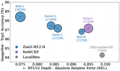
Figure 5: Backbone ablation study. There is a strong correlation between backbone performance in image classification and depth estimation. Larger backbones achieve lower absolute relative error (REL); with the same backbone and overall fewer parameters, our method still outperforms the current state-of-the-art NeWCRFs. The area of the circles is proportional to the number of parameters. The backbones shown are BEiT [3], Swin2 [27], Swin [28] and EfficientNet B5 [39], where L stands for large and B for base.

Metric head type			REL $\downarrow$	RMSE $\downarrow$
Type	Variant	Config
Naive head	-	-	0.096	0.335
Metric bins	Splitter	factor = 2	0.085	0.301
	Exponential Attractor	{16,8,4,1}	0.086	0.305
	Inverse Attractor	{8,8,8,8}	0.081	0.295
		{16,2,2,16}	0.081	0.291
		{1,4,8,16}	0.080	0.287
		{16,8,4,1}	0.075	0.270

Table 5: Metric head variants. The “Config” column specifies the split factor in case of the splitter variant and the number of attractors $\{n_{a}^{l}\}$ for attractor variants. The reported results are all based on ZoeD-M12-N evaluated on NYU Depth v2. Best results are in bold, second best are underlined.

Metric Bins Module.

We study the contribution to the overall performance by various variants of our metric bins module listed in Tab. 5. First, we remove our metric bins module and attach a convolutional block to the decoder features from the base DPT model and directly predict the metric depth (standard regression). We call this variant naive head. Our best attractor variant performs about 21% better than the naive head. Notably, the metric bins with the splitter design as in [6] improves upon the naive head by 11.4%, which is consistent with the 10.8% improvement observed by [6] when comparing a naive Unet design with the splitter LocalBins design (refer to Tab. 3 in [6]). Next, we compare our novel attractor design with the splitter design of LocalBins [6]. Our best attractor variant performs 11.7% better. All the inverse attractor variants perform decisively better than the splitter variant while the exponential variant performs slightly worse.

Routers.

As discussed in Sec. 3.3, we test the three variants for routing the relative features to metric heads. The results for the models with two metric heads, one for NYU Depth v2 and one for KITTI, are provided in Tab. 6. Out of the three variants, the Auto Router performs the worst. This is expected as in this case the router never sees any domain labels. Surprisingly, the Trained Router performs better on NYU Depth v2 than the Labeled Router, even though domain labels are unavailable during inference. We hypothesize that the domain-level discriminatory supervision may help in learning better representations. As we aim for a generic model without special requirements during inference, we choose the Trained Router and use it in all our multi-head models.

Log Binomial.

We evaluate the effect of using a log binomial distribution by studying the performance of ZoeD-M12-N on NYU-Depth-v2 with log binomial and softmax probability heads. Consistent with [4], we observe that using log binomial (REL = 0.075) instead of softmax (REL = 0.077) leads to about 2% improvement. This highlights the importance of unimodal distributions for ordinal problems.

	Labels required		REL $\downarrow$		RMSE $\downarrow$
Variant	Train	Inference	NYU	KITTI	NYU	KITTI
Labeled Router	✓	✓	0.080	0.057	0.290	2.452
Trained Router	✓	✗	0.077	0.057	0.277	2.362
Auto Router	✗	✗	0.102	0.075	0.377	2.584

Table 6: Router variants. The reported results are all based on ZoeD-M12-NK evaluated on NYU Depth v2 and KITTI. Best results are in bold, second best are underlined.

6 Conclusion

Our proposed framework, ZoeDepth, bridges the gap between relative and metric depth estimation. In the first stage, we pre-train an encoder-decoder architecture using relative depth on a collection of datasets. In the second stage, we add domain-specific heads based on our new metric bins module to the decoder and fine-tune the model on one or more datasets for metric depth prediction. Our proposed architecture decisively improves upon the state of the art for NYU Depth v2 (21% in REL) and also significantly improves upon the state of the art in zero-shot transfer. We expect that defining more granular domains beyond indoor and outdoor, and fine-tuning on more metric datasets can improve our results further. In future work, we would like to investigate a mobile architecture version of ZoeDepth, e.g., for on-device photo editing, and extend our work to stereo-image depth estimation.

Appendix A Appendix

A.1 Datasets Overview

We begin by providing a detailed overview of the properties of the datasets used for metric depth fine-tuning and evaluation of the new ZoeDepth architecture (see Fig. 2 in the main paper) in Table 7. These datasets consist of NYU Depth v2 [37] and KITTI [29] used for metric depth fine-tuning as well as respectively four in- and outdoor datasets to test for generalization performance (see Sec. 4.1 of the main paper). The indoor datasets consist of SUN RGB-D [38], the iBims benchmark [18], DIODE Indoor [40] and HyperSim  [35]. For the outdoor datasets, we use DDAD [12], DIML Outdoor [17], DIODE Outdoor [40] and Virtual KITTI 2 [7].

All ZoeDepth architectures and prior works are evaluated by resizing the input to the training resolution. Zoe-*-N, Zoe-*-NK, and Zoe-*-K models are trained at resolutions $384\times 512$, $384\times 512$ and $384\times 768$ respectively. Predictions are resized to original ground truth resolution before evaluation.

			Seen in	# Train	# Eval	Eval Depth [m]		Crop
Dataset	Domain	Type	Training?	Samples	Samples	Min	Max	Method
NYU Depth v2 [37]	Indoor	Real	✓	24k [20]	654	1e-3	10	Eigen
SUN RGB-D [38]	Indoor	Real	✗	-	5050	1e-3	8	Eigen
iBims-1 [18]	Indoor	Real	✗	-	100	1e-3	10	Eigen
DIODE Indoor [40]	Indoor	Real	✗	-	325	1e-3	10	Eigen
HyperSim [35]	Indoor	Synthetic	✗	-	7690	1e-3	80	Eigen
KITTI [29]	Outdoor	Real	✓	26k [20]	697	1e-3	80	Garg$\ddagger$
Virtual KITTI 2 [7]	Outdoor	Synthetic	✗	-	1701	1e-3	80	Garg$\ddagger$
DDAD [12]	Outdoor	Real	✗	-	3950	1e-3	80	Garg
DIML Outdoor [17]	Outdoor	Real	✗	-	500	1e-3	80	Garg
DIODE Outdoor [40]	Outdoor	Real	✗	-	446	1e-3	80	Garg

Table 7: Overview of datasets used in metric depth fine-tuning and evaluation of ZoeDepth architectures. For demonstrating zero-shot transfer, we evaluate across a total of 13165 indoor samples and 6597 outdoor samples. While HyperSim is predominantly an indoor dataset, there are several samples exhibiting depth ranges exceeding 10 m, so we relax the maximum evaluation depth up to 80 m. $\ddagger$ : To follow prior works [50, 5], we crop the sample and then use scaled Garg crop for evaluation. We verify the transforms by reproducing results obtained by using respective pre-trained checkpoints provided by prior works.

A.2 Training Details

In  Table 8, we show various training strategies (see Section 3.3 of the main paper) applied to the ZoeDepth architecture. The training strategies differ by the datasets used for relative depth pre-training of the MiDaS [33] encoder-decoder, the datasets employed for metric depth fine-tuning in ZoeDepth and the number of used metric heads. Each combination of these options provided in Tab. 8 defines a different model of ZoeDepth. Results for these combinations are shown in Section A.3.

Model	Relative depth pre-training	Metric depth fine-tuning	# metric heads
ZoeD-X-N	✗	NYU	1
ZoeD-N-N	NYU	NYU	1
ZoeD-NK-N	NYU+KITTI	NYU	1
ZoeD-M12-N	M12	NYU	1
ZoeD-X-K	✗	KITTI	1
ZoeD-K-K	KITTI	KITTI	1
ZoeD-NK-K	NYU+KITTI	KITTI	1
ZoeD-M12-K	M12	KITTI	1
ZoeD-NK-NK†	NYU+KITTI	NYU+KITTI	1
ZoeD-M12-NK†	M12	NYU+KITTI	1
ZoeD-NK-NK	NYU+KITTI	NYU+KITTI	2
ZoeD-M12-NK	M12	NYU+KITTI	2

Table 8: Models are named according to the following convention: ZoeD-RDPT-MFT, where ZoeD is the abbreviation for ZoeDepth, RDPT denotes the datasets used for relative depth pre-training and MFT denotes the datasets used for metric depth fine-tuning. Models with an X do not use a relative depth pre-training. The collection M12 contains the datasets HRWSI [46], BlendedMVS [47], ReDWeb [45], DIML-Indoor [17], 3D Movies [33], MegaDepth [25], WSVD [41], TartanAir [43], ApolloScape [15], IRS [42], KITTI (K) [29] and NYU Depth v2 (N) [37].

A.3 Detailed Results

In Tables 3 and 4 of the main paper, we have provided quantitative results for zero-shot transfer to the four in- and outdoor datasets unseen during training, which are mentioned in Section A.1. These results are supplemented by the threshold accuracies $\delta_{2}$ and $\delta_{3}$ as well as the average $\log_{10}$ error in Tables 9, 10, 11, 12, 13, 14, 15 and 16. Also, while the main paper only shows our models ZoeD-X-K, ZoeD-M12-K and ZoeD-M12-NK, Tables 9, 10, 11, 12, 13, 14, 15 and 16 contain the additional model ZoeD-NK-N. This model uses only the dataset combination of NYU Depth v2 (N) [37] and KITTI (K) [29] for the relative depth pre-training.

Figures 6, 7, 8, 9, 10, 11, 12 and 13 show metric depth maps computed with our ZoeDepth architecture for various example images of the in- and outdoor datasets described in Section A.1.

For the indoor datasets, NeWCRF shows a tendency to underestimate the depth, e.g., the relatively bright images of NeWCRF in rows 3 and 4 of Figure 6 as well as rows 1 and 3 of Figure 7. Our models Zoe-M12-NK and Zoe-M12-N are much closer to the ground truth. Only row 4 of Figure 9 is an exception where our models share this behavior with NeWCRF.

For the outdoor datasets, rows 1 to 3 of Figure 12 clearly demonstrate the advantage of our model ZoeD-M12-NK with respect to NeWCRF. As explained in Section 5.3 of the main paper, ZoeD-M12-NK is not only fine-tuned on the outdoor dataset KITTI but also on the indoor dataset NYU Depth v2, which better reflects the low depth values observable in the RGB and ground truth images of Figure 12. The improved sharpness in predictions from our models when compared to NeWCRF, as mentioned in the caption of Figure 4 of the main paper, continues to hold across all 8 indoor and outdoor datasets.

Method	$\delta_{1}\uparrow$	$\delta_{2}\uparrow$	$\delta_{3}\uparrow$	REL $\downarrow$	RMSE $\downarrow$	$\log_{10}\downarrow$
BTS [20]	0.740	0.933	0.980	0.172	0.515	0.075
AdaBins [5]	0.771	0.944	0.983	0.159	0.476	0.068
LocalBins [6]	0.777	0.949	0.985	0.156	0.470	0.067
NeWCRF [50]	0.798	0.967	0.992	0.151	0.424	0.064
ZoeD-X-N	0.857	0.979	0.995	0.124	0.363	0.054
ZoeD-NK-N	0.857	0.978	0.994	0.125	0.360	0.054
ZoeD-M12-N	0.864	0.982	0.995	0.119	0.346	0.052
ZoeD-M12-NK	0.856	0.979	0.995	0.123	0.356	0.053

Table 9: Zero-shot transfer to the SUN RGB-D dataset [38]. Best results are in bold, second best are underlined.

Method	$\delta_{1}\uparrow$	$\delta_{2}\uparrow$	$\delta_{3}\uparrow$	REL $\downarrow$	RMSE $\downarrow$	$\log_{10}\downarrow$
BTS [20]	0.538	0.863	0.948	0.231	0.919	0.112
AdaBins [5]	0.555	0.873	0.960	0.212	0.901	0.107
LocalBins [6]	0.558	0.877	0.966	0.211	0.880	0.104
NeWCRF [50]	0.548	0.884	0.979	0.206	0.861	0.102
ZoeD-X-N	0.668	0.944	0.983	0.173	0.730	0.084
ZoeD-NK-N	0.671	0.939	0.983	0.172	0.735	0.084
ZoeD-M12-N	0.658	0.947	0.985	0.169	0.711	0.083
ZoeD-M12-NK	0.615	0.928	0.982	0.186	0.777	0.092

Table 10: Zero-shot transfer to the iBims-1 benchmark [18]. Best results are in bold, second best are underlined.

Method	$\delta_{1}\uparrow$	$\delta_{2}\uparrow$	$\delta_{3}\uparrow$	REL $\downarrow$	RMSE $\downarrow$	$\log_{10}\downarrow$
BTS [20]	0.210	0.478	0.699	0.418	1.905	0.250
AdaBins [5]	0.174	0.438	0.658	0.443	1.963	0.270
LocalBins [6]	0.229	0.520	0.718	0.412	1.853	0.246
NeWCRF [50]	0.187	0.498	0.748	0.404	1.867	0.241
ZoeD-X-N	0.400	0.704	0.808	0.324	1.581	0.181
ZoeD-NK-N	0.365	0.696	0.819	0.335	1.604	0.188
ZoeD-M12-N	0.376	0.696	0.822	0.327	1.588	0.186
ZoeD-M12-NK	0.386	0.695	0.807	0.331	1.598	0.185

Table 11: Zero-shot transfer to the DIODE Indoor dataset [40]. Best results are in bold, second best are underlined.

Method	$\delta_{1}\uparrow$	$\delta_{2}\uparrow$	$\delta_{3}\uparrow$	REL $\downarrow$	RMSE $\downarrow$	$\log_{10}\downarrow$
BTS [20]	0.225	0.419	0.582	0.476	6.404	0.329
AdaBins [5]	0.221	0.410	0.568	0.483	6.546	0.345
LocalBins [6]	0.234	0.432	0.594	0.468	6.362	0.320
NeWCRF [50]	0.255	0.464	0.638	0.442	6.017	0.283
ZoeD-X-N	0.284	0.502	0.692	0.421	5.889	0.267
ZoeD-NK-N	0.291	0.519	0.700	0.414	5.838	0.260
ZoeD-M12-N	0.292	0.514	0.706	0.410	5.771	0.257
ZoeD-M12-NK	0.274	0.494	0.696	0.419	5.830	0.262

Table 12: Zero-shot transfer to the HyperSim dataset [35]. Best results are in bold, second best are underlined.

Method	$\delta_{1}\uparrow$	$\delta_{2}\uparrow$	$\delta_{3}\uparrow$	REL $\downarrow$	RMSE $\downarrow$	$\log_{10}\downarrow$
BTS [20]	0.831	0.948	0.982	0.115	5.368	0.054
AdaBins [5]	0.826	0.947	0.98	0.122	5.42	0.057
LocalBins [6]	0.810	0.94	0.978	0.127	5.981	0.061
NeWCRF [50]	0.829	0.951	0.984	0.117	5.691	0.056
ZoeD-X-K	0.837	0.965	0.991	0.112	5.338	0.053
ZoeD-NK-K	0.855	0.970	0.992	0.101	5.102	0.048
ZoeD-M12-K	0.864	0.973	0.992	0.100	4.974	0.046
ZoeD-M12-NK	0.850	0.965	0.991	0.105	5.095	0.050

Table 13: Zero-shot transfer to the Virtual KITTI 2 dataset [7]. Best results are in bold, second best are underlined.

Method	$\delta_{1}\uparrow$	$\delta_{2}\uparrow$	$\delta_{3}\uparrow$	REL $\downarrow$	RMSE $\downarrow$	$\log_{10}\downarrow$
BTS [20]	0.805	0.945	0.982	0.147	7.550	0.067
AdaBins [5]	0.766	0.918	0.972	0.154	8.560	0.074
LocalBins [6]	0.777	0.930	0.978	0.151	8.139	0.071
NeWCRF [50]	0.874	0.974	0.991	0.119	6.183	0.054
ZoeD-X-K	0.790	0.95	0.985	0.137	7.734	0.066
ZoeD-NK-K	0.824	0.957	0.987	0.134	7.249	0.062
ZoeD-M12-K	0.835	0.962	0.988	0.129	7.108	0.060
ZoeD-M12-NK	0.824	0.951	0.980	0.138	7.225	0.066

Table 14: Zero-shot transfer to the DDAD dataset [12]. Best results are in bold, second best are underlined.

Method	$\delta_{1}\uparrow$	$\delta_{2}\uparrow$	$\delta_{3}\uparrow$	REL $\downarrow$	RMSE $\downarrow$	$\log_{10}\downarrow$
BTS [20]	0.016	0.042	0.123	1.785	5.908	0.428
AdaBins [5]	0.013	0.038	0.107	1.941	6.272	0.451
LocalBins [6]	0.016	0.044	0.124	1.82	6.706	0.434
NeWCRF [50]	0.010	0.032	0.094	1.918	6.283	0.449
ZoeD-X-K	0.005	0.022	0.096	1.756	6.180	0.429
ZoeD-NK-K	0.004	0.012	0.047	2.068	7.432	0.473
ZoeD-M12-K	0.003	0.010	0.048	1.921	6.978	0.455
ZoeD-M12-NK	0.292	0.562	0.697	0.641	3.610	0.213

Table 15: Zero-shot transfer to the DIML Outdoor dataset [17]. Best results are in bold, second best are underlined.

Method	$\delta_{1}\uparrow$	$\delta_{2}\uparrow$	$\delta_{3}\uparrow$	REL $\downarrow$	RMSE $\downarrow$	$\log_{10}\downarrow$
BTS [20]	0.171	0.347	0.526	0.837	10.48	0.334
AdaBins [5]	0.161	0.329	0.529	0.863	10.35	0.318
LocalBins [6]	0.170	0.336	0.531	0.821	10.273	0.329
NeWCRF [50]	0.176	0.369	0.588	0.854	9.228	0.283
ZoeD-X-K	0.242	0.485	0.744	0.799	7.806	0.219
ZoeD-NK-K	0.241	0.505	0.759	0.892	7.489	0.216
ZoeD-M12-K	0.269	0.563	0.816	0.852	6.898	0.198
ZoeD-M12-NK	0.208	0.405	0.586	0.757	7.569	0.258

Table 16: Zero-shot transfer to the DIODE Outdoor dataset [40]. Best results are in bold, second best are underlined.

\begin{overpic}[width=496.85625pt]{supplement_qualt/sunrgbd.png} \put(8.0,-2.0){RGB} \put(24.0,-2.0){Ground Truth} \put(45.0,-2.0){NeWCRF~{}\cite[cite]{[\@@bibref{}{yuan2022new}{}{}]}} \put(64.0,-2.0){Zoe-M12-NK} \put(85.0,-2.0){Zoe-M12-N} \end{overpic}

Figure 6: Zero-shot transfer to the SUN RGB-D dataset [38]. Invalid regions are indicated in gray.

\begin{overpic}[width=496.85625pt]{supplement_qualt/ibims.png} \put(8.0,-2.0){RGB} \put(24.0,-2.0){Ground Truth} \put(45.0,-2.0){NeWCRF~{}\cite[cite]{[\@@bibref{}{yuan2022new}{}{}]}} \put(64.0,-2.0){Zoe-M12-NK} \put(85.0,-2.0){Zoe-M12-N} \end{overpic}

Figure 7: Zero-shot transfer to the iBims-1 benchmark [18]. Invalid regions are indicated in gray.

\begin{overpic}[width=496.85625pt]{supplement_qualt/diode_indoor.png} \put(8.0,-2.0){RGB} \put(24.0,-2.0){Ground Truth} \put(45.0,-2.0){NeWCRF~{}\cite[cite]{[\@@bibref{}{yuan2022new}{}{}]}} \put(64.0,-2.0){Zoe-M12-NK} \put(85.0,-2.0){Zoe-M12-N} \end{overpic}

Figure 8: Zero-shot transfer to the DIODE Indoor dataset [40]. Invalid regions are indicated in gray.

\begin{overpic}[width=496.85625pt]{supplement_qualt/hypersim_test.png} \put(8.0,-2.0){RGB} \put(24.0,-2.0){Ground Truth} \put(45.0,-2.0){NeWCRF~{}\cite[cite]{[\@@bibref{}{yuan2022new}{}{}]}} \put(64.0,-2.0){Zoe-M12-NK} \put(85.0,-2.0){Zoe-M12-N} \end{overpic}

Figure 9: Zero-shot transfer to the HyperSim dataset [35].

\begin{overpic}[width=496.85625pt]{supplement_qualt/vkitti2.png} \put(8.0,-2.0){RGB} \put(24.0,-2.0){Ground Truth} \put(45.0,-2.0){NeWCRF~{}\cite[cite]{[\@@bibref{}{yuan2022new}{}{}]}} \put(64.0,-2.0){Zoe-M12-NK} \put(85.0,-2.0){Zoe-M12-K} \end{overpic}

Figure 10: Zero-shot transfer to the Virtual KITTI 2 dataset [7]. Invalid regions are indicated in gray.

\begin{overpic}[width=496.85625pt]{supplement_qualt/ddad.png} \put(8.0,-2.0){RGB} \put(33.0,-2.0){NeWCRF~{}\cite[cite]{[\@@bibref{}{yuan2022new}{}{}]}} \put(58.0,-2.0){Zoe-M12-NK} \put(80.0,-2.0){Zoe-M12-K} \end{overpic}

Figure 11: Zero-shot transfer to the DDAD dataset [12]. Ground truth depth is too sparse to visualize here.

\begin{overpic}[width=496.85625pt]{supplement_qualt/diml_outdoor.png} \put(8.0,-2.0){RGB} \put(24.0,-2.0){Ground Truth} \put(45.0,-2.0){NeWCRF~{}\cite[cite]{[\@@bibref{}{yuan2022new}{}{}]}} \put(64.0,-2.0){Zoe-M12-NK} \put(85.0,-2.0){Zoe-M12-K} \end{overpic}

Figure 12: Zero-shot transfer to the DIML Outdoor dataset [17].

\begin{overpic}[width=496.85625pt]{supplement_qualt/diode_outdoor.png} \put(8.0,-2.0){RGB} \put(24.0,-2.0){Ground Truth} \put(45.0,-2.0){NeWCRF~{}\cite[cite]{[\@@bibref{}{yuan2022new}{}{}]}} \put(64.0,-2.0){Zoe-M12-NK} \put(85.0,-2.0){Zoe-M12-K} \end{overpic}

Figure 13: Zero-shot transfer to the DIODE Outdoor dataset [40]. Invalid regions are indicated in gray.

A.4 ZoeDepth with different backbones

We achieve the best performance for ZoeDepth when using the large BEiT₃₈₄-L [3] backbone for the MiDaS encoder (see Fig. 2 of the main paper), which is responsible for the feature extraction of relative depth computation. According to Table 17, this transformer backbone causes ZoeDepth to consist of 345M parameters of which 344M parameters are consumed by MiDaS. In MiDaS, the BEiT₃₈₄-L [3] backbone takes up 305M of the 344M parameters. The number of parameters of ZoeDepth is therefore mainly influenced by the chosen MiDaS encoder backbone.

Due to the modularity of our architecture, we can swap out the MiDaS encoder backbone. In Table 17, we compare the number of parameters of ZoeDepth for different backbones. The timm [44] repository, which provides the backbones, also offers the base BEiT₃₈₄-B transformer. Utilizing this variant reduces the number of parameters of ZoeDepth from 345M to 112M. Another type of transformer with good performance is the hierarchical transformer Swin2 [27] based on shifted windows. When using the base and tiny variants Swin2-B and Swin2-T, the number of parameters of ZoeDepth drops to 102M and 42M, respectively. We report the results of all the aforementioned models evaluated on NYU Depth V2 in Table 18.

Method	Encoder	# Params
Eigen et al. [9]	-	141M
Laina et al. [19]	ResNet-50	64M
Hao et al. [13]	ResNet-101	60M
Lee et al. [22]	-	119M
Fu et al. [11]	ResNet-101	110M
SharpNet [31]	-	-
Hu et al. [14]	SENet-154	157M
Chen et al. [8]	SENet	210M
Yin et al. [48]	ResNeXt-101	114M
BTS [20]	DenseNet-161	47M
AdaBins [5]	EfficientNet-B5	78M
LocalBins [6]	EfficientNet-B5	74M
NeWCRFs [50]	Swin-L	270M
ZoeDepth (S-L)	Swin-L	212M
ZoeDepth (S2-T)	Swin2-T	42M
ZoeDepth (S2-B)	Swin2-B	102M
ZoeDepth (S2-L)	Swin2-L	214M
ZoeDepth (B-B)	Beit-B	112M
ZoeDepth (B-L)	Beit-L	345M

Table 17: Parameter comparison of ZoeDepth models with different backbones and state of the art models. Note that the number of parameters of ZoeDepth only varies with the backbone and is the same for all variants trained on different dataset combinations, e.g., ZoeD-X-N, ZoeD-M12-N and ZoeD-M12-NK, etc.

Method	$\delta_{1}\uparrow$	$\delta_{2}\uparrow$	$\delta_{3}\uparrow$	REL $\downarrow$	RMSE $\downarrow$	$\log_{10}\downarrow$
BTS [20]	0.885	0.978	0.994	0.110	0.392	0.047
AdaBins [5]	0.903	0.984	0.997	0.103	0.364	0.044
LocalBins [6]	0.907	0.987	0.998	0.099	0.357	0.042
NeWCRFs [50]	0.922	0.992	0.998	0.095	0.334	0.041
ZoeD-M12-N (S-L)	0.937	0.992	0.998	0.086	0.310	0.037
ZoeD-M12-N (S2-T)	0.899	0.982	0.995	0.106	0.371	0.045
ZoeD-M12-N (S2-B)	0.927	0.992	0.999	0.090	0.313	0.038
ZoeD-M12-N (S2-L)	0.943	0.993	0.999	0.083	0.296	0.035
ZoeD-M12-N (B-B)	0.922	0.990	0.998	0.093	0.329	0.040
ZoeD-M12-N (B-L)	0.955	0.995	0.999	0.075	0.270	0.032

Table 18: Results on the NYU Depth V2 dataset with different backbones. Best results are in bold, second best are underlined.

References

- [1] Miton Abramowitz. Stegun., ia (1972). handbook of mathematical functions. Formulas, Graphs and Mathematical Tables, 2002.
- [2] Ashutosh Agarwal and Chetan Arora. Attention attention everywhere: Monocular depth prediction with skip attention. arXiv preprint arXiv:2210.09071, 2022.
- [3] Hangbo Bao, Li Dong, and Furu Wei. Beit: BERT pre-training of image transformers. CoRR, abs/2106.08254, 2021.
- [4] Christopher Beckham and Christopher Pal. Unimodal probability distributions for deep ordinal classification. In Doina Precup and Yee Whye Teh, editors, Proceedings of the 34th International Conference on Machine Learning, volume 70 of Proceedings of Machine Learning Research, pages 411–419. PMLR, 06–11 Aug 2017.
- [5] Shariq Farooq Bhat, Ibraheem Alhashim, and Peter Wonka. Adabins: Depth estimation using adaptive bins. In Proceedings of the IEEE/CVF Conference on Computer Vision and Pattern Recognition, pages 4009–4018, 2021.
- [6] Shariq Farooq Bhat, Ibraheem Alhashim, and Peter Wonka. Localbins: Improving depth estimation by learning local distributions. In European Conference on Computer Vision, pages 480–496. Springer, 2022.
- [7] Yohann Cabon, Naila Murray, and Martin Humenberger. Virtual kitti 2, 2020.
- [8] Xiaotian Chen, Xuejin Chen, and Zheng-Jun Zha. Structure-aware residual pyramid network for monocular depth estimation. In Proceedings of the Twenty-Eighth International Joint Conference on Artificial Intelligence, IJCAI-19, pages 694–700. International Joint Conferences on Artificial Intelligence Organization, 7 2019.
- [9] David Eigen, Christian Puhrsch, and Rob Fergus. Depth map prediction from a single image using a multi-scale deep network. In NIPS, 2014.
- [10] William Fedus, Jeff Dean, and Barret Zoph. A review of sparse expert models in deep learning. arXiv preprint arXiv:2209.01667, 2022.
- [11] Huan Fu, Mingming Gong, Chaohui Wang, Nematollah Batmanghelich, and Dacheng Tao. Deep ordinal regression network for monocular depth estimation. 2018 IEEE/CVF Conference on Computer Vision and Pattern Recognition, pages 2002–2011, 2018.
- [12] Vitor Guizilini, Rares Ambrus, Sudeep Pillai, Allan Raventos, and Adrien Gaidon. 3d packing for self-supervised monocular depth estimation. In IEEE Conference on Computer Vision and Pattern Recognition (CVPR), 2020.
- [13] Zhixiang Hao, Yu Li, Shaodi You, and Feng Lu. Detail preserving depth estimation from a single image using attention guided networks. 2018 International Conference on 3D Vision (3DV), pages 304–313, 2018.
- [14] Junjie Hu, Mete Ozay, Yan Zhang, and Takayuki Okatani. Revisiting single image depth estimation: Toward higher resolution maps with accurate object boundaries. 2019 IEEE Winter Conference on Applications of Computer Vision (WACV), pages 1043–1051, 2018.
- [15] Xinyu Huang, Peng Wang, Xinjing Cheng, Dingfu Zhou, Qichuan Geng, and Ruigang Yang. The apolloscape open dataset for autonomous driving and its application. IEEE transactions on pattern analysis and machine intelligence, 42(10):2702–2719, 2019.
- [16] Jinyoung Jun, Jae-Han Lee, Chul Lee, and Chang-Su Kim. Depth map decomposition for monocular depth estimation. arXiv preprint arXiv:2208.10762, 2022.
- [17] Youngjung Kim, Hyungjoo Jung, Dongbo Min, and Kwanghoon Sohn. Deep monocular depth estimation via integration of global and local predictions. IEEE transactions on Image Processing, 27(8):4131–4144, 2018.
- [18] Tobias Koch, Lukas Liebel, Friedrich Fraundorfer, and Marco Körner. Evaluation of cnn-based single-image depth estimation methods. In Proceedings ECCV 2018 Workshops, 2019.
- [19] Iro Laina, Christian Rupprecht, Vasileios Belagiannis, Federico Tombari, and Nassir Navab. Deeper depth prediction with fully convolutional residual networks. 2016 Fourth International Conference on 3D Vision (3DV), pages 239–248, 2016.
- [20] Jin Han Lee, Myung-Kyu Han, Dong Wook Ko, and Il Hong Suh. From big to small: Multi-scale local planar guidance for monocular depth estimation. arXiv preprint arXiv:1907.10326, 2019.
- [21] Jae-Han Lee and Chang-Su Kim. Monocular depth estimation using relative depth maps. In Proceedings of the IEEE/CVF Conference on Computer Vision and Pattern Recognition, pages 9729–9738, 2019.
- [22] Wonwoo Lee, Nohyoung Park, and Woontack Woo. Depth-assisted real-time 3d object detection for augmented reality. ICAT’11, 2:126–132, 2011.
- [23] Bo Li, Yuchao Dai, and Mingyi He. Monocular depth estimation with hierarchical fusion of dilated cnns and soft-weighted-sum inference. Pattern Recognition, 83:328–339, 2018.
- [24] Ruibo Li, Ke Xian, Chunhua Shen, Zhiguo Cao, Hao Lu, and Lingxiao Hang. Deep attention-based classification network for robust depth prediction. In C.V. Jawahar, Hongdong Li, Greg Mori, and Konrad Schindler, editors, Computer Vision – ACCV 2018, pages 663–678, Cham, 2019. Springer International Publishing.
- [25] Zhengqi Li and Noah Snavely. Megadepth: Learning single-view depth prediction from internet photos. In Computer Vision and Pattern Recognition (CVPR), 2018.
- [26] Zhenyu Li, Xuyang Wang, Xianming Liu, and Junjun Jiang. Binsformer: Revisiting adaptive bins for monocular depth estimation. arXiv preprint arXiv:2204.00987, 2022.
- [27] Ze Liu, Han Hu, Yutong Lin, Zhuliang Yao, Zhenda Xie, Yixuan Wei, Jia Ning, Yue Cao, Zheng Zhang, Li Dong, et al. Swin transformer v2: Scaling up capacity and resolution. In Proceedings of the IEEE/CVF Conference on Computer Vision and Pattern Recognition, pages 12009–12019, 2022.
- [28] Ze Liu, Yutong Lin, Yue Cao, Han Hu, Yixuan Wei, Zheng Zhang, Stephen Lin, and Baining Guo. Swin transformer: Hierarchical vision transformer using shifted windows. In Proceedings of the IEEE/CVF International Conference on Computer Vision, pages 10012–10022, 2021.
- [29] Moritz Menze and Andreas Geiger. Object scene flow for autonomous vehicles. In Proceedings of the IEEE Conference on Computer Vision and Pattern Recognition (CVPR), June 2015.
- [30] Alican Mertan, Damien Jade Duff, and Gozde Unal. Single image depth estimation: An overview. Digital Signal Processing, 123:103441, 2022.
- [31] Michael Ramamonjisoa and Vincent Lepetit. Sharpnet: Fast and accurate recovery of occluding contours in monocular depth estimation. In Proceedings of the IEEE/CVF International Conference on Computer Vision (ICCV) Workshops, Oct 2019.
- [32] René Ranftl, Alexey Bochkovskiy, and Vladlen Koltun. Vision transformers for dense prediction. In Proceedings of the IEEE/CVF International Conference on Computer Vision (ICCV), pages 12179–12188, October 2021.
- [33] René Ranftl, Katrin Lasinger, David Hafner, Konrad Schindler, and Vladlen Koltun. Towards robust monocular depth estimation: Mixing datasets for zero-shot cross-dataset transfer. IEEE Transactions on Pattern Analysis and Machine Intelligence (TPAMI), 2020.
- [34] Haoyu Ren, Mostafa El-Khamy, and Jungwon Lee. Deep robust single image depth estimation neural network using scene understanding. In CVPR Workshops, 2019.
- [35] Mike Roberts, Jason Ramapuram, Anurag Ranjan, Atulit Kumar, Miguel Angel Bautista, Nathan Paczan, Russ Webb, and Joshua M. Susskind. Hypersim: A photorealistic synthetic dataset for holistic indoor scene understanding. In International Conference on Computer Vision (ICCV) 2021, 2021.
- [36] Khalil Sarwari, Forrest Laine, and Claire Tomlin. Progress and proposals: A case study of monocular depth estimation. Master’s thesis, EECS Department, University of California, Berkeley, May 2021.
- [37] Nathan Silberman, Derek Hoiem, Pushmeet Kohli, and Rob Fergus. Indoor segmentation and support inference from rgbd images. In Computer Vision – ECCV 2012, pages 746–760, Berlin, Heidelberg, 2012. Springer Berlin Heidelberg.
- [38] S. Song, S. P. Lichtenberg, and J. Xiao. Sun rgb-d: A rgb-d scene understanding benchmark suite. In 2015 IEEE Conference on Computer Vision and Pattern Recognition (CVPR), pages 567–576, 2015.
- [39] Mingxing Tan and Quoc V. Le. Efficientnet: Rethinking model scaling for convolutional neural networks. In Kamalika Chaudhuri and Ruslan Salakhutdinov, editors, Proceedings of the 36th International Conference on Machine Learning, ICML 2019, 9-15 June 2019, Long Beach, California, USA, volume 97 of Proceedings of Machine Learning Research, pages 6105–6114. PMLR, 2019.
- [40] Igor Vasiljevic, Nick Kolkin, Shanyi Zhang, Ruotian Luo, Haochen Wang, Falcon Z. Dai, Andrea F. Daniele, Mohammadreza Mostajabi, Steven Basart, Matthew R. Walter, and Gregory Shakhnarovich. DIODE: A Dense Indoor and Outdoor DEpth Dataset. CoRR, abs/1908.00463, 2019.
- [41] Chaoyang Wang, Simon Lucey, Federico Perazzi, and Oliver Wang. Web stereo video supervision for depth prediction from dynamic scenes. In 2019 International Conference on 3D Vision (3DV), pages 348–357. IEEE, 2019.
- [42] Qiang Wang, Shizhen Zheng, Qingsong Yan, Fei Deng, Kaiyong Zhao, and Xiaowen Chu. Irs: A large naturalistic indoor robotics stereo dataset to train deep models for disparity and surface normal estimation. arXiv preprint arXiv:1912.09678, 2019.
- [43] Wenshan Wang, Delong Zhu, Xiangwei Wang, Yaoyu Hu, Yuheng Qiu, Chen Wang, Yafei Hu, Ashish Kapoor, and Sebastian Scherer. Tartanair: A dataset to push the limits of visual slam. In 2020 IEEE/RSJ International Conference on Intelligent Robots and Systems (IROS), pages 4909–4916. IEEE, 2020.
- [44] Ross Wightman. Pytorch image models. https://github.com/rwightman/pytorch-image-models, 2019.
- [45] Ke Xian, Chunhua Shen, Zhiguo Cao, Hao Lu, Yang Xiao, Ruibo Li, and Zhenbo Luo. Monocular relative depth perception with web stereo data supervision. In Proceedings of the IEEE Conference on Computer Vision and Pattern Recognition, pages 311–320, 2018.
- [46] Ke Xian, Jianming Zhang, Oliver Wang, Long Mai, Zhe Lin, and Zhiguo Cao. Structure-guided ranking loss for single image depth prediction. In Proceedings of the IEEE/CVF Conference on Computer Vision and Pattern Recognition, pages 611–620, 2020.
- [47] Yao Yao, Zixin Luo, Shiwei Li, Jingyang Zhang, Yufan Ren, Lei Zhou, Tian Fang, and Long Quan. Blendedmvs: A large-scale dataset for generalized multi-view stereo networks. In Proceedings of the IEEE/CVF Conference on Computer Vision and Pattern Recognition, pages 1790–1799, 2020.
- [48] Wei Yin, Yifan Liu, Chunhua Shen, and Youliang Yan. Enforcing geometric constraints of virtual normal for depth prediction. In Proceedings of the IEEE/CVF International Conference on Computer Vision (ICCV), October 2019.
- [49] Wei Yin, Jianming Zhang, Oliver Wang, Simon Niklaus, Long Mai, Simon Chen, and Chunhua Shen. Learning to recover 3d scene shape from a single image. In Proceedings of the IEEE/CVF Conference on Computer Vision and Pattern Recognition, pages 204–213, 2021.
- [50] Weihao Yuan, Xiaodong Gu, Zuozhuo Dai, Siyu Zhu, and Ping Tan. New crfs: Neural window fully-connected crfs for monocular depth estimation. arXiv preprint arXiv:2203.01502, 2022.