2021

1] Data Reply S.r.l., corso Francia, 110, Torino, 10143, Italy

2] Intesa Sanpaolo S.p.A., piazza San Carlo, 156, Torino, 10121, Italy

3] Department of Mathematical Sciences, Politecnico di Torino, Corso Duca degli Abruzzi, 24, Torino, 10129, Italy

Financial Portfolio Optimization: a QUBO Formulation for Sharpe Ratio Maximization

The Portfolio Optimization task has long been studied in the Financial Services literature as a procedure to identify the basket of assets that satisfy desired conditions on the expected return and the associated risk. A well-known approach to tackle this task is the maximization of the Sharpe Ratio, achievable with a problem reformulation as Quadratic Programming. The problems in this class mapped to a QUBO can be solved via Quantum Annealing devices, which are expected to find high quality solutions. In this work we propose a QUBO formulation for the Sharpe Ratio maximization and compare the results both with the Quantum Computing state-of-the-art model and a classical benchmark. Under the assumptions that we require for the proposed formulation, we derive meaningful considerations about the solution quality found, measured as the value of Sharpe Ratio.

1 Introduction

The modern theory on optimal financial portfolio construction was formulated by Markowitz in 1952, laying the foundations for one of the most studied problems in quantitative finance portf_sel_markowitz . Generally, it can be rewritten as a quadratic constrained problem, using as the objective function, respectively, portfolio expected return with a given level of risk, or portfolio volatility for a fixed expected return jorion1992portfolio . In this formulation the decision variables are the weights associated with each asset, which can be interpreted as the ideal amount to be invested to obtain the best financial allocation of the asset classes defined a priori. A number of works have been developed to investigate the Portfolio Optimization problem in its multiple nuances maringer_2008 cesarone_2009 cesarone_2011 .

The quadratic nature of the problem makes Quantum Computing a particularly interesting approach to find the optimal solution marzec2016portfolio , kerenidis_2019 . By formulating Portfolio optimization as Ising Model or, equivalently, as Quadratic Unconstrained Binary Optimization (QUBO) problem 10.3389/fphy.2014.00005 , special-purpose Quantum Computers, called Quantum Annealers, can be employed to find the minimum of the corresponding energy function and hence the solution to the task of optimally investing on a pool of assets rosenberg2015solving , phillipson2021portfolio .

Quantum Annealers focus on solving optimization problems morita_2008 , incudini2022computing Kadowaki_1998 and their capabilities are being continuously investigated Asproni2020 . In the Quantum Computing literature, a number of works have analyzed how the Portfolio Optimization and similar tasks can be formulated as QUBO PhysRevApplied.15.014012 , Black7 , kerenidis2019quantum , rebentrost2018quantum . Little attention has been drawn to the task of building and solving a QUBO formulation for the maximization of the Sharpe Ratio, instead of maximizing returns and minimizing risk. A previous work venturelli tried to tackle this by solving a proxy of the Sharpe Ratio, however it is not clear yet how a QUBO solution performs when the Sharpe Ratio is rewritten as faithfully as possible into a quadratic formulation.

In this work, we take the classical quadratic formulation that can be employed to solve the maximization of the Sharpe Ratio, hereafter called Max Sharpe, and build the corresponding QUBO formulation. Then, we compare the results with the classical approach and the formulation provided in venturelli . In section 2 we dive deeper into the problem and the data used in our investigation; in section 3 we introduce the QUBO model and elaborate on the different formulations for the Max Sharpe problem; finally, in section 4 we show the results of our experiments.

2 Problem and data description

The aim of Portfolio Optimization is to determine an assets allocation (portfolio) able to maximize or minimize a desired objective function. In this work we focus on maximizing a specific objective function - the Sharpe ratio, defined as ratio between the expected return of a portfolio $\mu$ and the square root of its variance ${\sigma}^{2}$. For a given set of assets of cardinality $n$, portfolio allocation is represented as an n-tuple of weights $\{\omega_{i}\}_{i\in[1,n]}$, where $\omega_{i}\geq 0$ and ${\sum_{i=1}^{n}{\omega_{i}}}=1$. The weights express the ratio between the amount of assets of type $i$ and the total amount of assets in the considered portfolio. For each asset it is known the price at a given time $t$ with a chosen frequency.

We focus on the sequence of adjusted close daily prices of the $505$ assets belonging to the $S\&P500$ within the time interval $[2013,2020]$ fetched from Yahoo! Finance. We apply a data preparation procedure as follows:

1. Remove null values and exclude assets whose time series show null values for consecutive time steps, i.e. days in our case;

2. Compute the simple returns $R_{t}$ defined as ${R_{t}}={{{P_{t}}-{P_{t-1}}}\over{P_{t-1}}}$ and the log-returns $logR_{t}$ defined as $logR_{t}=\log(1+R_{t})$;

3. Compute the sample expected returns and sample covariance matrix, annualizing for a frequency factor equal to $252$, which is the assumed number of trading days in a year;

4. Remove assets with negative expected return.

The last step is not strictly necessary in a generic Portfolio Optimization strategy - it is however an assumption for the QUBO formulation proposed in this work, explained in more detail in Section 3.2. The first step leaves $471$ assets while the last one leads to $460$ assets in the case of simple returns and $432$ in the case of log-returns.

We assume that for an arbitrary asset $i$ the series $\{R_{i,t}\}_{t\geq 1}$, or equivalently the series of log-returns, is a sequence of independent and identically distributed Gaussian random variables. This assumption enables the use of sample mean and sample covariance matrix as estimators for the expected return and the covariance matrix of the assets. Even though different choices for the financial time series models might be arguably more suitable for the dataset of interest, the study of such modeling is out of the scope of this work.

The problem that we solve, which we will denote as Max-Sharpe problem from now on, is formulated as

$$\max \frac{w^{T}\mu}{\sqrt{w^{T}\Sigma w}}$$ (1)

s.t. $$\sum_{i=1}^{N}w_{i}=1$$ (2)

$$w_{i}\geq 0\quad\forall i=1,\cdots,N$$ (3)

where $\Sigma$ is the variance-covariance matrix of the assets and hence $\sqrt{w^{T}\Sigma w}$ is the portfolio’s standard deviation.

3 QUBO formulation

Quantum Annealers are special-purpose Quantum Computers that aim to find the ground state, i.e. state of minimum energy, of the Ising Hamiltonian:

$$H_{Ising}=\sum_{i=1}^{N}h_{i}S_{i}+\sum_{i=1}^{N}\sum_{j=i+1}^{N}J_{ij}S_{i}S_{j}$$ (4)

where:

• $N$ is the number of variables;

• $S_{i}\quad\forall i=1,\cdots,N$ is the spin variable such that $S_{i}\in\{-1,1\}$;

• $h_{i}\quad\forall i=1,\cdots,N$ is called bias and represents the strength that leads the corresponding $S_{i}$ variable to take either value $-1$ or $1$;

• $J_{ij}\quad\forall i=1,\cdots,N\quad\forall j=i+1,\cdots,N$ is called coupler and encodes the relationship between pairs of variables $(S_{i},S_{j})$.

The ground state of the Ising Hamiltonian is the solution that minimizes the energy function (4), which is equivalent to the QUBO model

$$\sum_{i=1}^{N}\sum_{j=i}^{N}Q_{ij}x_{i}x_{j}$$ (5)

where:

• $x_{i}=\frac{S_{i}+1}{2}\quad\forall i=1,\cdots,N$, leading to $x_{i}\in\{0,1\}\quad\forall i=1,\cdots,N$;

• $Q_{ij}$ encodes the biases and couplers resulting from the change of variables for the cases, respectively, $i=j$ and $i<j$.

In Quantum Computing literature and industrial applications, the QUBO model has drawn attention as a technique to solve Combinatorial Optimization problems, once thoroughly reformulated as (5), with Quantum Computers, with the goal of increasing solution quality and reducing computational time.

In this work we focus on two potential QUBO formulations for the Max-Sharpe Portfolio Optimization problem. In Section 3.1 we detail the first potential formulation, extending on the work in venturelli . In Section 3.2 we introduce a new QUBO model for a classical quadratic formulation of the Max-Sharpe problem.

3.1 Sharpe Ratio Proxy formulation

The approach proposed in venturelli to tackle the Max-Sharpe problem focuses on finding suitable coefficients for the QUBO formulation (5) that reflect the Sharpe Ratio maximization. Analyzing the linear and quadratic terms separately, i.e. writing the QUBO formulation as

$$\sum_{i=1}^{N}a_{i}q_{i}+\sum_{i=1}^{N}\sum_{j=i+1}^{N}b_{ij}q_{i}q_{j},$$ (6)

where $q_{i}\in\{0,1\}$ $\forall i=1,\cdots,N$, the work by venturelli encodes the ratio of expected return over standard deviation of each asset $i$ in the corresponding coefficient $a_{i}$, while the correlation between pairs of assets is represented through the coefficients $b_{ij}$.

Starting from this formulation, in our work:

• We disregard potential preprocessing steps that have been performed in venturelli (e.g. binning values);

• We extend the formulation to solve the optimization problem that allocates the optimal amount of investment to each asset, thus expanding on the work venturelli which aimed at selecting the optimal assets without focusing on the quantity of budget invested.

• We discretize problem variables, i.e. the amount of investment to be found for each asset, thus resorting to binary variables, each associated with a discretization coefficient - a detailed explanation is given below.

In our implementation, the coefficients are built such that:

• $a_{i}=\frac{\mu_{i}}{\sigma_{i}}$, where $\mu_{i}$ is the expected return and $\sigma_{i}$ is the standard deviation of asset $i$ and, for the sake of simplicity but without loss of generality, we do not consider any risk-free rate component in the calculation of returns;

• $b_{ij}=\rho_{ij}$, where $\rho_{ij}$ is the correlation between asset $i$ and asset $j$.

• We introduce additional discretization coefficients $d_{k}\quad\forall k=1,\cdots,K$ such that the continuous portfolio weights $w_{i}$ are discretized such that
  $w_{i}=\sum_{k=1}^{K}d_{k}x_{ik}$, i.e. we take $d_{k}=2^{k-1}/500\quad\forall k=1,\cdots,K-1$, $d_{K}=1-\sum_{k=1}^{K-1}d_{k}$ and $K=9$.

Our QUBO formulation for the Sharpe Ratio maximization writes:

$$\sum_{i=1}^{N}a_{i}\left(\sum_{k=1}^{K}d_{k}x_{i,k}\right)\ +\sum_{i=1}^{N}\sum_{j=i+1}^{N}b_{ij}\left(\sum_{k=1}^{K}d_{k}x_{i,k}\right)\left(\sum_{k=1}^{K}d_{k}x_{j,k}\right)$$ (7)

The choice for the $d_{k}$ allows to discretize real numbers in the closed interval $[0,1]$ with a granularity equal to $0.002$ which means, in terms of percentage, that the minimum investment allowed on a single asset is $0.2\%$.

Then, in order to obtain feasible solutions, we add the following constraint term to the QUBO formulation:

$$\sum_{i=1}^{N}\sum_{k=1}^{K}d_{k}x_{ik}=1.$$ (8)

Finally, the overall QUBO formulation is modeled as follows:

$$Q=\lambda_{0}H_{0}+\lambda_{1}H_{1}$$ (9)

where:

• $\lambda_{0}$ and $\lambda_{1}$ are hyperparameters that must be tuned in order to find solutions that are both feasible and yield the highest value for the Sharpe Ratio,

• $H_{0}$ is the QUBO-formulated objective function 7,

• $H_{1}$ is the QUBO-formulated constraint 8 derived from the quadratic form $\left(\sum_{i=1}^{N}\sum_{k=1}^{K}d_{k}x_{ik}-1\right)^{2}$.

Using this formulation, no change of variables is needed - besides introducing a discretization approach. This enables the integration of additional QUBO terms to model different characteristics of the optimal portfolio required (e.g. introducing additional constraints or objective function terms).

On the other hand, it must be noted that such a formulation is used as a proxy for the Sharpe Ratio, as its optimization does not mathematically equate to the maximization of the Sharpe Ratio as it is defined (ref. 1). Namely, defining for simplicity the variables $z_{m}=x_{ik}$ $\forall m=1,\cdots,K*N$ and knowing that $K=9$:

$$\sum_{i=1}^{9N}\sum_{j=i+1}^{9N}Q_{ij}z_{i}z_{j}\neq\frac{\mu^{T}w}{\sqrt{w^{T}\Sigma w}}$$

Building on this consideration, we take the quadratic model for the Max-Sharpe problem as introduced in cornuejols_2006 and propose a new formulation by implementing it as a QUBO model. Such choice allows to maintain faithfulness with the original Sharpe Ratio definition. This is described in greater detail in section 3.2.

3.2 Proposed formulation

Maximizing the Sharpe Ratio as defined in 1 is a nonlinear optimization problem. cornuejols_2006 provides a quadratic reformulation of the problem by introducing a change of variables, namely:

$$\min \quad y^{T}\Sigma y$$ (10)

s.t. $$\left(\mu-r_{f}e\right)^{T}y=1$$ (11)

$$(y,k)\in\mathcal{Y}$$ (12)

where $\mathcal{Y}:=\{y\in\mathbb{R}^{N},k\in\mathbb{R}$ $|$ $k>0,w=\frac{y}{k}\in\mathcal{W}\}\cup(0,0)$, $r_{f}$ is the risk-free rate, $e$ is the vector of ones, $\mathcal{W}$ is the set of feasible portfolios such that $e^{T}w=1\quad\forall w\in\mathcal{W}$ and under the assumption that $\exists\hat{w}\in\mathcal{W}$ $|$ $\mu^{T}\hat{w}>r_{f}$. This way, given the optimal solution $(y^{*},k^{*})$, it is possible to retrieve the optimal portfolio allocation as $w^{*}=\frac{y^{*}}{k^{*}}$.

In order to build our QUBO formulation for the problem above, we make the following considerations:

• We consider $r_{f}=0$,

• We identify the set of feasible portfolios $\mathcal{W}=\{w\in\mathbb{R}^{N}|e^{T}w=1,w_{i}\geq 0\quad\forall i=1,\cdots,N\}$ , meaning that we do not introduce additional linear constraints

• We assume $\mu_{i}>0\quad\forall i=1\cdots,N$

We rely on the latter in order to define the discretization of the new variables. This assumption, along with the constraint $\mu^{T}y=1$, allows to find an upper bound for the $y$ variables equal to $\frac{1}{\mu_{min}}$, where $\mu_{min}$ is the smallest (positive) expected return of our assets. This consideration is backed up by the following, which holds under our assumption:

$$\mu^{T}y=1\implies\sum_{i=1}^{N}\mu_{i}y_{i}=1\implies y_{i}\leq\frac{1}{\mu_{min}}\quad\forall i=1,\cdots,N$$

The quadratic formulation of our optimization problem is as follows:

min $$y^{T}\Sigma y$$ (13)

s. t. $$\mu^{T}y=1$$

$$y\in\left[0,\frac{1}{\mu_{min}}\right]$$

where $k^{*}=e^{T}y^{*}$ and the optimal portfolio allocation in terms of assets weights $w$ is found as $w^{*}=\frac{y^{*}}{k^{*}}$.

For our dataset, we find that $\mu_{min}=0.00245$, from which follows that $\frac{1}{\mu_{min}}=408.10190$. Therefore, in our QUBO model, we discretize the quantities in the range $\left[0,408.10190\right]$. We define the following coefficients:

$$c_{k}=2^{k-1}/10\quad\forall k=1,\cdots,H-1$$

$$c_{H}=\frac{1}{\mu_{\min}}-\sum_{k=1}^{H-1}c_{k}$$

where $H=12$ allows to represent the range $\left[0,408.10190\right]$ with a discretization step equal to $0.1$.

Finally, our proposal for a novel QUBO formulation that maximizes the Sharpe Ratio under the assumptions previously declared writes as follows:

$$Q=\lambda_{0}H_{0}+\lambda_{1}H_{1}$$ (14)

where:

• $\lambda_{0}$ and $\lambda_{1}$ are hyperparameters that must be tuned in order to find solutions that are both feasible and yield the highest value for the Sharpe Ratio,

• $H_{0}$ is the QUBO-formulated objective function of problem 13, derived from discretizing the $y$ variables with the set of coefficients $c_{k}$,

• $H_{1}$ is the QUBO-formulated constraint of problem 13, derived from discretizing the $y$ variables in the quadratic form $\left(\mu^{T}y-1\right)^{2}$ with the set of coefficients $c_{k}$.

4 Results

We carry out our investigation on the data detailed in section 2, implementing both formulations from sections 3.1 and 3.2 and solving the optimization problems through D-Wave’s QBSolv solver and D-Wave Hybrid’s solver.

Figure 1 shows the comparison between the distributions of simple and log returns. Given our assumptions on the Gaussian distribution of the assets, we perform a Shapiro test on the two distributions of returns and base our optimization on the data that shows the highest probability of following a Gaussian distribution, which leads to suggesting the use of log-returns.

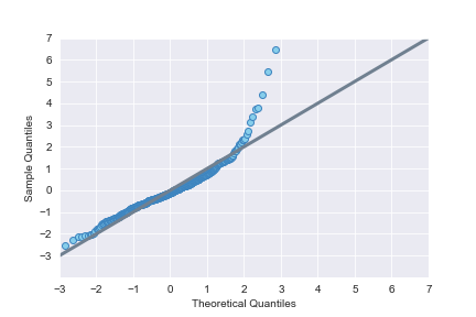
(a) Simple returns

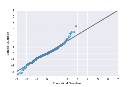
(b) Log returns

Figure 1: Quantile-Quantile plots for simple returns (a) and log returns (b). The returns are calculated as defined in section 2.

In order to ensure that we find the highest quality solutions, we run a calibration procedure that aims at finding the best values for $\lambda_{0}$ and $\lambda_{1}$ of both formulations separately. We run multiple QUBO instances as these parameters vary, repeat the procedure for each combination of QUBO formulation and solver and finally obtain that the following optimal values. A detailed explanation of our analysis is provided in the Appendix. The optimal values found are:

• $\lambda_{0}=1.2631$, $\lambda_{1}=300$ for the Sharpe Ratio Proxy formulation, solving with QBSolv

• $\lambda_{0}=1.2631$, $\lambda_{1}=300$ for the Sharpe Ratio Proxy formulation, solving with Hybrid

• $\lambda_{0}=0.7$, $\lambda_{1}=300$ for the Proposed Formulation, solving with QBSolv

• $\lambda_{0}=0.7$, $\lambda_{1}=300$ for the Proposed Formulation, solving with Hybrid

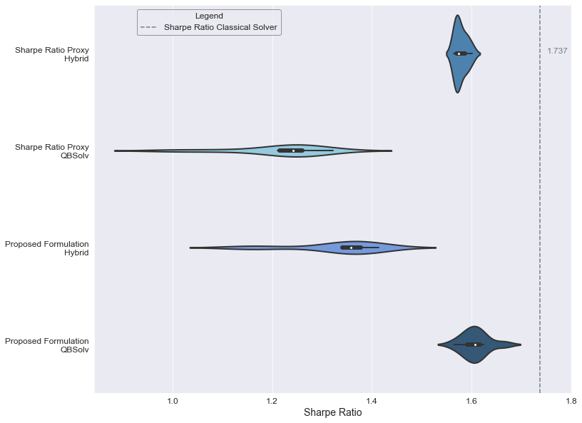
Figure 2: Violinplot of the results provided by each combination of QUBO formulation and solver. The statistics are drawn from $10$ feasible solutions with fixed values for the $\lambda$ coefficients. All solutions are feasible: for the Sharpe Ratio Proxy formulation, feasibility is given by the sum of asset weights equal to $1$, while for the Proposed Formulation we consider the constraint satisfied if $\mu^{T}y$ (ref. to Section 3.2) is in a neighbourhood of $1$, up to a factor equal to $2.5*10^{-4}$, which is given by multiplying the minimum discretization coefficient by the minimum expected return.

Then, having fixed the optimal values for $\lambda_{0}$ and $\lambda_{1}$, we retrieve $10$ more feasible solutions for each combination of QUBO formulation and solver, gathering stastistics of the results in terms of Sharpe Ratio values. In Figure 2 we compare the results with the solution found by the classical strategy implemented in the PyPortfolioOpt library pypfopt , which solves the problem as formulated in cornuejols_2006 . The Sharpe Ratio Proxy formulation and the Proposed Formulation lead to, respectively, $3888$ and $5184$ binary variables. The best results among the QUBO solutions are obtained by solving the Proposed Formulation with QBSolv. One noticeable factor is that for the two formulations, the best performances are reached by D-Wave Hybrid in one case and by QBSolv in the other. It can be argued that this effect is due to not only a different number of variables in the two formulations, for which the two solvers may behave differently, but also in the specific patterns of the QUBO matrices: given $432$ assets, the two discretization strategies yield a block size of $9$ variables representing each asset for the Sharpe Ratio Proxy formulation and a block size of $12$ variables for the Proposed Formulation. This constitutes a significant difference in the percentage size of the blocks which can drive different solvers to obtain different results. Finally, the gap between the classical and the best QUBO solutions can be arguably related to the capabilities of the solvers. Indeed, producing a thinner discretization would allow on one hand to represent quantities closer to the continuous values, while on the other hand it would lead to an increase in the number of variables, potentially causing solvers to generate poorer results.

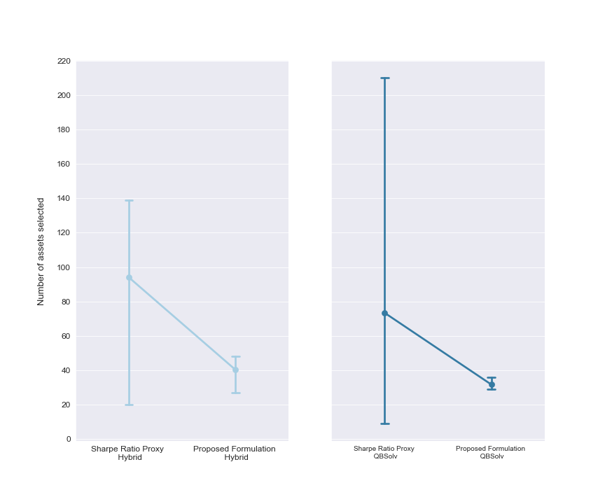
Figure 3: Minimum, maximum and mean (identified by the dot) in the number of assets selected over the 10 feasible solutions found. Left plot reports the statistics solving the two QUBO formulations using D-Wave Hybrid. Right plot, likewise, shows these results derived from the QBSolv solver.

Figure 3 shows statistics related to the number of assets selected using the two formulations and the different solvers. Having fixed the optimization strategy, the solutions show a two-fold result: the Proposed Formulation leads to a reduction in both the mean number of assets and reduces the variability. This behavior is found for each solver and can be arguably led back to the same previous remarks on the number of variables and block sizes differences in the two QUBO formulations.

5 Conclusions

The Portfolio Optimization problem is a well-known task in Financial Services and has recently drawn attention within the Quantum Computing literature thanks to the applicability of Quantum Annealers to solve the problem.

In this work we tackle a specific strategy to find the optimal allocation of investments over a set of assets, namely the Sharpe Ratio maximization. We extend a QUBO formulation proposed by venturelli , highlighting its benefits and potential drawbacks and propose a novel QUBO formulation to address the drawbacks. We run our experiments on classical and Quantum Computing hardware and compare our results both in terms of the QUBO formulation and in terms of the optimization solver.

Acknowledgments The authors wish to thank Domenico Fileppo, Marco Picardi, and Milena Stella, Intesa Sanpaolo S.p.A., for having supported this research work and Marco Magagnini, Data Reply S.r.l., for fruitful discussions.

Appendix 

Calibration Analysis

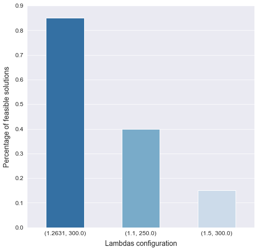
(a) Sharpe Ratio Proxy Hybrid

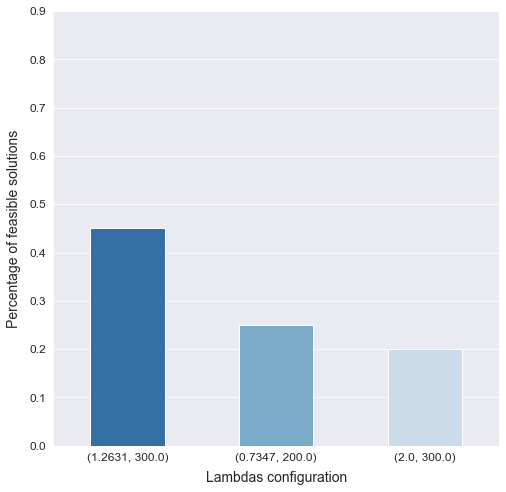
(b) Sharpe Ratio Proxy QBSolv

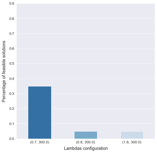
(c) Proposed Formulation Hybrid

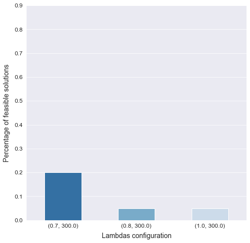
(d) Proposed Formulation QBSolv

Figure 4: Percentage of feasible solutions obtained from 20 runs for each lambda configuration, for each combination of formulation and solver.

We analyse in further details the calibration procedure that led to the choice of the optimal values for the coefficients $\lambda_{0}$ and $\lambda_{1}$ described in Section 4. In Figure 4 we show the results of our approach: for each combination of formulation and solver, we initially tested a grid of values for both coefficients; once the best lambda pairs were identified in terms of Sharpe Ratio value and corresponding constraint value, we performed 20 runs on each of these pairs and finally selected as optimal the one with the highest percentage of feasible solutions. Figure 4 reports multiple configurations of lambdas and the corresponding percentage number of feasible solutions. Configurations with lower $\lambda_{0}$ and higher $\lambda_{1}$ with respect to those represented here would, on one hand, lead to a higher percentage, while on the other decrease the value of Sharpe Ratio of the corresponding solutions. Therefore from Figure 4 stem the configurations that aim at maximizing the Sharpe Ratio, but also provide a number of feasible solutions as high as possible.

Multiple additional configurations have been tested, which however only led to infeasible solutions. Namely:

• Sharpe Ratio Proxy Hybrid:

  • $\lambda_{0}=2.4$ , $\lambda_{1}=200$

  • $\lambda_{0}=2$ , $\lambda_{1}=200$

  • $\lambda_{0}=2.4$ , $\lambda_{1}=300$

  • $\lambda_{0}=2.6$ , $\lambda_{1}=300$

• Sharpe Ratio Proxy QBSolv:

  • $\lambda_{0}=3.5$ , $\lambda_{1}=300$

  • $\lambda_{0}=2.6$ , $\lambda_{1}=300$

• Proposed Formulation Hybrid:

  • $\lambda_{0}=2.6$ , $\lambda_{1}=300$

• Proposed Formulation QBSolv:

  • $\lambda_{0}=50$ , $\lambda_{1}=500$

  • $\lambda_{0}=20$ , $\lambda_{1}=500$

  • $\lambda_{0}=20$ , $\lambda_{1}=700$

  • $\lambda_{0}=20$ , $\lambda_{1}=1000$

  • $\lambda_{0}=0.9474$ , $\lambda_{1}=300$

References

- \bibcommenthead
- (1) Markowitz, H.: PORTFOLIO SELECTION. https://doi.org/10.1111/j.1540-6261.1952.tb01525.x (1952)
- (2) Jorion, P.: Portfolio optimization in practice. Financial analysts journal 48(1), 68–74 (1992)
- (3) Maringer, D.: Heuristic optimization for portfolio management. Computational Intelligence Magazine, IEEE 3(4), 31–34 (2008). https://doi.org/10.1007/b136219
- (4) Cesarone, F., Scozzari, A., Tardella, F.: Efficient algorithms for mean-variance portfolio optimization with hard real-world constraints. G. Ist. Ital. Attuari 72 (2009)
- (5) Cesarone, F., Scozzari, A., Tardella, F.: Portfolio selection problems in practice: a comparison between linear and quadratic optimization models (2011)
- (6) Marzec, M.: Portfolio optimization: Applications in quantum computing. Handbook of high-frequency trading and modeling in finance, 73–106 (2016)
- (7) Kerenidis, I., Prakash, A., Szilágyi, D.: Quantum Algorithms for Portfolio Optimization (2019)
- (8) Lucas, A.: Ising formulations of many np problems. Frontiers in Physics 2 (2014). https://doi.org/10.3389/fphy.2014.00005
- (9) Rosenberg, G., Haghnegahdar, P., Goddard, P., Carr, P., Wu, K., De Prado, M.L.: Solving the optimal trading trajectory problem using a quantum annealer. In: Proceedings of the 8th Workshop on High Performance Computational Finance, pp. 1–7 (2015)
- (10) Phillipson, F., Bhatia, H.S.: Portfolio optimisation using the d-wave quantum annealer. In: International Conference on Computational Science, pp. 45–59 (2021). Springer
- (11) Morita, S., Nishimori, H.: Mathematical foundation of quantum annealing. Journal of Mathematical Physics 49 (2008). https://doi.org/10.1063/1.2995837
- (12) Incudini, M., Tarocco, F., Mengoni, R., Di Pierro, A., Mandarino, A.: Computing graph edit distance on quantum devices. Quantum Machine Intelligence 4(2), 1–21 (2022)
- (13) Kadowaki, T., Nishimori, H.: Quantum annealing in the transverse ising model. Physical Review E 58(5), 5355–5363 (1998). https://doi.org/10.1103/physreve.58.5355
- (14) Asproni, L., Caputo, D., Silva, B., Fazzi, G., Magagnini, M.: Accuracy and minor embedding in subqubo decomposition with fully connected large problems: a case study about the number partitioning problem. Quantum Machine Intelligence 2(1), 4 (2020). https://doi.org/10.1007/s42484-020-00014-w
- (15) Grant, E., Humble, T.S., Stump, B.: Benchmarking quantum annealing controls with portfolio optimization. Phys. Rev. Applied 15, 014012 (2021). https://doi.org/10.1103/PhysRevApplied.15.014012
- (16) Black, F., Litterman, R.B.: Asset allocation. The Journal of Fixed Income 1(2), 7–18 (1991). https://doi.org/10.3905/jfi.1991.408013
- (17) Kerenidis, I., Prakash, A., Szilágyi, D.: Quantum algorithms for portfolio optimization. In: Proceedings of the 1st ACM Conference on Advances in Financial Technologies, pp. 147–155 (2019)
- (18) Rebentrost, P., Lloyd, S.: Quantum computational finance: quantum algorithm for portfolio optimization. arXiv preprint arXiv:1811.03975 (2018)
- (19) Venturelli, D., Kondratyev, A.: Reverse quantum annealing approach to portfolio optimization problems. https://doi.org/10.1007/s42484-019-00001-w (2019)
- (20) Cornuejols, G., Tütüncü, R.: Optimization Methods in Finance. Mathematics, Finance and Risk, (2006). https://doi.org/10.1017/CBO9780511753886
- (21) PyPortfolioOpt library. https://pyportfolioopt.readthedocs.io/en/latest/