Magnetohydrodynamics with Physics Informed Neural Operators

Abstract

The modeling of multi-scale and multi-physics complex systems typically involves the use of scientific software that can optimally leverage extreme scale computing. Despite major developments in recent years, these simulations continue to be computationally intensive and time consuming. Here we explore the use of AI to accelerate the modeling of complex systems at a fraction of the computational cost of classical methods, and present the first application of physics informed neural operators to model 2D incompressible magnetohydrodynamics simulations. Our AI models incorporate tensor Fourier neural operators as their backbone, which we implemented with the TensorLY package. Our results indicate that physics informed neural operators can accurately capture the physics of magnetohydrodynamics simulations that describe laminar flows with Reynolds numbers $Re\leq 250$. We also explore the applicability of our AI surrogates for turbulent flows, and discuss a variety of methodologies that may be incorporated in future work to create AI models that provide a computationally efficient and high fidelity description of magnetohydrodynamics simulations for a broad range of Reynolds numbers. The scientific software developed in this project is released with this manuscript.

1 Introduction

Turbulence emerges from laminar flow due to instabilities, has many degrees of freedom, and is commonly found in fluids with low viscosity. Its time-dependent and stochastic nature make it an ideal sandbox to explore whether AI methodologies are capable of learning and describing nonlinear phenomena that manifests from small to large scales. While the Navier-Stokes equations may be used to study flows of non-conductive fluids, flows of ionized plasmas present in astrophysical phenomena may be considered perfectly conducting. These flows may be described by magnetohydrodynamics (MHD) equations, i.e., equations with currents, magnetic fields and the Lorentz force.

Theoretical and numerical modeling of MHD turbulence is critical to understand a variety of natural phenomena, encompassing astrophysical systems [1], plasma physics [2], and geophysics [3]. Some areas of interest in which MHD turbulence plays a crucial role are binary neutron star (BNS) mergers [4], black hole accretion, and supernova explosions [1]. The inherent complexity of MHD turbulence makes the modeling of these systems extremely difficult.

One of aspects of MHD turbulence responsible for such difficulty is the MHD dynamo, which amplifies the magnetic fields by converting kinetic energy into magnetic energy, starting at the smallest scales [5, 6, 1, 7]. In some cases, the MHD dynamo can produce amplification several orders of magnitude greater than that of the original fields [4, 1]. To resolve this magnetic field amplification, one must run simulations at the smallest of scales, where the MHD dynamo is most efficient [5]. This scale is set by the Reynolds number, $Re$, of the flow. The higher the $Re$, the smaller the scale of the most efficient MHD dynamo amplification. However, astrophysical simulations in particular are at such high Reynolds numbers that it would be unfeasible to fully resolve such turbulence [7]. Therefore, we must look to alternative ways to resolve such turbulent effects. One method is to approach MHD like a large eddy simulation (LES). In LES, one ensures they possess sufficient resolution to resolve the largest eddies and employs a subgrid-scale (SGS) models to resolve turbulence at smaller scales. Some recent works [8, 9, 10, 11, 12, 13, 14, 15, 16, 17, 18, 19] have adopted traditional LES style SGS models for MHD simulations. Other works [20, 21] have examined the use of deep learning models as the LES model in MHD simulations. These deep learning models can use data to learn MHD turbulence properties not present in the traditional LES models, but are still in their early stages of development.

Another approach consists of accelerating scientific software used to model multi-scale and multi-physics simulations with AI surrogates. Neural operators are a very promising class of deep learning models that can accurately describe complex simulations at a fraction of the time and computational cost of traditional large scale simulations [22, 22]. Recent studies have employed neural operators to model turbulence in hydrodynamic simulations [23, 24, 25]. In one study, the neural operators were compared to traditional LES style SGS models and were found to outperform the LES models in both accuracy and speed [25].

Physics informed neural operators (PINOs) incorporate physical and mathematical principles into the design, training and optimization of neural operators [26]. It has been reported in the literature that this approach accelerates the convergence and training of AI models, and in some cases enables zero-shot learning [27]. Several studies have illustrated the ability of PINOs to numerically solve partial differential equations (PDEs) that describe many complex problems [26, 27].

To further advance this line of research, in this paper we introduce AI surrogates to model multi-scale and multi-physics complex systems that are described by MHD equations. To this end, we produced 2D incompressible MHD simulations spanning a broad range of Reynolds numbers. We then trained PINOs with this data and evaluated them on a subset of simulations not observed in training. Specifically, we compared the PINO predictions and the simulation values as well as their kinetic and magnetic energy spectra. To the best of our knowledge, this is the first study seeking to reproduce entire MHD simulations with AI models. As such, we focused our efforts on finding the strengths and weaknesses of this approach rather than optimizing our models as much as possible. In doing so, this work provides a foundation of AI surrogates for MHD that future researchers will improve upon.

We organize this work as follows. In Section 2 we introduce the incompressible MHD equations, and describe the numerical methods used to generate MHD simulation data. Then, we describe PINOs, and how we used them to solve MHD equations in Section 3. Section 4 details the methods we followed to create our PINOs, including generation of random initial data, model architecture, training procedure, evaluation criteria, and a description of our computational resources. We present the results in Section 5. Final remarks and future directions of work are presented in Section 6.

2 Simulating Incompressible MHD

2.1 Equations

The goal of this work is to reproduce the incompressible MHD equations with PINOs. The incompressible MHD equations represent an incompressible fluid in the presence of a magnetic field $\mathbf{B}$. These equations are given by

$$\partial_{t}\mathbf{u}+\mathbf{u}\cdot\nabla\mathbf{u}=-\nabla\left(p+\frac{B^{2}}{2}\right)/\rho_{0}+\mathbf{B}\cdot\nabla\mathbf{B}+\nu\nabla^{2}\mathbf{u},$$ (1)

$$\partial_{t}\mathbf{B}+\mathbf{u}\cdot\nabla\mathbf{B}=\mathbf{B}\cdot\nabla\mathbf{u}+\eta\nabla^{2}\mathbf{B},$$ (2)

$$\nabla\cdot\mathbf{u}=0,$$ (3)

$$\nabla\cdot\mathbf{B}=0,$$ (4)

where $\mathbf{u}$ is the velocity field, $p$ is the pressure, $B$ is the magnitude of the magnetic field, $\rho_{0}=1$ is the density of the fluid, $\nu$ is the kinetic viscosity, and $\eta$ is the magnetic resistivity. We have two equations for evolution and two constraint equations.

To ensure the zero velocity divergence condition of Equation 3, the pressure is typically computed in such a way that this condition always holds true. This is generally done by solving a Poisson equation to calculate the pressure at each time step.

For the magnetic field divergence of Equation 4, we lack any additional free parameters to ensure that the equation holds true at all times. There are several ways to ensure that this condition holds including hyperbolic divergence cleaning [28] and constrained transport [29]. For this work, we decide to preserve the magnetic field’s zero divergence condition by instead evolving the magnetic vector potential $\mathbf{A}$. This quantity is defined such that

$$\mathbf{B}=\nabla\times\mathbf{A},$$ (5)

which ensures that the divergence of $\mathbf{B}$ is zero to numerical precision as the divergence of a curl of a vector field is zero. By evolving magnetic vector potential $\mathbf{A}$ instead of the magnetic field $\mathbf{B}$, we have a new evolution equation for the vector potential $\mathbf{A}$. This equation is given by

$$\partial_{t}\mathbf{A}+\mathbf{u}\cdot\nabla\mathbf{A}=\eta\nabla^{2}\mathbf{A}.$$ (6)

2.2 Numerical Methods

To simulate the MHD equations, we employed the Dedalus code [30], an open source parallelized spectral python package that is designed to solve general PDEs. To obtain interesting results without additional computational difficulty, we elected to solve the incompressible MHD equations in 2D with periodic boundary conditions (BCs). This results in us solving a total of 3 evolution PDEs at each timestep–2 for the velocity evolution and 1 for the magnetic vector potential evolution. To visualize and more easily diagnose problems with the simulations, we include an additional PDE to evolve tracer particles denoted by $s$. The tracer particles had an evolution equation given by

$$\partial_{t}s+\mathbf{u}\cdot\nabla s=\nu\nabla^{2}s.$$ (7)

Moreover, we employed a pressure gauge of $\int{p\,dx^{2}}=0$ for our equation. Numerically, most simulations were carried out on a unit length square grid at resolutions with a total number of grid points $N=128^{2}$, with $N_{x}=N_{y}=128$ points in the $x$ and $y$ directions, respectively. We also examined some lower resolution simulations with $N=64^{2}$ and higher resolution simulations with $N=256^{2}$ to explore how resolution may affect the results of the simulations.

As we have periodic BC, we employed a Fourier basis in each direction. To avoid aliasing error, we used a dealias factor of $3/2$ for these transformations. For timestepping, we used the RK4 integration method with a constant timestep of $\Delta t=0.001$. Simulation outputs were stored every 10 timesteps resulting in us recording data at interval $t=0.01$ time units. We ran these simulations until a time of $t=1$. For each set of parameters, we produced 1,000 simulations, each with different initial data.

2.3 Reynolds Number

An important consideration in this study was how the Reynolds number affects simulations and our AI model’s ability to reproduce the results of the simulations. The Reynolds number is a dimensionless quantity that expresses the ratio of inertial to viscous forces. The higher the Reynolds number is, the more prevalent the effects of small scale phenomena are to the simulation. This often gives rise to turbulence at high Reynolds numbers. For systems described by MHD equations, there are actually 2 types of Reynolds numbers of interest. They are the kinetic Reynolds number, $Re$, and the magnetic Reynolds number, $Re_{m}$. We define the quantities in our simulation such that these Reynolds numbers are given by

$$Re =1/\nu,$$ (8)

$$Re_{m} =1/\eta.$$ (9)

The ratio between these two Reynolds numbers is called the magnetic Prandtl number $Pr_{m}$ defined as

$$Pr_{m}=\frac{Re_{m}}{Re}=\frac{\nu}{\eta}.$$ (10)

In this study, we sought to characterize how the Reynolds number affects our models and determine if there is a cutoff Reynolds number, after which point, the models’ performance degrades considerably. We generally kept $Re=Re_{m}$ or, equivalently, $Pr_{m}=1$ unless otherwise noted and looked at Reynolds number values of 100, 250, 500, 750, 1,000, and 10,000.

One difference between MHD and hydrodynamic simulations is that, compared to the pure hydrodynamic case, much of the magnetic field energy is stored at high wavenumbers which occur at smaller scales. Thus, the models must be able to characterize high frequency features if they are to successfully reproduce the results of the magnetic field evolution.

3 Modeling MHD with PINOs

3.1 PINOs

The goal of a neural operator (NO) is to reproduce the results of an operator given some input fields using neural networks. A common class of operator often studied by NOs are PDEs. To model PDEs, NO take the coordinates, initial conditions (ICs), BCs, and coefficient fields as inputs. As outputs, NOs provide the solution of the operator, in this case the PDE, at the desired spacetime coordinates.

There are a variety of different NOs that have been studied in recent works. These include DeepONets, physics informed DeepONets, low-rank neural operators (LNO), graph neural operators (GNO), multipole graph neural operators (MGNO), Fourier neural operators (FNO), factorized Fourier neural operators (fFNO), and PINO [31, 32, 33, 34, 35, 22, 36, 26, 27]. In this study we use PINOs.

PINOs are a generic class of NOs that involve using an existing neural operator and employing physics informed methods in the training [26, 27]. Physics informed deep learning methods involves encoding known information about the physical system into the model during training [37, 38, 39, 40, 41, 42]. This physics information may include governing PDEs, symmetries, constraint laws, ICs, and BCs. By including such physical knowledge, physics informed methods enable better generalization of the results of deep learning models [42]. In systems where we have a lot of knowledge about the physical system like PDEs, such methods are especially useful as theoretically we could learn from just this physics knowledge. In practice, we add data to help PINOs converge to the correct solution more quickly.

One of the most common ways of encoding this physics into a neural network model is to incorporate physics information into the loss function [37, 38, 39, 40]. In other words, violations of these physics laws appear as terms in the loss function that are reduced over time during training. Thus, this technique treats physics laws as soft constraints learned by the neural network as it trains.

For the backbone NO, we selected a variant of fFNO [36] that employed the TensorLY [43] package to perform tensor factorization. We call this model a tensor Fourier neural operator (tFNO). The base FNO model [35] applies the fast Fourier transform (FFT) to the data to separate it into its component frequencies and apply its weights before performing an inverse FFT to convert back to real space. One particular feature of the FNO is its ability to perform zero-shot super-resolution, in which the model predicts on higher resolution data than it was trained on [35, 22]. We hope such properties of the FNO model would allow it to learn the high frequency properties of the MHD equations.

To further augment the model, we utilized factorization with TensorLY within the spectral layers of the model, so that it becomes an tFNO. The factorization was found to significantly improve the generalization of the neural network in the initial tests. The decision to use TensorLY was inspired by experimental code found in the GitHub repository of [26]. We will describe the model architecture in more detail in Section 4.2.

3.2 Applying to MHD Equations

Now let us discuss in more detail how to apply physics informed methods to model the MHD equations with neural operators. There are several aspects to modeling the MHD equations with such methods as denoted by each loss term. These are the data loss $\mathcal{L}_{\textrm{data}}$, the PDE loss $\mathcal{L}_{\textrm{PDE}}$, the constraint loss $\mathcal{L}_{\textrm{constr}}$, the IC loss $\mathcal{L}_{\textrm{IC}}$, and the BC loss $\mathcal{L}_{\textrm{BC}}$.

The data loss is modeled by obtaining simulation data and ensuring that the PINO output matches the simulation results. This requires us to produce a large quantity of simulations to provide sufficient training data like those described in Section 2.2 to span the solution space. We will discuss in more detail how we produced a sufficient number of simulations in Section 4.1. Then we use the relative mean squared error (MSE) between the simulation and the PINO predictions to define the value of the data loss $\mathcal{L}_{\textrm{data}}$.

The PDE loss describes the violations of the time evolution PDEs of the PINO outputs. Specifically, we encode these time evolution PDEs as part of the loss function. This requires us to represent the spatial and temporal derivatives of the output fields. Although some NOs are able to employ the automatic differentiation of the deep learning framework to calculate such derivatives [32], this method is too memory intensive for the tFNO architecture. Instead, we employ Fourier differentiation to represent the spacial derivatives, which computes highly accurate derivative values while conveniently assuming periodic BC that exists in our problem. For time derivatives, we use second order finite differencing. We note that such a time differencing technique cannot be used during the original simulation as this requires knowledge of future times to compute the time derivative of the current time.

Specifically, the PDEs we modeled with this technique were Equation 1 for velocity evolution and Equation 5 for magnetic potential evolution. In this case, the model has a total of 3 output fields in 2D, the velocity in the $x$ direction $u$, the velocity in the $y$ direction $v$, and the magnetic potential $A$. We also tested replacing the magnetic vector potential evolution with the magnetic field evolution of Equation 2, which results in 4 output fields in 2D. The fields in this case are the velocity in the $x$ direction $u$, the velocity in the $y$ direction $v$, the magnetic field in the $x$ direction $B_{x}$, and the magnetic field in the $y$ direction $B_{y}$. We note that in testing, the former representation of the MHD equations produced better results. The PDE loss $\mathcal{L}_{\textrm{PDE}}$ is then defined as the MSE loss between zero and the PDE, after putting all the terms on the same side of the equation.

Due to the complexity of both representations of the MHD equations, we tested the PDE loss on the data produced by the simulations. We found that the loss was small, albeit nonzero. This nonzero PDE loss was expected since the numerical methods for computing the derivatives during the simulation differs from those of computing the derivatives of the PDE during the loss function. Some particular notable differences are having fewer time steps in the output data than was used during the simulation, using different time derivative methods (e.g., RK4 during simulation vs second order finite differencing during the loss computation), and lacking dealiasing in the spatial derivatives in the PDE loss function.

The constraint loss illustrates the deviations of the elliptic constraint equations of the MHD equations. Specifically, these refer to the velocity divergence free condition of Equation 3 and the magnetic divergence free condition of Equation 4. We implemented these constraints similarly to the time evolution equations in the PDE loss, but without any time derivative terms. The constraint loss $\mathcal{L}_{\textrm{constr}}$ is then the MSE between each of the constraint equations and zero. We note that we are representing the magnetic fields by the magnetic potential, the magnetic field divergence free condition is satisfied up to the numerical precision of the curl operator regardless of the prediction of the neural network. However, we still include the term for completeness and this condition is not guaranteed to be nonzero if we are trying to compute the magnetic fields directly.

The IC loss tells the model to associate the input field with the output at $t=0$. Although this function can often be achieved with the data loss alone, the IC loss emphasizes the importance of predicting the correct IC and enables training in the absence of data. Both the significance of the IC and the ability to train without data stem from the PDE loss term. Theoretically, one can train by correctly predicting the IC, the BCs, and evolving the PDE correctly forward in time, although in practice, data helps the model converge more quickly. However, an incorrect IC results in the PDE evolving the wrong data forward in time. Thus, we add in the IC as its own term to encourage the model to first compute the IC correctly before learning the time evolution later in training. We calculate the IC loss $\mathcal{L}_{\textrm{IC}}$ by taking the input fields and computing the relative MSE between said input fields and the outputs fields at $t=0$.

Finally, the BC loss $\mathcal{L}_{\textrm{BC}}$ describes the violations of the boundary terms. In our case, the tFNO model architecture ensures that we have the desired periodic BC. Therefore, we do not use such a term in our model. However, we mention this term for generality because not all BCs and the periodicity of the tFNO architecture can be removed by zero padding the inputs along the desired non-periodic axis.

In physics informed deep learning methods, one must be careful when combining fields of different magnitudes to ensure they all have an equal contribution to the loss. Therefore, our model has the ability to normalize the input fields and denormalize the output fields by multiplying by predetermined constants. Moreover, we assign a weight to each term when combining loss terms for different fields and equation. We add additional weights when combining different losses. Thus, our loss $\mathcal{L}$ is given as

$$\mathcal{L} =w_{\textrm{data}}\mathcal{L}_{\textrm{data}}+w_{\textrm{PDE}}\mathcal{L}_{\textrm{PDE}}+w_{\textrm{constr}}\mathcal{L}_{\textrm{constr}}+w_{\textrm{IC}}\mathcal{L}_{\textrm{IC}}\,,$$ (11)

where $w_{\textrm{data}}$ is the data weight, $w_{\textrm{PDE}}$ is the PDE weight, $w_{\textrm{constr}}$ is the constraint weight, and $w_{\textrm{IC}}$ is the IC weight.

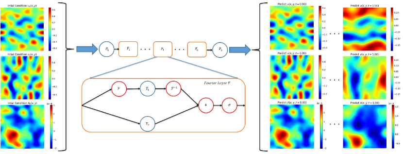
Figure 1: Architecture: Schematic representation of the architecture of our PINO models, which use the TensorLY [43] package to perform tensor factorization, thereby using tensor Fourier neural operators (tFNO) as the backbone of our AI models. On the far left, we display sample input fields that are fed into our PINO, which are composed of the $u$, $v$, and $A$ initial conditions (ICs). To the right of the input fields, we illustrate how the data is transformed as it goes through the model. First, this input data is lifted into a higher dimension representation by the neural network, $P_{1}$. Then, the data enters a series of Fourier layers labeled $\{F_{1},...,F_{i},...,F_{n}\}$. The inset zooms into one of these Fourier layers. In the inset, labelled as ”Fourier Layer F”, we apply a series of operations that consist of non-local integral operators and nonlinear activation functions. Specifically, $T_{1}$ represents a linear transform that employs CP decomposed tensors as weights, $T_{2}$ represents a local linear transform, and $\sigma$ represents a nonlinear activation function. $\mathcal{F}$ and $\mathcal{F}^{-1}$ stand for Fourier transform and inverse Fourier transform, respectively. Eventually, the neural network $P_{2}$ projects back into position space, producing the output shown on the right panels, which describe the time evolution of the system. These outputs are presented on the right of the image for the output fields $u$, $v$, and $A$ at times that range from $t=0$ to $t=1$.

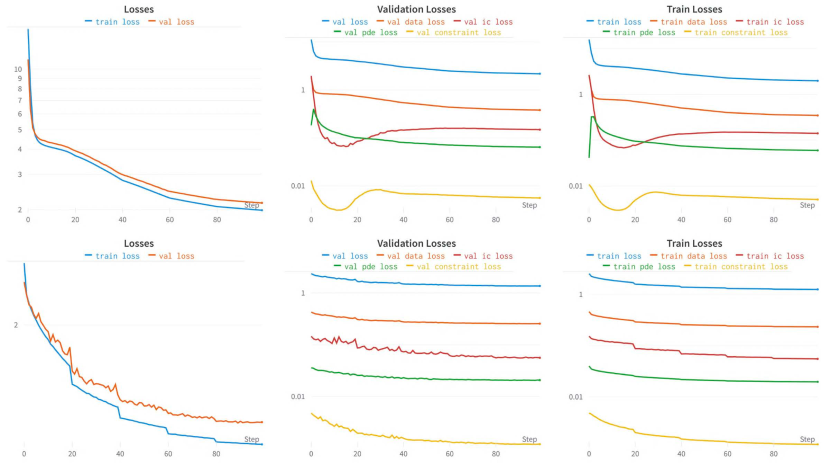
Figure 2: Loss Curves: Here we display the loss curves for the training. The top row depicts the original $Re=100$ case that was trained from scratch. The final checkpoint that was created by this run was used as the starting point for all models presented in this study. The bottom row shows an $Re=250$ model that was trained starting at said checkpoint The left panels depicts the total loss for the training and validation data on a linear scale. The center panels shows the training losses for each of the different types of losses we track–total loss, data loss, PDE loss, IC loss, and constraint loss. The right panels display these same losses, but for the validation data. To illustrate the different scales of these losses, the center and right panels use a log scale for the y-axis. The decreases in loss every 20 epochs occur due to the scheduler decreasing the learning rate by a factor of 2 at those epochs.

4 Methods

4.1 Data Generation

To generate the training data, we first needed to produce initial data before running it in the simulations described in Section 2.2. These initial data fields are produced using Gaussian random field (GRF) method similar to [27], in which the kernel was transformed into Fourier space to obey our desired periodic BCs. Specifically, we used the radial basis function kernel (RBF) to produce smooth initial fields. This kernel $k_{l}$ is defined as

$$k_{l}\left(x_{1},x_{2}\right)=\exp\left(-\frac{\left\|x_{1}-x_{2}\right\|^{2}}{2l^{2}}\right),$$ (12)

where $l$ is the length scale of typical spatial deviations in the data. We used $l=0.1$ for all fields in this works unless otherwise stated. We also needed to ensure that the velocity and magnetic fields are both divergence free. Therefore, we produced 2 initial data fields, the vorticity potential, $\psi$, and the magnetic potential $A$. We defined $\psi$ such that

$$\mathbf{v}=\nabla\times\psi,$$ (13)

which guarantees the velocity fields are divergence free initially. The magnetic potential $A$ is defined in Equation 6 in a similar manner to prevent the presence of divergences in the initial magnetic fields.

We multiplied the resulting initial data fields by a constant to ensure that the resulting fields have appropriate magnitude and are numerically stable. For example, we need to prevent Courant-Friedrichs-Lewy (CFL) condition violations, which can occur if the velocities are too high for a given resolution and timestep choice [44]. Numerical instabilities can also occur if the initial magnetic potential values are too high and may cause the simulation to fail. We chose these constants to be $c_{\psi}=0.1$ for the vorticity potential $\psi$ and $c_{A}=0.005$ for the magnetic potential $A$.

4.2 Model Architecture

A schematic of the tFNO models utilized in this study is presented in Figure 1. The size and dimensions of the model can be described by 3 hyperparameters–the width, the number of Fourier modes, and the number of layers. We used 4 layers for all models in this work. The width and number of Fourier modes were the same across all layers of the model in this work and were both set to 8 unless stated otherwise. Although we suspect that we could get better results by increasing the these hyperparameters, especially the number of Fourier modes which may have helped the models reproduce small scale features in the flow, doing so proved too memory intensive for our GPUs.

We factorized the weight tensors within the spectral layers with TensorLY to improve generalizability. Specifically, we used a canonical polyadic tensor decomposition [45] with a rank of 0.5 to perform this factorization. Prior to producing the outputs, the models employ a fully connected layer of width 128.

In addition, the model normalizes its data internally by dividing by a constant input normalization factor to ensure that magnitude varying inputs are treated the same way. In particular, the magnitude of the magnetic potential $A$ was considerably less than that of the velocity fields $u$ and $v$. Similarly, we multiplied the output by a constant output normalization factor to alleviate the tFNO model from having to produce results with significantly different magnitudes. For this work, we used the same value for the input and output normalization fields of $1$ for the velocity fields and $0.00025$ for the magnetic potential $A$. Finally, we selected the Gaussian error linear unit (GELU) for the nonlinearity of these models [46].

4.3 Training

To accelerate the training, we would employ transfer learning across different Reynolds number $Re$. Specifically, we began by training a model at a resolution $N=128^{2}$ at $Re=100$ from scratch. The checkpoint generated from this run was used as the starting point for all the other models. In turn, this transfer learning saved considerable time when training new models. We trained models initialized from the aforementioned checkpoint at resolution of $N=128^{2}$ for $Re$ values of $Re=\{100,250,500,750,1000,10000\}$. We then compared these models to additional ones trained at resolutions of $N=64^{2}$ and $N=256^{2}$. These models were for the same $Re$ as the previous $N=128^{2}$ resolutions, except for $Re=10,000$. All models trained using $950$ simulations that encompassed the training data and were evaluated using the remaining $50$ simulations that served as the test data. In Figure 2, we display some loss curves for the $Re=100$ model that was trained from scratch and for the $Re=250$ model both at resolutions of $N=128^{2}$.

For most models, we trained on all available timesteps. However, we wanted to see the effect of being asked to output fewer time steps had on the model. Therefore, we trained additional models that skipped several timesteps. These trained at $Re=250$ and $N=128^{2}$ and are described further in Section 5.

We trained these models using the PyTorch deep learning framework [47]. All models in this study trained for 100 epochs starting from the pretrained checkpoint. Most models used an initial learning rate of $5\times 10^{-4}$. However, the models at $N=128^{2}$ with $Re$ values of $750$, $1,000$, and $10,000$ had initial learning weights of 0.001. The different initial learning rate for these runs was unintentional. We suspect this higher may have improved the performance of these runs based on how they perform compared to the same $Re$ runs at other resolutions, but no rigorous study of learning rate optimization was performed. We employed a scheduler to decrease the learning rate by a factor of 2 every 20 epoch to help finetune the models. We selected an AdamW optimizer [48] to optimize the models. This optimizer had a weight decay value of 0.1, $\beta_{1}=0.9$, $\beta_{2}=0.999$.

We set most of the weight hyperparameters of the various loss terms to $1$ with a few notable exceptions. We set the weight of the magnetic potential evolution equation loss $w_{\textrm{DA}}$ to $10^{6}$ as the magnitude of the term was small compared to that of the other evolution equations. In addition, we used a value of the constraint loss weight $w_{\textrm{constr}}$ of $10$. Finally, we selected $w_{\textrm{data}}=5$ as our data loss weight. We logged specific hyperparameters used in training each PINO using WandB [49] for reproducibility. In addition, we ran an experiments where we modified the PDE loss weight $w_{\textrm{PDE}}$ hyperparameter to explore its impact on our AI models. These were done at $Re=250$ and $Re=500$ both at $N=128^{2}$ and are described further in Section 5.

4.4 Computational Resources

We initially computed a subset of the results on the Pittsburgh Supercomputing Center’s Bridges-2 cluster. Specifically, we used the V100 GPUs on this cluster. We primarily used the 16 GB variant of these GPUs, though some cases utilized the 32 GB variation. To generate the training data, for the initial portion of the study, we utilized the CPUs on the Bridges-2 cluster’s GPU nodes. We used a single GPU node for this process, which has two Intel Xeon Gold 6248 “Cascade Lake” CPUs, which have 20 cores, 2.50-3.90GHz, 27.5 MB LLC, 6 memory channels each. After verifying that our models worked as expected, we scaled up our experiments using NCSA’s Delta cluster. For training, we employed the cluster’s NVIDIA A100 GPUs, training each model on a single GPU. To generate an expanded quantity of training data, we employed the Delta cluster’s CPU nodes. These come equipped with 128 AMD EPYC 7763 “Milan” (PCIe Gen4) CPUs. We parallelized the generation of the training data such that multiple simulations were generated at one, but each only using one core. We considered low ($N=64^{2})$, standard ($N=128^{2})$, and high resolution ($N=256^{2})$ simulations.

4.5 Evaluation Criteria

To evaluate the performance of our PINO models, we look at the relative MSE. This allows us to compare errors of the various fields despite them differing in magnitude. We report the relative MSE for the predictions the PINOs on the test dataset for each field of interest. In addition, we compute the total relative MSE, $\textrm{MSE}_{tot}$, for our PINOs on this data which we defined as

$$\textrm{MSE}_{tot}=\textrm{MSE}_{u}+\textrm{MSE}_{v}+\textrm{MSE}_{A},$$ (14)

where $\textrm{MSE}_{u}$, $\textrm{MSE}_{v}$, and $\textrm{MSE}_{A}$ are the MSE values of the $u$, $v$, and $A$ fields respectively. In addition, we computed the kinetic energy spectra $E_{kin}(k)$ and magnetic energy spectra, $E_{mag}(k)$, of the PINO predictions and the ground truth simulations. This allowed us to compare how the models perform at various scales as specified by the wavenumber $k$.

Table 1: Summary of Results: The $Re$ column displays the Reynolds number of the model. The Resolution column provides the resolution of the model. The $N_{train}$ and $N_{test}$ columns tell us how many simulations were used in training and testing respectively for each PINO. The MSE $u$, MSE $v$, and MSE $A$ give us the relative MSE values of the $u$, $v$, and $A$ fields respectively. The far right column, MSE Total, lists the sum of the MSE values of the $u$, $v$, and $A$ fields.

• Standard Runs	$\mathbf{Re}$	Resolution	MSE u	MSE v	MSE A	MSE Total
  	100	$128^{2}$	0.019433	0.023787	0.039242	0.082462103
  	250	$128^{2}$	0.065276	0.070364	0.119925	0.255565267
  	500	$128^{2}$	0.136089	0.146443	0.262841	0.545372143
  	750	$128^{2}$	0.160067	0.168168	0.313788	0.642023818
  	1000	$128^{2}$	0.185853	0.19528	0.362628	0.7437606
  	10000	$128^{2}$	0.280736	0.28256	0.557567	1.120862162
  	100	$64^{2}$	0.018748	0.022466	0.03603	0.077244182
  	250	$64^{2}$	0.062604	0.070628	0.122528	0.255759554
  	500	$64^{2}$	0.129726	0.139503	0.249703	0.518932519
  	750	$64^{2}$	0.170337	0.180869	0.325797	0.67700303
  	1000	$64^{2}$	0.196846	0.207568	0.374421	0.778835213
  	100	$256^{2}$	0.019498	0.023901	0.037558	0.080957422
  	250	$256^{2}$	0.064941	0.076371	0.130074	0.271386759
  	500	$256^{2}$	0.134618	0.147628	0.261671	0.543917469
  	750	$256^{2}$	0.176292	0.190424	0.339657	0.706372823
  	1000	$256^{2}$	0.203172	0.218052	0.389165	0.81038871
  $\mathbf{w_{\textrm{PDE}}}$	$\mathbf{Re}$	Resolution	MSE u	MSE v	MSE A	MSE Total
  0	250	$128^{2}$	0.065495	0.070718	0.120027	0.256239378
  1	250	$128^{2}$	0.065276	0.070364	0.119925	0.255565267
  2	250	$128^{2}$	0.06514	0.070161	0.119934	0.25523497
  5	250	$128^{2}$	0.064882	0.069786	0.120038	0.254706307
  10	250	$128^{2}$	0.064688	0.069522	0.120324	0.254534433
  0	500	$128^{2}$	0.136623	0.147041	0.264064	0.547728002
  1	500	$128^{2}$	0.136089	0.146443	0.262841	0.545372143
  2	500	$128^{2}$	0.135796	0.146161	0.262429	0.544385653
  5	500	$128^{2}$	0.135441	0.14579	0.262019	0.543249941
  10	500	$128^{2}$	0.135667	0.145995	0.262715	0.544377502
  $\mathbf{t_{step}}$	$\mathbf{Re}$	Resolution	MSE u	MSE v	MSE A	MSE Total
  1	250	$128^{2}$	0.065276	0.070364	0.119925	0.255565267
  2	250	$128^{2}$	0.064159	0.069215	0.115976	0.249350436
  3	250	$128^{2}$	0.062734	0.067394	0.111937	0.242065011
  4	250	$128^{2}$	0.061139	0.065587	0.108474	0.235199714

5 Results

Here we present results for the accuracy with which our PINO models solve the MHD equations, and then compare these AI predictions with high performance computing MHD simulations. These simulations are evolved in the time domain $t\in[0,1]$. We present results for a broad range of Reynolds number $Re$, summarized in Table 1. Our PINO simulations and traditional MHD simulations are compared throughout their entire evolution, and then we take a snapshot of their evolution at $t=1$. We do this to capture the largest discrepancy between AI-driven simulations and traditional PDE solvers at a time where numerical errors and other discrepancies between these methodologies are maximized. We examined a variety of factors that impact the performance of our models, including:

• Reynolds number: We quantify the ability of our AI surrogates to describe the physics of MHD simulations for laminar and turbulent flows. In general, simulations with higher Reynolds numbers, $Re$, i.e., more turbulent flows, are more challenging to describe accurately.

• Resolution: We compare the performance of our models using three grid resolutions: $64^{2}$, $128^{2}$, and $256^{2}$, which we denote as the low, standard, and high resolutions, respectively. In what follows, we present results for the standard resolution, $N=128^{2}$. Results for low and high resolutions are presented in A.

• PDE loss weight: We looked at how changing the PDE loss weight $w_{\textrm{PDE}}$ impacts our AI models. This represents how much the physics informed aspect of the model improved the results. We tested $w_{\textrm{PDE}}$ values of 0, 1, 2, 5, and 10.

• Timestep: By default, our AI models use 101 timesteps to cover the time range $t\in[0,1]$. We use the quantity $t_{\textrm{step}}$ to represent the frequency of sampling from the full set of times. For example, $t_{\textrm{step}}=1$ uses all timesteps and $t_{\textrm{step}}=2$ uses every other timestep. For this experiment, we used $t_{\textrm{step}}$ values of 1, 2, 5, and 10.

5.1 Resolution

To begin with, in the left panel of Figure 3 we present how the data loss MSE varies with $Re$ for $N=128^{2}$. Therein we see the loss of each field $(u,v,A)$ as well as the total loss as a function of $Re$. We observe that the two velocity fields $u$ and $v$ possess around the same MSE value as one would expect. In contrast, the MSE for the magnetic potential field $A$ is larger than that of the velocity fields. Moreover, the MSE value of the $A$ field increases faster compared to those of the velocity fields $u$ and $v$. In the right panel of Figure 3 we see the total MSE as a function of $Re$ for three different resolutions, $N=\{64^{2},128^{2},256^{2}\}$. If we combine these two sets of results, we realize that our AI surrogates can produce reliable MHD simulations for $Re\leq 250$, and that the main factor that degrades the accuracy of our AI surrogates is the ability to capture detailed features of the vector potential $A$ in turbulent flows. We also notice that the resolution of the training data does not have a major impact in the accuracy of our AI surrogates.

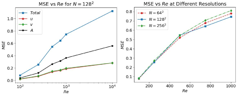
Figure 3: Left panel MSE vs Reynolds number $Re$ at a resolution of $N=128^{2}$. We include the total MSE and the MSE for each of the fields the model is trying to reconstruct–velocity in the $x$ direction $u$, the velocity in the $y$ direction $v$, and magnetic vector potential $A$. Right panel Total MSE vs Reynolds number $Re$ for grids of size $N=\{64^{2},128^{2},256^{2}\}$. We compare these resolutions for $Re=\{100,250,500,750,1000\}$.

5.2 PDE Weight

Figure 4 illustrates how the MSE changes with PDE weight, $w_{\textrm{PDE}}$, for $Re=250$ and $Re=500$. We observe that the MSE improves as we increase $w_{\textrm{PDE}}$. The only exception of $Re=500$ and $w_{\textrm{PDE}}=10$ which increases in MSE compared to $w_{\textrm{PDE}}=5$, but still less than the other $w_{\textrm{PDE}}$ values at $Re=500$. However, we should observe that while including violations of the PDE into the loss function improves the result, their contribution is only marginal.

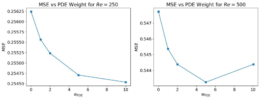
Figure 4: MSE vs PDE weight Impact of PDE weight, $w_{\textrm{PDE}}$, on the performance of AI surrogates in terms of total MSE for $Re=250$ (left panel). and $Re=500$ (right panel) simulations. We show results for $w_{\textrm{PDE}}$ values of $0$, $1$, $2$, $5$, and $10$.

5.3 Timesteps

Figure 5 illustrates, for the $Re=250$ model, how the total MSE varies with the number of timesteps, $t_{\textrm{step}}$. We observe that the fewer timesteps the model is required to output data for (higher $t_{step}$), the better the performance of the model—though this improvement is marginal.

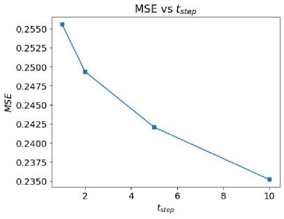
Figure 5: MSE vs Timestep Total MSE vs timestep, $t_{\textrm{step}}$, for values $t_{step}=\{1,2,5,10\}$.

5.4 Pair-wise comparison of traditional and AI-driven MHD simulations

We now compare traditional MHD simulations with predictions from AI surrogates assuming a grid of size $N=128^{2}$, and $t_{step}=1$. In Figure 6-11 we present snapshots of the systems’ evolution at time $t=1$ to show the largest discrepancy between ground truth values (traditional MHD simulations) and AI predictions. These results illustrate initial conditions, targets, prediction, and MSEs between target and AI predictions. At a glance, we observe that AI models appear to possess the ability to resolve large scale features, but struggle to resolve cases with small scale structure. This small scale structure arise at higher $Re$ and is observed most strongly in the $A$ field. We summarize below the main findings of these studies using Table 1, Figure 3 and Figures 6-11:

• $Re=100$. Figure 6 shows that PINO models provide an accurate description of these MHD simulations. Quantitatively and quantitatively PINOs can resolve the dynamics of the velocity field, $(u,v)$, and the vector potential, $A$. We also notice that the largest discrepancy between AI predictions and traditional MHD simulations at $t=1$ is $\leq 4\%$ for each of the fields.

• $Re=250$. Figure 7 shows that PINOs provide a reliable description of the dynamics of these simulations. The velocity field and vector potential potential are accurately described, with MSEs $\leq 7\%$ and $\leq 10\%$, respectively.

• $Re=500$. Figure 8 shows that PINOs capture well large scale features of these simulations. In particular, the velocity field can be recovered with MSE $\leq 14\%$. On the other hand, detailed features of the vector potential are not completely resolved, and the MSE is $\leq 26\%$.

• $Re=750$. Figure 9 shows that PINO MHD simulations can resolve large scale features of the velocity field, with MSE $\leq 16\%$, which is similar to simulations with $Re=500$. Similarly, large scale features of the vector potential are well described. However, as these systems become more turbulent, small scale features of the vector potential are not captured by PINOs, and report an increase in MSE, i.e., $\leq 31\%$.

• $Re=1,000$. Figure 10 presents a similar story to the two previous cases. Large scale structure is well described, and the MSE for the velocity field is $\leq 18\%$. However, it is difficult to capture the small scale features of the magnetic field, which now evolve in a rather complex manner for these turbulent systems.

• $Re=10,000$. Figure 11 indicates that, for very turbulent MHD systems, PINOs can only reproduce some of the large scale features of the flow, but struggle to reproduce many of the detailed features. One particular feature that the PINO misses is the small scale fluctuations in the velocity fields $u$ and $v$ that likely result from strong magnetic fields in those areas. In other words, the PINO cannnot resolve the effect of the magnetic field on the fluid motion. For the magnetic potential $A$, the PINO model appears to miss most of the important features at first glance. If we look more closely, we observe that the PINO appears, to some extent, to reproduce the mean field value over some very large regions. However, this comes at the cost of missing any sort of interesting details in the magnetic field.

In summary, Figures 6-11 show that our PINO models can successfully reproduce large scale features of MHD simulations, but had difficulty resolving detailed features for large Reynolds numbers, especially for the magnetic potential, which is known to store its energy at higher wavenumbers. Thus, in the following section we explored the ability of PINOs to learn the right data features associated to low and high wavenumbers as the simulation evolves in time.

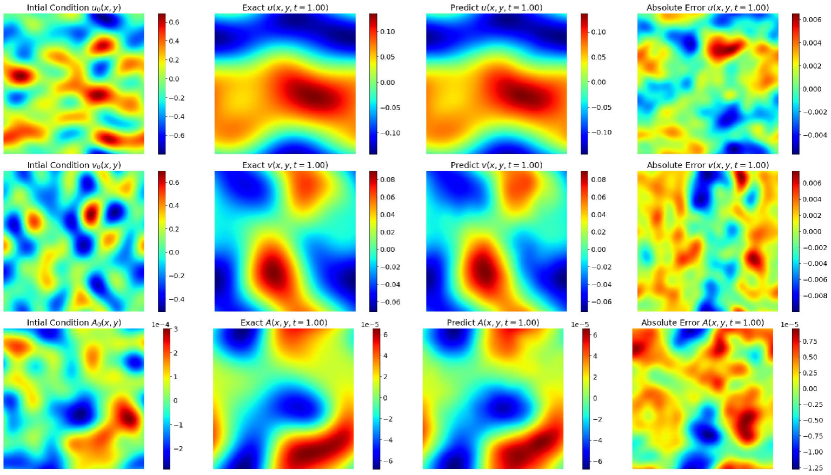
Figure 6: $\mathbf{Re=100}$ MHD Simulations Results of the PINO model on sample test data from the $Re=100$ simulations. The rows correspond to the fields of interest with the velocity in the x direction $u$, the velocity in the y direction $v$, and the magnetic potential $A$ being the quantities featured in the top, middle, bottom rows, respectively. The far left column depicts the initial condition given to the PINO model. The center left column shows the ground truth at time $t=1$. In the center right column, we present the PINO predictions at time $t=1$. The far right column error between the ground truth and the PINO predictions at $t=1$.

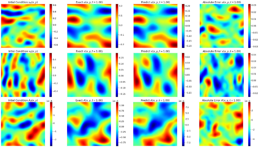
Figure 7: $\mathbf{Re=250}$ MHD Simulations Same as Figure 6 but now for a test set from the $Re=250$ simulations.

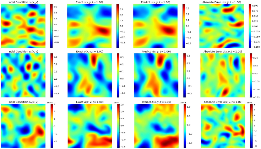
Figure 8: $\mathbf{Re=500}$ MHD Simulations Same as Figure 6 but now for a test set from the $Re=500$ simulations.

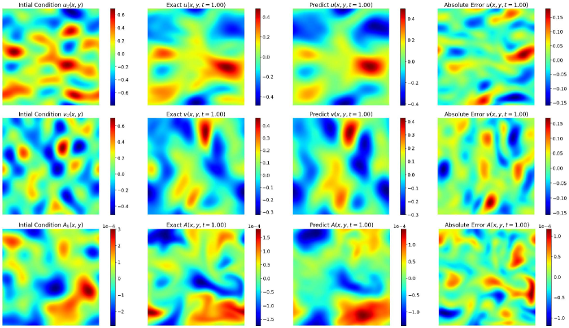
Figure 9: $\mathbf{Re=750}$ MHD Simulations Same as Figure 6 but now for a test set from the $Re=750$ simulations.

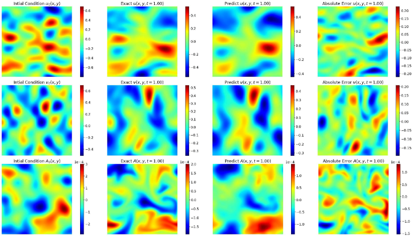
Figure 10: $\mathbf{Re=1,000}$ MHD Simulations Same as Figure 6 but now for a test set from the $Re=1,000$ simulations.

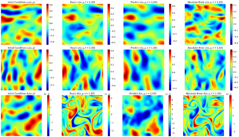
Figure 11: $\mathbf{Re=10,000}$ MHD Simulations Same as Figure 6 but now for a test set from the $Re=10,000$ simulations.

5.5 Spectra Results

We analyzed the magnetic and kinetic energy spectra of the simulations in Figure 12. Therein we observe that for both the kinetic and magnetic energy spectra, the PINO models performed well at low wavenumbers $k$. However, the PINOs were not able to accurately reproduce the energy spectra at high wavenumbers. Interestingly, at low $Re$, the PINOs tended to overshoot the ground truth energies at high wavenumbers. While at high $Re$, the PINOs tended to undershoot the ground truth energies at high wavenumbers.

Moreover, large Reynolds number simulations usually store more energy at higher wavenumbers. This is especially true for the magnetic energy, which tends to peak at later wavenumbers in higher $Re$ simulations. Therefore, the spectra plots in Figure 12 indicate that the difficulties the PINOs had in reproducing the simulations at high $Re$ and the magnetic potential field $A$ may stem from their relatively poor performance at high wavenumbers. Therefore, future work should focus on developing methods that enable PINOs to capture data features contained at high wavenumbers.

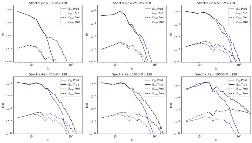
Figure 12: Spectra The panels show the kinetic and magnetic spectra for each PINO model and simulation at time $t=1$. We present the kinetic energy spectra as solid lines and the magnetic energy spectra as dashed lines. The ground truth simulations are illustrated in black while the PINO predictions are in blue. The top row presents from left to right the $Re=100$, $Re=250$, and $Re=500$. The bottom row contains the $Re=750$, $Re=1,000$, and $Re=10,000$ cases.

6 Conclusions

In this work we presented the first application of PINOs to produce 2D incompressible MHD simulations for a variety of initial conditions and Reynolds numbers. We demonstrated how to incorporate physics principles, and suitable gauge conditions, for the training and optimization of our AI surrogates. Once fully trained, we found that our PINO models were able to accurately describe MHD simulations with Reynolds numbers $Re\leq 250$ throughout the entire evolution of the system, i.e., $t\in[0,1]$. For other systems with larger Reynolds numbers, we found that PINOs provide a reliable description of the system at earlier times, but as the system evolves, PINO simulations gradually degrade in accuracy. We first noticed this behaviour in the evolution of the magnetic potential, $A$, which we used to evolve the magnetic fields, for MHD simulations with $Re>500$. We explored this issue in detail, and found that this issue may likely stem from the PINOs’ difficulty in learning physics contained at high wavenumbers.

We suggest that future work should focus on optimizing neural operators at these high wavenumbers. One suggestion would be to increase the number of Fourier modes used by our tFNO backend. We were memory limited and were restricted to 8 Fourier modes to store the model in GPU memory. Recent work involving FNOs for hydrodynamic turbulence modeling have had success with using 20 Fourier modes [25]. One should be cautious, however, since using too many Fourier modes may also introduce numerical noise and complicate the resolution of small scale features in the data. We also suggest to use emergent methods to train PINOs using high resolution datasets which, while difficult to fit in a state-of-the-art GPU, may be readily used in AI-accelerator machines, as those housed in multiple supercomputing centers in the US and elsewhere, e.g., the Argonne Leadership Computing Facility AI-Testbed.

Another suggestion is to develop methods that enable PINOs to learn the turbulence statistics of the MHD simulation in addition to the flow. For example, one could incorporate the kinetic and magnetic energy spectra into the loss function and weigh in the contribution of the high wavenumber portions of the spectrum appropriately. Through this approach, PINOs may may predict the flow with the correct turbulent characteristics even if they are unable to accurately model the details of the flow. It is also advisable to go beyond the use of physics-informed loss functions, which only provide static optimization at present. A more suitable approach for these types of complex systems would entail coupling physics-informed loss functions with online or reinforcement learning that dynamically steer the AI surrogate to the right answer during the optimization procedure as new data features, such as magnetic fields, arise in the simulation data. We expect that the work we have presented here, in terms of data generators, AI surrogates, and optimization approaches for complex systems, may provide a stepping stone to other AI practitioners who are developing novel methods to model complex systems, such as turbulent MHD simulations.

References

Appendix A Additional results for low and high resolution simulations

Here we provide additional results that further establish the results we discussed in the main body of the article. In summary, Figures 13-22 show that using low, standard or high resolution simulations have a marginal impact in the performance of PINOs to capture the dynamics of turbulent MHD systems. What we learn from these studies is that what really matters is that PINOs are able to dynamically assign the correct kinetic and magnetic energy at high wavenumbers as the system evolves in time. The current approach in which physics-inspired loss functions remain static should be replaced by dynamic loss functions. This approach will be explored in the future.

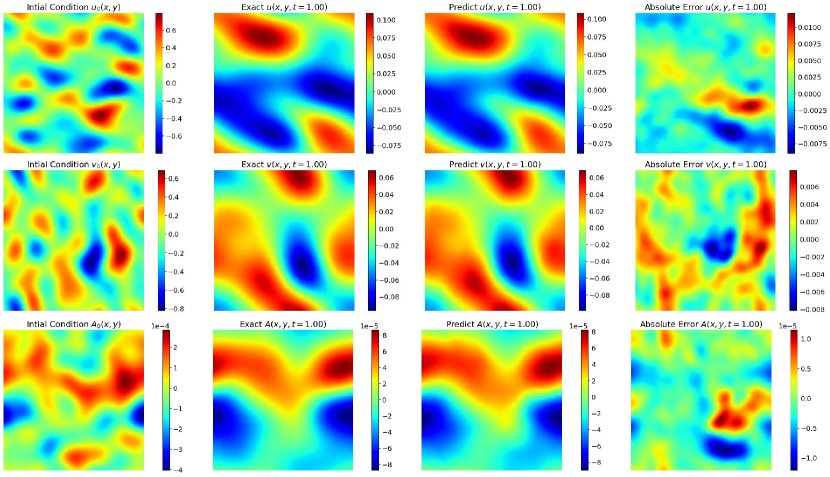
Figure 13: $\mathbf{Re=100}$ MHD Simulations As Figure 6 but now for a test set with resolution of $N=64^{2}$ grid points.

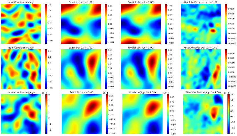
Figure 14: $\mathbf{Re=100}$ MHD Simulations As Figure 13 but now for a test set with resolution of $N=256^{2}$ grid points.

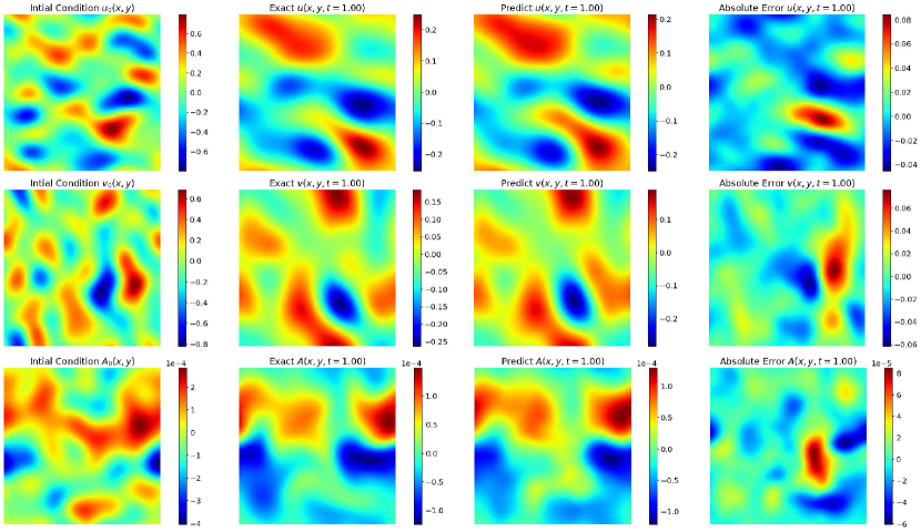
Figure 15: $\mathbf{Re=250}$ MHD Simulations As Figure 13 but now for a test set from the $Re=250$ simulations with resolution of $N=64^{2}$ grid points.

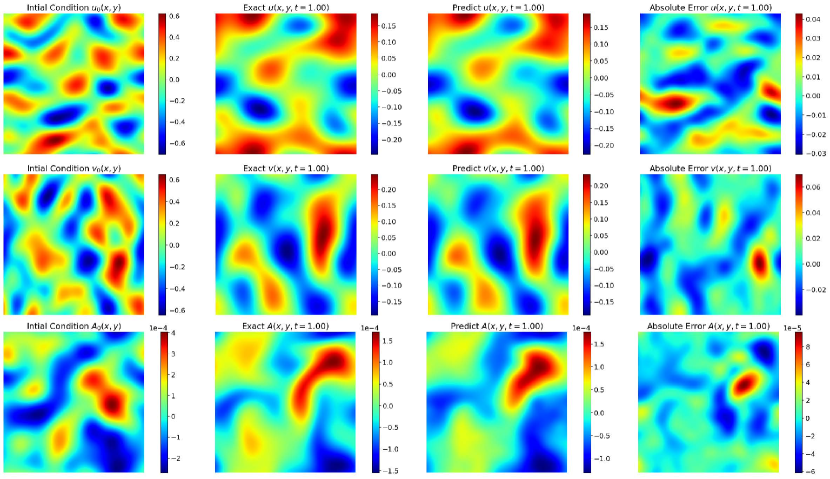
Figure 16: $\mathbf{Re=250}$ MHD Simulations Same as Figure 15 but now for a test set with resolution of $N=256^{2}$ grid points.

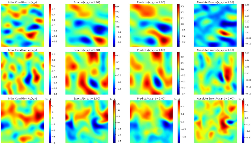
Figure 17: $\mathbf{Re=500}$ MHD Simulations As Figure 13 but now for a test set from the $Re=500$ simulations with resolution of $N=64^{2}$ grid points.

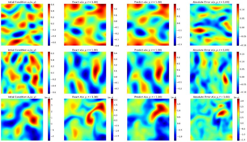
Figure 18: $\mathbf{Re=500}$ MHD Simulations Same as Figure 17 but now for a test set with resolution of $N=256^{2}$ grid points.

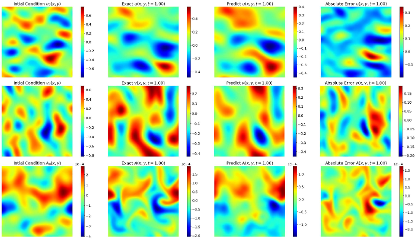
Figure 19: $\mathbf{Re=750}$ MHD Simulations As Figure 13 but now for a test set from the $Re=750$ simulations with resolution of $N=64^{2}$ grid points.

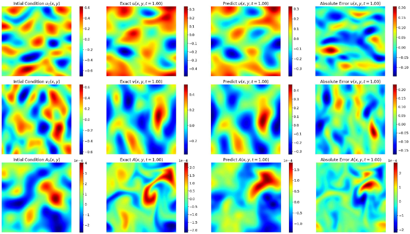
Figure 20: $\mathbf{Re=750}$ MHD Simulations Same as Figure 19 but now for a test set with resolution of $N=256^{2}$ grid points.

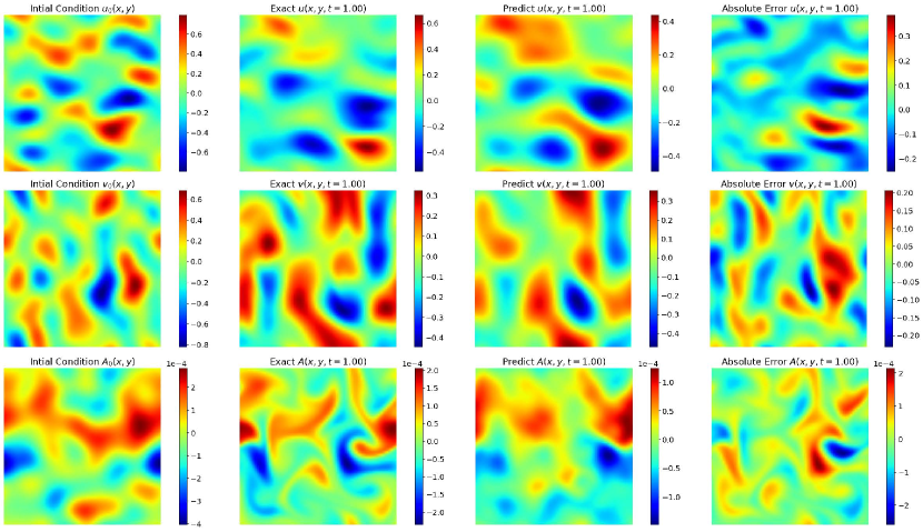
Figure 21: $\mathbf{Re=1,000}$ MHD Simulations As Figure 13 but now for a test set from the $Re=1,000$ simulations with resolution of $N=64^{2}$ grid points.

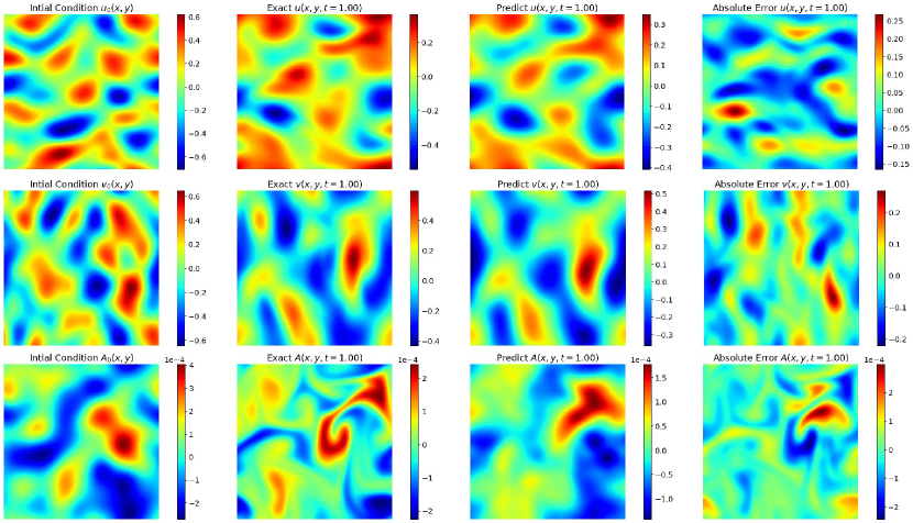
Figure 22: $\mathbf{Re=1,000}$ MHD Simulations Same as Figure 21 but now for a test set with resolution of $N=256^{2}$ grid points.

Appendix B Additional results for low and high resolution spectra

Figures 23 and 24 show that low and high resolution MHD simulations have similar properties in their distribution of kinetic and magnetic energy at different wavenumbers. Thus, using high resolution data to train PINOs does not constitute a silver bullet to ensure that PINOs capture the small scale structure of turbulent flows, in particular that related to the impact of magnetic fields in the evolution of these systems.

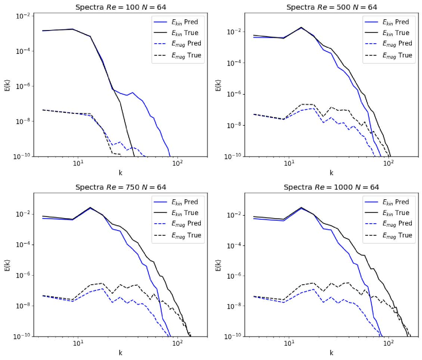
Figure 23: Spectra at Different Resolutions Same as Figure 12 for the remaining $N=64^{2}$ models with $Re$ not plotted elsewhere.

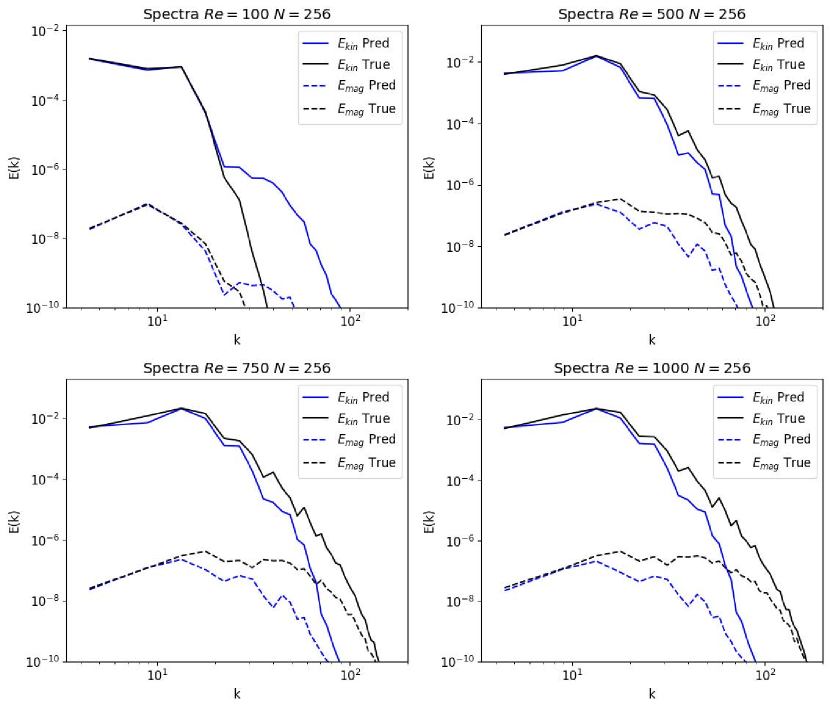
Figure 24: Spectra at Different Resolutions Same as Figure 12 for the remaining $N=256^{2}$ models with $Re$ not plotted elsewhere.

References

- [1] Beresnyak A 2019 Living Reviews in Computational Astrophysics 5 2 ISSN 2365-0524 URL https://doi.org/10.1007/s41115-019-0005-8
- [2] Schekochihin A A 2022 Journal of Plasma Physics 88 155880501
- [3] Pouquet A, Rosenberg D, Stawarz J and Marino R 2019 Earth and Space Science 6 351–369 (Preprint https://agupubs.onlinelibrary.wiley.com/doi/pdf/10.1029/2018EA000432) URL https://agupubs.onlinelibrary.wiley.com/doi/abs/10.1029/2018EA000432
- [4] Kiuchi K, Cerdá-Durán P, Kyutoku K, Sekiguchi Y and Shibata M 2015 Phys. Rev. D 92(12) 124034 URL https://link.aps.org/doi/10.1103/PhysRevD.92.124034
- [5] Beresnyak A 2012 Phys. Rev. Lett. 108(3) 035002 URL https://link.aps.org/doi/10.1103/PhysRevLett.108.035002
- [6] Beresnyak A and Lazarian A 2015 MHD Turbulence, Turbulent Dynamo and Applications (Berlin, Heidelberg: Springer Berlin Heidelberg) pp 163–226 ISBN 978-3-662-44625-6 URL https://doi.org/10.1007/978-3-662-44625-6_8
- [7] Grete P 2017 Large eddy simulations of compressible magnetohydrodynamic turbulence Ph.D. thesis Max-Planck-Institut für Sonnensystemforschung
- [8] Grete P, Vlaykov D G, Schmidt W, Schleicher D R G and Federrath C 2015 New Journal of Physics 17 023070 URL https://doi.org/10.1088%2F1367-2630%2F17%2F2%2F023070
- [9] Grete P, Vlaykov D G, Schmidt W and Schleicher D R G 2016 Physics of Plasmas 23 062317 (Preprint %****␣mainIOP.bbl␣Line␣50␣****https://doi.org/10.1063/1.4954304) URL https://doi.org/10.1063/1.4954304
- [10] Vlaykov D G, Grete P, Schmidt W and Schleicher D R G 2016 Physics of Plasmas 23 062316 (Preprint https://doi.org/10.1063/1.4954303) URL https://doi.org/10.1063/1.4954303
- [11] Grete P, Vlaykov D G, Schmidt W and Schleicher D R G 2017 Phys. Rev. E 95(3) 033206 URL https://link.aps.org/doi/10.1103/PhysRevE.95.033206
- [12] Grete P, O’Shea B W, Beckwith K, Schmidt W and Christlieb A 2017 Physics of Plasmas 24 092311 (Preprint https://doi.org/10.1063/1.4990613) URL https://doi.org/10.1063/1.4990613
- [13] Kessar M, Balarac G and Plunian F 2016 Physics of Plasmas 23 102305 (Preprint https://doi.org/10.1063/1.4964782) URL https://doi.org/10.1063/1.4964782
- [14] Aguilera-Miret R, Viganò D and Palenzuela C 2022 The Astrophysical Journal Letters 926 L31 URL https://dx.doi.org/10.3847/2041-8213/ac50a7
- [15] Palenzuela C, Aguilera-Miret R, Carrasco F, Ciolfi R, Kalinani J V, Kastaun W, Miñano B and Viganò D 2022 Phys. Rev. D 106(2) 023013 URL https://link.aps.org/doi/10.1103/PhysRevD.106.023013
- [16] Viganò D, Aguilera-Miret R and Palenzuela C 2019 Physics of Fluids 31 105102 URL https://doi.org/10.1063/1.5121546
- [17] Carrasco F, Viganò D and Palenzuela C 2020 Phys. Rev. D 101(6) 063003 URL https://link.aps.org/doi/10.1103/PhysRevD.101.063003
- [18] Viganò D, Aguilera-Miret R, Carrasco F, Miñano B and Palenzuela C 2020 Phys. Rev. D 101(12) 123019 URL https://link.aps.org/doi/10.1103/PhysRevD.101.123019
- [19] Radice D 2020 Symmetry 12 ISSN 2073-8994 URL https://www.mdpi.com/2073-8994/12/8/1249
- [20] Rosofsky S G and Huerta E A 2020 Phys. Rev. D 101(8) 084024 URL https://link.aps.org/doi/10.1103/PhysRevD.101.084024
- [21] Karpov P I, Huang C, Sitdikov I, Fryer C L, Woosley S and Pilania G 2022 The Astrophysical Journal 940 26 URL https://dx.doi.org/10.3847/1538-4357/ac88cc
- [22] Kovachki N, Li Z, Liu B, Azizzadenesheli K, Bhattacharya K, Stuart A and Anandkumar A 2021 arXiv e-prints arXiv:2108.08481 (Preprint 2108.08481)
- [23] Peng W, Yuan Z, Li Z and Wang J 2022 Linear attention coupled fourier neural operator for simulation of three-dimensional turbulence URL https://arxiv.org/abs/2210.04259
- [24] Peng W, Yuan Z and Wang J 2022 Physics of Fluids 34 025111 (Preprint https://doi.org/10.1063/5.0079302) URL https://doi.org/10.1063/5.0079302
- [25] Li Z, Peng W, Yuan Z and Wang J 2022 Theoretical and Applied Mechanics Letters 100389 ISSN 2095-0349 URL https://www.sciencedirect.com/science/article/pii/S2095034922000691
- [26] Li Z, Zheng H, Kovachki N, Jin D, Chen H, Liu B, Azizzadenesheli K and Anandkumar A 2021 arXiv e-prints arXiv:2111.03794 (Preprint 2111.03794)
- [27] Rosofsky S G, Al Majed H and Huerta E A 2022 arXiv e-prints arXiv:2203.12634 (Preprint 2203.12634)
- [28] Dedner A, Kemm F, Kröner D, Munz C D, Schnitzer T and Wesenberg M 2002 Journal of Computational Physics 175 645 – 673 ISSN 0021-9991 URL http://www.sciencedirect.com/science/article/pii/S002199910196961X
- [29] Mocz P, Vogelsberger M and Hernquist L 2014 Monthly Notices of the Royal Astronomical Society 442 43–55 ISSN 0035-8711 (Preprint https://academic.oup.com/mnras/article-pdf/442/1/43/4072384/stu865.pdf) URL https://doi.org/10.1093/mnras/stu865
- [30] Burns K J, Vasil G M, Oishi J S, Lecoanet D and Brown B P 2020 Physical Review Research 2 023068 (Preprint 1905.10388)
- [31] Lu L, Jin P, Pang G, Zhang Z and Karniadakis G E 2021 Nature Machine Intelligence 3 218–229 ISSN 2522-5839 URL http://dx.doi.org/10.1038/s42256-021-00302-5
- [32] Wang S, Wang H and Perdikaris P 2021 Science Advances 7 eabi8605
- [33] Li Z, Kovachki N, Azizzadenesheli K, Liu B, Bhattacharya K, Stuart A and Anandkumar A 2020 Neural operator: Graph kernel network for partial differential equations (Preprint 2003.03485)
- [34] Li Z, Kovachki N B, Azizzadenesheli K, Liu B, Bhattacharya K, Stuart A M and Anandkumar A 2020 CoRR abs/2006.09535 (Preprint 2006.09535) URL https://arxiv.org/abs/2006.09535
- [35] Li Z, Kovachki N, Azizzadenesheli K, Liu B, Bhattacharya K, Stuart A and Anandkumar A 2020 Fourier neural operator for parametric partial differential equations (Preprint 2010.08895)
- [36] Tran A, Mathews A, Xie L and Ong C S 2021 arXiv e-prints arXiv:2111.13802 (Preprint 2111.13802)
- [37] Raissi M, Perdikaris P and Karniadakis G E 2017 Physics informed deep learning (part i): Data-driven solutions of nonlinear partial differential equations (Preprint 1711.10561)
- [38] Raissi M, Perdikaris P and Karniadakis G E 2017 Physics informed deep learning (part ii): Data-driven discovery of nonlinear partial differential equations (Preprint 1711.10566)
- [39] Raissi M, Perdikaris P and Karniadakis G 2019 Journal of Computational Physics 378 686–707 ISSN 0021-9991 URL https://www.sciencedirect.com/science/article/pii/S0021999118307125
- [40] Pang G, Lu L and Karniadakis G E 2019 SIAM Journal on Scientific Computing 41 A2603–A2626 (Preprint https://doi.org/10.1137/18M1229845) URL https://doi.org/10.1137/18M1229845
- [41] Lu L, Meng X, Mao Z and Karniadakis G E 2021 SIAM Review 63 208–228
- [42] Karniadakis G E, Kevrekidis I G, Lu L, Perdikaris P, Wang S and Yang L 2021 Nature Reviews Physics 3 422–440 ISSN 2522-5820 URL https://doi.org/10.1038/s42254-021-00314-5
- [43] Kossaifi J, Panagakis Y, Anandkumar A and Pantic M 2019 Journal of Machine Learning Research 20 1–6 URL http://jmlr.org/papers/v20/18-277.html
- [44] Courant R, Friedrichs K and Lewy H 1928 Mathematische Annalen 100 32–74 ISSN 1432-1807 URL https://doi.org/10.1007/BF01448839
- [45] Erichson N B, Manohar K, Brunton S L and Kutz J N 2020 Machine Learning: Science and Technology 1 025012
- [46] Hendrycks D and Gimpel K 2016 Gaussian error linear units (gelus) (Preprint 1606.08415)
- [47] Paszke A, Gross S, Chintala S, Chanan G, Yang E, DeVito Z, Lin Z, Desmaison A, Antiga L and Lerer A 2017 Automatic differentiation in pytorch NIPS 2017 Workshop on Autodiff URL https://openreview.net/forum?id=BJJsrmfCZ
- [48] Loshchilov I and Hutter F 2017 Decoupled weight decay regularization (Preprint 1711.05101)
- [49] Biewald L 2020 Experiment tracking with weights and biases software available from wandb.com URL https://www.wandb.com/