Low-energy scattering parameters: A theoretical derivation of the effective range and scattering length for arbitrary angular momentum

Abstract

The most important parameters in the study of low-energy scattering are the $s$-wave and $p$-wave scattering lengths, and the $s$-wave effective range. We solve the scattering problem and find two useful formulas for the scattering length and the effective range for any angular momentum, as long as the Wigner threshold law holds. Using that formalism, we obtain a set of useful formulas for the angular-momentum scattering parameters of four different model potentials: hard-sphere, soft-sphere, spherical well, and well-barrier potentials. The behavior of the scattering parameters close to Feshbach resonances is also analyzed. Our derivations can be useful as hands-on activities for learning scattering theory.

I Introduction

The natural way to learn about the forces acting between particles is to observe their mutual interaction. Most of what we know about the micro-world has been established by means of collision processes. In physics, a well-studied collision process is the scattering of an incident particle from a stationary target. A free particle (or rather a beam of such particles) with known characteristics collides with a target particle, interacts with it, and scatters into a modified free state. One then measures the energy, angular distribution, and other characteristics of the scattered beam and infers from them the nature and strength of the forces which, during the collision, acted between the projectile and the target [1]. In the theoretical analysis of an scattering process, the asymptotic free states of the scattered particles are the most relevant. Therefore, it is not necessary to give an interpretation, or even to have a detailed knowledge, of the state vector of the entire system when the particles are close and interact strongly. This remark is important in connection with quantum field theory, where the interpretation of the states of strongly interacting fields is extremely difficult, if possible at all. However, it is relatively easy to discuss the asymptotic free states [1].

Low-energy scattering parameters are fundamental in the theoretical description of interacting many-body systems. By low-energy we mean that the energy of the particles is much smaller than the typical excitation energy of the target. The equations of state of dilute Bose and Fermi gases depend on these parameters, which account for the full inter-atomic potential if the density is low enough [2, 3], that is, the range of the interaction is much smaller than the interparticle distance $\sim\rho^{-1/3}$. In particular, the so called universal regime is the one in which the interaction is fully described by a single parameter, the $s$-wave scattering length. In the universal regime, any potential with the same scattering length gives the same energy, independently of its particular shape. However, when the density of the system is increased, effects of the shape of the potential arise and we need to consider more scattering parameters, such as the $s$-wave effective range. In some recent studies, these effects have been reported [4, 5]. In this work, we find both scattering lengths and effective ranges. This leads to a kind of inverse problem; that is, we know a few scattering parameters of the physical system and the goal is to find a model potential with the same scattering parameters. Then, we can use this model potential to study the many-body properties of the system. Obviously, the solution is not unique and model potentials as simple as possible are sought for this purpose.

This paper presents a well-detailed method that leads to integral expressions that allow the calculation of the scattering parameters for any angular momentum of the system, as long as the Wigner threshold law holds, that is, potentials decaying at large r faster than $1/r^{n}$, with $n>2l+3$ for each partial wave. This procedure is not only useful for researchers who want to know the value of the scattering parameters, but also for students learning scattering theory. The scattering problem has been widely studied and there are many procedures leading to similar expressions. H. Bethe found the expressions for $l=0$ scattering [6], and the generalization for any angular momentum $l$ was done by L. B. Madsen in 2002 [7].

We show that the low-energy scattering parameters can be accurately calculated by an integral equation method, allowing their determination for any angular momentum. Using this result, we discuss some properties of the scattering parameters around a Feshbach resonance [8]. The Feshbach resonance occurs when the energy of a scattering state is very close to the energy of a bound state and the scattering length diverges. When the divergence is crossed, a bound state appears. We apply the formulas for getting analytical results of the angular momentum scattering lengths and effective ranges for the following potentials: hard-sphere, soft-sphere, spherical well, and well-barrier potential.

The rest of the paper is organized as follows. Sec. II introduces basic relations for low-energy scattering. Sec. III contains the derivation of the formalism for the calculation of the scattering length and effective range for any angular momentum $l$. In Sec. IV, the behavior of the parameters and the Feshbach resonance are addressed. Sec. V is organized around the four considered potentials: Subsec. A corresponds to the hard-sphere potential, Subsec. B to the soft-sphere potential, Subsec. C to the spherical well potential and Subsec. D to the well-barrier potential. Finally, the main conclusions are discussed in Sec. VI.

II Low-energy scattering

The study of low-energy scattering events requires the characterization of scattering parameters such as the scattering lengths and ranges. One convenient approach to find these parameters is to study the phase shift due to the effect of a potential. We need to have in mind that the phase shift is related to the scattering parameters as they contain information of the potential. Consider two waves that are initially in phase. One wave is sent through an interacting system (or interacts with a target), while the other is sent through free space. When the first wave emerges from the interacting system (or target), it will no longer be in phase with the second wave. Thus, we can describe a relation between the potential associated with an interacting system and the phase shift such a system imparts on particles. Due to that, the relations we will find will depend on the potential and the wave function, both known quantities.

And this is precisely what we will find in this section. Afterwards, we will see that if we expand the expression of the phase shift for low energies, the coefficients of the expansion are the scattering parameters, which are obviously related to the potential. We begin with the radial Schrödinger equation for a central potential $V(r)$:

$$u_{l}^{\prime\prime}(r)+\left(k^{2}-U(r)-\frac{l(l+1)}{r^{2}}\right)u_{l}(r)=0\ ,$$ (1)

with $k=\sqrt{2\mu E/\hbar^{2}}$ and $U(r)=2\mu V(r)/\hbar^{2}$, $\mu$ being the reduced mass and $u_{l}(r)$ the reduced radial wave function. When there is no potential and the energy is zero, the solution of Eq. (1) is just a combination of power functions:

$$u_{l}(r)=N\left[r^{l+1}+Mr^{-l}\right]\ ,$$ (2)

with $N$ and $M$ two integration constants to determine. If the potential is zero but the energy is not, the wave function is a combination of spherical Bessel functions:

$$u_{l}(r)=Arj_{l}(kr)+Brn_{l}(kr)\ ,$$ (3)

with $A$ and $B$ two integration constants to determine. The boundary condition that we will always apply is that the wave function must vanish at $r=0$. This must happen because we are using the reduced wave function, defined as $rR(r)$, where $R(r)$ is the radial part of the true wave function. If we want $R(r)$ to be finite at the origin, $u_{l}(0)$ must be zero. If $u_{l}(0)=0$, then $B=0$. We recall that the spherical Bessel function $n_{l}(kr)$ is divergent at the origin, while $j_{l}(kr)$ is finite. Then $u_{l}(r)$ reduces to

$$u_{l}(r)=Arj_{l}(kr)\ .$$ (4)

At large distances, the potential can be neglected, letting us more easily compare the solutions in order to find the phase shift. Eq. (3) is the wave coming out from an interacting system at large distances as it is the general solution, while Eq. (4) is the wave coming out from the non-interacting system with the boundary condition explained above as in this case the wave function exists in all the space. As we want to compare what happens at large distance, we need to know the asymptotic behavior of the Bessel functions for large values of $kr$:

$$j_{l}(kr) \approx \frac{1}{kr}\sin{\left(kr-\frac{l\pi}{2}\right)}$$ (5)

$$n_{l}(kr) \approx \frac{-1}{kr}\cos{\left(kr-\frac{l\pi}{2}\right)}\ .$$ (6)

If we substitute Eqs. (5) and (6) into Eq. (3), we obtain the asymptotic behavior of $u_{l}(r)$:

$$u_{l}(r)=\overline{N}\frac{1}{k}\left[B_{1}\sin\left(kr-\frac{l\pi}{2}\right)-B_{2}\cos\left(kr-\frac{l\pi}{2}\right)\right]\ .$$ (7)

where $A\equiv\overline{N}B_{1}$ and $B\equiv\overline{N}B_{2}$, with $\overline{N}$ a constant that we will determine later on.

The phase shift $\delta$ is determined by considering that the large-distance solution of the interacting system is the same as the solution with no potential at the origin, but with an additional phase. Hence, we include it in equation (4)):

$$u_{l}(r)=\overline{A}rj_{l}(kr+\delta)\approx\overline{A}\frac{1}{k}\left[\sin\left(kr-\frac{l\pi}{2}\right)\cos\delta+\cos\left(kr-\frac{l\pi}{2}\right)\sin\delta\right]\ .$$ (8)

In Eq. (8), we use $\overline{A}$ instead of $A$ to keep the constant $A$ coming from Eq. (4) different from the one coming from Eq. (3). If we compare equations (7) and (8), we can see that $B_{1}=\cos{\delta}$, $B_{2}=-\sin{\delta}$ and $\overline{N}=\overline{A}$. Therefore, the large-distance solution of the interacting system in terms of the phase shift is:

$$u_{l}(r)=\overline{N}r\left[j_{l}(kr)\cos\delta-n_{l}(kr)\sin\delta\right]\ .$$ (9)

We need to be sure that the constant $\overline{N}$ makes this solution (9) compatible with the zero-energy solution (2). We want this because we want our large-distance solution to be also valid at zero energy. To this end, we introduce the $x\to 0$ expansions of the Bessel functions, with $x$ being a generic coordinate:

$$j_{l}(x) \approx \frac{2^{l}l!}{(2l+1)!}x^{l}\bigg{[}1-\frac{x^{2}}{2(2l+3)}\bigg{]}=A_{l}x^{l}\bigg{[}1-\frac{x^{2}}{2(2l+3)}\bigg{]}\ ,$$ (10)

$$n_{l}(x) \approx -\frac{(2l)!}{2^{l}l!}x^{-l-1}\bigg{[}1+\frac{x^{2}}{2(2l-1)}\bigg{]}=-B_{l}x^{-l-1}\bigg{[}1+\frac{x^{2}}{2(2l-1)}\bigg{]}\ .$$ (11)

Inserting (10) and (11) into Eq. (9) yields the low-energy limit of the solutions at large distance, we have set $x=kr$:

$$u_{l}(r)\approx\overline{N}A_{l}k^{l}\cos{\delta}\left[r^{l+1}+\frac{B_{l}}{A_{l}}r^{-l}k^{-2l-1}\tan{\delta}\right]\ .$$ (12)

The previous limit can be done because, although we are in the range of large $r$, $r$ is supposed to be finite while the energy is tending to zero. If we compare equations (2) and (12), we can relate the integration constants:

$$\overline{N}=\frac{Nk^{-l}}{A_{l}\cos{\delta}}\quad;\quad M=\lim_{k\to 0}\frac{B_{l}}{A_{l}}k^{-2l-1}\tan{\delta}\ .$$ (13)

In the limit $k\to 0$, the constant $M$ is not trivial and we need to introduce the definition of the cotangent expansion:

$$k^{2l+1}\cot{\delta}\approx\frac{B_{l}}{A_{l}}\frac{1}{a_{l}^{2l}}\bigg{[}-\frac{1}{a_{l}}+\frac{1}{2}r_{l}^{\text{eff}}k^{2}\bigg{]}\ .$$ (14)

This expansion (Eq. (14)) is already known and it can be found elsewhere [1, 3, 9, 10, 11]. As we are in the limit $k\to 0$, if we want Eq. (14) to be finite, the cotangent must diverge. In Eq. (14), $a_{l}$ is the scattering length and $r_{l}^{\text{eff}}$ is the effective range. Right now, the scattering parameters are only the coefficients of the expansion, later on, at the end of Sec. III and in Sec. IV we will give them a physical meaning. Although we have introduced here the expansion of the cotangent without proving it, we show that the tangent, and hence the cotangent, can be expanded in the manner of Eq. (14) at the beginning of Sec. III in Eq. (33). However, we point out that Eq. (14) is not usually defined as we have done. In some of the references given above, it is written as

$$k^{2l+1}\cot{\delta}\approx-\frac{1}{a_{l}^{*}}+\frac{1}{2}r_{l}^{\text{eff},*}k^{2}\ .$$ (15)

The reason why we do not use Eq. (15) is the fact that $a_{l}^{*}$ and $r_{l}^{\text{eff},*}$ only represent lengths for $l=0$. For $l>0$, these scattering parameters do not have dimensions of length. However, using Eq. (14), $a_{l}$ and $r_{l}^{\text{eff}}$ always have dimensions of length. Additionally, we factor out $B_{l}/A_{l}$ because we want $a_{l}=R$ for any $l$ in the case of a hard-sphere potential with diameter $R$ (see Sec. II of Supplementary material II [12]). As we mentioned right below Eq. (14), the scattering parameters are the coefficients of the expansion: $a_{l}$ is the coefficient of the zero order term, and $r_{l}^{\text{eff}}$ is the one proportional to $k^{2}$. If we invert equation (14) and we apply the limit $k\to 0$, we can find $M$:

$$M=\frac{B_{l}}{A_{l}}\bigg{(}-\frac{A_{l}}{B_{l}}a_{l}^{2l+1}\bigg{)}=-a_{l}^{2l+1}\ .$$ (16)

With that, the solution at zero energy ($k=0$) becomes

$$u_{l}(r,k=0)=N\Big{[}r^{l+1}-a_{l}^{2l+1}r^{-l}\Big{]}\ ,$$ (17)

and at finite energy,

$$u_{l}(r)=\frac{Nk^{-l}}{A_{l}}r\Big{[}j_{l}(kr)-n_{l}(kr)\tan{\delta}\Big{]}\ .$$ (18)

The next step is to relate the phase shift $\delta$ to the potential $U(r)$. In order to do so, we shall combine the true differential equation with the one that the regular Bessel function satisfies:

$$\bigg{[}(rj_{l}(kr))^{\prime\prime}+\bigg{(}k^{2}-\frac{l(l+1)}{r^{2}}\bigg{)}rj_{l}(kr)=0\bigg{]} \times u_{l}(r)\ ,$$ (19)

$$\bigg{[}u_{l}^{\prime\prime}(r)+\bigg{(}k^{2}-U(r)-\frac{l(l+1)}{r^{2}}\bigg{)}u_{l}(r)=0\bigg{]} \times (rj_{l}(kr))\ .$$ (20)

By subtracting the above equations one gets

$$\frac{d}{dr}\bigg{(}(rj_{l}(kr))^{\prime}u_{l}(r)-rj_{l}(kr)u_{l}^{\prime}(r)\bigg{)}=-U(r)rj_{l}(kr)u_{l}(r)\ .$$ (21)

We can integrate now the entire equation between zero and infinity for regular (physical) potentials:

$$\bigg{[}(rj_{l}(kr))^{\prime}u_{l}(r)-rj_{l}(kr)u_{l}^{\prime}(r)\bigg{]}_{0}^{\infty}=-\int_{0}^{\infty}U(r)rj_{l}(kr)u_{l}(r)dr\ .$$ (22)

When evaluating the left-hand side, the value at $r=0$ is zero, so we need only the value at $r\rightarrow\infty$:

$$\bigg{[}(rj_{l}(kr))^{\prime}u_{l}(r)-rj_{l}(kr)u_{l}^{\prime}(r)\bigg{]}_{\infty}=-\int_{0}^{\infty}U(r)rj_{l}(kr)u_{l}(r)dr\ .$$ (23)

Using the asymptotic approximation for the Bessel functions (5,6), the wave function and its derivative at infinity are:

$$\lim_{r\rightarrow\infty}u_{l}(r) = \frac{Nk^{-l}}{A_{l}}\frac{1}{k}\bigg{[}\sin{\bigg{(}kr-\frac{l\pi}{2}\bigg{)}}+\cos{\bigg{(}kr-\frac{l\pi}{2}\bigg{)}}\tan{\delta}\bigg{]}_{\infty}\ ,$$ (24)

$$\lim_{r\rightarrow\infty}u_{l}^{\prime}(r) = \frac{Nk^{-l}}{A_{l}}\bigg{[}\cos{\bigg{(}kr-\frac{l\pi}{2}\bigg{)}}-\sin{\bigg{(}kr-\frac{l\pi}{2}\bigg{)}}\tan{\delta}\bigg{]}_{\infty}\ .$$ (25)

After some algebraic manipulations, we find:

$$\bigg{[}(rj_{l}(kr))^{\prime}u_{l}(r)-rj_{l}(kr)u_{l}^{\prime}(r)\bigg{]}_{\infty}=\frac{Nk^{-l}}{A_{l}}\frac{1}{k}\tan{\delta}\ ,$$ (26)

and the tangent of the phase shift is:

$$\tan{\delta}=-A_{l}k^{(l+1)}\int_{0}^{\infty}U(r)rj_{l}(kr)\frac{u_{l}(r)}{N}dr\ .$$ (27)

With the expression (27) we can know the phase shift, but we need to relate it with the cotangent expansion (Eq. (14)) because our goal is to find the scattering parameters. Therefore, we calculate the cotangent from the expression (27) by considering an expansion. First, we consider that the tangent can be written as

$$\tan{\delta}\approx-\frac{A_{l}}{B_{l}}k^{2l+1}\big{[}c_{1}+\frac{1}{2}c_{2}k^{2}\big{]}\ ,$$ (28)

Eq. (28) is valid for low energies (low $k$), and thus,

$$\cot{\delta}=-\frac{B_{l}}{A_{l}}\frac{1}{k^{2l+1}}\frac{1}{c_{1}}\frac{1}{1+\cfrac{c_{2}}{2c_{1}}k^{2}}\approx-\frac{B_{l}}{A_{l}}\frac{1}{k^{2l+1}}\frac{1}{c_{1}}\bigg{(}1-\frac{1}{2}\frac{c_{2}}{c_{1}}k^{2}\bigg{)}\ .$$ (29)

Finally, by comparing with Eq. (14), we can relate the coefficients $c_{1}$ and $c_{2}$ in expansion (28) to the scattering parameters,

$$c_{1}=a_{l}^{2l+1}\quad\quad c_{2}=a_{l}^{2l+2}r_{l}^{\text{eff}}\ .$$ (30)

Up to this point, we have related the tangent of the phase shift to the potential and the wave function through an integral (27). The scattering parameters appear as coefficients of the low-energy expansion of the tangent of the phase shift.

III Scattering parameters

In this section, we will find the expressions for the scattering parameters in terms of the potential and the wave function. In Eq. (28), we split the expression of the tangent into two terms, one proportional to $k^{2l+1}$ and another proportional to $k^{2l+3}$, whose coefficients have been found at the end of the previous section. Now, we break Eq. (27) in two parts in order to compare both expressions and find the coefficients, hence finding the scattering parameters.

Everything done in this section is under the assumption of a regular potential, that is, a potential with no divergences (except at the origin) that decays faster than $1/r^{n}$ with $n>2l+3$ for each partial wave at infinity (Wigner threshold). We will break the integral:

$$\tan{\delta}=-A_{l}k^{l+1}\int_{0}^{\infty}U(r)rj_{l}(kr)\frac{u_{l}(r)}{N}dr\ ,$$ (31)

in two parts in order to obtain terms proportional to $k^{2l+1}$ and $k^{2l+3}$. To this end, we expand the Bessel function (Eq. (10)) and the wave function:

$$u_{l}(r)=N\Big{(}u_{l}^{(0)}(r)+k^{2}u_{l}^{(2)}(r)+\ldots\Big{)}\ ,$$ (32)

around $k=0$. The super-indices in Eq.(32) indicate the order of the expansion. The series (32) has only even terms. The odd terms are zero because the radial Schrödinger equation depends on $k$ as $k^{2}$, causing $u_{l}(r,k)=u_{l}(r,-k)$. With this, one obtains

$$\tan{\delta}\approx-\frac{A_{l}}{B_{l}}k^{2l+1}\bigg{[}A_{l}B_{l}\int_{0}^{\infty}U(r)r^{l+1}u_{l}^{(0)}(r)dr+\frac{1}{2}(2A_{l}B_{l})k^{2}\int_{0}^{\infty}U(r)r^{l+1}\bigg{(}u_{l}^{(2)}(r)-\frac{r^{2}u_{l}^{(0)}(r)}{2(2l+3)}\bigg{)}dr\bigg{]}\ .$$ (33)

Comparing the latter equation with Eq. (28), one can identify the coefficients $c_{1}$ and $c_{2}$ from Eq. (30):

$$c_{1} = \frac{1}{2l+1}\int_{0}^{\infty}U(r)r^{l+1}u_{l}^{(0)}(r)dr\ ,$$ (34)

$$c_{2} = \frac{2}{2l+1}\int_{0}^{\infty}U(r)r^{l+1}\bigg{(}u_{l}^{(2)}(r)-\frac{r^{2}u_{l}^{(0)}(r)}{2(2l+3)}\bigg{)}dr\ ,$$ (35)

where we have used $A_{l}B_{l}=1/(2l+1)$, which can be derived from Eqs. (10) and (11). In this way, we already get $a_{l}$ because $c_{1}=a_{l}^{2l+1}$. To continue with $c_{2}$ and thus to find $r_{l}^{\text{eff}}$, we need to know what equations $u_{l}^{(0)}(r)$ and $u_{l}^{(2)}(r)$ satisfy. To do so we plug the expansion of the wave function (32) into the Schrödinger equation:

$$u_{l}^{(0)^{\prime\prime}}(r)+k^{2}u_{l}^{(2)^{\prime\prime}}(r)+\bigg{(}k^{2}-U(r)-\frac{l(l+1)}{r^{2}}\bigg{)}\Big{(}u_{l}^{(0)}(r)+k^{2}u_{l}^{(2)}(r)\Big{)}=0$$ (36)

At order $k^{0}$ the differential equation is:

$$u_{l}^{(0)^{\prime\prime}}(r)-\bigg{[}\frac{l(l+1)}{r^{2}}+U(r)\bigg{]}u_{l}^{(0)}(r)=0$$ (37)

and thus $u_{l}^{(0)}(r)$ is nothing else than the wave function at zero energy. Here, we can understand the Wigner threshold: if we want $c_{1}$ to exist, the potential must decay faster than $1/r^{n}$ with $n>2l+3$ for each partial wave. We recall that $u_{l}^{(0)}(r)$ at infinity goes as $r^{l+1}-a_{l}^{2l+1}r^{-l}$. At order $k^{2}$, one gets:

$$u_{l}^{(2)^{\prime\prime}}(r)-\bigg{[}\frac{l(l+1)}{r^{2}}+U(r)\bigg{]}u_{l}^{(2)}(r)=-u_{l}^{(0)}(r)\ .$$ (38)

It looks similar to the one for $u_{l}^{(0)}(r)$ (37) but now there is a source term, which turns out to be $u_{l}^{(0)}(r)$ itself. Combining both equations:

$$\bigg{[}u_{l}^{(0)^{\prime\prime}}(r)-\bigg{(}\frac{l(l+1)}{r^{2}}+U(r)\bigg{)}u_{l}^{(0)}(r)=0\bigg{]} \times u_{l}^{(2)}(r)$$ (39)

$$\bigg{[}u_{l}^{(2)^{\prime\prime}}(r)-\bigg{(}\frac{l(l+1)}{r^{2}}+U(r)\bigg{)}u_{l}^{(2)}(r)=-u_{l}^{(0)}(r)\bigg{]} \times u_{l}^{(0)}(r)$$ (40)

and integrating, one obtains:

$$\left[u_{l}^{(0)^{\prime}}(r)u_{l}^{(2)}(r)-u_{l}^{(2)^{\prime}}(r)u_{l}^{(0)}(r)\right]_{0}^{r}=\int_{0}^{r}{u_{l}^{(0)}}^{2}(r)dr\ .$$ (41)

The functions $u_{l}^{(0)}(r)$ and $u_{l}^{(2)}(r)$ are zero at the origin for any energy because $u_{l}(r)$ is zero at the origin due to boundary conditions. As $u_{l}^{(0)}(r)$ and $u_{l}^{(2)}(r)$ are the terms in the expansion of $u_{l}(r)$ (Eq. (32)), if $u_{l}(r)$ is zero at the origin for any energy, then each term of the expansion must be also zero at the origin. Therefore:

$$u_{l}^{(2)^{\prime}}(r)=\frac{u_{l}^{(0)^{\prime}}(r)}{u_{l}^{(0)}(r)}u_{l}^{(2)}(r)-\frac{1}{u_{l}^{(0)}(r)}\int_{0}^{r}{u_{l}^{(0)}}^{2}(r)dr\ .$$ (42)

Using the differential equations for $u_{l}^{(0)}(r)$ and $u_{l}^{(2)}(r)$ we can rewrite the constant $c_{2}$ from Eq. (35) in the following way (see Sec. I of Supplementary material I [13] for the explicit derivation):

$$\frac{(2l+1)c_{2}}{2}=r^{l+1}u_{l}^{(2)^{\prime}}(r)\Big{|}_{0}^{\infty}-(l+1)r^{l}u_{l}^{(2)}(r)\Big{|}_{0}^{\infty}+\frac{1}{2(2l+3)}\bigg{\{}(l+3)r^{l+2}u_{l}^{(0)}(r)\Big{|}_{0}^{\infty}-r^{l+3}u_{l}^{(0)^{\prime}}(r)\Big{|}_{0}^{\infty}\bigg{\}}\ .$$ (43)

In Eq. (43), everything is zero in the inferior limit $r=0$. Substituting $u_{l}^{(2)^{\prime}}(r)$ by Eq. (42), we get:

$$\frac{(2l+1)c_{2}}{2}=\lim_{r\rightarrow\infty}\bigg{\{}\frac{(l+3)r^{l+2}u_{l}^{(0)}}{2(2l+3)}-\frac{r^{l+3}u_{l}^{(0)^{\prime}}}{2(2l+3)}-\frac{u_{l}^{(2)}}{u_{l}^{(0)}}[(l+1)r^{l}u_{l}^{(0)}-r^{l+1}u_{l}^{(0)^{\prime}}]-\frac{r^{l+1}}{u_{l}^{(0)}}\int_{0}^{r}{u_{l}^{(0)}}^{2}(r)dr\bigg{\}}\ .$$ (44)

In order to continue, we need to know $u_{l}^{(0)}(r)$ and $u_{l}^{(2)}(r)$ in the limit $r\to\infty$. To this end, we combine Eqs. (18), (28), (10) and (11) to write:

$$u_{l}(r)=N\bigg{\{}r^{l+1}-a_{l}^{2l+1}r^{-l}+k^{2}\bigg{[}-\frac{r^{l+3}}{2(2l+3)}-a_{l}^{2l+1}\frac{r^{2-l}}{2(2l-1)}-\frac{1}{2}a_{l}^{2l+2}r_{l}^{\text{eff}}r^{-l}\bigg{]}\bigg{\}}\ .$$ (45)

In Eq. (45), the term proportional to $k^{0}$ is just $u_{l}^{(0)}(r)$ and the one proportional to $k^{2}$ is $u_{l}^{(2)}(r)$:

$$u_{l}^{(0)}(r) = r^{l+1}-a_{l}^{2l+1}r^{-l}$$ (46)

$$u_{l}^{(2)}(r) = -\frac{r^{l+3}}{2(2l+3)}-a_{l}^{2l+1}\frac{r^{2-l}}{2(2l-1)}-\frac{1}{2}a_{l}^{2l+2}r_{l}^{\text{eff}}r^{-l}\ .$$ (47)

The next step is the substitution of $u_{l}^{(0)}$, $u_{l}^{(0)^{\prime}}$ and $u_{l}^{(2)}$ into the expression of $c_{2}$ (44). After some manipulations (see Sec. II of Supplementary material I [13] for further details), we obtain:

$$c_{2}=\frac{2}{2l+1}\lim_{r\rightarrow\infty}\bigg{\{}\frac{r^{2l+3}}{2l+3}-a_{l}^{2l+1}r^{2}+\frac{a_{l}^{4l+2}r^{1-2l}}{1-2l}-\int_{0}^{r}{u_{l}^{(0)}}^{2}(r)dr\bigg{\}}\ .$$ (48)

Finally, considering the relation between $c_{2}$ and $r_{l}^{\text{eff}}$, we obtain the effective range:

$$r_{l}^{\text{eff}}=\frac{c_{2}}{a_{l}^{2l+2}}=\frac{2}{(2l+1)a_{l}^{2l+2}}\lim_{r\rightarrow\infty}\bigg{\{}\frac{r^{2l+3}}{2l+3}-a_{l}^{2l+1}r^{2}+\frac{a_{l}^{4l+2}r^{1-2l}}{1-2l}-\int_{0}^{r}{u_{l}^{(0)}}^{2}(r)dr\bigg{\}}\ .$$ (49)

Applying the limit $r\to\infty$ in the above expression yields two different expressions depending on whether $l=0$ or $l>0$. The reason for this difference is the term containing a distance to the power $(1-2l)$. This term goes to zero at infinity if $l>0$; however if $l=0$, this term diverges. The expressions after this split are:

$$r_{0}^{\text{eff}}=\frac{2}{a_{0}^{2}}\lim_{r\rightarrow\infty}\bigg{[}\frac{r^{3}}{3}-a_{0}r^{2}+a_{0}^{2}r-\int_{0}^{r}{u_{0}^{(0)}}^{2}(r)dr\bigg{]}\ ,$$ (50)

$$r_{l>0}^{\text{eff}}=\frac{2}{(2l+1)a_{l}^{2l+2}}\lim_{r\rightarrow\infty}\bigg{[}\frac{r^{2l+3}}{2l+3}-a_{l}^{2l+1}r^{2}-\int_{0}^{r}{u_{l}^{(0)}}^{2}(r)dr\bigg{]}\ .$$ (51)

All the power terms give zero at $r=0$. That means we can write the full expressions in integral form, containing the zero as the inferior limit, and take the limit of $r\to\infty$. Finally, the resulting expressions for the effective range for any $l$ are:

$$\boxed{r_{0}^{\text{eff}}=\frac{2}{a_{0}^{2}}\int_{0}^{\infty}\Big{[}(r-a_{0})^{2}-{u_{0}^{(0)}}^{2}(r)\Big{]}dr}$$ (52)

$$\boxed{r_{l>0}^{\text{eff}}=\frac{2}{(2l+1)a_{l}^{2l+2}}\int_{0}^{\infty}\Big{[}r^{2l+2}-2a_{l}^{2l+1}r-{u_{l}^{(0)}}^{2}(r)\Big{]}dr}$$ (53)

For any $l$, the integrand vanishes in the limit $r\rightarrow\infty$ since in this limit the wave function squared matches the power functions. If the wave function were to have this behavior everywhere, not only at infinity, the effective range would be zero. As in general this is not the case, the effective range takes into account the separation between the true solution and the dominant terms of the large distance scattering solution.

The above formulas are equivalent to the ones found by L. B. Madsen in Ref. [7]:

$$r_{l}^{\text{eff},*}=\lim_{k\rightarrow 0}2\bigg{(}\int_{0}^{R}dr[v_{l,0}(r)v_{l,k}(r)-u_{l,0}(r)u_{l,k}(r)]-\frac{1}{a_{l}^{*}}\frac{R^{2}}{(2l+1)}-\frac{[(2l-1)!!]^{2}}{(2l-1)R^{2l-1}}\bigg{)}\ .$$ (54)

In Ref. [7], $u_{l,k}(r)$ is the solution to the radial Schrödinger equation for any energy (that is our $u_{l}(r)$); $u_{l,0}(r)$ is the same but at zero energy (that is our $u_{l}^{(0)}(r)$); $v_{l,k}(r)$ is the solution to the radial Schrödinger equation for any energy when the potential is zero and that is finite at the origin (it is the function that we have at Eq. (4)); and finally, $v_{l,0}(r)$ is the limit of zero energy of the previous function which is a constant times $r^{l+1}$. All the functions are taken to be zero at the origin. Differences in our approach and that of Ref. [7] to normalizing $u_{l,k}(r)$ and $v_{l,k}(r)$ are described in Sec. III of the Supplemental material I [13].

Our expressions for the effective range are simpler to use than the ones from Ref. [7] (our Eq. (54)), since they only include integrals that converge, whereas Eq. (54) additionally requires setting the limits $k\to 0$ and $R\to\infty$. Apart from that, the effective ranges are defined in two slightly different ways (see Sec. III of Sup. material I [13]).

For completeness, the formula for the $l$-wave scattering length $a_{l}$ is:

$$\boxed{a_{l}^{2l+1}=\frac{1}{2l+1}\int_{0}^{\infty}U(r)r^{l+1}u_{l}^{(0)}(r)dr\ .}$$ (55)

Notice that that Eqs. (52,53,55) need the wave function $u_{l}^{(0)}$, which is the zero-energy solution of the radial Schrödinger equation with the boundary condition $u_{l}^{(0)}(r=0)=0$ (the wave function must vanish at the origin) and properly normalized to behave as $r^{l+1}-a_{l}^{2l+1}r^{-l}$ when $r\rightarrow\infty$.

IV Resonance scattering

In this section, we discuss the meaning of positive and negatives values of the scattering length and when divergences appear.

For any $l$, the scattering length is the point where the large-distance behavior of the wave function extrapolates to a value of zero, as seen in Fig. 1. This fact comes from the large distance solution $u_{l}(r)=r^{l+1}-a_{l}^{2l+1}r^{-l}$. If $r=a_{l}$, $u_{l}(r)$ is zero. This picture allows us to have an idea about the scattering length without looking at the explicit formulas. For example, if the potential is repulsive, then at distances close to the origin the wave function will be small, and as we move away from it, the wave function will increase. We will have a concave up function and thus the intersection of the large-distance solution with the horizontal axis will be positive. This can also be verified looking at Eq. (55): if all the terms inside the integral are positive, the integral, and hence $a_{l}$, will be positive.

The case of attractive potentials is richer than that of repulsive potentials since the strength of the attractive potential must be considered. Weakly attractive potentials exhibit the opposite behavior of repulsive potentials. In the weakly attractive case, the tendency to be near the origin is larger, making the wave function to be concave down with a negative scattering length. If we increase the strength of the potential, the concavity will decrease and the scattering length will become more negative. Once we reach a critical value of the potential, the intersection distance will be at negative infinity. This point is particularly interesting, and we will comment on it later on (Feshbach resonance). After crossing this point, the scattering length becomes divergent, but at positive infinity. From this situation, the evolution will be the same as the one we have explained: with increasing potential, the scattering length will start to diminish, will become zero, and then will start approaching negative infinity. After crossing the divergence, the cycle will be repeated. This process is illustrated in Fig. (1), where we plot four cases using a soft-sphere potential for (1) and a spherical-well potential for (1), (1) and (1). The first case (1) corresponds to a repulsive potential and the intersection with the $r$ axis is positive. In (1), (1) and (1), we plot the wave function for three attractive potentials of increasing strength in order to show the regimes explained above. In (1), the potential is weak and we have not reached the critical value. In (1), we have crossed the Feshbach resonance. In (1), we show a case which is before the second Feshbach resonance.

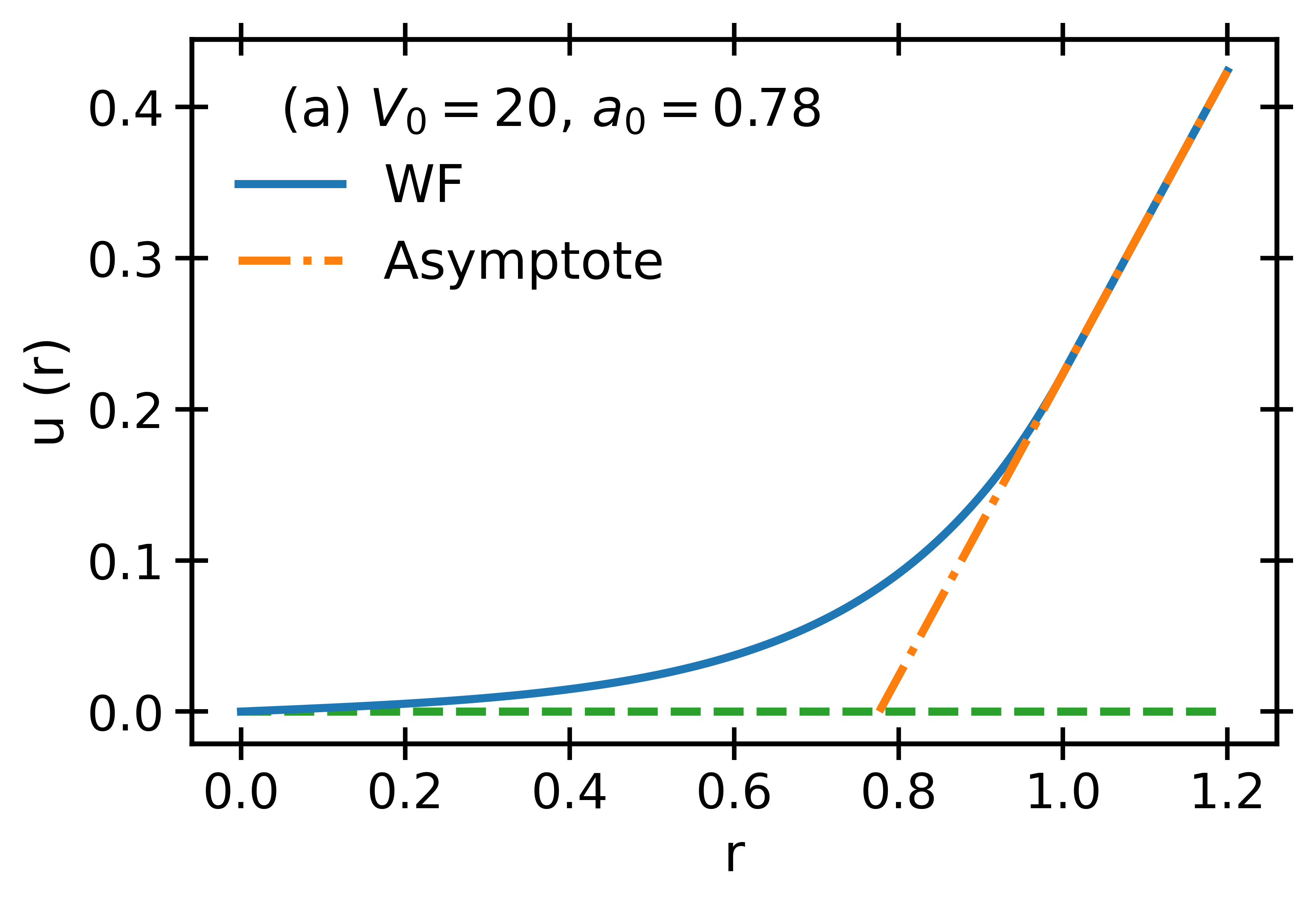
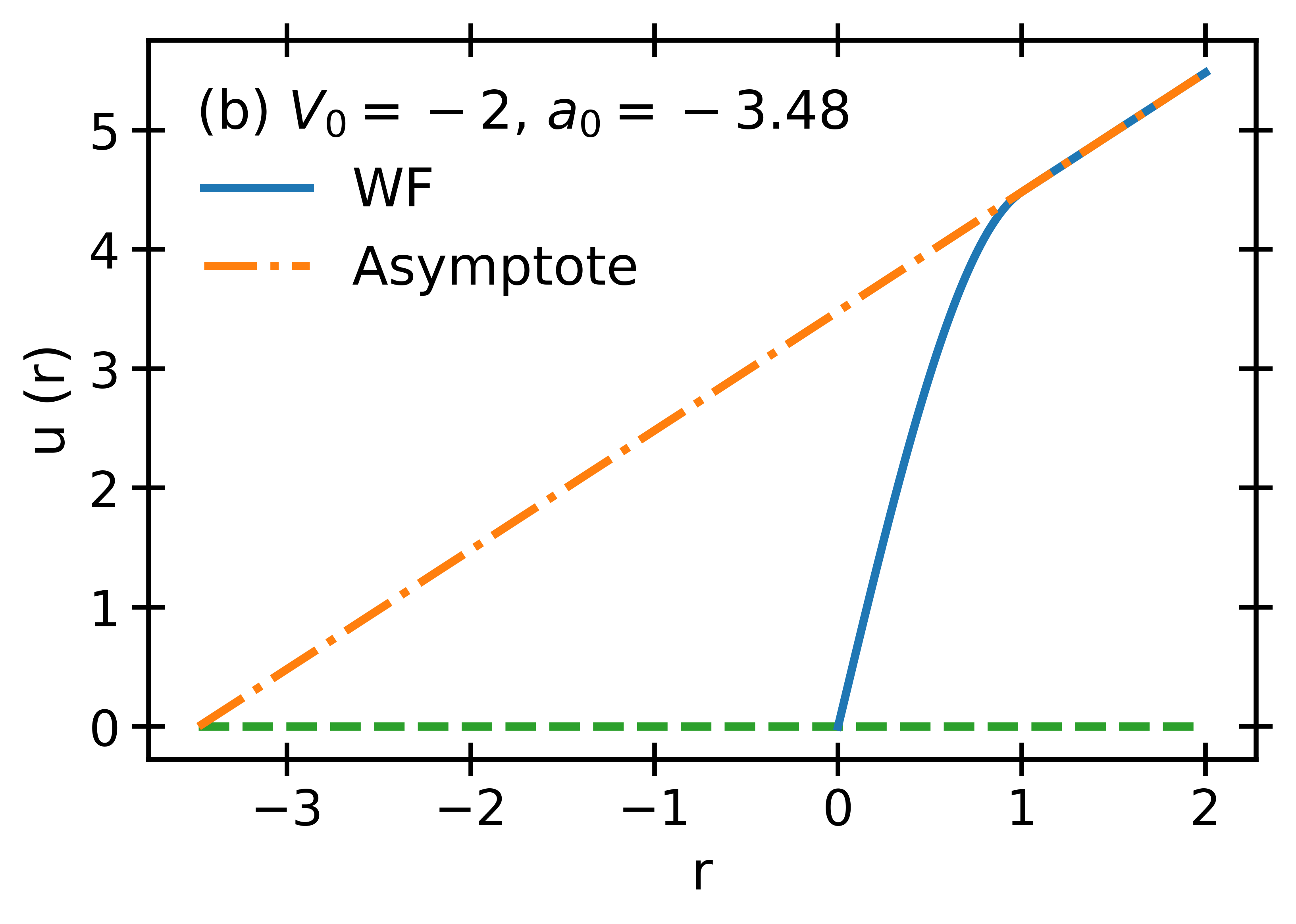
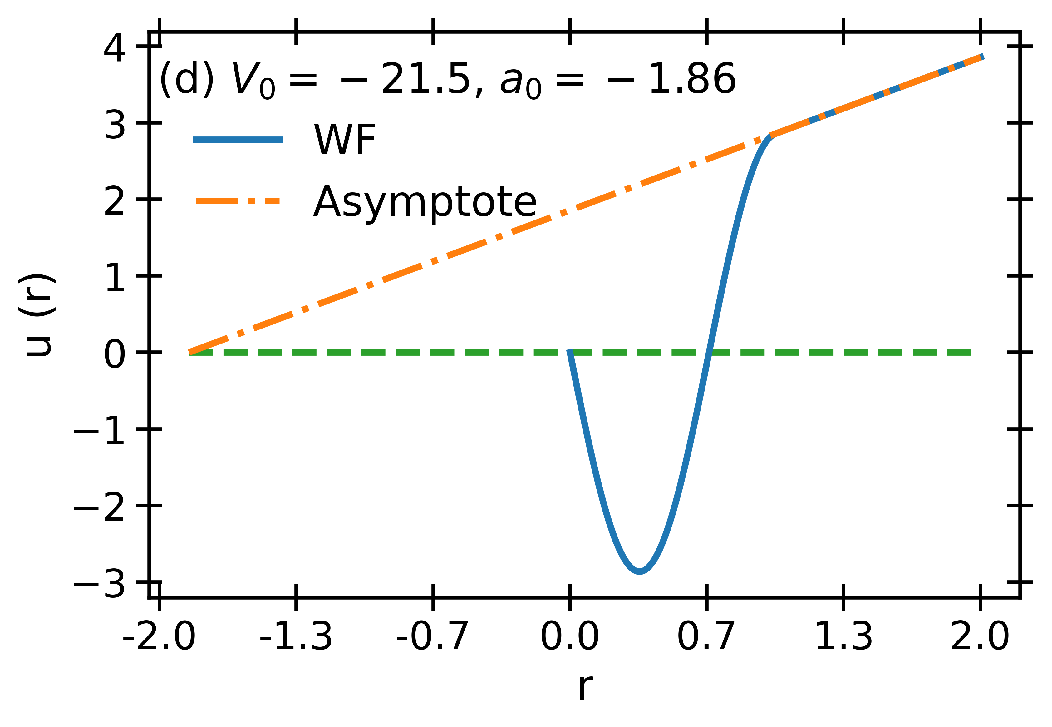
Figure 1: The wave functions (solid blue lines) are shown for four different potentials, along with linear approximations to their behavior at large $r$ (orange dotted lines). The point at which the linear approximation crosses zero yields the value of the scattering length, $a_{0}$. The potentials are all zero for $r>1$ and take the values $V_{0}$=20, -2, -5, and -21.5 for $r<1$.

We want to analyze the critical point, that is, the situation in which the scattering length diverges, going from negative to positive infinity. The Schrödinger equation always has two kind of solutions: scattering states and bound states. Scattering states can have any positive energy and at infinity behave like a non-normalizable wave. Bound states form a discrete set of solutions that have negative energy, vanish at infinity, and are normalizable. Upon increasing the strength of an attractive potential, as bound states are discrete, there will be certain values in which a scattering state with very low energy will become a bound state with negative energy close to zero. As bound states vanish at infinity, they cannot be described with the large-distance solution ($u_{l}(r)=r^{l+1}-a_{l}^{2l+1}r^{-l}$) that we have used to this point. The large-distance solution of a bound state is $Nr^{-l}$, with $N=0$ if $l=0$. In order to be able to normalize the mode, the term $a_{l}^{2l+1}r^{-l}$ should dominate $r^{l+1}$. This anomaly causes the scattering length to diverge. In fact, in this very limit (called the unitary limit) the scattering length is undefined because it can be $\pm\infty$. This process in which a scattering state transitions to a bound state as the scattering length diverges from negative to positive infinity due to an increasingly attractive potential is called a Feshbach resonance [8].

This divergent behavior around certain values of the potential can be modelled if we Taylor-expand the inverse of the scattering length around these values:

$$\frac{1}{a_{l}}(V_{0})=\frac{1}{a_{l}}\bigg{|}_{V_{c}}+\bigg{(}\frac{1}{a_{l}}\bigg{)}^{\prime}\bigg{|}_{V_{c}}(V_{0}-V_{c})+\frac{1}{2}\bigg{(}\frac{1}{a_{l}}\bigg{)}^{\prime\prime}\bigg{|}_{V_{c}}(V_{0}-V_{c})^{2}+\ldots$$ (56)

Requiring that the inverse of the scattering length at these values is zero, and ignoring orders higher than 1, we obtain:

$$a_{l}=\frac{C}{V_{0}-V_{c}}\quad\text{where}\quad C=\bigg{[}\bigg{(}\frac{1}{a_{l}}\bigg{)}^{\prime}\bigg{|}_{V_{c}}\bigg{]}^{-1}$$ (57)

Feshbach resonances appear when the energy of a scattering state matches the energy of a bound state. Although in the procedure explained above we have crossed the resonance by means of increasing the strength of the potential, we can leave the potential unchanged and make use of external sources such as magnetic fields to vary the effective interaction and cross the resonance either-way. Magnetically tunable Feshbach resonances are very important in ultracold quantum gases. Their use provides means of varying the scattering length almost at will. [14] For instance, one can go from a Fermi gas with pairing (BCS) with $a<0$ to a Bose-Einstein condensate (BEC) with $a>0$ by crossing a Feshbach resonance. [15]

As we have found a compact formula for the effective range, it is interesting to explore the behavior of the effective range whenever $a_{l}$ is zero or $\pm\infty$. The case $a_{l}=0$ is only interesting from a mathematical point of view. Physically, it is not relevant because what matters is the product of $r_{l}^{\text{eff}}$ times $a_{l}^{2l+2}$. This product is the constant $c_{2}$ introduced in Sec. II, which is one of the coefficients of the expansion of the tangent of the phase shift. On the other hand, the case $a_{l}=\pm\infty$ is physically important, since this corresponds to the behavior around the Feshbach resonance. To this end, we write a compact expression of $r_{l}^{\text{eff}}$:

$$r_{l}^{\text{eff}}=\frac{2}{(2l+1)a_{l}^{2l+2}}\int_{0}^{\infty}\Big{[}r^{2l+2}-2a_{l}^{2l+1}r+a_{l}^{4l+2}r^{-2l}\delta_{l,0}-{u_{l}^{(0)}}^{2}(r)\Big{]}dr\ .$$ (58)

First, we analyze its behavior when $a_{l}\to 0$. By looking at the dominant terms in this limit, one gets:

$$r_{l}^{\text{eff}}\rightarrow\frac{2}{(2l+1)a_{l}^{2l+2}}\int_{0}^{\infty}\Big{[}r^{2l+2}-{u_{l}^{(0)}}^{2}(r)\Big{]}dr\rightarrow\pm\infty\ .$$ (59)

The integral in Eq. (59) is always finite unless $a_{l}$ diverges. For the case where $a_{l}$ does not diverge, the effective range can only diverge if the fraction preceding the integral diverges, which would necessarily be due to $a_{l}^{2l+2}$. However, since the product of $a_{l}^{2l+2}$ and $r_{l}^{\text{eff}}$ is finite,

$$r_{l}^{\text{eff}}a_{l}^{2l+2}\rightarrow\frac{2}{(2l+1)}\int_{0}^{\infty}\Big{[}r^{2l+2}-{u_{l}^{(0)}}^{2}(r)\Big{]}dr\ ,$$ (60)

this limit (Eq. (59)) is not physically relevant. We recall that the product $r_{l}^{\text{eff}}a_{l}^{2l+2}$ is what appears in the expansion of the tangent of delta, see Eqs. (28) and (30).

When considering the case in which $a_{l}\to\pm\infty$, it is useful to split the wave function into two terms (the derivation of which is found in Sec. IV of the Supplementary material I [13]):

$$u_{l}^{(0)}(r)=\frac{lu_{l}^{(0)}(r)+r{u^{\prime}}_{l}^{(0)}(r)}{1+2l}-\frac{r{u^{\prime}}_{l}^{(0)}(r)-(l+1)u_{l}^{(0)}(r)}{1+2l}\ .$$ (61)

The first term goes to positive infinity as $r^{l+1}$ while the second term goes to positive infinity as $a_{l}^{2l+1}r^{-l}$. We recall that at infinity $u_{l}^{(0)}(r)$ is $r^{l+1}-a_{l}^{2l+1}r^{-l}$. As long as $a_{l}$ is non-zero, we can redefine the two parts as two functions:

$$\frac{lu_{l}^{(0)}(r)+r{u^{\prime}}_{l}^{(0)}(r)}{1+2l}\equiv f_{l}(r)\quad;\quad\frac{r{u^{\prime}}_{l}^{(0)}(r)-(l+1)u_{l}^{(0)}(r)}{1+2l}\equiv a_{l}^{2l+1}h_{l}(r)\ .$$ (62)

Both $f_{l}(r)$ and $h_{l}(r)$ at $r=0$ are zero. And at $r\to\infty$, they are $r^{l+1}$ and $r^{-l}$ respectively. The differential equations that $f_{l}(r)$ and $h_{l}(r)$ satisfy can be found in Sec. IV of the Supplementary material I [13]. With this, the wave function can be rewritten as $u_{l}^{(0)}(r)=f_{l}(r)-a_{l}^{2l+1}h_{l}(r)$. If we apply this transformation to the effective range, we obtain:

$$r_{l}^{\text{eff}}=\frac{2}{(2l+1)a_{l}^{2l+2}}\bigg{\{}\int_{0}^{\infty}\Big{[}r^{2l+2}-f_{l}^{2}(r)\Big{]}dr-2a_{l}^{2l+1}\int_{0}^{\infty}\Big{[}r-f_{l}(r)h_{l}(r)\Big{]}+a_{l}^{4l+2}\int_{0}^{\infty}\Big{[}r^{-2l}\delta_{l,0}-h_{l}^{2}(r)\Big{]}dr\bigg{\}}\ .$$ (63)

The above integrals are finite. This can be seen by noting that $f_{l}^{2}(0)$, $f_{l}(0)h_{l}(0)$, and $h_{l}^{2}(0)$ are zero, and that $\lim_{r\rightarrow\infty}\Big{[}r^{2l+2}-f_{l}^{2}(r)\Big{]}=0$, $\lim_{r\rightarrow\infty}\Big{[}r-f_{l}(r)h_{l}(r)\Big{]}=0$, and $\lim_{r\rightarrow\infty}\Big{[}r^{-2l}\delta_{l,0}-h_{l}^{2}(r)\Big{]}=0$.

We distinguish two cases, $l=0$ and $l>0$. In the first case, when $a_{0}\to\pm\infty$:

$$r_{0}^{\text{eff}}\rightarrow 2\int_{0}^{\infty}\Big{[}1-h_{l}^{2}(r)\Big{]}dr\rightarrow\text{finite value}\ .$$ (64)

Instead, for $l>0$ and $a_{l}\to\pm\infty$:

$$r_{l}^{\text{eff}}\rightarrow-\frac{2}{(2l+1)}a_{l}^{2l}\int_{0}^{\infty}h_{l}^{2}(r)dr\rightarrow-\infty\ .$$ (65)

As a summary, whenever $a_{l}$ is zero, $r_{l}^{\text{eff}}$ diverges. For a diverging scattering length, we have two situations: for $l=0$, the effective range is finite, while for $l>0$, it diverges to $-\infty$.

V Examples

In this section, we apply the scattering formalism to obtain the scattering length and effective ranges of model potentials that can be analytically integrated. We just present the final formulas, the development can be found in the Supplementary material II. [12] Moreover, in Sup. Mat. II [12], we have computed the parameters for the Pöschl-Teller potential. However, this case has been done numerically, not analytically, and this is why it is not presented here.

V.1 Hard-sphere potential

The hard-sphere potential is one of the simplest potential models. It only has one parameter, which is the size of the repulsive core. We point out that the formulas derived in Sec. III do not work for this particular potential due to its divergent behavior at the core. The well-known hard-sphere potential is given by

$$V(r)=\begin{cases}\infty&\mbox{if}\quad r\leq R\\ 0&\mbox{if}\quad r>R\ .\end{cases}$$ (66)

The wave function is zero for $r\leq R$ and

$$u_{l}(r>R)=\frac{Nk^{-l}}{A_{l}}r\bigg{[}j_{l}(kr)-n_{l}(kr)\tan{\delta}\bigg{]}$$ (67)

for $r>R$. We recall that $k=\sqrt{2\mu E/\hbar^{2}}$. The scattering length and effective range for any angular momentum $l$ are:

$$a_{l} = R$$ (68)

$$r_{l} = -\bigg{(}\frac{1}{(2l+3)}+\frac{1}{(2l-1)}\bigg{)}R\ ,$$ (69)

with $a_{l}$ being the scattering length and $r_{l}$ the effective range (hereafter, we have eliminated the superscript “eff” in the effective range to simplify the notation). As we can see, for hard spheres the scattering length is $R$ at any $l$, whereas the effective range is also proportional to $R$ with a value that is positive only for $l=0$, $r_{0}=2/3R$.

V.2 Soft-sphere potential

In contrast to the hard-sphere interaction, the soft-sphere potential takes into account that the core, although being repulsive, may be penetrated. This correction results in the model potential having two parameters: the strength of the potential and the core size. The soft-sphere potential is given by

$$V(r)=\begin{cases}V_{0}&\mbox{if}\quad r\leq R\\ 0&\mbox{if}\quad r>R\ .\end{cases}$$ (70)

For $r\leq R$ , the Schrödinger equation is:

$$u_{l}^{\prime\prime}(r)+\bigg{(}\overline{k}^{2}-\frac{l(l+1)}{r^{2}}\bigg{)}u_{l}(r)=0\quad\text{where}\quad\overline{k}^{2}=\frac{2\mu}{\hbar^{2}}(E-V_{0})\ ,$$ (71)

with $\overline{k}=\sqrt{k^{2}-k_{0}^{2}}$, a complex number for energies $E<V_{0}$. We have defined $k_{0}$ as $\sqrt{2\mu V_{0}/\hbar^{2}}$. In order to have a real function, we need to multiply the Bessel function with an imaginary argument by $i^{-l}$:

$$u_{l}(r)=Nrj_{l}(\overline{k}r)i^{-l}\ .$$ (72)

For $r>R$ and $k\to 0$, we know the asymptotic solution (see Sec II) is:

$$u_{l}(r,k=0)=r^{l+1}-a_{l}^{2l+1}r^{-l}\ .$$ (73)

By imposing that the wave function is continuous at $r=R$, we can find the normalization constant $N$:

$$N=\frac{R^{l+1}-a_{l}^{2l+1}R^{-l}}{Ri^{-l}j_{l}(ik_{0}R)}\ .$$ (74)

After applying the formulas we have derived in Sec. III, we can obtain the scattering length $a_{l}$:

$$a_{l}^{2l+1}=R^{2l+1}\frac{k_{0}Ri^{-l-1}j_{l+1}(ik_{0}R)}{(2l+1)i^{-l}j_{l}(ik_{0}R)+k_{0}Ri^{-l-1}j_{l+1}(ik_{0}R)}\ .$$ (75)

The effective range for any $l$ is:

$$r_{l}=\frac{2}{(2l+1)a_{l}^{2l+2}}\bigg{\{}\frac{R^{2l+3}}{2l+3}-a_{l}^{2l+1}R^{2}+\frac{a_{l}^{4l+2}R^{1-2l}}{1-2l}-N^{2}(i^{-l})^{2}\frac{1}{2}R^{3}\Big{(}j_{l}^{2}(ik_{0}R)-j_{l-1}(ik_{0}R)j_{l+1}(ik_{0}R))\Big{)}\bigg{\}}\ .$$ (76)

From the general results (75) and (76), we can find the expressions for $l=0$ and $l=1$ by introducing the Bessel functions explicitly. The scattering lengths are:

$$a_{0} = R\bigg{[}1-\frac{\tanh{(k_{0}R)}}{k_{0}R}\bigg{]}\ ,$$ (77)

$$a_{1}^{3} = R^{3}\bigg{[}\frac{3+(k_{0}R)^{2}-3k_{0}R\coth{(k_{0}R)}}{(k_{0}R)^{2}}\bigg{]}\ ,$$ (78)

and the effective ranges are:

$$r_{0} = R-R\frac{(k_{0}R)^{2}}{3(k_{0}R)^{2}\bigg{(}1-\cfrac{\tanh{(k_{0}R)}}{k_{0}R}\bigg{)}^{2}}+R\frac{1}{(k_{0}R)^{2}\bigg{(}1-\cfrac{\tanh{(k_{0}R)}}{k_{0}R}\bigg{)}}\ ,$$ (79)

$$r_{1} = -3k_{0}a_{1}^{2}\frac{-2k_{0}R(-5+(k_{0}R)^{2})+2k_{0}R(10+(k_{0}R)^{2})\cosh{(2k_{0}R)}-5(3+2(k_{0}R)^{2})\sinh{(2k_{0}R)}}{10\bigg{(}-3k_{0}R\cosh{(k_{0}R)+(3+(k_{0}R)^{2})\sinh{(k_{0}R)}}\bigg{)}^{2}}\ .$$ (80)

In Fig. 2, we plot the functions (77,78,79,80). The scattering lengths $a_{0}$ and $a_{1}$ are zero when $k_{0}R$ is zero, and are equal to $R$ (hard-spheres solution) when $k_{0}R$ becomes large. In contrast, $r_{0}$ and $r_{1}$ diverge for $k_{0}R$ equal to zero, and when $k_{0}R$ increases we recover the value of hard-spheres, which is $2R/3$ and $-6R/5$, respectively.

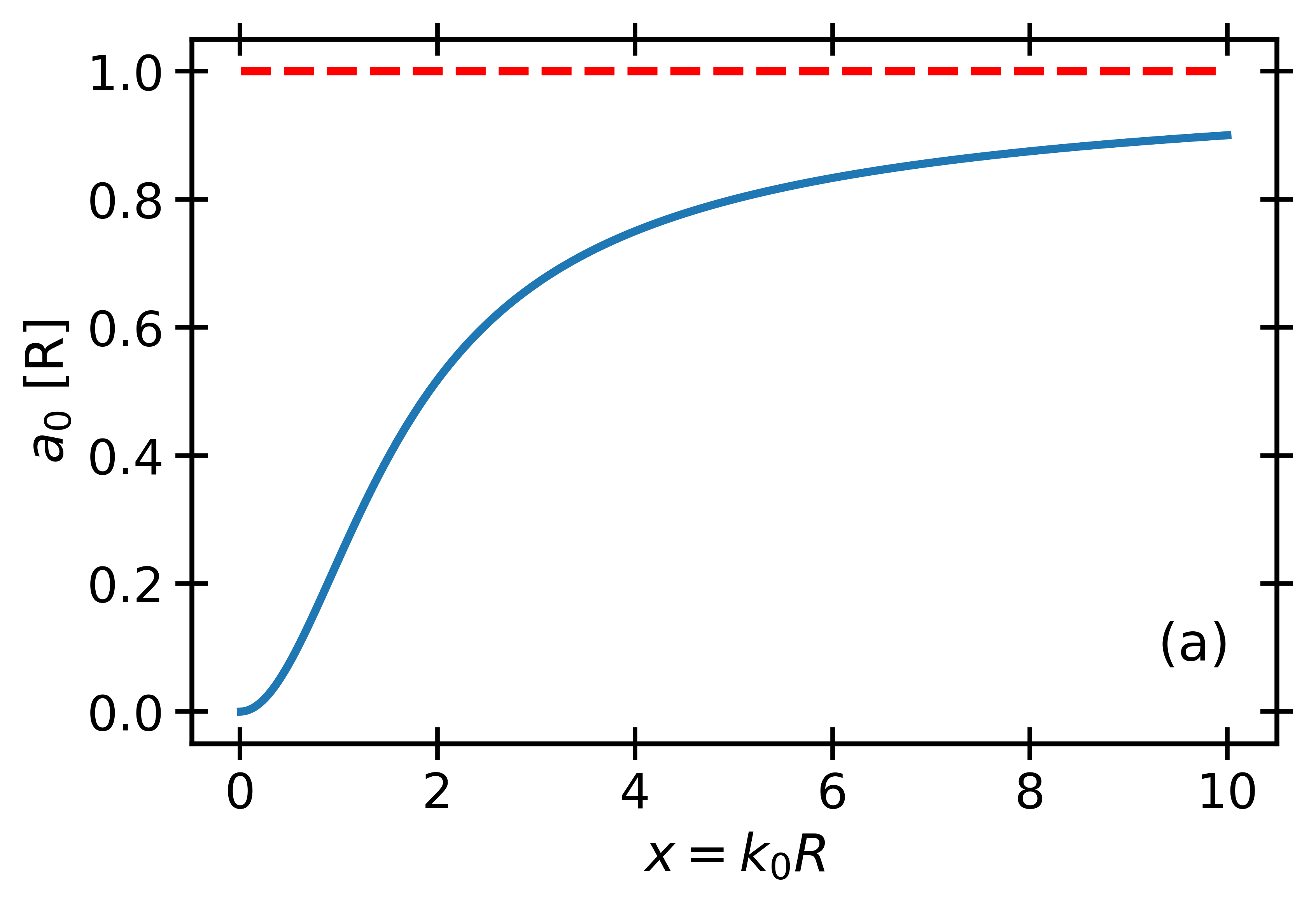
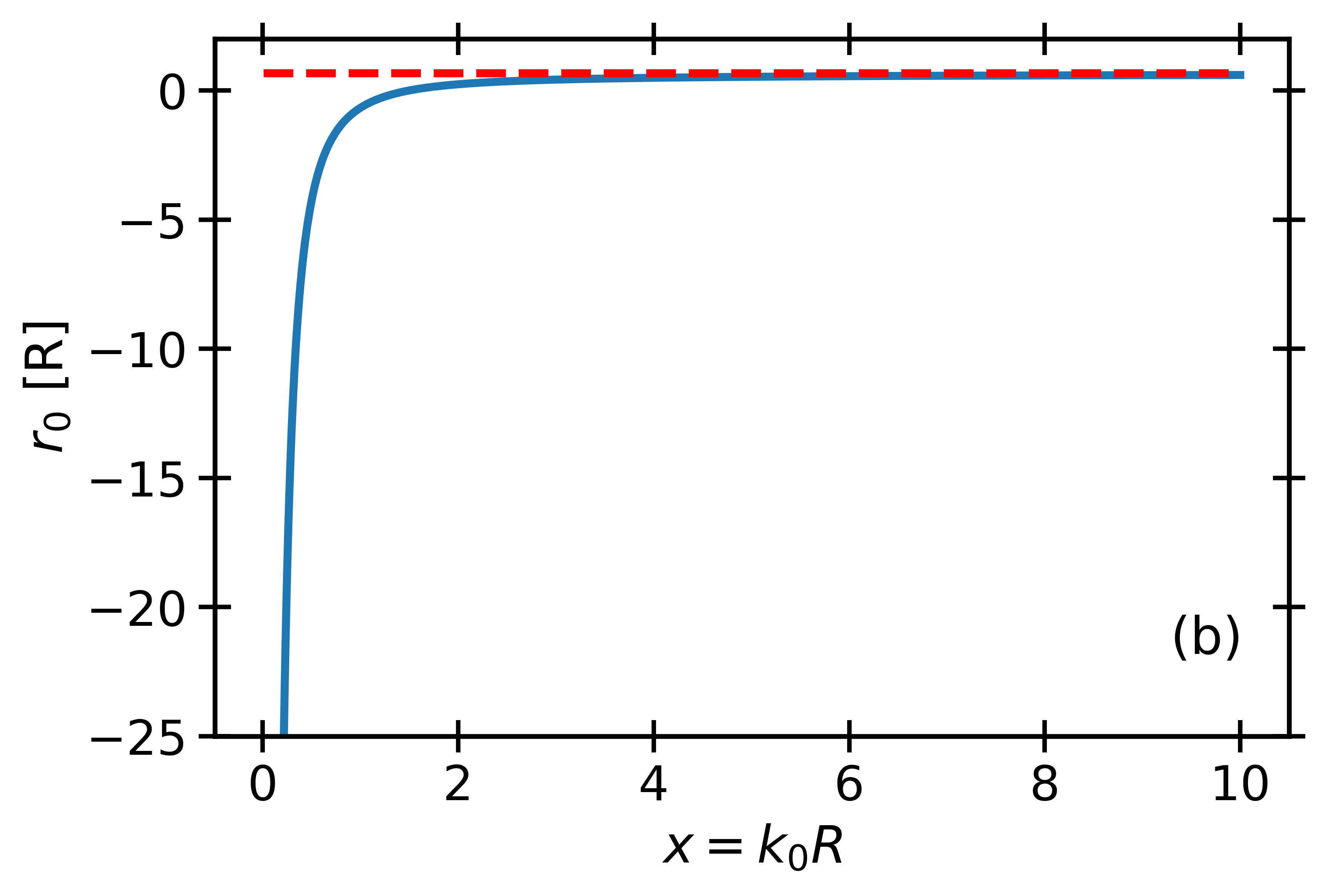
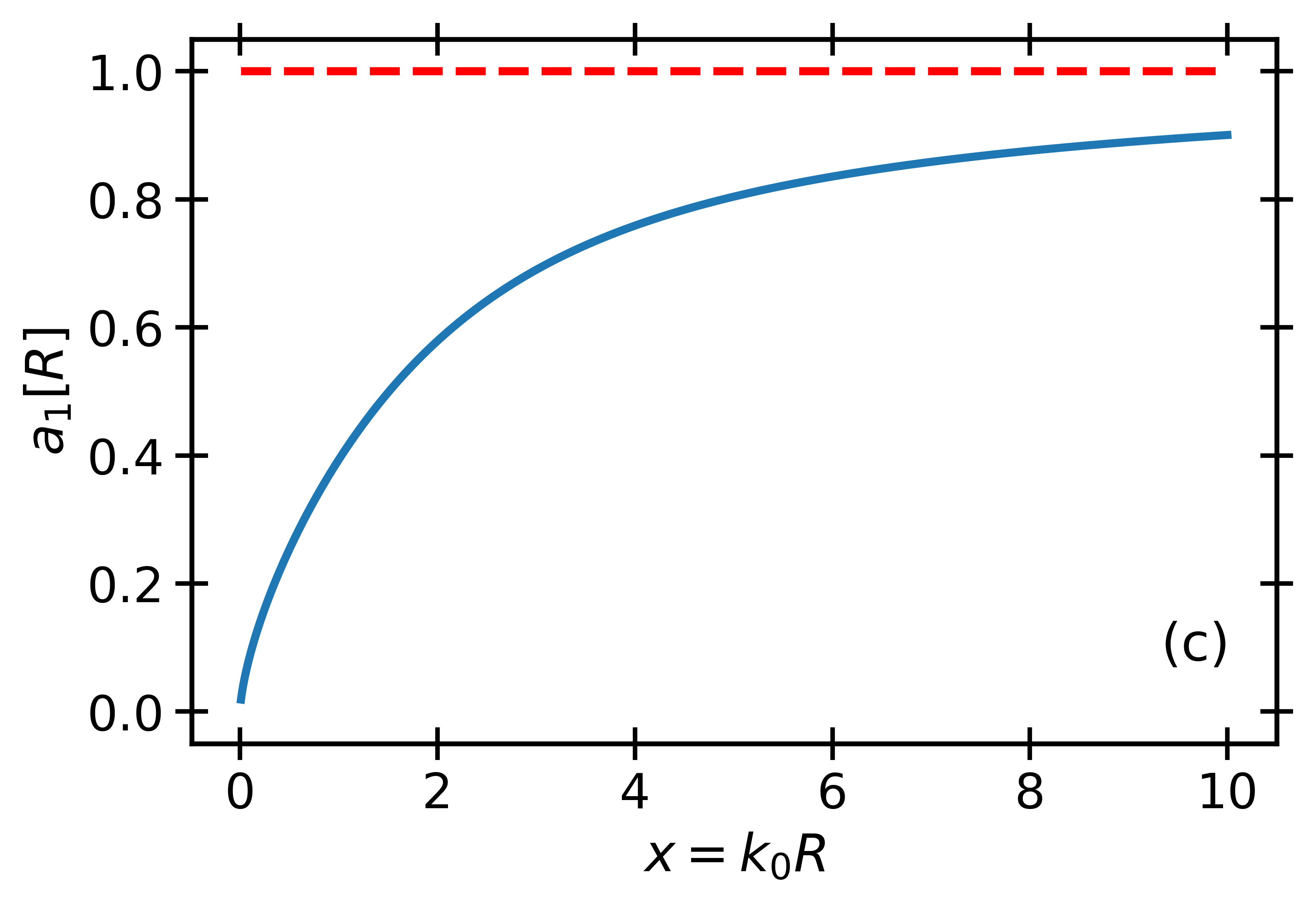
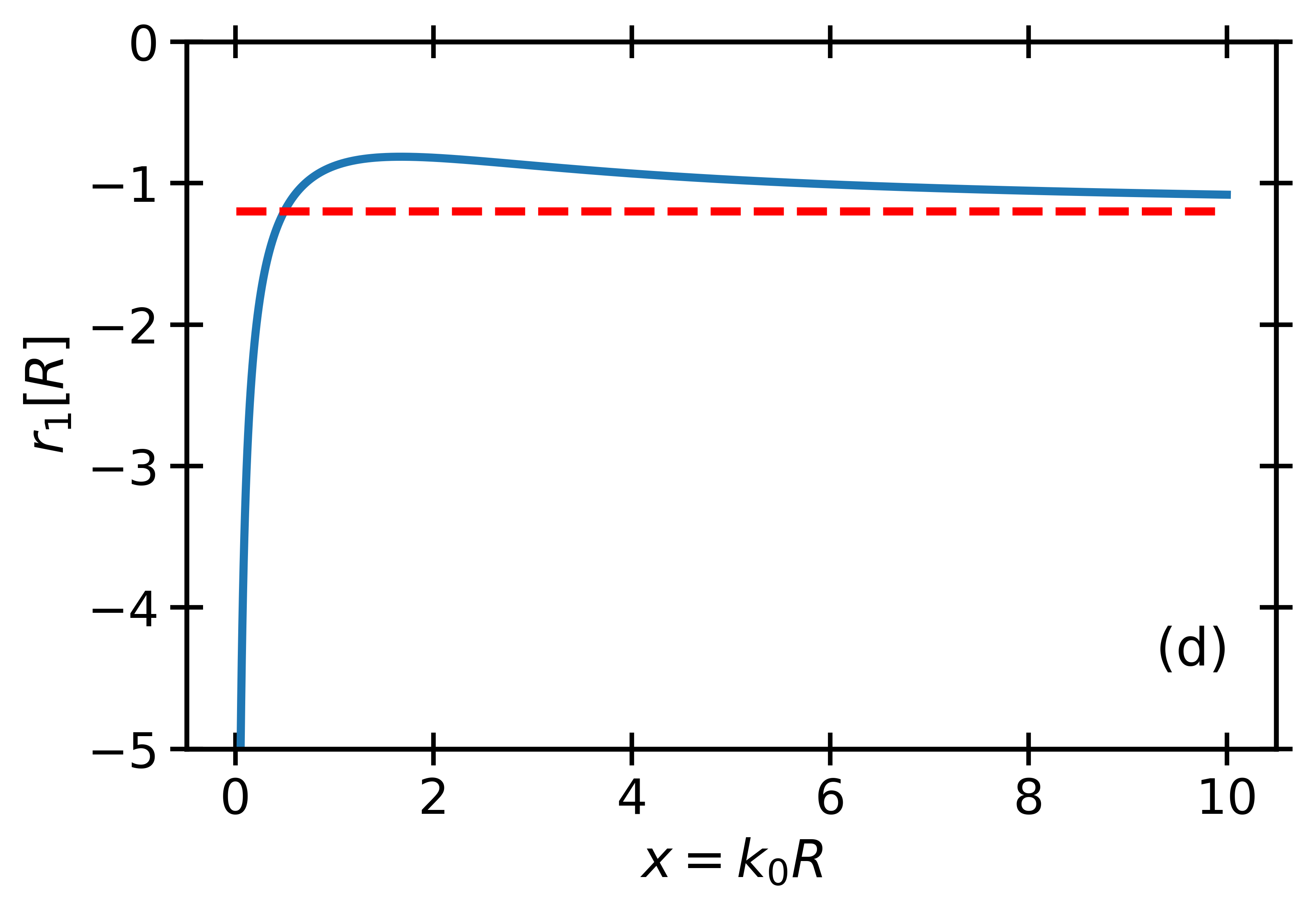
Figure 2: $a_{0}$, $r_{0}$, $a_{1}$ and $r_{1}$ for a soft-sphere potential as a function of $k_{0}R$. The red dashed lines correspond to the hard-sphere limit.

An alternate way of finding the scattering parameters of the soft-sphere potential is shown in the Appendix of the Supplemental Material II [12].

V.3 Spherical well potential

In the previous Section, we solved the soft-sphere model potential, where we have a potential barrier. The spherical well potential is the same idea of the soft-sphere potential but taking it as an attractive potential,

$$V(r)=\begin{cases}-V_{0}&\mbox{if}\quad r\leq R\\ 0&\mbox{if}\quad r>R\ .\end{cases}$$ (81)

For the spherical well, where the potential is negative, we can use the expressions that we have obtained for soft-spheres by simply changing $k_{0}$ to $-ik_{0}$. Note that since $k_{0}$ depends on the square root of $V_{0}$, a sign change in $V_{0}$ results in $k_{0}$ becoming imaginary. If we apply this change in sign to $V_{0}$, then we arrive easily to the general formulas for any $l$. For the lowest partial waves $l=0$ and $l=1$, the scattering lengths are:

$$a_{0} = R\bigg{[}1-\frac{\tan{(k_{0}R)}}{k_{0}R}\bigg{]}\ ,$$ (82)

$$a_{1}^{3} = R^{3}\bigg{[}\frac{(k_{0}R)^{2}-3+3k_{0}R\cot{(k_{0}R)}}{(k_{0}R)^{2}}\bigg{]}\ ,$$ (83)

and the effective ranges are:

$$r_{0} = R-R\frac{(k_{0}R)^{2}}{3(k_{0}R)^{2}\bigg{(}1-\cfrac{\tan{(k_{0}R)}}{k_{0}R}\bigg{)}^{2}}-R\frac{1}{(k_{0}R)^{2}\bigg{(}1-\cfrac{\tan{(k_{0}R)}}{k_{0}R}\bigg{)}}\ ,$$ (84)

$$r_{1} = -3k_{0}a_{1}^{2}\frac{2k_{0}R(5+(k_{0}R)^{2})+2k_{0}R(10-(k_{0}R)^{2})\cos{(2k_{0}R)}-5(3-2(k_{0}R)^{2})\sin{(2k_{0}R)}}{10\bigg{(}3k_{0}R\cos{(k_{0}R)-(3-(k_{0}R)^{2})\sin{(k_{0}R)}}\bigg{)}^{2}}\ .$$ (85)

As we discussed in Sec. IV, in an attractive potential and at certain values of the potential strength, the scattering length diverges (Feshbach resonance). That means that a bound state appears. For the spherical well potential, the resonance for $l=0$ occurs at $k_{0}R=(2n-1)\pi/2$ and for l=1 at $k_{0}R=n\pi$, with $n\geq 1$. In Fig. 3, we plot the scattering lengths and effective ranges for $l=0$ and $l=1$. We observe the predicted divergences: $a_{0}$ diverges at $k_{0}R=$ $\pi$/2, 3$\pi$/2 and 5$\pi$/2. $a_{1}$ diverges at $k_{0}R=$ $\pi$, 2$\pi$ and 3$\pi$.

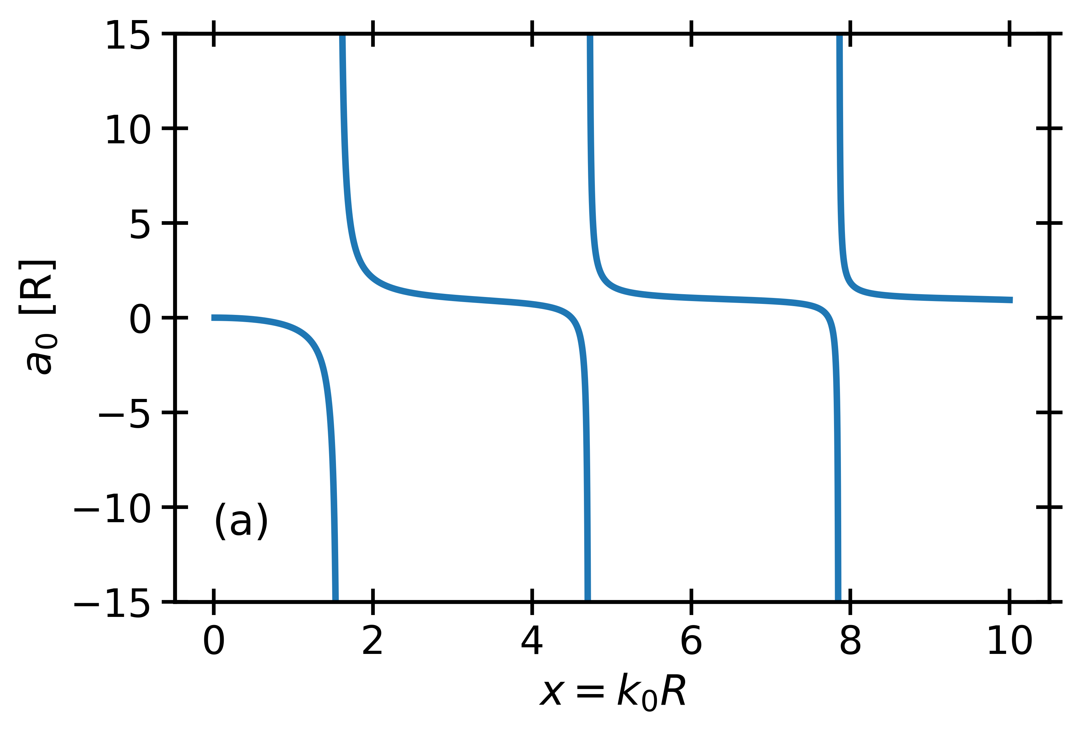
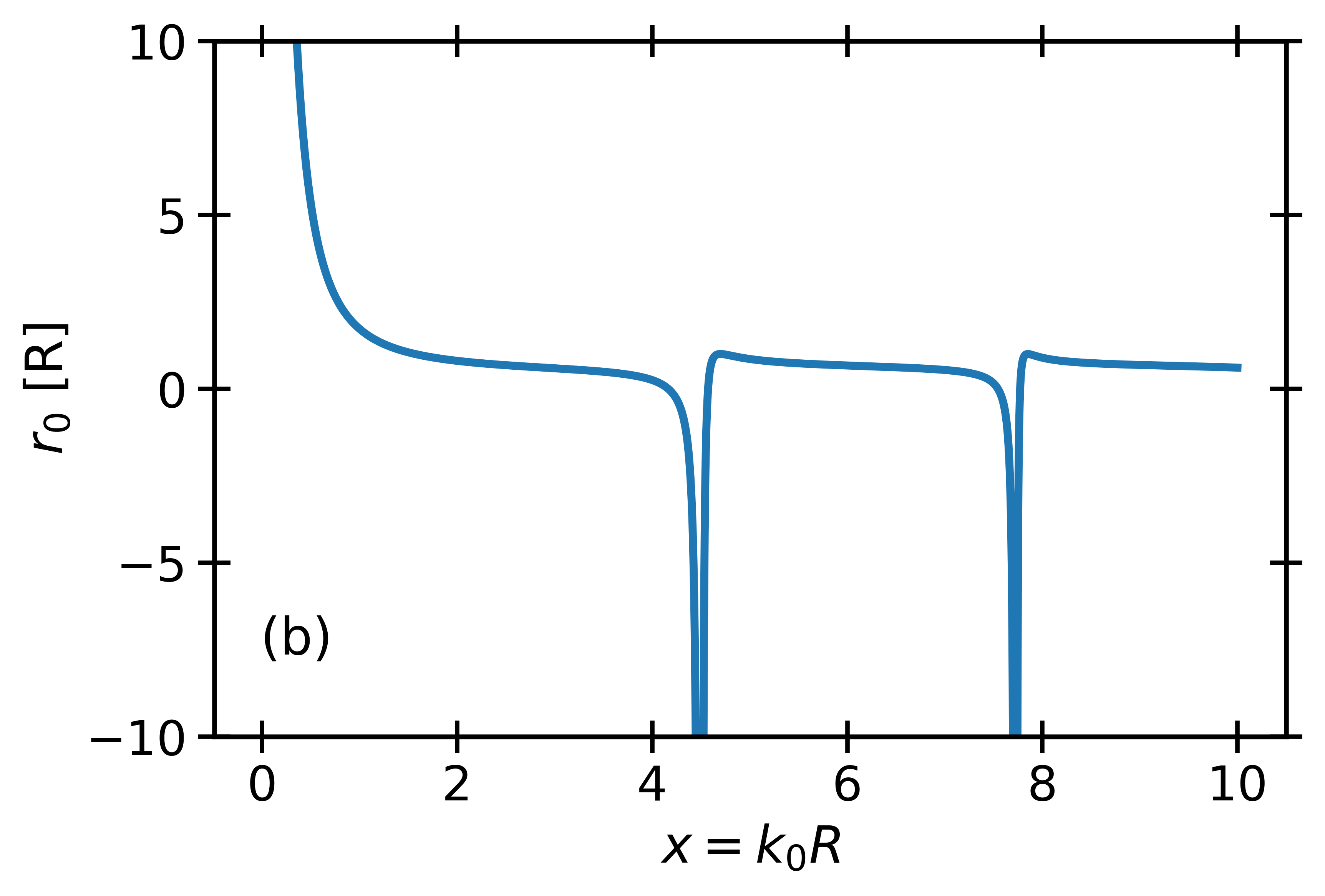
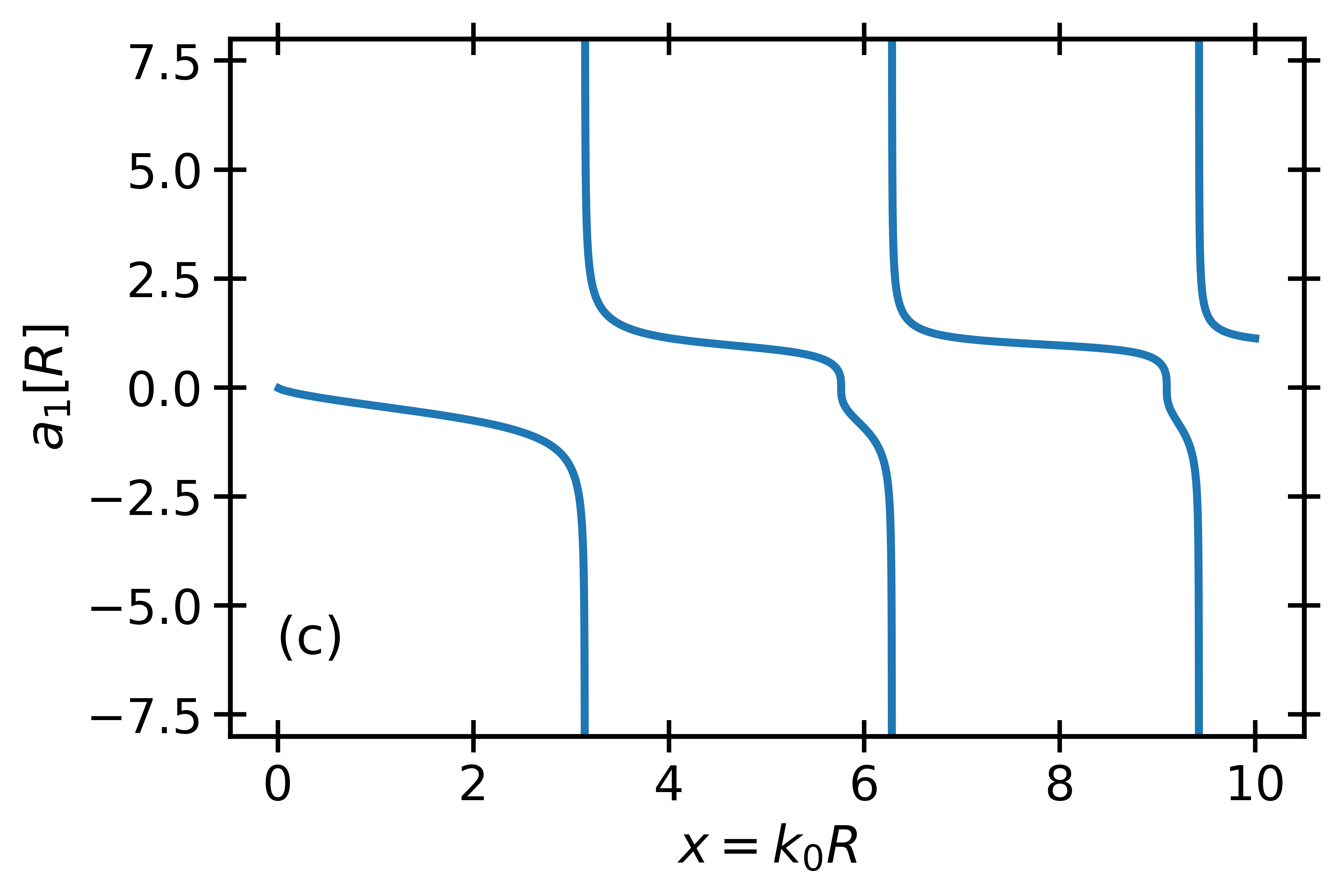
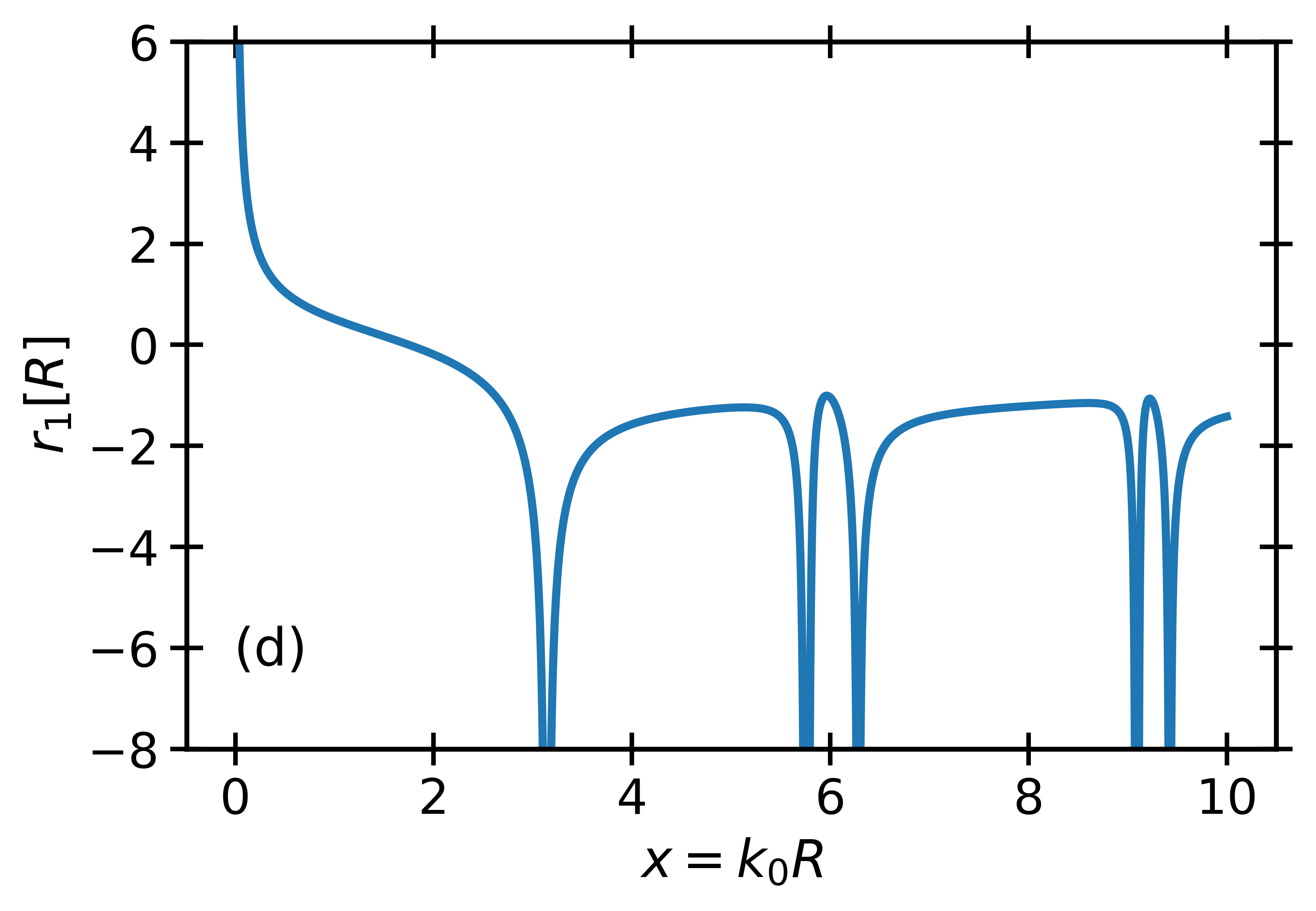
Figure 3: Representation of $a_{0}$, $r_{0}$, $a_{1}$ and $r_{1}$ for a spherical well.

If one looks to the shape of the effective ranges, one can see some divergences appearing. As we proved in the end of Sec. IV, the divergences of the effective ranges are related to the divergences of the scattering length and to its zero value. In particular, for $r_{0}$ the divergences occur when $a_{0}=0$, while for $r_{1}$, we see divergences coming from both limits, that is when $a_{1}=0$ and $a_{1}=\pm\infty$. From that, we can also understand why we were not seeing a divergence in the effective range, $r_{0}$, near the region of the first divergence of the scattering length. This is because, before the first divergence of $a_{0}$, $a_{0}$ is already negative and we do not see a change in the sign (hence, passing through zero) until we go to the second divergence of $a_{0}$.

V.4 Well-barrier potential

This model potential is more involved than the previous ones. It is a combination of a spherical-well potential and a soft-sphere (barrier) potential. Due to this combination, with this model potential we have four parameters at our disposal: the strengths and the sizes of the spherical-well and the barrier. This model potential is very well suited when working with perturbative expansions of many-body systems that contain the three most important scattering parameters ($a_{0}$, $a_{1}$ and $r_{0}$) as it more easily fits them than in the previous model potentials. It is given by

$$V(r)=\begin{cases}-V_{1}&\mbox{if}\quad r\leq R_{1}\\ V_{2}&\mbox{if}\quad R_{1}<r\leq R_{2}\\ 0&\mbox{if}\quad r>R_{2}\ .\end{cases}$$ (86)

In the internal region we have a well potential, in which the wave function will be the regular Bessel function with a real argument:

$$u_{l}^{(0)}(r)=N_{1}rj_{l}(k_{1}r)\quad\text{if}\quad r\leq R_{1},\quad\text{where}\quad k_{1}=\sqrt{2\mu V_{1}/\hbar^{2}}\ .$$ (87)

In the second region, the solution is a combination of Bessel functions with imaginary arguments, just like in the barrier potential:

$$u_{l}^{(0)}(r)=N_{2}r\Big{[}j_{l}(ik_{2}r)+M_{2}n_{l}(ik_{2}r)\Big{]}\quad\text{if}\quad R_{1}<r\leq R_{2},\quad\text{where}\quad k_{2}=\sqrt{2\mu V_{2}/\hbar^{2}}\ .$$ (88)

And finally, beyond $R_{2}$, we have the long-distance solution:

$$u_{l}^{(0)}(r)=r^{l+1}-a_{l}^{2l+1}r^{-l}\quad\text{if}\quad r>R_{2}\ .$$ (89)

We need the constants of integration:

$$N_{1}=N_{2}\frac{j_{l}(ik_{2}R_{1})+M_{2}n_{l}(ik_{2}R_{1})}{j_{l}(k_{1}R_{1})}\quad;\quad N_{2}=\frac{R_{2}^{l+1}-a_{l}^{2l+1}{R_{2}}^{-l}}{R_{2}\big{[}j_{l}(ik_{2}R_{2})+M_{2}n_{l}(ik_{2}R_{2})\big{]}}$$ (90)

$$\text{and}\quad M_{2}=-\frac{ik_{2}R_{1}j_{l}(k_{1}R_{1})j_{l+1}(ik_{2}R_{1})-k_{1}R_{1}j_{l}(ik_{2}R_{1})j_{l+1}(k_{1}R_{1})}{ik_{2}R_{1}j_{l}(k_{1}R_{1})n_{l+1}(ik_{2}R_{1})-k_{1}R_{1}n_{l}(ik_{2}R_{1})j_{l+1}(k_{1}R_{1})}\ .$$ (91)

The $l$-wave scattering length is:

$$a_{l}^{2l+1}=\frac{R_{2}^{2l+1}\displaystyle\int_{0}^{R_{2}}U(r)r^{l+1}u_{l}^{(0)}(r)dr}{(2l+1)R_{2}^{l}u_{l}^{(0)}(R_{2})+\displaystyle\int_{0}^{R_{2}}U(r)r^{l+1}u_{l}^{(0)}(r)dr}\ ,$$ (92)

where $u_{l}^{(0)}(R_{2})$ is $N_{2}R_{2}\Big{[}j_{l}(ik_{2}R_{2})+M_{2}n_{l}(ik_{2}R_{2})\Big{]}$ and the integrals are:

$$\int_{0}^{R_{2}}U(r)r^{l+1}u_{l}^{(0)}(r)dr=-N_{1}k_{1}R_{1}^{l+2}j_{l+1}(k_{1}r)-iN_{2}k_{2}\bigg{[}r^{l+2}j_{l+1}(ik_{2}r)+M_{2}(-1)^{l}r^{l+2}j_{-l-2}(ik_{2}r)\bigg{]}_{R_{1}}^{R_{2}}\ .$$ (93)

Finally, the effective range can be written as

$$r_{l}=\frac{2}{(2l+1)a_{l}^{2l+2}}\bigg{\{}\frac{R_{2}^{2l+3}}{2l+3}-a_{l}^{2l+1}R_{2}^{2}+\frac{a_{l}^{4l+2}R_{2}^{1-2l}}{1-2l}-N_{1}^{2}I_{jj}(k_{1}R_{1})-N_{2}^{2}\bigg{[}I_{jj}(ik_{2}r)+M_{2}^{2}I_{nn}(ik_{2}r)+2M_{2}I_{jn}(ik_{2}r)\bigg{]}_{R_{1}}^{R_{2}}\bigg{\}}\ .$$ (94)

The functions $I_{jj}(kr)$, $I_{nn}(kr)$ and $I_{jn}(kr)$ in Eq. (94) are:

$$I_{jj}(kr)=\int r^{2}j_{l}^{2}(kr)dr=\frac{r^{3}}{2}\big{(}j_{l}^{2}(kr)-j_{l-1}(kr)j_{l+1}(kr)\big{)}\ ,$$ (95)

$$I_{nn}(kr)=\int r^{2}n_{l}^{2}(kr)dr=\frac{r^{3}}{2}\big{(}n_{l}^{2}(kr)-n_{l-1}(kr)n_{l+1}(kr)\big{)}\ ,$$ (96)

$$I_{jn}(kr)=\int r^{2}j_{l}(kr)n_{l}(kr)dr=\frac{(-1)^{l}r^{3}}{2}j_{-l}(kr)j_{l-1}(kr)-\frac{(-1)^{l}r^{3}}{2}j_{-l-1}(kr)j_{l}(kr)$$ (97)

$$-\frac{(1+2l)(-1)^{l}r^{2}}{4k}j_{-l}(kr)j_{l}(kr)+\frac{(1+2l)(-1)^{l}r^{2}}{4k}j_{-l-1}(kr)j_{l-1}(kr)\ .$$

The scattering length for $l=0$ is:

$$a_{0}=\frac{\cosh{(k_{2}R_{12})}[-k_{1}k_{2}R_{2}\cos{(k_{1}R_{1})+k_{2}\sin{(k_{1}R_{1})}}]+\sinh{(k_{2}R_{12})}[k_{2}^{2}R_{2}\sin{(k_{1}R_{1})}-k_{1}\cos{(k_{1}R_{1})}]}{-k_{1}k_{2}\cos{(k_{1}R_{1})}\cosh{(k_{2}R_{12})}+k_{2}^{2}\sin{(k_{1}R_{1})}\sinh{(k_{2}R_{12})}}\ ,$$ (98)

with $R_{12}=R_{1}-R_{2}$. For $a_{1}$ and $r_{0}$, the expressions are complicated but still manageable, and hence, we can split them into parts. For $a_{1}$ we get:

$$a_{1}^{3}=\frac{p_{1}+p_{2}}{d_{1}}\ ,$$ (99)

with

$$p_{1} = \cosh{(k_{2}R_{12})}\{3k_{1}k_{2}^{3}R_{1}R_{2}^{2}\cos{(k_{1}R_{1})+k_{2}R_{2}[-3k_{2}^{2}R_{2}+k_{1}^{2}(3R_{1}-3R_{2}+k_{2}^{2}R_{1}R_{2}^{2})]\sin{(k_{1}R_{1})}}\}\ ,\hskip 52.63777pt$$ (100)

$$p_{2} = \sinh{(k_{2}R_{12})}\{k_{1}k_{2}^{2}R_{1}R_{2}[3+k_{2}^{2}R_{2}^{2}]\cos{(k_{1}R_{1})}$$ (101)

$$-R_{2}[3k_{2}^{2}+3k_{1}^{2}+k_{2}^{4}R_{2}^{2}+k_{1}^{2}k_{2}^{2}R_{2}(-3R_{1}+R_{2})]\sin{(k_{1}R_{1})}\}\ ,$$

$$d_{1} = k_{1}^{2}k_{2}^{3}R_{1}\sin{(k_{1}R_{1})}\cosh{(k_{2}R_{12})}+[k_{1}k_{2}^{4}R_{1}\cos{(k_{1}R_{1})}-k_{2}^{2}(k_{1}^{2}+k_{2}^{2})\sin{(k_{1}R_{1})}]\sinh{(k_{2}R_{12})}\ .$$ (102)

Similarly, for $r_{0}$:

$$r_{0}=\frac{p_{3}+p_{4}+p_{5}}{d_{2}}\ ,$$ (103)

with

$$p_{3} = 2k_{1}k_{2}\cosh{(2k_{2}R_{12})}\{R_{2}(3+k_{2}^{2}R_{2}^{2})[k_{1}^{2}+k_{2}^{2}+(k_{1}^{2}-k_{2}^{2})\cos{(2k_{1}R_{1})}]-3k_{1}(1+2k_{2}^{2}R_{2}^{2})\sin{(2k_{1}R_{1})}\}\ ,\hskip 28.45274pt$$ (104)

$$p_{4} = 2k_{2}\{-3k_{1}(k_{1}^{2}+k_{2}^{2})R_{1}+k_{1}(k_{1}^{2}-k_{2}^{2})k_{2}^{2}R_{2}^{3}+(k_{1}^{2}+k_{2}^{2})[k_{1}(-3R_{1}+k_{2}^{2}R_{2}^{3})\cos{(2k_{1}R_{1})}+3\sin{(2k_{1}R_{1})}]\}\ ,$$ (105)

$$p_{5} = k_{1}\{3(1+2k_{2}^{2}R_{2}^{2})[k_{1}^{2}+k_{2}^{2}+(k_{1}^{2}-k_{2}^{2})\cos{(2k_{1}R_{1})}]-4k_{1}k_{2}^{2}R_{2}(3+K_{2}^{2}R_{2}^{2})\sin{(2k_{1}R_{1})}\}\sinh{(2k_{2}R_{12})}\ ,$$ (106)

$$d_{2} = 12k_{1}k_{2}\{k_{2}\cosh{(k_{2}R_{12})}[k_{1}R_{2}\cos{(k_{1}R_{1})}-\sin{(k_{1}R_{1})}]$$ (107)

$$+[k_{1}\cos{(k_{1}R_{1})}-k_{2}^{2}R_{2}\sin{(k_{1}R_{1})}]\sinh{(k_{2}R_{12})}\}^{2}\ .$$

The formulas found for $a_{0}$ and $r_{0}$ coincide with the ones in Ref. [16]. The analytic expressions for the rest of parameters are too large and we do not show them in this work.

VI Conclusions

In this work, we have re-analyzed the scattering problem to find expressions for obtaining the scattering length and effective range for any angular momentum value $l$ as long as the potential decays faster than $1/r^{n}$ with $n>2l+3$ for each partial wave at infinity. We have first worked out the procedure that leads to integral formulas allowing the calculation of the scattering parameters for any angular momentum. The procedure consists of relating two apparently different formulas that calculate the phase shift. After lengthy manipulations, one obtains the expressions for the scattering parameters. Also, we discuss the Feshbach resonance and how the scattering parameters behave around it, with special emphasis on the importance of the resonance in the study of ultracold quantum gases.

As model examples, we have obtained the exact expressions of the scattering length and the effective range for any angular momentum $l$ for the cases of hard-sphere, soft-sphere, spherical well and well-barrier potentials. As the more useful parameters are $a_{0}$, $a_{1}$ and $r_{0}$, we also particularize the general formulas for these cases.

The results obtained for the analyzed model potentials can be useful for researchers working on perturbative expansions used in many-body theory when the interaction strength is small [2, 11, 3]. They can also be useful when working the inverse problem, where one tries to build potentials which fulfill some a-priori known low-energy scattering parameters. Finally, Sections II, III and IV can be used as a a guide for students studying scattering theory, and the model problems in Sec. V can be used as hands-on applied exercises.

References

• Roman [1965] P. Roman, Advanced Quantum Theory (Addison-Wesley Publishing Company, INC., Reading, Massachusetts, 1965) Chap. 3, Potential scattering, pp. 143–199.
• Benofy et al. [1986] L. P. Benofy, E. B. a, R. Guardiola, and M. de Llano, Low-energy scattering parameters for van der waals perturbation theory, Physical Review A 33, 3749 (1986).
• Bishop [1973] R. F. Bishop, Ground-state energy of a dilute fermi gas, Annals of Physics 77, 106 (1973).
• Cikojević et al. [2020] V. Cikojević, L. V. Markić, and J. Boronat, Finite-range effects in ultradilute quantum drops, New Journal of Physics 22, 053045 (2020).
• Bombín et al. [2021] R. Bombín, V. Cikojević, J. Sánchez-Baena, and J. Boronat, Finite-range effects in the two-dimensional repulsive fermi polaron, Phys. Rev. A 103, L041302 (2021).
• Bethe [1949] H. A. Bethe, Theory of the effective range in nuclear scattering, Phys. Rev. 76, 38 (1949).
• Madsen [2002] L. B. Madsen, Effective range theory, American Journal of Physics 70, 811 (2002).
• Chin et al. [2010] C. Chin, R. Grimm, P. Julienne, and E. Tiesinga, Feshbach resonances in ultracold gases, Rev. Mod. Phys. 82, 1225 (2010).
• Huang and Yang [1957] K. Huang and C. N. Yang, Quantum-mechanical many-body problem with hard-sphere interaction, Physical Review 105, 767 (1957).
• Newton [2002] R. G. Newton, Scattering Theory of Waves and Particles (Dover Publications, INC., Mineola, New York, 2002).
• Rakityansky and Elander [2009] S. A. Rakityansky and N. Elander, Generalized effective-range expansion, Journal of Physics A: Mathematical and Theoretical 42, 225302 (2009).
• sup [2023a] See the supplementary material ii (2023a).
• sup [2023b] See the supplementary material i (2023b).
• Pethick and Smith [2008a] C. J. Pethick and H. Smith, Bose-Einstein Condensation in Dilute Gases, Second Edition (Cambridge University Press, New York, 2008) Chap. 5.4.2, Elastic scattering and Feshbach resonances, pp. 143–151.
• Pethick and Smith [2008b] C. J. Pethick and H. Smith, Bose-Einstein Condensation in Dilute Gases, Second Edition (Cambridge University Press, New York, 2008) Chap. 17.3, Crossover: From BCS to BEC, pp. 527–535.
• Jensen et al. [2006] L. M. Jensen, H. M. Nilsen, and G. Watanabe, Bcs-bec crossover in atomic fermi gases with a narrow resonance, Physical Review A 74, 043608 (2006).