Applications of physics informed neural operators

Abstract

We present an end-to-end framework to learn partial differential equations that brings together initial data production, selection of boundary conditions, and the use of physics-informed neural operators to solve partial differential equations that are ubiquitous in the study and modeling of physics phenomena. We first demonstrate that our methods reproduce the accuracy and performance of other neural operators published elsewhere in the literature to learn the 1D wave equation and the 1D Burgers equation. Thereafter, we apply our physics-informed neural operators to learn new types of equations, including the 2D Burgers equation in the scalar, inviscid and vector types. Finally, we show that our approach is also applicable to learn the physics of the 2D linear and nonlinear shallow water equations, which involve three coupled partial differential equations. We release our artificial intelligence surrogates and scientific software to produce initial data and boundary conditions to study a broad range of physically motivated scenarios. We provide the source code, an interactive website to visualize the predictions of our physics informed neural operators, and a tutorial for their use at the Data and Learning Hub for Science.

I Introduction

The description of physical systems has a common set of elements, namely: the use of fields (electromagnetic, gravitational, etc.) on a given spacetime manifold, a geometrical interpretation of these fields in terms of the spacetime manifold, partial differential equations (PDEs) on these fields that describe the change of a system over spacetime, and an initial value formulation of these equations with suitable boundary conditions [1]. Given that the evolution of physical fields over spacetime may be naturally expressed in terms of PDEs, a plethora of numerical methods have been developed to accurately and rapidly solve these class of equations [2].

In time, and even with the advent of extreme scale computing, some physical systems have become increasingly difficult to model, e.g., multi-scale and multi-physics systems that combine disparate time and spatial scales, and which demand the use of subgrid-scale precision to accurately resolve the evolution of physical fields. This is a well known problem in multiple disciplines, including general relativistic simulations [3, 4, 5], weather forecasting [6], ab initio density functional theory simulations [7], among many other computational grand challenges.

The realization that large scale computing resources are finite and will continue to be oversubscribed [8, 9], has impelled scientists to explore novel approaches to address computational bottlenecks in scientific software [10]. Some approaches include rewriting modules of software stacks to leverage GPUs, leading to significant speedups [11, 12, 13]. Other contemporary approaches have harnessed advances in machine learning to accelerate specific computations in software modules [14], while others have developed entirely new solutions by combining GPU-accelerated computing and novel signal processing tools that have at their core machine learning or artificial intelligence applications [15, 16, 17, 18, 19, 20, 21].

The creation of AI surrogates aims not only to enhance the science reach of advanced computing facilities. Most importantly, this emergent area of research aims to combine AI and extreme scale computing to enable research that would otherwise remain unfeasible with traditional approaches. Furthermore, AI surrogates aim to capture known knowledge, and first principles to stir AI learning in the right direction, and then refine AI surrogates performance and predictions by using experimental scientific data. In time, it is expected that by exposing AI to detailed simulations, first principles and experimental data, AI surrogates will capture the nonlinear behaviour of experimental phenomena and guide the planning, automation and execution of new experiments, leading to breakthroughs in science and engineering.

In this article we contribute to the construction of AI surrogates by demonstrating their application to solve a number of PDEs that are ubiquitous in physics, and which have not been presented before in the literature. Specifically, we have three levels of applicability of these new problems. First, we performed sanity checks with simple PDEs to verify that our model behaves as expected. Second, we tested new numerically challenging cases to assess the applicability of PINOs under such conditions, which include non-constant coefficients, coupled PDEs, and shocks. Third, we applied PINOs to coastal and tsunami modeling with the 2D linear and nonlinear shallow water equations. Beyond these original contributions, we also provide an end-to-end framework that unifies initial data production, construction of boundary conditions and their use to train, validate and test the performance and reliability of AI surrogates. These activities aim to create FAIR (findable, accessible, interoperable and reusable) and AI-ready datasets and models [22, 23].

In the following sections we introduce key concepts and ideas that will facilitate the understanding and use of physics-inspired neural operators (PINOs) to solve PDEs [24]. This article is organized as follows. In Section II we introduce the AI tools we use to learn the physics of PDEs. We describe our methods and approaches to create PINOs in Section III. We summarize the PDEs we consider in this study in Section IV, and present a direct comparison between numerical solutions of these PDEs and predictions from our PINOs in Section V. We describe future directions of work in Section VI.

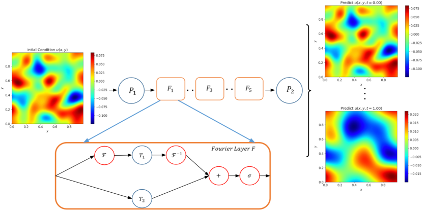
Figure 1: Neural network architecture The top panel shows the architecture of our neural operators, whereas the inset in the bottom panel shows the structure of one of the five Fourier layers, $\{F_{1},...,F_{5}\}$, we use in our PINOs. The top left panel shows the data we feed into our models, labelled as “Initial Condition $u(x,y)$”. This input data are initially lifted into a higher dimension representation by the neural network, $P_{1}$. Thereafter, we apply a series of updates that consist of non-local integral operators and nonlinear activation functions, $\sigma$, shown in the inset labelled as “Fourier Layer F”. Eventually, the neural network $P_{2}$ projects back the updates, producing the output shown on the right panels, which describe the time evolution of the system. In the inset, $T_{1}$ represents a linear transform, $T_{2}$ a local linear transform, $\sigma$ a nonlinear activation function. $\mathcal{F}$ and $\mathcal{F}^{-1}$ stand for Fourier transform and inverse Fourier transform, respectively.

II Modeling physics with artificial neural networks

II.1 Physics informed neural networks

Physics informed neural networks (PINNs) provide a method of using known physical laws to predict the results of various physical systems at high accuracy [25, 26, 27, 28, 29]. These methods estimate the results for a given physical system consisting of a PDE, initial conditions (ICs), and boundary conditions (BCs) by minimizing constraints in the loss function. PINNs utilize the automatic differentiation of deep learning frameworks to compute the derivatives of the PDE to compute the residual error. Despite the success of PINNs, their inability to produce results for different initial conditions prevents them from being useful surrogate models.

II.2 Neural operators

Neural operators use neural networks to learn operators rather than single physical systems. In our case, PDEs are the operator these networks try to learn. Specifically, we provide neural operators with input fields $\mathcal{A}$ that are composed of coordinates and relevant data such as coefficient fields, ICs, and BCs. Neural operators then output the solutions of that operator at those coordinates which we will denote as $\mathcal{U}$. We can mathematically represent the neural operator $\mathcal{G}_{\theta}$ as a mapping between the input fields $\mathcal{A}$ and the output fields $\mathcal{U}$ as

$$\mathcal{G}_{\theta}:\mathcal{A}\rightarrow\mathcal{U}$$ (1)

where $\theta$ are the weights of the neural operator [30].

There are various types of neural operators that have been studied in recent works such as DeepONets, physics informed DeepONets, low-rank neural operators (LNO), graph neural operators (GNO), multipole graph neural operators (MGNO), Fourier neural operators (FNO), and physics informed neural operators [31, 32, 33, 34, 35, 30, 24]. These networks have all illustrated their ability to reproduce the results of operators much faster than computing with the operator directly. For a more detailed look at neural operators, we refer the reader to [30], which provides rigorous definitions of neural operators and examines a large number of different neural operators.

II.3 Physics informed neural operators (PINOs)

PINOs are a variation of neural operators that incorporate knowledge of physical laws into their loss functions [24]. PINOs have been shown to reproduce the results of operators with remarkable accuracy. They employ the FNO architecture which applies a fast Fourier transform (FFT) to the data and applies its fully connected layers in Fourier space before performing an inverse FFT back to real space [35]. Moreover, this architecture has demonstrated the ability to perform zero-shot super-resolution, predicting on higher resolution data having only seen low resolution data [35, 30]. Figure 1 illustrates the FNO architecture that we use in this study.

PINOs improve upon the FNO architecture by adding physics information such as PDEs, ICs, BCs, and other conservation laws. By including the violation of such laws into the loss function, the network can learn these laws in addition to the data. Rather than using automatic differentiation, these networks use Fourier derivatives to compute the derivatives for the PDE constraints as automatic differentiation is very memory intensive for this type of architecture. This physics knowledge enables the network to learn operators faster and with less training data.

III Methods

Here we describe the approach we followed to design, train, validate and test our PINOs, and then how we quantified their accuracy by comparing our predictions with actual numerical solutions of PDEs we consider in this study.

III.1 Initial data

The first step in this process was to generate initial data that matches the boundary conditions of the problem. This was done using the Gaussian random fields (GRF) method in a similar fashion to [24] where the kernel was transformed into Fourier space to match our periodic boundary conditions. We employed a general Matern kernel, but discovered that the PINOs performed better when the smoothness parameter was set to infinity. In this limit, this Matern kernel becomes the radial basis function kernel (RBF) as used in [31] defined as $k_{l}\left(x_{1},x_{2}\right)=\exp\left(-\left\|x_{1}-x_{2}\right\|^{2}/2l^{2}\right)$, where $l$ is the length scale of typical spatial deviations in the data. For this work, we set $l=0.1$ for all cases to provide features at our desired spatial scale except when explicitly stated otherwise. A number of these random fields were produced for each of the test problems described Section IV.

During this work, we found that the magnitude of the training data affected the results of the training even in linear problems. In particular, the models seem to have difficulty with higher magnitude initial data, especially when the data had a magnitude greater than 1. We found that by reducing the magnitude of the initial data, we could improve our results. We believe this is attributed to the highly nonlinear nature of the neural network model. Other neural network models also experience similar effects and therefore normalize their data to improve performance. Thus, we were careful in selecting the magnitude of our input fields during this study.

III.2 Boundary conditions

For our boundary conditions, we used periodic boundary conditions in all cases. This boundary condition is good for problems with significant symmetry over long length scales or for cases where the boundary is sufficiently far from the region of interest. We are particularly focused on the latter case where the boundary condition does not significantly impact the problem. Moreover, the neural network architecture implements periodic boundary conditions by default via FFTs. This periodicity of a certain dimension can be removed by zero padding for said dimension before feeding it to the neural network. We employed this padding in the time dimension with a length of $l_{pad}=5$ for all cases except the 1D wave equation, which is periodic in time for a time interval of $t=1$.

Although we do not do so in this work, one could also use this technique for PDEs with non-periodic BCs by zero padding the spatial dimensions of the data. We could then add an additional loss term for the BC to the loss in Equation 2 to describe our desired BC. We describe how to model similar terms in more detail in Section III.4.

III.3 Training data generation

To generate training data, we took the random IC fields that we had previously generated and evolved them in space and time. Specifically, we evolve each of these equations in time with RK4 time stepping starting at $t=0$ until $t=1$ with the timestep $\delta t$ varying depending on the problem. To compute spatial derivatives, we employed a finite difference method (FDM) with 4th order central difference for most cases. The lone exception was the inviscid Burgers equation in 2D which required a shock capturing method. Therefore, we employed a finite volume method (FVM) with local Lax-Friedrichs (LLF) fluxes and MP5 reconstruction.

III.4 Training approach

We set up the problem as follows. We are given some space and time coordinates as well as the initial conditions at those coordinates. Our objective is to compute the solution at each given space and time coordinate from the initial data. To train the network to reproduce the simulated results, we employ multiple losses to ensure the network properly reproduces the correct loss. These losses are the data loss $\mathcal{L}_{data}$, the physics loss $\mathcal{L}_{phys}$, and the IC loss $\mathcal{L}_{IC}$. We do not include a loss term for the BC here because the FNO architecture of the PINO assures the desired periodic BCs as long as those dimensions are not padded.

$\mathcal{L}_{data}$ attempts to fit the model predictions directly to the training data. This loss is computed via the relative mean squared error (MSE) between the training data and the network outputs. This relative MSE is computed by dividing the MSE of the predictions by the norm of the true values. For cases with multiple equations where the outputs vary in magnitude such as the linear and nonlinear shallow water equations, care must be taken to ensure that each of those outputs contributes equally to $\mathcal{L}_{data}$. Therefore, we compute the relative MSE for each of the output fields separately before combining them together.

$\mathcal{L}_{phys}$ ensures that the PINO predictions obey known physical laws such as PDEs or more general conservation laws. We define the loss as the MSE between the violation of the physical law and the value of said law if it was perfectly satisfied which is $0$ in most cases. Again, one must be careful in cases like the linear and nonlinear shallow water equations with multiple physical laws whose violations differ significantly in their magnitude. In such cases, compute the physical violations separately and multiply each term by some weight before combining them and computing the MSE of the combined term to obtain $\mathcal{L}_{phys}$.

$\mathcal{L}_{IC}$ allows the PINO to learn how the input initial condition given to the network is the value of the output at that point at $t=0$. Moreover, by minimizing $\mathcal{L}_{IC}$, $\mathcal{L}_{phys}$ more easily converges to the correct solution for cases where the physical law is a PDE. We defined $\mathcal{L}_{IC}$ as the relative MSE between the PINO prediction at $t=0$ and the initial condition fed into the network. There were no cases where the ICs differed significantly in magnitude for the PDEs since for the linear and nonlinear shallow water equations, the velocity fields were taken to be zero at $t=0$ and were not fed into the initial data.

To combine these terms into the total loss $\mathcal{L}_{tot}$, we perform a weighted sum defined as

$$\mathcal{L}_{total} =w_{data}\mathcal{L}_{data}+w_{phys}\mathcal{L}_{phys}+w_{IC}\mathcal{L}_{IC}\,,$$ (2)

where $w_{data}$ is the data weight, $w_{phys}$ is the physics weight, and $w_{IC}$ is the IC weight. We varied these values between different cases and even during the training. Typically, we would set $w_{data}$ to be $5$ or $10$, $w_{phys}$ to be $1$ or $2$, and $w_{IC}$ to be $5$ or $10$.

We emphasize that we select the weights in the loss function through a process of trial and error rather than a sophisticated hyperparameter optimization process. This is typically the case with PINNs as well. If we take some limits, we can understand why this is the case. If $w_{phys}$ is very high, the PINO will try to minimize $\mathcal{L}_{phys}$ at the cost of the other parameters. One solution that satisfies the most PDEs is if the output field is zero for all space and time coordinates. Therefore, we add the initial condition loss $\mathcal{L}_{IC}$ to ensure that $\mathcal{L}_{phys}$ evolves the correct initial data. However, if $\mathcal{L}_{IC}$ is too large, the output field is correct at $t=0$, but it does not evolve with time. Thus, we used a process of trial and error to determine the correct weights.

For the training itself, we used the PyTorch framework [36]. We employed an Adam optimizer with $\beta_{1}=0.9$, $\beta_{2}=0.999$ with an initial learning rate of 0.001. To fine tune the latter training steps, we employed a multistep scheduler to reduce the learning rate at several intervals throughout the training with a gamma value of 0.5. The specific number of epochs and the epoch decay milestones vary between the different test cases. A common setup that was used from several of the 2D cases was to train for 150 epochs and put the scheduler milestones at [25, 50, 75, 100, 125, 150] epochs. To further improve the performance, we would use the checkpoints after 150 epochs of training and retrain again after for this same duration. In between restarting from these checkpoints, we would sometimes modify the weights of the various training losses if we observed some losses were lagging behind the others.

III.5 Model architecture

As noted in II.3, the model uses the FNO architecture that is shown in Figure 1. We used a Gaussian error linear units (GELUs) for our nonlinearity for all cases [37]. We note that for physics informed deep learning, we require the nonlinear activation function to have a non-zero second derivative, ruling some commonly used activation functions such as the rectified linear unit (ReLU) [27].

The FNO architecture can be described by the widths, modes, and number of layers. The widths and modes are given as arrays representing the width and modes for each entry. The size of the array gives the number of layers and each entry corresponds to a different layer. We used 4 layers in all cases. For the 1D cases, we used the $width=[16,24,24,32]$ and $modes=[15,12,9,9]$. For the 2D cases, we used $width=[64,64,64,64]$ and $modes=[8,8,8,8]$.

In addition, the network ends with a fully connected layer. We selected a width of 128 for the fully connected layer for all cases.

III.6 Performance quantification

To quantify the performance, we ran PINO on the test dataset, then calculated the MSE of their predictions with the test data and the MSE of the physics loss that accompanied violations of physical laws. The test dataset is composed of approximately $10\%$ of the simulations produced from the random initial data that was separated from the rest of the data to ensure that the PINO did not train on it.

IV Test Problems

We use PINOs to learn nine different PDEs. We consider the wave equation in 1D and 2D to demonstrate that our methods produce accurate and reliable results. We also present results for the 1D Burgers equation, which was used in [24] to quantify the performance of PINOs to learn PDEs. We then put our methods at work to solve a variety of PDEs with different levels of complexity.

Specifically, many past works including [33, 34, 35, 30, 24] investigating using nonlinear neural operators study only 3 cases, the 1D Burgers equation, 2D Darcy Flow, and the 2D Navier Stokes equations. While these cases provide a good way to compare neural operators to each other, they limited the applicability of neural operators to other problems. Moreover, the aforementioned cases fail to include various physical and numerical phenomena such as shocks, coupled PDEs, and non-constant coefficients. Therefore, we chose a wide array of linear and nonlinear PDEs to evaluate the PINO models and isolate the places where they may have difficulty.

IV.1 Wave Equation 1D

Our first test was the wave equation in 1D with periodic boundary conditions. This is a computationally simple PDE that is second order in time and models a variety of different physics phenomena. The equation for the evolved field $u(x,t)$ takes the form

$$u_{tt}+c^{2}u_{xx} =0,$$ (3)

$$u\left(x,0\right) =u_{0}\left(x\right)\,,$$

$$x\in\left[0,1\right), \ t\in\left[0,1\right]\,,$$

where $c=1$ is the speed of the wave.

IV.2 Wave Equation 2D

We extend the wave equation in 2D with periodic boundary conditions to explore the requirements for adding the additional spatial dimension. The equation for the evolved field $u(x,y,t)$ is given by

$$u_{tt}+c^{2}\left(u_{xx}+u_{yy}\ \right)=0$$ (4)

$$u\left(x,y,0\right)=u_{0}\left(x,y\right)\,,$$

$$x,y\in\left[0,1\right),\ t\in\left[0,1\right]\,,$$

where as before the speed of the wave is set to $c=1$.

IV.3 Wave Equation 2D Non-Constant Coefficients

By adding a spatially variable wave speed, we study the performance of PINOs in problems with non-constant coefficients. This variable wave speed $c(x,y)$ was incorporated into the PINO by treating it as another randomly generated input field. To produce smoother training data, we set the spatial scale $l=0.5$ parameter for the wave speed input field $c(x,y)$, though we still used $l=0.1$ for the initial data. The equation for the evolved field $u(x,y,t)$ is now given by

$$u_{tt}+c(x,y)^{2}\left(u_{xx}+u_{yy}\ \right)=0$$ (5)

$$u\left(x,y,0\right)=u_{0}\left(x,y\right)\,,$$

$$x,y\in\left[0,1\right),\ t\in\left[0,1\right]\,.$$

IV.4 Burgers Equation 1D

The 1D Burgers equation with periodic boundary conditions serves as a nonlinear test case with for a variety of numerical methods. This allowed us to verify that our PINOs can learn and reconstruct nonlinear phenomena. The equation for the field $u(x,y,t)$ is given in conservative form by

$$u_{t}+\partial_{x}\left(u^{2}/2\right) =\nu u_{xx},$$ (6)

$$u(x,0) =u_{0}(x)\,,$$

$$x\in[0,1), \ t\in[0,1]\,,$$

where the viscosity $\nu=0.01$.

IV.5 Burgers Equation 2D Scalar

To verify our model can handle nonlinear phenomena in 2D, we extend the Burgers equation into 2D by assuming the field $u(x,y,t)$ is a scalar. The equations take the form

$$u_{t}+\partial_{x}\left(u^{2}/2\right)+\partial_{y}\left(u^{2}/2\right) =\nu\left(u_{xx}+u_{yy}\right)\,,$$ (7)

$$u(x,y,0) =u_{0}(x,y)\,,$$

$$x,y\in[0,1), \ t\in[0,1]\,,\$$

where the viscosity $\nu=0.01$.

IV.6 Burgers Equation 2D Inviscid

We also looked at cases involving the inviscid Burgers equation in 2D in which we set the viscosity $\nu=0$. This setup is known to produce shocks that can result in numerical instabilities if not handled correctly. We used a finite volume method (FVM) to generate this data to ensure stability in the presence of shocks. In turn, this allowed us to investigate the network’s performance when processing shocks. The equations are given by

$$u_{t}+\partial_{x}\left(u^{2}/2\right)+\partial_{y}\left(u^{2}/2\right) =0\,,$$ (8)

$$x,y\in[0,1), \ t\in[0,1]\,,$$

$$u(x,y,0) =u_{0}(x,y).$$

We observed that the presence of the shock prevented our Fourier derivative method from producing accurate residuals when we included the full equation in our physics loss term. Instead, for our physics loss, we used the conserved quantity,

$$\int_{\Omega}u(x,y,t)\ dx\ dy=\int_{\Omega}u(x,y,0)\ dx\ dy=C\,,$$ (9)

where $C$ is a constant and $\Omega$ is the domain. In other words, we ensured that the total $u$ at every time instance is equal to the total $u$ at $t=0$.

IV.7 Burgers Equation 2D Vector

We then looked at a vectorized form of the 2D Burgers equation with periodic boundary conditions. This allowed us to test how well the model handles the coupled fields $u(x,y,t)$ and $v(x,y,t)$ that parameterize the system. The equations take the form

$$u_{t}+uu_{x}+vu_{y}= \nu\left(u_{xx}+u_{yy}\right)\,,$$ (10)

$$v_{t}+uv_{x}+vv_{y}= \nu\left(v_{xx}+v_{yy}\right)\,,$$ (11)

$$u(x,y,0)=u_{0}(x,y), \ v(x,y,0)=v_{0}(x,y),$$

$$x,y\in[0,1), \ t\in[0,1]$$

where the viscosity $\nu=0.01$. We note that this system of equations does not have a conservative form as there is not a continuity equation in this system.

Although coupled equations might seem like a trivial case, there are actually a number of complexities that arise when changing the number of fields. First, having multiple inputs and outputs results in an expanded parameter space for the PINO. Thus, one would expect the network to require a larger volume of training data to produce accurate results. Moreover, PINOs must solve multiple equations simultaneously in the coupled case. In turn, the models must not only solve for single fields, but also compute the contribution of those fields on the other fields. Therefore, it is important to understand how PINOs can resolve coupled fields in this relatively simple 2D vectorized Burgers equation.

IV.8 Linear Shallow Water Equations 2D

To examine the properties of PINOs with 3 coupled equations, we examined the ability of the networks to reproduce the linear shallow water equations with periodic boundary conditions. We assumed that the height of the perturbed surface $h(x,y,t)$ is initially perturbed, but the initial velocity fields $u(x,y,t)$ and $v(x,y,t)$ are initially zero. These equations can be expressed as

$$\frac{\partial h}{\partial t}+H\left(\frac{\partial u}{\partial x}+\frac{\partial v}{\partial y}\right)=0\,,$$ (12)

$$\frac{\partial u}{\partial t}-fv=-g\frac{\partial h}{\partial x}\,,$$ (13)

$$\frac{\partial v}{\partial t}+fu=-g\frac{\partial h}{\partial y}\,,$$ (14)

$$\textrm{with}\quad h(x,y,0)=h_{0}(x,y),\ u(x,y,0)=0,\ v(x,y,0)=0,\$$

$$x,y\in[0,1),\ t\in[0,1],$$

where the gravitational constant $g=1$, the mean fluid height $H=100$, and we considered two cases for the Coriolis coefficient $f=\{0,1\}$.

The challenge in this case is that we have 3 coupled fields with one of them, the perturbed surface height $h$ having a very different physical meaning than the others. Moreover, $h$ is typically of much larger magnitude than either of the velocity fields. By simplifying to a linear problem, we assess the ability of PINOs to reproduce the results of magnitude varying fields without complicated nonlinear terms. We note that coupled equations with terms of varying magnitude are known to be difficult for traditional PINNs as one needs to carefully weight and normalize the equations.

IV.9 Nonlinear Shallow Water Equations 2D

Finally, we examined the network performance on the nonlinear shallow water equations. We assumed a similar setup as in the linear case where we assumed the total fluid column height $\eta(x,y,t)$, was given by a mean value of $1$ plus some initial perturbation. We again assumed the initial velocity fields $u(x,y,t)$ and $v(x,y,t)$ were zero. These equations are given by

$$\frac{\partial(\eta)}{\partial t}+\frac{\partial(\eta u)}{\partial x}+\frac{\partial(\eta v)}{\partial y} =0\,,$$ (15)

$$\frac{\partial(\eta u)}{\partial t}+\frac{\partial}{\partial x}\left(\eta u^{2}+\frac{1}{2}g\eta^{2}\right)+\frac{\partial(\eta uv)}{\partial y} =\nu\left(u_{xx}+u_{yy}\right)\,,$$ (16)

$$\frac{\partial(\eta v)}{\partial t}+\frac{\partial(\eta uv)}{\partial x}+\frac{\partial}{\partial y}\left(\eta v^{2}+\frac{1}{2}g\eta^{2}\right) =\nu\left(v_{xx}+v_{yy}\right)\,,$$ (17)

$$\textrm{with}\quad\eta(x,y,0)=\eta_{0}(x,y),\ u(x,y,0)=0,\ v(x,y,0)=0,\$$

$$x,y\in[0,1),\ t\in[0,1],$$

where the gravitational coefficient $g=1$ and the viscosity coefficient $\nu=0.002$ to prevent the formation of shocks.

This case combines the difficulty of having 3 coupled fields with complicated nonlinear governing equations. This case provides a very useful and physically interesting benchmark for PINOs as these equations model tsunamis. Moreover, these equations take a similar form to the equations of compressible flow, but without an additional equation for energy that is dependent on the equation of state.

All these different PDEs serve the purpose of establishing the accuracy and reliability of our PINOs, and then explore their application for more interesting scenarios for the 2D Burgers equation, and 2D linear and nonlinear shallow waters equations, which involve several coupled equations.

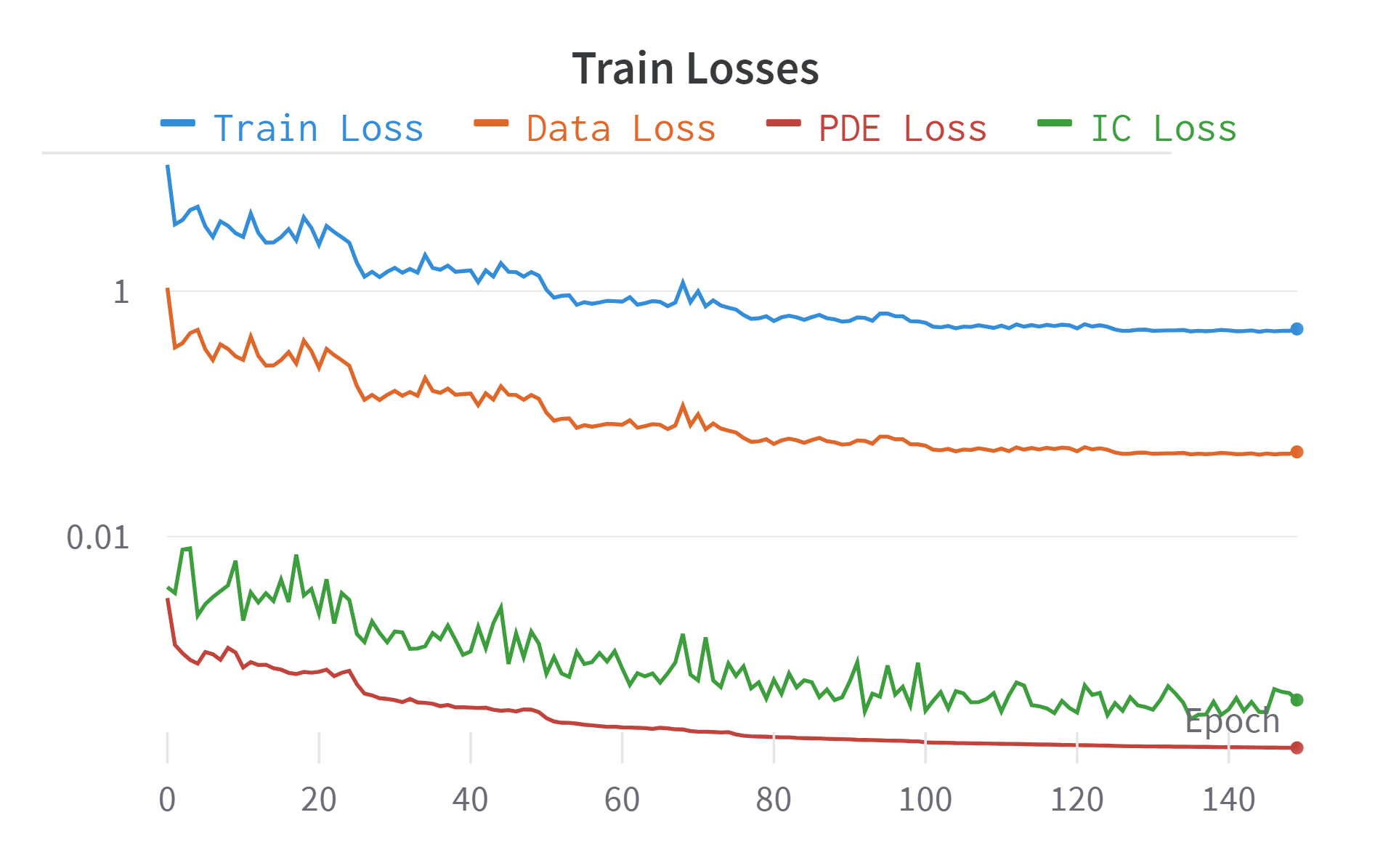
Figure 2: The training loss curves for the first 150 epochs of training for the nonlinear shallow water equations. Here we compare the different losses from the data, PDE, and ICs as well as their weighted total training loss.

Table 1: Summary of PINO results The first column describes the modeled equation. The second and third columns describe the spatial and temporal resolution, respectively. The fifth and sixth columns display the number of training and testing samples used. The final column provides the relative mean squared error (MSE) of our physics informed neural operators on the test set.

Model	Spatial Resolution	Time Steps	Training Samples	Testing Samples	Relative MSE
Wave Equation 1D	128	101	900	100	1.22E-03
Wave Equation 2D	128 $\times$ 128	101	45	25	6.60E-03
Wave Equation 2D Non-Constant Coefficients	128 $\times$ 128	101	175	25	4.86E-02
Burgers Equation 1D	128	101	90	10	6.94E-03
Burgers Equation 2D Scalar	128 $\times$ 128	101	45	25	3.56E-03
Burgers Equation 2D Scalar FNO	128 $\times$ 128	101	45	25	6.29E-03
Burgers Equation 2D Inviscid	128 $\times$ 128	101	90	10	3.56E-02
Burgers Equation 2D Vector	128 $\times$ 128	101	475	25	8.49E-03
Linear Shallow Water Equations 2D f=0	128 $\times$ 128	101	5	25	3.61E-02
Linear Shallow Water Equations 2D f=1	128 $\times$ 128	101	45	25	9.19E-03
Nonlinear Shallow Water Equations 2D	128 $\times$ 128	101	45	25	1.50E-02

V Results

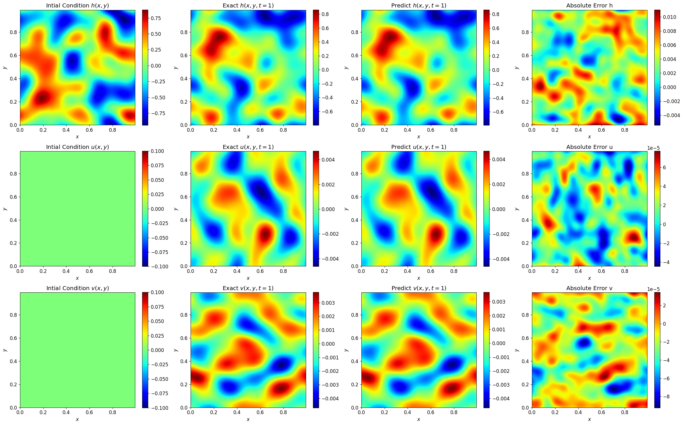
Figure 11: PINO for 2D linear shallow water equation As Figure 10 but now with a Coriolis coefficient $f=1$.

We now quantify the ability of our PINOs to learn the physics described by the PDEs described above. In Figures 3-12 we present qualitative and quantitative results that illustrate the performance of our PINOs. We use two types of quantitative metrics, namely, absolute error (shown in each figure) and mean squared error (summarized in Table 1) between PINO predictions and ground truth simulations. While the figures below provide snapshots of the performance of our PINOs at a given time, $t$, we also provide interactive visualizations of these results at this website. We also provide a tutorial to use our PINOs and reproduce our results in the Data and Learning Hub for Science [38, 39].

Before discussing specific results, we also present the training curves of the nonlinear shallow water equations over its first 150 epochs in Figure 2. Once our PINOs are fully trained, they are computationally efficient. Averaging over 25 test sets, our PINOs produce full simulations within 0.165 seconds for the most computationally intensive case, the nonlinear shallow water equations.

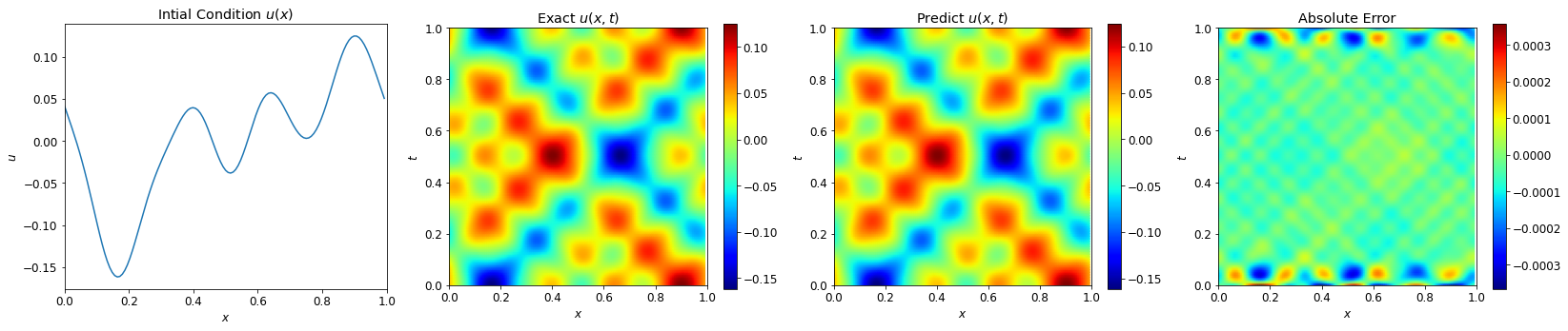
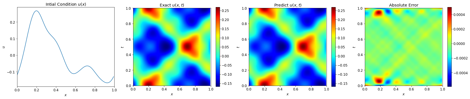
Figure 3: PINO for 1D wave equation Test set initial conditions (left column) fed into our neural networks. The center left column displays the ground truth value of $u_{true}(x,t)$ as produced by our simulations. The center right column shows the value of $u_{pred}(x,t)$ predicted by our PINO. The right column illustrates the error between the PINO predictions and the ground truth, $u_{pred}-u_{true}$.

V.1 Wave Equation 1D Results

Figure 3 shows that our PINO for the 1D wave equation learns and describes the physics of this PDE with remarkable accuracy. These results serve the purpose of validating our methods with a simple PDE. We found that the MSE in this case was $1.22\times 10^{-3}$ on the test dataset. We note that for this case, we experimented with using a very high resolution of $4096$ grid points to generate the training data, but downsampled by a factor of $32$ to a final resolution of $128$ grid points that were fed into the network. This simulates having available less data to reproduce a result than was required to compute it.

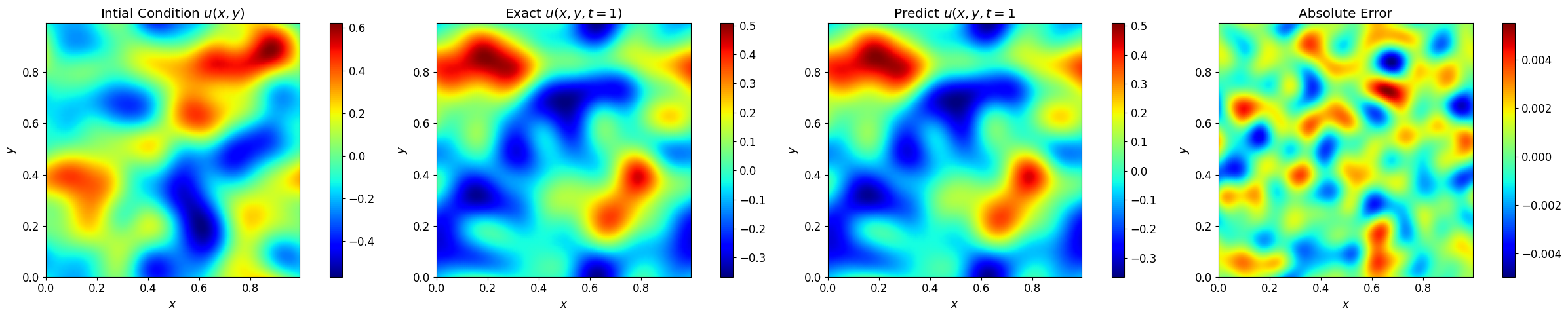
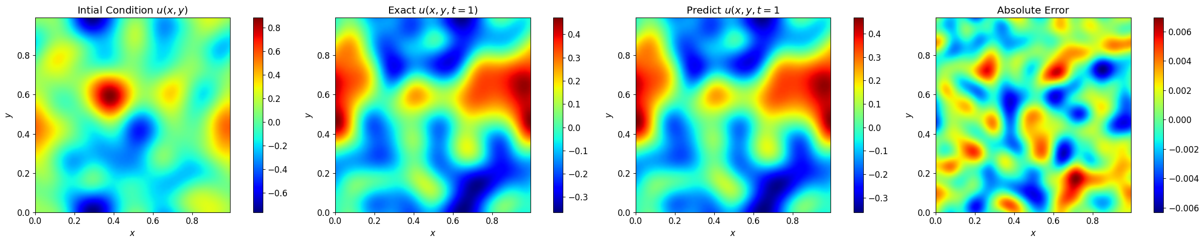
Figure 4: PINO for 2D wave equation As Figure 3, but now in 2D. The left column represents the test set initial conditions that we feed into our PINOs. We evolved the systems until $t=1$ and present ground truth solutions (center left) and PINO predictions (center right). Even after evolving these simulations until the end of the time domain under consideration, our PINOs predict with excellent accuracy the evolution of the system, as shown in the right column which shown at $t=1$, $u_{pred}-u_{true}$.

V.2 Wave Equation 2D Results

Next we consider the 2D wave equation. Figure 4 summarizes our results. As in the 1D scenario, our PINOs have learned the physics of the 2D wave equations with excellent accuracy. Specifically, we found the MSE on the test dataset for this case to be $6.70\times 10^{-3}$.

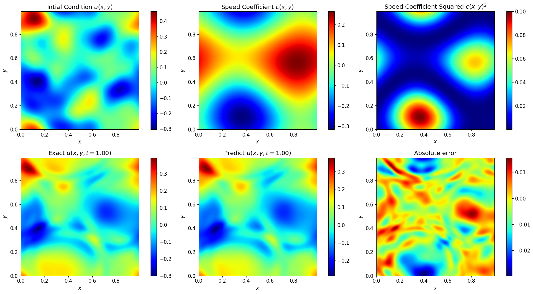
Figure 5: PINO for 2D non-constant coefficients wave equation Similar to Figure 4, but here we have a non-constant wave speed. The top row depicts the input fields into the ANN, which are the initial condition $u$, the wave speed coefficient $c$, and the wave speed coefficient squared $c^{2}$ from left to right respectively. As in the constant coefficient case, we evolved the systems until $t=1$. On the bottom row, we present the values at $t=1$ for the ground truth solutions (left), the PINO predictions (center), the error $u_{pred}-u_{true}$.

V.3 Wave Equation 2D Non-Constant Coefficients Results

Next we consider the variation of the 2D wave equation with non-constant coefficients. Figure 5 illustrates the results for this problem. As this scenario is considerably more difficult than the uniform coefficient wave equation, the PINO performance is slightly worse, with an MSE of on the test dataset of $0.0486$.

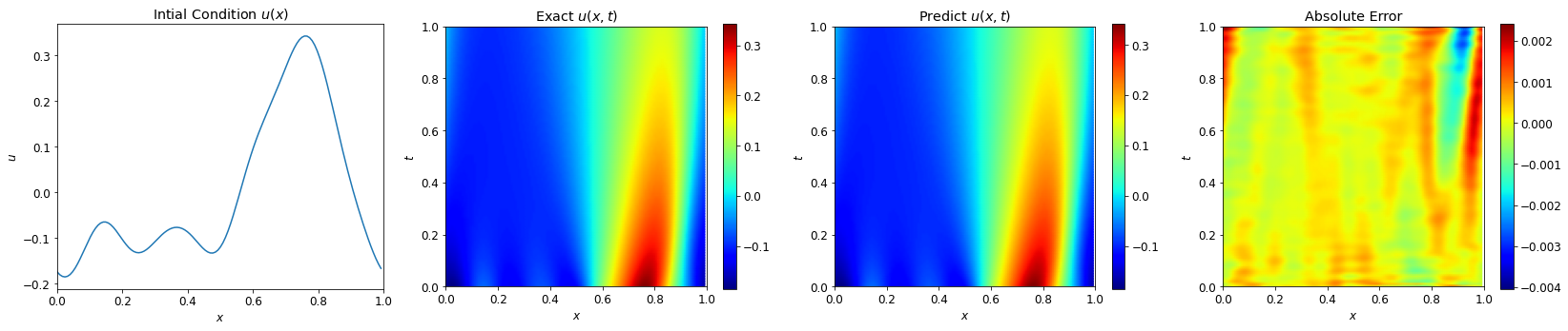
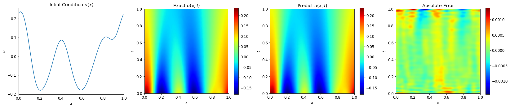
Figure 6: PINO for 1D Burgers equation The left column shows the test set initial conditions fed into our PINOs. The center left column shows the ground truth value, $u_{true}(x,t)$, produced by our simulations. The center right column presents the predicted values $u_{pred}(x,t)$ by our PINOs. The right column shows the discrepancy between PINO and ground truth predictions, $u_{pred}-u_{true}$.

V.4 Burgers Equation 1D Results

We now turn our attention to the Burgers equation, and begin this analysis with a simple and illustrative case, namely the 1D Burgers equation, shown in Figure 6. These results show that our PINOs have accurately learned the physics described by this PDE with an excellent level of accuracy. Quantitatively, the MSE on the test dataset was $6.94\times 10^{-3}$. These results furnish evidence that our methods can reproduce results published elsewhere in the literature [24].

We now turn our attention to several 2D Burgers equations that, to the best of our knowledge, have not been explored previously in the literature.

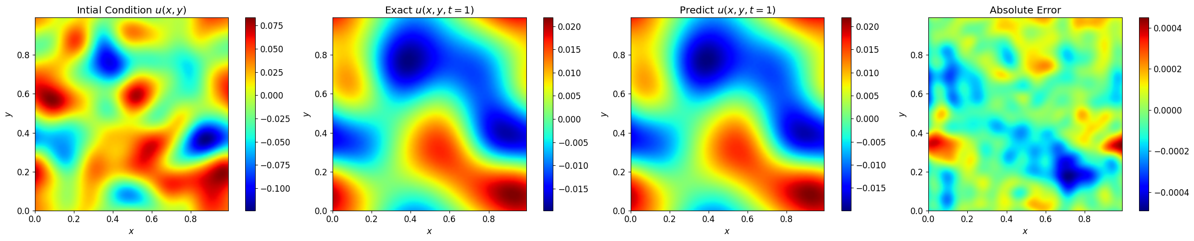
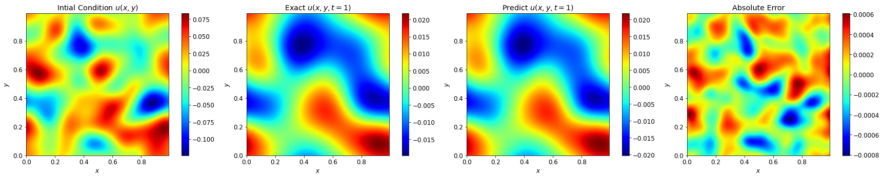
Figure 7: PINO and FNO for 2D scalar Burgers equation Displays the results of the PINO and FNO models for this equation. The left column shows a sample of test set initial conditions fed into our models. The center left column displays the ground truth value, $u_{true}(x,y)$, of our simulations once they have evolved up to $t=1$. The center right column shows model predictions for this PDE at $t=1$. We have selected this time to quantify the accuracy of our model once the system has evolved sufficient time to accumulate errors. The right column illustrates the discrepancy between model predictions and the ground truth, $u_{pred}-u_{true}$, at $t=1$. The top row shows the results for the PINO and the bottom row shows the results for the FNO.

V.5 Burgers Equation 2D Scalar Results

This PDE is given by Equation (7). As shown in Figure 7 our PINOs can learn and describe the physics of this PDE accurately. Note that we present results for this PDE once the system has been evolved throughout the time domain under consideration, i.e., $t\in[0,1]$. By presenting results at $t=1$ we gain a good understanding of the actual performance of our PINOs once they have evolved in time and accumulated numerical errors that may depart from ground truth values. For this case, we compared the results to a FNO which was trained with the same architecture, but without a physics informed loss component. In Figure 7 we present the results of the PINO and the FNO for the same initial condition. We found that the MSE for the full test dataset was $3.56\times 10^{-3}$. for the PINO and was $6.29\times 10^{-3}$ for the FNO.

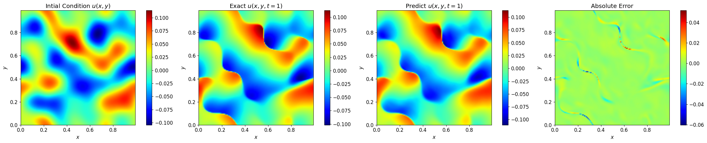
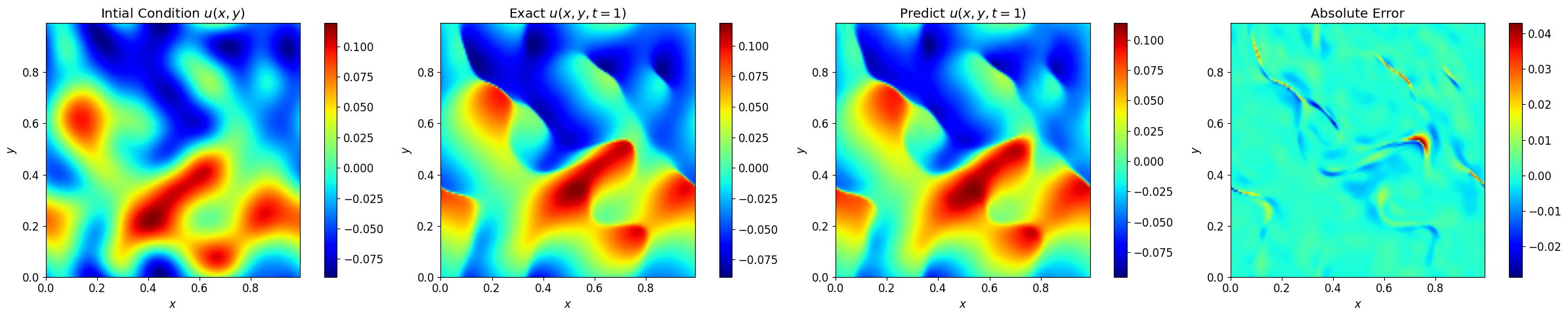
Figure 8: PINO for 2D inviscid Burgers equation As Figure 7 but now in the inviscid case given by Equation 8.

V.6 Burgers Equation 2D Inviscid Results

This PDE is given by Equation 8. As we mentioned before, shocks are a common occurrence for this PDEs, and may lead to numerical instabilities if we do not use shock capturing schemes. We have quantified the ability of our PINOs to handle shocks. We found the PINO to have an MSE of $0.0356$ on the test dataset. In Figure 8 we notice that our PINOs are able to describe the physics of this PDE with excellent accuracy. However, we observe a significant discrepancy between ground truth and AI predictions right at the regions where shocks occur. These findings indicate that further work is needed to better handle PDEs that involve shocks. This is a specific area of work that we will pursue in the future.

Specifically, such work would look at improvements to the way the model and loss function handle discontinuities in the data. For example, Fourier transforms, which are employed in the neural network and to represent derivatives in the loss function, are known to be highly sensitive to discontinuities. Thus, potential improvements may encompass the use of Galerkin neural networks [40] to better handle discontinuities, and loss functions that incorporate particle number conservation. These improvements should be considered in future work.

V.7 Burgers Equation 2D Vector Results

This is the most complex PDE of the Burgers family we consider in this study, see Equations (10) and (11). The novel feature of this PDE is that we now need to treat two different fields $(u,v)$. In Figure 9 we present a sample result from the test dataset, which demonstrate that our PINOs have learned the physics of this PDE and describe it with remarkable precision even after we have evolved this system until the end of the time domain under consideration. Quantitatively, we achieved an MSE of $8.49\times 10^{-3}$ on the test dataset.

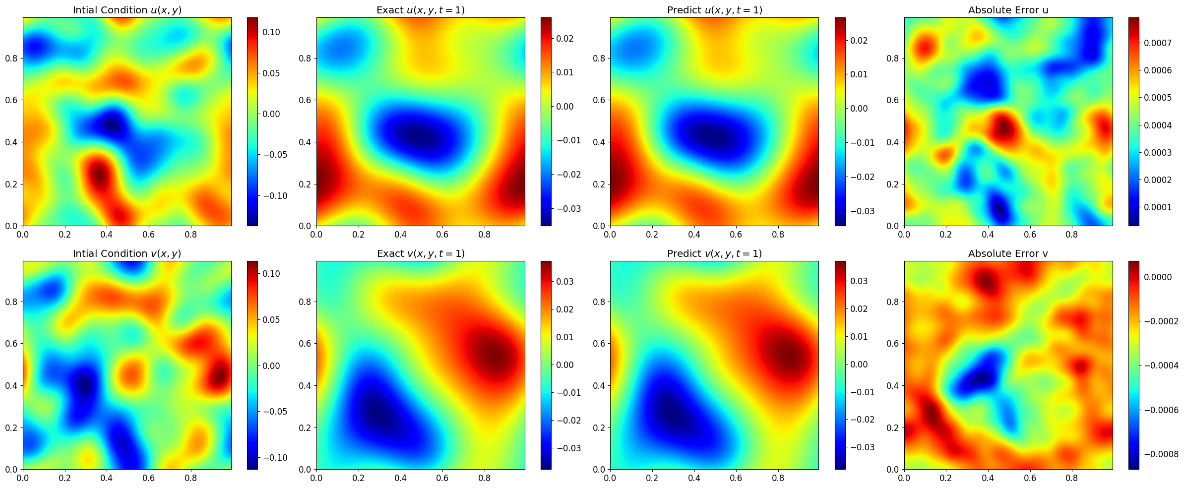
Figure 9: PINO for 2D vector Burgers equation The top and bottom rows show the $u$ and $v$ fields, respectively. The left column shows test set initial conditions for $(u,v)$. The center left column shows ground truth values for the $(u,v)$ fields once this PDE has been evolved up to $t=1$. The center right column shows PINO results for the $(u,v)$ fields at $t=1$. The right column show the discrepancy between PINO and ground truth values at $t=1$.

These results complete our analysis for a variety of PDEs that involve the Burgers equation, and indicate that for various levels of complexity and initial conditions our PINOs are capable of learning and describing the physics of these PDEs with excellent accuracy. We have also realized that we need to further develop these methods for PDEs that involve shocks. We are keenly interested in this particular case, and will explore in future work.

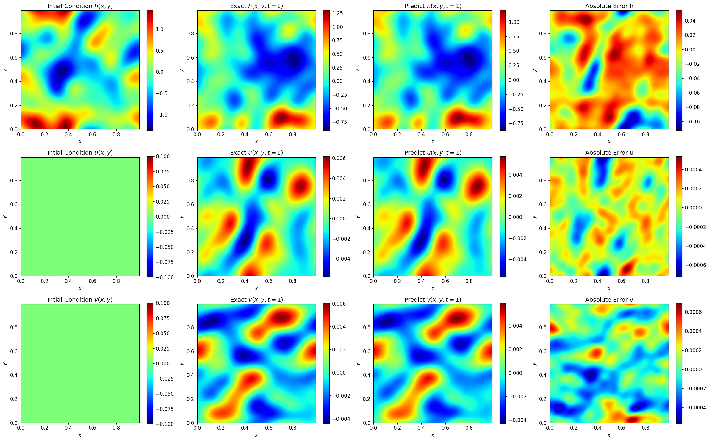
Figure 10: PINO for 2D linear shallow water equation Assuming a system with a Coriolis coefficient $f=0$, we show the $h$, $u$, and $v$ fields in the top, middle, and bottom rows, respectively. The left column shows the initial condition provided to the network. The center left column displays the ground truth value at $t=1$ as produced by the simulation. The center right column shows the value of prediction at $t=1$ predicted by our PINO. The right column indicates the discrepancy between PINO predictions and the ground truth at $t=1$.

V.8 Linear Shallow Water Equations 2D Results

Another original result in this study is the use of PINOs to learn the physics of 3 coupled PDE equations. The first case under consideration is the 2D linear shallow water equation given by Equations (12)-(14). In this case we now consider the height of the perturbed surface, $h$, and the fields $(u,v)$. Figures 10 and 11 present results assuming two Coriolis coefficient $f=\{0,1\}$, respectively. The discrepancy between PINO predictions and ground truth values in the figures is very small, which furnishes strong evidence for the adequacy of PINOs to learn the physics of this PDE Highlights of these results include:

• $\mathbf{f=0}$ case: We only required 5 training samples to produce PINOs that exhibit optimal performance. In this case, the MSE on the test dataset was $0.0361$. This illustrates the ability of our PINOs to generalize from very sparse training data.

• $\mathbf{f=1}$ case: We increased the number of training samples to 45, which is comparable to some of the other 2D cases. The MSE on the test dataset was calculated to be $9.19\times 10^{-3}$.

These results provide a glimpse of the capabilities of PINOs to learn the physics of these linear, coupled PDEs. We have extensively tested these equations and found that they are robust to a broad range of initial data. These results provided enough motivation to explore the use of PINOs for a more challenging set of coupled PDEs, namely, the 2D nonlinear shallow water equations that we discuss next.

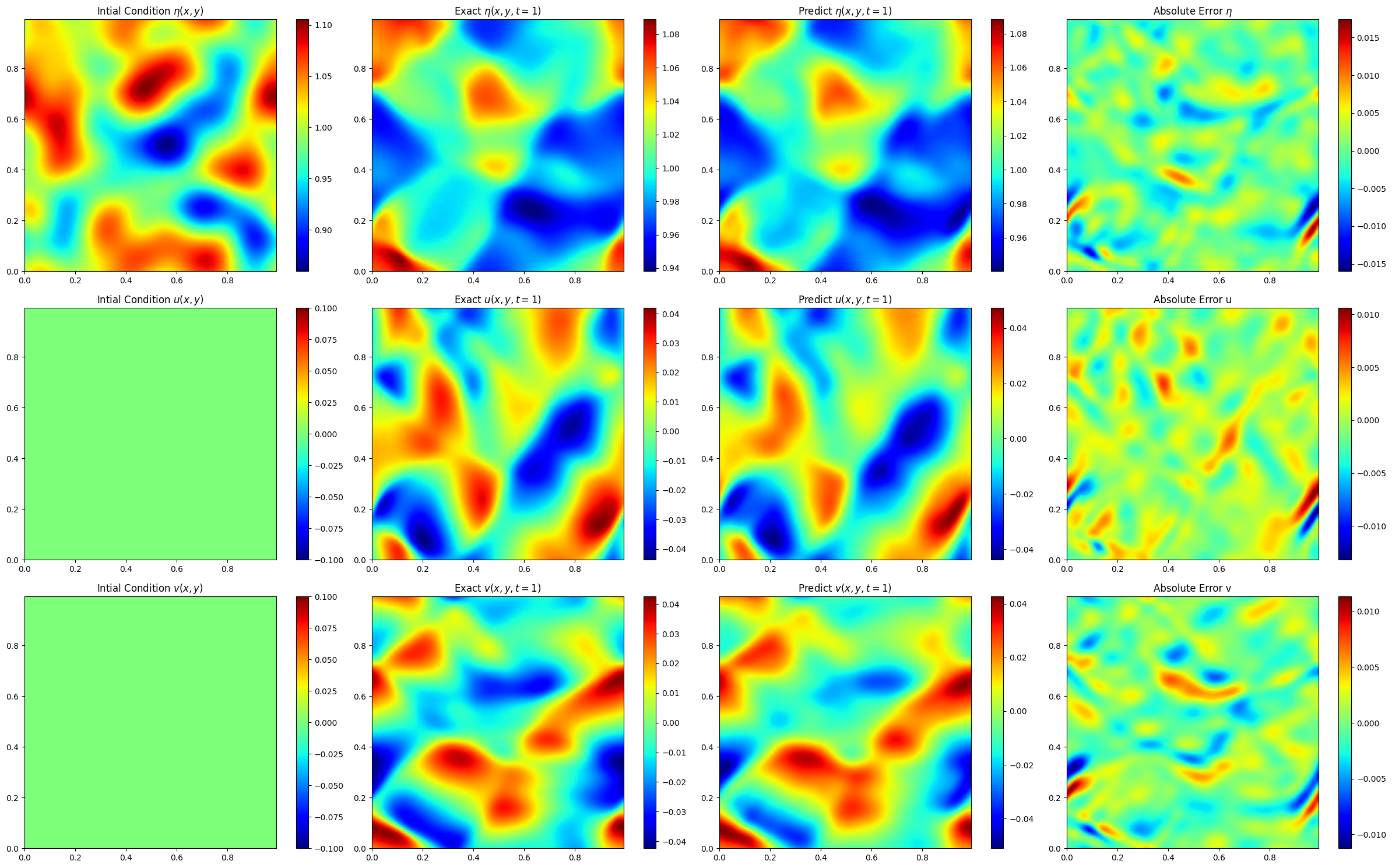
Figure 12: PINO for 2D nonlinear shallow water equation The $(\eta,u,v)$ fields are shown in the top, middle, and bottom rows, respectively. The left column presents the test set initial condition that is fed into our network. The center left column displays the ground truth value at $t=1$ as produced by our simulations. The center right column shows the value of prediction at $t=1$ predicted by the PINO. The right column illustrates the discrepancy between the PINO predictions and the ground truth at $t=1$.

V.9 Nonlinear Shallow Water Equations 2D Results

The final original contribution of this study is the use of PINOs to learn the physics of the 2D nonlinear shallow water equation, given by Equations (15)- (17). Even though this PDE is significantly more complex than its linear counterpart, we notice in Figure 12 that our PINOs learn the physics described by the fields $(\eta,u,v)$ with remarkable accuracy. We found the MSE for the test dataset of this case to be 0.0150

Finally, we provide an additional metric to quantify the overall performance of all the PDEs we have used in this study in Table 1. These results indicate that our PINOs provide state-of-the-art results to model simple PDEs (1D wave equation & 1D Burgers equations), and excellent performance for a variety of PDEs that are solved for the first time in the literature with physics informed neural operators.

VI Conclusions

We have introduced an end-to-end framework to learn PDEs that range from simple equations that serve the purpose of testing our methods (1D wave equation & 1D Burgers equation) to increasingly more complex equations (2D scalar, 2D inviscid and 2D vector Burgers equation), and coupled PDEs that are solved with PINOs for the first time in the literature (2D linear & nonlinear shallow waters equations). The methods we introduce in this study provide the flexibility to produce initial data to test the robustness and applicability of AI surrogates for a broad range of physically motivated scenarios. We provide scientific visualizations of our results through an interactive website. We also release our PINOs and scientific software through the Data and Learning Hub for Science so that AI practitioners may download, use and further develop our neural networks. In addition to this Data and Learning Hub for Science implementation, we release the source code used in this paper.

Future work may focus on the extension of these PINOs to high-dimensional PDEs that are relevant for the modeling of complex phenomena that demand subgrid scale precision, and which typically lead to computationally expensive simulations. We will also focus on developing methods that handle shocks effectively, since these phenomena are common in fluid dynamics and relativistic astrophysics, to mention a few. We will also continue our research program combining scientific visualization and accelerated computing to gain insights about what PINOs learn from data, and how this information may be used to enhance their performance when applied to experimental datasets [41, 42, 43].

It is our expectation that our AI surrogates may be used to replace computationally demanding numerical methods to learn PDEs in scientific software used to model multi-scale and multi-physics phenomena—e.g., numerical relativity simulations of gravitational wave sources, weather forecasting, etc.,—and eventually provide data-driven and physics informed solutions that more accurately describe and identify novel features and patterns in experimental data.

References

- Geroch [1996] R. P. Geroch, Partial differential equations of physics, in 46th Scottish Universities Summer School in Physics: General Relativity (1996) arXiv:gr-qc/9602055
- Press et al. [2007] W. H. Press, S. A. Teukolsky, W. T. Vetterling, and B. P. Flannery, Numerical Recipes 3rd Edition: The Art of Scientific Computing, 3rd ed. (Cambridge University Press, USA, 2007)
- Radice [2020] D. Radice, Binary Neutron Star Merger Simulations with a Calibrated Turbulence Model, Symmetry 12, 1249 (2020), arXiv:2005.09002 [astro-ph.HE]
- Radice et al. [2021] D. Radice, S. Bernuzzi, A. Perego, and R. Haas, A New Moment-Based General-Relativistic Neutrino-Radiation Transport Code: Methods and First Applications to Neutron Star Mergers, arXiv e-prints , arXiv:2111.14858 (2021), arXiv:2111.14858 [astro-ph.HE]
- Foucart [2020] F. Foucart, A brief overview of black hole-neutron star mergers, Frontiers in Astronomy and Space Sciences 7, 10.3389/fspas.2020.00046 (2020)
- Schalkwijk et al. [2015] J. Schalkwijk, H. J. J. Jonker, A. P. Siebesma, and E. V. Meijgaard, Weather forecasting using gpu-based large-eddy simulations, Bulletin of the American Meteorological Society 96, 715 (2015)
- Erba et al. [2017] A. Erba, J. Baima, I. Bush, R. Orlando, and R. Dovesi, Large-scale condensed matter dft simulations: Performance and capabilities of the crystal code, Journal of Chemical Theory and Computation 13, 5019 (2017), pMID: 28873313, https://doi.org/10.1021/acs.jctc.7b00687
- Asch et al. [2018] M. Asch, T. Moore, R. Badia, M. Beck, P. Beckman, T. Bidot, F. Bodin, F. Cappello, A. Choudhary, B. de Supinski, E. Deelman, J. Dongarra, A. Dubey, G. Fox, H. Fu, S. Girona, W. Gropp, M. Heroux, Y. Ishikawa, K. Keahey, D. Keyes, W. Kramer, J.-F. Lavignon, Y. Lu, S. Matsuoka, B. Mohr, D. Reed, S. Requena, J. Saltz, T. Schulthess, R. Stevens, M. Swany, A. Szalay, W. Tang, G. Varoquaux, J.-P. Vilotte, R. Wisniewski, Z. Xu, and I. Zacharov, Big data and extreme-scale computing: Pathways to convergence-toward a shaping strategy for a future software and data ecosystem for scientific inquiry, The International Journal of High Performance Computing Applications 32, 435 (2018)
- Gropp et al. [2020] W. Gropp, S. Banerjee, and I. Foster, Infrastructure for Artificial Intelligence, Quantum and High Performance Computing, arXiv e-prints , arXiv:2012.09303 (2020), arXiv:2012.09303 [cs.CY]
- Huerta et al. [2020] E. A. Huerta, A. Khan, E. Davis, C. Bushell, W. D. Gropp, D. S. Katz, V. Kindratenko, S. Koric, W. T. C. Kramer, B. McGinty, K. McHenry, and A. Saxton, Convergence of Artificial Intelligence and High Performance Computing on NSF-supported Cyberinfrastructure, Journal of Big Data 7, 88 (2020), arXiv:2003.08394 [physics.comp-ph]
- Taher [2009] M. Taher, Accelerating scientific applications using gpu’s, in 2009 4th International Design and Test Workshop (IDT) (2009) pp. 1–6
- Rodrigues et al. [2008] C. I. Rodrigues, D. J. Hardy, J. E. Stone, K. Schulten, and W.-M. W. Hwu, Gpu acceleration of cutoff pair potentials for molecular modeling applications, in Proceedings of the 5th Conference on Computing Frontiers, CF ’08 (Association for Computing Machinery, New York, NY, USA, 2008) p. 273–282
- Wysocki et al. [2019] D. Wysocki, R. O’Shaughnessy, J. Lange, and Y.-L. L. Fang, Accelerating parameter inference with graphics processing units, Phys. Rev. D 99, 084026 (2019), arXiv:1902.04934 [astro-ph.IM]
- Graff et al. [2012] P. Graff, F. Feroz, M. P. Hobson, and A. Lasenby, BAMBI: blind accelerated multimodal Bayesian inference, MNRAS 421, 169 (2012), arXiv:1110.2997 [astro-ph.IM]
- Rosofsky and Huerta [2020] S. G. Rosofsky and E. A. Huerta, Artificial neural network subgrid models of 2D compressible magnetohydrodynamic turbulence, Phys. Rev. D 101, 084024 (2020), arXiv:1912.11073 [physics.comp-ph]
- Huerta and Zhao [2020] E. A. Huerta and Z. Zhao, Advances in machine and deep learning for modeling and real-time detection of multi-messenger sources, in Handbook of Gravitational Wave Astronomy, edited by C. Bambi, S. Katsanevas, and K. D. Kokkotas (Springer Singapore, Singapore, 2020) pp. 1–27
- Cuoco et al. [2021] E. Cuoco, J. Powell, M. Cavaglià, K. Ackley, M. Bejger, C. Chatterjee, M. Coughlin, S. Coughlin, P. Easter, R. Essick, H. Gabbard, T. Gebhard, S. Ghosh, L. Haegel, A. Iess, D. Keitel, Z. Marka, S. Marka, F. Morawski, T. Nguyen, R. Ormiston, M. Puerrer, M. Razzano, K. Staats, G. Vajente, and D. Williams, Enhancing Gravitational-Wave Science with Machine Learning, Mach. Learn. Sci. Tech. 2, 011002 (2021)
- Huerta et al. [2021] E. A. Huerta, A. Khan, X. Huang, M. Tian, M. Levental, R. Chard, W. Wei, M. Heflin, D. S. Katz, V. Kindratenko, D. Mu, B. Blaiszik, and I. Foster, Accelerated, scalable and reproducible AI-driven gravitational wave detection, Nature Astronomy 5, 1062 (2021), arXiv:2012.08545 [gr-qc]
- Huerta et al. [2019] E. A. Huerta, G. Allen, I. Andreoni, J. M. Antelis, E. Bachelet, G. B. Berriman, F. B. Bianco, R. Biswas, M. Carrasco Kind, K. Chard, M. Cho, P. S. Cowperthwaite, Z. B. Etienne, M. Fishbach, F. Forster, D. George, T. Gibbs, M. Graham, W. Gropp, R. Gruendl, A. Gupta, R. Haas, S. Habib, E. Jennings, M. W. G. Johnson, E. Katsavounidis, D. S. Katz, A. Khan, V. Kindratenko, W. T. C. Kramer, X. Liu, A. Mahabal, Z. Marka, K. McHenry, J. M. Miller, C. Moreno, M. S. Neubauer, S. Oberlin, A. R. Olivas, D. Petravick, A. Rebei, S. Rosofsky, M. Ruiz, A. Saxton, B. F. Schutz, A. Schwing, E. Seidel, S. L. Shapiro, H. Shen, Y. Shen, L. P. Singer, B. M. Sipocz, L. Sun, J. Towns, A. Tsokaros, W. Wei, J. Wells, T. J. Williams, J. Xiong, and Z. Zhao, Enabling real-time multi-messenger astrophysics discoveries with deep learning, Nature Reviews Physics 1, 600 (2019), arXiv:1911.11779 [gr-qc]
- Khan et al. [2022] A. Khan, E. A. Huerta, and H. Zheng, Interpretable AI forecasting for numerical relativity waveforms of quasicircular, spinning, nonprecessing binary black hole mergers, Phys. Rev. D 105, 024024 (2022), arXiv:2110.06968 [gr-qc]
- Chaturvedi et al. [2022] P. Chaturvedi, A. Khan, M. Tian, E. A. Huerta, and H. Zheng, Inference-Optimized AI and High Performance Computing for Gravitational Wave Detection at Scale, Front. Artif. Intell. 5, 828672 (2022), arXiv:2201.11133 [gr-qc]
- Wilkinson et al. [2016] M. Wilkinson, M. Dumontier, I. J. Aalbersberg, G. Appleton, M. Axton, A. Baak, N. Blomberg, J.-W. Boiten, L. O. Bonino da Silva Santos, P. Bourne, J. Bouwman, A. Brookes, T. Clark, M. Crosas, I. Dillo, O. Dumon, S. Edmunds, C. Evelo, R. Finkers, and B. Mons, The fair guiding principles for scientific data management and stewardship, Scientific Data 3 (2016)
- Chen et al. [2022] Y. Chen, E. A. Huerta, J. Duarte, P. Harris, D. S. Katz, M. S. Neubauer, D. Diaz, F. Mokhtar, R. Kansal, S. Eon Park, V. V. Kindratenko, Z. Zhao, and R. Rusack, A FAIR and AI-ready Higgs boson decay dataset, Scientific Data 9, 31 (2022), arXiv:2108.02214 [hep-ex]
- Li et al. [2021] Z. Li, H. Zheng, N. Kovachki, D. Jin, H. Chen, B. Liu, K. Azizzadenesheli, and A. Anandkumar, Physics-Informed Neural Operator for Learning Partial Differential Equations, arXiv e-prints , arXiv:2111.03794 (2021), arXiv:2111.03794 [cs.LG]
- Raissi et al. [2017a] M. Raissi, P. Perdikaris, and G. E. Karniadakis, Physics informed deep learning (part i): Data-driven solutions of nonlinear partial differential equations (2017a), arXiv:1711.10561 [cs.AI]
- Raissi et al. [2017b] M. Raissi, P. Perdikaris, and G. E. Karniadakis, Physics informed deep learning (part ii): Data-driven discovery of nonlinear partial differential equations (2017b), arXiv:1711.10566 [cs.AI]
- Raissi et al. [2019] M. Raissi, P. Perdikaris, and G. Karniadakis, Physics-informed neural networks: A deep learning framework for solving forward and inverse problems involving nonlinear partial differential equations, Journal of Computational Physics 378, 686 (2019)
- Pang et al. [2019] G. Pang, L. Lu, and G. E. Karniadakis, fpinns: Fractional physics-informed neural networks, SIAM Journal on Scientific Computing 41, A2603 (2019), https://doi.org/10.1137/18M1229845
- Lu et al. [2021a] L. Lu, X. Meng, Z. Mao, and G. E. Karniadakis, DeepXDE: A deep learning library for solving differential equations, SIAM Review 63, 208 (2021a)
- Kovachki et al. [2021] N. Kovachki, Z. Li, B. Liu, K. Azizzadenesheli, K. Bhattacharya, A. Stuart, and A. Anandkumar, Neural Operator: Learning Maps Between Function Spaces, arXiv e-prints , arXiv:2108.08481 (2021), arXiv:2108.08481 [cs.LG]
- Lu et al. [2021b] L. Lu, P. Jin, G. Pang, Z. Zhang, and G. E. Karniadakis, Learning nonlinear operators via deeponet based on the universal approximation theorem of operators, Nature Machine Intelligence 3, 218–229 (2021b)
- Wang et al. [2021] S. Wang, H. Wang, and P. Perdikaris, Learning the solution operator of parametric partial differential equations with physics-informed DeepONets, Science Advances 7, eabi8605 (2021)
- Li et al. [2020a] Z. Li, N. Kovachki, K. Azizzadenesheli, B. Liu, K. Bhattacharya, A. Stuart, and A. Anandkumar, Neural operator: Graph kernel network for partial differential equations (2020a), arXiv:2003.03485 [cs.LG]
- Li et al. [2020b] Z. Li, N. B. Kovachki, K. Azizzadenesheli, B. Liu, K. Bhattacharya, A. M. Stuart, and A. Anandkumar, Multipole graph neural operator for parametric partial differential equations, CoRR abs/2006.09535 (2020b), 2006.09535
- Li et al. [2020c] Z. Li, N. Kovachki, K. Azizzadenesheli, B. Liu, K. Bhattacharya, A. Stuart, and A. Anandkumar, Fourier neural operator for parametric partial differential equations (2020c), arXiv:2010.08895 [cs.LG]
- Paszke et al. [2019] A. Paszke, S. Gross, F. Massa, A. Lerer, J. Bradbury, G. Chanan, T. Killeen, Z. Lin, N. Gimelshein, L. Antiga, et al., Pytorch: An imperative style, high-performance deep learning library, Advances in neural information processing systems 32 (2019)
- Hendrycks and Gimpel [2016] D. Hendrycks and K. Gimpel, Gaussian error linear units (gelus) (2016), arXiv:1606.08415 [cs.LG]
- Chard et al. [2019] R. Chard, Z. Li, K. Chard, L. Ward, Y. Babuji, A. Woodard, S. Tuecke, B. Blaiszik, M. J. Franklin, and I. Foster, Dlhub: Model and data serving for science, 2019 IEEE International Parallel and Distributed Processing Symposium (IPDPS) 10.1109/ipdps.2019.00038 (2019)
- Blaiszik et al. [2019] B. Blaiszik, L. Ward, M. Schwarting, J. Gaff, R. Chard, D. Pike, K. Chard, and I. Foster, A data ecosystem to support machine learning in materials science, MRS Communications 9, 1125 (2019)
- Ainsworth and Dong [2021] M. Ainsworth and J. Dong, Galerkin neural networks: A framework for approximating variational equations with error control, SIAM Journal on Scientific Computing 43, A2474 (2021)
- Doshi-Velez and Kim [2017] F. Doshi-Velez and B. Kim, Towards A Rigorous Science of Interpretable Machine Learning, arXiv e-prints , arXiv:1702.08608 (2017), arXiv:1702.08608 [stat.ML]
- Safarzadeh et al. [2022] M. Safarzadeh, A. Khan, E. A. Huerta, and M. Wattenberg, Interpreting a Machine Learning Model for Detecting Gravitational Waves, arXiv e-prints , arXiv:2202.07399 (2022), arXiv:2202.07399 [gr-qc]
- Carvalho et al. [2019] D. V. Carvalho, E. M. Pereira, and J. S. Cardoso, Machine learning interpretability: A survey on methods and metrics, Electronics 8, 10.3390/electronics8080832 (2019)