- AP
- access point
- BPP
- binomial point process
- BLP
- binomial line process
- BLCP
- binomial line Cox process
- CCDF
- complementary cumulative density function
- CDF
- cumulative density function
- probability density function
- PPP
- Poisson point process
- BS
- base station
- LOS
- line of sight
- SINR
- signal-to-interference-plus-noise ratio
- SNR
- signal to noise ratio
- mm-wave
- millimeter wave
- PV
- Poisson-Voronoi
- LOS
- line-of-sight
- NLOS
- non line-of-sight
- PGFL
- probability generating functional
- PLCP
- Poisson line Cox process
- MBS
- macro base station
- PLT
- Poisson line tessellation
- SBS
- small cell base station
- RAT
- radio access technique
- 5G
- fifth generation
- PLP
- Poisson line process
- UE
- user equipment
Binomial Line Cox Processes: Statistical Characterization and Applications in Wireless Network Analysis
Abstract
The current analysis of wireless networks whose transceivers are confined to streets is largely based on Poissonian models, such as Poisson line processes and Poisson line Cox processes. We demonstrate important scenarios where a model with a finite and deterministic number of streets, termed binomial line process, is more accurate. We characterize the statistical properties of the BLP and the corresponding binomial line Cox process and apply them to analyze the performance of a network whose access points are deployed along the streets of a city. Such a deployment scenario will be typical for 5G and future wireless networks. In order to obtain a fine-grained insight into the network performance, we derive the meta distribution of the signal-to-interference and noise ratio. Accordingly, we investigate the mean local delay in transmission and the density of successful transmission. These metrics, respectively, characterize the latency and coverage performance of the network and are key performance indicators of next-generation wireless systems.
Stochastic geometry, Line processes, Binomial point processes, Cox process, Meta Distributions.
I Introduction
I-A Motivation
††The codes for generating the numerical results of this paper are available for download [1].Line processes are useful statistical tools for studying a variety of engineering problems such as transportation and urban infrastructure planning, wireless communications, and industrial automation scenarios [2, 3]. In the two-dimensional Euclidean plane, a line process, is a random collection of lines whose locations and orientations reside in a parameter space (to be defined shortly) according to a spatial stochastic process. Leveraging a line process, researchers often study doubly-stochastic processes called Cox processes, which are Poisson point processes defined with the line process as their restricting domain [4]. These models are key in deriving insights into engineering and planning questions such as
-
•
How many electric vehicle charging points does a city need to have along the streets?
-
•
From a typical urban home, how far is the nearest bus stop? Accordingly, what should be the density of bus stops in a given city?
-
•
For on-road deployments of wireless small cells as envisaged in 5G and future networks, what would be the cellular coverage performance of a user in the city?
In the context of wireless communications in particular, AT&T plans to deploy compact Ericsson street radio small cells integrated with the street lights to accelerate 5G deployments [5]. Along the same lines, New York City has already deployed such small cells focusing on high-speed connectivity for pedestrian users [6]. Such deployments seamlessly integrate access points in the urban infrastructure to provide ubiquitous connectivity to the users. In this regard, the network coverage of any point in the network for such on-street deployed small cells is a major point of interest for network operators.
I-B Related Work
In the literature, several line processes have been used to study the structure of streets, e.g., the Poisson line process (PLP), the Poisson Voronoi tessellation (PVT), and the Poisson lilypond model [7, 8, 9, 10]. Out of all the candidate line processes, the most popular one for modeling streets, especially in wireless network studies, is the PLP [11, 9]. The statistical properties of the PLP provide significant tractability in developing insights into the engineering problems of interest. For example, in [12], the authors have employed the PLP and Poisson line Cox process (PLCP) for studying on-street deployment of small cell base stations and derived the performance of a pedestrian user in a multi-tier multi radio access technique (RAT) cellular network. Similarly, in [13, 14], the authors have characterized the performance of vehicular networks based on the PLP model for streets and consequently, PLCP for emulating vehicular nodes. However, one major drawback of the PLP is that it fails to accurately take into account some salient features of urban street networks, e.g., finite street lengths, T-junctions, and varying density of streets across a given city.111From an infrastructure planning perspective, the density of the streets is measured in terms of the total street length per unit area. The recent work by Jeyaraj et al. [9] proposed a generalized framework for Cox models to study vehicular networks. The authors significantly improved the accuracy of line process models to account for finite street lengths by considering T-junctions, stick processes, and Poisson lilypond models. However, their work does not consider varying line densities from the perspective of a single city. This is an important aspect of applications such as urban transport networks and wireless deployment planning, in which streets near the city center are denser as compared to the streets in the suburbs. Such characteristics of an urban scenario can only be studied using non-homogeneous line processes which is the focus of this paper.
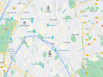
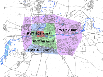
To illustrate this, the street network of Paris is shown in Fig. 1a, where, as we move out of the city center, the street density decreases. More precisely, in [15], researchers have emulated the streets of Lyon with multi-density Poisson-Voronoi tessellations (PVTs) and Poisson line tessellations (PLTs). Details on the mathematical framework to develop these models can be found in [16]. As shown in Fig. 1b, the authors tuned the parameters of the PVT model to emulate the distinct street structures in different parts of the city, e.g., the red-colored zone corresponds to a Poisson point process (PPP) of intensity 107 km-2 as compared to the green (PPP with intensity 50 km-2) or purple. In contrast, in this paper, we develop a novel stochastic line process where for a fixed set of parameter values we can emulate distinct street structures in the city center and the suburbs.
Furthermore, since the city administrations sanction the construction of streets on a case-by-case basis, it is more likely that a deterministic number of streets characterizes the street network in a city. In other words, for initial infrastructure planning, one may be interested in the questions posed above given that there is a certain number, say , of streets in a city than for a given density of streets. This prompts us to study the properties of the street network parameterized by .
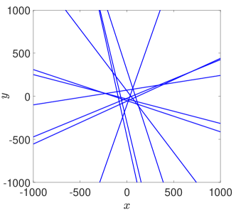
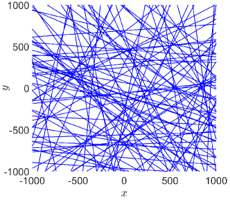
To address these aspects of urban street networks, recently in a short note, we have introduced the binomial line process (BLP) as a new stochastic line process that consists of a deterministic number of lines generated in a bounded generating set [17]. Let us visualize the difference in the network formed by a BLP as compared to a PLP, with the help of realizations of these two candidate line processes (please refer to Section II-A for details on the construction of a BLP). In Fig. 2a, we plot a realization of a BLP where streets are generated within a distance of from the origin. We compare it with a realization of a PLP in Fig. 2b where the generating PPP has an intensity . It is apparent that the BLP captures the varying street and street length densities of a single city by virtue of its non-stationarity while the PLP-based models are stationary and thus restricted to a single fixed density. Consequently, the BLP model is necessary to contrast the performance of downtown users and sub-urban users.
I-C Contributions and Organization
The main contributions of this paper are summarized as follows:
-
•
We characterize the recently introduced BLP and binomial line Cox process (BLCP) models and give a thorough analysis of several radial density characteristics, including the line length radial density and intersection density of the BLP and PLP. We also derive the distance distribution to the nearest intersection from a test point on the BLP.
-
•
We derive the probability generating functional (PGFL) of BLCP and provide a simpler derivation (as compared to [17]) of the distribution to the nearest BLCP point from a test point in the Euclidean plane.
-
•
Leveraging the PGFL, we characterize the transmission success probability in a wireless network where the APs form a BLCP. Such a model can emulate a variety of network scenarios, e.g., Wi-Fi APs in an industrial automation setup, on-street deployment of 5G small cells, etc. In contrast, the commonly used stationary models such as the PLCP are restricted to the homogeneous setting where the transceiver density is fixed everywhere.
-
•
To obtain fine-grained insight into a wireless network modeled by a BLCP, we characterize the meta distribution [18], [19] of the signal-to-interference-plus-noise ratio (SINR). In particular, we first derive the moments of the conditional success probability and employ them to study the mean local delay and the density of successful transmission in the wireless network, which provides insight on the latency and coverage of the network. Second, the Gil-Pelaez inversion theorem results in the exact characterization of the meta distribution.
The rest of the paper is organized as follows. The mathematical preliminaries regarding the construction and statistical characterization of the BLP are presented in Section II, along with the derivation of radial and intersection density, and nearest intersection distance distribution. In Section III we define and characterize the BLCP, its void probability, and the PGFL of the BLCP. Section IV presents an application of the derived framework in studying the transmission success probability in a wireless network. The meta distribution is derived in Section V. In Section VI we present numerical results to discuss the salient features of a wireless network based on a BLCP location model of the APs. Finally, the paper concludes in Section VII.
| Notation | Description |
|---|---|
| Binomial line process | |
| th line of a BLP | |
| Radius of circle in which BLP is generated | |
| A disk of radius centered at | |
| Number of lines of the BLP | |
| Domain band corresponding to | |
| Area of the domain bands corresponding to | |
| Void probability of the BLP with lines on | |
| Void probability of the BLCP with lines on | |
| Density of length of chords/line segments in a bounded Borel set | |
| Density of length of chords/line segments in the th annulus of equal width | |
| Line length measure | |
| Line length density | |
| Average number of intersections within a disk centered at the origin | |
| Density of intersections in the th annulus of equal width | |
| Intersection measure of BLP | |
| Intersection density of BLP | |
| Intersection density of PLP | |
| Area of the domain bands corr. to the nearest intersection from the test point | |
| 1D PPP on | |
| Density of | |
| Length of a chord generated by a line corresponding to on . | |
| Binomial line Cox process with parameters and | |
| SINR received at the test point | |
| Success probability at threshold | |
| Meta distribution evaluated at SINR threshold and reliability threshold |
I-D Notations
Line processes are denoted by calligraphic letters, e.g., , while point processes are denoted by . An instance of a point process is denoted by . A BLP is presumed to consist of lines unless stated otherwise. Capital math-font characters are random variables unless otherwise stated, e.g., , while an instance of is denoted by . Similarly, other scalar quantities are denoted by small letters, e.g., . In the two-dimensional Euclidean plane, , locations are denoted by bold font, e.g., . and represent the expectation and the probability operators, respectively. The other notations used in the paper are summarized in Table I.
II Preliminaries
We will restrict our discussion to due to its relevance to the locations of users and APs in wireless networks.
II-A Binomial Line Process - Construction
A BLP is a finite collection of lines in the two-dimensional Euclidean plane. Formally,
| (1) |
Each line of corresponds to a point of a binomial point process (BPP) defined on the finite cylinder [) . We will call the generating set or the domain set of , and a point , corresponding to a line , the generating point of . The line segment drawn from the origin to forms the normal to the line . The pair of coordinates of any point in has a bijective mapping to a line in .
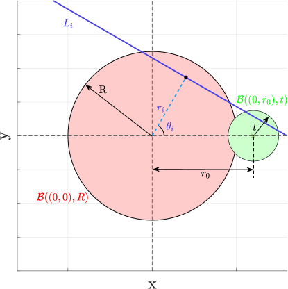
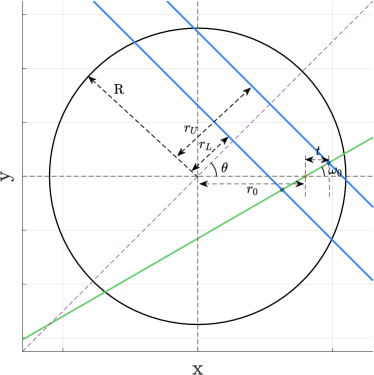
This is illustrated in Fig. 3, where the generating points of the lines are restricted to the disk (shown in red in the figure). It should be noted that the generating points do not form a BPP in but rather in 111The former would imply uniform location of points in the disk, while the latter correspond to uniform distances of the generating points between 0 and .. Furthermore, the BLP is a non-stationary process, and unlike stationary point processes, the statistics of the BLP cannot be characterized from the perspective of a single typical point located, say, at the origin. However, due to the isotropic construction of the BLP, the properties of the BLP as seen from a point depend only on its distance from the origin and not its orientation. Accordingly, without loss of generality, let us consider a test point located at . First, we study the set of lines that intersect a disk of radius centered at the test point , denoted by and shown in green in Fig. 3. This will then lead to the distance distribution of the nearest line as discussed in the next subsection.
II-B Domain Bands in and the Distance Distribution to the Nearest BLP Line
Let us consider the line , where and, the boundary of the disk is . Solving these two equations simultaneously for and , we obtain the abscissa of the intersection points of and as:
| (2) |
In order to find the subset for which the generated lines intersect , we find the which results in being a tangent to . For a given , the value(s) of for which (2) has only one solution is obtained by solving , which results in
| (3) |
Let the two solutions above be represented by and for the positive and the negative signs, respectively. In other words, all the points that fall within the set bounded by the two curves of (3) generate lines in that intersect . Let us denote this set by .
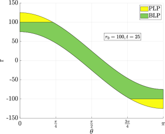
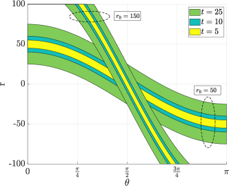
In Fig. 4a, we plot , and due to their structure, is referred to as domain bands. It is interesting to note that the domain band for the BLP is a clipped version of the PLP due to the restriction of the points to lie within . In Fig. 4b, we plot the domain bands for the BLP for different values of and . Naturally, when , the domain bands for BLP and PLP coincide. Additionally, the width of the band decreases as decreases or increases.
Remark 1.
The area of the domain band for a PLP is and is independent of .
The following classical result of the PLP follows.
Corollary 1.
[20] The number of lines of a PLP intersecting is Poisson distributed with parameter . Accordingly, the probability that no lines intersect is given by .
However, in the case of a BLP, the area of the domain band needs to be computed by deriving the angles at which the domain bands are clipped due to its construction (contrary to the PLP where the domain bands are not clipped for any ) [17].
Theorem 1.
[17] The area of the domain band for a BLP is
| (4) |
Corollary 2.
[17] [Void Probability] The probability that no line of the BLP intersects with is
where, is the number of lines of the BLP and is area of the domain bands.
Corollary 3.
[17] The CDF of the distance to the nearest line of the BLP from a test point at is,
II-C Line Length Density and Measure
Recall that one of the objectives of studying the BLP is to emulate different densities of streets in the city center and the suburbs. We characterize it using the line length density and line length measure, defined as follows
Definition 1.
The line length measure is
where is the Lebesgue measure in one dimension and is a line of the BLP. The corresponding radial density is
The line length measure follows by integrating , i.e.,
In order to study the line length density, we first determine the expected total length of chords in a disk, i.e., the line length measure.
Theorem 2.
For a BLP generated by lines within a disk of radius ,
Proof.
Let . We have
| (5) |
where is the number of lines intersecting disk and is the expected length of the chord formed by a single line in the disk . Step (a) follows from the expectation of the binomial distribution. For , is evaluated as
where is obtained from (4).
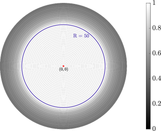
Next, let us consider concentric circles centered at the origin i.e. having radii , where is an integer multiple of . The th annulus is defined as the region between the circles of radii and . Thus, the annuli generated due to these concentric circles have equal width . Using (5) we can find the ratio of the average length of line segments to the area, in the th annulus of width denoted by as
| (6) |
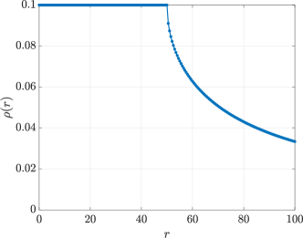
In Fig. 5a we show a grey-scale plot for for and observe that the line length measure in the annuli decreases as increases. Leveraging this, we can characterize the line length density of the BLP as a limiting function of the density in annuli. Precisely, the statement of the theorem is obtained by substituting and taking the limit in (6). ∎
The density remains constant at for and then decreases as as .
II-D Intersection Density
In this section, we study the point process formed by the intersections of the lines of the BLP. Accordingly, we introduce and characterize the intersection measure and the intersection density of the BLP.
Theorem 3.
The radial intersection density at a distance from the origin for a BLP generated by lines within a disk of radius is
Proof.
See Appendix A ∎
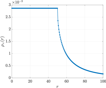
In Fig 6 we see that intersection density first remains constant and then scales as as . By integrating the intersection density, we get the intersection measure
Remark 2.
The intersection measure in the plane is
as expected.
II-E Intersection Density of PLP
In this section, we determine the intersection density and measure of PLP and compare it with that of the BLP.
Theorem 4.
The intersection density for a PLP with density is
Proof.
Let and consider a PLP line generated at the point without loss of generality. The domain band corresponding to the intersection on depends only on the area in which the intersection density is calculated i.e., for a given , the range of where if a line is generated intersects within is,
Consequently, the area of the domain band averaged for uniformly distributed between 0 and can be written as
Accordingly, the probability that a line of the PLP intersects a single line within is
Let us now suppose that lines are generated in . With probability , each of them intersect line . Thus, the average number of intersections on from the lines within is evaluated as
Finally in order to determine the average number of intersections on all the lines within , we take the expectation over the number of lines that are generated within . This is evaluated as
| (7) |
Next, similar to subsection 2.3, we consider concentric circles centered at the origin having radii . As a result, the annuli formed by these concentric circles have the same width, . In the th annulus of width , we use (7) to determine the ratio of the average number of intersections to the area to find the intersection density
| (8) |
This implies that the density at any point at any distance from the origin is also constant. ∎
As expected, the intersection density scales as .
II-F Distance Distribution to the Nearest Intersection
Let us consider a test point that lies on a line of the BLP. Consequently, lines of the BLP intersect the line containing the test point almost surely. Let be the distance to the nearest intersection from the test point. Also, let be the angle formed between the line passing through and the x-axis. This is illustrated in Fig. 7, where for an intersection to be located at a distance of from the test point at an angle of , there may exist a set of for a given wherein no lines should be generated. Accordingly, in order to find the distance distribution, we need the set of all such for which lines do not intersect the line passing through at an angle of within a distance of from the test-point. Now, for a given , the range of where if a line is generated, intersects the test point within a distance is calculated as:
| (9) |
| (10) |
The above equations of and are obtained using simple trigonometric calculations and include all possible cases for different values of , and . As an example, the case presented in Fig. 7 corresponds to and , accordingly, we have . We see that when we can end up with scenarios , thus equation (9) and (10) have been defined in such a way that will always be less than for all possible values of and . Also, (9) and (10) consider the cases when and exceed .
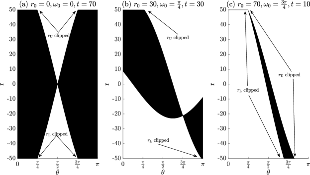
Let be the set of all such for which lines do not intersect the line passing through at angle of within a distance of from the test-point. Fig. 8 shows some examples of the domain band regions wherein a line should not be generated for it to not intersect the line passing through within a distance from the test point at an angle of . In Fig 8(a), as and we see that , the domain bands are getting clipped at 50 and -50 for most of the initial and final values of . Likewise in Fig. 8 (c) when the test point lies outside the circle of radius and i.e., and, more values of and are clipped for and the total width of the band is also small, thus showcasing that test points lying outside and having small would experience fewer intersections.
Corollary 4.
For a BLP line passing through , the CDF of the distance to the nearest intersection is
The area of for a BLP defined on corresponding to and is Accordingly, the probability that no line of the BLP intersects the line passing through within a distance from the test point is given by

In Fig. 9 we plot the CDF for different values of and for . We see that the nearest intersection is closer for higher and smaller values.
III Binomial Line Cox Process
On each line of , let us define an independent 1D PPP with intensity . A BLCP , is the collection of all such points on all lines of the BLP, i.e., . Thus, the BLCP is a doubly-stochastic or Cox process of random points defined on random lines.
III-A Void Probability
Similar to the BLP, we derive the void probability of the BLCP and consequently, its nearest point distance distribution. This has previously been reported in [17], however, compared to [17], we take a simpler approach for the derivation. In particular, leveraging the polar coordinates leads to much simpler trigonometric manipulations, and accordingly, we reduce the number of events for which void probability needs to be calculated explicitly.
Theorem 5.
The probability that the disk contains no points of is given by
| (11) |
where,
| (12) |
is the length of the chord created by a line corresponding to in the disk .
Proof.
Let us first consider a line generated by a uniformly located point in and the corresponding BLCP (which is simply a 1D PPP) defined on this line. Then the void probability for a single line case can be found as,
| (13) |
The void probability is the probability that no BLP lines contain a BLCP point inside . Let us recall that the distance of a line corresponding to from the test point is, . Accordingly, if , then does not intersect resulting in a chord length 0. Then, given that , the probability that no points of the BLCP lie on that chord is given as following the void probability of a PPP with intensity . Due to the independence of the locations of the generating points in and the independence of the individual 1D PPPs , the void probability can be evaluated as
| (14) |
∎
Corollary 5.
[Distance Distribution] Following the void probability, the distance distribution of the nearest BLCP point from the test point is
III-B Palm Perspective of the BLCP
Next, we study the BLCP from the perspective of a point of the process itself, using Palm calculus222In point process theory, the Palm probability refers to the probability measure conditioned on a point of the process being at a certain location [21].. Let us recall that for a PLCP with as the density of the points on the lines, we have , where is a 1D PPP on a line that passes through the origin. In other words, the Palm distribution, i.e., conditioning on a point of the PLCP to be at the origin, is equivalent to adding (i) an independent Poisson process of intensity on a line through the origin with uniform independent angle and (ii) an atom at the origin to the PLCP. Similarly, for a BLCP, conditioning on a point to be located at is equivalent to considering an atom at , a 1D PPP on a line passing through and a BLCP defined on a BLP consisting of lines in the same domain. Thus, the Palm measure of the BLCP can be expressed as follows.
Lemma 1.
For a BLCP defined on a BLP with lines, we have
| (15) |
where is a 1D PPP on a randomly oriented line that passes through .
The Palm perspective is necessary to characterize the statistics of the performance metrics conditioned on an event that a node, e.g., a transmitter or an AP is located at a given point. For example, consider a network in which the location of the APs are modeled according to a BLCP. If a receiver located at the origin associates with a transmitter located at , then the interfering APs are located not only in the other lines but also on a line necessarily passing through . The applications of this concept will be evident in the next section where we employ the derived framework to analyze a wireless communication network. Prior to that, let us derive the PGFL of the shifted and reduced point process by conditioning on the location of the nearest point from the origin.
III-C Probability Generating Functional
Here, we characterize the PGFL of the BLCP . The PGFL of a point process evaluated for a function is defined mathematically as the Laplace functional of and is calculated as . In this paper, we are interested in isotropic functions that depend only on the distance of the points from the origin, i.e., we consider functions of the form .
Definition 2.
Let be the nearest point of a BLCP from . Then, the shifted and reduced point process is defined as .
The motivation for studying the properties of in the context of wireless networks is as follows; if the AP locations are modeled as a BLCP, then represents the locations of the interfering APs from the perspective of a user located at a distance from the origin and connected to an AP located at a distance from the user. The next theorem characterizes the PGFL for the shifted and reduced BLCP .
Theorem 6.
For a shifted and reduced BLCP defined on a BLP with lines generated within , the PGFL of a function conditioned on is given as
where is the distance to the nearest point of from the origin. Consequently, the PGFL of is evaluated as , where the distribution of is given by Corollary 5.
Proof.
Let be a positive, measurable, monotonic, and bounded function for the first part of the proof. Here we will find the PGFL of the point process . In other words, the shifted and reduced point process of interest is restricted to the disk centered at the origin with radius . The theorem follows from the monotone convergence theorem with . Recall that for a PPP of intensity and a function , the PGFL is [22]:
| (16) |
Next, note that the distance of a BLP line corresponding to the generating point in from the origin in is . A point located at a distance from the perpendicular projection of to , has a distance from . The length of the chord is when .
where step (a) is due to the monotone convergence theorem. In , each line can be either of two types (a) intersecting with and (b) non-intersecting with , where is the distance from the origin to the nearest point of . For a particular and , a line is intersecting if and non-intersecting otherwise. Thus, we can write the conditional PGFL of the intersecting and non-intersecting lines after averaging over as
| (17) |
Next, note that the line containing the nearest point (at a distance ) of the BLCP intersects the disk almost surely. Whereas, the other lines may or may not intersect the disk depending on their generating point. Accordingly, the PGFL for is evaluated as
| (18) |
In step (a), the term corresponds to the line containing the nearest point (recall the Palm perspective discussed in the previous sub-section). The term corresponds to the probability that a set of lines intersect the disk and the conditional PGFL given that the lines intersect the disk. The term corresponds to the probability that a set of lines do not intersect the disk and the conditional PGFL given that the lines do not intersect the disk. The statement of the theorem follows from the above. ∎
IV Application - Transmission Success Probability in Wireless Networks
In wireless networks, several performance metrics are studied using the transmission success probability. It is the complementary cumulative density function (CCDF) of the SINR over the fading coefficients and the spatial process governing the locations of the APs. In this section, first we define this metric and then we characterize it using the results derived in the previous sections.
IV-A Success Probability - Definition
Let be a point process (not necessarily a BLCP) consisting of points , . Consider a separate test point located at the origin. For convenience, let us assume that the points of are ordered according to their distance from the origin, i.e., . If the points of emulate the locations of the APs of a wireless network relative to a receiver located at the origin, the receiver connects to the AP located at . This is known as the nearest-AP association.
Each wireless link experiences fluctuations of the received power due to constructive and destructive superposition of multiple reflecting paths in the propagation environment. This is termed small-scale fading. Classically, the impact of this is taken into account by multiplying the received signal with a random variable with exponential distribution with parameter 1 [23]. For a path-loss exponent , the SINR is
| (19) |
where is a constant that takes into account the transmit power, AWGN noise, path-loss constant, as well as the transmit and receive antenna gains. We assume that this parameter is the same for each transmit node. Typically, each is independent of each other and identically distributed [23]. For the ease of notation, let us represent by . Now, the transmission success probability at a threshold of is defined as the CCDF of [23]:
| (20) |
This represents the probability that an attempted transmission by the nearest AP located at is decoded successfully by the receiver at the origin. In what follows, we refer to the transmission success probability as success probability.
IV-B Success probability for BLCP Locations of APs
The BLCP is a relevant model for studying deployment locations of APs along the streets of a city, or e.g., along alleyways of industrial warehouses. As discussed before, the analysis of the network performance depends on the location of the test point222It may be noted that the wireless network performance analyzed at the test point referred here corresponds to the performance evaluated at the typical point at a location of a stationary receiver point process.. However, since the BLP is isotropic, we may infer that its properties as seen from a point only depend on its distance from the center and not its orientation. Accordingly, the test point can be considered to be located along the x-axis, i.e., we analyze the performance from the perspective of a test point located at , without loss of generality. Equivalently, we can consider the receiver at the origin and study the statistics of the shifted point process . Let us assume that the receiver establishes a connection with its nearest AP (i.e., the AP located at the nearest BLCP point from the receiver), consequently experiencing interference from all other APs. In such a case, the success probability is characterized by the following result.
Theorem 7.
Proof.
The success probability can be evaluated as
| (21) |
Here, refers to the expectation taken with respect to the Palm probability of the shifted and reduced point process, i.e., conditioned on a point of being located at and then removing it. The 1st term, , takes into account the impact of the noise and thus only depends on and . The second term , takes into account the impact of the interference and can be further simplified
Employing the above in (21) completes the proof. ∎
Corollary 6.
For and , the PGFL of for the function is given as
One important metric of interest, especially for broadband applications, is the complementary CDF of the data rate. Let us recall that according to Shannon’s formula, the instantaneous channel capacity is . Now, for a packet deadline of and a file size for low-latency communications, the communication rate (in terms of bits per second) should be sustained at or higher.
Corollary 7.
The probability that the instantaneous channel capacity is or higher can be evaluated using the success probability as
V Application - Meta Distribution of the SINR in BLCP
Although the success probability is a useful metric for planning a wireless network and tuning network parameters, it only provides an average view of the network across all possible realizations of . This inhibits the derivation of a fine-grained view into the network. In this regard, the meta distribution, i.e., the distribution of the success probability conditioned on provides a framework to study the same [18, 19]. The conditional success probability, i.e., is a random variable due to the random . It is precisely this random variable whose statistics we want to study. Its CCDF, called the meta distribution of the SINR, is given as
| (22) |
which is a function of two parameters and . In addition, consider another important aspect of wireless networks — not all transmitters transmit simultaneously but are controlled by an access scheme. In particular, let us assume a simple ALOHA access scheme wherein, when the connected AP transmits, each interfering AP transmits with a probability [24]. Thus, each interference term is weighted by the probability of the corresponding node transmitting. Let the set of locations of the interfering nodes be denoted by . In this scheme, the conditional success probability can be obtained similarly to the success probability as
Step (a) is due to the exponential distribution of . Step (b) follows from the Laplace transform of the exponentially distributed . In general, directly deriving the distribution of the random variable is most likely impossible. The standard approach to circumvent this challenge is by first deriving its moments and then transform them to the distribution [25].
Theorem 8.
The th moment of conditioned on for any is given as
where . Taking an expectation over (see Corollary 5) results in the unconditioned th moment.
Proof.
We have
| (23) |
∎
Step (c) follows because the expectation is over , thus the first term comes out of expectation. Step (d) follows from the PGFL of the BLCP. Consequently, the meta distribution of the SINR can be calculated using the Gil-Palaez theorem as [26]
where is the imaginary part of the argument and .
Corollary 8.
For , the first moment of conditioned on can be simplified as
where .
The capacity of a wireless network can be studied in terms of the successful transmission density . This represents the density of the simultaneous transmitters that attempt and experience successful transmissions.
Furthermore, the mean local delay is the expected number of transmissions required for successful transmission. It is obtained by setting [26]. Naturally, in the case of latency-constrained networks, this is a critical parameter.
Corollary 9.
For , the mean local delay conditioned on is
where
where .
In the next section, we discuss how due to the impact of interference, optimizing the channel access probability for minimizing the mean local delay is non-trivial.
VI Numerical Results and Discussion
In this section, we discuss some numerical results to highlight the applications of the derived framework in analyzing the wireless network. Unless otherwise stated, all results are for and, .
VI-A On the Success Probability
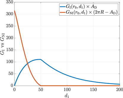
First, let us observe some features of the weighted conditional PGFLs and
for the function as derived in (17)). From (18) note that these conditional PGFLs constitute the overall functional , i.e.,
Moreover, since is proportional to for a given , it is important to study the trends in the weighted conditional PGFLs with . For lower values of , is smaller than . Accordingly, Fig. 10 shows that has a value at and decreases with until it becomes zero exactly at . This is due to the fact that at , all lines intersect the disk. On the contrary, has a value 0 at and increases till , as the area corresponding to intersecting lines increases. Beyond , decreases precisely due to the increasing distance of the serving AP from the receiver.
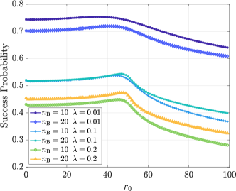
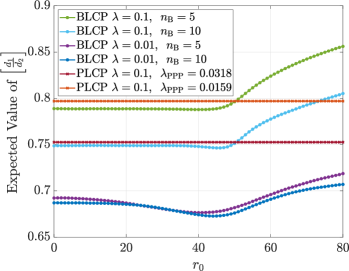
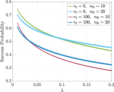
In Fig. 11a, we plot the success probability with respect to for different values of and . We observe that the success probability first increases slightly with , reaches a maximum and starts decreasing. To delve deeper into this phenomenon, we plot the expected value of the ratio of the distance from the nearest BLCP point to the distance of the second nearest BLCP point with respect to . In systems where the majority of the interference power is contributed by the nearest interferer, this parameter acts as a good indicator of the success probability. From Fig. 11b, we note that the value of decreases with at first, reaches its minimum value near and increases beyond that. This indicates that as we move away from the city center, although both the serving AP and the interferers become statistically distant from the test point, the relative increase in is higher as compared to the relative increase in with . Such an insight for urban networks, in case the streets follow a BLCP cannot be obtained with PLCP models (also shown in Fig. 11b for different densities).
VI-B Optimal Network Parameters
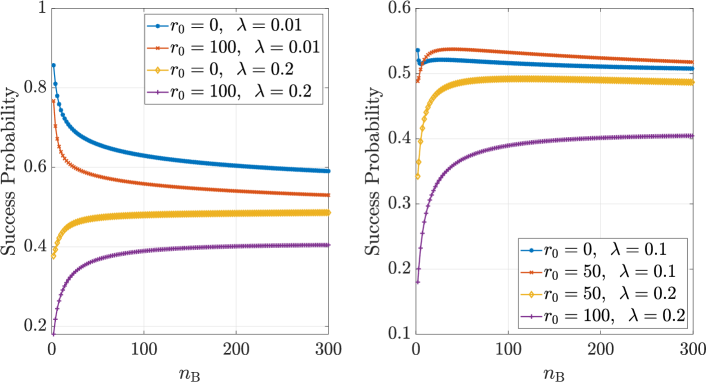
In Fig. 12 and Fig. 13 we plot the success probability with respect to and respectively for different values of . We observe that for a given location of the test device, increasing the number of lines may increase or decrease the success probability depending on the location of the test device and the density of deployment. In particular, the results suggest that a higher number of APs are needed to be deployed in a scenario with dense streets. Based on the location of the test device, there may exist an optimal deployment density of the APs. For example, for a test device located at , a deployment density of maximizes the coverage. Fig. 13 shows that as increases the coverage decreases, due to the increased interference. After a certain value, more streets provide better coverage than fewer streets. Similarly, in Fig. 12(b), we observe that maximizes coverage for a given and . Also, for high values of , coverage increases with and then decreases.
VI-C Results on Moments of Conditional Success Probability and Meta Distribution
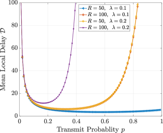
In Fig. 14a we plot the mean local delay for a test node present at the origin. As the transmit probability increases, we see that initially, the local delay decreases since the transmitter accesses the channel more frequently. However, as the transmit probability increases, a higher density of interfering APs results in the deterioration of the coverage and accordingly, an increase in the delay. This indicates the existence of optimal transmit probability for minimizing the delay. The optimal transmit probability for minimizing the mean local delay is non-trivial to derive due to the two contending phenomena - increasing i) increases the frequency with which the service to the test device is attempted thereby reducing the delay and ii) increases the interference which reduces the transmission success and increases the delay. Such nuances of the wireless network are kept for future study.
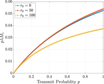
Fig. 14b shows the successful transmission density, , which is the number of successful transmissions per unit area. This acts as an indicator of the network capacity. Here we have assumed , , and dB. We see that increases as increases specifying that more transmission leads to better transmission density. As we move closer to the city edge i.e., successful transmission density increases slightly as compared to due to reduced interference. However, at a further distance from the city center, the successful transmission density decreases due to the increasing distance from the serving AP. This is consistent with the results of Fig. 11a where we see that as increases coverage first increases then decreases. Such characteristics of the network as a function of cannot be obtained using classical models such as PLP and PLCP.
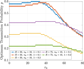
The optimal transmit probability for minimizing the mean local delay is plotted in Fig. 15a for different locations of the test node, , , and . We observe that as increases, also increases first and then decreases. We see that the maximum value of occurs near the edge of the domain of the BLP. As increases further, the distance to the nearest transmitter as well as the other interfering nodes increases. Consequently, the transmit probability reduces in order to limit the device outage. Interestingly, for , for is higher as compared to since the lines are densely packed around the city center. On the contrary, for , needs a higher transmission probability than the case with .
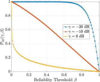
The meta distribution of the success probability is plotted in Fig. 15b with respect to the reliability threshold , for and . We observe that for an SINR threshold of dB, the majority of the users are under coverage with reliability of (or probability 0.7). On the contrary, for a service characterized by dB, with a 90% guarantee, it can be claimed that none of the users will be under coverage. For dB we see that there is a near-linear relationship between the reliability and the number of users under coverage.
VII Conclusions and Future Work
In this paper we have characterized the binomial line Cox process (BLCP) which takes into account the non-homogeneity of lines in a Euclidean plane. Although there are several line processes studied in literature, none of the existing models take into account the non-homogeneity of the lines. This is a drawback of the existing models since practical problems e.g., wireless network planning or transport infrastructure planning need to deal with non-homogeneous streets in a city. We have derived the distribution to the distance of the nearest intersection, the probability generating functional of the BLCP and used it to analyze the transmission success probability in a wireless network. Then, we provide extensive numerical results to derive system design insights for such network deployments. Furthermore, we characterize the meta-distribution of the SINR in order to gain a fine-grained view of the network. We envisage that the statistical model developed in this paper will be employed in the study of practical problems involving urban street planning. The shortest path-length, multi-tier nodes, and non-homogeneous Poisson line Cox processes are indeed interesting directions of research, which will be taken up as a future work.
References
- [1] M. T. Shah, “Codes for BLP and BLCP: Statistical characterization and applications in wireless network analysis.” Github, https://github.com/mt19146/blcp, 2023.
- [2] B. Ripley, “The foundations of stochastic geometry,” The Annals of Probability, vol. 4, no. 6, pp. 995–998, 1976.
- [3] F. Baccelli et al., “Stochastic geometry and architecture of communication networks,” Telecommunication Systems, vol. 7, no. 1, pp. 209–227, 1997.
- [4] H. S. Dhillon and V. V. Chetlur, “Poisson line Cox process: Foundations and applications to vehicular networks,” Synthesis Lectures on Learning, Networks, and Algorithms, vol. 1, no. 1, pp. 1–149, 2020.
- [5] G. Mansfield, “Using Streetlights to Boost 5G Deployments in Cities,” https://about.att.com/innovationblog/2022/streetlights-to-boost-5g-deployments.html, February 25, 2022.
- [6] “NYC allows 5G equipment on streetlamps,” https://www.fiercewireless.com/5g/nyc-allows-5g-equipment-streetlamps, 2020.
- [7] W. S. Kendall, “From random lines to metric spaces,” The Annals of Probability, vol. 45, no. 1, pp. 469–517, 2017.
- [8] J. Kahn, “Improper Poisson line process as SIRSN in any dimension,” The Annals of Probability, vol. 44, no. 4, pp. 2694–2725, 2016.
- [9] J. P. Jeyaraj and M. Haenggi, “Cox models for vehicular networks: SIR performance and equivalence,” IEEE Transactions on Wireless Communications, vol. 20, no. 1, pp. 171–185, 2020.
- [10] N. Chenavier and R. Hemsley, “Extremes for the inradius in the Poisson line tessellation,” Advances in Applied Probability, vol. 48, no. 2, pp. 544–573, 2016.
- [11] V. V. Chetlur, Stochastic Geometry for Vehicular Networks. PhD thesis, Virginia Tech, 2020.
- [12] G. Ghatak, A. De Domenico, and M. Coupechoux, “Small cell deployment along roads: Coverage analysis and slice-aware rat selection,” IEEE Transactions on Communications, vol. 67, no. 8, pp. 5875–5891, 2019.
- [13] V. V. Chetlur and H. S. Dhillon, “Coverage and rate analysis of downlink cellular vehicle-to-everything (C-V2X) communication,” IEEE Transactions on Wireless Communications, vol. 19, no. 3, pp. 1738–1753, 2019.
- [14] V. V. Chetlur and H. S. Dhillon, “On the load distribution of vehicular users modeled by a Poisson line Cox process,” IEEE Wireless Communications Letters, vol. 9, no. 12, pp. 2121–2125, 2020.
- [15] C. Gloaguen, “Modelisation macroscopique geometrique des reseaux d’acces en telecommunication,” Presentation at Société de Mathématiques Appliquées et Industrielles. Link: http://smai.emath.fr/spip/IMG/ppt, 2010.
- [16] T. Courtat, C. Gloaguen, and S. Douady, “Mathematics and morphogenesis of cities: A geometrical approach,” Phys. Rev. E, vol. 83, p. 036106, Mar 2011.
- [17] G. Ghatak, “Binomial line processes: Distance distributions,” IEEE Transactions on Vehicular Technology, vol. 71, no. 2, pp. 2176–2180, 2022.
- [18] M. Haenggi, “Meta distributions—Part 1: Definition and examples,” IEEE Communications Letters, vol. 25, no. 7, pp. 2089–2093, 2021.
- [19] M. Haenggi, “Meta distributions—Part 2: Properties and interpretations,” IEEE Communications Letters, vol. 25, no. 7, pp. 2094–2098, 2021.
- [20] F. Morlot, “A population model based on a Poisson line tessellation,” in 2012 10th International Symposium on Modeling and Optimization in Mobile, Ad Hoc and Wireless Networks (WiOpt), pp. 337–342, 2012.
- [21] M. Haenggi, Stochastic geometry for wireless networks. Cambridge University Press, 2012.
- [22] D. Stoyan, W. S. Kendall, S. N. Chiu, and J. Mecke, Stochastic geometry and its applications. John Wiley & Sons, 2013.
- [23] M. Haenggi et al., “Stochastic geometry and random graphs for the analysis and design of wireless networks,” IEEE Journal on Selected Areas in Communications, vol. 27, no. 7, pp. 1029–1046, 2009.
- [24] N. Abramson, “The aloha system: Another alternative for computer communications,” in Proceedings of the November 17-19, 1970, Fall Joint Computer Conference, AFIPS ’70 (Fall), p. 281–285, Association for Computing Machinery, 1970.
- [25] X. Wang and M. Haenggi, “Hausdorff moment transforms and their performance,” arXiv preprint arXiv:2212.12622, 2022.
- [26] M. Haenggi, “The meta distribution of the SIR in Poisson bipolar and cellular networks,” IEEE Transactions on Wireless Communications, vol. 15, no. 4, pp. 2577–2589, 2016.
Appendix A Proof of Theorem 3
Let and assume that the BLP is generated within a circle of radius of with lines. In order to determine the average number of intersections over , let us consider a BLP line generated at the point where . First, let us determine the domain band corresponding to the intersection on i.e., all such for which lines will intersect line within . For a given , the range of where if a line is generated intersects within is,
We see that for values of domain band gets clipped to and in the upper and lower limits, thus the area of the domain band for these two cases i.e. and can be derived as follows.
Case 1: . Here . Consequently, there is no clipping in the values of and the area of the domain band averaged for uniformly distributed between 0 and can be written as
Case 2: . Here . Accordingly, the values of are limited to and . The values of for which are clipped are
We see that is clipped to for values of from to , similarly would be clipped to for values of from to . Thus the area of the domain band averaged for uniformly distributed between 0 and is
Thus, the area of the domain band for a line to intersect the line within is
| (24) |
Accordingly, the probability that a line of the BLP intersects a single line within is obtained by . It is given as
Now, let us assume that lines are generated in . Each of these intersects with probability . As a result, the average number of intersections on within from the lines is evaluated as
Finally in order to determine the average number of intersections on all the lines within , we take the expectation over the number of lines are generated within . This is evaluated as
where corresponds to choosing out of lines, refers to the probability that exactly lines are generated in , is the average number of intersections on a single line given that lines are generated in , is due to the fact that including there are lines in , and finally, is to avoid the double counting of the intersections. Similarly, in case there are lines generated, thus the average number of intersections on all lines is
Combining the above, the average number of intersections within a disk of radius centered at the origin is
| (25) |
Next, similar to subsection 2.3, we consider concentric circles centered at the origin having radii . As a result, the annuli formed by these concentric circles have the same width, . In the th annulus of width , we use (25) to determine the ratio of the average number of intersections to the area to determine intersection radial density as,
| (26) |
The final result of the intersection radial density of a BLP can be obtained by substituting and taking the limit in (26).