Online Planning of Uncertain MDPs under Temporal Tasks
and Safe-Return Constraints

Abstract

This paper addresses the online motion planning problem of mobile robots under complex high-level tasks. The robot motion is modeled as an uncertain Markov Decision Process (MDP) due to limited initial knowledge, while the task is specified as Linear Temporal Logic (LTL) formulas. The proposed framework enables the robot to explore and update the system model in a Bayesian way, while simultaneously optimizing the asymptotic costs of satisfying the complex temporal task. Theoretical guarantees are provided for the synthesized outgoing policy and safety policy. More importantly, instead of greedy exploration under the classic ergodicity assumption, a safe-return requirement is enforced such that the robot can always return to home states with a high probability. The overall methods are validated by numerical simulations.

I Introduction

Uncertainty arises in various aspects of robot motion planning such as the model of the workspace and the outcome of motion execution. Markov Decision Process (MDP) is a convenient way to model such uncertain systems [1] based on which decision making problems are solved to optimize a given control objective. The most common objective is to reach a set of goal states while minimizing the expected total cost. The resulting solution is a policy that maps states to probability distributions over the set of allowed actions [1]. Furthermore, there have been many efforts to address the problem of synthesizing a control policy for a MDP that satisfies high-level temporal tasks. Most common control objectives such as reachability, surveillance, liveness and emergency response, can be specified via temporal logic formulas. There has been numerous work considering different formal languages, such as Probabilistic Computation Tree Logic (PCTL) and Linear Temporal Logics (LTL), see[2]. Such tasks are normally specified over regions of interest in the state space. A verification toolbox is provided in [3] for MDPs under certain LTL tasks. Different cost optimizations are also considered such as maximum reachability in [4], the minimal bottleneck cost in [2], the pareto resource constraints in [5], the balanced satisfiability and cost in [6], and the uncertainty over semantic maps in [7].

However, under limited information, even the underlying MDP could be uncertain, e.g., the transition measure or the state features is only partially-known, the above techniques can not be applied directly. Thus, robust control policies are synthesized offline in [8] to maximize the accumulated time-varying rewards, in [9] to maximize the satisfiability under uncertain transition measures, and in [10] to improve multi-robot team performance for dynamic workspaces. These policies are mostly constructed offline. In contrast, online approaches require the robot to actively explore and learn the system model and the optimal policy simultaneously during run time. The work in [11] introduces exploration bonus to balance exploration and exploitation during learning. To guarantee convergence, most existing exploration algorithms rely on the assumption of ergodicity that any state in the MDP is reachable from any other state under a suitable policy [12]. Thus, any state can be safely explored and consequently the system model around that state. Nonetheless, this assumption does not hold in many practical examples where the system would break once entering an unsafe state, e.g., a ground vehicle falls off stairs, or enters a room via a one-way door. Thus, safe exploration during learning has been an active research topic, see [13]. Nonetheless, complex temporal tasks have not been well studied within non-ergodic systems that are partially-unknown.

To overcome these issues, this work proposes an online planning and exploration method for robotic systems modeled as uncertain MDPs. It allows the robot to gradually improve the model and thus the asymptotic cost of the complex task, while ensuring that it can always safely return to a set of home states. The main contribution lies in the novel framework for general uncertain MDPs, which can handle complex temporal tasks and ensure real-time safety during the learning processes.

II Preliminaries

II-A Linear Temporal Logic (LTL)

The ingredients of a LTL formula are a set of atomic propositions $AP$ and several Boolean and temporal operators. Atomic propositions are Boolean variables that can be either true or false. A LTL formula is specified according to the syntax [4]: $\varphi\triangleq\top\;|\;p\;|\;\varphi_{1}\wedge\varphi_{2}\;|\;\neg\varphi\;|\;\bigcirc\varphi\;|\;\varphi_{1}\,\textsf{U}\,\varphi_{2},$ where $\top\triangleq\texttt{True}$, $p\in AP$, $\bigcirc$ (next), U (until) and $\bot\triangleq\neg\top$. We omit the derivations of other operators like $\square$ (always), $\Diamond$ (eventually), $\Rightarrow$ (implication). Given any word $w$ over $AP$, it can be verified whether $w$ satisfies the formula, denoted by $w\models\varphi$. The full semantics and syntax of LTL are omitted here, see e.g., [4].

II-B Deterministic Rabin Automaton (DRA)

The set of words that satisfy a LTL formula $\varphi$ over $AP$ can be captured through a Deterministic Rabin Automaton (DRA) $\mathcal{A}_{\varphi}$ [4], defined as $\mathcal{A}_{\varphi}\triangleq(Q,\,2^{AP},\,\delta,\,q_{0},\,\text{Acc}_{\mathcal{A}})$, where $Q$ is a set of states; $2^{AP}$ is the alphabet; $\delta\subseteq Q\times 2^{AP}\times{Q}$ is a transition relation; $q_{0}\in Q$ is the initial state; and $\text{Acc}_{\mathcal{A}}\subseteq 2^{Q}\times 2^{Q}$ is a set of accepting pairs, i.e., $\text{Acc}_{\mathcal{A}}=\{(H^{1}_{\mathcal{A}},I^{1}_{\mathcal{A}}),(H^{2}_{\mathcal{A}},I^{2}_{\mathcal{A}}),\cdots,(H^{N}_{\mathcal{A}},I^{N}_{\mathcal{A}})\}$ where $H^{i}_{\mathcal{A}},\,I^{i}_{\mathcal{A}}\subseteq Q$, $\forall i=1,2,\cdots,N$. An infinite run $q_{0}q_{1}q_{2}\cdots$ of $\mathcal{A}$ is accepting if there exists at least one pair $(H^{i}_{\mathcal{A}},\,I^{i}_{\mathcal{A}})\in\text{Acc}_{\mathcal{A}}$ such that $\exists n\geq 0$, it holds $\forall m\geq n,\,q_{m}\notin H^{i}_{\mathcal{A}}$ and $\overset{\infty}{\exists}k\geq 0$, $q_{k}\in I^{i}_{\mathcal{A}}$, where $\overset{\infty}{\exists}$ stands for “existing infinitely many”. Namely, this run should intersect with $H^{i}_{\mathcal{A}}$ finitely many times while with $I^{i}_{\mathcal{A}}$ infinitely many times. There are translation tools [14] to obtain $\mathcal{A}_{\varphi}$ given $\varphi$ with complexity $2^{2^{\mathcal{O}(|\varphi|\log|\varphi|)}}$.

III Problem Formulation

III-A Probabilistically-labeled MDP

We extended the probabilistically-labeled MDP proposed in our earlier work [6] to include uncertainty in robot motion and workspace properties:

$$\mathcal{M}\triangleq(X,\,U,\,D,\,p_{D},\,(x_{0},\,l_{0}),\,AP,\,L,\,p_{L},\,c_{D}),$$ (1)

where $X$ is the finite state space; $U$ is the finite control action space and $U(x)$ denotes the set of actions allowed at state $x\in X$; $D\triangleq\{(x,u)\,|\,x\in X,\,u\in U(x)\}$ is the set of possible state-action pairs; $p_{D}\colon X\times U\times X\rightarrow{[0,1]}$ is the transition probability and $\sum_{\check{x}\in X}p_{D}(x,u,\check{x})=1$, $\forall(x,\,u)\in D$; $c_{D}\colon D\rightarrow\mathbb{R}^{>0}$ is the cost function; $AP$ is a set of atomic propositions as the properties of interest;  $L\colon X\rightarrow 2^{2^{AP}}$ returns the properties held at each state; and $p_{L}\colon X\times 2^{AP}\rightarrow{[0,\,1]}$ is the associated probability. Note that $\sum_{l\in L(x)}p_{L}(x,\,l)=1$, $\forall x\in X$;and $x_{0}\in X$, $l_{0}\in L(x_{0})$ are the initial states and labels.

III-B Uncertainty and Bayesian Learning

However, due to limited initial knowledge, the above MDP is uncertain. Particularly, for each pair $(x,u)\in D$, the distribution over its post states follows the Dirichlet distribution [15] with parameter $\boldsymbol{\alpha}_{x}^{u}$:

$$p_{D}\sim\text{Dirichlet}(\boldsymbol{b}_{x}^{u},\,\boldsymbol{\alpha}_{x}^{u}),$$ (2)

where $\boldsymbol{b}_{x}^{u}\triangleq\{b_{0},b_{1},\cdots,b_{K_{x}^{u}}\}$, where $b_{k}$ is a vector of length $K_{x}^{u}$ with one at index $k$ and the remaining elements are zero, $\forall k=0,\cdots,K_{x}^{u}$; $\boldsymbol{\alpha}_{x}^{u}\triangleq\{\alpha_{x}^{u}(\check{x}),\forall\check{x}\in\mathcal{K}_{x}^{u}\}$ is a set of non-negative scaling coefficients with $\alpha_{x}^{u}(\check{x})\geq 0$; also $\mathcal{K}_{x}^{u}\triangleq|\check{x}\in X\,|\,p_{D}(x,u,\check{x})>0|$, and $K_{x}^{u}\triangleq|\mathcal{K}_{x}^{u}|$.

Similarly, for each $x\in X$, the distribution over its labels also follows the Dirichlet distribution with parameter $\boldsymbol{\alpha}_{x}^{L}$:

$$p_{L}\sim\text{Dirichlet}(\boldsymbol{b}_{x}^{L},\,\boldsymbol{\alpha}_{x}^{L}),$$ (3)

where $\boldsymbol{b}_{x}^{L}\triangleq\{b_{0},b_{1},\cdots,b_{K_{x}^{L}}\}$ is defined similarly to $\boldsymbol{b}_{x}^{u}$; $\boldsymbol{\alpha}_{x}^{L}\triangleq\{\alpha_{x}^{L}(l),\forall l\in L(x)\}$ is a set of non-negative scaling coefficients $\alpha_{x}^{L}(l)\geq 0$; and $K_{x}^{L}\triangleq|l\in L(x)\,|\,p_{L}(x,l)>0|$. Thus, we denote the complete set of parameters that govern the transition and labeling probability of $\mathcal{M}$ by:

$$\boldsymbol{\alpha}\triangleq\{\boldsymbol{\alpha}_{x}^{u},\,\boldsymbol{\alpha}_{x}^{L},\,\forall(x,u)\in D\},$$ (4)

which is called the belief over $\mathcal{M}$. In the sequel, we use $\mathcal{M}^{\boldsymbol{\alpha}}$ to denote the general class of MDP $\mathcal{M}$ under belief $\boldsymbol{\alpha}$, while $\mathcal{M}$ alone stands for one sample from $\mathcal{M}^{\boldsymbol{\alpha}}$.

Furthermore, the robot is equipped with sensors and thus can observe the actual transitions and labels during motion. Then, the distributions $p_{D}$ and $p_{L}$ can be updated in a Bayesian way by following [16].

III-C Task Specification

Moreover, there is a LTL task formula $\varphi$ specified over the same set of atomic propositions $AP$ as the desired behavior of $\mathcal{M}$, following the syntax in Sec. II-A.

At stage $T\geq 0$, the robot’s past path is given by $X_{T}=x_{0}x_{1}\cdots x_{T}\in X^{(T+1)}$, the past sequence of observed labels is given by $L_{T}=l_{0}l_{1}\cdots l_{T}\in(2^{AP})^{(T+1)}$ and the past sequence of control actions is $U_{T}=u_{0}u_{1}\cdots u_{T}\in U^{(T+1)}$. It should hold that $p_{D}(x_{t},u_{t},x_{t+1})>0$ and $p_{L}(x_{t},l_{t})>0$, $\forall t\geq 0$. The complete past is then given by $R_{T}=x_{0}l_{0}u_{0}\cdots x_{T}l_{T}u_{T}$. Denote by $\boldsymbol{X}_{T}$, $\boldsymbol{L}_{T}$ and $\mathbf{R}_{T}$ the set of all possible past sequences of states, labels, and runs up to stage $T$. We set $T=\infty$ for infinite sequences. Then, the mean total cost [1] of an infinite robot run $R_{\infty}$ of $\mathcal{M}$ is defined as $\textbf{Cost}(R_{\infty})\triangleq\lim_{t\rightarrow\infty}\frac{1}{t}\sum_{t=0}^{\infty}\,c_{D}(x_{t},u_{t})$, where $c_{D}(\cdot)$ is the cost of applying $u_{t}$ and $x_{t}$ from (1). A finite-memory policy is defined as $\boldsymbol{\mu}=\mu_{0}\mu_{1}\cdots$. The control policy at stage $t\geq 0$ is given by $\mu_{t}:\mathbf{R}_{t}\times U\rightarrow[0,1]$, $\forall t\geq 0$. Denote by $\overline{\boldsymbol{\mu}}$ the set of all such finite-memory policies.

Given one sample MDP $\mathcal{M}$ and a policy $\boldsymbol{\mu}$, the set of all infinite runs is denoted by $\mathbf{R}_{\mathcal{M}}^{\boldsymbol{\mu}}\subset\mathbf{R}_{\infty}$. Then the probability of $\mathcal{M}$ satisfying $\varphi$ under  $\boldsymbol{\mu}$ is defined by:

$$\textbf{Sat}_{\mathcal{M}}^{\boldsymbol{\mu}}\triangleq Pr_{{\mathcal{M}}}^{\boldsymbol{\mu}}(\varphi)={Pr}_{\mathcal{M}}^{\boldsymbol{\mu}}\big{(}\mathbf{R}_{\mathcal{M}}^{\boldsymbol{\mu}}\,|\,\boldsymbol{L}_{\infty}\models\varphi\big{)},$$ (5)

where the satisfaction relation “$\models$” is introduced in Sec. II-A. Namely, the satisfiability equals to the probability of all infinite runs whose associated labels satisfy the task. More details on the probability measure can be found in [4]. Moreover, the cost of policy $\boldsymbol{\mu}$ over $\mathcal{M}$ is denoted by

$$\textbf{Cost}_{\mathcal{M}}^{\boldsymbol{\mu}}\triangleq\mathbb{E}_{R_{\infty}\in\mathbf{R}_{\mathcal{M}}^{\boldsymbol{\mu}}}\{\textbf{Cost}(R_{\infty})\},$$ (6)

as the expected mean cost of all possible infinite runs.

III-D Safe-return Constraints

Furthermore, to ensure safety while the robot explores the workspace, we introduce the following definition of safety based on [17]. Particularly, consider two finite-memory policies $\boldsymbol{\mu}_{\texttt{o}},\boldsymbol{\mu}_{\texttt{r}}\in\overline{\boldsymbol{\mu}}$, where $\boldsymbol{\mu}_{\texttt{o}}$ is called the outbound policy that drives the robot to satisfy task $\varphi$ and $\boldsymbol{\mu}_{\texttt{r}}$ is the return policy that ensures the safety constraint below.

Definition 1

Given system $\mathcal{M}$, an outbound policy $\boldsymbol{\mu}_{\texttt{o}}$ is called $\chi_{\texttt{r}}$-safe at stage $t\geq 0$ if there exists a return policy $\boldsymbol{\mu}_{\texttt{r}}$ such that the probability of system $\mathcal{M}$ returning to a set of home states $X_{\texttt{r}}\in X$ is lower-bounded, namely,

$$\textbf{Safe}_{\mathcal{M}}^{\boldsymbol{\mu}_{\texttt{o}},\boldsymbol{\mu}_{\texttt{r}}}\triangleq Pr_{{\mathcal{M}},(x_{t},l_{t})}^{\boldsymbol{\mu}_{\texttt{o}},\boldsymbol{\mu}_{\texttt{r}}}(\Diamond X_{\texttt{r}})\geq\chi_{\texttt{r}},$$ (7)

where $\chi_{\texttt{r}}>0$ is the assigned safety bound, $(x_{t},l_{t})$ are the robot state and label at stage $t$. $\blacksquare$

Note that traditionally safety is defined as the avoidance of a set of unsafe states, see [13], which mostly are policy-independent and given before-hand. Despite its intuitiveness, it has serious drawbacks in scenarios where unsafe states can only be determined during run time, thus unknown beforehand. In contrast, the safety measure in (7) is policy-dependent and can cover the traditional notion.

III-E Problem Statement

Problem 1

Given the class of uncertain MDPs $\mathcal{M}^{\boldsymbol{\alpha}}$ from (1)-(3), and the task specification $\varphi$, our goal is to synthesize the outbound and return polices $\boldsymbol{\mu}_{\texttt{o}},\boldsymbol{\mu}_{\texttt{r}}$ at each stage $t\geq 0$ that solve the constrained optimization below:

$$\begin{split}&\min_{\boldsymbol{\mu}_{\texttt{o}},\boldsymbol{\mu}_{\texttt{r}}\in\overline{\boldsymbol{\mu}}}\;\;\mathbb{E}_{\boldsymbol{\alpha}}\{\textbf{Cost}_{\mathcal{M}}^{\boldsymbol{\mu}_{\texttt{o}}}\}\\ &\;\text{s.t.}\quad\mathbb{E}_{\boldsymbol{\alpha}}\{\textbf{Sat}_{\mathcal{M}}^{\boldsymbol{\mu}_{\texttt{o}}}\}\geq\chi_{\texttt{o}}\;\;\text{and}\;\;\mathbb{E}_{\boldsymbol{\alpha}}\{\textbf{Safe}_{\mathcal{M}}^{\boldsymbol{\mu}_{\texttt{o}},\boldsymbol{\mu}_{\texttt{r}}}\}\geq\chi_{\texttt{r}},\end{split}$$ (8)

where $\boldsymbol{\alpha}$ is the belief from (4), and $\chi_{\texttt{o}},\chi_{\texttt{r}}>0$ are given lower bounds for satisfiability and safety in (5) and (7). The expectation over alpha before the $\textbf{Sat}_{\mathcal{M}}^{\boldsymbol{\mu}_{\texttt{o}}}$ and $\textbf{Safe}_{\mathcal{M}}^{\boldsymbol{\mu}_{\texttt{o}},\boldsymbol{\mu}_{\texttt{r}}}$ is due to the uncertainty in the system model $\mathcal{M}^{\boldsymbol{\alpha}}$. $\blacksquare$

Main difficulty of the above problem comes from the uncertainties in $\mathcal{M}$ and the consideration of complex temporal tasks along with policy-dependent safety constraints.

It is worth noting that the safe-return constraint in (7) can not be treated as an additional task of the original task $\varphi$, as they are surely conflicting objectives. Thus, the methods proposed in [5, 6] that synthesize only one policy $\boldsymbol{\mu}$ to satisfy simultaneously both tasks, can not be applied here. In other words, it is essential to synthesize two polices: $\boldsymbol{\mu}_{\texttt{o}}$ for the actual task and $\boldsymbol{\mu}_{\texttt{r}}$ for the safe-return requirement.

Figure 1: Illustration of the proposed framework.

IV Safety and Task Policy Synthesis

In this section, we describe the key steps to synthesize the safety and task policies. As shown in Fig. 1, both policies are used in the online execution described in the sequel.

IV-A Product Automaton and AMECs

To begin with, we construct the DRA $\mathcal{A}_{\varphi}$ associated with the LTL task formula $\varphi$ via the translation tools [14]. Let it be $\mathcal{A}_{\varphi}=(Q,\,2^{AP},\,\delta,\,q_{0},\,\text{Acc}_{\mathcal{A}})$, where the notations are defined in Sec. II-B. Then we construct a product automaton between the model $\mathcal{M}$ and the DRA $\mathcal{A}_{\varphi}$.

Definition 2

The product $\mathcal{P}\triangleq\mathcal{M}\times\mathcal{A}_{\varphi}$ is a 7-tuple:

$$\mathcal{P}=(S,\,U,\,E,\,p_{E},\,c_{E},\,s_{0},\,\text{Acc}_{\mathcal{P}}),$$ (9)

where: the state $S\subseteq X\times 2^{AP}\times Q$ satisfies $\langle x,\,l,\,q\rangle\in S$, $\forall x\in X$, $\forall l\in L(x)$ and $\forall q\in Q$; the action set $U$ is the same as in (1) and $U(s)=U(x)$, $\forall s=\langle x,l,q\rangle\in S$; $E=\{(s,u)\,|\,s\in S,\,u\in U(s)\}$; the transition probability $p_{E}\colon S\times U\times S\rightarrow{[0,\,1]}$ is defined by

$$p_{E}\big{(}\langle x,l,q\rangle,\,u,\,\langle\check{x},\check{l},\check{q}\rangle\big{)}=p_{D}(x,\,u,\,\check{x})\cdot p_{L}(\check{x},\,\check{l})$$ (10)

where (i) $\langle x,l,q\rangle,\,\langle\check{x},\check{l},\check{q}\rangle\in S$; (ii) $(x,u)\in D$; and (iii) $\check{q}=\delta(q,\,l)$; the cost function $c_{E}\colon E\rightarrow\mathbb{R}^{>0}$ is given by $c_{E}\big{(}\langle x,l,q\rangle,\,u\big{)}=c_{D}(x,u)$, $\forall\big{(}\langle x,l,q\rangle,\,u\big{)}\in E$. Namely, the label $l$ should fulfill the transition condition from $q$ to $\check{q}$ in $\mathcal{A}_{\varphi}$; the single initial state is $s_{0}=\langle x_{0},l_{0},q_{0}\rangle\in S$; the accepting pairs are defined as $\text{Acc}_{\mathcal{P}}=\{(H^{i}_{\mathcal{P}},\,I^{i}_{\mathcal{P}}),i=1,\cdots,N\}$, where $H^{i}_{\mathcal{P}}=\{\langle x,l,q\rangle\in S\,|\,q\in H^{i}_{\mathcal{A}}\}$ and $I^{i}_{\mathcal{P}}=\{\langle x,l,q\rangle\in S\,|\,q\in I^{i}_{\mathcal{A}}\}$,  $\forall i=1,\cdots,N$. $\blacksquare$

The product $\mathcal{P}$ computes the intersection between the traces of $\mathcal{M}$ and the words of $\mathcal{A}_{\varphi}$, to find the admissible robot behaviors that satisfy the task $\varphi$. It combines the uncertainty in robot motion and the workspace model by including both $x$ and $l$ in the states. For simpler notation, let $\mathcal{K}_{s}^{u}=\{\check{s}\in S\,|\,p_{E}(s,u,\check{s})>0\}$ and $K_{s}^{u}=|\mathcal{K}_{s}^{u}|$. Note that since $\mathcal{M}$ is uncertain under belief $\boldsymbol{\alpha}$, we denote by $\mathcal{P}^{\boldsymbol{\alpha}}$ the general class of product automata associated with each sample MDP within $\mathcal{M}^{\boldsymbol{\alpha}}$. Lastly, the set of home states in $\mathcal{P}$ is denoted by $S_{\texttt{r}}\triangleq\leavevmode\nobreak\ \{s\in S\,|\,s=\langle x,l,q\rangle,x\in X_{\texttt{r}}\}$.

The accepting condition of $\mathcal{P}$ is the same as in Sec. II-B. To transform this condition into equivalent graph properties, we first compute the accepting maximum end components (AMECs) of $\mathcal{P}$ associated with its accepting pairs $\text{Acc}_{\mathcal{P}}$. Denote by $\Xi_{acc}=\{(S^{\prime}_{1},\,U^{\prime}_{1}),(S^{\prime}_{2},\,U^{\prime}_{2}),\cdots(S^{\prime}_{C},\,U^{\prime}_{C})\}$ the set of AMECs associated with $\text{Acc}_{\mathcal{P}}$, where $S^{\prime}_{c}\subset S$ and $U^{\prime}_{c}:S^{\prime}_{c}\rightarrow 2^{U}$, $\forall c=1,2,\cdots,C$. Note that $S^{\prime}_{c_{1}}\cap S^{\prime}_{c_{2}}=\emptyset$, $\forall c_{1},c_{2}=1,\cdots,C$. We omit the definition and derivation of $\Xi_{acc}$ here, and refer the readers to Definition 10.124 of [4].

IV-B Safe Exploration and Policy Synthesis

In this part, we explain how to introduce exploration bonus to encourage exploration in addition to the tasks. More importantly, we formally prove how the safety and satisfiability constraints under uncertain MDPs can be re-formulated as the policy synthesis under standard MDPs.

IV-B1 Exploration Bonus

The notion of exploration bonus has been proposed to encourage exploration during the policy learning. Intuitively, this approach would drive the system to try state-action pairs that have not been observed enough times by assuming a high bonus there.

Definition 3

Given the pair $(s,\,u)\in E$ in $\mathcal{P}$, where $s=\langle x,l,q\rangle$ and the associated Dirichlet parameters $\boldsymbol{\alpha}_{x}^{u}$, $\boldsymbol{\alpha}_{x}^{L}$, the exploration bonus of choosing action $u$ at state $s$, denoted by $\xi_{s}^{u}\in\mathbb{R}^{+}$, is defined by:

$$\xi_{s}^{u}=\begin{dcases}0,\qquad\text{if }\overline{{\alpha}}_{x}^{u}>\alpha_{U}\text{ and }&\overline{{\alpha}}_{x}^{L}>\alpha_{L};\\ \frac{g_{U}}{1+\overline{{\alpha}}_{x}^{u}}+\frac{g_{L}}{1+\overline{{\alpha}}_{x}^{L}},&\text{otherwise};\end{dcases}$$ (11)

where $\overline{{\alpha}}_{x}^{u}\triangleq\sum_{\check{x}\in\mathcal{K}_{x}^{u}}\alpha_{x}^{u}(\check{x})$, $\overline{{\alpha}}_{x}^{L}\triangleq\sum_{\check{x}\in\mathcal{K}_{x}^{u}}\sum_{l\in L(\check{x})}\alpha_{\check{x}}^{L}(l)$; and $g_{U},g_{L},\alpha_{U},\alpha_{L}>0$ are pre-defined constants. $\blacksquare$

In other words, the more a state $x$ has been visited and an action $u$ is chosen at state $x$, the less the exploration bonus $\xi_{s}^{u}$ is. The MDP $\mathcal{M}$ is called fully explored if the first case of (11) holds for all $(s,\,u)\in E$.

IV-B2 Constraints Reformulation

As proven in Theorem 1 of [17], it is in general NP-hard to decide whether there exists a $\chi_{\texttt{r}}$-safe policies for a given MDP $\mathcal{P}$ under belief $\boldsymbol{\alpha}$, except only very limited cases. Thus, we rely on the following two theorems to reformulate the satisfiability and safety constraints in Problem 1.

Definition 4

Consider two variants of MDP $\mathcal{P}$: the first MDP $\mathcal{P}_{1}\triangleq(1-b_{s,S_{\Xi}})\cdot{\mathcal{P}}$ where $b_{s,S_{\Xi}}\triangleq\mathds{1}_{\{s\in S_{\Xi}\}}$ is an indicator function. The second MDP $\mathcal{P}_{2}\triangleq(1-b_{s,S_{\texttt{r}}})\cdot{\mathcal{P}}$, where $b_{s,s_{\texttt{r}}}\triangleq\mathds{1}_{\{s\in S_{\texttt{r}}\}}$ is another indicator function. Moreover, their expected transition measure under $\boldsymbol{\alpha}$ are denoted by $\overline{\mathcal{P}}_{1}$ and $\overline{\mathcal{P}}_{2}$, respectively. $\blacksquare$

Theorem 1

The probability that $\varphi$ is satisfied under belief $\boldsymbol{\alpha}$ and policy $\boldsymbol{\pi}_{\texttt{o}}$ at stage $0$ can be lower-bounded by:

$$\begin{split}\mathbb{E}_{\boldsymbol{\alpha}}\{\textbf{Sat}_{\mathcal{P}}^{\boldsymbol{\pi}_{\texttt{o}}}\}\geq\mathbb{E}_{\overline{\mathcal{P}}_{1}}^{s_{0},\boldsymbol{\pi}_{\texttt{o}}}\sum_{t=0}^{\infty}\big{(}b_{s_{t},S_{\Xi}}+\sigma_{s_{t},u_{t}}^{\boldsymbol{\alpha}}\big{)},\end{split}$$ (12)

where $b_{s_{t},S_{\Xi}}$, $\overline{\mathcal{P}}_{1}$ are defined in Def. 4 and $\sigma_{s,u}^{\boldsymbol{\alpha}}\leq 0$, $\forall(s,u)\in E$ is the cost correction term satisfying:

$$\sigma_{s,u}^{\boldsymbol{\alpha}}\triangleq\sum_{\check{s}\in\mathcal{K}_{s}^{u}}\mathbb{E}_{\boldsymbol{\alpha}}\big{\{}\min(0,\,p_{s,u}^{\check{s}}-\mathbb{E}_{\boldsymbol{\alpha}}\{p_{s,u}^{\check{s}}\})\big{\}},$$ (13)

where $p_{s,u}^{\check{s}}\triangleq p_{E}(s,u,\check{s})$ from (10).

Proof:

It has been shown in [4, 3] that the probability that $\varphi$ is satisfied under belief $\boldsymbol{\alpha}$ equals to the probability that the system $\mathcal{P}$ enters the union of AMECs, i.e., $S_{\Xi}\triangleq\cup_{c=1}^{C}S^{\prime}_{c}$ with $(S^{\prime}_{c},U^{\prime}_{c})\in\Xi_{acc}$. Thus, the left-hand side of (12) can be computed by:

$$\begin{split}\mathbb{E}_{\boldsymbol{\alpha}}\{\textbf{Sat}_{\mathcal{P}}^{\boldsymbol{\pi}_{\texttt{o}}}\}&=\mathbb{E}_{\boldsymbol{\alpha}}\mathbb{E}_{\mathcal{P}}^{s_{0},\boldsymbol{\pi}_{\texttt{o}}}\{B_{S_{\Xi}}\}=\mathbb{E}_{\boldsymbol{\alpha}}\mathbb{E}_{{\mathcal{P}}_{1}}^{s_{0},\boldsymbol{\pi}_{\texttt{o}}}\{\sum_{t=0}^{\infty}b_{s_{t},S_{\Xi}}\},\\ \end{split}$$

where $B_{S_{\Xi}}=\mathds{1}_{\{\exists t<\infty,s_{t}\in S_{\Xi}\}}$, $b_{s_{t},S_{\Xi}}$ and ${\mathcal{P}}_{1}$ are defined in Def. 4. Furthermore, by Lemma 3 of [17], it holds that

$$\begin{split}\mathbb{E}_{\boldsymbol{\alpha}}\mathbb{E}_{{\mathcal{P}}_{1}}^{s_{0},\boldsymbol{\pi}_{\texttt{o}}}\{\sum_{t=0}^{\infty}b_{s_{t},S_{\Xi}}\}&=\mathbb{E}_{\overline{\mathcal{P}}_{1}}^{s_{0},\boldsymbol{\pi}_{\texttt{o}}}\{\sum_{t=0}^{\infty}(b_{s_{t},S_{\Xi}}+\sigma_{s,u}^{\boldsymbol{\alpha},\boldsymbol{\pi}_{\texttt{o}}})\},\\ \end{split}$$

where the policy-dependent correction term is given by $\sigma_{s,u}^{\boldsymbol{\alpha},\boldsymbol{\pi}_{\texttt{o}}}\triangleq\sum_{\check{s}\in\mathcal{K}_{s}^{u}}\mathbb{E}_{\boldsymbol{\alpha}}\big{\{}(p_{s,u,\check{s}}-\mathbb{E}_{\boldsymbol{\alpha}}\{p_{s,u,\check{s}}\})\,\mathbb{E}_{\mathcal{P}_{1}}^{s_{0},\boldsymbol{\pi}_{\texttt{o}}}\{B_{S_{\Xi}}\}\big{\}}.$ Since $\mathbb{E}_{\mathcal{P}_{1}}^{s_{0},\boldsymbol{\pi}_{\texttt{o}}}\{B_{S_{\Xi}}\}\in[0,1]$ holds for all $\boldsymbol{\pi}_{\texttt{o}}$, we can easily show that $\sigma_{s,u}^{\boldsymbol{\alpha},\boldsymbol{\pi}_{\texttt{o}}}\geq\sigma_{s,u}^{\boldsymbol{\alpha}}$ holds with $\sigma_{s,u}^{\boldsymbol{\alpha}}$ defined in (13). Thus, the lower bound in (12) is verified. ∎

Theorem 2

The safety constraint under belief $\boldsymbol{\alpha}$ for any policy $\boldsymbol{\pi}_{\texttt{o}}$ and $\boldsymbol{\pi}_{\texttt{r}}$ at stage $0$ can be lower-bounded by:

$$\begin{split}\mathbb{E}_{\boldsymbol{\alpha}}\{\textbf{Safe}_{\mathcal{P}}^{\boldsymbol{\pi}_{\texttt{o}},\boldsymbol{\pi}_{\texttt{r}}}\}\geq\mathbb{E}_{\overline{\mathcal{P}}}^{s_{0},\boldsymbol{\pi}_{\texttt{o}}}\big{\{}v_{s_{1}}^{\star}+\sigma_{s_{0},u_{0}}^{\boldsymbol{\alpha}}\big{\}},\end{split}$$ (14)

where the value function $v_{s}^{\star}\in[0,1]$ is given by:

$$v^{\star}_{s}=\mathbb{E}_{\overline{\mathcal{P}}_{2}}^{s,\boldsymbol{\pi}_{\texttt{r}}}\big{\{}\sum_{t=0}^{\infty}\big{(}b_{s_{t},S_{\texttt{r}}}+(1-b_{s_{t},S_{\texttt{r}}})\sigma_{s_{t},u_{t}}^{\boldsymbol{\alpha}}\big{)}\big{\}},$$ (15)

where $b_{s,S_{\texttt{r}}},\overline{\mathcal{P}}_{2}$ are defined in Def. 4, and the correction term $\sigma_{s,u}^{\boldsymbol{\alpha}}$ is the defined the same as in (13).

Proof:

By the definition of safety in (7), the safety constraint in (8) under belief $\boldsymbol{\alpha}$ can be computed by:

$$\begin{split}&\mathbb{E}_{\boldsymbol{\alpha}}\{\textbf{Safe}_{\mathcal{P}}^{\boldsymbol{\pi}_{\texttt{o}},\boldsymbol{\pi}_{\texttt{r}}}\}=\mathbb{E}_{\boldsymbol{\alpha}}\,\mathbb{E}_{\mathcal{P}}^{s_{0},\boldsymbol{\pi}_{\texttt{o}}}\,\mathbb{E}_{\mathcal{P}}^{s_{1},\boldsymbol{\pi}_{\texttt{r}}}\{B_{S_{\texttt{r}}}\}\\ &\quad\geq\mathbb{E}_{\overline{\mathcal{P}}}^{s_{0},\boldsymbol{\pi}_{\texttt{o}}}\big{\{}\mathbb{E}_{\boldsymbol{\alpha}}\mathbb{E}_{\mathcal{P}}^{s_{1},\boldsymbol{\pi}_{\texttt{r}}}\{B_{S_{\texttt{r}}}\}+\sigma_{s_{0},u_{0}}^{\boldsymbol{\alpha}}\big{\}},\\ \end{split}$$ (16)

where $B_{S_{\texttt{r}}}\triangleq\mathds{1}_{\{\exists t<\infty,s_{t}\in S_{\texttt{r}}\}}$, $\overline{\mathcal{P}}$ and $\sigma_{s,u}^{\boldsymbol{\alpha}}$ are defined as before. The lower bound above is derived similarly as in Theorem 1. Then, the inner term of (16) can be relaxed further by applying again the same analysis (but for set $S_{\texttt{r}}$):

$$\begin{split}&\mathbb{E}_{\boldsymbol{\alpha}}\mathbb{E}_{\mathcal{P}}^{s,\boldsymbol{\pi}_{\texttt{r}}}\{B_{S_{\texttt{r}}}\}=\mathbb{E}_{\boldsymbol{\alpha}}\mathbb{E}_{\mathcal{P}_{2}}^{s,\boldsymbol{\pi}_{\texttt{r}}}\{\sum_{t=0}^{\infty}b_{s_{t},S_{\texttt{r}}}\}\\ &\quad\geq\mathbb{E}_{\overline{\mathcal{P}}_{2}}^{s,\boldsymbol{\pi}_{\texttt{r}}}\big{\{}\sum_{t=0}^{\infty}\big{(}b_{s_{t},S_{\texttt{r}}}+(1-b_{s_{t},S_{\texttt{r}}})\sigma_{s_{t},u_{t}}^{\boldsymbol{\alpha}}\big{)}\big{\}}=v_{s}^{\star},\end{split}$$ (17)

where $b_{s_{t},S_{\texttt{r}}}$, ${\mathcal{P}}_{2}$, $\overline{\mathcal{P}}_{2}$ are defined in Def. 4. Thus, the lower-bound of the safety constraint in (14) is verified. ∎

Note that Theorems 1 and 2 allow us to evaluate the satisfiability and safety constraints in a tractable way, i.e., by replacing the expectations over all belief of MDPs with a single MDP that has the expected transition measure and appropriate costs. These lower bounds would yield stricter but tractable constraints. We now describe in the sequel how to synthesize the control policies using these bounds.

Lastly, since the two Dirichlet distributions by $p_{D}$ and $p_{L}$ are independent, the expectation of $p_{E}$ can be computed analytically [15]. Moreover, since the marginal distribution of a Dirichlet distribution is a beta distribution [15], the correction term $\sigma_{s,u}^{\boldsymbol{\alpha}}$ in (13) can be computed efficiently by Monte-Carlo estimation over each dimension.

IV-B3 Policy Prefix Synthesis

The goal of the policy prefix is to drive the system from initial state $s_{0}$ to the set of AMECs $S_{\Xi}$ with minimum cost, while satisfying the safety and satisfiability constraints. We formulate the following constrained optimization problem:

$$\min_{\boldsymbol{\pi}_{\texttt{o}},\boldsymbol{\pi}_{\texttt{r}}}\;\;\mathbb{E}^{\boldsymbol{\pi}_{\texttt{o}}}_{\overline{\mathcal{P}}_{1}}\big{\{}\sum_{t=0}^{\infty}\big{(}c_{E}(s_{t},u_{t})-\xi_{s_{t}}^{u_{t}}\big{)}\big{\}}$$ (18a)

$$\text{s.t.}\quad\mathbb{E}_{\overline{\mathcal{P}}_{1}}^{s_{0},\boldsymbol{\pi}_{\texttt{o}}}\big{\{}\sum_{t=0}^{\infty}(b_{s_{t},S_{\Xi}}+\sigma_{s_{t},u_{t}}^{\boldsymbol{\alpha}})\big{\}}\geq\chi_{\texttt{o}};$$ (18b)

$$\qquad\mathbb{E}_{\overline{\mathcal{P}}_{1}}^{s_{0},\boldsymbol{\pi}_{\texttt{o}}}\big{\{}v^{\star}_{s_{1}}+\sigma_{s_{0},u_{0}}^{\boldsymbol{\alpha}}\big{\}}\geq\chi_{\texttt{r}};$$ (18c)

where $\overline{\mathcal{P}}_{1}$, $\sigma_{s,u}^{\boldsymbol{\alpha}}$ are defined in (12)-(14). The exploration bonus $\xi_{s_{t}}^{u_{t}}$ from (11) is incorporated in the objective function (18a) to encourage exploration while minimizing the expected total cost to reach the set of AMECs $S_{\Xi}$. The constraint (18b) ensures that the satisfiability is lower bounded by $\chi_{\texttt{o}}$; and constraint (18c) ensures that the safety is lower-bounded by $\chi_{\texttt{r}}$ with value function $v_{s}^{\star}$ defined in (15). The above optimization can be solved in three steps: First, construct $\mathcal{P}_{2}$ and computes the associated value function $v^{\star}_{s}$. Given $v^{\star}_{s}$, problem (18) can be formulated as linear programs (LP) as proposed in our earlier work [6]. The LP can be solved via any LP solver, based on which the prefix of the outgoing policy can be derived.

Lemma 3

The optimal policy $\boldsymbol{\pi}^{\star}_{\texttt{pre},\texttt{o}}$ derived above ensures both the reachability constraint ${Pr}_{\mathcal{M},s_{0}}^{\boldsymbol{\pi}^{\star}_{\texttt{pre},\texttt{o}}}(\Diamond S_{\Xi})\geq\chi_{\texttt{o}}$ and the safety constraint $\mathbb{E}_{\boldsymbol{\alpha}}\{\textbf{Safe}_{\mathcal{M}}^{\boldsymbol{\mu}_{\texttt{o}},\boldsymbol{\mu}_{\texttt{r}}}\}\geq\chi_{\texttt{r}}$ hold.

Proof:

The proof is omitted and follows directly from Theorems 1 and 2. ∎

IV-B4 Policy Suffix Synthesis

Once the system reaches the union of AMECs $S_{\Xi}$ under the prefix policy $\boldsymbol{\pi}^{\star}_{\texttt{pre},\texttt{o}}$, the system remains inside $S_{\Xi}$ by following the action set given by the AMECs [3]. Thus the goal of the policy suffix is to minimize the mean total cost defined in (6) while ensuring the safety constraint. For each AMEC $(S^{\prime}_{c},U^{\prime}_{c})\in\Xi_{acc}$, we denote by $I^{\prime}_{c}\triangleq S^{\prime}_{c}\cap I^{i}_{\mathcal{P}}$ the goal states that the system should intersect infinitely often, where $(H^{i}_{\mathcal{P}},I^{i}_{\mathcal{P}})\in Acc_{\mathcal{P}}$ is the associated accepting pair. First, we construct a variant MDP of $\mathcal{P}$ as follows.

Definition 5

The MDP $\mathcal{P}_{3}$ is a sub-MDP of $\mathcal{P}$ that only contains the states within $S_{\Xi}$ and only actions within $U_{c}^{\prime}(s)$ are allowed, $\forall(S^{\prime}_{c},U^{\prime}_{c})\in\Xi_{acc}$. $\blacksquare$

Moreover, for each AMEC $(S^{\prime}_{c},U^{\prime}_{c})\in\Xi_{acc}$, we first split $I_{c}^{\prime}$ into two virtual copies: $I_{\texttt{in}}$ which only has incoming transitions into $I_{c}^{\prime}$ and $I_{\texttt{out}}$ that has only outgoing transitions from $I_{c}^{\prime}$. Once the system enters $I_{\texttt{in}}$ it remains inside with zero cost. Denote by $S^{\prime}_{d}\triangleq(S^{\prime}_{c}\backslash I^{\prime}_{c})\cup I_{\texttt{in}}\cup I_{\texttt{out}}$ the new set of states of $\mathcal{P}_{3}$, and $S_{d}\triangleq S^{\prime}_{d}\backslash I_{\texttt{in}}$. Then, we consider the following optimization problem:

$$\min_{\boldsymbol{\pi}_{\texttt{o}},\boldsymbol{\pi}_{\texttt{r}}}\;\;\mathbb{E}^{\boldsymbol{\pi}_{\texttt{o}}}_{\overline{\mathcal{P}}_{3}}\big{\{}\lim_{t\rightarrow\infty}\frac{1}{t}\sum_{t=0}^{\infty}\big{(}c_{E}(s_{t},u_{t})-\xi_{s_{t}}^{u_{t}}\big{)}\big{\}}$$ (19a)

$$\text{s.t.}\quad\mathbb{E}_{\overline{\mathcal{P}}_{3}}^{s_{0},\boldsymbol{\pi}_{\texttt{o}}}\big{\{}v^{\star}_{s_{1}}+\sigma_{s_{0},u_{0}}^{\boldsymbol{\alpha}}\big{\}}\geq\chi_{\texttt{r}};$$ (19b)

where $\overline{\mathcal{P}}_{3}$ is the expected measure of the sub-MDP $\mathcal{P}_{3}$ defined above; $\xi_{s}^{u}$, $\sigma_{s,u}^{\boldsymbol{\alpha}}$ and $v_{s}^{\star}$ are the computed in the same way as in (18). The exploration bonus $\xi_{s}^{u}$ is incorporated in the objective function (19a) to encourage exploration while minimizing the mean total cost within the AMECs $S_{\Xi}$. The constraint (19b) ensures the safety. Note that the satisfiability constraint is not incorporated as it is ensured by the structure of the AMEC. Similar to the prefix, the above optimization can be solved in three steps: construct the MDP $\overline{\mathcal{P}}_{2}$, formulate and solve the LP, and synthesize the suffix of the outgoing policy.

Lemma 4

The optimal policy suffix $\boldsymbol{\pi}^{\star}_{\texttt{suf},\texttt{o}}$ derived above minimizes the mean total cost defined in (6) once the system has been fully explored, i.e., $\xi_{s}^{u}=0$, $\forall(s,u)\in E$. Moreover, the system remains inside $S_{\Xi}$ and the safety constraint $\mathbb{E}_{\boldsymbol{\alpha}}\{\textbf{Safe}_{\mathcal{M}}^{\boldsymbol{\mu}_{\texttt{o}},\boldsymbol{\mu}_{\texttt{r}}}\}\geq\chi_{\texttt{r}}$ holds.

Proof:

First, the objective function in (19) is equivalent to the mean total cost defined in (6) if the exploration bonus is set to zero. Second, due to the definition of AMECs, the system remains inside $S_{\Xi}$ when the policy only chooses actions that are allowed by $U^{\prime}_{c}$. Lastly, the safety constraint is ensured by Theorem 2. ∎

IV-C Online Policy Execution and Adaptation

To solve Problem 1, both the outgoing and return policies $\boldsymbol{\pi}_{\texttt{o}}\triangleq\{\boldsymbol{\pi}^{\star}_{\texttt{pre},\texttt{o}},\boldsymbol{\pi}^{\star}_{\texttt{suf},\texttt{o}}\}$ and $\boldsymbol{\pi}_{\texttt{r}}$ should be mapped back to the policy $\boldsymbol{\mu}_{\texttt{o}}$ of $\mathcal{M}$. First, the control policy $\mu_{0}$ is set to $\boldsymbol{\pi}_{\texttt{pre},\texttt{o}}^{\star}(s_{0})$, Afterwards, the robot observes the states and updates its belief $\boldsymbol{\alpha}$, then reaches $s_{1}\in S$ at stage one. Then, $\boldsymbol{\pi}^{\star}_{\texttt{pre},\texttt{o}}$ is re-synthesized but using $s_{1}$ as the current state and the updated $\mathcal{P}$. The control policy $\mu_{1}$ is set to $\boldsymbol{\pi}^{\star}_{\texttt{pre},\texttt{o}}(s_{1})$. This procedure repeats itself until $s_{T}\in S_{\Xi}$ holds at stage $T$ and then we switch to the policy suffix $\boldsymbol{\pi}^{\star}_{\texttt{suf},\texttt{o}}$. Just like before, this procedure is repeated until the system is stopped. Note that whenever the agent is requested to return to the home states, the return policy $\boldsymbol{\pi}_{\texttt{r}}$ is activated. It is mapped to the policy $\boldsymbol{\mu}_{\texttt{r}}$ in a way similar to $\boldsymbol{\pi}^{\star}_{\texttt{pre},\texttt{o}}$.

V Case Study

In this section, we present numerical studies in simulation. All algorithms are implemented in Python 3.9 and tested on a laptop (3.06GHz Duo CPU and 8GB of RAM).

V-A Workspace Description

A search-and-rescue ground vehicle (of size $1m\times 1m$) is deployed to explore an large area of forest (of size $20m\times 20m$) after a wildfire breakout. Meanwhile, it should search for injured humans and bring them to the closest base station, while maintaining a certain amount of water in the water tank by visiting the water reservoirs. Note that the robot can not visit a water reservoir with a human victim onboard. During the whole mission, the robot should avoid: collision into obstacles, areas of high temperature, deep valleys that it can not escape, and high hills that it can not descend. In particular, the properties of interest are given by: humans (h), base stations (b), water resources (w) and obstacle/fire areas (o). The task described above can be specified in LTL as $\varphi=(\square\neg\texttt{o})\wedge(\square(\texttt{h}\rightarrow(\neg\texttt{w})\textsf{U}\texttt{b}))\wedge(\square\Diamond\texttt{b})\wedge(\square\Diamond\texttt{w})\wedge(\square\Diamond\texttt{h})$. The satisfiability bound $\chi_{\texttt{o}}$ is set to $0.9$. Note that actions are omitted in the robot model, and refer the readers to [18].

Initial model of the forest environment (including features such as the heat map, height map, forest density and human distribution) is obtained from a helicopter’s aerial image that has a resolution of $4m$, which is used to construct the initial model of $\mathcal{M}$. As shown in Fig. 2, the initial model provides very coarse information about the actual workspace, meaning that the robot would need to explore the workspace actively. Moreover, the robot is equipped with sensors to measure the features mentioned above within a $6m\times 6m$ area around it, however with a increasing uncertainty by distance ($10\%$ every $2m$). The partitioned cells are of size $2m\times 2m$ and the robot can only move to the adjacent cells via actions: forward, left, right, backward (with cost $3$, $5$, $5$, $6$). It can ascend a hill of maximum angle $15^{\circ}$ and descend a slope of maximum $20^{\circ}$. The home state is set to the robot’s initial state and the safety bound $\chi_{\texttt{r}}$ is set to $0.8$.

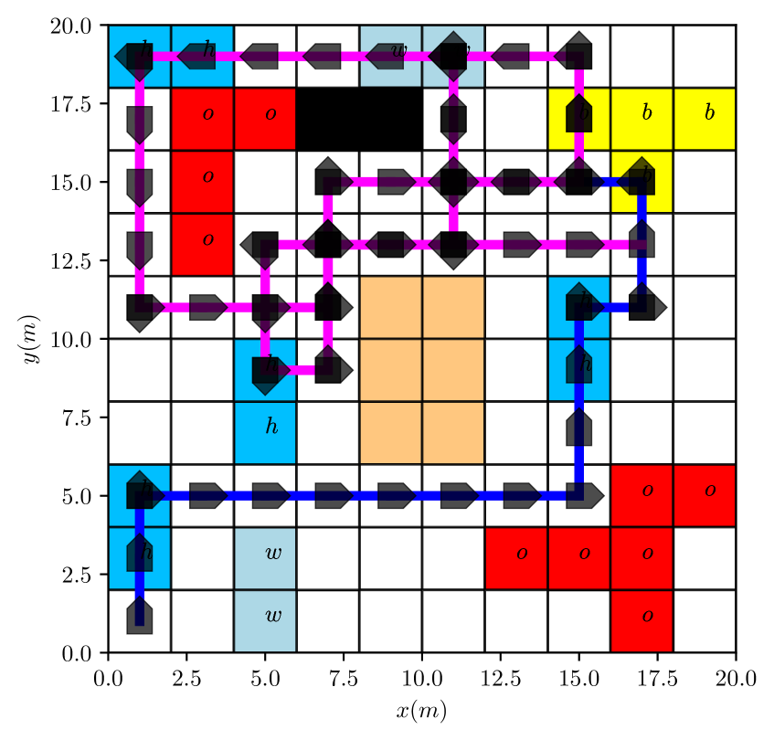
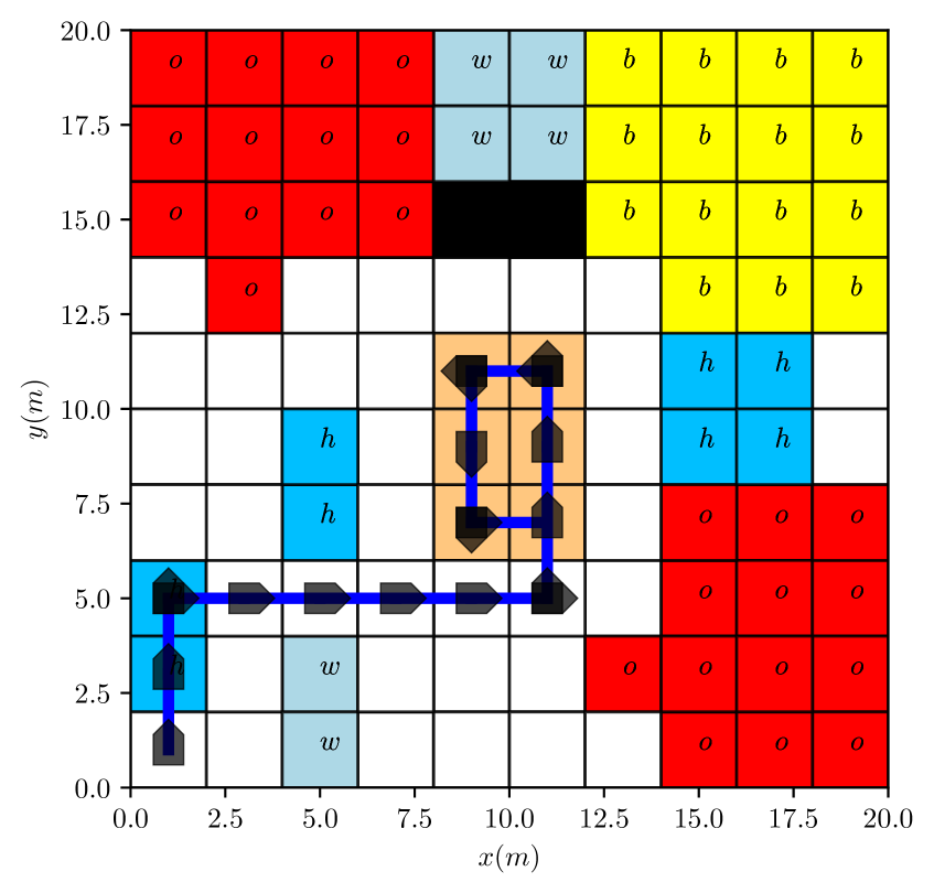
Figure 2: Sample trajectories under the proposed policy (left) and under the unsafe policy (right). Cells are marked by the features they satisfy, while valleys, hills are marked in brown and black.

V-B Simulation Results

The underlying MDP $\mathcal{M}$ has $400$ states and $3616$ edges and the DRA $\mathcal{A}_{\varphi}$ contains $21$ states, $111$ edges and one accepting pair. It took $5.7s$ to construct the resulting product $\mathcal{P}$ which has $8400$ states, $75936$ edges and one AMECs. We follow the policy synthesis and execution described in Sec. IV. When the system starts, the robot’s state is outside the AMEC. It took $0.01s$ to calculate the value function $v_{s}^{\star}$ via linear program [1] for the return policy. Then we formulate and solve (18) given $v_{s}^{\star}$ for the prefix synthesis in $0.02s$, which contains $2840$ variables and $712$ constraints. An optimal action is chosen based on plan prefix. Then the robot takes new measurements and updates $\mathcal{M}$ and $\mathcal{P}$ in a Bayesian way, which takes in average $1.5s$. This process repeats itself until the robot reaches the set of AMECs. Then the optimization (19) for the plan suffix is formulated (with $598$ variables and $1484$ constraints) and solved within $0.25s$. One sample trajectory is shown in Fig. 2, which satisfies the assigned search and rescue task. The trajectory prefix is marked in blue while the suffix is marked in magenta. It can also be seen that after the exploration and learning, the final workspace model is the same as the actual model. More importantly, due to the enforced safety constraint, the robot avoids during exploration the area of deep valley (in brown) and high hills (in black). In comparison, we also simulate the robot trajectory under the same synthesis algorithm but removing the safety constraints. One sample trajectory is shown in Fig. 2 where the robot remains trapped in the valley after time $9$. Thus it fails to satisfy the formula and leaves most of the workspace unexplored.

V-C Performance Evaluation

In order to further demonstrate the computational complexity of the proposed approach, we run $100$ Monte Carlo simulations of the above robotic system under different sizes of the underlying map, with similar setup of features. In Table I, we record the average synthesis time, the task satisfiability and the safety measure, which are compared with the approach that does not consider safety during exploration. First, it can be noticed that the proposed algorithm scales well with workspace size (with millions of edges in the last case). Constructing the product $\mathcal{P}$ takes considerable amount of time while solving the LPs associated with (18) and (19) are relatively fast. Second, it can be seen that both the task satisfiability and safety measure are greatly improved under the proposed approach. This is because in partially-known workspaces violating the safety constraint would also indicate the violation of assigned temporal task.

Approach	$\mathcal{P}$ Size	Time[$s$]		Safety	Satisfy
Proposed	(8.4e3,  7.6e4)	5.7	0.03	0.87	0.92
	(2.2e4,  2.1e5)	34	0.42	0.91	0.95
	(1.4e5,  1.4e6)	210	7.8	0.93	0.97
Unsafe	(8.4e3,  7.6e4)	5.7	0.01	0.1	0.3
	(2.2e4,  2.1e5)	30	0.31	0.2	0.25

Table I: Comparison of complexity and performance between the proposed and the unsafe approach. The “Time” column is split into the time to construct $\mathcal{P}$ and to synthesize $\boldsymbol{\pi}_{\texttt{o}}$. Note $a\texttt{e}b\triangleq a\times 10^{b}$.

VI Summary and Future Work

This work proposes a planning framework for robots operating in uncertain environments. The robotic task is specified as LTL formulas. During the learning and exploration, we enforce a safety constraint as the probability of returning to a set of home states during run time. The proposed approach fulfill both the temporal task and safety constraints. Future work includes the consideration of multi-robot systems.

References

• [1] M. H. Davis, Markov models and optimization.   Routledge, 2018.
• [2] X. Ding, S. L. Smith, C. Belta, and D. Rus, “Optimal control of markov decision processes with linear temporal logic constraints,” Automatic Control, IEEE Transactions on, vol. 59, no. 5, pp. 1244–1257, 2014.
• [3] K. Etessami, M. Kwiatkowska, M. Y. Vardi, and M. Yannakakis, “Multi-objective model checking of markov decision processes,” in Tools and Algorithms for the Construction and Analysis of Systems.   Springer, 2007, pp. 50–65.
• [4] C. Baier and J.-P. Katoen, Principles of model checking.   MIT press Cambridge, 2008.
• [5] V. Bruyere, E. Filiot, M. Randour, and J.-F. Raskin, “Meet your expectations with guarantees: Beyond worst-case synthesis in quantitative games,” Information and Computation, 2016.
• [6] M. Guo and M. M. Zavlanos, “Probabilistic motion planning under temporal tasks and soft constraints,” IEEE Transactions on Automatic Control, vol. 63, no. 12, pp. 4051–4066, 2018.
• [7] Y. Kantaros, S. Kalluraya, Q. Jin, and G. J. Pappas, “Perception-based temporal logic planning in uncertain semantic maps,” IEEE Transactions on Robotics, 2022.
• [8] X. Ding, M. Lazar, and C. Belta, “LTL receding horizon control for finite deterministic systems,” Automatica, vol. 50, no. 2, pp. 399–408, 2014.
• [9] A. Ahmed, P. Varakantham, M. Lowalekar, Y. Adulyasak, and P. Jaillet, “Sampling based approaches for minimizing regret in uncertain markov decision processes (mdps),” Journal of Artificial Intelligence Research, vol. 59, pp. 229–264, 2017.
• [10] M. Guo and D. V. Dimarogonas, “Multi-agent plan reconfiguration under local LTL specifications,” The International Journal of Robotics Research, vol. 34, no. 2, pp. 218–235, 2015.
• [11] J. Qian, R. Fruit, M. Pirotta, and A. Lazaric, “Exploration bonus for regret minimization in discrete and continuous average reward mdps,” Advances in Neural Information Processing Systems, vol. 32, 2019.
• [12] M. S. Talebi and O.-A. Maillard, “Variance-aware regret bounds for undiscounted reinforcement learning in mdps,” in Algorithmic Learning Theory.   PMLR, 2018, pp. 770–805.
• [13] J. Garcıa and F. Fernández, “A comprehensive survey on safe reinforcement learning,” Journal of Machine Learning Research, vol. 16, no. 1, pp. 1437–1480, 2015.
• [14] J. Klein, “ltl2dstar-LTL to deterministic streett and rabin automata,” http://www.ltl2dstar.de, 2007.
• [15] D. J. MacKay, Information theory, inference and learning algorithms.   Cambridge university press, 2003.
• [16] R. M. Neal, “Markov chain sampling methods for dirichlet process mixture models,” Journal of computational and graphical statistics, vol. 9, no. 2, pp. 249–265, 2000.
• [17] T. M. Moldovan and P. Abbeel, “Safe exploration in markov decision processes,” in 29th International Coference on Machine Learning.   ACM, 2012, pp. 1451–1458.
• [18] M. Guo and D. V. Dimarogonas, “Task and motion coordination for heterogeneous multiagent systems with loosely coupled local tasks,” IEEE Transactions on Automation Science and Engineering, vol. 14, no. 2, pp. 797–808, 2016.