Designing an Optimal Kilonova Search using DECam for Gravitational Wave Events

Abstract

We address the problem of optimally identifying all kilonovae detected via gravitational wave emission in the upcoming LIGO/Virgo/KAGRA observing run, O4, which is expected to be sensitive to a factor of $\sim 7$ more Binary Neutron Stars (BNS) alerts than previously. Electromagnetic follow-up of all but the brightest of these new events will require $>1$ meter telescopes, for which limited time is available. We present an optimized observing strategy for the DECam during O4. We base our study on simulations of gravitational wave events expected for O4 and wide-prior kilonova simulations. We derive the detectabilities of events for realistic observing conditions. We optimize our strategy for confirming a kilonova while minimizing telescope time. For a wide range of kilonova parameters, corresponding to a fainter kilonova compared to GW170817/AT2017gfo we find that, with this optimal strategy, the discovery probability for electromagnetic counterparts with the DECam is $\sim 80\%$ at the nominal BNS gravitational wave detection limit for O4 (190 Mpc), which corresponds to a $\sim 30\%$ improvement compared to the strategy adopted during the previous observing run. For more distant events ($\sim 330$ Mpc), we reach a $\sim 60\%$ probability of detection, a factor of $\sim 2$ increase. For a brighter kilonova model dominated by the blue component that reproduces the observations of GW170817/AT2017gfo, we find that we can reach $\sim 90\%$ probability of detection out to 330 Mpc, representing an increase of $\sim 20\%$, while also reducing the total telescope time required to follow-up events by $\sim 20\%$.

DES-2022-0714 FERMILAB-PUB-23-048-PPD

1 Introduction

The discovery of an electromagnetic (EM) counterpart to a gravitational wave (GW) event GW170817 ushered in a new era of astrophysics and multi-messenger astronomy (Abbott et al., 2017a; Soares-Santos et al., 2017; Cowperthwaite et al., 2017; Nicholl et al., 2017; Coulter et al., 2017b; Drout et al., 2017; Utsumi et al., 2017). The discovery of the optical counterpart occurred $\sim$12hr (Abbott et al., 2017b; Arcavi et al., 2017; Coulter et al., 2017a; Soares-Santos et al., 2017; Lipunov et al., 2017) after merger, allowing for extensive imaging and spectroscopic observations (e.g. Díaz et al., 2017; Andreoni et al., 2017; Balasubramanian et al., 2021; Kilpatrick et al., 2022). This enabled the community to not only confirm the existence of long-hypothesized kilonovae (KNe) and to characterize their lightcurves, but also to derive the first cosmological standard siren (Schutz, 1986) constraint (Abbott et al., 2017b).

The EM counterpart to GW1701817, AT2017gfo, was observed in $\gamma$-rays 2 seconds after the merger signal (e.g., Abbott et al., 2017; Goldstein et al., 2017; Savchenko et al., 2017), then a few hours later in optical bands as a fast-decaying blue object, with longer-lived emission in the infrared, X-ray, and radio bands. The astrophysics community is still learning from the vast data set compiled for this event. Early analyses showed that AT2017gfo had small ejecta masses with relativistic outflow velocities (from 0.1 to 0.3 of the speed of light $c$) and was likely powered by a combination of shocked material and r-process radioactive decay, which was modulated by the presence of high opacity lanthanides synthesized during the explosion and by a highly non-spherical ejecta and jet (e.g. Drout et al., 2017; Kasen et al., 2017; Thielemann et al., 2017; Gottlieb et al., 2018). Many questions about this event and the diversity of KNe remain open, including the dependency on the neutron star equation of state, the geometry of the ejecta, the nature of the early blue emission, the physics of the relativistic jet launch, the exact contribution of KNe to the r-process elements production, and the difference between KNe produced by binary neutron star (BNS) and neutron-star black-hole (NSBH) mergers.

The gravitational waveform observed from binary compact object mergers allow first-principles distance measurements. The GW distance measurement and the optical redshift of GW170817 provided constraints on the Hubble constant from a single event (Schutz, 1986; Del Pozzo, 2012; Abbott et al., 2017b), and further constraints came from measurements of $H_{0}$ from multiple GW events using a low precision statistical method (i.e dark sirens; Soares-Santos & Palmese et al. 2019; LIGO Scientific Collaboration & Virgo Collaboration 2019; Palmese et al. 2020, 2021; Finke et al. 2021; Gray et al. 2023).

From a cosmological perspective, the detection of GW170817 provided the grounds for the application of a new approach to understand the well-known Hubble tension. Measurements of the Hubble constant $H_{0}$ from early-time universe observations (e.g., Planck observations of the CMB in Planck Collaboration et al., 2020) are in tension with measurements from observations made at late times, e.g., the Hubble Space Telescope observations of Cepheids in concert with Supernovae as standard candles (Riess et al., 2021). These measurements have been made at increasing precision over the last few years, only adding to the open questions surrounding the tension; and thus have provoked a series of investigations of variations on the cosmological model (for survey papers, see, e.g., Knox & Millea, 2020; Schöneberg et al., 2022; Abdalla et al., 2022). There is no obvious resolution (Valentino et al., 2021), and the Hubble tension remains unresolved.

The GW distances measured from compact binary mergers do not rely on the distance ladder, and therefore will have different systematics than the astronomical distance ladder late-time measurements of $H_{0}$, and possibly smaller systematics. With additional standard siren measurements, the precision on the Hubble constant could reach the percent-level (Chen et al., 2018; Bom & Palmese, 2023). This level of precision would be an important contribution to resolving the Hubble tension (see discussion further below in this section).

The third LIGO/Virgo/KAGRA collaboration (LVK) observing run (O3) resulted in over 60 new events (see the third Gravitational-wave Transient Catalog, The LIGO Scientific Collaboration et al. (2021), hereafter GWTC-3). One GW event originated from a BNS merger and two high-confidence events originated from NSBH coalescences (Abbott et al., 2021), but no electromagnetic counterparts were confirmed from any event despite extensive follow-up campaigns (e.g., Morgan et al., 2020; Garcia et al., 2020; Tucker et al., 2022; Kilpatrick et al., 2021; Oates et al., 2021; Andreoni et al., 2019, 2019; Goldstein et al., 2019). One study (Graham et al., 2020) proposed an AGN counterpart to the binary black hole merger GW190521, but the association to the GW event cannot be made with confidence (Palmese et al., 2021; Ashton et al., 2020).

LVK’s O4 campaign is scheduled to start in early 2023, surveying on a factor of $2$ times more in the median Luminosity Distance and a factor of $\sim 7$ detections of BNS events than the previous O3 campaign (see table 2 in Petrov et al., 2022). The expected rates of BNS are uncertain but in the range of 9-88/year (Abbott et al., 2020; Petrov et al., 2022). It is unlikely that each subsequent KN event will obtain the same amount of follow-up resources as in O3. As GW detectors become more sensitive and able to detect events at larger distances, the optical follow-up of BNS events will become more challenging, including for campaigns using the Dark Energy Camera (DECam, Flaugher et al., 2015) such as those coordinated by the DES Gravitational Wave follow-up group (DESGW).

Here, we present improved and optimized strategies for discovery of KNe. The methodology presented here focuses on DECam resources, which the DESGW group plans to use to follow up LVK O4 events. However, the method is generic and could be easily adapted to any telescope. Our primary science goal is the construction of the standard siren Hubble diagram via maximizing the number of GW-detected events with known redshifts.

Our paper is structured as follows. In Section 2, we describe our GW and KN simulations. In Section 3, we discuss how we measure the success of each observing strategy. Section 4, we detail the various optimization options and types of KN models. In Section 5, we detail the strategies that we consider to be most successful for ensuring that DECam detects KNe with our follow-up observations. We additionally describe how this code may be used in a real-time follow up in Section 6. Finally, we discuss and summarize our results in sections 7 and 8.

2 Simulation Data

2.1 Simulated O4 BNS events

We start by producing a set of simulated BNS mergers that are expected to be detectable in the upcoming LVK O4 observing run. The procedure is similar to that in Petrov et al. (2022).

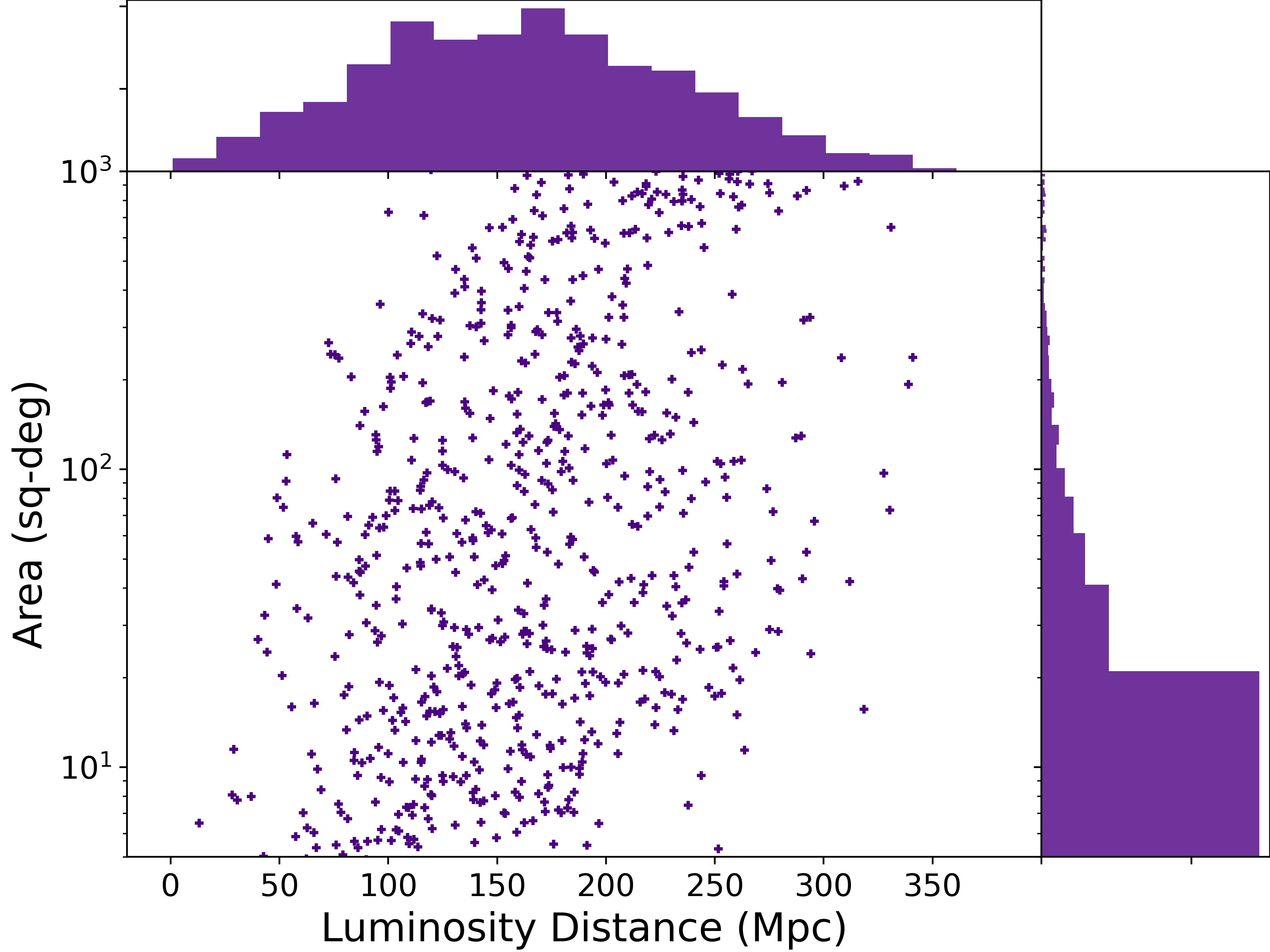
Figure 1: The distance distribution and $90\%$ credible interval sky localization area of the O4 simulations of BNS mergers used in this paper. The simulated primary masses follow a $\bar{x}=1.5M_{\odot},\,\sigma=1.1M_{\odot},\,x_{\mathrm{min}}=1.1M_{\odot},\,x_{\mathrm{max}}=3M_{\odot}$ Gaussian distribution, and the spins (see eq.(2) of first reference in The LIGO Scientific Collaboration et al. (2021)) of the events are distributed uniformly between $\pm$0.05. Simulated detections are limited to events with a network SNR greater than 12. Throughout the rest of this paper, we will assume follow-up of events only with area $<300$ degrees², which is 611 of the 860 events.

Figure 2: A sample of $10$ randomly chosen set of simulated Gravitational wave localization maps used in this work. The inner (outer) lines represents $\%50$ ($\%90$) confidence levels regions.

GW events are simulated using the BAYESTAR software (Singer & Price, 2016; Singer et al., 2016, 2016b), which uses LALSuite (LIGO Scientific Collaboration, 2018) tools. We assume sensitivity curves for Advanced LIGO, Virgo, and KAGRA as O4 sensitivities discussed in Abbott et al. (2020), though we assume a sensitivity for KAGRA of a BNS range of $\sim 80$ Mpc. All detectors have a duty cycle of 70%, which is consistent with LVK predictions Abbott et al. (2018). Assuming a Planck Collaboration et al. (2020) cosmology, we create $10,000$ BNS events of the type O4 could theoretically observe, following a uniform in comoving volume distribution, and then inject them into the GW Search and Discovery pipeline (Herner et al., 2020). TaylorF2 waveforms (Buonanno et al., 2009) are assumed both for injections and reconstructions. The primary mass distribution of our injections follow the neutron star mass function found in Abbott et al. (2021), normally distributed with mean 1.5 $M_{\odot}$ and standard deviation $1.1~{}M_{\odot}$, truncated to be within $1.1M_{\odot}\leq M_{\mathrm{NS}}\leq 3M_{\odot}$ in order to stay consistent with the Kasen models’ parameter space. The NS spin distribution was uniformly distributed between -0.05 and 0.05. After injecting the BNS mergers, a matched-filter search retrieves the detected events. We consider as detections those events for which a single–detector signal–to–noise ratio SNR$>4$ is reached by at least 2 detectors and the overall network SNR is $>12$, resulting in 860 detected events. The measured SNR is added with Gaussian noise. Finally, we produce BAYESTAR skymaps for the detected events. In Figure 1 we present the area (90% credible interval) and luminosity distance (integrated over the whole sky) for all of the simulations used in this analysis.

Petrov et al. (2022) argues that the alerts produced by the LVC during O3 are better modeled by dropping the two detector coincident detection requirement and using a minimum SNR for BNS events of $>8$. These criteria would have the effect of increasing the number of low SN, and therefore large sky area, events in our simulations. Figure 1 shows median luminosity distance of $\sim 150$ Mpc and sky area of $\sim 20$ sq-degrees, whereas Petrov et al. (2022) find $352\pm 10$ Mpc and $1820^{+190}_{-170}$ sq-degrees, a difference from previous work that they attribute to the changing of the SNR requirements. There are 249 from the total of 860 events that have 90% sky area $>300$ sq-degrees. To change our sample to have a median sky area of $\sim 350$ sq-degrees we would need an additional $\approx 360$ events, all of which would need $90\%$ sky area $>350$ sq-degrees. In our strategy definitions and proposed decision-making process to trigger limited Target-of-Opportunity resources, we choose a sky area limit of $<300$ sq-degrees, so we chose not to consider these additional high-sky-area events here. We do not make any other selections in the events.

2.2 Kilonova physical models

We model KNe using the time-evolving theoretical Spectra Energy Distributions (SEDs) of KN atmospheres from Kasen et al. (2017), hereafter referred to as the Kasen models. The Kasen models are parameterized by the mass ejected in the explosion, $M_{\mathrm{ej}}$, the abundance of lanthanide elements in the ejecta, $X_{\mathrm{lan}}$, and the velocity of the ejecta, $v_{\mathrm{ej}}$. The models are a set of $329$ time-dependent SEDs on a grid of discretized parameters: 0.001 M_$\odot$ $\leqslant$ $M_{\mathrm{ej}}$ $\leqslant$ 0.1 M_$\odot$, $0.03c\leqslant v_{\mathrm{ej}}\leqslant 0.3c$, and $1\times{10}^{-9}\leqslant{X}_{\mathrm{lan}}\leqslant 1\times{10}^{-1}$.

There are other KN models available in the literature (e.g. Bulla, 2019; Darbha & Kasen, 2020; Hotokezaka & Nakar, 2020; Wollaeger et al., 2021; Gillanders et al., 2022). In comparison to these, the Kasen models do not build in the dependence on the geometry of the mergers and the viewing angle (see, e.g., Stewart et al. 2022 for a visualization of an asymmetric KN supported by accretion disk simulations), but instead provide atmosphere models to be used in building a geometric model.

2.3 Kilonova lightcurve simulations

The lightcurve simulation pipeline is similar to that used Morgan et al. (2020), which constrains the physical KNe properties of GW190814. The SuperNova ANAlysis software (SNANA: Kessler et al. 2009, 2019) enables the simulation of light curves of KNe as they would be measured by DECam. SNANA produces light curves by simulating fluxes and uncertainties in observations by incorporating information about cadence, image zero points, and noise levels in search and template images. The light curves are in absolute magnitudes and are converted to observed magnitudes using a given cosmology. In particular, SNANA chooses a grid of 15 redshifts at $0.003\leqslant z\leqslant 0.2$, which is used to transform the Kasen model SEDs without evolution. The Kasen model SED is redshifted to a $z$ on our grid. SNANA also take into consideration the reddening by the dust in the Milky way (Kessler et al., 2019; O’Donnell, 1994). Later, the SEDs are convolved with DECam transmission curves accounting for atmosphere, telescope, filters, and CCDs. Given a cadence, the light curves are calculated by sampling the magnitude grid.

The $329$ Kasen models, $\alpha_{j}$, each with a range of time after burst, $\tau$ ($0.00\leqslant\tau\leqslant 16.7$ days), at the SNANA grid of redshifts, $z_{i}$ ($0.003\leqslant z\leqslant 0.2$), describe $829,080$ simulated magnitudes, $m_{\lambda}(\lambda,\tau,\alpha_{j},z_{i})$, for each of the 4 filters that we use ($g,r,i,z)$.

Table 1: Observational conditions (photometric filter, limiting magnitude, and effective exposure time) averaged from DECam follow-ups of previous observations. Note that the higher the $t_{\mathrm{eff}}$ value (which ranges from 0 to 1), the better the observational conditions.

Filter	$m_{0}$	$t_{\mathrm{eff}}$ (bright time)	$t_{\mathrm{eff}}$ (dark time)
$g$	23.4	0.05	0.7
$r$	23.1	0.15	0.8
$i$	22.5	0.45	0.7
$z$	21.8	0.6	0.6

2.4 DECam limiting magnitudes

We define the limiting magnitude as the magnitude at which we can measure a point source, e.g. a star, with $0.1$ mag error, which corresponds to signal-to-noise ratio, SNR $\sim 10$. We then define the limiting magnitude $m_{0}$ for a total effective exposure time of $90$ sec, i.e. $t_{\mathrm{exp}}\times t_{\mathrm{eff}}=90\mathrm{s}$, where $t_{\mathrm{eff}}$ is a unitless quantity that scales the exposure time to the ‘effective’ exposure time when taking into account sky conditions (higher $t_{\mathrm{eff}}$ being better sky conditions). Then, to scale up for different exposures, we construct:

$$m_{\mathrm{lim}}=m_{0}+1.25\log{\left(t_{\mathrm{eff}}\times\frac{t_{\mathrm{exp}}}{90\mathrm{s}}\right)},$$ (1)

which reflects S/N going as the square root of time in a sky noise limited observation. We use the $m_{0}$ measured in the DES data by Neilsen et al. (2016), thus the $90\mathrm{s}$ normalization factor, and present those values in Table 1, and the derived limiting magnitudes in Table 2. The $t_{\mathrm{eff}}$ is closely related to observational conditions during the night. Therefore, we break observing into nights of bright time and dark time and use $t_{\mathrm{eff}}$ from previous target of opportunity (ToO) programs in DECam, in particular the observations from past GW follow-up events (Morgan et al., 2020, Garcia et al., 2020). Although we split our tests into only dark and bright time, rather than on gray nights, which correspond to $\sim 50\%$ of the nights available in telescopes, we later show in Section 5.2, that the difference in performance between dark and bright and therefore gray is negligible due to the adaptability of the presented method. The differences are in the particular configurations chosen, e.g. the filters and exposures times selected in different observational conditions. Throughout this paper, we focus on detectability on dark nights unless otherwise stated.

Table 2: DECam $m_{\mathrm{lim}}(10\sigma)$, dark time

	Exposure time (sec)
Filter	$10$	$100$	$1200$	$3600$
g	22.0	23.3	24.6	25.2
r	21.8	23.0	24.4	25.0
i	21.1	22.4	23.7	24.3
z	20.3	21.6	22.9	23.5

Table 3: Observational parameter space $\Theta$ explored.

Time after burst (Days)	$0.5,1.0,1.5,2.0,2.5,3.0,3.5,4.0$
Scenario 1
Filter	$g,r,i,z$
2d credible sky area covered	$0.9,0.85,0.8,0.75,0.7$
Exposure time (sec)	$60,90,120,200,300,600,1200,3600$
Scenario 2 (with inner & outer region)
Filter	$g,r,i,z$
2d credible sky area covered
Outer: 0.9	Inner: $0.8,0.7,0.5,0.3$
Outer: 0.8	Inner: $0.7,0.5,0.3$
Outer: 0.7	Inner: $0.5,0.4,0.3$
Outer/inner exposure time pairs (sec)	60/90; 90/120; 120/200; 200/300;
	300/600;  300/1200; 600/1200;  600/2400;
	1200/2400; 2400/3600; 3600/5400

2.5 Cadences & observational parameters

We use of SNANA to find effective search strategies that maximize candidate detection, considering realistic conditions, including the maximum duration of the night, intervals between observations, and sky brightness, while also minimizing telescope time and enabling earlier discovery. This is at base a trade-off of exposure times versus sky area coverage, but with additional complications of filter choice and the time since the event occurred. We limit our telescope time expenditures to $8$ hours per night and assume Blanco/DECam has telescope/readout slew time of $30\mathrm{s}$ between the exposures, which is true for small slews, such as the ones less than $\sim$ 10 degrees. In fact, long slews $\sim 100$ deg, which might be necessary to cover disjoint gravitational wave maps, take on the order of $3$ minutes. Thus, if there are two disjoint regions, which would add one or possibly two long slews depending on the observational conditions, it would add a negligible amount of total telescope time, relatively. We test four filters, $g,\,r,\,i,\,\mathrm{and}\,z$, starting $12$ hours after the trigger, and going to 4 days post-merger in half-day increments with several exposure times. These are summarized in Table 3.

Note that the time required to respond a GW alert depends upon several factors including human decision-making to trigger, when the event is visible in the sky, observation planning, and time to ask for and obtain the ToO interrupt. The time required to get the telescope on-sky also depends on when the alert is given. It is possible that it may be significantly less than 12 hours until we are on-sky, however, for this study we opted for a conservative option of 12 hours, by which time for any significant and observable event we should be able to observe.

We define two exposure time scenarios. In Scenario 1 we cover the area of a given GW event with a single set of exposure times and in Scenario 2, we explore the use of two different exposure times for a single search. The latter is motivated by the need to cover the high probability area sky with deep exposures, while covering the larger low probability localization area outskirts with shorter exposure images. We designate central high probability areas as the “inner region” and the rest of the area inside the the localization region as the “outer region”. The last section of Table 3 presents the combinations considered for the inner region, ranging from $30\%$ to $80\%$ sky probability coverage, for 3 different values of the total (deep+shallow) sky map probability coverage, from 70% to 90%. For instance, a combination of $40\%$ probability for the inner region and $70\%$ total coverage means that the $40\%$ highest probability region is covered with higher exposure time and the $70-40=30\%$ left over is covered with the shorter exposures. Each of these combinations is considered for all possible deep and shallow exposures presented in Table 3. For scenarios where we cover the sky area twice in a single night, we additionally take into consideration the KN variability a few hours after the first search.

2.6 Simulation data summary

We simulate a set of GW detections $S={S_{1},\ldots,S_{n}}$, where $n=611$ and $S_{i}$ is the $i^{th}$ simulation with distance $d_{i}$. For each $S_{i}$ we evaluate each of the parameter sets $\Theta$ in the two scenarios. In Scenario 1 there are 8 passes since burst, 4 filters, 8 exposure times, and 5 sky area probability coverages: $8\cdot 4\cdot 8\cdot 5=1280$ possible parameter sets. In Scenario 2 there are $8\cdot 4\cdot 11\cdot 10=3520$ possible parameter sets to be evaluated. Over both, 4800 observation models are evaluated. Each model is evaluated with the machinery described in Section 2, resulting in SNANA kilonova measured magnitudes. We have done this for each of the 329 Kasen models.

3 Detection Methodology

3.1 Discovery probability

We define the probability of detection, $p_{\alpha_{j}}$, of the KN model $\alpha_{j}$ for the $j^{th}$ combination of $(M_{\mathrm{ej}},\log(X_{\mathrm{lan}}),v_{\mathrm{ej}})$, with observed magnitude $m_{\lambda}=m(\lambda,\tau,\alpha_{j},z_{i})$ in a given filter $\lambda$, for a given exposure time $t_{\mathrm{exp}}$ weighted by observing condition $t_{\mathrm{eff}}$  for an event at mean redshift, $\bar{z}$, over the SNANA grid of redshifts, $z_{i}$:

$$p_{\alpha_{j}} \propto\sum_{i}\begin{cases}pr(\alpha_{j})\cdot pr(z_{i}),&\text{if}\,\mathrm{m}_{\lambda}<\mathrm{m}_{\mathrm{lim}}\\ 0,&\text{if}\,\mathrm{m}_{\lambda}\geq\mathrm{m}_{\mathrm{lim}}\end{cases}\,$$ (2)

$$\mathrm{where}$$

$$\alpha_{j} \equiv j^{th}\mathrm{\,combination\,of\,}(M_{\mathrm{ej}},\log(X_{\mathrm{lan}}),v_{\mathrm{ej}}),$$

$$p_{\alpha_{j}} \equiv p_{\alpha_{j}}(\mathrm{detection}|\tau,t_{\mathrm{eff}},\Theta,\bar{z}),$$

$$\mathrm{m}_{\lambda} \equiv\mathrm{mag}_{\lambda}(\lambda,\tau,\alpha_{j},z_{i}),$$

$$\mathrm{m}_{\mathrm{lim}} \equiv\mathrm{mag}_{\mathrm{lim}}(\lambda,t_{\mathrm{eff}},\Theta),\quad\mathrm{and}$$

$$pr(z_{i}) =\exp\left(-\frac{(z_{i}-\bar{z})^{2}}{2\sigma_{\bar{z}}^{2}}\right),$$

where $\tau$ is time after the GW detection, $\Theta$ contains the specific observation strategy characteristics including $t_{\mathrm{exp}}$, filter and area coverage as described in Table 3, $\mathrm{m}_{\mathrm{lim}}$ is the limiting magnitude of the observation for a $10\sigma$ detection, and $pr(\alpha_{j})$ are the model priors defined by each kilonova model described in the Section 4.2 and Table 4. The summation is over all redshifts for a given model, $j$ at a given $\tau$. Eq. 2 represents a Gaussian prior for choosing light curve models from the grid of SNANA defined redshifts given the GW distance. Explaining it differently, Eq. 2 is, for a given Kasen model, examining whether the resulting apparent magnitude is less than the limiting model with a Gaussian prior on the redshift, using the GW event mean redshift, $\bar{z}$, and the grid of SNANA redshifts the KN could be at, weighted by the GW event variance in redshift, $\sigma_{\bar{z}}^{2}$.

The GW localization maps present the probability that the event is located at a given sky position, the luminosity distance at that position and its uncertainty. Therefore we define the total probability of detecting an event as

$$P_{d} =\frac{\int_{\hat{\Omega}}d\Omega\,\,d_{L}(\Omega)\,p(\Omega)}{\int_{\hat{\Omega}}d\Omega\,\,d_{L}(\Omega)}\,\times\sum_{j=1}^{329}p_{\alpha_{j}}\,,$$ (3)

$$\mathrm{where}$$

$$P_{d} \equiv P(\mathrm{discovery}|\hat{\Omega},\tau,t_{\mathrm{eff}},\Theta,\bar{z})$$

and $\hat{\Omega}$ is the entire sky area observed in the follow-up, the $d\Omega$ is the voxel, $p(\Omega)$ is the probability in the voxel, and $d_{L}({d\Omega})$ is the luminosity distance to the voxel. The sum over $p_{\alpha_{j}}$ includes the priors and thus indicates the model used. The sky coverage and exposure times determine the total telescope time for a given KN detection. We note that we use weighted spatial probability, rather than 2-d on-sky probabilities, therefore we have the $d_{L}$ weighting in Eq 3.2 and the attendant implication that we can have a higher detection probability than on-sky credible area covered. We can now evaluate $P_{d}$ for a given set of $\Theta$.

3.2 Confirmation probability

In order for an object to be confirmed as a kilonova candidate, we require it be detected twice (in two observing ‘epochs’). This requirement can be lifted if, for example, there are sufficient spectroscopic resources available to follow-up all of the candidates found after a single epoch. Generally this is not the case, however. The second detection eliminates spurious detections, including image artifacts, asteroids and other possible contaminants (Morgan et al., 2020; Shandonay et al., 2022). Another reason to consider the detections independent is that we typically observe while working on post-processing and making target selection for spectroscopy in the data from the previous epoch.

Given that we want to make two detections to positively identify kilonova candidates, we define the probability of confirming the transient with two independent detections as:

$$P_{c}\equiv P(\mathrm{confirmed})= P(\mathrm{discovery}|\hat{\Omega},\tau_{1},t_{\mathrm{eff}},\Theta,\bar{z})$$ (4)

$$\times P(\mathrm{discovery}|\tau_{2},t_{\mathrm{eff}},\Theta,\bar{z})$$

where,

$$P(\mathrm{discovery}|\tau,t_{\mathrm{eff}},\Theta,\bar{z})=\sum_{\alpha_{j}}p_{\alpha_{j}}.$$

We design the strategies along the paper optimizing for $P_{c}$ given a set of constraints. Due to implementation choices and to speed up the numerical optimization we use $P_{c}^{\star}\equiv P_{d,1}\cdot P_{d,2}$ which gives us equivalent results in terms of strategy  such as telescope time or the duration of the night. We further present our main findings as a function of discovery probability, which is the most relevant outcome for the proposed strategies.

4 Optimizations and Kilonova Types

After calculating $P_{c}$ for each O4 event in two observing scenarios each with a grid of observational parameters we can evaluate what works best to optically find the kilonova. The answer to this depends on the science goal. Our primary science objective is standard siren cosmology, so we aim to identify optical counterparts to every kilonova-progenitor detected by the LVK. To this end, we chose to focus on optimizations that require two detections at least 30 minutes apart, in order to remove spurious detections due to asteroids. In this section we discuss the optimizing the strategy given the science goal, and then discuss the detailed metric, which involves exploring the meaning of covering the space of Kasen models.

4.1 Optimizations

We derive $P_{c}$ for each of the 1280 parameter combinations of Scenario 1 and for each of the 3520 combinations of Scenario 2, resulting in 4800 total for each simulated merger detection event, $S_{i}$. Not all of these combinations have an appreciable $P_{c}$ much above zero, as most of the predicted magnitudes are below sky noise.

We use $P_{c}$ as the variable to optimize on. We choose the highest $P_{c}$ for each sim $S_{i}$, look up the set of observational parameters $\Theta_{i}$ for it, and define this the Top strategy. Choosing the highest $P_{c}$ is the simplest optimization, but for our evaluation we need at least two more, Reference and Low Telescope Time.

1. Top Strategy is the $\Theta_{i}$ producing the highest $P_{c}$ for each $S_{i}$, the observational parameters producing the highest probability of confirmation for every O4 simulation.

2. Low Telescope Time (low-TT) is the $\Theta_{i}$ combination that uses the lowest telescope time given while retaining a $P_{c}$ within 10% of the highest confirmation probability strategy, by definition Top. For example, if the Top strategy finds $P_{c}=0.85$, then a low-TT strategy will have $P_{c}\geq 0.75$, usually with a much reduced telescope time. We will find it interesting to vary the threshold away from $10\%$.

3. Reference Strategy has the 90$\%$ probability sky area observed in $i$ and $z$ bands with 90 second exposures on the first two nights after the merger. This strategy models previous DECam searches, in particular the extensive search of Morgan et al. (2020), and has been used as the DECam strategy for the predictions of Chase et al. (2022).

The Top strategy uses as much telescope time as possible to explore the volume, given the parameter exploration presented in Table 3. All strategies work within the constraint of requiring two passes over two 8 hour nights.

4.2 Bayesian Average Models

Table 4: Kilonova Gaussian model priors.

	Blue & Bright		Reddish & Slow		Red & Faint
	$\mu$	$\sigma$	$\mu$	$\sigma$	$\mu$	$\sigma$
$M_{\mathrm{ej}}(M\textsubscript{$\odot$})$	0.025	0.001	0.025	0.01	0.035	0.15
$\log(X_{lan})$	-5.0	1.0	-5.0	10.0	-2.0	5.0
$v_{\mathrm{ej}}$ ($c$)	0.25	0.01	0.25	0.10	0.15	0.30
Peak $\left<M_{i}\right>$	$-16.3$		$-15.7$		$-14.6$

Not every Kasen model atmosphere is equally likely to be a good model for a real KN light curve. Most models for GW170817 are 2+ component models, as in Kilpatrick et al. (2017); Villar et al. (2017); Coughlin et al. (2018); Gillanders et al. (2022). If the Kasen models define a linear space of KN models, then the Kilpatrick models are in that space; if the Kasen models are eigenmodels of KN, then the models in Kilpatrick et al are defined by the eigenvalues multiplying the eigenmodels. Both the values of the non-zero eigenvalues and the number of non-zero eigenvalues are highly model dependent. Dropping the eigenvector language, it is clear that in the current situation of very few well studied KNe, the number of components in models describing KNe candidates is uncertain.

One of the most common ways to define detection efficiency in the literature is to set up a grid of KN models, for example over viewing angle, as done for a $\chi^{2}$ analysis and then calculating the fraction of models detected given an observation. This makes the detection probability explicitly dependent on non-physical choices of the grid breadth and grid spacing. In our case the grid would be the 329 Kasen models, even though these models were meant to extend past the range of models likely to describe real KN. In a Bayesian framework, each of these models would come with a prior describing our belief in their applicability.

We will employ the useful idea of a Bayesian model average. We evaluating the entire grid of Kasen models, but instead of a uniform weighting we place a Bayesian prior, $pr(\alpha)$, on each model. The Bayesian average model detection probability is implicit in eq 2, but can be thought of as:

$$\left<P_{d}\right>=\sum_{j=1}^{329}\,P_{d}\cdot\,pr(\alpha_{j})$$ (5)

where $\sum pr(\alpha_{j})=1$. Here we will use Gaussian priors to produce three Bayesian average models, bright & blue, reddish & slow, & red & faint, as given in Table 4. It is useful to guide the intuition to form the Bayesian average model absolute magnitude,

$$M_{\lambda}(\lambda,\tau)=\sum_{j=1}^{329}\,M_{\alpha_{j}}(\lambda,\tau,\alpha_{j})\cdot\,pr(\alpha_{j})\,,$$ (6)

of which peak $M_{i}$ is also given in Table 4 and light curves shown in Fig 3. This mean quantity, while illuminating, is incomplete as the Bayesian formalism is designed to make the uncertainties explicit- the curves are to thought of as the median value of a band of light curves weighted by the prior.

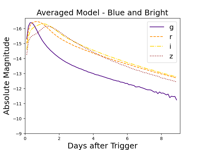
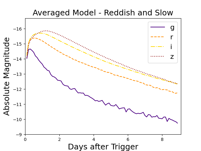
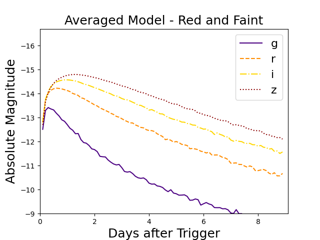
Figure 3: The absolute magnitudes $x$ days after the trigger for the weighted average of three sets of priors in the KNe parameter space models considered.

The bright & blue model is defined as the means and uncertainties of the blue component model in Kilpatrick et al. (2017) interpreted as Gaussian priors. Since Kilpatrick et al. (2017) gives no uncertainties for the blue model, we assume for $M_{\mathrm{ej}}$ a relatively narrow 0.001, and for $v_{\mathrm{ej}}$ of 0.01. Where Kilpatrick et al. (2017) has the blue model lanthanide fraction evolving from $\log{X_{\mathrm{lan}}}=-4$ to -6 as the opacity falls due to KN atmosphere expansion, we take $\log{X_{\mathrm{lan}}}=-5$ with an uncertainty of 1.0. This model is, in average, blue and reaches a peak luminosity a half day after trigger in $g$-band. It is also, in average, the brightest of the three models and $0.8$ magnitudes brighter than GW170817’s peak $M_{g,r,i,z}\approx-15.5$.

The reddish & slow model is defined as in bright & blue, except that we take the $\sigma$ to be ten times the uncertainties there, to reflect our ignorance of the KNe population. This results in a prior allowing the entire $\log{X_{\mathrm{lan}}}$ range of the Kasen models to contribute. Such wide priors make our model, in average, to be redder and slower to peak than GW170817, though with the same $\left<M_{i}\right>$. Most of our results use this model.

The red & faint model is defined as the means and ten times the uncertainties of the red component model in Kilpatrick et al. (2017) interpreted as Gaussian priors. The predominantly lanthanide-rich Kasen models contribute. This results in a model that is, in average, redder and fainter than GW170817, with a peak $\left<M_{i}\right>$ fainter by 1 magnitude, and a $\left<M_{r}\right>$ fainter by 1.4 magnitudes. This model aligns with what is expected by most models for viewing KN in the orbital plane, where the lanthanide-poor material is hidden from view.

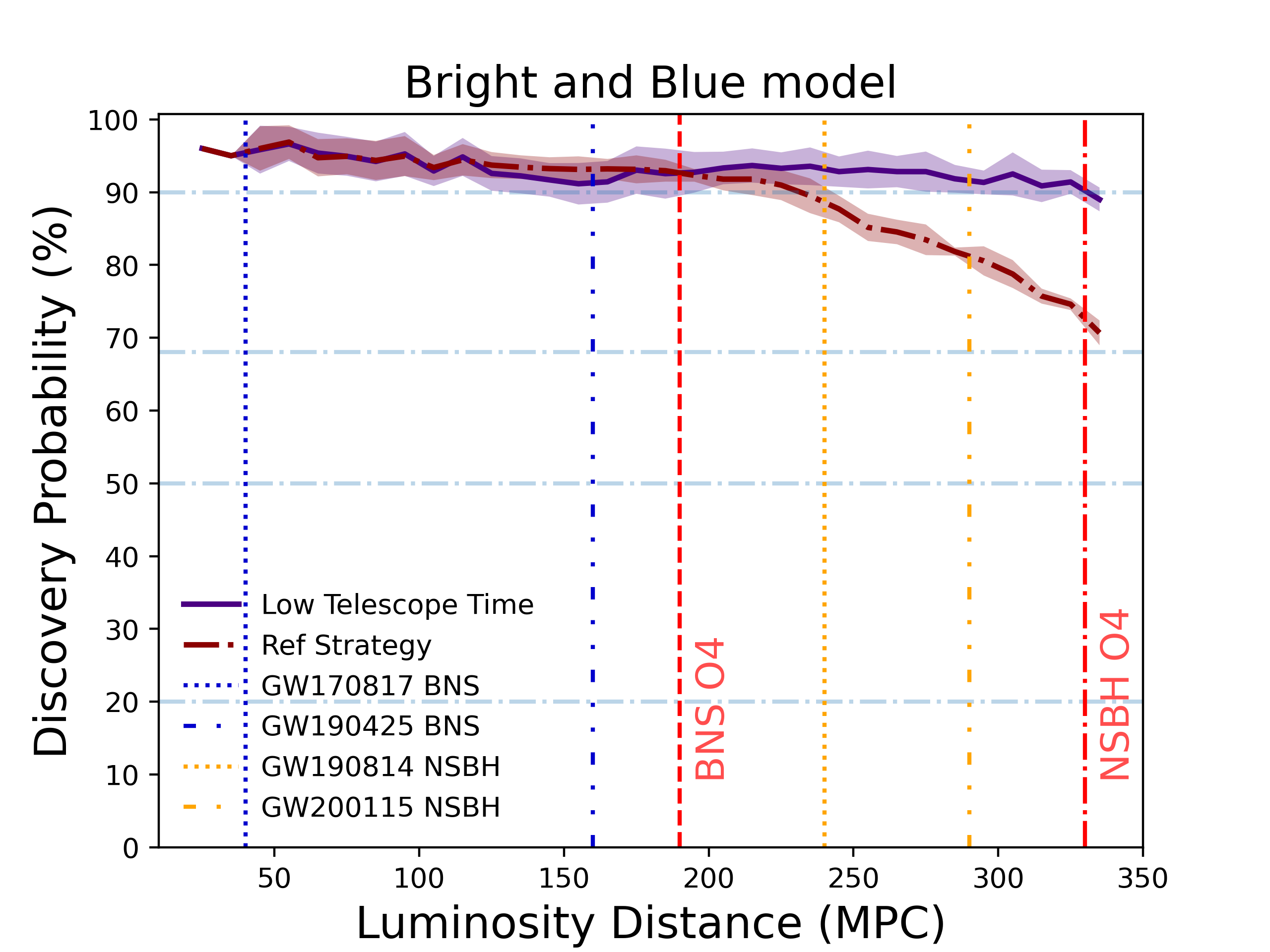
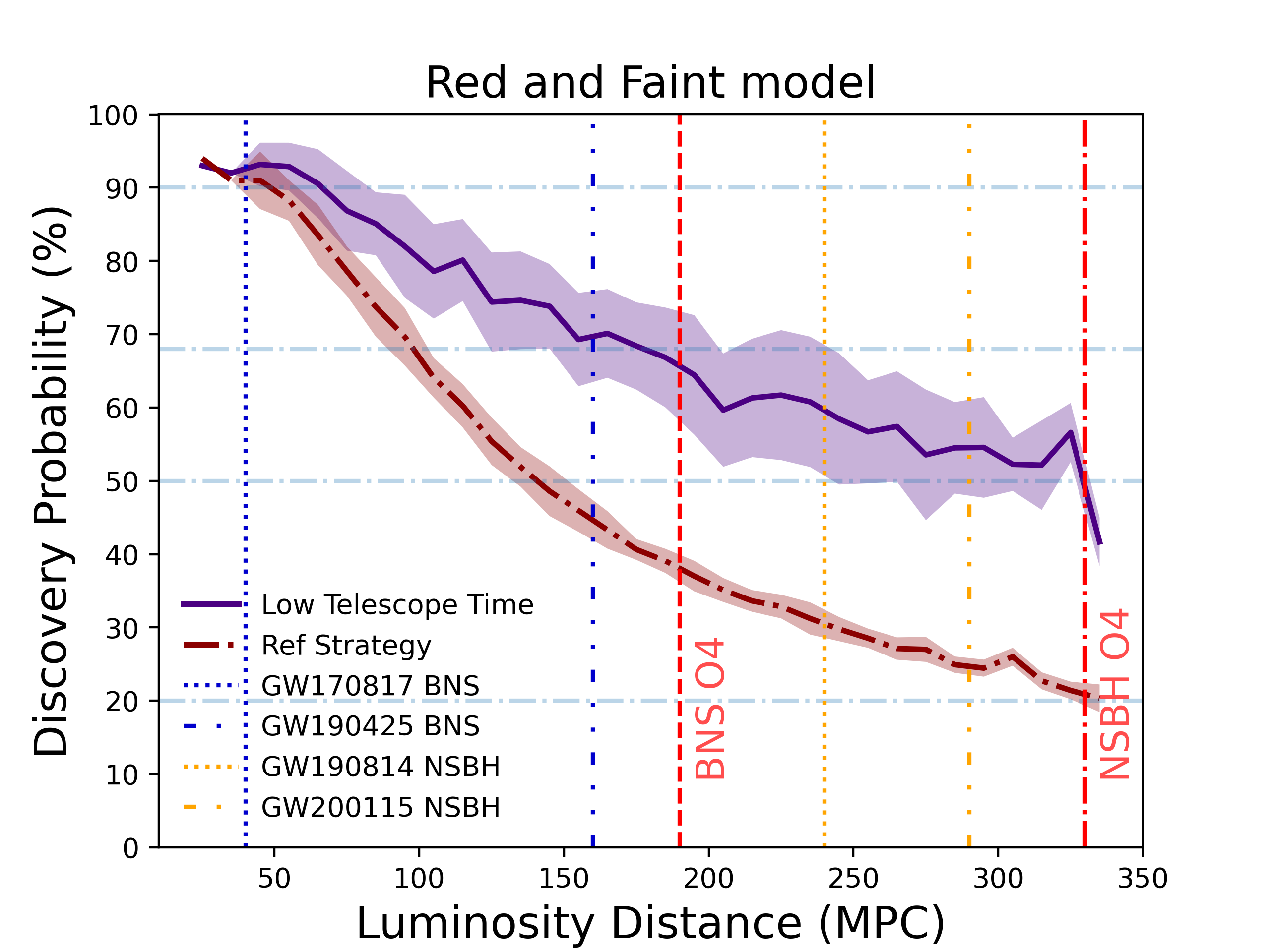
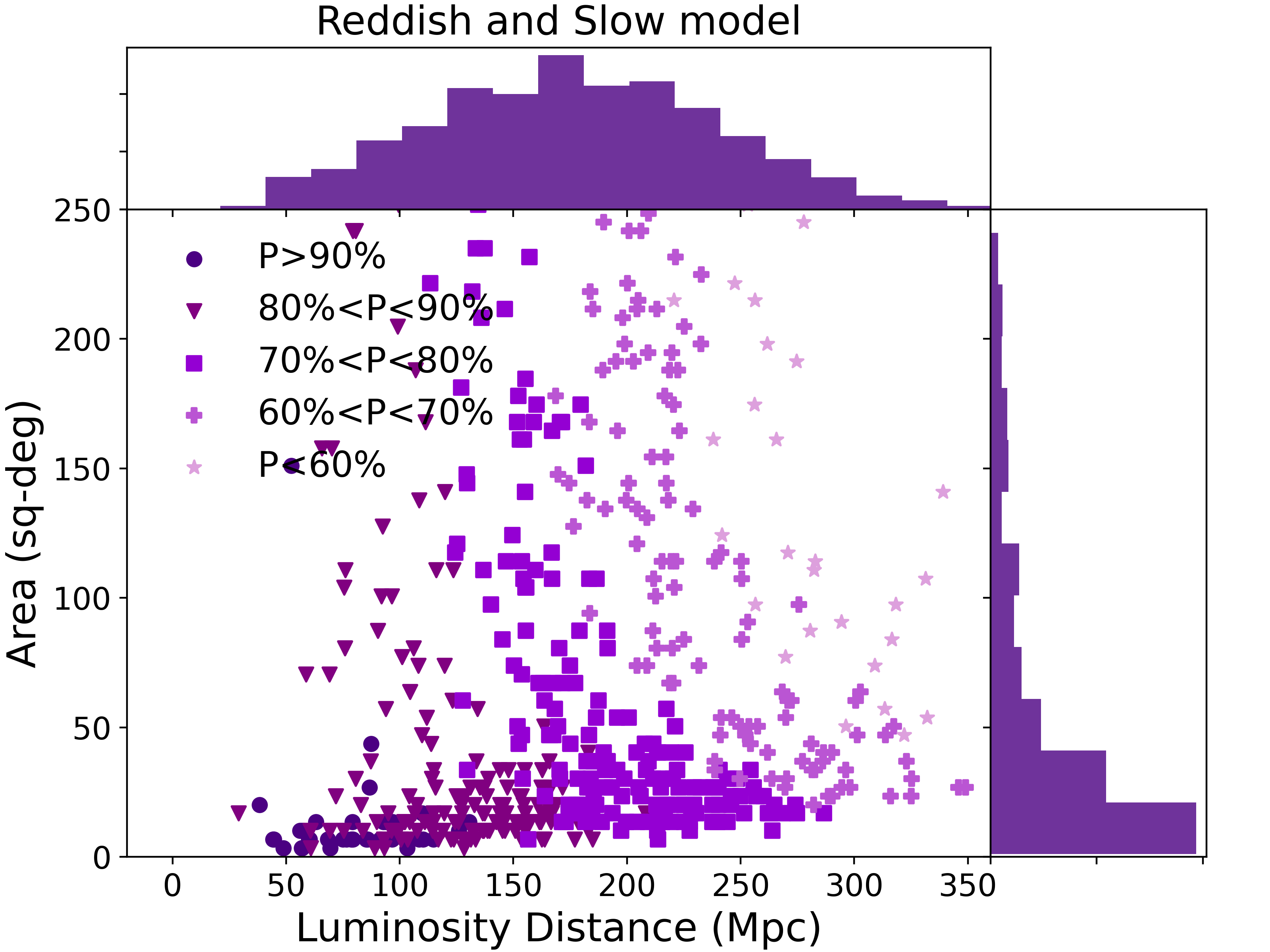
Figure 4: Discovery probability vs luminosity distance using the low-TT observing strategy compared to the Ref strategy for the 611 events with $90\%$ probability area $<300$. Each plot describes a different KNe model where (Upper Left:) bright & blue, (Upper Right:) reddish & slow, (Bottom Left:) red & faint. The shaded region about the median line represents the $68\%$ confidence interval of the scatter among the simulations. We also mark the distance to the upper limit of the LVK O4 projected range as well as noted GW events for reference. Bottom Right: distribution of simulations with for the low-TT strategy, binned by discovery probability in our wide prior model, reddish & slow. The marginal histograms are discovery weighted.

We will use our three models in various ways to evaluate the optimized strategies. The bright & blue model will be the easiest to detect, as the light curves peak brighter than $-16$ in $g,r,i,z$. The red & faint model will be the hardest, as the absolute magnitude peaks only brighter than $-13$ in $g$, barely $-14$ for $r$, approaching $-15$ for the the observationally more difficult $i,z$. The reddish & slow model is intermediate. In this paper, we often use bright & blue to inform the reader’s intuition to low inclination angle KN. We use red & faint to show the effect of a faint KN on the strategies. It can be argued that the red & faint represents the most likely KN from a NSBH merger, as those events are expected to be redder and with low absolute luminosity compared to NSNS mergers (Anand et al., 2021). We often use reddish & slow as an intermediate case that shows the behavior of choices in strategy optimization well.

There remains considerable uncertainty in the KN population statistics. While our three models are comparable to those in, e.g., Zhu et al. (2023); Sagués Carracedo et al. (2021); Coughlin et al. (2020); Petrov et al. (2022), the population study of Setzer et al. (2022) has a two peaked absolute magnitude distribution, at $i$-band absolute magnitudes of $-15$ and $-12$. In that study, GW170817 is a $95^{th}$ percentile event in luminosity, and the $50^{th}$ percentile luminosity corresponds to our $\left<M_{i}\right>$ for red & faint. The Setzer et al. (2022) study is for a random distribution of inclination angles and thus corresponds to the intrinsic KN population, whereas it is known that GW observatories predominately select merging compact objects with inclination angles near $\approx 30^{circ}$ (see, e.g., Finn & Chernoff, 1993; Nissanke et al., 2010; Schutz, 2011). The observed KN population from GW event followup will mostly be from the first peak of Setzer et al. While a KN sample with $M\approx-12$ would be challenging even for a 4m telescope, the first peak $M\approx-15$ is inside our model ranges.

We take our priors from Kilpatrick et al. (2017) because we wish to emphasize the uncertainties in the models in this study. The uncertainties in the models reported by Villar et al. (2017), for example, are much smaller. For observations in O4 the models and uncertainties in Coughlin et al. (2018) are likely more accurate and constraining for GW170717. However, we prefer to keep a wide variety of possible KNe. We suggest using the 2-component lightcurve red and blue models as the counterparts to our bright & blue and red & faint models, interpreted as a low and large inclination angle models and to use the 1-component model with $10\sigma$ as the counterpart to our reddish & slow, interpreted as a maximally uncertain KN population model.

4.3 Strategies and KN models

We begin our study of the strategies. As the community routinely uses the probability of detecting a KN once, calling this discovery, we will be showing $P_{d}\equiv P_{d,1}$ in most of the succeeding plots. Note that the strategies are all optimized on $P_{c}$ and in our language, “chance of discovery” is to be interpreted as “fraction of models detected given our priors on the space of models”.

Reducing our GW population population statistics to only distance, we can describe the NS-NS merger population in Figure 1 as having a median $d_{L}$ of 150 Mpc, a $75\%$-tile of 225 Mpc, and having only $1\%$ at $d_{L}>300$ Mpc. We take 200 Mpc as a characteristic distance.

We show in Figure 4 the low-TT strategy discovery probability as a function of distance and compare it to the reference strategy. Starting with the easy case model, bright & blue, we see that the low-TT detection probability has a ceiling at $\approx 90\%$. The reference strategy $P_{d}$ falls after 200 Mpc, whereas the low-TT $P_{d}$ remains high out to 330 Mpc. The red & faint model is difficult for the reference strategy after about 100 Mpc, whereas the low-TT has $P_{d}>50\%$ out to 330 Mpc. The reddish & slow model is intermediate and the low-TT performs well. The luminosity distance vs area distribution shows the probability weighted histograms on the margins. Not surprisingly, small spatial localizations are both are easiest to make identifications for, but less obvious is that the most likely distances for detection is flat between 125 Mpc and 175 Mpc.

The exposure time must be balanced by the sky area to be covered: in our maximum 8 hours per night DECam using 1 hour exposures can survey 24 square degrees per night. Figure 1 shows that the number of events with sky area less than 24 square degrees drops rapidly at distances greater than 200 Mpc.

Turning to the the distribution of telescope time required per event in Figure 4, we will explore the motivation and design of the low-TT strategy. For the best (by construction) $P_{c}$ strategy Top  the mode of the time required is $\approx 13-15$ hours for reddish & slow & red & faint, but saturates at $3-5$ hours for bright & blue. The Top strategy likes to use all the time available over two nights to maximize detection. The low-TT strategy is the lowest telescope time within 10% of Top’s $P_{c}$, but clearly one can tune how much loss in $P_{c}$ one is willing to accept. We have compared choosing $5\%$,$10\%$ and $15\%$ (see Table 5) and not surprisingly the best choice depends on the KN model chosen. For the bright & blue model, a threshold of $5\%$ gives a strategy that outperforms the Reference strategy in $P_{d}$, in particular after 200 MPc, while using less total telescope time considering following up $90\%-100\%$ of the best-localized events after our initial cut of $300$ sq degrees. This is, in fact, one of the key advantages of our proposed method: we scale up the exposure times with the distance while the Reference strategy keeps the same exposure times of $90s$, thus we keep high performance in farther away events and use only the necessary time for close events. Another critical point to make optimized use of time is the fact that our proposed method allows the use of shallower exposures in the outer regions that contain less probability, while focusing more deep exposures in the core probability region. This configuration, named scenario 2 in Table 3, was preferred as discussed later in the Section and is the one presented in the plots unless otherwise stated. This is particularly important in low-TT strategy, since it selects, most of the time, $60$s exposures in bright & blue model in the outer regions and therefore saves time compared to Reference. For the reddish & slow and red & faint models, we prefer to set the threshold at 10%. This produces in the reddish & slow case a strategy that uses a factor of 3 less telescope time than Top, and the red & faint case a factor of 2 less, for a loss in $P_{c}<10\%$. The gain in $P_{d}$ over the reference strategy is particularly dramatic for red & faint at higher distances.

Table 5: Average telescope time per event in hours required for two detections, discovery and confirmation. The events used were all that had $90\%$ probability area $<300$ sq-deg. From 860 events, 611 are retained after this cut. The $50\%$, $90\%$ or $100\%$ columns give average times for events ordered by the statistics of the size of the $90\%$ localization area, low to high.

Strategy	Telescope time (hours)
bright & blue	$50\%$	$90\%$	$100\%$
Reference	0.4	1.1	1.6
Top	2.3	3.0	3.2
low-TT ($5\%$)	0.4	0.9	1.3
low-TT ($10\%$)	0.4	0.9	1.2
low-TT ($15\%$)	0.2	0.7	0.9
wide prior, reddish & slow
Reference	0.4	1.1	1.5
Top	10.5	12.1	12.2
low-TT  ($5\%$)	5.2	6.8	7.0
low-TT  ($10\%$)	3.2	4.3	4.5
low-TT  ($15\%$)	2.2	3.0	3.2
red & faint
Reference	0.4	1.1	1.6
Top	10.4	12.3	12.6
low-TT  ($5\%$)	7.4	9.1	9.2
low-TT  ($10\%$)	5.4	6.3	6.4
low-TT  ($15\%$)	4.1	4.8	4.8

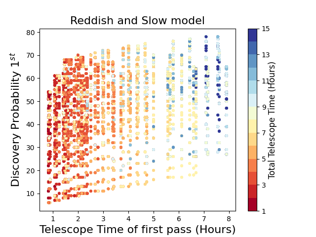
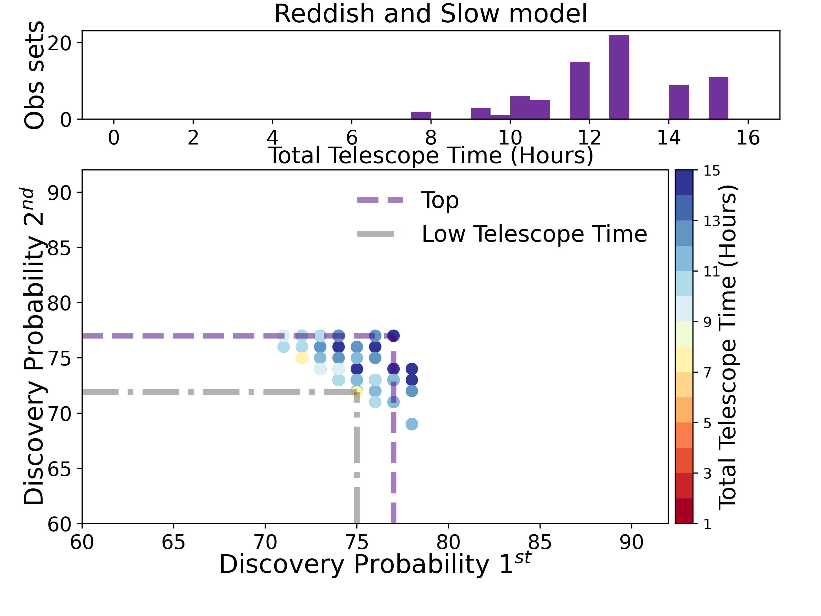
Figure 5: Discovery propabilities of diferent $\Theta_{i}$ sets of configurations on a single event in scenario 2. The event is located at 160 Mpc with $90\%$ sky area of 168 sq-degrees in a reddish & slow kilonova model peaking at $0.9$ days after the burst in $i$ and $1.2$ in $z$ Upper: Discovery probability vs time to completion of first pass denoted for each configuration $\Theta_{i}$. Total telescope time in hours is color coded. Bottom: The best 10% of Confirmation Probability from the upper plot, displayed in a $P_{d,1}$ vs $P_{d,2}$ plot with total telescope time color coded. The $\Theta_{i}$ corresponding to Top and low-TT strategies are marked. The histogram gives the distribution of telescope times for the $\Theta_{i}$ in the lower plot.

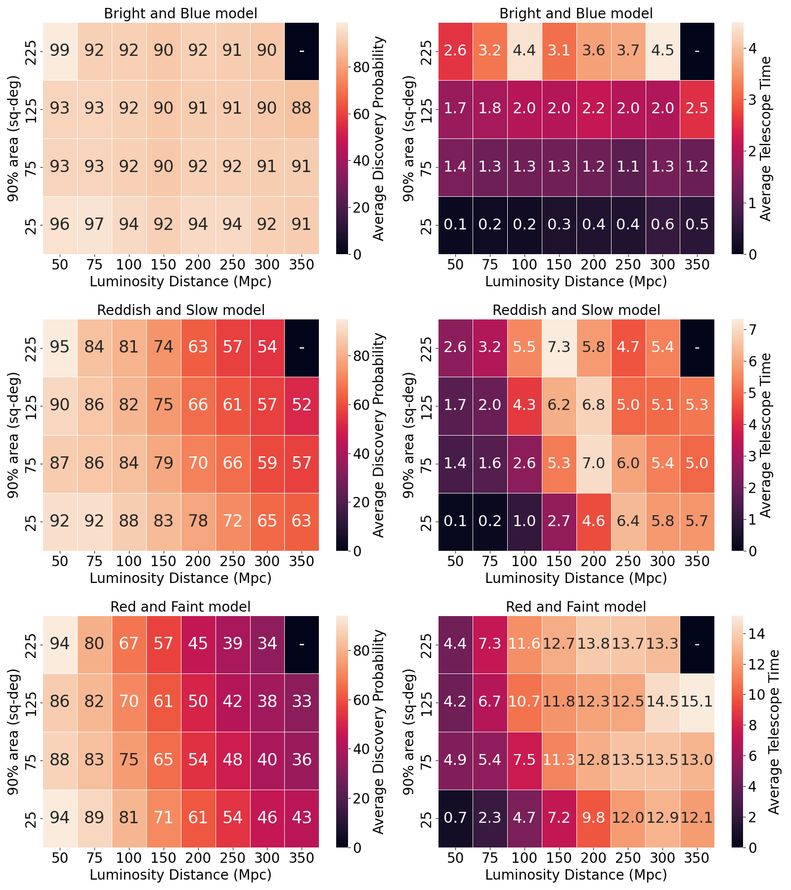
Figure 6: Using the low-TTcase Left column: Detection probability for a given luminosity distance and sky area for reddish & slow, red & faint, bright & blue in (top), (middle), and (bottom), respectively. Right column: Average required telescope time per event area as a function of luminosity distance, ordered the same as in the left column.

The plots in Figure 5 show how the low-TT strategy selects its optimized choice as compared to Top. All 4800 $P_{d,1}$ for the parameter combinations in Table 3, assuming scenario 2, for a single event simulation are shown, color coded by the required telescope time. The highest $P_{d,1}$ tend to use the highest telescope times, but there are many high $P_{d,1}$ parameter combinations $\Theta_{i}$ that use much less telescope time. The lower plot has the Top and low-TT strategies marked. Generically, our strategies prefer balanced $P_{d,1}$ and $P_{d,2}$ to maximize $P_{c}$. For the event presented in Figure 5 the low-TT configuration chosen for the first detection was core exposure $200$s($120$s) using $i$ band, the second detection was done with $300$s($200$s) in the core (outer) region, using $z$. The core (outer) region is $80\%$($90\%$) during day 1 after the burst. The Top  configuration prefers to explore the core (outer) region with $600$s ($300$s) exposures in the first detection and $300$s ($200$s) in the second detection both cases using filter z. The core (outer) area represents $70\%$($90\%$) regions. It is worth noticing that this reddish & slowmodels peaks in $i$ band around one day after the burst and in $1.2$ days in $z$ bands, however this model present a slow decaying in $z$ allowing a significant probability of discovery $2$ days after the burst.

There is the question of “when is it good enough?”, of diminishing returns. We can adopt the reddish & slow model compared to the reference strategy, for example, and work with the best $90\%$ of events. Then the low-TT at a cost of $\times 4$ more telescope time detects $20\%$ more KN and Top t the cost of $\sim 12\times$ more telescope time detects only $\sim 30\%$ more KN. Whether one is willing to accept the cost depends on the science case. For the standard siren cosmology case which wants to maximize the number of KN detected, one would prefer the maximum return of Top, but might be willing to accept the rate of low-TT. For the science case of studying the astrophysics of KN, where one wants to select good objects for detailed astrophysical study, gathering the next 10 expected in O4 might well be worth expending what Top  requires for the right events.

Returning to the performance of the strategies, we delve deeper in Figure 6 for the low-TT strategy. In this plot we present detection probability as a function of sky area. Here the distance weight in equation 3.2 becomes important. In each event, the detection probability calculated for each voxel in the skymap is weighted by the distance to that voxel to form a distance weighted detection probability for the whole event. This accurately weights the probability for the often smaller distances in the lower probability areas of the sky map (see, e.g., Singer et al. (2016a)). Thus the detection probability for bright & blue at $d_{L}=50$ Mpc can be 99% when we only cover the 90% sky probability region.

The easiest way to understand Figure 6 is to start with the right column and especially the bright & blue model. We have seen from Figure 4 that low-TT is very effective at discovery for this model and the two dimensional projection shown in Figure 6 shows little variation about that high efficiency. What variation is present is the expected loss of efficiency with increasing distance and area. In the right column for the bright & blue case, it is clear that the telescope time required increases with increasing distance and area. The increase with area is very nearly the ratio of the sky areas.

The red & faint model efficiency plot shows that the dominant variation is a decrease in efficiency with increasing distance as the faint objects fall below the limiting magnitude for the maximum exposure time. Table 3 shows a maximum exposure of 1 hour so in our 8 hour maximum night, DECam can cover 24 sq-degrees. The variation in sky area is not as dramatic as with distance and shows the success of the inner/outer split in Scenario 2, when deep exposures over the high probability area are combined with shallower exposures over the lower probability area. (Note that eq 2 was evaluated separately in each area.) The corresponding telescope time plot behaves as expected with increasing telescope time with increasing distance and area.

The intermediate reddish & slow model behaves as expected in efficiency. It is more $m_{\mathrm{lim}}$ dominated than bright & blue and doesn’t require $m_{\mathrm{lim}}$ as deep as red & faint. The smallest area bin is likely using 1 hour to maximize area coverage. The corresponding telescope time plot cell shows 5.7 hours for the average event, likely less than 8 hours because of the events with less than 24 sq-degree sky area. The telescope time plot as a whole shows a surprise. There is a peak in the time at intermediate distances and area, and then the time falls with further distance. One can see that some of the same behavior in the top row of the red & faint model telescope time plot. The explanation is that there are strategies (here meaning $\Theta_{i}$) that use high telescope time to maximize $P_{d,1}$ but these take so long to cover the area that $P_{d,2}$ is compromised by the fading of the KN, and thus $P_{c}$ is lowered. A higher $P_{c}$ is obtained by using a shorter time to cover the area to cover the area before the object fades, thus maximizing the product of $P_{d,1}\cdot P_{d,2}$.

5 Exploring Parameter Space

We have constructed 4800 parameter-set evaluations of DECam kilonova magnitudes produced by SNANA for $611$ Bayestar simulation-detected O4 binary neutron star merger events. We have developed a methodology that uses discovery and confirmation probabilities and a set of optimization rules to produce strategies optimized for the discovery of KNe under certain constraints. We have discussed maximized discovery (Top) and minimal telescope time (low-TT) already, and will discuss several more strategies in 5.2. Here we will show detailed behavior of the strategies.

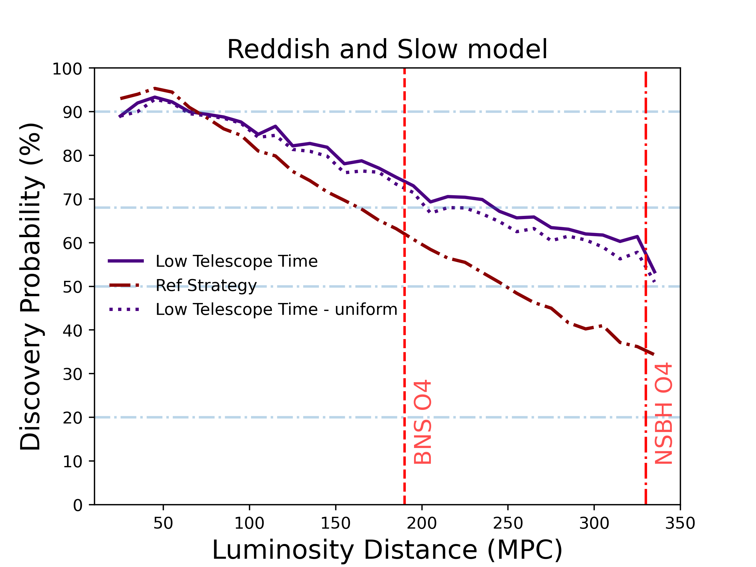
Figure 7: Upper: discovery probability vs distance for low-TT comparing Scenario 1 and Scenario 2, as well as Reference, which only uses Scenario 1. The middle and bottom plots show the exposure times that were most common when using Scenario 2, which breaks up the area into a shallower outer region and a deeper inner region of the spatial sky area.

We use the reddish & slow (GW1701817-blue, $10\times\sigma$) KN model for the results in this section unless otherwise stated. Likewise, we will use the low-TT strategy for the results in this section unless otherwise noted. To recap this strategy, we go through all combinations of inner & outer region sizes and exposure times as listed in Table 3 and present the combinations that give the lowest telescope time within $10\%$ of the highest confirmation probability strategy.

5.1 Exposure times

One of the dominant features of the observing parameters described in Table 3 is the splitting of Scenario 1 and Scenario 2. In Scenario 1, the sky is covered with uniform exposure times. In Scenario 2, we allow the splitting of the sky localization area into an outer region and a longer exposure inner region. Scenario 2 is best thought of as an homogeneous pass with a deeper exposure in the high probability region. Putting aside the distance weighting, covering a sky localization area sets a ceiling on the discovery probability to the probability contained in that area, and thereafter it is maximizing the limiting magnitude in the sky area. Our optimal selections almost always prefer Scenario 2 over Scenario 1 as implicitly or explicitly the total telescope time is constrained.

Figure 7 shows the percentage of simulations that preferred each exposure time broken into inner and outer areas. The mode of the 2-d distribution for the inner region is 20 minute exposures, with $31\%$ of events using that exposure time and $84\%$ of events using 20 minutes or less. For the outer region, the mode is 5 minutes, with $33\%$ of events using that exposure time and $74\%$ of events using 5 minutes or less. This is model dependent. The bright & blue model uses 90 seconds 99% of the time in the inner region and 60 seconds 99% of the time in the outer region. Most often, 87% of the time, this is a very small inner region of 0.3, and in 93% of the simulations chose the 0.9 outer probability area. This is the lowest exposure time combination for Scenario 2 in Table 3, and it is likely that the strategies would have used a shorter exposure time if available, although it is notable that the strategy did not prefer the available 60 sec homogeneous pass in Scenario 1. The red & faint model has a more complicated exposure time pattern for the inner area. In order of use, 2400, 600, 3600, 1200 second exposures are used in 26%, 18%, 16%, & 15% of the simulations, respectively. The outer area exposure time has a mode at 1200 seconds of 25%, with 13% and 14% for 2400 and 600 seconds respectively, and 17% of simulations use 300 seconds.

For distances out to 125 Mpc, the difference between Scenario 1 and Scenario 2 is minimal, but at around 300 Mpc using scenario 2 gains $\sim$ $5\%$-$10\%$ in discovery probability. In other words, the slope in probability vs distance is shallower for the two-zone scenario than it is for the one-zone scenario. Therefore, we believe that using the deeper in the center approach will in general be more successful the more distant the event.

Figure 8: Upper: discovery probability for the different strategies adopted in bright and dark time. Middle: heatmap showing the percentage of simulations using each filter in the first and second passes in dark time for the low-TT 10% strategy and the reddish & slow model. Lower: heatmap showing the percentage of simulations using each filter in the first and second passes in bright time for the low-TT 10% strategy and the reddish & slow model.

5.2 Filter Choice and bright/dark nights

In following-up an LVK event, there is a similar chance of observing in dark conditions as in bright conditions. In Figure 8 we show the effect of dark versus bright time. The bright/dark distinction is handled in our methodology via a change in $t_{\mathrm{eff}}$ as seen in Table 1. Bright time lowers discovery probability by $5-10\%$, with the loss being mitigated by filter choice and exposure times. The filters used in the two passes are,in dark time, $rr(33\%),zz(50\%),ii+iz(17\%)$. In bright time the filters are $zz(71\%),ii+iz(25\%)$. The filter choices are strategy dependent, and, for comparison, the Top strategy used in dark time $rr(12\%),ri(7\%),rz(27\%),iz(29\%)$, and $zz(17\%)$ and in bright time $iz(45\%)$ and $zz(41\%)$. The filter choices are also model dependent, driven by the color evolution of the reddish & slow model as seen in Figure 3. The $g$ filter is never going to be favored in this model, $i$ will be picked the first night, $z$ on the second, except that it is easier to go deeper in $r$ than in $i$. We can predict that the filter selection for red & faint model will be nearly the same but that the bright & blue model would predominately use $g,r$. Notably, it is not straightforward for us to say which filters we use in our best strategy.

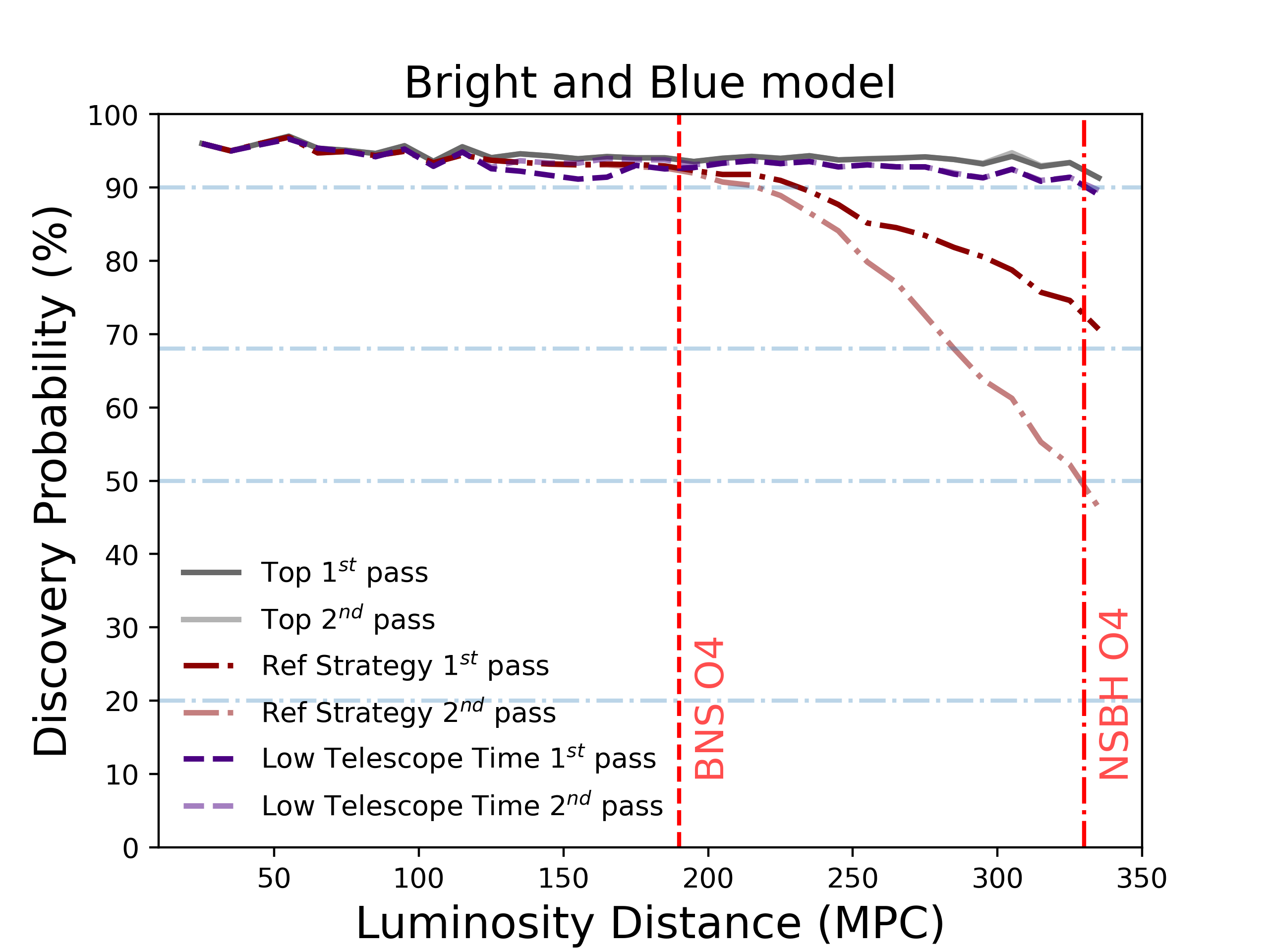
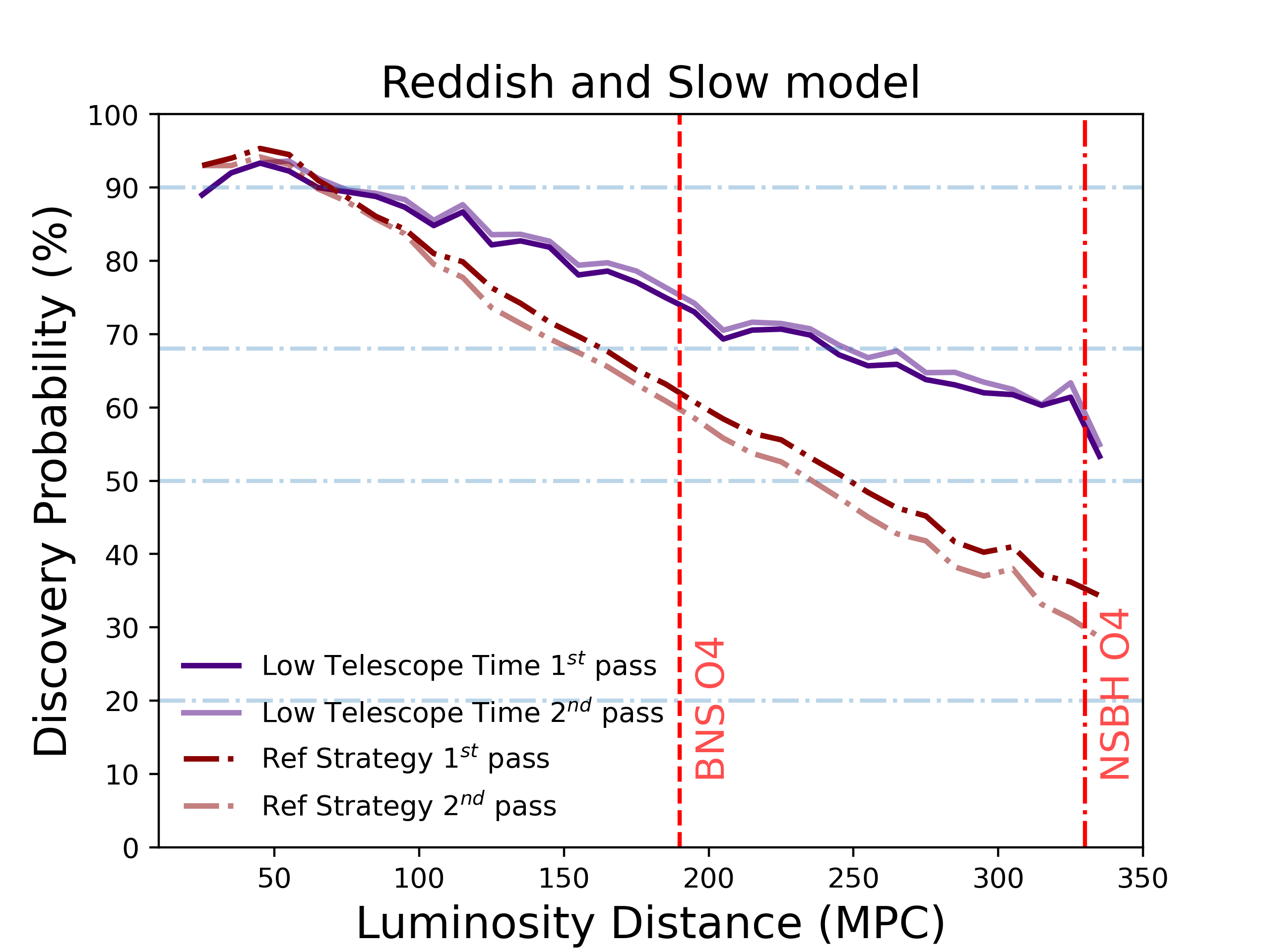
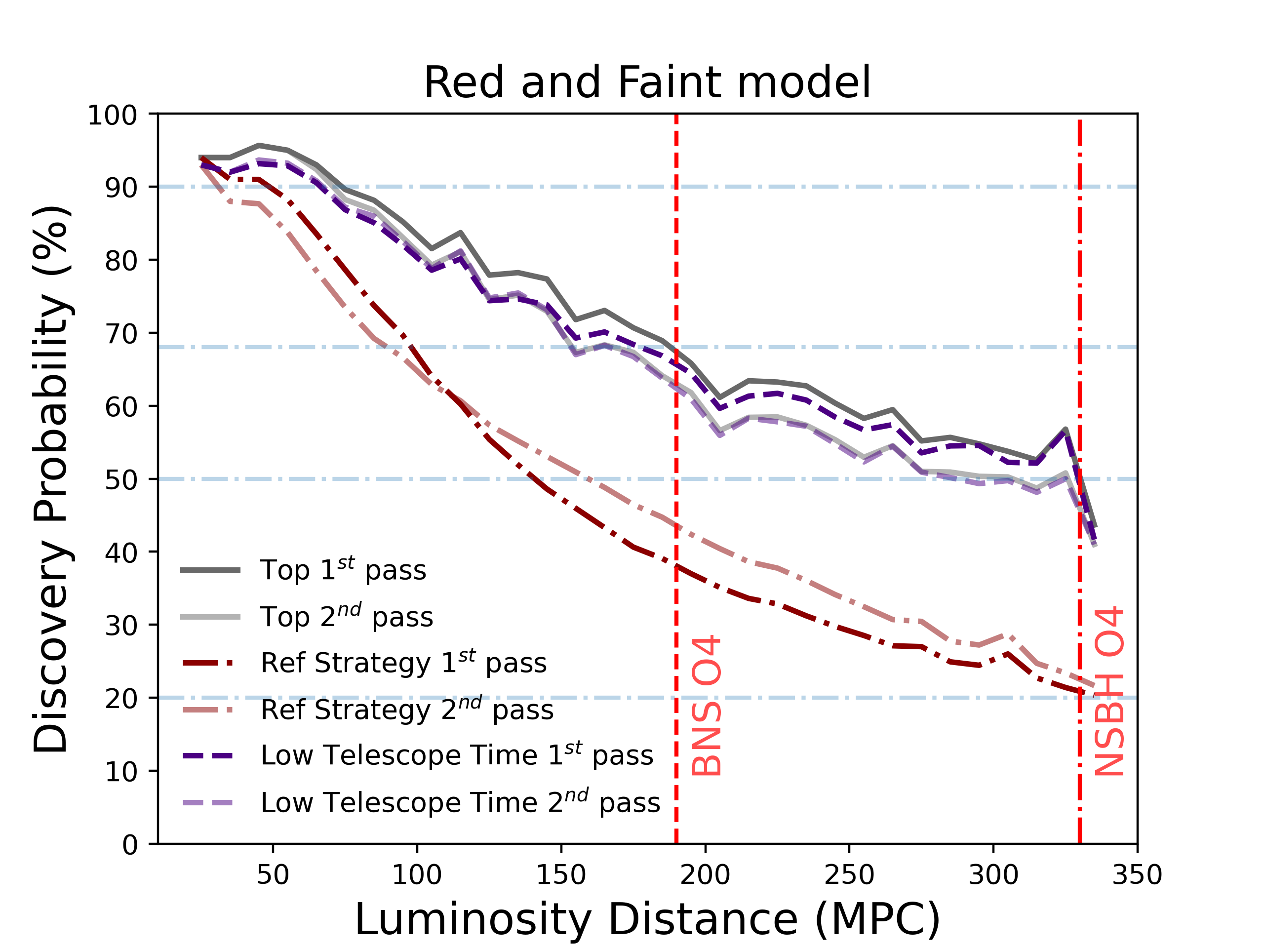
Figure 9: Discovery probability vs distance to event for the low-TT observing strategy in the first and second passes compared to the reference strategy for KNe described by model bright & blue (upper), with wide priors reddish & slow  (middle), and red & faint (bottom).

5.3 Impact of the two-detection requirement

Detecting a counterpart twice in DECam images is an important step in our experience, as it allows one to distinguish extragalactic transients from asteroids or other objects within a short period of time. This requirement is common, for example Zhu et al. (2021), Sagués Carracedo et al. (2021), and Petrov et al. (2022) all demand two detections for a confirmation of a kilonova transient. Also important is covering the sky area with multiple filters to distinguish the KN from other transients.

The DECam search does not happen in isolation, and we do emphasize the importance of the broader GW community during these times. While our programs’ main line is to proceed to confirmation via a second image, smaller telescopes may chose to follow-up first image preliminary candidates in order to efficiently reduce the candidate list that will be sent to expensive spectroscopic efforts. There are reasons to be interested in both $P_{d}$ and $P_{c}$.

In Figure 9, we show $P(\mathrm{discovery})$ in the first detection, $P_{d,1}$, compared to the second detection, $P_{d,2}$. In the low-TT strategy the detection probability remains nearly constant between pass 1 and pass 2. This is not the case for the reference strategy. For the reddish & slow model there is a nearly constant offset between $P_{d,1}$ and $P_{d,2}$ favoring within a few percent the second pass. It is worth noticing that this is our model that peaks at later times, and therefore the second pass might happen closest to the peak. However, the difference is inside the $68\%$ confidence interval as presented in Figure 4. For the red & faint model the $P_{d,1}$ is higher at $d<100$ Mpc, and $P_{d,2}$ is higher at $d>100$ Mpc. For the bright & blue model, we see the reference strategy become less efficient than the low-TT strategy at $d>220$ Mpc, as both $P_{d,1}$ and $P_{d,2}$ drop with increasing distance. We infer that the low-TT strategy strongly prefers to balance $P_{d,1}$ and $P_{d,2}$.

5.4 Other Strategy options

Our choice of optimization has flexibility. We might place a high priority on the earliest possible discovery, or we may have lost several nights due to weather conditions and need to find an optimal approach for the first clear night several days after trigger. Let us, therefore, explore three other optimizations:

1. Early Discovery (ED) is the $\Theta_{i}$ that produces the earliest confirmation limited by the $P_{c}$ from low-TT($5\%$) for each $S_{i}$.

2. Late Discovery (LD) is the $\Theta_{i}$ that produces the latest confirmation limited by the $P_{c}$ from low-TT($5\%$) for each $S_{i}$. This family is intended to find a competitive strategy when one cannot observe during some early/intermediate nights or in case the event was not confirmed in the first days.

3. Half Nights (HN). This family is intended to find a competitive strategy when one cannot observe half the night- if the object rises or sets for example, or the telescope is only allocated for half nights. Thus, from the subset limited by the $P_{c}$ from low-TT($5\%$) for each $S_{i}$ configurations we constrained the strategy to have both passes in less than $4$ hours if they are in the same night or each of the passes takes $4$ hours individually if they are in different nights. In this exercise we consider the observation starts in the first half of the night.

All those configurations are restricted in telescope time. In Figure 10 we show the distributions of the time of second pass completion relative to the merger. It is in the second pass that we achieve a confirmation. The ED scenario not surprisingly has earlier times than Top, and, by design, earlier times than LD. The late discovery strategy has a different optimization and thus a different use. If the first night or two are not useful for observations, then the LD strategy is useful for pursing the discovery at late times. It peaks around $2.5$ days after the merger. Note that this strategy is optimized on $P_{c}$, so does not describe the case where the event is unobservable due to clouds for a night or two, but rather is working the scenario where the object is detected but cannot be confirmed for several days. Figure 10 suggests that since $P_{d}$ is on the first night, the most likely night to capture the confirmation pass is the third night. LD is representative of the kinds of strategies that would be necessary to deal with weather. The Half Night strategy enforces a limitation to the amount of time spent in pass 1, and the resulting performance is similar to low-TT in terms of both $P_{c}$ and telescope time expenditures, although without the guarantee of being within $10\%$ of the best strategy, Top.

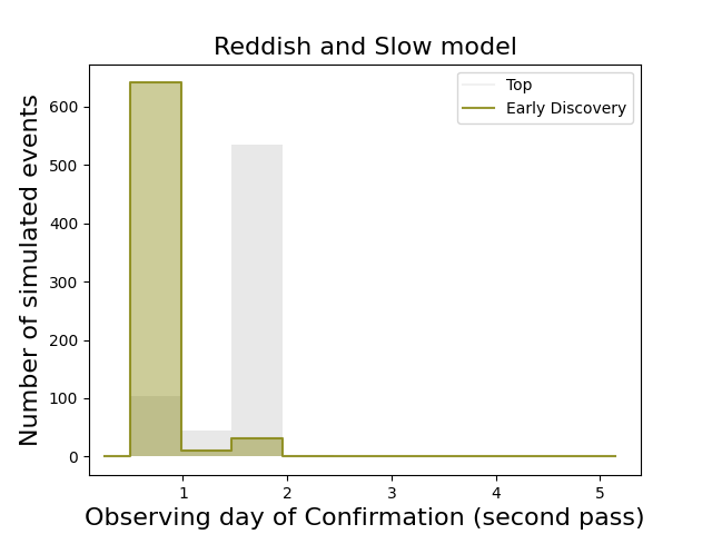
Figure 10: Distribution of confirmation day using the reddish & slow model. The upper panel depicts the time of confirmation probability (i.e. how many days it took to observe the area twice) for our ED strategy and the bottom panel depicts the LD strategy. Most simulated events are confirmed by the first day. For reference we also show the distribution using the Top strategy, which has no restrictions on when to perform the follow up.

Figure 11: We illustrate the flexibility of the strategy families. We present the curves constrained with $5\%$ of Top strategy, e.g. low-TT ($5\%$) and derived strategies. Upper: reddish & slow. Lower: red & faint. Half Nights are not always available. For reddish & slow 395 half nights strategies produced detections, while for red & faint 137 half nights strategies produced detections. As the exposure times skew deep, the success rate is likely anti-correlated with sky area.

Figure 11 shows the discovery probability versus distance for the strategies discussed here. For the reddish & slow model, all of our strategies have roughly equally performance (but see the Top outperforming low-TT by the amount it is allowed to) although with different telescope time cost. This is true to $d=180$ Mpc, but after that, the LD strategy becomes less efficient. For the red & faint model, we see, interestingly, that the low-TT and Top strategies have equal performance. Finally, the Half Night strategy performs very well until $d=180$ Mpc, then becomes infeasible.

For the reddish & slow model, the ED strategy for exposure time distribution is more or less equally split among the possible outer/inner exposure time pairs in Table 3 up to the outer region exposure time of 600 secs, with the most likely outer exposure time of 300 seconds. There are no outer exposure time greater than 600 seconds nor inner exposure times greater than 2400 seconds. The LD strategy’s most likely exposure time is 1200 seconds, and the strategy tries to cover the largest inner region possible. The outer region has the most likely exposure time of 300 seconds and is never longer than 600 seconds. The strategy is to cover the largest inner region possible with relatively shallow outer region exposures. The second pass exposure time is weighted deeper than the first pass but the most likely exposure time remains 1200 seconds. The Half Night strategy for exposure time distribution is 31% of simulations using 1200 seconds, and 17% using 2400, most often in an 0.7 inner core region. The outer region uses 300 and 600 second exposures over half the time.

For the red & faint model, the ED strategy for exposure time distribution is deeper than for the same in reddish & slow, preferring 600, 1200, 2400 seconds instead of 600 and 1200, never using 90 second exposure times for the inner core like 15% of the reddish & slow simulations do. The LD strategy simulations 57% of the time use 600, 1200, or 2400 second exposures but uses a wide range of inner areas. The outer region uses all exposure times from 60 to 2400 seconds but is most heavily weighted towards 300, 600, and especially 1200 seconds. The Half Night strategy exposure time distribution is complicated, using a wide variety of inner areas and exposure times skewing deep at 1200 and 2400 second exposures. The outer region is similar, although here, as most often throughout the strategies, the outer region coverage of 0.9 is preferred.

Table 6: Average telescope time per event in hours required for two detections, discovery and confirmation, as in Table 5.

Strategy	Telescope time (hours)
bright & blue	$50\%$	$90\%$	$100\%$
Early Discovery	0.4	1.0	1.4
Late Discovery⋆	0.4	1.0	1.4
Half Nights⋆	0.4	1.0	1.3
Low TT - Bright Night	0.5	1.2	1.6
reddish & slow
Early Discovery	3.3	4.3	4.4
Late Discovery⋆	3.1	3.9	4.0
Half Nights⋆	2.9	4.0	4.0
Low TT - Bright Night	3.2	4.7	5.3
red & faint
Early Discovery	6.7	7.7	7.8
Late Discovery⋆	6.6	9.1	9.1
Half Nights⋆	2.6	3.9	4.0
Low TT - Bright Night	7.6	9.6	9.9

Strategy	Detection Prob.	Filter	Exposure Time	Integrated Prob. Area	Total Telescope time	Confirmation Day
	(%)		outer, inner (sec)	outer, inner	($2$ detections, hours)	(days after alert)
Top	75	r	3600, 5400	0.9, 0.5	14.7	1.5
LTT	68	z	300, 1200	0.9, 0.7	3.2	1.0
HN	69	z	600, 1200	0.9, 0.7	3.5	1.0
ED	65	i	600, 1200	0.9, 0.8	2.9	0.5
LD	65	i	600, 1200	0.9, 0.7	3.5	2.0
Ref	48	i	90	0.9	0.5	1.5

Table 7: Excerpt of output csv for example simulated event. Table displays the highest probability configuration for each strategy using scenario 2 (using deeper exposures in higher probability sky area) for the bright & bluemodel. Exposure time outer, inner represent the time used for the shallow and deep area used out to the area listed in column Integrated Prob. Area outer, inner. This summary information will be used in the decision tree of which strategy to use for an actualy LVC event trigger. Dual exposure times and probability areas describe the exposure time and area covered for the ’deep’ inner and ’shallow’ outer region exposures of Table 3.

6 Real observations

We have presented a variety of strategies optimized for a variety of purposes. Here we describe how to use them when an observing team receives a LVK alert.

We can compute $P(\mathrm{confirmed})$ for the grid of $\Theta$ in Table 3 (both scenarios) using estimations of $t_{\mathrm{eff}}$  for the upcoming night. Given the $\Theta_{i}$, we can choose a strategy to follow, placing the Top, low-TT, ED, or Half Night optimizations on as appropriate for the event. The optimization gives us the single $\Theta_{i}$ for each of the strategy families.

The strategy computation takes about 30 minutes on a single core. This includes the four strategy families (Top, low-TT, ED, Half Night), as well as considerations about bright/dark time. The time to complete the computation can be brought down to $<1$ second by using the simulations as an approximation for the real event. Here our approach would be to choose a $\Theta_{i}$ by nearest neighbor search or to build a simple neural net on the simulation parameters and $P(\mathrm{confirmed})$ to chose $\Theta_{i}$.

The choice of the KN model is important. For example, if we are very early on-sky, with great observational conditions for just a couple of hours, or some limitation in telescope access is imposed upon us, we might also consider a fast detection of a blue flash (bright & blue model). This strategy could be interesting in particular for low-TT due to the cost of deep exposures over a wide area.

There is also a flow of decision making external to what we have described. Whether or not the there is a short GRB, we choose distinct approaches. In the case that there is, we are likely looking for a GW170817-like event (bright & blue). If not, then a conservative model is indicated (reddish & slow), as we might not be looking for an event with a high inclination angle. If the alert indicates it is a NSBH merger, then the KN is likely more consistent with the red & faint model. After this if there is a possible half night strategy, they are low budget and high performing by definition. It also gives time for us to use spectroscopy to confirm quickly. In an observing run where we expect 1 BNS merger every month, we could plan on allocating telescope time through the run considering the amount of telescope time remaining versus where the particular event lies in a SNR distribution Chen & Holz (2014) or among a population of simulated events. This would lead to spending more toward the end of the run if considerable time was left, or spending more if it was a particularly good event compared to the simulations.

6.1 Plan for Usage

To demonstrate how using this code might work during a real GW follow up campaign, we randomly select one of the simulations used in this analysis. For this exercise, we are assuming the LVK trigger announcement was received towards the beginning of the night, meaning we will aim to be on sky within a few hours of merger. The general logic flow for determining the observing plan goes as follows:

1. Assess our external factors:

   1. How many hours are we allotted for the night and telescope availability,

   2. Sky conditions,

   3. Check if there was a GRB reported in the area at the same time (as was the case with GW170817). This last criterion is important for choosing a KN model to use.

2. Using the external factors as input, run the code.

3. Assess output csv, see Table 7. Here we would decided if this is an event that we would like to follow-up, considering the discovery probability.

4. Choose filters, exposure times, and area coverage from strategy and compile observing plan.

While most external factors are easy to identify, choosing which KN model to follow may not be obvious and will depend on the particular science goal of the project. For instance, if one’s science goal is to have the most complete set of KN, then using the faintest KN model is useful and thus red & faint is the favored model. For simplicity, in this example we will assume a GRB was reported within the LVK sky area, thus favoring bright & blue. Once the code has generated an output csv file, we can compare strategies.

The configuration with the highest detection probability for each strategy is displayed in Table 7. Here we can see for this event the Top yields the highest probability of detection, as expected. In this example, however, the Top strategy more has a factor of almost $\sim 5$ in the amount of telescope time needed for any other strategy for only $\sim 7\%$ more probability of detection.

7 Discussion

In this paper our science goal is to maximize the number of KN with GW measured $d_{L}$ and securely identified redshifts. We put high weight on completeness of detection of the KN, given the considerable uncertainty in the KN population. Our strategies go deep. The strategy chosen by our optimization in low-TT mode and reddish & slow kilonova reach $m_{\mathrm{lim}}(10\sigma)$ of $r\geq 24.4$ and $z\geq 22.9$ for the $\geq 1200$ second exposures (see Table 2) for the inner regions of $47\%$ (as defined in Table3) from our set of $611$ simulations, regardless of distance (see Figure 7).

We can gain insight into our results by comparing how the literature handles a set of 3 questions:

1. the modeling of GW merger event distance and sky area distribution,

2. the range of KN model physical parameters, including inclination angle

3. the telescope, search and cadence, detectability versus distance and $m_{\mathrm{lim}}$.

The GW event properties: We simulate a merging NS-NS population expected in O4 given the expected LIGO sensitivities, drawing from the NS population, simulating the GW waveform and projecting onto a GW observatory network, and converting the GW observations to skymaps. Our draw, simulate, project, and form skymaps approach has been performed before (Petrov et al. (2022); Chen et al. (2021)), though it sometimes is done without skymaps (Zhu et al., 2021). There are simplified approaches. One can just assume a KN population to observe (Sagués Carracedo et al., 2021; Setzer et al., 2022; Chase et al., 2022). Or one can use toy GW models, such as a low-significance event skymap at 200 Mpc (Coughlin et al., 2020). All of these approaches assume the KN properties are independent of the GW event properties, other than distance. Colombo et al. (2022) performs the more sophisticated analysis of connecting the KN properties to the GW event properties by going through the chirp mass and mass ratio, which informs $M_{\mathrm{ej}}$ and $v_{\mathrm{ej}}$. Of the analyses that go through the draw, simulate, and project methodology, all assume the SN $>8$ or network SN$>12$ in selection except for Petrov et al. (2022) which derive the effective SN threshold from the published GWTC events. They find that there will likely be more events with $90\%$ credible sky areas $>300$ sq-degrees than we simulate, but do not include in our followup identification analysis. For the analyses that extend to jet production (e.g., Zhu et al. (2021); Colombo et al. (2022)) about $10\%$ of events are sufficiently pole on to for jets to be observed. It is worth noticing, however, that the simulations used are based on the assumptions about the sensitivity of the LVK detectors. The predicted sensitivities are roughly equivalent to those anticipated around mid-2022 for the upcoming observing cycle O4. The actual operational conditions diverge from these expected design sensitivity. The Virgo detector, for instance, has not joined in the O4 from its beginning, and it remains uncertain whether it will achieve the proposed sensitivity for this cycle.

Moreover, the KAGRA detector has participated in the run for a limited period, but at a reduced binary neutron star (BNS) inspiral range than that estimated here (80 Mpc). The adjustments in observational capabilities were publicly disclosed only when this work was nearing completion. As a result, the predictions offered in this study may be optimistic when evaluated in the context of the present O4 run. Nonetheless, these forecasts retain their significance, in terms of methodology for guiding observations, even if they do not reflect the current O4 schedule.

Kilonova physical properties and inclination angles: We have only one well studied KN in the literature, so there is considerable uncertainty in the KN population. The literature has three ways of modeling KN- using model atmospheres as building blocks (e.g. Kasen et al., 2017)), full physical models of KN atmospheres (e.g. Bulla, 2019; Wollaeger et al., 2021)), and using scaling relations and fitting functions from relativisitc numerical simulations (e.g., Dietrich & Ujevic (2017); Coughlin et al. (2019)). The first two approaches are parameterized by at least three variables (for us, $M_{\mathrm{ej}},v_{\mathrm{ej}},\log{X_{\mathrm{lan}}}$). The Bulla models, which include inclination angle explicitly, are widely used in the relevant literature (e.g., Coughlin et al. (2020); Sagués Carracedo et al. (2021); Zhu et al. (2021); Petrov et al. (2022)). Often, analyses in the literature will set up a grid of KN parameters and inclination angles and proceed to simulate detection of each entry in the grid, either for a fixed distance of for NS merger population. Typically the fraction of models detected is termed the detection efficiency. This makes the detection efficiency depend on the model space in unfortunate ways. Consider the case of inclination angle dependent KN properties. One can set up a grid of inclination angles. Better would be to use the probability distribution function of inclination angles for an random isotropic inclination sample, $PDF(i)\propto\sin(i)$. This weights edge on, i.e. red and faint, KN more than a grid is likely to. The inclination angles sample selected by a GW detector network search isn’t isotropic. The amplitude of the strain detected is generically described by $PDF(i)=0.076076(1+6\,cos^{2}(i)+cos^{4}(i))^{3/2}\sin(i)$, that it, GW observatories prefer inclination angles near $30^{\circ}$ (Schutz, 2011). For the Bulla models, this could be accounted for by using Bayesian priors on the models. It would be interesting to have a version of the Setzer et al. (2022) KN population absolute magnitude distribution weighted by the expected GW network inclination angle distribution. In our work, we use Bayesian model averaging on our calculated detection probabilities. We do not model polar vs equatorial directly, but one could map the appropriate blue and red Bayesian model average into those. Our red & faint average absolute magnitude is about 0.4 mags fainter than the brighter peak of Setzer et al. (2022).

Detection efficiency: Our study is for DECam on the Blanco 4m with its 3 sq-degree field of view, covering the $90\%$ credible sky area using real cadences in 2 passes to ensure a confirmation. A complete search and discovery simulation over full LVK simulated skymaps has been done by Coughlin et al. (2020) and Petrov et al. (2022). As the 1m class telescopes have very large fields of view, up to the ZTF 47 sq-degrees, much more common in the literature is to assume a KN model, usually a GW170817 analog, and ask what exposure time or limiting magnitude is necessary to detect it. If instead of Bayesian model averaging of the detection probability we had used Bayesian model average absolute magnitudes, our study would be very different. The average absolute magnitudes for our bright & blue, reddish & slow, and red & faint models for $r$-band are $-16.3,-15.2,-14.2$ respectively. In 100 seconds, DECam reaches $r=23.0$, sufficient to detect $M_{r}=-15.2$ to 500 Mpc. In 1200 seconds, DECam reaches $r=24.4$, sufficient to detect $M_{r}=-14.2$ to 500 Mpc, and GW170817’s $M_{r}=-15.5$ to 1 Gpc. Why then do events at $d_{L}=200$ Mpc, have in our study detection probabilities $P_{d}$ of 90%, 73%, & 60% for the bright & blue, reddish & slow, and red & faint models, respectively, using the low-TT strategy, and routinely require 60-90 second exposures for bright & blueand 300-1200 second exposures for the last two models. The effect of using eq 2 is to extend the search to lower $M\_\mathrm{ej}$ and $\log{X_{\mathrm{lan}}}$ and thus lower luminosities. Our method of accounting for uncertainty in the KN population is driving our results. If we adopt the Coughlin et al. (2018) model parameters and uncertainties, our detection efficiencies would increase and exposure times decrease. Using the GW170817 absolute magnitude for detection is likely over-optimistic, as suggested by Colombo et al. (2022) placing GW170817 at the $75^{th}$ percentile bright, and Setzer et al. (2022) placing it at $95^{th}$ percentile bright. The studies using 1m class telescopes are most likely to assume GW170817 analogs, though Petrov et al. (2022) uses both that and a lower luminosity, red model, and Sagués Carracedo et al. (2021) does a careful analysis of viewing angle dependent models. The studies assuming the Rubin Observatory (Cowperthwaite et al., 2019; Chen et al., 2021), or a variety/network of telescopes (Coughlin et al., 2020; Chase et al., 2022) tend to analyze detection probabilities for lower luminosity events. In summary, one will have to be careful comparing our detection probabilities with others in the literature, which often use a single luminous model or evaluate and average detection efficiencies over a grid of models using a uniform prior. In our language, “chance of finding it” in Fig 4 is to be interpreted as “fraction of models detected given our priors on the space of models”.

Table 8: LVC GWTC events (O1-O3) containing neutron stars and with $M_{2}<5M\odot$ and SNR$>8$.

id	$M_{1}$	$M_{2}$	distance	SNR	class
	($M_{\odot}$)	($M_{\odot}$)	(Mpc)
GW170817	1.5	1.3	40	33	BNS
GW190425	2.0	1.4	160	13	BNS
–
GW190814	23.2	2.6	240	22	BH-NS
GW200105_162426∗	9.0	1.9	270	14	BH-NS
GW200115_042309	5.9	1.4	290	11	BH-NS
GW190426_152155	5.7	1.5	370	10	BH-NS
GW191219_163120	31.1	1.2	550	9	BH-NS
GW190917_114630	9.3	2.1	720	10	BH-NS
GW200210_092254	24.1	2.8	940	8	BH-NS

Note. — $\Delta m_{\mathrm{lim}}(10\sigma-5\sigma)=0.75$ mags.

Note. — Table of means, $\mu$, and standard deviations, $\sigma$, of the Gaussian priors on the Kasen models parameter ranges. The Kasen models have parameter ranges of:

0.001 M_$\odot$ $\leqslant$ $M_{\mathrm{ej}}$ $\leqslant$ 0.1 M_$\odot$

$-9\leqslant\log({X}_{\mathrm{lan}})\leqslant-1$

$0.03c\leqslant v_{\mathrm{ej}}\leqslant 0.3c$

Note. — ^⋆ Due to the strong constraints in Half Night and Late Discovery, they are not always available for a given GW event simulation. For bright & blue, reddish & slow, and red & faintmodels, these strategies are only defined for 602, 496, and 131 simulations respectively in the half night scenario. While Late discovery is defined for 532, 511, and 251

Note. — SNR is the matched filter SNR. GW200105_162426^∗ has $p_{\mathrm{astro}}=0.3$ is thus considered a marginal candidate. Only 2 events have a 90% confidence sky area of $<30$ sq-deg, 2 at $<300$ sq-deg, and 3 at $<400$ sq-deg. The median sky area is 1700 sq-deg. Data from https://www.gw-openscience.org/eventapi/html/allevents/

7.1 Applicability to NSBH and mass gap events

For standard siren studies, NSBH mergers are just as valuable as BNS mergers, as long as they produce electromagnetic counterparts. NSBH merger events have higher distances for similar SNR than BNS mergers, as can be seen in Table 8,

The dominant factor for their use in standard siren cosmology is the probability of a KN given a NS-BH merger. No counterpart to a NSBH merger has been detected (e.g. Morgan et al. (2020); Anand et al. (2020); Kawaguchi et al. (2020a)). Zhu et al. (2021) argue that no detectable KN counterpart was expected for NSBH mergers in O3. Kawaguchi et al. (2020b) and Darbha et al. (2021) study the brightness of KN from NSBH mergers, and Drozda et al. (2020) does the same for mass-gap objects. The summary is that only a fraction of NSBH events will produce KN, primarily those mergers with low mass ratios and high spin.

The Kawaguchi et al. (2020b) models have absolute magnitudes that peak for $r,i$ at $-14.5$, $-15.0$ respectively. There is a spread of about 1 magnitude fainter in the i-band absolute magnitude, going fainter as the binary mass ratio increases and the effective spin gets smaller. Our red & faint model has an $i$-band absolute magnitude of $-14.5$, midway through the range of Kawaguchi et al. (2020b). Petrov et al. (2022) adopt the Bulla (2019) models, broken into BNS and NSBH models both optimistic ($M_{\mathrm{ej}}=0.05,0.08$) and conservative ($M_{\mathrm{ej}}=0.01,0.01$). The optimistic BNS model has an absolute magnitude in the r-band of -16.0, the conservative NSBH model of -14.8; these correspond well to our bright & blue and red & faint models, respectively. Taking our red & faint model as appropriate for dynamical ejecta dominated NSBH mergers, our low-TT strategy has $50\%$ detection probability out to 330 Mpc (see Figure 4). Our strategies are sufficient to obtain the majority of NSBH events that have EM counterparts if they are at distances $\leq 330$ Mpc.

7.2 Blanco/DECam and Rubin LSST

It is of interest to compare the strategies defined here with the program outlined in Chen et al. (2021). They assume inclination independence and a GW170817-like KN, and argue for two filter observations. The program conservatively assumes $30\%$ of A+ events by dedicating 7 hours of Rubin Observatory time in 30s exposures, capturing 12/year. Our expectation is that the Rubin ToO program will use 3% of the available LSST time, so on order of 100 hours which can pursue all BNS events in LVK O4 assuming 1/month and 8 hours per event, so pursuing light curves. Alternatively and more likely, Rubin will choose to observe the 50% best events by sky area in both the BNS and the NSBH categories. In this scenario a good use of DECam/Blanco would be to follow-up the others that have sky area $<300$ sq-degrees. Table 5 suggests this would be viable.

In fact, if the results of Petrov et al. (2022) hold, then there will be many merger events containing NS that have sky areas greater than 300 sq-degrees; our simulations would have to be extended by another $\sim 360$ events all with sky area $>300$ sq-degrees to match their statistics. For the bright siren cosmology every NS event is important. We demonstrate here that the Blanco/DECam especially in combination with the Zwicky observatory and its counterparts PS1, OAJ, LS4, are capable of following up the sources with sky area $<300$ sq-degrees. The optimal use of the Vera C. Rubin Observatory, with its immense etendue, is to followup the LVK sources with $>300$ sq-degrees. The combination of sky coverage and depth is unmatched. Petrov et al. (2022) predicts the median sky coverage for BNS events in O4 is $1820^{+190}_{-170}$ sq-degrees and the median luminosity distance is $352\pm 10$ sq-degrees, and the NSBH median distance further away. For the Rubin FoV of 9.6 sq-degrees, the number of exposures to cover the sky area once is $\approx 200$, which at 100 second exposures can be done in less than 6 hours, assuming a reddish & slow model and 1.2 mags deeper $m_{0}$ for Eq. 1. Likely one could build a two-visit strategy that would take 10 hours per event, allowing Rubin to followup 10 additional events per year without light curves. The Rubin time-domain ecosystem of data, brokers, and routine spectroscopic follow-up is likely to minimize positives, though perhaps not until after O4.

As discussed in Morgan et al. (2020); Garcia et al. (2020); Tucker et al. (2022), the need for coordination with spectroscopic telescopes is vital in identifying the true counterpart. Given there has only been one confirmed optical counterpart, there is uncertainty in the expected light curve from photometric data.

8 Conclusion

In this paper, we create families of observing strategies that optimize the probability of detecting a KN within DECam’s images. We examine various filter choices, depths, area coverage, and cadence of observations in order to ensure optimal chance of detection. Given the expanded range of sensitivity in future LVK observing runs, deeper exposures will be necessary in order to be sensitive to the quickly fading counterpart. As we do not have unlimited time for such follow ups, we examine how we can optimize our chance of detection while taking into account real world constraints.

We chose to optimize our strategies based on the probability of detecting the KN within two images that are at least 30 min apart. This constraint is put in place in order to help eliminate asteroids and other sources of noise. We explore two different types of observing scenarios. The first is a homogeneous covering of the sky area with a single exposure time, and the second uses deeper exposures in the higher probability sky areas and shallower exposures on the rest of the area. We then categorize our strategies by observational constraint, where each family of strategies is taken from the top $10\%$ or $5\%$ of Top strategies. The Top strategies use all available resources, and are useful as a benchmark for the full detection capability of the DECam.

Examining each of the realistic observing scenarios, we find we can achieve $\sim 75\%$ to $80\%$ probability of detection out to $190$ Mpc (the nominal limit of LVK BNS range) for a wide rage of KN parameters (reddish & slow), $\sim 65\%$ for a fainter and redder KN (red & faint) and over $90\%$ for a bright & blue model along the full range of distances limited to $330$Mpc. Additionally, we provide the mean detection probability and total telescope time required for detection and confirmation in each KN model for a given range of GW event area and distance in figure 6. In particular, this plot might be used as a guide on how likely it is to succeed in KN detection of specific future events considering a trade-off between time budget and optimal chances.

While DECam will continue to be the optimal camera in the southern hemisphere during the next observing run, the efforts to detect the next KN optical counterpart will be greatly aided by other telescopes that are planned to be online during this time. For example, the expected addition of the Simonyi Telescope at the Vera Rubin Observatory.

References

- Abbott et al. (2017) Abbott, B. P., Abbott, R., Abbott, T. D., et al. 2017, ApJ, 848, L13, arXiv:1710.05834
- Abbott et al. (2017a) Abbott, B. P., Abbott, R., Abbott, T. D., et al. 2017a, The Astrophysical Journal, 848, L12
- Abbott et al. (2017b) Abbott, B. P., Abbott, R., Abbott, T., et al. 2017b, Astrophys. J. Lett, 848, L12
- Abbott et al. (2018) Abbott, B. P., Abbott, R., Abbott, T., et al. 2018, Living Reviews in Relativity, 21, 3
- Abbott et al. (2020) Abbott, B. P., Abbott, R., Abbott, T. D., et al. 2020, Living Reviews in Relativity, 23
- Abbott et al. (2021) Abbott, R., Abbott, T. D., Abraham, S., et al. 2021, ApJ, 915, L5, arXiv:2106.15163
- Abbott et al. (2021) Abbott, R. et al. 2021, Phys. Rev. X, arXiv:2111.03634
- Abdalla et al. (2022) Abdalla, E., Abellán, G. F., Aboubrahim, A., et al. 2022, Journal of High Energy Astrophysics, 34, 49
- Anand et al. (2020) Anand, S., Coughlin, M. W., Kasliwal, M. M., et al. 2020, Nature Astronomy, 5, 46
- Anand et al. (2021) Anand, S., Coughlin, M. W., Kasliwal, M. M., et al. 2021, Nature Astronomy, 5, 46
- Andreoni et al. (2017) Andreoni, I., Ackley, K., Cooke, J., et al. 2017, PASA, 34, e069, arXiv:1710.05846
- Andreoni et al. (2019) Andreoni, I., Goldstein, D. A., Anand, S., et al. 2019, ApJ, 881, arXiv:1906.00806
- Andreoni et al. (2019) Andreoni, I., Goldstein, D. A., Kasliwal, M. M., et al. 2019, arXiv preprint arXiv:1910.13409
- Arcavi et al. (2017) Arcavi, I., Hosseinzadeh, G., Howell, D. A., et al. 2017, Nature, 551, 64, arXiv:1710.05843
- Ashton et al. (2020) Ashton, G., Ackley, K., Magaña Hernandez, I., & Piotrzkowski, B. 2020, arXiv e-prints, arXiv:2009.12346, arXiv:2009.12346
- Balasubramanian et al. (2021) Balasubramanian, A., Corsi, A., Mooley, K. P., et al. 2021, ApJ, 914, L20, arXiv:2103.04821
- Bom & Palmese (2023) Bom, C. R. & Palmese, A. 2023, arXiv e-prints, arXiv:2307.01330, arXiv:2307.01330
- Bulla (2019) Bulla, M. 2019, MNRAS, 489, 5037, arXiv:1906.04205
- Buonanno et al. (2009) Buonanno, A., Iyer, B. R., Ochsner, E., Pan, Y., & Sathyaprakash, B. S. 2009, Physical Review D, 80
- Chase et al. (2022) Chase, E. A., O’Connor, B., Fryer, C. L., et al. 2022, ApJ, 927, 163, arXiv:2105.12268
- Chen et al. (2021) Chen, H.-Y., Cowperthwaite, P. S., Metzger, B. D., & Berger, E. 2021, ApJ, 908, L4, arXiv:2011.01211
- Chen et al. (2018) Chen, H.-Y., Fishbach, M., & Holz, D. E. 2018, Nature, 562, 545
- Chen & Holz (2014) Chen, H.-Y. & Holz, D. E. 2014, arXiv e-prints, arXiv:1409.0522
- Colombo et al. (2022) Colombo, A., Salafia, O. S., Gabrielli, F., et al. 2022, ApJ, 937, 79, arXiv:2204.07592
- Coughlin et al. (2019) Coughlin, M. W., Dietrich, T., Margalit, B., & Metzger, B. D. 2019, MNRAS, 489, L91, arXiv:1812.04803
- Coughlin et al. (2018) Coughlin, M. W., Dietrich, T., Doctor, Z., et al. 2018, MNRAS, 480, 3871, arXiv:1805.09371
- Coughlin et al. (2020) Coughlin, M. W., Dietrich, T., Antier, S., et al. 2020, MNRAS, 497, 1181, arXiv:2006.14756
- Coulter et al. (2017a) Coulter, D., Foley, R., Kilpatrick, C., et al. 2017a, Science, 358, 1556
- Coulter et al. (2017b) Coulter, D. A., Foley, R. J., Kilpatrick, C. D., et al. 2017b, Science, 358, 1556
- Cowperthwaite et al. (2017) Cowperthwaite, P., Berger, E., Villar, V., et al. 2017, The Astrophysical Journal Letters, 848, L17
- Cowperthwaite et al. (2019) Cowperthwaite, P. S., Villar, V. A., Scolnic, D. M., & Berger, E. 2019, ApJ, 874, 88, arXiv:1811.03098
- Darbha & Kasen (2020) Darbha, S. & Kasen, D. 2020, ApJ, 897, 150, arXiv:2002.00299
- Darbha et al. (2021) Darbha, S., Kasen, D., Foucart, F., & Price, D. J. 2021, ApJ, 915, 69, arXiv:2103.03378
- Del Pozzo (2012) Del Pozzo, W. 2012, Phys. Rev. D, 86, 043011, arXiv:1108.1317
- Díaz et al. (2017) Díaz, M. C., Macri, L. M., Garcia Lambas, D., et al. 2017, ApJ, 848, L29, arXiv:1710.05844
- Dietrich & Ujevic (2017) Dietrich, T. & Ujevic, M. 2017, Classical and Quantum Gravity, 34, 105014, arXiv:1612.03665
- Drout et al. (2017) Drout, M. R., Piro, A. L., Shappee, B. J., et al. 2017, Science, 358, 1570, arXiv:1710.05443
- Drozda et al. (2020) Drozda, P., Belczynski, K., O’Shaughnessy, R., Bulik, T., & Fryer, C. L. 2020, arXiv e-prints, arXiv:2009.06655
- Finke et al. (2021) Finke, A., Foffa, S., Iacovelli, F., Maggiore, M., & Mancarella, M. 2021, Cosmology with LIGO/Virgo dark sirens: Hubble parameter and modified gravitational wave propagation, arXiv:2101.12660
- Finn & Chernoff (1993) Finn, L. S. & Chernoff, D. F. 1993, Phys. Rev. D, 47, 2198, arXiv:gr-qc/9301003
- Flaugher et al. (2015) Flaugher, B., Diehl, H. T., Honscheid, K., et al. 2015, AJ, 150, 150, arXiv:1504.02900
- Garcia et al. (2020) Garcia, A., Morgan, R., Herner, K., et al. 2020, ApJ, 903, 75, arXiv:2007.00050
- Gillanders et al. (2022) Gillanders, J. H., Smartt, S. J., Sim, S. A., Bauswein, A., & Goriely, S. 2022, arXiv e-prints, arXiv:2202.01786
- Goldstein et al. (2017) Goldstein, A., Veres, P., Burns, E., et al. 2017, ApJ, 848, L14, arXiv:1710.05446
- Goldstein et al. (2019) Goldstein, D. A., Andreoni, I., Nugent, P. E., et al. 2019, The Astrophysical Journal, 881, L7
- Gottlieb et al. (2018) Gottlieb, O., Nakar, E., & Piran, T. 2018, MNRAS, 473, 576, arXiv:1705.10797
- Graham et al. (2020) Graham, M. J., Ford, K. E. S., McKernan, B., et al. 2020, Phys. Rev. Lett., 124, arXiv:2006.14122
- Gray et al. (2023) Gray, R., Beirnaert, F., Karathanasis, C., et al. 2023, arXiv e-prints, arXiv:2308.02281, arXiv:2308.02281
- Herner et al. (2020) Herner, K., Annis, J., Brout, D., et al. 2020, Astronomy and Computing, 33, 100425
- Hotokezaka & Nakar (2020) Hotokezaka, K. & Nakar, E. 2020, ApJ, 891, 152, arXiv:1909.02581
- Kasen et al. (2017) Kasen, D., Metzger, B., Barnes, J., Quataert, E., & Ramirez-Ruiz, E. 2017, Nature, 551, 80, arXiv:1710.05463
- Kasen et al. (2017) Kasen, D., Metzger, B., Barnes, J., Quataert, E., & Ramirez-Ruiz, E. 2017, Nature, 551, 80
- Kawaguchi et al. (2020a) Kawaguchi, K., Shibata, M., & Tanaka, M. 2020a, ApJ, 893, 153, arXiv:2002.01662
- Kawaguchi et al. (2020b) Kawaguchi, K., Shibata, M., & Tanaka, M. 2020b, ApJ, 889, 171, arXiv:1908.05815
- Kessler et al. (2009) Kessler, R., Bernstein, J. P., Cinabro, D., et al. 2009, PASP, 121, 1028, arXiv:0908.4280
- Kessler et al. (2019) Kessler, R., Narayan, G., Avelino, A., et al. 2019, PASP, 131, 094501, arXiv:1903.11756
- Kilpatrick et al. (2017) Kilpatrick, C. D., Foley, R. J., Kasen, D., et al. 2017, Science, 358, 1583, arXiv:1710.05434
- Kilpatrick et al. (2021) Kilpatrick, C. D., Coulter, D. A., Arcavi, I., et al. 2021, The Astrophysical Journal, 923, 258
- Kilpatrick et al. (2022) Kilpatrick, C. D., Fong, W.-f., Blanchard, P. K., et al. 2022, ApJ, 926, 49, arXiv:2109.06211
- Knox & Millea (2020) Knox, L. & Millea, M. 2020, Phys. Rev. D, 101, 043533, arXiv:1908.03663
- LIGO Scientific Collaboration (2018) LIGO Scientific Collaboration. 2018, LIGO Algorithm Library - LALSuite, free software (GPL)
- LIGO Scientific Collaboration & Virgo Collaboration (2019) LIGO Scientific Collaboration & Virgo Collaboration. 2019, A gravitational-wave measurement of the Hubble constant following the second observing run of Advanced LIGO and Virgo, arXiv:1908.06060
- Lipunov et al. (2017) Lipunov, V. M., Gorbovskoy, E., Kornilov, V. G., et al. 2017, ApJ, 850, L1, arXiv:1710.05461
- Morgan et al. (2020) Morgan, R., Soares-Santos, M., Annis, J., et al. 2020, ApJ, 901, 83, arXiv:2006.07385
- Neilsen et al. (2016) Neilsen, E., Bernstein, G., Gruendl, R., & Kent, S. 2016, Fermilab Technical Notes
- Nicholl et al. (2017) Nicholl, M., Berger, E., Kasen, D., et al. 2017, The Astrophysical Journal, 848, L18
- Nissanke et al. (2010) Nissanke, S., Holz, D. E., Hughes, S. A., Dalal, N., & Sievers, J. L. 2010, ApJ, 725, 496, arXiv:0904.1017
- Oates et al. (2021) Oates, S. R., Marshall, F. E., Breeveld, A. A., et al. 2021, Monthly Notices of the Royal Astronomical Society, 507, 1296
- O’Donnell (1994) O’Donnell, J. E. 1994, ApJ, 422, 158
- Palmese et al. (2021) Palmese, A., Bom, C. R., Mucesh, S., & Hartley, W. 2021, arXiv e-prints, arXiv:2111.06445
- Palmese et al. (2021) Palmese, A., Fishbach, M., Burke, C. J., Annis, J., & Liu, X. 2021, The Astrophysical Journal Letters, 914, L34
- Palmese et al. (2020) Palmese, A., deVicente, J., Pereira, M. E. S., et al. 2020, ApJ, 900, L33, arXiv:2006.14961
- Petrov et al. (2022) Petrov, P., Singer, L. P., Coughlin, M. W., et al. 2022, ApJ, 924, 54, arXiv:2108.07277
- Planck Collaboration et al. (2020) Planck Collaboration, Aghanim, N., Akrami, Y., et al. 2020, A&A, 641, A6, arXiv:1807.06209
- Riess et al. (2021) Riess, A. G., Casertano, S., Yuan, W., et al. 2021, The Astrophysical Journal, 908, L6
- Sagués Carracedo et al. (2021) Sagués Carracedo, A., Bulla, M., Feindt, U., & Goobar, A. 2021, MNRAS, 504, 1294, arXiv:2004.06137
- Savchenko et al. (2017) Savchenko, V., Ferrigno, C., Kuulkers, E., et al. 2017, ApJ, 848, arXiv:1710.05449
- Schöneberg et al. (2022) Schöneberg, N., Abellán, G. F., Sánchez, A. P., et al. 2022, Phys. Rep., 984, 1, arXiv:2107.10291
- Schutz (1986) Schutz, B. F. 1986, Nature, 323, 310
- Schutz (2011) Schutz, B. F. 2011, Classical and Quantum Gravity, 28, 125023, arXiv:1102.5421
- Setzer et al. (2022) Setzer, C. N., Peiris, H. V., Korobkin, O., & Rosswog, S. 2022, arXiv e-prints, arXiv:2205.12286
- Shandonay et al. (2022) Shandonay, A., Morgan, R., Bechtol, K., et al. 2022, The Astrophysical Journal, 925, 44
- Singer & Price (2016) Singer, L. P. & Price, L. R. 2016, Phys. Rev. D, 93, 024013
- Singer et al. (2016) Singer, L. P., Chen, H.-Y., Holz, D. E., et al. 2016, The Astrophysical Journal, 829, L15
- Singer et al. (2016a) Singer, L. P., Chen, H.-Y., Holz, D. E., et al. 2016a, ApJ, 829, L15, arXiv:1603.07333
- Singer et al. (2016b) Singer, L. P., Chen, H.-Y., Holz, D. E., et al. 2016b, ApJS, 226, 10, arXiv:1605.04242
- Soares-Santos et al. (2017) Soares-Santos, M., Holz, D., Annis, J., et al. 2017, The Astrophysical Journal Letters, 848, L16
- Soares-Santos et al. (2017) Soares-Santos, M., Holz, D. E., Annis, J., et al. 2017, ApJ, 848, L16, arXiv:1710.05459
- Soares-Santos et al. (2019) Soares-Santos, M., Palmese, A., Hartley, W., et al. 2019, ApJ, 876, L7, arXiv:1901.01540
- Stewart et al. (2022) Stewart, A. R., Lo, L.-T., Korobkin, O., et al. 2022, arXiv e-prints, arXiv:2201.01865
- The LIGO Scientific Collaboration et al. (2021) The LIGO Scientific Collaboration, the Virgo Collaboration, the KAGRA Collaboration, et al. 2021, arXiv e-prints, arXiv:2111.03606
- Thielemann et al. (2017) Thielemann, F. K., Eichler, M., Panov, I. V., & Wehmeyer, B. 2017, Annual Review of Nuclear and Particle Science, 67, 253, arXiv:1710.02142
- Tucker et al. (2022) Tucker, D. L., Wiesner, M. P., Allam, S. S., et al. 2022, ApJ, 929, 115, arXiv:2109.13351
- Utsumi et al. (2017) Utsumi, Y., Tanaka, M., Tominaga, N., et al. 2017, Publications of the Astronomical Society of Japan, 69, 101
- Valentino et al. (2021) Valentino, E. D., Mena, O., Pan, S., et al. 2021, Classical and Quantum Gravity, 38, 153001
- Villar et al. (2017) Villar, V. A., Guillochon, J., Berger, E., et al. 2017, ApJ, 851, L21, arXiv:1710.11576
- Wollaeger et al. (2021) Wollaeger, R. T., Fryer, C. L., Chase, E. A., et al. 2021, ApJ, 918, 10, arXiv:2105.11543
- Zhu et al. (2021) Zhu, J.-P., Wu, S., Yang, Y.-P., et al. 2021, ApJ, 921, 156, arXiv:2106.15781
- Zhu et al. (2023) Zhu, J.-P., Wu, S., Yang, Y.-P., et al. 2023, ApJ, 942, 88, arXiv:2110.10469