Single monkey-saddle singularity of a Fermi surface and its instabilities

Abstract

Fermi surfaces can undergo sharp transitions under smooth changes of parameters. Such transitions can have a topological character, as is the case when a higher-order singularity, one that requires cubic or higher-order terms to describe the electronic dispersion near the singularity, develops at the transition. When time-reversal and inversion symmetries are present, odd singularities can only appear in pairs within the Brillouin zone. In this case, the combination of the enhanced density of states that accompanies these singularities and the nesting between the pairs of singularities leads to interaction-driven instabilities. We present examples of single $n=3$ (monkey-saddle) singularities when time-reversal and inversion symmetries are broken. We then turn to the question of what instabilities are possible when the singularities are isolated. For spinful electrons, we find that the inclusion of repulsive interactions destroys any isolated monkey-saddle singularity present in the noninteracting spectrum by developing Stoner or Lifshitz instabilities. In contrast, for spinless electrons and at the mean-field level, we show that an isolated monkey-saddle singularity can be stabilized in the presence of short-range repulsive interactions.

I Introduction

Topological transitions of Fermi surfaces are currently a topic of active research [1, 2, 3, 4, 5, 6, 7, 8, 9, 10, 11, 12, 13, 14, 15, 16, 17, 18, 19, 20, 21]. This is particularly so when space is two dimensional, in which case they are often associated with band singularities that cause the density of states (DOS) to diverge. To be precise, in a Fermi-surface topological transition [22], the topology of the Fermi surface undergoes a sudden change upon tuning some parameters. At the transition, the Fermi surface may develop a singularity due to the presence of one or more saddle points in the dispersion. A saddle point is responsible for a divergent DOS, which in turn may lead to many distinct physical phenomena such as charge and spin order, superconductivity, and diverging susceptibilities.

In two-dimensional space, an ordinary saddle, known as the van Hove singularity, can be subsumed as the quadratic dispersion $\varepsilon(\bm{k})\propto k^{2}_{x}-k^{2}_{y}$ that causes a logarithmic divergence of the DOS at the Fermi level $\varepsilon^{\,}_{\mathrm{F}}=0$. Higher-order singularities, in contrast, are characterized by a $\bm{k}\cdot\bm{p}$ expansion in which the lowest-order terms are higher than quadratic. For example, $\varepsilon(\bm{k})\propto k^{3}_{x}-3\,k^{\,}_{x}\,k^{2}_{y}$ implies a singular DOS at the Fermi level $\varepsilon^{\,}_{\mathrm{F}}=0$ of order $n=3$. These cause power-law divergences of the DOS. In the context of band theory in two-dimensional space, higher-order singularities have been classified using sets of integer indices, based on symmetry, scaling, number of relevant perturbations, etc. [23, 24]. Furthermore, their intimate connection with high-symmetry points in the Brillouin zone (BZ) has also been worked out  [23].

A divergent DOS leads to a subtle competition between enhanced electron-electron interactions on the one hand, and enhanced screening of interactions on the other hand  [25, 26, 27, 28]. Combined with the non-trivial band geometry, higher-order singularities may activate one or more instability channels, especially when they are nested or when they occur in symmetry-related positions in the BZ. The presence of a single higher-order singularity at the Fermi level is also expected to lead to a breakdown of Fermi-liquid theory, in the presence of interactions  [9, 15]. A number of other recent works also seem to indicate marginal Fermi-liquid behavior for systems with even higher-order singularities  [29, 30]. For example, the $T$-linear dependence of resistivity in twisted bilayer graphene has been explained as a consequence of the marginal Fermi-liquid behavior arising from the electrons in the vicinity of an extended van Hove singularity  [29]. Marginal Fermi-liquid behavior has also been associated with $\text{Sr}^{\,}_{3}\text{Ru}^{\,}_{2}\text{O}_{7}$  [29], and proposed to arise from two-electron scattering processes in which electrons from a cold region (non-singular region) scatter into a pair of states, one in the cold region and another in the hot region (i.e., region near a higher-order singularity). It is worth mentioning that $\text{Sr}^{\,}_{3}\text{Ru}^{\,}_{2}\text{O}_{7}$ hosts a $n=4$ rotationally symmetric saddle, the latter having been analyzed in Refs. [32, 9, 15].

To reach non-Fermi-liquid behavior in such systems, it is imperative to try to avoid instabilities towards symmetry-broken phases. In this regard, when singularities appear in pairs, at symmetry-related points in the Brillouin zone, scattering between states at the two points will generically stabilize a symmetry-broken phase at low temperatures  [9]. Even singularities may appear alone at a high-symmetry point that maps onto itself under time-reversal symmetry, but an odd higher-order singularity cannot.

In this paper, we present two single-particle Hamiltonians in Sec. II that encode the kinetic energy of non-interacting electrons constrained to move in two-dimensional space. By explicitly breaking time-reversal and inversion symmetries so as to avoid the doubling of the number of higher-order singular points that occur when these symmetries hold, we obtain a single Fermi “surface” with a single odd higher-order singularity. More precisely, by tuning one parameter, both models are made to host the three-fold-rotationally symmetric saddle of order $n=3$, also known as the monkey saddle. One of the two models is a deformation of Haldane’s Chern insulator on the honeycomb lattice  [33] through the addition of a staggered chemical potential (see Ref. [34]). By tuning the staggered chemical potential, a monkey-saddle singularity appears at just one of the two inequivalent corners of the Brillouin zone. Furthermore, it is possible to tune the ratio of the next-nearest- to nearest-neighbor hoppings so that the energy of the monkey saddle is smaller in absolute value than that at the non-equivalent corner of the Brillouin zone. In this regime, the anomalous Hall conductivity is nonvanishing, but it contains no singular behavior other than that coming from the DOS. We then turn our attention to the role played by interactions in Secs. III and IV. For spinful electrons, when the Fermi energy matches that of the monkey saddle in the noninteracting limit, we show that the presence of short-range repulsive interactions always leads to the disappearance of an isolated monkey-saddle singularity within a mean-field approximation. For spinless electrons, we show that a monkey-saddle singularity can be stabilized in the presence of repulsive interactions at the mean-field level, but with renormalized parameters (compared to those for which the singularity appears in the absence of interactions). We summarize the results in Sec. V.

II Models

In this section, we construct two single-particle dispersions each of which hosts a single higher-order singularity of odd parity, namely, the monkey saddle defined by

$$\varepsilon_{\mathrm{ms}}(\bm{k}):=\alpha\left(k^{3}_{x}-3k^{\,}_{x}\,k^{2}_{y}\right)=\alpha\,k^{3}\,\cos(3\theta),$$ (1)

where the last equality corresponds to writing the dispersion in polar coordinates with respect to the singular point. The constant $\alpha$ has units of energy times length cubed.

II.1 Topological insulator surface state

We modify a previously derived $\bm{k}\cdot\bm{p}$ model for the surface states of $\text{Bi}^{\,}_{2}\text{Te}^{\,}_{3}$  [35] by adding a term to the Hamiltonian that explicitly breaks time-reversal symmetry. This allows us to obtain a single monkey saddle at the $\Gamma$ point under appropriate tuning.

First, we briefly review the original model for the surface states of $\text{Bi}^{\,}_{2}\text{Te}^{\,}_{3}$. A minimal $\bm{k}\cdot\bm{p}$ theory can be constructed for the system by symmetry arguments. Total angular momentum $1/2$ is manifest as a spinor degree of freedom, giving rise to two bands. The symmetries in the system form a group obtained by taking the semi-direct product of the cyclic group generated by the $2\pi/3$ rotation, the cyclic group generated by the reflection $x\to-x$, and the cyclic group generated by reversal of time $t\to-t$. When acting on the “spin” degree of freedom these symmetries are represented by

$$\mathcal{R}\equiv e^{+\mathrm{i}\frac{\pi}{3}\sigma^{\,}_{z}},\qquad\mathcal{M}\equiv\mathrm{i}\sigma^{\,}_{x},\qquad\mathcal{T}\equiv\mathrm{i}\sigma^{\,}_{y}\mathsf{K},$$ (2a)

respectively, where $$\mathsf{K} \bm{\sigma}=(\sigma_{x},\sigma_{y},\sigma_{z}) k^{\,}_{\pm}=k^{\,}_{x}\pm\mathrm{i}k^{\,}_{y} \Gamma \sigma^{\,}_{\pm}=\sigma^{\,}_{x}\pm\mathrm{i}\sigma^{\,}_{y} \sigma^{\,}_{z}$$ denotes complex conjugation and we introduced the three Pauli matrices acting on the spinor components. Their combined actions on two-dimensional momentum space that we parametrize with the coordinates with the point as the origin and “spin” space parametrized with the coordinates and , are

$$\mathcal{R}:\left\{\begin{array}[]{l}k_{\pm}\mapsto e^{\pm\mathrm{i}2\pi/3}\,k^{\,}_{\pm},\\ \sigma_{\pm}\mapsto e^{\pm\mathrm{i}2\pi/3}\,\sigma^{\,}_{\pm},\qquad\sigma^{\,}_{z}\mapsto\sigma^{\,}_{z},\end{array}\right.$$ (2d)

$$\mathcal{M}:\left\{\begin{array}[]{l}k^{\,}_{\pm}\mapsto-k^{\,}_{\mp},\\ \sigma^{\,}_{\pm}\mapsto\sigma^{\,}_{\mp},\qquad\sigma^{\,}_{z}\mapsto-\sigma^{\,}_{z},\end{array}\right.$$ (2g)

$$\mathcal{T}:\left\{\begin{array}[]{l}k^{\,}_{\pm}\mapsto-k^{\,}_{\mp},\\ \sigma^{\,}_{\pm}\mapsto-\sigma^{\,}_{\mp},\qquad\sigma^{\,}_{z}\mapsto-\sigma^{\,}_{z},\end{array}\right.$$ (2j)

respectively. The dependence on momentum $\bm{k}\in\mathbb{R}^{2}$ of the most general single-particle two-band Hamiltonian that is symmetric under $\mathcal{R}$, $\mathcal{M}$, and $\mathcal{T}$ is then given by

$$\begin{split}H^{\,}_{\mathrm{sym}}(\bm{k})\equiv&\,\left(-\mu+\frac{k^{2}}{2m^{*}}+c^{\,}_{1}\,k^{4}\right)\openone\\ &+\frac{\mathrm{i}v}{2}\left(1+c^{\,}_{2}\,k^{2}\right)\left(k^{\,}_{+}\,\sigma^{\,}_{-}-k^{\,}_{-}\,\sigma^{\,}_{+}\right)\\ &+\frac{c^{\,}_{3}}{2}\left(k^{3}_{+}+k^{3}_{-}\right)\sigma^{\,}_{z},\end{split}$$ (3)

up to quartic order in an expansion of the momenta measured relative to the $\Gamma$ point. This single-particle Hamiltonian depends on the six real-valued dimensionful couplings $\mu$, $m^{*}$, $c^{\,}_{1}$, $v$, $c^{\,}_{2}$, and $c^{\,}_{3}$. Adding a Zeeman term, whose strength is parametrized by the real-valued dimensionful coupling $b$, and using polar coordinates delivers

$$\begin{split}H(\bm{k})\equiv&\,\left(-\mu+\frac{k^{2}}{2m^{*}}+c^{\,}_{1}\,k^{4}\right)\openone\\ &+v\left(1+c^{\,}_{2}\,k^{2}\right)k\left[\cos(\theta)\,\sigma^{\,}_{y}-\sin(\theta)\,\sigma^{\,}_{x}\right]\\ &+\left[c^{\,}_{3}\,k^{3}\,\cos(3\theta)+b\right]\sigma^{\,}_{z}.\end{split}$$ (4)

Hamiltonian (4) has the single-particle dispersion

$$\begin{split}\xi^{\,}_{\pm}(\bm{k})=&\,-\mu+\frac{k^{2}}{2m^{*}}+c^{\,}_{1}\,k^{4}\\ &\,\pm\sqrt{v^{2}\left(1+c^{\,}_{2}\,k^{2}\right)^{2}k^{2}+\left[c^{\,}_{3}\,k^{3}\cos(3\theta)+b\right]^{2}}.\end{split}$$ (5)

We expand this pair of dispersions up to quartic order in the momenta

$$\begin{split}\xi^{\,}_{{\mp}}(\bm{k})\approx&\,-\mu{\mp}|b|+\frac{k^{2}}{2m^{*}}\left(1{\mp}\frac{m^{*}v^{2}}{|b|}\right)\\ &\,{\mp}\mathrm{sgn}(b)\,c^{\,}_{3}\,k^{3}\cos\left(3\theta\right)\\ &\,{\pm}\frac{v^{4}{\pm}8c^{\,}_{1}\,|b|^{3}-8c^{2}_{2}\,v^{2}\,b^{2}}{8|b|^{3}}\,k^{4},\end{split}$$ (6)

As promised, the monkey saddle appears in the “$-$” band upon tuning the magnitude $|b|$ of the Zeeman term to the value $m^{*}\,v^{2}$, thereby removing the $k^{2}$ term from Eq. (6). Henceforth, we work in the two-dimensional region of parameter space for which

$$\xi^{\,}_{-}(\bm{k})=-\mu+\alpha\,k^{3}\cos(3\theta)+\mathcal{O}(k^{4})$$ (7)

for $\alpha,\mu\in\mathbb{R}$.

II.2 Haldane model

We start from the single-particle tight-binding Hamiltonian on the honeycomb lattice introduced by Haldane in Ref. 33. This single-particle tight-binding Hamiltonian realizes a Chern insulator by breaking the time-reversal symmetry and the three mirror symmetries of the point group $C^{\,}_{3v}$ of the underlying triangular Bravais lattice. We are going to show that it also hosts a single monkey saddle at a Fermi level that lies in the “low-energy” spectrum of the Hamiltonian.

We denote with A and B the two interpenetrating triangular sublattices to the honeycomb lattice. Let

$$\bm{a}^{\,}_{1}=\begin{pmatrix}1\\ \\ 0\end{pmatrix},\quad\bm{a}^{\,}_{2}=\begin{pmatrix}-\frac{1}{2}\\ \\ +\frac{\sqrt{3}}{2}\end{pmatrix},\quad\bm{a}^{\,}_{3}=\begin{pmatrix}-\frac{1}{2}\\ \\ -\frac{\sqrt{3}}{2}\end{pmatrix},$$ (8)

denote the vectors that connect any site in sublattice A to its three nearest neighbors in sublattice B, where we have set the lattice spacing of the honeycomb lattice to unity.

Three of the six next-nearest-neighbor vectors in the triangular sublattice A are given by

$$\bm{b}^{\,}_{1}\equiv\bm{a}^{\,}_{2}-\bm{a}^{\,}_{3},\qquad\bm{b}^{\,}_{2}\equiv\bm{a}^{\,}_{3}-\bm{a}^{\,}_{1},\qquad\bm{b}^{\,}_{3}\equiv\bm{a}^{\,}_{1}-\bm{a}^{\,}_{2}.$$ (9)

The full Bloch Hamiltonian in the first BZ of the triangular sublattice A inherits a $2\times 2$ sublattice grading that we encode with the use of the Pauli matrices $\bm{\tau}=(\tau^{\,}_{x},\tau^{\,}_{y},\tau^{\,}_{z})$.

Following Haldane, we define the single-particle tight-binding Bloch Hamiltonian

$$H(\bm{k})\equiv H^{\,}_{0}(\bm{k})+H^{\,}_{1}(\bm{k})+H^{\,}_{2}(\bm{k}).$$ (10a)

The wave vector $$\bm{k}$$ belongs to the BZ of the triangular sublattice A and

$$H^{\,}_{0}(\bm{k})\equiv M\,\tau^{\,}_{z},$$ (10b)

$$H^{\,}_{1}(\bm{k})\equiv t^{\,}_{1}\left(\sum\limits_{i=1}^{3}e^{+\mathrm{i}\bm{k}\cdot\bm{a}^{\,}_{i}}\right)\frac{\tau^{\,}_{x}+\mathrm{i}\tau^{\,}_{y}}{2}+\mathrm{H.c.},$$ (10c)

$$H^{\,}_{2}(\bm{k})\equiv 2\,t^{\,}_{2}\sum_{i=1}^{3}\sin(\bm{k}\cdot\bm{b}_{i})\,\tau^{\,}_{z},$$ (10d)

where $M\in\mathbb{R}$ is a staggered chemical potential, $t^{\,}_{1}>0$ is the amplitude of a uniform nearest-neighbor hopping, and $t^{\,}_{2}>0$ is the amplitude of an imaginary-valued next-nearest-neighbor hopping. Reversal of time of $H(\bm{k})$ is represented by complex conjugation and the substitution $\bm{k}\to-\bm{k}$. The first two terms on the right-hand side of Eq. (10a) are even under reversal of time. The last term on the right-hand side of Eq. (10a) is odd under reversal of time. Hence, the dimensionful coupling $t^{\,}_{2}$ breaks time-reversal symmetry when nonvanishing.

In the thermodynamic limit, Hamiltonian (10) has two single-particle dispersing bands

$$H(\bm{k})=\sum_{\pm}\varepsilon^{\,}_{\pm}(\bm{k})\,\left|\pm;\bm{k}\right\rangle\left\langle\pm;\bm{k}\right|,$$ (11a)

with the dispersions

$$\varepsilon_{\pm}(\bm{k})=\pm\varepsilon(\bm{k}),$$ (11b)

$$\varepsilon(\bm{k})\equiv\sqrt{\!\left[M\!+2t^{\,}_{2}\sum_{i=1}^{3}\sin(\bm{k}\cdot\bm{b}_{i})\right]^{2}\!\!\!\!+t^{2}_{1}\left|\sum_{i=1}^{3}e^{+\mathrm{i}\bm{k}\cdot\bm{a}_{i}}\right|^{2}}\!\!.$$ (11c)

The single-particle spectral symmetry of Hamiltonian (10) about the single-particle energy zero is a consequence of the fact that $H(\bm{k})$, for some given $\bm{k}$, is odd under conjugation by the matrix $\tau^{\,}_{y}$ followed by the transformation $\bm{a}^{\,}_{1}\mapsto-\bm{a}^{\,}_{1}$, $\bm{a}^{\,}_{2}\mapsto-\bm{a}^{\,}_{3}$, and $\bm{a}^{\,}_{3}\mapsto-\bm{a}^{\,}_{2}$. In turn, this transformation law is nothing but the composition of $\tau^{\,}_{y}$ acting on the two triangular sublattices with the reflection about the $y$ axis in the coordinate system defined by Eq. (8), i.e.,

$$\tau^{\,}_{y}\,H(-k^{\,}_{x},k^{\,}_{y})\,\tau^{\,}_{y}=-H(k^{\,}_{x},k^{\,}_{y}).$$ (12)

When $M=t^{\,}_{2}=0$, inversion and time-reversal symmetries both hold simultaneously, the two bands touch at the two nonequivalent corners

$$\bm{K}_{\pm}=\frac{4\pi}{3\sqrt{3}}\begin{pmatrix}\frac{\sqrt{3}}{2}\\ \\ \pm\frac{1}{2}\end{pmatrix}$$ (13)

of the BZ in the close vicinity of which they realize a Dirac spectrum. Generic values of $M$ and $t^{\,}_{2}$ break both the inversion and time-reversal symmetries, while opening a spectral gap at $\bm{K}_{\pm}$ given by twice the value of

$$m^{\,}_{\pm}(M,t^{\,}_{2})\equiv\left|M\pm 3\sqrt{3}\,t^{\,}_{2}\right|.$$ (14)

The upper and lower bands have opposite Chern numbers

$$C^{\,}_{\pm}=\int\limits_{\mathrm{BZ}}\frac{\mathrm{d}^{2}\bm{k}}{2\pi}\,\Omega^{\,}_{\pm}(\bm{k}),$$ (15a)

where we have introduced the Berry curvature

$$\Omega^{\,}_{\pm}(\bm{k})= \,\mathrm{i}\bigg{[}\frac{\partial}{\partial k^{\,}_{1}}\left(\left\langle\pm;\bm{k}\left|\frac{\partial}{\partial k^{\,}_{2}}\right|\pm;\bm{k}\right\rangle\right)$$

$$\,-\frac{\partial}{\partial k^{\,}_{2}}\left(\left\langle\pm;\bm{k}\left|\frac{\partial}{\partial k^{\,}_{1}}\right|\pm;\bm{k}\right\rangle\right)\bigg{]}.$$ (15b)

The bands have Chern numbers of unit magnitude when

$$|M|<\sqrt{3}\,|t^{\,}_{2}|.$$ (16)

They are vanishing otherwise.

We perform the expansion

$$\varepsilon(\bm{K}^{\,}_{\pm}+\bm{k})= \,m^{\,}_{\pm}(M,t^{\,}_{2})$$

$$\,\mp 9\sqrt{3}\,t^{\,}_{2}\,\frac{M\mp M^{\,}_{0}}{4m^{\,}_{\pm}(M,t^{\,}_{2})}\,k^{2}$$

$$\,\pm\frac{3\left[2t^{2}_{1}\pm\sqrt{3}\,t^{\,}_{2}\,(M\mp M^{\,}_{0})\right]}{8m^{\,}_{\pm}(M,t^{\,}_{2})}k^{3}\cos(3\theta)$$

$$\,+\mathcal{O}(k^{4})$$ (17a)

of the magnitude (11c). Here, we are using the short-hand notation

$$M^{\,}_{0}\equiv\frac{t^{2}_{1}-18\,t^{2}_{2}}{2\sqrt{3}\,t^{\,}_{2}},$$ (17b)

at which

$$m^{\,}_{\pm}(M^{\,}_{0},t^{\,}_{2})=\begin{cases}\left|\frac{t^{2}_{1}}{2\sqrt{3}\,t^{\,}_{2}}\right|,&\hbox{if $+$},\\ \\ \left|\frac{t^{2}_{1}-36\,t^{2}_{2}}{2\sqrt{3}\,t^{\,}_{2}}\right|,&\hbox{if $-$}.\end{cases}$$ (17c)

When the staggered potential takes the value $M=M^{\,}_{0}$, the magnitude (11c) realizes the monkey saddle

$$\varepsilon(\bm{K}^{\,}_{+}+\bm{k})= \,\left|\frac{t^{2}_{1}}{2\sqrt{3}\,t^{\,}_{2}}\right|+\frac{3\sqrt{3}}{2}\,|t^{\,}_{2}|\,k^{3}\,\cos(3\theta)+\mathcal{O}(k^{4}),$$ (18a)

centered about $$\bm{K}^{\,}_{+} m^{\,}_{+}(M^{\,}_{0},t^{\,}_{2})$$ at the energy , while it realizes the local extremum

$$\varepsilon(\bm{K}^{\,}_{-}+\bm{k})= \,\left|\frac{t^{2}_{1}-36\,t^{2}_{2}}{2\sqrt{3}\,t^{\,}_{2}}\right|$$

$$\,+9\sqrt{3}\,|t^{\,}_{2}|\frac{(t^{2}_{1}-18\,t^{2}_{2})}{2|t^{2}_{1}-36\,t^{2}_{2}|}\,k^{2}$$

$$\,-\frac{3\sqrt{3}\,|t^{\,}_{2}|(t^{2}_{1}+18\,t^{2}_{2})}{4|t^{2}_{1}-36\,t^{2}_{2}|}\,k^{3}\,\cos(3\theta)+\mathcal{O}(k^{4}),$$ (18b)

centered about $\bm{K}^{\,}_{-}$ at the energy $m^{\,}_{-}(M^{\,}_{0},t^{\,}_{2})$. Choosing the value $M=-M^{\,}_{0}$ centers the monkey saddle at $\bm{K}^{\,}_{-}$ and the local extremum at $\bm{K}^{\,}_{+}$. In either case, it is always possible to tune the magnitude of the energy of the monkey saddle

$$\mu^{\,}_{\mathrm{ms}}\equiv\left|\frac{t^{2}_{1}}{2\sqrt{3}\,t^{\,}_{2}}\right|,$$ (19a)

so that it becomes smaller than the magnitude of the energy of the local extremum

$$\mu^{\,}_{\mathrm{le}}\equiv\left|\frac{t^{2}_{1}-36\,t^{2}_{2}}{2\sqrt{3}\,t^{\,}_{2}}\right|,$$ (19b)

provided the condition

$$36(t^{\,}_{2}/t^{\,}_{1})^{2}>2\ \Longleftrightarrow\ t^{2}_{1}-18\,t^{2}_{2}<0$$ (19c)

holds. Combining condition (19c) with the definition of $M^{\,}_{0}$ in Eq. (17b) delivers

$$|M^{\,}_{0}|=\frac{18\,t^{2}_{2}-t^{2}_{1}}{2\sqrt{3}\,|t^{\,}_{2}|}.$$ (20)

Figure 1 shows the constant-energy contours of the upper dispersion of Hamiltonian (10) when $M=M^{\,}_{0}$ and $t^{\,}_{2}/t^{\,}_{1}=1/4$. The constant-energy contour shaped like a three-leaf clover is the Fermi surface when the Fermi energy matches the monkey-saddle energy.

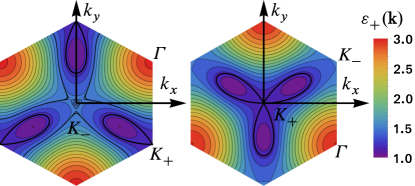
Figure 1: Under appropriate tuning of the staggered chemical potential [$M=\pm M^{\,}_{0}$ with $M^{\,}_{0}$ defined in Eq. (17b) with $t^{\,}_{1}=1$ and $t^{\,}_{2}=1/4$], Hamiltonian (10) can be made to host a monkey-saddle singularity at either one of the $\bm{K}^{\,}_{\pm}$ points. While the constant-energy contours of the monkey-saddle dispersion (1) are open, those in the Haldane model in panels (a) and (b) are closed due to the correction of order $\propto\bm{k}^{4}$ to the monkey-saddle dispersion (1). The monkey saddle with its singular energy contour that is shaped like the boundary of a three-leaf clover (bold and black) is here realized at $\bm{K}^{\,}_{+}$, while a simple maximum is realized at $\bm{K}^{\,}_{-}$ higher up in energy.

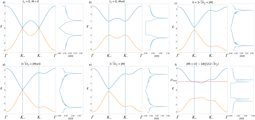
Figure 2: Dispersions (11b) and density of states (DOS) $\nu(\varepsilon)\>=N^{-2}\sum_{\pm}\sum_{\bm{k}}\delta\big{(}\varepsilon-\varepsilon^{\,}_{\pm}(\bm{k})\big{)}$ for the single-particle tight-binding Hamiltonian (10). The choice $N=1001$ is made and each delta function entering the DOS is regularized by a normalized Gaussian of variance $\sigma^{2}_{\mathrm{Gaussian}}\sim N^{-2}$. Under tuning of parameters, where we set $t^{\,}_{1}=1$, Hamiltonian (10) displays changes in both the band geometry and the band topology. We seek to obtain a monkey saddle at $\bm{K}^{\,}_{+}$ with an extremum at $\bm{K}^{\,}_{-}$, located higher up in energy, in the upper band of Hamiltonian (10). Such a phase is automatically in the topological regime with nonvanishing Chern numbers for each filled band. This phase can be reached starting from the gapless, and time-reversal invariant Dirac semimetal in (a). As a staggered chemical potential ($M$) is turned on, a gap at both the $\bm{K}^{\,}_{\pm}$ points appears as depicted in (b). The dispersions in the neighborhoods of $\bm{K}^{\,}_{+}$ and $\bm{K}^{\,}_{-}$ are symmetric because of time-reversal symmetry. In (c), a small time-reversal breaking next-nearest-neighbor hopping $t^{\,}_{2}$ that causes an asymmetry between the dispersion around $\bm{K}^{\,}_{+}$ and that around $\bm{K}^{\,}_{-}$ is turned on. As the strength of $t^{\,}_{2}$ is increased to $|M|/3\sqrt{3}$, the gap at $\bm{K}^{\,}_{+}$ closes, as in (d). By increasing $t^{\,}_{2}$ further as in (e), the topological regime with nonvanishing Chern number is entered. Finally, increasing $t^{\,}_{2}$ to satisfy the condition $M=(t^{2}_{1}-18\,t^{2}_{2})/(2\sqrt{3}\,t^{\,}_{2})$, we obtain a monkey saddle at $\bm{K}^{\,}_{+}$ and a simple maxima at $\bm{K}^{\,}_{-}$, higher in energy. This is depicted in (f). The van Hove singularities in the DOS of panels (a)–(e) have become monkey-saddle singularities at $\bm{K}^{\,}_{+}$ and van Hove singularities at $\bm{K}^{\,}_{-}$ in panel (f).

Assuming that $M$ has been tuned to either $M^{\,}_{0}$ or $-M^{\,}_{0}$, so as to obtain the monkey saddle at $\bm{K}^{\,}_{+}$ or $\bm{K}^{\,}_{-}$, respectively, we examine the sign of $|M^{\,}_{0}|-3\sqrt{3}\,|t^{\,}_{2}|$. If it is negative, then we are in the regime for which the Chern number is nonvanishing and the band is topological. We have

$$|M^{\,}_{0}|-3\sqrt{3}\,|t^{\,}_{2}|=\frac{18\,t^{2}_{2}-t^{2}_{1}}{2\sqrt{3}\,|t^{\,}_{2}|}-3\sqrt{3}\,|t^{\,}_{2}|=\frac{-t^{2}_{1}}{2\sqrt{3}\,|t^{\,}_{2}|}<0.$$ (21)

Thus, if we tune the chemical potential to the energy (19a) of the monkey saddle and assume that the energy of the local extremum (19b) is larger, i.e., Eq. (19c) holds, then the two bands necessarily have nonvanishing Chern numbers.

We plot in Fig. 2 the two single-particle dispersions (11) along the cuts $\Gamma-K^{\,}_{+}-K^{\,}_{-}-\Gamma$ in the Brillouin zone for different values of $M$ and $t^{\,}_{2}$, holding $t^{\,}_{1}$ fixed. Panel (a) corresponds to the case with two inequivalent Dirac points at which the upper and lower bands touch. Panel (b) corresponds to a gap at the two Dirac points of panel (a) induced by the staggered chemical potential $M$. Panel (c) shows the effect on panel (b) of a small $t^{\,}_{2}$. The spectral valley symmetry is broken. In panel (d), the competition between $M$ and $t^{\,}_{2}$ results in a gap-closing transition at one of the Dirac points from panel (a). In panel (e) the gap reopens as $t^{\,}_{2}$ dominates over $M$. The bands now have the Chern numbers $\pm 1$. In panel (f), $K^{\,}_{+}$ realizes a monkey saddle, while $K^{\,}_{-}$ realizes a local extremum.

We remark that a non-vanishing Hall conductivity results from breaking time-reversal symmetry. The anomalous Hall conductivity contribution from the partially filled band varies continuously as a function of the band filling. This contribution can be expressed as an integral over the Brillouin zone of the (regular) Berry curvature over the filled states. While this integral is continuous as a function of the chemical potential as the latter is varied across the monkey-saddle singularity, derivatives of the Hall conductivity with respect to the chemical potential will inherit the singularities in the DOS.

III The effects of interactions on a Monkey saddle

We consider a two-dimensional gas of spinful electrons whose single-particle and spin-degenerate dispersion

$$\varepsilon^{\,}_{\mathrm{ms}}(\bm{k})=-\varepsilon^{\,}_{\mathrm{ms}}(-\bm{k})$$ (22)

is the monkey-saddle dispersion defined by Eq. (1). The number of energy eigenvalues per unit area in the interval $(\varepsilon,\varepsilon+\mathrm{d}\varepsilon)$ defines the monkey-saddle density of states

$$\nu^{\,}_{\mathrm{ms}}(\varepsilon):=\int\frac{\mathrm{d}^{2}\bm{k}}{(2\pi)^{2}}\ \delta\Big{(}\varepsilon-\varepsilon(\bm{k})\Big{)}.$$ (23a)

It is given by  [9]

$$\nu^{\,}_{\mathrm{ms}}(\varepsilon)=\frac{1}{2\pi^{3/2}}\,\frac{\Gamma(1/6)}{\Gamma(2/3)}\,E^{-2/3}\,|\varepsilon|^{-1/3}.$$ (23b)

As emphasized in Ref. 9, it displays a power-law singularity at the singular energy $\varepsilon=0$.

This non-interacting electron gas is perturbed by a contact density-density interaction for opposite spins. The quantum dynamics is thus governed by the many-body Hamiltonian

$$\widehat{H}:=\widehat{H}^{\,}_{\mathrm{ms}}+\widehat{H}^{\,}_{\mathrm{int}},$$ (24a)

where the kinetic energy is given by

$$\widehat{H}^{\,}_{\mathrm{ms}}:=\sum_{\sigma=\uparrow,\downarrow}\ \int\limits_{|\varepsilon(\bm{k})|\leq\Lambda}\mathrm{d}^{2}\bm{k}\ \hat{c}^{{\dagger}}_{\sigma}(\bm{k})\left[\varepsilon^{\,}_{\mathrm{ms}}(\bm{k})-\mu\right]\hat{c}^{\,}_{\sigma}(\bm{k})$$ (24b)

and the interaction is given by

$$\widehat{H}^{\,}_{\mathrm{int}}:=g\,\int\mathrm{d}^{2}\bm{r}\,\hat{c}^{{\dagger}}_{\uparrow}(\bm{r})\,\hat{c}^{\vphantom{{\dagger}}}_{\uparrow}(\bm{r})\,\hat{c}^{{\dagger}}_{\downarrow}(\bm{r})\,\hat{c}^{\vphantom{{\dagger}}}_{\downarrow}(\bm{r}).$$ (24c)

Here, we have introduced an ultraviolet energy cutoff $$\Lambda \bm{k}^{4} \bm{k}^{3} \mu g g$$, corresponding to the energy scale at which corrections of order in any lattice regularization of the dispersion (1) are comparable to the contribution, denotes the chemical potential, and measures the strength of the contact interaction (a positive penalizes local double occupancy by electrons). The electronic field operators obey fermionic equal-time anti-commutation relations, i.e., the only nonvanishing equal-time anti-commutators are

$$\left\{\hat{c}^{\vphantom{{\dagger}}}_{\sigma\vphantom{\sigma^{\prime}}}(\bm{r}),\hat{c}^{{\dagger}}_{\sigma^{\prime}}(\bm{r}^{\prime})\right\}=\delta^{\,}_{\sigma,\sigma^{\prime}}\,\delta(\bm{r}-\bm{r}^{\prime}),$$ (24d)

$$\left\{\hat{c}^{\vphantom{{\dagger}}}_{\sigma\vphantom{\sigma^{\prime}}}(\bm{k}),\hat{c}^{{\dagger}}_{\sigma^{\prime}}(\bm{k}^{\prime})\right\}=\delta^{\,}_{\sigma,\sigma^{\prime}}\,\delta(\bm{k}-\bm{k}^{\prime}).$$ (24e)

The chemical potential is fixed by the number $N^{\,}_{\mathrm{e}}$ of electrons in the large area $A$. Henceforth, we set the units such that

$$\hbar=1,\quad k^{\,}_{\mathrm{B}}=1,$$ (25a)

for the Planck and Boltzmann constants, respectively. In these units, temperature $$T \beta=1/T$$ has units of energy and time has units of inverse energy. The grand-canonical partition function at the inverse temperature is

$$Z(\beta,\mu):=\mathrm{Tr}\,e^{-\beta\widehat{H}},\qquad N^{\,}_{\mathrm{e}}=\beta^{-1}\,\left(\frac{\partial\,\ln Z}{\partial\,\mu}\right)(\beta,\mu).$$ (25b)

The decay rate $\Gamma(g,T)$ of quasi-particles when $\mu=0$ arising from the contact interaction was calculated in Ref. 9 to the first non-trivial order in perturbation theory. It is given by

$$\Gamma(g,T)=C\ g^{2}\ \nu^{2}(T)\,T\sim T^{1/3}$$ (26)

with $C$ a positive numerical constant (that is calculated in the limit $\Lambda\to\infty$). For comparison, the decay rate of a Fermi liquid in two-dimensional space scales with temperature as $T^{2}$ up to a multiplicative logarithmic correction. However, this non-Fermi-liquid decay rate does not hold all the way to vanishing temperature as higher-order corrections in perturbation theory in powers of $g$ acquire power-law corrections in the temperature with negative scaling exponents, since the dimensionless expansion parameter is $g\,\nu(T)$.

Renormalization-group techniques can be useful when perturbation theory is not converging uniformly. After tracing over all electrons whose energies are within the energy shell $\Lambda-\mathrm{d}\Lambda\leq|\varepsilon^{\,}_{\mathrm{ms}}(\bm{k})|\leq\Lambda$ with

$$\frac{\mathrm{d}\Lambda}{\Lambda}=\mathrm{d}\ell,$$ (27)

infinitesimal, it is possible to preserve the form invariance of the grand-canonical partition function provided the dimensionless temperature

$$\overline{T}:=\frac{T}{\Lambda},$$ (28a)

the dimensionless chemical potential

$$\overline{\mu}:=\frac{\mu}{\Lambda},$$ (28b)

and the dimensionless interaction strength

$$\overline{g}:=\nu(\Lambda)\,g,$$ (28c)

obey the renormalization-group (RG) equations

$$\frac{\mathrm{d}\,\overline{T}}{\mathrm{d}\,\ell}=\overline{T},$$ (29a)

$$\frac{\mathrm{d}\,\overline{\mu}}{\mathrm{d}\,\ell}=\left[1-\frac{\overline{g}}{2\overline{T}\,\cosh^{2}\left(\frac{1}{2\overline{T}}\right)}\right]\overline{\mu},$$ (29b)

$$\frac{\mathrm{d}\,\overline{g}}{\mathrm{d}\,\ell}=\frac{1}{3}\,\overline{g}.$$ (29c)

These RG equations were derived perturbatively about the fixed point

$$\overline{T}^{\,\star}=\overline{\mu}^{\,\star}=\overline{g}^{\,\star}=0$$ (30)

up to order $\bar{g}^{3}$ in Refs. 9 and 15. Whereas $\overline{T}$ and $\overline{g}$ flow to strong coupling, i.e., beyond the range of validity of these perturbative RG flows, the beta function of the dimensionless chemical potential $\overline{\mu}$ undergoes a sign change if and only if the initial value of $\overline{g}$ is larger than the initial value of $2\overline{T}\,\cosh^{2}\left(\frac{1}{2\overline{T}}\right)$. If the initial conditions correspond to vanishing temperature, the RG equations (29) simplify to

$$\frac{\mathrm{d}\,\overline{\mu}}{\mathrm{d}\,\ell}=\overline{\mu},\qquad\frac{\mathrm{d}\,\overline{g}}{\mathrm{d}\,\ell}=\frac{1}{3}\,\overline{g}.$$ (31a)

If the initial conditions correspond to vanishing chemical potential the RG equations (29) simplify to

$$\frac{\mathrm{d}\,\overline{T}}{\mathrm{d}\,\ell}=\overline{T},\qquad\frac{\mathrm{d}\,\overline{g}}{\mathrm{d}\,\ell}=\frac{1}{3}\,\overline{g}.$$ (31b)

One possible interpretation of this RG flow to strong coupling is a Stoner instability to an itinerant ferromagnetic phase, as can be confirmed by a mean-field analysis  [15]. Pomeranchuk instabilities (area-preserving deformations of the three-leaf clover Fermi surface into either a single Fermi surface enclosing the monkey-saddle singularity at $\bm{K}^{\,}_{+}$, say, or three disconnected Fermi surfaces that do not enclose the monkey-saddle singularity) are also possible. Any superconducting instability must be of the Fulde-Ferrell-Larkin-Ovchinnikov (FFLO) type with the characteristic monkey-saddle wave vector $\bm{K}^{\,}_{+}$, say. More exotic instabilities such as a fractional Chern insulator when the band hosting the monkey saddle has a nonvanishing Chern number, the filling fraction is 1/3 at the monkey saddle, and the interaction strength is larger than the band width, say, cannot be ruled out owing to the DOS at the monkey saddle. Nonperturbative techniques are needed to establish the fate of the monkey saddle when perturbed by a contact interaction.

We are going to use the mean-field approximation to argue that the monkey-saddle singularity is unstable when we elevate the spinless fermions in Hamiltonian (10) to electrons with spin-1/2 and add an on-site repulsive Hubbard interaction with coupling $U>0$ and a next-nearest-neighbor repulsive interaction with coupling $V>0$.

For the case of a two-dimensional gas of spinless electrons, there is no quartic density-density contact interaction as in Eq. (24c). The lowest-order interaction term that we may add is

$$\propto[\hat{c}^{\dagger}(\bm{r})\,\bm{\nabla}\hat{c}(\bm{r})]^{2}.$$ (32)

This interaction is irrelevant by power counting and is thus not expected to destabilize the monkey saddle for small values of its coupling. Accordingly, we are going to show that a monkey-saddle singularity can be stabilized by fine-tuning lattice parameters in the presence of repulsive nearest-neighbor interactions within a mean-field approximation.

IV Mean-field analysis

In this section, we analyze the stability of the monkey-saddle singularity in the spectrum of the Hamiltonian (10) against short-range interactions at the mean-field level. We treat the cases of spinful and spinless electrons separately. For the former case, we consider repulsive on-site Hubbard and nearest-neighbor interactions. For the latter case, we only consider a repulsive nearest-neighbor interaction.

IV.1 Spinful case

We presume Hamiltonian (10) for spinful electrons fine-tuned to a monkey saddle located at $\bm{K}^{\,}_{+}$ in the upper ($+$) band that is perturbed by a repulsive on-site Hubbard interaction of strength $U$ and a repulsive nearest-neighbor interaction of strength $V$, given by

$$\widehat{H}^{\,}_{U}=U\sum_{\bm{r}\in\Lambda}\Big{(}\hat{n}^{\,}_{\mathrm{A},\uparrow,\bm{r}}\,\hat{n}^{\,}_{\mathrm{A},\downarrow,\bm{r}}+\hat{n}^{\,}_{\mathrm{B},\uparrow,\bm{r}+\bm{a}^{\,}_{1}}\,\hat{n}^{\,}_{\mathrm{B},\downarrow,\bm{r}+\bm{a}^{\,}_{1}}\Big{)},$$ (33a)

$$\widehat{H}^{\,}_{V}=V\sum_{\bm{r}\in\Lambda}\sum_{i=1}^{3}\hat{n}^{\,}_{\mathrm{A},\bm{r}}\,\hat{n}^{\,}_{\mathrm{B},\bm{r}+\bm{a}^{\,}_{i}},$$ (33b)

respectively. Here, we denote with $\Lambda$ the triangular Bravais lattice hosting the A sites. The honeycomb lattice is made of $|\Lambda|$ unit cells, each one containing two sites labeled by A and B. The total number of sites in the honeycomb lattice is thus $2|\Lambda|$. Hereby, we have introduced the spin and position resolved fermion number operators

$$\hat{n}^{\,}_{\mathrm{A},\sigma,\bm{r}}=\hat{c}^{\dagger}_{\mathrm{A},\sigma,\bm{r}}\hat{c}^{\,}_{\mathrm{A},\sigma,\bm{r}},\quad\hat{n}^{\,}_{\mathrm{B},\sigma,\bm{r}+\bm{a}^{\,}_{i}}=\hat{c}^{\dagger}_{\mathrm{B},\sigma,\bm{r}+\bm{a}^{\,}_{i}}\hat{c}^{\,}_{\mathrm{B},\sigma,\bm{r}+\bm{a}^{\,}_{i}},$$ (34a)

$$\hat{n}^{\,}_{\mathrm{A},\bm{r}}=\sum_{\sigma=\pm}\hat{n}^{\,}_{\mathrm{A},\sigma,\bm{r}},\quad\hat{n}^{\,}_{\mathrm{B},\bm{r}+\bm{a}^{\,}_{i}}=\sum_{\sigma=\pm}\hat{n}^{\,}_{\mathrm{B},\sigma,\bm{r}+\bm{a}^{\,}_{i}},$$ (34b)

where $$\hat{c}^{{\dagger}}_{\mathrm{A},\sigma,\bm{r}} \hat{c}^{{\dagger}}_{\mathrm{B},\sigma,\bm{r}+\bm{a}^{\,}_{i}} \sigma \bm{r} \bm{r}+\bm{a}^{\,}_{i}$$ and create an electron with spin on the A and B sublattices at positions and , respectively.

We employ five mean-field order parameters: the uniform charge density $n^{\,}_{\mathrm{e}}$, the uniform magnetization density $\overline{m}$, and the three uniform, directed, nearest-neighbor bond density order parameters $\overline{\chi}^{\,}_{i}$. These five order parameters are defined as the ground-state expectation values of the local operators

$$\hat{n}^{\,}_{\bm{r}}=\hat{n}^{\,}_{\mathrm{A},\bm{r}}+\hat{n}^{\,}_{\mathrm{B},\bm{r}+\bm{a}^{\,}_{1}},$$ (35a)

$$\hat{m}^{\,}_{\bm{r}}=\sum_{\sigma=\pm}\sigma\,\left(\hat{n}^{\,}_{\mathrm{A},\sigma,\bm{r}}+\hat{n}^{\,}_{\mathrm{B},\sigma,\bm{r}+\bm{a}^{\,}_{1}}\right),$$ (35b)

$$\hat{\chi}^{\,}_{i,\sigma,\sigma^{\prime},\bm{r}}=\hat{c}^{\dagger}_{\mathrm{A},\sigma,\bm{r}}\,\hat{c}^{\,}_{\mathrm{B},\sigma^{\prime},\bm{r}+\bm{a}^{\,}_{i}}+\mathrm{H.c.},$$ (35c)

respectively. We make the mean-field Ansatz

$$\left\langle\hat{n}^{\,}_{\bm{r}}\,\right\rangle=n^{\,}_{\mathrm{e}},$$ (36a)

$$\left\langle\hat{m}^{\,}_{\bm{r}}\,\right\rangle=\overline{m},$$ (36b)

$$\left\langle\hat{\chi}^{\,}_{i,\sigma,\sigma^{\prime},\bm{r}}\,\right\rangle=\delta^{\,}_{\sigma\,\sigma^{\prime}}\,\left(\overline{\chi}+\delta^{\,}_{i,1}\,\overline{\chi}^{\,}_{1}\right),$$ (36c)

where $\left\langle\cdots\right\rangle$ denotes the expectation value over the mean-field ground state. In the mean-field Ansatz (36), we assume that the order parameters are independent of the position $\bm{r}$, i.e., the Ansatz (36) does not include charge-density, spin-density, or bond-density waves. This assumption is justified since (i) the single-particle energies at $\bm{K}^{\,}_{+}$ and $\bm{K}^{\,}_{-}$ are separated in energy (ii) and there are no momentum-conserving nesting vectors that connect two points from the Fermi surface when the chemical potential is tuned close to the monkey-saddle energy. Consequently, there is no band folding in the Brillouin zone and the mean-field ground state remains metallic for any noninteger filling fraction.

The mean-field Ansatz (36a) for the charge density fixes the chemical potential such that the filling fraction of the interacting system coincides with that of the noninteracting model. The mean-field Ansatz (36b) assumes a ferromagnetic ground state whenever $|\overline{m}|>0$ for which the spin-rotation symmetry is spontaneously broken [time-reversal symmetry is explicitly broken in the Hamiltonian (10) by the next-nearest neighbor hopping term (10d)]. The mean-field Ansatz (36c) assumes a uniform bond-density order parameter $\overline{\chi}$ that does not break the $\mathbb{Z}^{\,}_{3}$-rotation symmetry that is modulated by $\overline{\chi}^{\,}_{1}$ along the $\bm{a}^{\,}_{1}$ direction. Any nonvanishing $|\overline{\chi}^{\,}_{1}|$ breaks the $\mathbb{Z}^{\,}_{3}$-rotation symmetry spontaneously, while preserving the reflection symmetry along the $\bm{a}^{\,}_{1}$ direction.

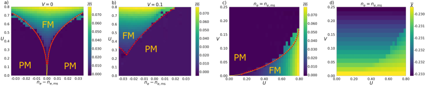
Figure 3: The mean-field phase diagram at zero temperature in the coupling space spanned by the filling fraction $n^{\,}_{e}$, the on-site repulsive interaction $U$, and the nearest-neighbor repulsive interaction $V$ is obtained from solving numerically the mean-field equations (38) (All energies are measured in units of $t^{\,}_{1}$.). Dashed red lines show the approximate phase boundaries in panels (a), (b), and (c). The yellow solid lines shows the approximate phase boundaries in the thermodynamic limit in panels (a) and (c). (a) Two-dimensional cut for the values taken by $\overline{m}$ when $V=0$ in units of $t^{\,}_{1}$. A Stoner instability towards itinerant ferromagnetism takes place for any nonvanishing Hubbard interaction $U>U^{\,}_{\mathrm{c}}$ for given $n^{\,}_{e}$. The minimum value $U^{\,}_{\mathrm{c},\mathrm{min}}$ taken by $U^{\,}_{\mathrm{c}}$ occurs for $n^{\,}_{e}=n^{\,}_{e,\mathrm{ms}}$. The nonvanishing value of $U^{\,}_{\mathrm{c},\mathrm{min}}$ above which ferromagnetism is established when the filling fraction is fine tuned to the monkey saddle, i.e., $n^{\,}_{e}=n^{\,}_{e,\mathrm{ms}}$, is due to a finite-size effect that cuts off the diverging DOS. In the thermodynamic limit, $U^{\,}_{\mathrm{c},\mathrm{min}}\to 0$ at $n^{\,}_{e}=n^{\,}_{e,\mathrm{ms}}$. (b) Two-dimensional cut for the values taken by $\overline{m}$ when $V=0.1$ in units of $t^{\,}_{1}$. A nonvanishing $V>0$ has two effects. It increases the minimum value of $U^{\,}_{\mathrm{c}}$ from panel (a) to a value that remains nonvanishing in the thermodynamic limit. The position of the minimum value of $U^{\,}_{\mathrm{c}}$ from panel (a) is shifted along the $n^{\,}_{e}$ axis. (c) Two-dimensional cut for the values taken by $\overline{m}$ when $n^{\,}_{e}=n^{\,}_{e,\mathrm{ms}}$. The critical value $U^{\,}_{\mathrm{c}}$ above which ferromagnetism sets in is an increasing function of $V$. (d) Two-dimensional cut for the values taken by $\overline{\chi}$ when $n^{\,}_{e}=n^{\,}_{e,\mathrm{ms}}$. The value of $\overline{\chi}$ is nonvanishing everywhere.

After performing the mean-field approximation, the dispersions (11) become

$$\overline{\varepsilon}^{\,}_{\tau,\sigma,\bm{k}}=\tau\,\overline{\varepsilon}^{\,}_{\bm{k}}-\frac{1}{2}\sigma\,U\,\overline{m},$$ (37a)

with

$$\overline{\varepsilon}^{\,}_{\bm{k}}=\sqrt{M^{2}_{\bm{k}}+\left|\Phi^{\,}_{\bm{k}}\right|^{2}},$$ (37b)

$$M^{\,}_{\bm{k}}=M+2\,t^{\,}_{2}\sum_{i=1}^{3}\sin(\bm{k}\cdot\bm{b}_{i}),$$ (37c)

$$\Phi^{\,}_{\bm{k}}=\sum\limits_{i=1}^{3}\overline{t}^{\,}_{1,i}\,e^{+\mathrm{i}\bm{k}\cdot\bm{a}^{\,}_{i}},$$ (37d)

$$\overline{t}^{\,}_{1,i}=\begin{cases}t^{\,}_{1}-V\,\left(\overline{\chi}+\overline{\chi}^{\,}_{1}\right),&i=1,\\ &\\ t^{\,}_{1}-V\,\overline{\chi},&i=2,3,\end{cases}$$ (37e)

where $\tau=\pm$ is the band index and $\sigma=\pm$ is the spin index. The self-consistent mean-field equations corresponding to the Ansatz (36) are

$$n^{\,}_{e}=\frac{1}{|\Lambda|}\sum_{\bm{k},\tau,\sigma}f^{\,}_{\mathrm{FD}}\left(\overline{\varepsilon}^{\,}_{\tau,\sigma,\bm{k}}-\overline{\mu}\right),$$ (38a)

$$\overline{m}=\frac{1}{|\Lambda|}\sum_{\bm{k},\tau,\sigma}\sigma\,f^{\,}_{\mathrm{FD}}\left(\overline{\varepsilon}^{\,}_{\tau,\sigma,\bm{k}}-\overline{\mu}\right),$$ (38b)

$$\overline{\chi}=\frac{1}{2|\Lambda|}\sum_{\bm{k},\tau,\sigma}\tau\mathrm{Re}\left\{e^{\mathrm{i}\bm{k}\cdot\bm{a}^{\,}_{2}}\,\frac{\Phi^{*}_{\bm{k}}}{2\,\overline{\varepsilon}^{\,}_{\bm{k}}}\right\}f^{\,}_{\mathrm{FD}}\left(\overline{\varepsilon}^{\,}_{\tau,\sigma,\bm{k}}-\overline{\mu}\right),$$ (38c)

$$\overline{\chi}^{\,}_{1}=\frac{1}{2|\Lambda|}\sum_{\bm{k},\tau,\sigma}\tau\mathrm{Re}\left\{e^{\mathrm{i}\bm{k}\cdot\bm{a}^{\,}_{1}}\frac{\Phi^{*}_{\bm{k}}}{2\,\overline{\varepsilon}^{\,}_{\bm{k}}}\right\}f^{\,}_{\mathrm{FD}}\left(\overline{\varepsilon}^{\,}_{\tau,\sigma,\bm{k}}-\overline{\mu}\right)-\overline{\chi}.$$ (38d)

Here, the Fermi-Dirac distribution is

$$f^{\,}_{\mathrm{FD}}(\epsilon):=\begin{cases}\frac{1}{e^{\epsilon/T}+1},&T>0\\ &\\ \Theta(-\epsilon),&T=0,\end{cases}$$ (39)

where $T$ is the temperature (in the units with the Boltzmann constant set to unity), and $\Theta(x)$ is the step function equal to $1$ for positive $x$ and $0$ otherwise. The chemical potential $\overline{\mu}$ is determined by solving self-consistency equation (38a) where the charge density $n^{\,}_{e}$ is that of the noninteracting Hamiltonian (10). We denote by $\mu^{\,}_{e}$ the chemical potential that delivers the charge density $n^{\,}_{e}$ for the noninteracting dispersion. We note that mean-field Ansatz (36c) assumes that the bond-density order parameter is the same for the $\bm{a}^{\,}_{2}$- and $\bm{a}^{\,}_{3}$-directions. Therefore, in the self-consistency equations (38c) and (38d), we could have equivalently chosen $\bm{a}^{\,}_{3}$ instead of $\bm{a}^{\,}_{2}$. One can also generalize Ansatz (36c) by introducing three separate bond-density order parameters, one for each direction $\bm{a}^{\,}_{i}$. Such a more general mean-field Ansatz, while being computationally heavier, does not change our results within the investigated parameter range.

The self-consistent mean-field equation (38) consists of four unknowns, $\left\{\overline{\mu},\,\overline{m},\,\overline{\chi},\,\overline{\chi}^{\,}_{1}\right\}$ that are to be determined as a function of three parameters $\left\{n^{\,}_{e},\,U,\,V\right\}$. We have solved Eqs. (38) numerically on the Brillouin zone $\Omega^{\,}_{\mathrm{BZ}}$ discretized on a $501\times 501$ grid of $\bm{k}$-points. All energy scales are measured in units of $t^{\,}_{1}$. We have set $t^{\,}_{2}=0.25$ and $M=M^{\,}_{0}$ for which a monkey-saddle singularity appears. We consider repulsive couplings $U\geq 0$ and $V\geq 0$. The coupling $V$ is taken to be smaller than the energy difference in the upper band between the monkey saddle at $\bm{K}^{\,}_{+}$ and the local extremum $\mu^{\,}_{\mathrm{le}}$ at $\bm{K}^{\,}_{-}$. For our choice of parameters, this difference is $\Delta\mu=\mu^{\,}_{\mathrm{le}}-\mu^{\,}_{\mathrm{ms}}\approx 0.29$ in units of $t^{\,}_{1}$. For interaction strengths larger than $\Delta\mu$, a bond-density wave with a nonzero wave vector is a potential instability that is not contained in the Ansatz (36).

In Fig. 3, the mean-field solutions for the order parameters $\overline{m}$ and $\overline{\chi}^{\,}$ are shown as functions of the parameters $n^{\,}_{e}$, $U$, and $V$. We only find two phases, an itinerant phase supporting ferromagnetism ($\overline{m}\neq 0$) and an itinerant phase that is paramagnetic ($\overline{m}=0$). The phase boundaries are shown by red dashed lines. Within the parameter space of interest, we do not find the signature of a Pomeranchuk instability ($\overline{\chi}^{\,}_{1}\neq 0$) that would break spontaneously the lattice $\mathbb{Z}^{\,}_{3}$-rotation symmetry. Nevertheless, the monkey-saddle singularity is unstable against any finite repulsive, nearest-neighbor interaction $V$ as we shall explain shortly.

For $V=0$, we find that the Stoner instability destroys the monkey-saddle singularity for any repulsive Hubbard interaction strength $U>0$ when the filling fraction is tuned to be at the monkey saddle ($n^{\,}_{e}=n^{\,}_{e,\mathrm{ms}}$). This is signaled by (i) the nonvanishing magnetization density $\overline{m}$ in Fig. 3(a) for $U\geq U^{\,}_{\mathrm{c}}$ where for any finite lattice size $|\Lambda|$ the critical interaction strength $U^{\,}_{\mathrm{c}}$ is minimized as a function of $n^{\,}_{e}$ when $n^{\,}_{e}=n^{\,}_{e,\mathrm{ms}}$ (ii) whereby we have verified that this minimum $U^{\,}_{\mathrm{c},\mathrm{min}}$ of $U^{\,}_{\mathrm{c}}$ decreases with increasing lattice size $|\Lambda|$ with the extrapolated limit $U^{\,}_{\mathrm{c},\mathrm{min}}\to 0$ as $|\Lambda|\to\infty$. This mean-field calculation thus confirms the intuition based on Sec. III that the flow of the on-site interaction to strong coupling is a diagnostic of a Stoner instability (an itinerant Fermi-liquid phase supporting ferromagnetic long-range order) as opposed to a featureless (without any long-range order) non-Fermi-liquid phase. The corresponding effect on the mean-field DOS is shown in Fig.  4(a). The mean-field treatment of the on-site repulsive interaction only changes the spin-resolved chemical potentials. This will not affect the non-interacting DOS at values of $n^{\,}_{\mathrm{e}}-n^{\,}_{\mathrm{e,ms}}$ for which the non-interacting DOS is too small to induce a Stoner instability. However, a Stoner instability must happen close enough to the monkey-saddle filling fraction $n^{\,}_{\mathrm{e,ms}}$ for any non-vanishing value of $U>0$, thereby cutting off the monkey-saddle divergence of the noninteracting DOS at the monkey-saddle filling fraction. Correspondingly, the regularized mean-field DOS shows the double-peak shape from Fig. 4(a).

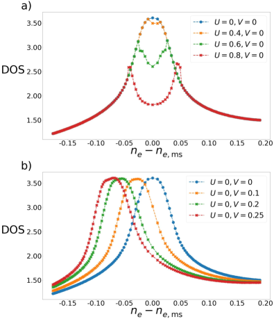
Figure 4: The regularized mean-field DOS as a function of the deviation $n^{\,}_{\mathrm{e}}-n^{\,}_{\mathrm{e,ms}}$ of the filling fraction $n^{\,}_{\mathrm{e}}$ from the monkey-saddle filling fraction $n^{\,}_{\mathrm{e,ms}}$ is plotted for different values of the interaction strengths $U\geq 0$ and $V\geq 0$. The $\delta$-functions in the mean-field DOS are regularized by normalized Gaussians of variance $\sigma^{2}_{\mathrm{Gaussian}}\sim 10/N^{2}$ with $N=501$. In panel (a), $U$ is increased holding $V=0$. The single regularized peak in the noninteracting DOS is split into two peaks by a nonvanishing $U$. Contrary to the height of the monkey-saddle peak of the regularized noninteracting DOS, the height of these secondary peaks remains finite in the limit $\sigma^{\,}_{\mathrm{Gaussian}}\to 0$. In panel (b), $V$ is increased holding $U=0$. The single peak in the regularized noninteracting DOS is translated to the left by a nonvanishing $V$. This observation can be explained by $V>0$ inducing quadratic perturbations to the monkey-saddle dispersion (1) at the mean-field level. These quadratric perturbations turn the monkey-saddle singularity into a central local extremum surrounded by three van Hove saddle singularities.

Turning on a nonvanishing $V$ has two effects shown in Figs. 3(b) and 3(c). First, the value of $U^{\,}_{\mathrm{c}}$ above which ferromagnetism takes place is larger for $V=0.1$ than for $V=0$ (measured in units of $t^{\,}_{1}$) and this value remains nonvanishing in the thermodynamic limit. Second, the minimal value $U^{\,}_{\mathrm{c},\mathrm{min}}$ of $U^{\,}_{\mathrm{c}}$ in Fig. 3(b) is found at a filling fraction $n^{\,}_{e,\mathrm{min}}<n^{\,}_{e,\mathrm{ms}}$. Both effects can be understood as the renormalization (37e) of the nearest-neighbor hopping amplitude $t^{\,}_{1}$ for any nonvanishing $V$. Indeed, the uniform bond density $\overline{\chi}$ defined in Eq. (38c) is nonvanishing for any interaction strengths $U$ and $V$, and for any filling fraction except for the completely filled ($n^{\,}_{e}=4$) or completely empty ($n^{\,}_{e}=0$) bands. Any finite interaction strength $V$ thus results in corrections proportional to $k^{2}$ in the expansion (17) that had been set to $0$ by fine tuning the value of the staggered chemical potential $M$ to $M^{\,}_{0}$ so as to obtain the bare monkey-saddle dispersion (18). Under the $k^{2}$-perturbation, the monkey-saddle singularity turns into a central local extremum surrounded by three van Hove saddle singularities with dispersions $\sim k^{2}_{x}-k^{2}_{y}$ [9]. Consequently, the monkey-saddle singularity disappears through a Lifshitz transition by which the topology of the Fermi surface changes. This renormalization has two effects. It moves the position of the maximum of the mean-field DOS (i.e., the position of the minimum $U^{\,}_{\mathrm{c},\mathrm{min}}$) to a value $n^{\,}_{e,\mathrm{min}}<n^{\,}_{e,\mathrm{ms}}$ [see Fig.  4(b)]. It regularizes the diverging monkey-saddle DOS to a large but finite value at the filling fraction $n^{\,}_{e}=n^{\,}_{e,\mathrm{ms}}$ [see Fig.  4(b)]. Figure 3(c) shows the suppression of the critical interaction strength $U^{\,}_{\mathrm{c}}$ at the monkey-saddle singularity with increasing $V$. Figure 3(d) demonstrates that the uniform bond-density $\overline{\chi}$ is nonvanishing in the same field of view as in Fig. 3(c). In contrast, the non-isotropic bond-density $\overline{\chi}^{\,}_{1}$ is found to be vanishing everywhere in coupling space within the numerical error bars. In other words, we did not find any evidence for a Pomeranchuk instability.

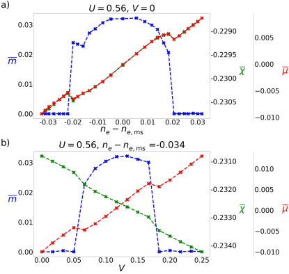
Figure 5: Dependencies of the uniform magnetization $\overline{m}$, uniform bond-density $\overline{\chi}$, and chemical potential $\overline{\mu}$ along one-dimensional cuts in coupling space at zero temperature as is explained in the text.

Figure 5 shows the variations of the uniform magnetization $\overline{m}$, the uniform bond-density wave $\overline{\chi}$, and the chemical potential $\overline{\mu}$ along one-dimensional cuts in coupling space. Figure 5(a) shows the dependence of $\overline{m}$, $\overline{\chi}$, and $\overline{\mu}$ on the electronic filling fraction $n^{\,}_{e}$ when $U=0.56$ and $V=0$ in units of $t^{\,}_{1}$. All three are discontinuous functions of $n^{\,}_{e}$ at two critical values of $n^{\,}_{e}$, one below and another above $n^{\,}_{e,\mathrm{ms}}$, for which the Stoner instability takes place. Finite-size scaling is consistent with a discontinuous dependence of $\overline{m}$ and $\overline{\chi}$ on $n^{\,}_{e}$ in the thermodynamic limit upon entering the itinerant ferromagnetic phase. The overlap of $\overline{\chi}$ and $\overline{\mu}$ is due to the fact that both are monotonically increasing functions of $n^{\,}_{e}-n^{\,}_{e,\mathrm{ms}}$ (except at their discontinuities) and their dependence can be approximated linearly for small $|n^{\,}_{e}-n^{\,}_{e,\mathrm{ms}}|\ll n^{\,}_{e,\mathrm{ms}}$. Figure 5(b) shows the dependence of $\overline{m}$, $\overline{\chi}$, and $\overline{\mu}$ on the nearest-neighbor interaction $V$ when $U=0.56$ in units of $t^{\,}_{1}$ and $n^{\,}_{e}=n^{\,}_{e,\mathrm{ms}}-0.034$. Hereto, all three are expected from finite-size scaling to be discontinuous functions of $V$ at the critical values of $V$ for which the Stoner instability takes place in the thermodynamic limit. The disappearance of the Stoner instability for large $V$ is due to the shift of the maximum of the DOS to $n^{\,}_{e,\mathrm{min}}<n^{\,}_{e,\mathrm{ms}}$ as is implied by Fig. 3(b). Increasing the values of $V$ holding $U$ and $n^{\,}_{e}$ fixed with $n^{\,}_{e}<n^{\,}_{e,\mathrm{ms}}$ is effectively changing the DOS in a nonmonotonic way. The DOS first increases, reaches a maximum, and then decreases as a function of $V$. Correspondingly, if the given values of $U$ and $n^{\,}_{e}$ are suitable in that the maximum DOS is large enough for a Stoner instability to take place, then increasing $V$ first triggers a Stoner instability followed by a re-entrant phase transition to the paramagnetic state when the DOS has decreased to a value too far from its maximum. In contrasts to Fig. 5(a), $\overline{\mu}$ is an increasing function of $V$ while $\overline{\chi}$ is a decreasing function of $V$ (except at their discontinuities). The increase in chemical potential $\overline{\mu}$ can be understood as follows. The function $-V\,\overline{\chi}$ of $V$ is monotonically increasing. Therefore, the renormalized hopping amplitude (37e) is greater than its bare value, i.e., $\overline{t}^{\,}_{1,i}>t^{\,}_{1}$. This results in an increase of both the bandwidths and the gap between the $\tau=+$ and $\tau=-$ bands in such a way that a greater $\overline{\mu}$ is required to keep the filling fraction at $n^{\,}_{e}=n^{\,}_{e,\mathrm{ms}}-0.034$.

Figure 6(a) shows the dependence of $\overline{m}$ on the on-site interaction $U$ when $V=0$ for different fixed values of $n^{\,}_{e}$. The critical value $U^{\,}_{\mathrm{c}}$ for the onset of the Stoner instability is minimal when $n^{\,}_{e}=n^{\,}_{e,\mathrm{ms}}$. It increases with the deviation $|n^{\,}_{e}-n^{\,}_{e,\mathrm{ms}}|$. Finite-size scaling is consistent with $U^{\,}_{\mathrm{c}}$ vanishing when $n^{\,}_{e}=n^{\,}_{e,\mathrm{ms}}$. When $n^{\,}_{e}\neq n^{\,}_{e,\mathrm{ms}}$, finite-size scaling is consistent with $\overline{m}$ being a discontinuous function of $U$ in the thermodynamic limit upon entering the itinerant ferromagnetic phase at $U^{\,}_{\mathrm{c}}>0$. Figure 6(b) shows the dependence of $\overline{m}$ on the on-site interaction $U$ when $n^{\,}_{e}=n^{\,}_{e,\mathrm{ms}}$ for different fixed values of $V$. The critical value $U^{\,}_{\mathrm{c}}$ for the onset of the Stoner instability is minimal when $V=0$. It increases with increasing $V$. When $V>0$, finite-size scaling is consistent with $\overline{m}$ being a discontinuous function of $U$ in the thermodynamic limit upon entering the itinerant ferromagnetic phase at $U^{\,}_{\mathrm{c}}>0$.

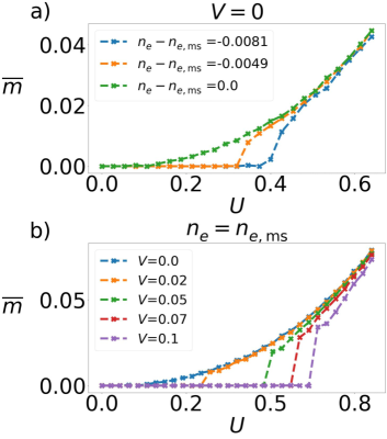
Figure 6: Dependency of the uniform magnetization $\overline{m}$ along one-dimensional cuts in coupling space at zero temperature as is explained in the text.

IV.2 Spinless Case

In Sec. IV.1, we showed for spinful electrons that the monkey-saddle singularity in the noninteracting limit is unstable against on-site Hubbard interaction at the mean-field level. We also argued that the disappearance of the monkey-saddle singularity when a repulsive nearest-neighbor interaction is present is due to the renormalization (37e) of the bare hopping amplitude $t^{\,}_{1}$. A natural question that arises is the following. Are there fine-tuned values of the couplings $t^{\,}_{1}$, $t^{\,}_{2}$, and $M$ entering the noninteracting dispersion (11) such that a monkey-saddle singularity is stabilized by a repulsive nearest-neighbor interaction treated within mean-field theory? Here, we will consider the case of spinless electrons for which the on-site Hubbard term is not present and answer this question affirmatively.

To this end, we consider the mean-field dispersion

$$\overline{\varepsilon}^{\,}_{\tau,\bm{k}}=\tau\,\overline{\varepsilon}^{\,}_{\bm{k}},$$ (40a)

with

$$\overline{\varepsilon}^{\,}_{\bm{k}}=\sqrt{M^{2}_{\bm{k}}+\left|\Phi^{\,}_{\bm{k}}\right|^{2}},$$ (40b)

$$M^{\,}_{\bm{k}}=M+2\,t^{\,}_{2}\sum_{i=1}^{3}\sin(\bm{k}\cdot\bm{b}_{i}),$$ (40c)

$$\Phi^{\,}_{\bm{k}}=\sum\limits_{i=1}^{3}\overline{t}^{\,}_{1}\,e^{+\mathrm{i}\bm{k}\cdot\bm{a}^{\,}_{i}},$$ (40d)

$$\overline{t}^{\,}_{1}=t^{\,}_{1}+\delta-V\,\overline{\chi},$$ (40e)

which is the mean-field dispersion (37) where we set $U$, $\overline{m}$, and $\overline{\chi}^{\,}_{1}$ to be zero and removed the spin index $\sigma$. Here, $\delta$ is a tunable parameter that encodes the deviations from $t^{\,}_{1}$. We retain the bare values of $t^{\,}_{2}$ and $M$ measured in units of $t^{\,}_{1}$ in the mean-field dispersion (37). Hence, when $\delta=V=0$, a monkey-saddle singularity is present in the dispersion at the filling fraction $n^{\,}_{e,\mathrm{ms}}/2$. (Here, the division by $2$ is due to the removal of half of the bands for the spinless electrons.) This is not true anymore for $\delta\neq 0$ and $V=0$ since $\overline{t}^{\,}_{1}$ differs from $t^{\,}_{1}$ so that the monkey-saddle condition $M=M^{\,}_{0}$ is not met anymore if we substitute $t^{\,}_{1}$ with $t^{\,}_{1}+\delta$ in $M^{\,}_{0}$ given by Eq. (17b). Conversely, the mean-field dispersion (40) is identical to the noninteracting dispersion (11) but with the substitution $t^{\,}_{1}\to\overline{t}^{\,}_{1}$. Because $\delta$ is only shifting the value of $\overline{t}^{\,}_{1}$ while we keep $M$ and $t^{\,}_{2}$ fixed, a monkey saddle singularity is guaranteed to exist in the spectrum only when $\overline{t}^{\,}_{1}=t^{\,}_{1}$ and at the filling fraction $n^{\,}_{e,\mathrm{ms}}/2$. With these assumptions for the mean-field dispersion, we must solve for $\overline{\mu}(V)$, $\overline{\chi}(V)$, and $\overline{\delta}(V)$ the three coupled and non-linear mean-field equations

$$n^{\,}_{e,\mathrm{ms}}=\frac{1}{|\Lambda|}\sum_{\bm{k},\tau}f^{\,}_{\mathrm{FD}}\left(\overline{\varepsilon}^{\,}_{\tau,\bm{k}}-\overline{\mu}\right),$$ (41a)

$$\overline{\chi}=\frac{1}{2|\Lambda|}\sum_{\bm{k},\tau}\tau\mathrm{Re}\left\{e^{\mathrm{i}\bm{k}\cdot\bm{a}^{\,}_{2}}\,\frac{\Phi^{*}_{\bm{k}}}{2\,\overline{\varepsilon}^{\,}_{\bm{k}}}\right\}f^{\,}_{\mathrm{FD}}\left(\overline{\varepsilon}^{\,}_{\tau,\bm{k}}-\overline{\mu}\right),$$ (41b)

$$\overline{t}^{\,}_{1,i}=t^{\,}_{1}\iff\overline{\delta}=V\,\,\overline{\chi},$$ (41c)

as a function of the repulsive nearest-neighbor interaction strength $V$. Solutions to Eq. (41) identify for which fine-tuned values $\overline{\delta}$ of the parameter $\delta$, a monkey-saddle singularity is stabilized by a repulsive nearest-neighbor interaction $V$ treated within a mean-field approximation. Notice that for any given values of the parameters $n^{\,}_{e}$, $V$, and $\delta$, Eqs. (41a) and (41b) always have a solution. However, a monkey-saddle singularity is present in the mean-field dispersion at the energy $\overline{\mu}$ only when $n^{\,}_{e}=n^{\,}_{e,\mathrm{ms}}/2$ and Eq. (41c) is satisfied.

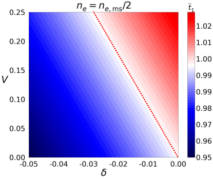
Figure 7: Renormalized hopping amplitude $\overline{t}^{\,}_{1}$ that is obtained by solving the self-consistent mean-field equations (41) at zero temperature. The red dashed line shows the points in the parameter space for which the condition (41c) is met. For any interaction strength $V$, there is a fine-tuned value $\bar{\delta}$ of $\delta$ for which an interacting monkey-saddle singularity appears in the mean-field spectrum at the filling $n^{\,}_{e}=n^{\,}_{e,\mathrm{ms}}/2$.

In Fig. 7, we fix the filling fraction to $n^{\,}_{e}=n^{\,}_{e,\mathrm{ms}}/2$ and plot the renormalized hopping amplitude $\overline{t}^{\,}_{1}$ that is obtained by solving the mean-field equations (41a) and (41b) in parameter space of $\delta$ and $V$. We find that, at the mean-field level and for any given interaction strength $0\leq V\leq 0.25$, there exists a fine-tuned value $\bar{\delta}$ of $\delta$ for which an interacting monkey-saddle singularity appears at the filling $n^{\,}_{e}=n^{\,}_{e,\mathrm{ms}}/2$. Notice that for fixed $\overline{t}^{\,}_{1}$ at the filling $n^{\,}_{e}=n^{\,}_{e,\mathrm{ms}}/2$, the solution to Eq. (41b) fixes the value of $\overline{\chi}$. Equation (40e) then implies a linear relation between $V$ and $\delta$. In other words, constant $\overline{t}^{\,}_{1}$ contours in the $V-\delta$ plane must necessarily be linear as is the case in Fig. 7. We show the linear contour for which Eq. (41c) is solved by the red dashed line in Fig. 7.

IV.3 Conclusions

To recapitulate, for the spinful electrons mean-field theory predicts that the noninteracting monkey-saddle singularity is unstable to both the repulsive on-site Hubbard interaction and the repulsive nearest-neighbor interactions for any nonvanishing values of their coupling strengths.

In the former case, a Stoner instability occurs for any nonvanishing $U$ at $n^{\,}_{e}=n^{\,}_{e,\mathrm{ms}}$, which destroys the monkey-saddle singularity by a rigid mean-field energy shift of the spin-up band relative to that of the spin-down band. Because of the itinerant ferromagnetic order, spin-rotation symmetry is spontaneously broken.

In the latter case, any finite coupling $V>0$ leads to a renormalization of the hopping amplitude $t^{\,}_{1}$ to $\overline{t}^{\,}_{1,1}=\overline{t}^{\,}_{1,2}=\overline{t}^{\,}_{1,3}>t^{\,}_{1}$. This leads to a nonvanishing $k^{2}$-correction to the monkey-saddle dispersion (11) that removes the higher-order singularity through a Lifshitz transition of the Fermi surface.

We then showed that this removal of the monkey-saddle singularity when $V>0$ can be compensated by the fine-tuning of the bare hopping amplitude $t^{\,}_{1}$ such that an interacting monkey-saddle singularity appears in the mean-field dispersion. For the spinless electrons, this fine-tuned interacting monkey-saddle singularity is stable as the on-site Hubbard interaction is inactive.

V Summary

We addressed the question of whether it is possible to obtain single odd higher-order singularities in the dispersion of an electronic system. The motivation for this search is that when singularities appear in pairs, interactions naturally lead to instabilities towards ordered phases because of the scattering between each of the members of the pair of singularities. In contrast, the types of instabilities that can occur for isolated singularities are limited, and therefore could potentially lead to non-Fermi-liquid behavior  [9, 15]. While even singularities may occur in systems where time-reversal symmetry is present, this symmetry forbids odd singularities, such as a monkey saddle, to appear alone inside the Brillouin zone. Here we showed explicit examples where odd singularities may appear in isolation once time-reversal symmetry is broken. The simplest example is perhaps the Haldane model, where we find that varying a staggered chemical potential yields a single monkey saddle singularity at one of the $\mathbf{K}$ points of the hexagonal Brillouin zone, at an energy that sits within a gap with respect to momenta near the other (opposite) $\mathbf{K}$ point.

We then turned our attention to the effects of interactions for an isolated odd monkey-saddle singularity. Renormalization group flows inform us that the interactions are relevant  [9], but do not identify the fate of the electronic state when the chemical potential is placed at the value where the Fermi surface changes its topology. We carried out a mean-field calculation, including on-site and nearest-neighbor interactions, that resolves the fate of the monkey-saddle singularity.

For the case of spinful electrons, we obtained two phases as a result of the addition of these interactions. One is a paramagnetic phase in which the interactions lead to a deformation of the Fermi surface that avoids the singularity. Basically, the system avoids the divergent DOS through a renormalization of the nearest-neighbor hopping amplitude that redraws the shape of the Fermi surface without breaking any lattice symmetry. The other phase is an itinerant ferromagnet, i.e., with Fermi surfaces of different topology for the up- and down-spin species. This case is particularly interesting in that quantum oscillations of magneto-resistance would reveal two different periods for Shubnikov–de Haas oscillations associated with the up and down spins that differ by a factor close to 3.

In contrast to the spinful case, we have shown for spinless electrons that, in the presence of short-range repulsive interaction that are treated at the mean-field level, a monkey-saddle singularity can be stabilized by fine tuning the hopping amplitudes.

As opposed to van Hove singularities, monkey-saddle singularities do not generically appear. Instead, they require the fine tuning of at least one parameter in addition to the chemical potential in noninteracting 2D Hamiltonians. We have shown that, by fine tuning two parameters in a spinless 2D Hamiltonian with nearest-neighbor interactions, one can obtain a monkey-saddle singularity. Recent experimental research efforts have been directed at increasing the number of continuously tunable parameters in 2D materials, most prominently in van der Waals materials. Such parameters include magnetic field, displacement field, and twist angles. It is thus opportune to look for monkey-saddle physics in these materials.

While these instabilities resolve the fate of the singularity in the presence of interactions, there is a regime of temperatures for which the quasiparticle lifetimes should display non-Fermi liquid behavior, up to the low temperature scale for which the instabilities occur. In all, both these intermediate regimes, as well as the interesting signatures of the instabilities due to the multiple Fermi-surface topologies and geometries that result from interactions, make these systems rather rich, and worthy of further investigations.

References

- Liu et al. [2010] C. Liu, T. Kondo, R. M. Fernandes, A. D. Palczewski, E. D. Mun, N. Ni, A. N. Thaler, A. Bostwick, E. Rotenberg, J. Schmalian, S. L. Bud’ko, P. C. Canfield, and A. Kaminski, Nature Physics 6, 419 (2010).
- Okamoto et al. [2010] Y. Okamoto, A. Nishio, and Z. Hiroi, Phys. Rev. B 81, 121102 (2010).
- Yelland et al. [2011] E. A. Yelland, J. M. Barraclough, W. Wang, K. V. Kamenev, and A. D. Huxley, Nature Physics 7, 890 (2011).
- Khan and Johnson [2014] S. N. Khan and D. D. Johnson, Phys. Rev. Lett. 112, 156401 (2014).
- Benhabib et al. [2015] S. Benhabib, A. Sacuto, M. Civelli, I. Paul, M. Cazayous, Y. Gallais, M.-A. Méasson, R. D. Zhong, J. Schneeloch, G. D. Gu, D. Colson, and A. Forget, Phys. Rev. Lett. 114, 147001 (2015).
- Slizovskiy et al. [2015] S. Slizovskiy, A. V. Chubukov, and J. J. Betouras, Phys. Rev. Lett. 114, 066403 (2015).
- Aoki et al. [2016] D. Aoki, G. Seyfarth, A. Pourret, A. Gourgout, A. McCollam, J. A. N. Bruin, Y. Krupko, and I. Sheikin, Phys. Rev. Lett. 116, 037202 (2016).
- Volovik [2017] G. E. Volovik, Low Temperature Physics 43, 47 (2017).
- Shtyk et al. [2017] A. Shtyk, G. Goldstein, and C. Chamon, Phys. Rev. B 95, 035137 (2017).
- Slizovskiy et al. [2018] S. Slizovskiy, P. Rodriguez-Lopez, and J. J. Betouras, Phys. Rev. B 98, 075126 (2018).
- Mohan and Rao [2018] P. Mohan and S. Rao, Phys. Rev. B 98, 165406 (2018).
- Sherkunov et al. [2018] Y. Sherkunov, A. V. Chubukov, and J. J. Betouras, Phys. Rev. Lett. 121, 097001 (2018).
- Barber et al. [2019] M. E. Barber, F. Lechermann, S. V. Streltsov, S. L. Skornyakov, S. Ghosh, B. J. Ramshaw, N. Kikugawa, D. A. Sokolov, A. P. Mackenzie, C. W. Hicks, and I. I. Mazin, Phys. Rev. B 100, 245139 (2019).
- Yuan et al. [2019] N. F. Q. Yuan, H. Isobe, and L. Fu, Nature Communications 10, 5769 (2019).
- Isobe and Fu [2019] H. Isobe and L. Fu, Phys. Rev. Research 1, 033206 (2019).
- Rao and Serbyn [2020] P. Rao and M. Serbyn, Physical Review B 101, 10.1103/physrevb.101.245411 (2020).
- Classen et al. [2020] L. Classen, A. V. Chubukov, C. Honerkamp, and M. M. Scherer, Phys. Rev. B 102, 125141 (2020).
- Lin and Nandkishore [2020] Y.-P. Lin and R. M. Nandkishore, Phys. Rev. B 102, 245122 (2020).
- Oriekhov et al. [2021] D. O. Oriekhov, V. P. Gusynin, and V. M. Loktev, Phys. Rev. B 103, 195104 (2021).
- Guerci et al. [2022] D. Guerci, P. Simon, and C. Mora, Phys. Rev. Res. 4, L012013 (2022).
- Seiler et al. [2022] A. M. Seiler, F. R. Geisenhof, F. Winterer, K. Watanabe, T. Taniguchi, T. Xu, F. Zhang, and R. T. Weitz, Nature 608, 298 (2022).
- Lifshitz [1960] I. Lifshitz, Sov. Phys. JETP 11, 1130 (1960).
- Chandrasekaran et al. [2020] A. Chandrasekaran, A. Shtyk, J. J. Betouras, and C. Chamon, Phys. Rev. Research 2, 013355 (2020).
- Yuan and Fu [2020] N. F. Q. Yuan and L. Fu, Phys. Rev. B 101, 125120 (2020).
- González [2013] J. González, Phys. Rev. B 88, 125434 (2013).
- González et al. [1997] J. González, F. Guinea, and M. Vozmediano, Nuclear Physics B 485, 694 (1997).
- González [2003] J. González, Phys. Rev. B 67, 054510 (2003).
- McChesney et al. [2010] J. L. McChesney, A. Bostwick, T. Ohta, T. Seyller, K. Horn, J. González, and E. Rotenberg, Phys. Rev. Lett. 104, 136803 (2010).
- Mousatov et al. [2020] C. H. Mousatov, E. Berg, and S. A. Hartnoll, Proceedings of the National Academy of Sciences 117, 2852 (2020), https://www.pnas.org/content/117/6/2852.full.pdf .
- González and Stauber [2020] J. González and T. Stauber, Phys. Rev. Lett. 124, 186801 (2020).
- Note [1] In the earlier literature, higher-order singularities, with their power-law diverging DOS, were recognized as objects distinct from the conventional van Hove singularity. The somewhat extended (and asymmetric) nature of the contours of the higher-order saddle appears to have motivated the name “extended van Hove singularity” (see Refs. [28, 36, 37, 38, 39, 40, 41]).
- Efremov et al. [2019] D. V. Efremov, A. Shtyk, A. W. Rost, C. Chamon, A. P. Mackenzie, and J. J. Betouras, Phys. Rev. Lett. 123, 207202 (2019).
- Haldane [1988] F. D. M. Haldane, Phys. Rev. Lett. 61, 2015 (1988).
- Chandrasekaran and Betouras [2023] A. Chandrasekaran and J. J. Betouras, Advanced Physics Research 2, 2200061 (2023).
- Fu [2009] L. Fu, Phys. Rev. Lett. 103, 266801 (2009).
- González and Stauber [2019] J. González and T. Stauber, Phys. Rev. Lett. 122, 026801 (2019).
- Gofron et al. [1994] K. Gofron, J. C. Campuzano, A. A. Abrikosov, M. Lindroos, A. Bansil, H. Ding, D. Koelling, and B. Dabrowski, Phys. Rev. Lett. 73, 3302 (1994).
- King et al. [1994] D. M. King, Z. X. Shen, D. S. Dessau, D. S. Marshall, C. H. Park, W. E. Spicer, J. L. Peng, Z. Y. Li, and R. L. Greene, Phys. Rev. Lett. 73, 3298 (1994).
- Ma et al. [1995] J. Ma, C. Quitmann, R. J. Kelley, P. Alméras, H. Berger, G. Margaritondo, and M. Onellion, Phys. Rev. B 51, 3832 (1995).
- Lu et al. [1996] D. H. Lu, M. Schmidt, T. R. Cummins, S. Schuppler, F. Lichtenberg, and J. G. Bednorz, Phys. Rev. Lett. 76, 4845 (1996).
- Yokoya et al. [1996] T. Yokoya, A. Chainani, T. Takahashi, H. Katayama-Yoshida, M. Kasai, and Y. Tokura, Phys. Rev. Lett. 76, 3009 (1996).