Finite Time Analysis of Crises in a Chaotically Forced Ocean Model

Abstract

We consider a coupling of the Stommel Box and the Lorenz models, with the goal of investigating the so-called “crises” that are known to occur given sufficient forcing. In this context, a crisis is characterised as the bifurcation of a system that is produced by the application of forcing to a bistable system, thereby reducing it to a monostable system. We document the variety of chaotic attractors and crises possible in our model and demonstrate the possibility of a merging between the stable chaotic attractor that persists after a crisis with either a chaotic transient or a ghost attractor. An investigation of the finite time Lyapunov exponents around crisis levels of forcing reveals a strong alignment between the first Stommel and neutral Lorenz exponents, particularly at points of a trajectory most sensitive to divergence around these levels. We discuss possible predictors that may identity those chaotic attractors liable to collapse as a consequence of a crisis and show the chaotic saddle collisions that occur in a boundary crisis. Finally, we comment on the generality of our findings by coupling the Stommel Box model with other strange attractors and thereby show that many of the behaviours are quite generic and robust.

37G35, 37N10, 65L07

1 Introduction

The Stommel Box Model [24] and the Lorenz model [17] (hereafter referred to as SBM and L63) are two fundamental conceptual climate models that represent surface fluxes in the North Atlantic and atmospheric convection respectively. The SBM has proved to be a useful idealisation of the mathematics that underpins the principal mechanisms at play within the North Atlantic Ocean, while the L63 model has become recognised as a sytem which is ubiquitous in the world of chaotic dynamics. More recently the L63 model has been used to add chaotic forcing to the SBM dynamics [2] and this idea forms the cornerstone of the present study. Before we consider the interplay of the two models, we recall some of their individual key properties.

The SBM was suggested as an approach to assessing the surface flux variance in the North Atlantic Ocean. One of these, the thermal water flux, transports warm, saline water from the equatorial to polar regions. The other is the freshwater flux, in which fresh water is transported from the polar towards equatorial regions. The main aim of the model is to assess what happens when the two opposing surface fluxes meet through a two-box approach as explained by Dijkstra and Ghil [10]. A variety of refinements to the standard SBM have been proposed (e.g. [16], [24]), but for the purposes of our work, we adopt the form used in [2] and [10]. Consequently, we suppose that the quantities $T$ and $S$, which denote the temperature and salinity gradients from the equatorial regions to the polar regions respectively, are coupled according to

(1) $$\begin{array}[]{lcl}\dot{T}(t)&=&\xi-T(1+|T-S|),\\ \dot{S}(t)&=&\eta-S(\zeta+|T-S|).\end{array}$$

Moreover, there are three key constants that arise: $\xi$ denotes the strength of the thermal water flux, $\eta$ is the strength of the freshwater flux and $\zeta$ is the ratio between the thermal and freshwater-restoring timescales [10]. We also note that when $T$ $>$ $S$, we say that the model is in a thermal-driven (TH) state, while $T$ $<$ $S$ indicates a saline-driven (SA) state. This model possesses two main modes of stability in the form of monostability (one stable equilibrium value) or bistability (two stable equilibria and a saddle which determine the basins of attraction, with the two equilibria in opposite states). Furthermore, it is possible that some very special cases of stability may occur; for instance for particular combinations of parameters there can be two stable equilibrium with one of these on the $T$ $=$ $S$ line with a basin of attraction that consists a single point, that is itself.

The L63 system was forwarded in [17] as a simple model of atmospheric convection that relates various physical properties of a two-dimensional layer that is warmed from below and cooled from above. With certain choices of parameters, the model can create the chaotic signal that is arguably the most famous example of its type in the field. The model is simply given by:

(2) $$\begin{array}[]{lcl}\dot{x}(t)&=&\mu(y-x),\\ \dot{y}(t)&=&x(\rho-z)-y,\\ \dot{z}(t)&=&xy-\beta z,\end{array}$$

where $x$ represents the rate of convection, and $y$ and $z$ denote the horizontal and vertical variations in the temperature respectively. The parameters $\mu$, $\rho$, and $\beta$ correspond to the ratio of viscosity to thermal conductivity, the temperature difference between the top and bottom of the section, and the width to height ratio of the section. For the purposes of this study, we fix $(\mu,\rho,\beta)=(10,28,\frac{8}{3})$, a combination for which a well-known chaotic signal exists [17].

A recent seminal paper by Ashwin and Newman [2], which focussed on measures for pullback attractors and tipping point probabilities, combined these two models into what we shall subsequently refer to as the Lorenz-Forced Stommel Box Model (LFSBM). In this, the SBM (1) is forced by the L63 system which is used solely as a device for introducing chaotic variability. This is done by adding a forcing term to the SBM equations which is proportional to the convection component of the Lorenz variables. Then, following [2], we are left with the combined system

(3) $$\begin{array}[]{lcl}\dot{x}(t)&=&\mu(y-x),\\ \dot{y}(t)&=&x(\rho-z)-y,\\ \dot{z}(t)&=&xy-\beta z,\\ \dot{T}(t)&=&\xi+ax-T(1+|T-S|),\\ \dot{S}(t)&=&\eta+ax-S(\zeta+|T-S|).\end{array}$$

This system is an example of a technique often used to analyse non-autonomous systems. In this approach a forced (i.e. non-autonomous) system is converted into a fully autonomous version by expressing the forcing as a stand alone ODE system which is then augmented by the appropriate number of equations [6].

With small forcing, bistable solutions of the SBM model are preserved in the LFSBM extension. As the forcing is increased it reaches a critical threshold at which the system undergoes a so-called “crisis”; then the bistability in the system is reduced to monostability. Our focus in this work is to probe the properties of such crisis events and the rest of the paper is organised as follows. We commence in Section 2 with a brief review of some of the key concepts that we shall need later. Then, in Section 3, we look at the crises that arise in the LFSBM and monitor the evolution of chaotic attractors as the forcing increases further. Section 4 is devoted to an investigation of the behaviour of solutions both prior and subsequent to the occurrence of a crisis and we tackle this using a finite-time analysis. Section 5 considers how our findings might have generality beyond our specific model. The paper closes with a few final remarks while more technical aspects of the numerical methods are relegated to an Appendix.

2 Background

Consider the autonomous continuous dynamical system

(4) $$\dot{\textbf{x}}(t)=\textbf{f}(\textbf{x},\alpha),$$

with initial condition

(5) $$\textbf{x}(0)=\textbf{x}_{0}.$$

Here, f denotes a function vector and $\textbf{x}\in\mathbf{R}^{n}$ the solution vector while $\alpha$ is a set of parameters that are held constant with respect to time $t$. In the introduction, we made passing reference to the notion of chaotic attractors and how the presence of Lorenz chaos might affect the solutions. Now we formalise the notion of a chaotic attractor, at least in the context we shall need later. We begin with the idea of a forward limit set:

Definition 2.1 (Forward Limit Set).

Given a continuous dynamical system (4) with an initial condition (5), we define the forward limit set of $\textbf{\tt x}_{0}$ to be trajectory of the solution from $\textbf{\tt x}_{0}$ after time $T$ $\in$ $\mathbf{R}^{+}$. That is,

(6) $$\omega_{T}(\textbf{\tt x}_{0}):=\{\textbf{\tt x}:\forall\epsilon>0,\exists\,t>T\>s.t.\>||\textbf{\tt x}_{0}(t)-\textbf{\tt x}||_{2}<\epsilon\},$$

where $||\cdot||_{2}$ is the usual 2-norm.

This forward limit set, that is, the trajectory of a solution after some time $T$, forms the foundation on which we shall build the definitions of the basins of attraction and our chaotic attractors. From its definition (2.1), we can infer the following:

• x is an equilibrium value if and only if $\omega_{T}(\textbf{x})$ $=$ $\{\textbf{x}\}$ $\forall$ $T$, and

• if x $\in$ $\omega_{T}(\textbf{x}_{0})$, then x $\in$ $\omega_{K}(\textbf{x}_{0})$ $\forall$ $K$ $<$ $T$.

We can use the forward limit set to introduce the formal ideas of attraction and the associated basins:

Definition 2.2 (Attraction).

Given a continuous dynamical system (4) with two initial conditions $\textbf{\tt x}(0)=\textbf{\tt x}_{0}$ and $\textbf{\tt x}(0)=\textbf{\tt x}_{1}$, if for some $T$ we have $\omega_{T}(\textbf{\tt x}_{1})$ $\subseteq$ $\omega_{T}(\textbf{\tt x}_{0})$, then we say that $\omega_{T}(\textbf{\tt x}_{1})$ is attracted to $\omega_{T}(\textbf{\tt x}_{0})$.

Definition 2.3 (Basin of Attraction).

Given a continuous dynamical system (4) with initial condition (5) and a forward limit set $\omega_{T}(\textbf{\tt x}_{0})$, we define the basin of attraction for $\omega_{T}(\textbf{\tt x}_{0})$ to be the set of initial conditions whose forward limit sets are attracted to $\omega_{T}(\textbf{\tt x}_{0})$. That is,

(7) $$B(\omega_{T}(\textbf{\tt x}_{0})):=\{\textbf{\tt x}:\omega_{T}(\textbf{\tt x})\subseteq\omega_{T}(\textbf{\tt x}_{0})\}$$

for some real and positive $T$.

The basin of attraction for a forward limit set is a central concept for this study. Next, we introduce:

Definition 2.4 (Attractor).

Given a continuous dynamical system (4) with initial condition (5), we define its forward limit set $\omega_{T}(\textbf{\tt x}_{0})$ to be an attractor if there exists some $y$ $\in$ $\mathbf{R}^{n}$ such that $y$ $\notin$ $\omega_{T}(\textbf{\tt x}_{0})$ and $y$ $\in$ $B(\omega_{T}(\textbf{\tt x}_{0}))$.

This means that attractors are forward limit sets that are either asymptotically stable (e.g. stable equilibria, “stable” limit cycles) or are saddle points (since points starting on its stable manifold converge towards the saddle point).

This means that attractors are forward limit sets that are either asymptotically stable or are saddle points (since points starting on its stable manifold converge towards the saddle point). Given the definition of an attractor and its associated basin, we now in a position to define a chaotic set. In general, a function $f$ on a metric space $X$ is said to be chaotic (following [8]) if it satisfies the following conditions:

• $f$ is topologically transitive,

• $f$ has dense periodic orbits in $X$, and

• $f$ has sensitive dependence on initial conditions.

For this study, we consider chaos through the idea of Lyapunov exponents.

Definition 2.5 (Lyapunov Exponent).

Given a continuous dynamical system (4) with initial condition (5), we define the $i^{th}$ Lyapunov exponent of a trajectory (for $i$ $\in$ $\{1,2,...,n\}$) to be

(8) $$\lambda_{i}:=\lim_{t\rightarrow\infty}\frac{1}{t}log\frac{||\epsilon_{i}(t)||_{2}}{||\epsilon_{i}(0)||_{2}},$$

where $\epsilon_{i}(t)$ $=$ $\epsilon\dot{x}_{i}(t)$ for some small $\epsilon$ $>$ $0$, $\epsilon_{i}(0)$ is the initial perturbation of the trajectory, and $\dot{x}_{i}(t)$ is the change in the solution trajectory along the $i^{th}$ axis with respect to time. We define the Lyapunov spectrum to be the set of Lyapunov exponents for the trajectory, $\{\lambda_{1},\lambda_{2},...,\lambda_{n}\}$, with $\lambda_{1}$ $\geq$ $\lambda_{2}$ $\geq$ … $\geq$ $\lambda_{n}$.

Lyapunov exponents give us a powerful tool with which we can characterise chaos for continuous systems. Dingwell [11], in his review of Lyapunov exponents, suggests that chaos arises when the Lyapunov exponents satisfy the following conditions:

• there is at least one positive Lyapunov exponent, and

• the sum of Lyapunov exponents is negative, ensuring the system is dissipative.

We impose an extra qualifier for continuous systems by requiring that the system is of dimension at least three, since chaos cannot occur in continuous, two-dimensional problems [7]. Hence, we are now left with the following definition of a chaotic set:

Definition 2.6 (Chaotic Set).

Given a continuous dynamical system (4) with initial condition (5), we define the forward limit set $\omega_{T}(\textbf{x}_{0})$ to be chaotic if the Lyapunov exponents $\lambda_{1},\lambda_{2},...,\lambda_{n}$ (with $\lambda_{1}$ $\geq$ $\lambda_{2}$ $\geq$ … $\geq$ $\lambda_{n}$) along the solution trajectory are such that:

• $n$ $>$ $2$,

• $\lambda_{1}$ $>$ 0, and

• $\sum_{i=1}^{n}\lambda_{i}$ $<$ $0$.

Finally, given we have tied down the ideas of a chaotic set and an attractor, we can now define our chaotic attractor:

Definition 2.7 (Chaotic Attractor).

Given a continuous dynamical system (4) with initial condition (5), we define the forward limit set $\omega_{T}(\textbf{x}_{0})$ to be a chaotic attractor if it is both a chaotic set and an attractor.

While basins of attraction and chaotic attractors are important to this study, they are not the only facets we are interested in; we are also concerned with the analysis of any crises that might occur in the system. The way we shall accomplish this is via an finite-time analysis, of which the main component is the Finite-Time Lyapunov Exponent (FTLE):

Definition 2.8 (Finite-Time Lyapunov Exponent).

Given continuous dynamical system (4) with initial condition (5), we define the $i^{th}$ Finite-Time Lyapunov exponent of a trajectory (for $i$ $\in$ $\{1,2,...,n\}$) over a time interval $t$ $\in$ $[t_{0},t_{0}+T]$ to be

(9) $$\Lambda_{i}(t)_{t_{0}}^{t_{0}+T}:=\frac{1}{T}log\frac{||\epsilon_{i}(t)_{t_{0}}^{t_{0}+T}||_{2}}{||\epsilon_{i}(0)_{t_{0}}^{t_{0}+T}||_{2}},$$

where $\epsilon_{i}(t)_{t_{0}}^{t_{0}+T}$ $=$ $\epsilon\dot{x}_{i}(t)_{t_{0}}^{t_{0}+T}$ for some small $\epsilon$ $>$ $0$, $\epsilon_{i}(0)$ is the initial perturbation of the trajectory, and $\dot{x}_{i}(t)_{t_{0}}^{t_{0}+T}$ is the change in the solution trajectory along the $i^{th}$ axis with respect to time over the interval.

The main difference between FTLEs and Lyapunov exponents is that since the former are only calculated over a finite-time interval, we can create a “moving window” by gradually shifting the boundaries of our interval each step, thereby allowing us to make FTLEs a function of time and assessing how they evolve along a given trajectory.

3 Behaviour of the chaotically forced model

We now consider our LFSBM model given by the system (3). Under no forcing (i.e. when $a$ $=$ $0$), then the LFSBM behaves exactly like the SBM (1) and the L63 model (2) in their respective phase planes. When we introduce forcing into the LFSBM, then while the Lorenz solutions remain invariant, the SBM solutions change (unless we choose the initial condition of the L63 model to be the origin). When the L63 solution is chaotic (i.e. the L63 initial conditions are not set to an equilibrium value), the equilibria in the Stommel phase plane are then turned into chaotic attractors as a consequence. These chaotic attractors can be one of two types:

• Single-Regime: We deem single-regime chaotic attractors to be structures that possess only one regime in the Stommel phase plane. These single-regime attractors are rather diverse in character and their stability properties can vary. In the event of a boundary crisis (a concept we introduce below), a single-regime chaotic attractor that loses stability may begin to exhibit excursive behaviours where solution trajectories may temporarily deviate from the main attractor (Figure 1).

• Dual-Regime: Chaotic attractors that have two regimes on the Stommel phase plane are called dual-regime attractors. Such structures often assume a distinct shape consisting of two mini-loops augmented by one larger loop that connects them (Figure 1).

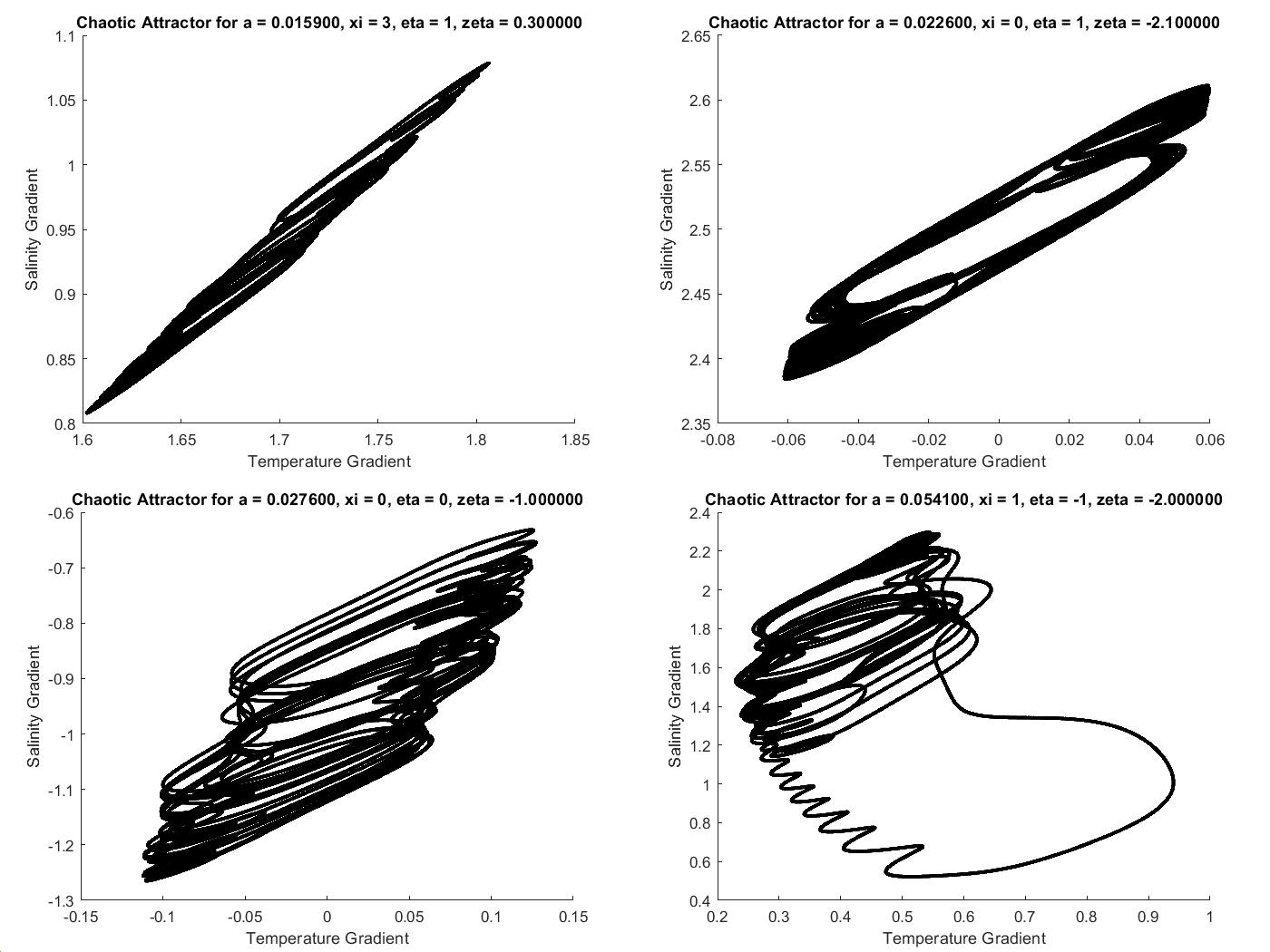
Figure 1: [Top Left, Bottom Left] Examples of single-regime chaotic attractors under Stommel parameters $(a,\xi,\eta,\zeta)$ $=$ $(0.0159,3,1,0.3)$ and $(0.0276,0,0,-1)$. [Top Right] An example of a dual-regime chaotic attractor with $(a,\xi,\eta,\zeta)$ $=$ $(0.0226,0,1,-2.1)$ [Bottom Right] An example of a single-regime chaotic attractor with $(a,\xi,\eta,\zeta)$ $=$ $(0.0541,1,-1,-2)$ that exhibits excursive behaviour, showing signs of losing stability under further forcing.

Once the forcing reaches some critical value $a_{c}$, the LFSBM undergoes a crisis, when bistability in the system collapses into monostability as a result of one of the chaotic attractors losing stability. Mehra and Ramaswamy [18] define three different types of crises for systems with multiple chaotic attractors (such as the LFSBM):

• Boundary Crises: A chaotic attractor is destroyed (typically as a result of a collision with a saddle) and is reduced to a chaotic transient that flows into another attractor.

• Interior Crises: The size of a chaotic attractor suddenly increases or decreases due to a collision with the stable manifold of an unstable periodic orbit inside its basin of attraction.

• Attractor-Merging Crises: Two or more chaotic attractors simultaneously collide with the stable manifold of an unstable periodic orbit along a shared boundary in the basin of attraction, resulting in the chaotic attractors fusing.

In their work, Mehra and Ramaswamy use the Maximal Lyapunov exponent (MLE) as a predictor of which type of crisis is likely to occur. In our chosen model (3), the combination of the Lorenz equations and a typical stable equilibrium in the Stommel model with negative Lyapunov exponents implies that the MLE of the system remains constant ($\approx 0.9057$). This means that interior and attractor-merging crises cannot occur in the LFSBM since they require significant changes in the MLE [18], but the possibility of boundary crises cannot be ruled out (we provide an example of a boundary crisis in figure 2). However there is also a fourth family of crisis defined by:

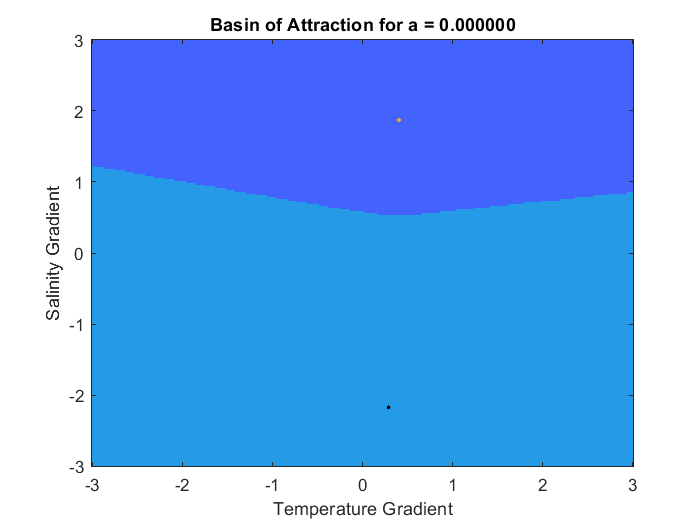
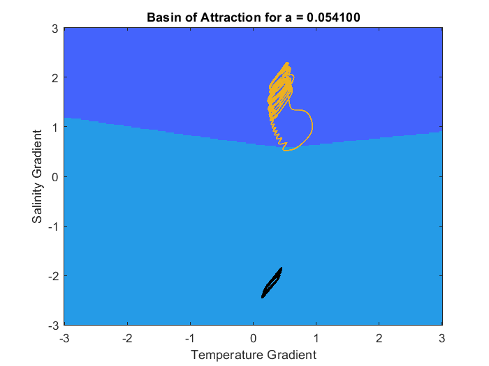
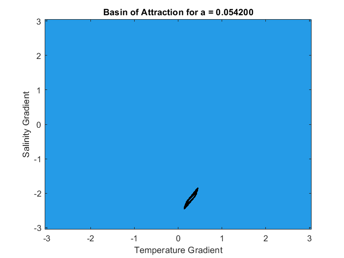
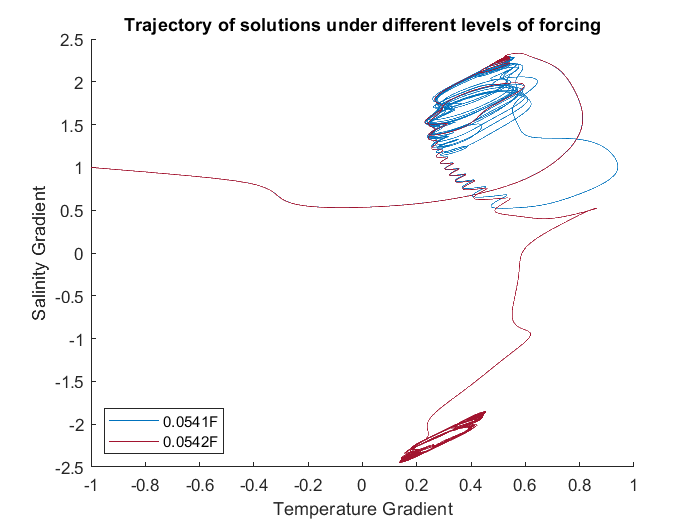
Figure 2: Basins of attraction for Stommel parameters $(\xi,\eta,\zeta)$ $=$ $(1,-1,-2)$ with Lorenz initial conditions $(x,y,z)$ $=$ $(-1,-1,-1)$; [Top Left] $a$ $=$ $0$, [Top Right] $a$ $=$ $0.0541$, and [Bottom Left] $a$ $=$ $0.0542$. Images in the top row show the thermally-driven (TH, black) and saline-driven (SA, orange) attractors. These remain stable until the boundary crisis happens in $a$ $\in$ $(0.0541,0.0542)$, at which point, the SA attractor is destroyed. [Bottom Right] shows an example trajectory with initial conditions $(T,S)$ $=$ $(-1,1)$, showing the chaotic transient that remains and the visible point of divergence between the two trajectories.

Definition 3.1 (Vanishing Basin Crisis).

Let $B_{a}(\omega_{T}(\textbf{\tt x}_{0}))$ be the basin of attraction for a chaotic attractor $\omega_{T}(\textbf{\tt x}_{0})$ at some prescribed forcing strength $a$. If, for some $a$ $=$ $a_{0}$, we have

• $B_{a_{0}+\varepsilon}(\omega_{T}(\textbf{\tt x}_{0}))$ $\subset$ $B_{a_{0}}(\omega_{T}(\textbf{\tt x}_{0}))$ (and $B_{a_{0}+\varepsilon}(\omega_{T}(\textbf{\tt x}_{0}))$ $\neq$ $\emptyset$) when $0$ $<$ $\varepsilon$ $<$ $A$ (where $A$ $=$ $a_{c}-a_{0}$ $>$ $0$), and

• $\lim_{\varepsilon\to A^{-}}|B_{a_{0}+\varepsilon}(\omega_{T}(\textbf{\tt x}_{0}))|$ $=$ $0$,

then we say that $\omega_{T}(\textbf{\tt x}_{0})$ undergoes a vanishing basin crisis, and loses its basin of attraction completely at some $a_{c}$.

We remark that for the vanishing basin crisis here, since our attention is confined to the Stommel phase plane, we only consider the values of $T$ and $S$ within the basin of attraction. We do this by fixing $(x,y,z)$ $=$ $(x_{0},y_{0},z_{0})$ at time $t$ $=$ $0$.

The main distinction between this type of crisis and the other three families, is that with the vanishing basin the crisis does not occur instantaneously. Rather, the crisis develops with an increasing forcing strength, starting from some $a_{0}$ before completely losing its stability at some $a_{c}$ $(>a_{0})$. As the forcing increases from $a_{0}$ to $a_{c}$, it can be shown that the size of the basin of attraction shrinks concomitantly. At the completion of the crisis the chaotic attractor is not destroyed. Instead, the attractor simply loses its basin of attraction and becomes a ghost attractor (a designation coined by Belykh et al. [5]). We provide an example of a vanishing basin crisis in Figure 3.

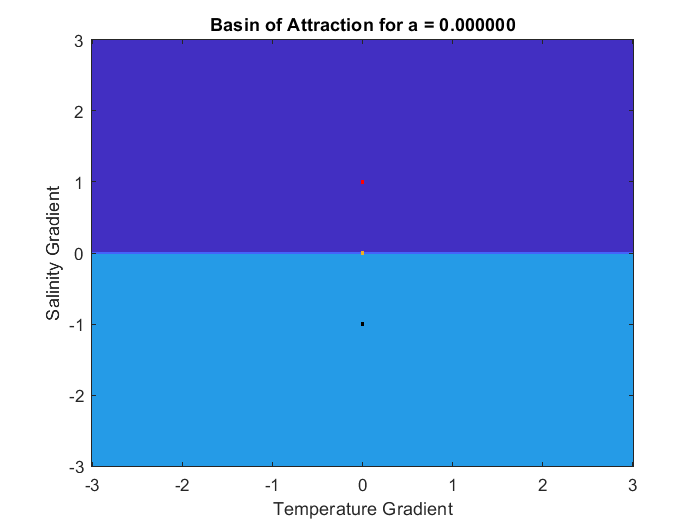
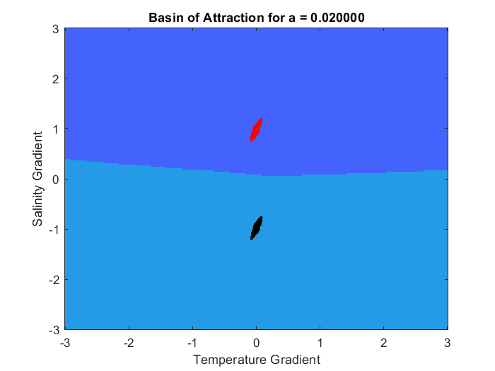
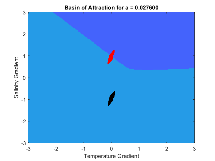
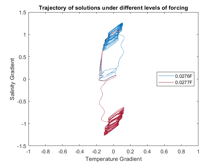
Figure 3: Basins of attraction for Stommel parameters $(\xi,\eta,\zeta)$ $=$ $(0,0,-1)$ with Lorenz initial conditions $(x,y,z)$ $=$ $(1,1,1)$; [Top Left] $a$ $=$ $0$, [Top Right] $a$ $=$ $0.02$, and [Bottom Left] $a$ $=$ $0.0276$. Images in the top row show the thermally-driven (TH, black) and saline-driven (SA, red) attractors. As forcing increases, the basin of attraction for the SA attractor starts to shrink. One such example is shown [Bottom Right] with its initial condition of $(T,S)$ $=$ $(0,1)$, losing its attraction to the SA attractor between $a$ $=$ $0.0276$ and $a$ $=$ $0.0277$.

As forcing increases past $a_{c}$, the general regime pattern that existed shortly before the crisis remains stable. It continues to develop until a second critical forcing level $a_{r}$ is attained whereupon, though the system itself remains monostable, the chaotic attractor undergoes significant structural change.

• If the system suffered a boundary crisis, then the resulting chaotic transient persists in that region of phase space before merging with the remaining chaotic attractor at forcing value $a_{r}$ (Figure 4).

• On the other hand, if the system was subject to a vanishing basin crisis, then the attractor that loses its associated basin simply vanishes from view, with solution trajectories attempting to (and failing) to locate it before entering the other attractor until the forcing reaches the value $a_{r}$.When $a$ $=$ $a_{r}$, the attractor with the disappearing basin re-appears (found by solution trajectories) and merges with the existing chaotic attractor, hence, becoming a ghost attractor (Figure 4).

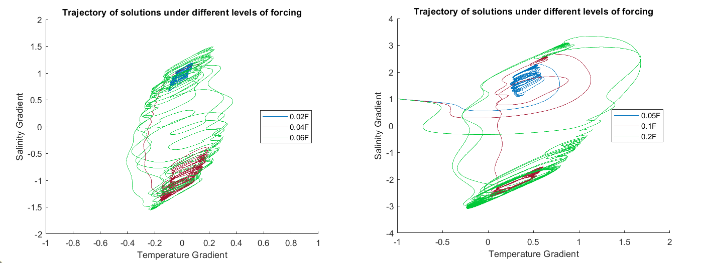
Figure 4: [Left] An example of a chaotic transient merge using Stommel parameters $(\xi,\eta,\zeta)$ $=$ $(1,-1,-2)$ with initial condition $(x,y,z,T,S)$ $=$ $(-1,-1,-1,-1,1)$. [Right] An example of a ghost attractor merge using Stommel parameters $(\xi,\eta,\zeta)$ $=$ $(0,0,-1)$ with initial condition $(x,y,z,T,S)$ $=$ $(1,1,1,0,1)$. The blue trajectory gives a chaotic attractor that loses stability after a crisis, the red trajectory depicts the remaining chaotic attractor following a crisis, and the green trajectory indicates the chaotic attractor following the ghost attractor (or chaotic) transient merge.

3.1 Chaotic Saddle Collisions

As noted previously, a boundary crisis typically occurs when a chaotic attractor collides with a chaotic saddle. In order to illustrate such an event, we examine the evolution of the chaotic attractors and saddle for the system (3). We chose a set of Stommel parameters (albeit nonphysical) which lead to a long chaotic transient after the crisis and so we selected $\xi$ $=$ $0$, $\eta$ $=$ $1$ and $\zeta$ $=$ $-2.1$. With these particular parameter values the critical forcing $a_{c}$ $\in$ $(0.0226,0.0227)$ and we explore the effect of increasing the forcing strength beyond $a_{c}$.

In order to visualise the saddle, we adopt the so-called Saddle-Straddle Algorithm [3, 19, 26]. The algorithm was originally developed in [3] as a way to detect segments which belong to the saddle. We implemented the algorithm in the manner described in [26]. In brief, the algorithm works by first selecting pairs of points which straddle the basin boundary by a predetermined length $\delta$ (we used $\delta=10^{-5}$). The points are then iterated forward under the dynamics for some chosen window and refined again to ensure that they again straddle a small segment. We then assume the midpoint of the resulting segment to be part of the chaotic saddle.

Figure 5 shows the results arising from this algorithm at increasing forcing strengths. We see that as $a$ grows, so the saddle seems to expand in width (particularly in the more central region of its “T”-shape). Additionally, the TH (thermally-driven) attractor grows in phase space and begins to approach the saddle from below. Right before the crisis ($a=0.0226$) we see the TH attractor nearly collide with the saddle. Just after the crisis ($a=0.0227$) the trajectory which shadows the previous TH attractor diverges from that attractor nearby to the apparent collision point. This creates a long chaotic transient which is not part of the surviving SA (saline-driven) attractor.

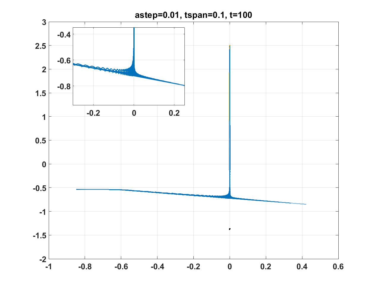
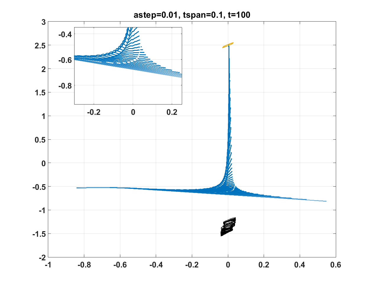
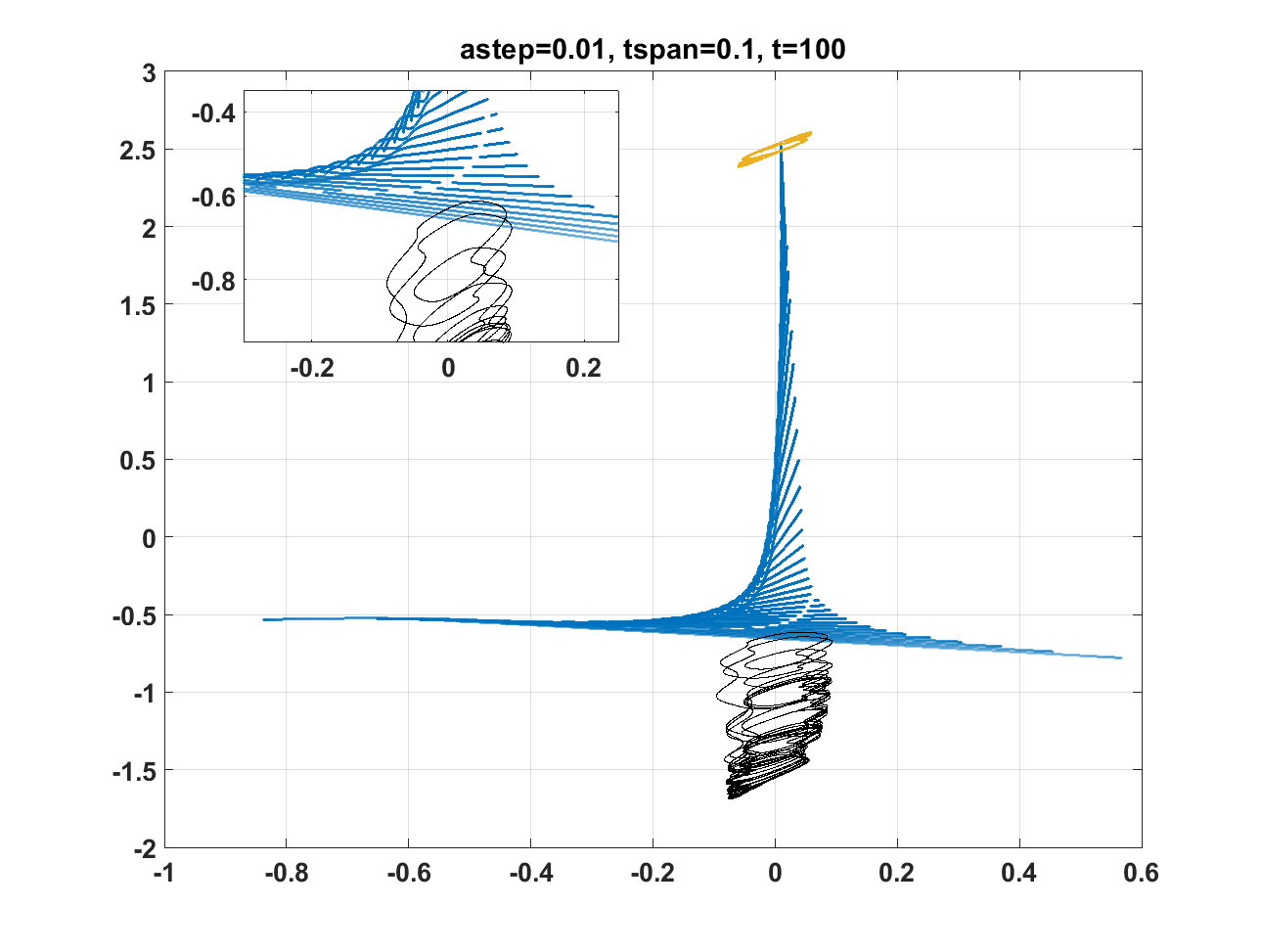
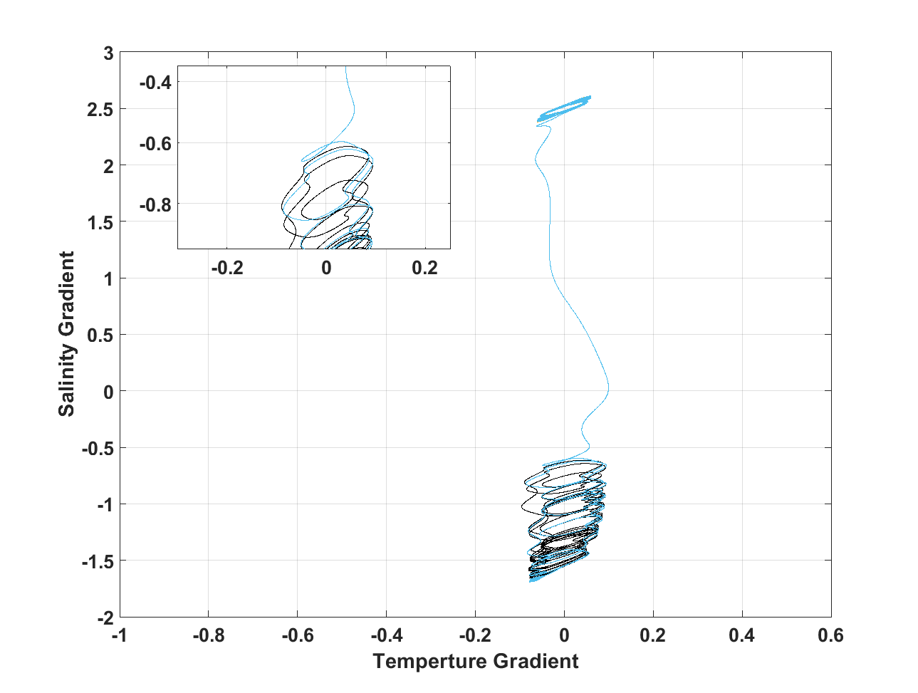
Figure 5: The evolution of the chaotic saddle at an increasing level of forcing strength: [upper left] $a$ $=$ $0.001$, [upper right] $a$ $=$ $0.0113$ and [lower left] $a$ $=$ $0.0226$. In these three frames the dark blue depicts the chaotic saddle, black the TH (thermally-driven) attractor, and gold the SA (saline-driven) attractor. [Lower right] The trajectory for the same initial conditions is plotted for $a$ $=$ $0.0226$ (black) and $a$ $=$ $0.0227$ (turquoise).

The behaviour depicted in Figure 5 is very interesting when viewed from a finite-time standpoint. While the asymptotic behaviour after the crisis is convergence to the SA attractor, the system spends a long period of time elsewhere in phase space tracing the previously existing TH attractor. If this process were analysed in isolation, this might seem to be a potentially reversible transition between the TH and SA states,whereas in actuality the crisis has already occurred and the system is destined to eventually converge to the SA attractor. Similar behaviour has previously been seen in quasi-periodically forced delay models [21, 22] and in systems with delayed Hopf bifurcations (see e.g. [13] and references therein). In both of the aforementioned cases, the system undergoes a bifurcation in which the stability of one attractor is lost, but if initial conditions are sufficiently close to that attractor, then the trajectory can remain near it for an extended period of time before converging to the true attractor. Such behaviour is important to understand when considering reversible and irreversible transitions or regime shifts.

4 Finite-time Analysis

We begin with the aim of seeing how the FTLEs of the system change over the course of a given solution trajectory for a given set of initial conditions and parameters. In order to do this, we require the use of various numerical methods (see Appendix A for details). From this, we derive five different FTLEs at any given point along the trajectory, three of which are associated with the Lorenz attractor forcing, and the other two with the SBM response. For our finite-time analysis, we arbitrarily set the step size for our FTLEs (and the ODE solver by extension) to be $\Delta t$ $=$ $\frac{1}{400}$, and chose to calculate across the range $t$ $\in$ $[0,100]$, giving us 40,000 time steps in total. Any time step can be implemented and the detailed quantitative properties of the chaotic signal induced will be sensitive to time-step as will the change in the level of forcing required to induce a crisis depending on the parameters. We also remark at this point that the length of the FTLE window we select for the study will give different results in terms of FTLE behaviour; while smaller FTLE windows tend to give more volatile results, longer windows typically lead to much smoother outcomes. While we will discuss other FTLE windows at appropriate stages we set our default FTLE window to 400 time steps (i.e. of length 1). The five FTLEs we derive for the LFSBM are referred to in their typical order from highest to lowest: the unstable Lorenz FTLE, the neutral Lorenz FTLE, the first Stommel FTLE, the second Stommel FTLE and the stable Lorenz FTLE.

We first consider the Stommel FTLEs in the unforced case ($a$ $=$ $0$). For a bistable system with two stable equilibria in differing regions (one in the TH region, the other in the SA region of the phase plane) the behaviour of these FTLEs will mostly depend on the nature of the equilibrium in the region of the phase plane given by performing Hartmann linearisation on equation (1). If the equilibrium in the region is a stable node, then the Stommel FTLEs will converge towards the two eigenvalues of the stable node and then remain without major change (and does not vary with different FTLE window lengths). We refer to this natural behaviour of the Stommel FTLEs as distinct separation. If the equilibrium in the region is considered a stable focus, however, then the Stommel FTLEs will oscillate between two different values. This oscillation will be centred around the value of the real part of the eigenvalues, and with an amplitude that is dependent on the length of the FTLE window. A longer FTLE window will see the amplitude trend towards zero, while a shorter FTLE window will see the amplitude approaches the imaginary part of the eigenvalues (Figure 6). We refer to this natural behaviour of the Stommel FTLEs as a rapid oscillation. We showcase the two natural behaviours in Figure 7.

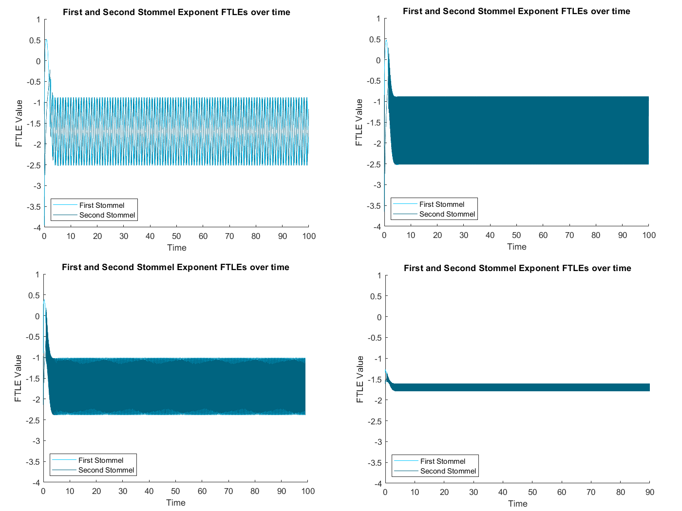
Figure 6: The evolution of the Stommel FTLEs over the trajectory corresponding to parameter choices $(\xi,\eta,\zeta)$ $=$ $(1,-1,-2)$ and initial condition $(x,y,z,T,S)$ $=$ $(-1,-1,-1,-1,1)$ and with no forcing. [Top-Left] A window size of 0.01 (4 steps), [Top-Right] A window size of 0.1 (40 steps), [Bottom-Left] A window size of 1 (400 steps), [Bottom-Right] A window size of 10 (4,000 steps).

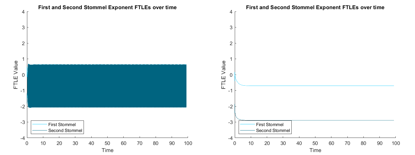
Figure 7: [Left] An example of rapid oscillation behaviour in the Stommel FTLEs under no forcing. [Right] An example of distinct separation behaviour in the Stommel FTLEs under no forcing.

As forcing is introduced to the model, the Stommel FTLEs start to behave differently depending on the strength of the forcing. With the aforementioned window choice, the Stommel FTLEs start to exhibit spikes in their values at certain points along the trajectory (these are smoothed out in the larger window choices, see Figure 8), while the general values and bounds start to vary over time (Figure 9). If the trajectory of a solution crosses regions (e.g. from TH to SA, temporarily or otherwise), the FTLEs will exhibit the behaviour associated with the other region. This general behaviour persists as the forcing strengthens until it nears the crisis point. Around this stage, we begin to notice some more significant differences in the behaviour of the Stommel FTLEs (though this will vary from case to case). One such notable change is signs of FTLE alignment, particularly between the first Stommel and neutral Lorenz FTLEs. An example of this can be seen in Figure 8 (Top Left).

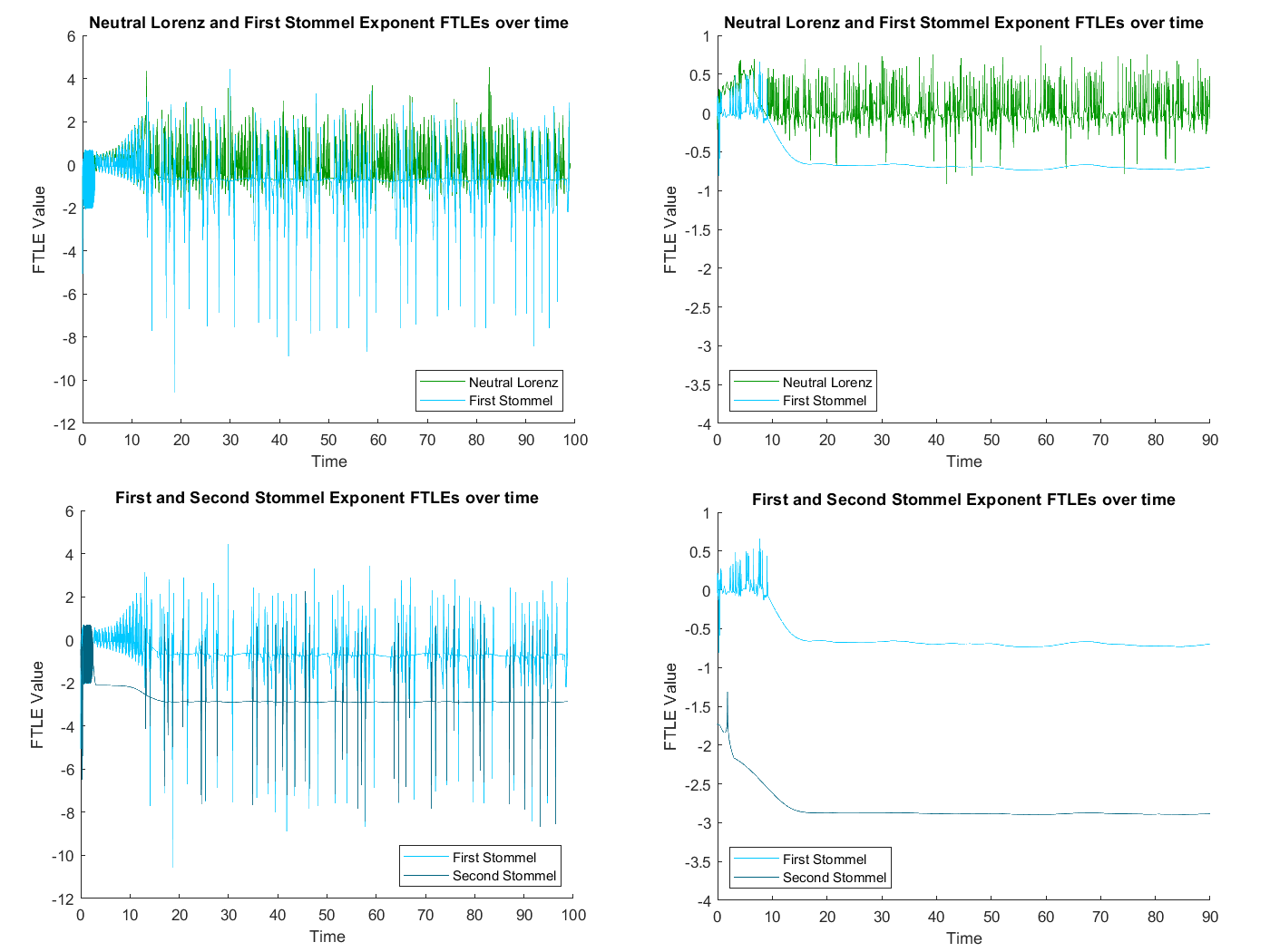
Figure 8: The FTLEs along the trajectory given Stommel parameters $(\xi,\eta,\zeta)$ $=$ $(3,1,0.3)$, initial condition $(x,y,z,T,S)$ $=$ $(1,1,1,2.8,2.8)$ and a forcing of strength $a$ $=$ $0.0160$. [Left] A window length of 1 (400 steps), and [Right] a window length of 10 (4,000 steps). [Top] A comparison of the neutral Lorenz and first Stommel FTLEs, while [Bottom] compares the two Stommel FTLEs. The loss of useful information with an increasing the window length is noticeable.

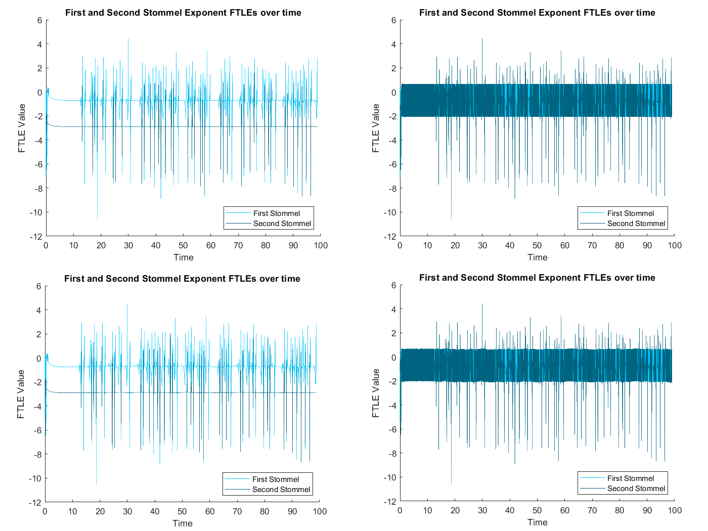
Figure 9: Some distinct separation [Left, $(T,S)$ $=$ $(1.4,1.4)$] and rapid oscillation [Right, $(T,S)$ $=$ $(2.8,2.8)$] behaviours under forcing strengths $a$ $=$ $0.001$ [Top] and $a$ $=$ $0.01$ [Bottom] for Stommel parameters $(\xi,\eta,\zeta)$ $=$ $(3,1,0.3)$ and Lorenz initial conditions $(x,y,z)$ $=$ $(1,1,1)$. The differences between the two levels in forcing arise owing to subtle variations along the trajectory.

To assess the alignment between the neutral Lorenz and first Stommel FTLEs, we used a simple absolute distance metric, which is defined as:

(10) $$d(x_{1},x_{2}):=|x_{1}-x_{2}|$$

for some scalars $x_{1}$ and $x_{2}$ (representing the two FTLEs at a point in time). We measure the gap between the two FTLEs at a given instant in time, taking lower distances to be indicative of a stronger alignment. Using this metric, we found that just before and just after a crisis, this alignment is at its strongest when the trajectory is at a critical juncture such that only a slight increase in the forcing strength will be enough to cause convergence to switch to other attractor (Figure 10). This strong alignment is more evident in cases where the attractor that loses stability under forcing resides in the SA region, but is sill present in the cases where the trajectory initially enters the TH attractor (Figure 11). However, the general alignment strength between the neutral Lorenz and first Stommel FTLEs across the entirety of a trajectory before and after a crisis is dependent on the system and initial conditions. In some cases there is a clear strengthening of the alignment, while others demonstrate a general weakening of the alignment, particularly in those cases when the remaining stable attractor is of the dual-regime type. (The example in Figure 11 is one where the stable attractor is a dual-regime attractor.) In general, however, more useful measures for alignment strength already exist in the use of Lyapunov vectors, which not only help characterise the dynamics of a system [12], but strong levels of alignment can be used to predict chaotic transitions (e.g. [4], [23]). Future research in the area would endeavour to identify some measure that could better characterise this alignment between the two FTLEs.

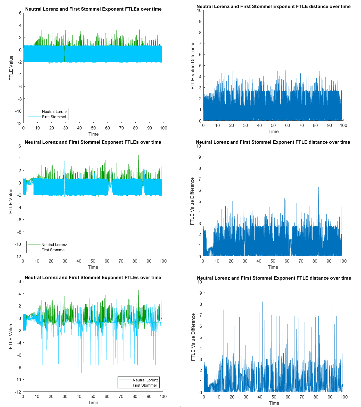
Figure 10: The neutral Lorenz and first Stommel FTLEs for parameters $(\xi,\eta,\zeta)$ $=$ $(3,1,0.3)$ and initial conditions $(x,y,z,T,S)$ $=$ $(1,1,1,2.8,2.8)$ when [Top] $a$ $=$ $0.01$, [Centre] $a$ $=$ $0.0159$, and [Bottom] $a$ $=$ $0.0160$. The results in the left-hand column show the values across the trajectory while the right-hand column demonstrates the distance between the two FTLEs across the trajectory. We see that as we approach the crisis there is a more visible alignment between the two FTLEs at certain points along the trajectory.

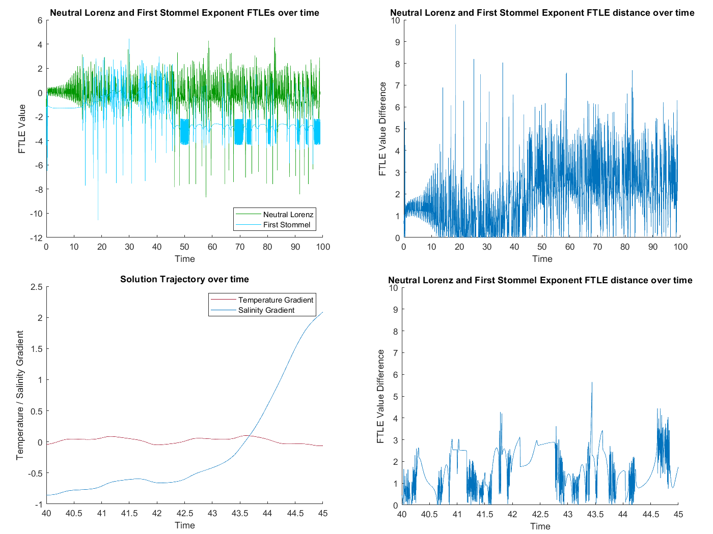
Figure 11: Results for parameters $(\xi,\eta,\zeta)$ $=$ $(0,1,-2.1)$ and initial condition $(x,y,z,T,S)$ $=$ $(1,1,1,0,-2)$ when $a$ $=$ $0.0227$ (This forcing is sufficiently strong that the system undergoes a boundary crisis prior to $t$ $=$ $100$): [Top Left] The neutral Lorenz and first Stommel FTLEs along the trajectory and [Top Right] the value difference between the two FTLEs along the trajectory. The period of alignment for this and any other TH to SA attractor case is not particularly obvious, but if we zoom to around the point of transition from TH to SA [Bottom Left] and observe the value difference in this interval of $t$ $\in$ $[40,45]$, we see a number of points in this interval where the two FTLEs are visibly close for long enough, especially around the point of transition.

Another notable change that happens to FTLEs as the forcing strength increases is that we notice instances in which the neutral Lorenz and first Stommel FTLEs interchange modes (see Figure 12 for an example of how the neutral Lorenz value is affected by the forcing strength). However, it is not evident as to whether this behaviour is a property inherent within these forced systems or is actually a side-effect of the algorithm used to calculate the FTLEs (a backwards QR method with Gram-Schmidt orthogonalisation). The algorithm works nicely when the FTLEs are reasonably well spaced, but tends to lose accuracy as the FTLEs approach each other. (This is a plausible explanation for the mode-swaps that we occasionally see for these trajectories.) This can be further affected by the particular algorithm used in calculating a new set of FTLEs at every time step. Further research in the area would test alternative algorithms for calculating FTLEs; this would shed light on the question as to whether the algorithm is directly contributing to the phenomenon of mode swapping.

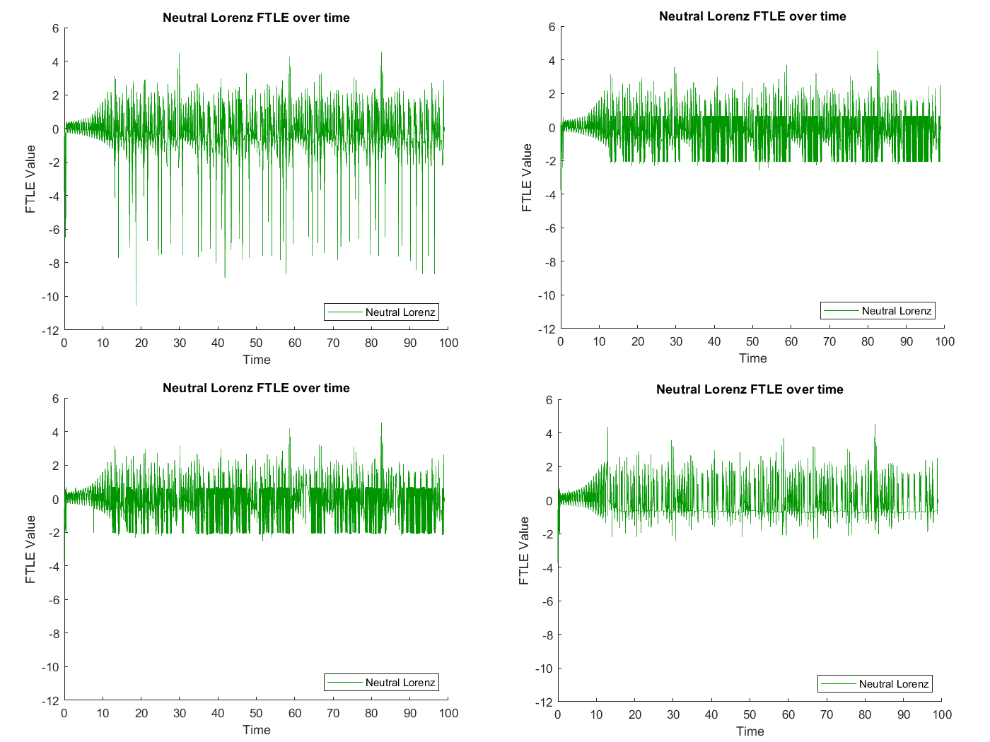
Figure 12: Given Stommel parameters $(\xi,\eta,\zeta)$ $=$ $(3,1,0.3)$ and initial condition $(x,y,z,T,S)$ $=$ $(1,1,1,2.8,2.8)$, The neutral Lorenz FTLE along the trajectory for: [Top Left] $a$ $=$ $0$, [Top Right] $a$ $=$ $0.0001$, [Bottom Left] $a$ $=$ $0.0159$, and [Bottom Right] $a$ $=$ $0.0160$. We see as forcing is introduced that the neutral Lorenz FTLE is clearly influenced by the Stommel FTLEs and takes on a similar mode to what those FTLEs would do under the given level of forcing. This gives us the “mode-swapping” behaviour.

One key issue relates to the question as to whether there is a reliable predictor as to which chaotic attractor will be the one that loses stability as the forcing strength increases. We have been unable to find a definitive answer, but some possible predictors can be ruled out. In the course of our work, we looked at both the sum of Lyapunov exponents and the Kaplan-Yorke dimension [14] as possible predictors of a crisis. For the first of these, we conjectured that of the two chaotic attractors in a bistable solution, the attractor with the greater sum of Lyapunov exponents (under no forcing) would lose stability under imposed forcing. However, if we study equation (3) with $(\mu,\rho,\beta,\xi,\eta,\zeta)$ $=$ $(10,28,\frac{8}{3},3,1.2,0.3)$, we find that

• Sum of exponents (TH attractor): 0.905650 - 0.000462 - 14.573199 - 0.212948 - 2.587471 = -16.46843 (No Forcing)

• Sum of exponents (SA attractor): 0.905650 - 0.000462 - 14.573199 - 0.844421 - 0.850531 = -15.362963 (No Forcing)

As we would expect, it is the TH attractor that has the lower sum of Lyapunov exponents, but under forcing, the TH attractor is the one that collapses (Figure 13). Hence, unfortunately, we cannot rely on using the sum of Lyapunov exponents to predict a collapse.

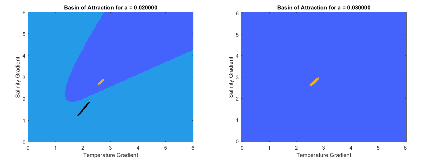
Figure 13: A counterexample to the idea of using Lyapunov exponent sums to predict the identity of a crisis. [Left] The basin of attraction when $a$ $=$ $0.02$. [Right] The basin of attraction when $a$ $=$ $0.03$. Eventually, the TH attractor (black) undergoes a boundary crisis and its transient will flush into the SA attractor (orange), despite having the lower sum of exponents.

If we turn to the Kaplan-Yorke dimension, we speculated that of the two chaotic attractors in a bistable solution, the one with the higher Kaplan-Yorke dimension (in the absence of forcing) would lose stability when forced. We calculated the Kaplan-Yorke dimension using:

(11) $$D_{L}:=j+\frac{\lambda_{1}+\lambda_{2}+...+\lambda_{j}}{|\lambda_{j+1}|},$$

for a given Lyapunov spectrum $\{\lambda_{1},\lambda_{2},...,\lambda_{n}\}$ ordered so that $\lambda_{1}$ $\geq$ $\lambda_{2}$ $\geq$ $...$ $\geq$ $\lambda_{n}$, and where $j$ is the largest number such that $\lambda_{1}+\lambda_{2}+...+\lambda_{j}$ $>$ 0. However, if we select $(\mu,\rho,\beta,\xi,\eta,\zeta)$ $=$ $(10,28,\frac{8}{3},3.01,6,2)$ with any non-equilibrium initial condition, then we obtain a case where it is the attractor with the lower Kaplan-Yorke dimension that actually loses stability under forcing. This gives us two attractors, the SA attractor at $(T,S)=(2.351467,2.631519)$, and the TH attractor at $(T,S)=(2.998013,2.994014)$. These attractors have the following Lyapunov exponents:

• LEs (TH attractor): 0.90565, -0.000462, -1.505546, -1.506779, -14.573199,

• LEs (SA attractor): 0.90565, -0.000462, -0.258749, -3.582122, -14.573199,

which yields Kaplan-Yorke dimensions of 2.601236 (TH) and 3.180463 (SA) respectively. When forcing increases, we find that it is the TH attractor which loses stability (Figure 14). This contradicts our supposition that the attractor with the lower Kaplan-Yorke dimension remains stable under forcing. Thus both the sum of Lypunov exponents and the Kaplan-Yorke dimension cannot be relied as accurate forecasters as to which unforced attractor will evenutally lose stability. It would be of interest to identify some other characteristic which might be of more help in this regard.

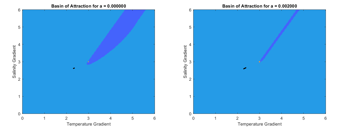
Figure 14: The counterexample for the Kaplan-Yorke dimension. [Left] The basin of attraction under no forcing. [Right] The basin of attraction under a forcing strength of $a$ $=$ $0.002$. The TH attractor (orange) is clearly undergoing a vanishing basin crisis as forcing increases, losing its stability at roughly $a$ $\approx$ $0.0024$.

5 More general considerations

We next ask as to the wider applicability of some of our findings. We do this by looking at the properties of crises and finite-time analysis as they relate to the SBM forced now, not by the L63 model, but by other “strange” attractors. Several candidate models were considered, but after extensive testing, we restrict our comments to the Rössler, the Four-Wing and the Halvorsen attractor. In particular, for the Rössler-forced model, we took

(12) $$\begin{array}[]{lcl}\dot{x}(t)&=&-(y+z),\\ \dot{y}(t)&=&x+dy,\\ \dot{z}(t)&=&c+z(x-d),\\ \dot{T}(t)&=&\xi+ax-T(1+|T-S|),\\ \dot{S}(t)&=&\eta+ax-S(\zeta+|T-S|),\end{array}$$

in which the parameters $(b,c,d)$ $=$ $(0.2,0.2,5.7)$. This combination is known to generate a chaotic signal [15]. For the Four-Wing-forced model, we supposed

(13) $$\begin{array}[]{lcl}\dot{x}(t)&=&bx+yz,\\ \dot{y}(t)&=&cx+dy-xz,\\ \dot{z}(t)&=&-(z+xy),\\ \dot{T}(t)&=&\xi+ax-T(1+|T-S|),\\ \dot{S}(t)&=&\eta+ax-S(\zeta+|T-S|),\end{array}$$

with $(b,c,d)$ $=$ $(0.2,0.02,-0.4)$, see [27]. Lastly, for the Halvorsen-forced model:

(14) $$\begin{array}[]{lcl}\dot{x}(t)&=&-(bx+4y+4z+y^{2}),\\ \dot{y}(t)&=&-(by+4z+4x+z^{2}),\\ \dot{z}(t)&=&-(bz+4x+4y+x^{2}),\\ \dot{T}(t)&=&\xi+ax-T(1+|T-S|),\\ \dot{S}(t)&=&\eta+ax-S(\zeta+|T-S|),\end{array}$$

where $b$ $=$ $1.27$, [25].

We subjected these systems to the same procedures as applied to the LFSBM. We found that vanishing basin crises (3.1) can be replicated in the Halvorsen-forced model (14) with similar sets of Stommel parameters as the LFSBM. Other strange attractors tested did not seem to undergo such a crisis. We note that when $(\xi,\eta,\zeta)$ $=$ $(3,1,0.3)$ the Rössler-forced model (12) has an SA attractor whose basin decreases with forcing, but which undergoes a regular boundary crisis when $a\approx 0.0229$ (Figure 15), unlike the Lorenz-forced and Halvorsen-forced models. The underlying reason why the Lorenz and Halvorsen models can give solutions that exhibit vanishing basin crises while the Rössler and Four-Wing models is not yet known. This is a possible topic for future research.

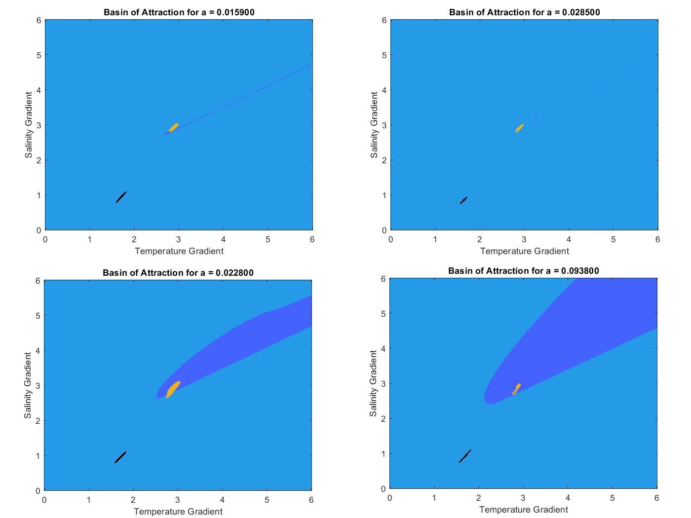
Figure 15: Basin of attractions for Stommel parameters $(\xi,\eta,\zeta)$ $=$ $(3,1,0.3)$ at crisis levels of forcing for the following: [Top-Left] The Lorenz-forced model with initial condition $(x,y,z)$ $=$ $(1,1,1)$ and $a=0.0159$, [Top-Right] The Halvorsen-forced model with initial condition $(x,y,z)$ $=$ $(1,1.1,1.2)$ and $a=0.0285$, [Bottom-Left] The Rössler-forced model with initial condition $(x,y,z)$ $=$ $(1,1,1)$ and $a=0.0228$, [Bottom-Right] The Four-wing-forced model with initial condition $(x,y,z)$ $=$ $(1,1,1)$ and $a=0.0938$. This shows the contrast between the vanishing basin crises for the Lorenz- and Halvorsen-forced models and the boundary crises for the Rössler- and Four-wing-forced models in the significantly smaller (almost invisible in cases) basin of attractions for the attractors in question.

Our findings using other strange attractors also suggest a possible link between the number of regimes in a chaotic attractor and whether or not we can obtain persisting chaotic attractors that merge with chaotic transients under significant levels of forcing. We found that the behaviour of chaotic attractors that combine with chaotic transients (from a boundary crisis) in the Lorenz-forced model, a two-regime attractor, could be reproduced in the Four-wing-forced model, which is a four-regime attractor (Figure 16). However, we could find no analogous results for either the Rössler or Halvorsen examples, both of which are single-regime attractors. Future research in the matter might either validate or disprove such a conjecture with regards to resulting chaotic transients (and ghost attractors in the case of a vanishing basin crisis).

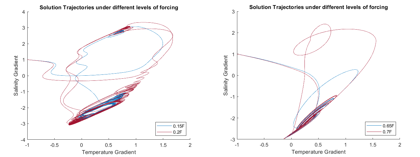
Figure 16: [Left] The Lorenz-forced model with forcing levels $a=0.15$ and $a=0.2$. [Right] The Four-wing-forced model with $a=0.65$ and $a=0.7$. In both cases $(\xi,\eta,\zeta)$ $=$ $(1,-1,-2)$ and the initial conditions chosen are $(x,y,z,T,S)$ $=$ $(-1,-1,-1,-1,1)$. These results demonstrate how the chaotic attractor develops eventually merges with a resulting chaotic transient after a crisis.

In the Lorenz-forced model we found that the neutral Lorenz and first Stommel exponents aligned strongly at forcing levels around crises near the point where a trajectory is at its most sensitive (to ending up in either chaotic attractor). Finite-time analysis of the other forced models show that this alignment of the first Stommel FTLE and the equivalent neutral FTLE is also present in the other forced models (Figure 17) according to the absolute distance metric defined in equation (10). Instances of “mode-swapping” after a given crisis between the Stommel FTLEs and the strange attractor FTLEs also appear when the Stommel model is forced by other strange attractors.

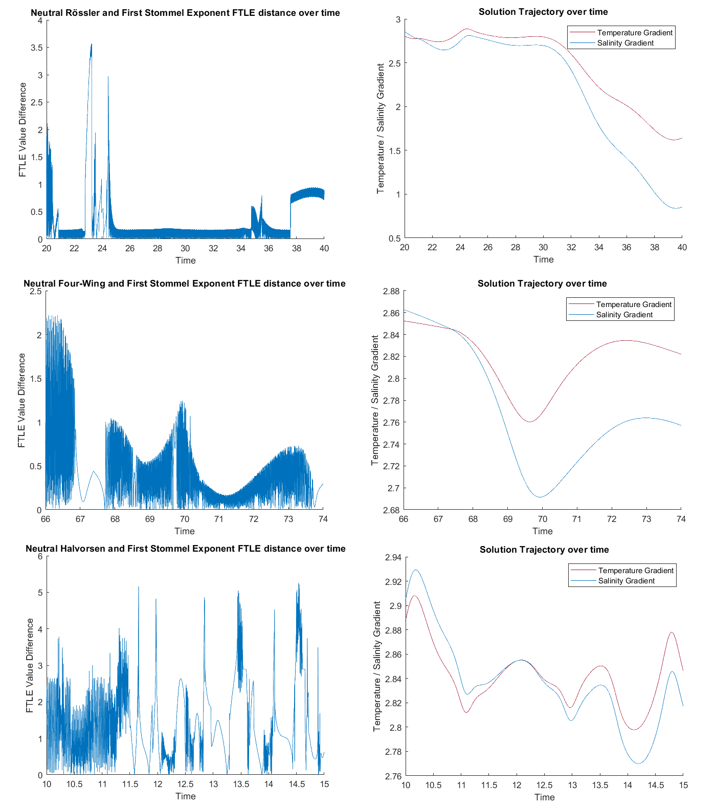
Figure 17: Results of simulations with parameters $(\xi,\eta,\zeta)$ $=$ $(3,1,0.3)$ and initial conditions $(x,y,z,T,S)$ $=$ $(1,1,1,2.8,2.8)$. Here we have conducted finite-time analysis using the Rössler-forced model [Top, $a$ $=$ $0.0229$], the Four-wing-forced model [Centre, $a$ $=$ $0.0939$], and the Halvorsen-forced model [Bottom, $a$ $=$ $0.0286$], and analyse around the time period where the solution trajectory permanently transitions from the SA region to the TH region [Right]. We note that the distance between the first Stommel and neutral attractor FTLEs [Left] during this transition is at its strongest either at the TH/SA transition (Halvorsen) or at points along the transition to the TH attractor (Rössler and Four-Wing to a lesser extent).

6 Conclusion

The Lorenz-Forced Stommel Box Model LFSBM, as defined by equation (3), is a recent hybrid model introduced by Ashwin and Newman in their study on measures for pullback attractors and tipping point probabilities [2]. We have explored solutions to the autonomous forced model in parameter regions that are bistable under no forcing, and have paid particular attention to forcing strengths around levels that induce a crisis which reduces the system to monostability. We have found two different types of crises in the model: a vanishing basin crisis that results in the basin of attraction for a chaotic attractor deplete over time (and ultimately become a ghost attractor), and a boundary crisis in which a chaotic attractor is destroyed following a collision with a chaotic saddle or other feature of the system. We also find that further increases to the forcing strength can mean that the surviving chaotic attractor merges with either a chaotic transient or a ghost attractor depending on the type of crisis to hand.

Performing finite-time analysis on the LFSBM reveals that with no forcing, the Stommel FTLEs will either oscillate between two specific values or converge to particular values depending on the nature of the attractor it enters (in both cases, this is dependent on the Stommel eigenvalues of the attractor). With forcing present, these Stommel FTLEs start to behave a little more like Lorenz FTLEs, potentially mode-swapping with them on occasion, and near crisis levels we found that the neutral Lorenz and first Stommel FTLEs start to align around the point where a solution trajectory is at its most sensitive to transitioning to one or the other of the chaotic attractors.

Our experiments in which we forced the Stommel model with other strange attractors enabled us to draw some conclusions as to the possible generality of the earlier findings. We could replicate the strong alignment between the first Stommel and the neutral strange attractor FTLEs in the most sensitive areas, while the observations regarding attractors merging with transients and the vanishing of basin crises do depend on the identity of the strange attractor in question. We conjecture that whether an attractor merges with the chaotic transient of a destroyed attractor (or a ghost attractor) depends on the regime count of the strange attractor used (where two or more regimes in the strange attractor are a requirement), while a possible explanation for the vanishing basin crisis that are seen in the Lorenz-forced and Halvorsen-forced model (14) is currently not apparent.

Possible avenues for future research in the area include the use of Lyapunov vectors to better understand FTLE alignment just prior or subsequent to a crisis. It would be helpful to ascertain whether mode-swapping is an artefact of the use of the backwards QR algorithm with Gram-Schmidt orthogonalisation to calculate FTLEs. A further open question concerns the link between the regime count of a strange attractor and whether a stable chaotic attractor merges with a chaotic transient or ghost attractor.

Appendix A Numerical Methods

In order to analyse crises in the LFSBM (equation (3)), we needed to resort to numerical methods. In this appendix, we outline the techniques we employed to generate the results described in the body of the paper. All calculations were performed using MATLAB R2022a and we used standard ODE solvers to compute the solution trajectories, to calculate Lyapunov exponents and their finite-time equivalents along a trajectory, and to estimate the basin of attraction for a given (chaotic) attractor.

A.1 The ODE solver

The basic building block we used to obtain our results is an appropriate ODE solver. In this study, we emplioyed the standard fourth order Runge-Kutta scheme, which can be described by the following for a given system of differential equations:

(15) $$\begin{array}[]{lcl}K_{j}^{(1)}&=&F(t_{j},Y_{j}),\\ K_{j}^{(2)}&=&F(t_{j}+\frac{1}{2}{\Delta t},Y_{j}+\frac{1}{2}{\Delta t}K_{j}^{(1)}),\\ K_{j}^{(3)}&=&F(t_{j}+\frac{1}{2}{\Delta t},Y_{j}+\frac{1}{2}{\Delta t}K_{j}^{(2)}),\\ K_{j}^{(4)}&=&F(t_{j}+\Delta t,Y_{j}+\Delta tK_{j}^{(3)}),\\ Y_{j+1}&=&Y_{j}+\frac{1}{6}{\Delta t}[K_{j}^{(1)}+2K_{j}^{(2)}+2K_{j}^{(3)}+K_{j}^{(4)}],\\ t_{j+1}&=&t_{j}+\Delta t,\end{array}$$

where $h$ is the size of the time step, $F$ represents the system of differential equations, $t_{j}$ is the time at the $j^{th}$ step, $Y_{j}$ is the solution trajectory at the $j^{th}$ step, and $K_{j}^{(i)},i\in\{1,2,3,4\}$ are the intermediate evaluations for the method. In this study, we chose to hold $\Delta t$ constant, giving us equivalent spacing throughout the lifespan of the trajectory. This is important for the calculation of FTLEs, as it allows us to use constant size windows and by extension, a constant number of data points in the FTLE calculation. In addition to the FTLE calculation, the ODE solver underpins everything else we do in this study.

A.2 Lyapunov Exponents

The Lyapunov exponents for a given trajectory were calculated using the backwards QR method coupled to Gram-Schmidt orthogonalisation.

We began with the specified system of differential equations, an initial condition, the time interval over which we wished to calculate our exponents ($t$ $\in$ [$T_{0}$, $T_{m}$]), the time-step $\Delta t$, the tolerance value $\varepsilon$, and a parameter $r$. This latter quantity was used as a refresh rate to inform us as to how many steps should be taken before we reset the $Q$ and $R$ matrices through the Gram-Schmidt process (we took $r$ $=$ $1$ for this study). We then computed the solution trajectory over the given time interval using $N$ $=$ $(T_{m}-T_{0})/\Delta t$ steps and starting at time $T_{0}$. At this point in space, we computed the Jacobian $J$, evaluated the exponential matrix $A$ $=$ $e^{J}$ and set the matrix $Q$ to be the identity matrix before entering the calculation loop.

The main calculation loop was done through the use of a backwards QR algorithm, see, for example, [9]. We initiated the calculation loop by putting $Q$ $=$ $AQ$ and whenever the $Q$ and $R$ matrices needed to be reset we performed Gram-Schmidt orthogonalisation using $Q$ and returning $Q$ and $R$. In our algorithm, we refreshed $Q$ and $R$ after every step. We then took the diagonal elements of $R$ and then added the logarithm of each value to our Lyapunov spectrum. Next, we then prepared for the next iteration of the loop by progressing to the following step on the trajectory, taking the Jacobian $J$ at that point, and then letting $A$ $=$ $e^{J}$. Once we had completed our calculation loop, we divided each element by the total number of time steps $N$, and returned the Lyapunov spectrum. In short, we defined $Q_{i}$ and $R_{i}$ iteratively by the QR decomposition of $A_{i}Q_{i-1}$ such that

(16) $$Q_{i}R_{i}=A_{i}Q_{i-1},$$

and stored each $R_{i}$, calculating each Lyapunov exponent via

(17) $$\lambda_{j}=\frac{1}{N}\sum_{1=1}^{N}\ln{R_{i,jj}},$$

where $j$ represents the $j^{th}$ row of the spectrum vector. For this study, we used the Gram-Schmidt Orthogonalisation code available online from web.mit.edu [20].

A.3 Basins of Attraction

After computing the Lyapunov exponent over the time interval [$T_{0}$, $T_{m}$] (noting, in passing, that this becomes a FTLE as a result of being a finite interval in contrast to the standard exponent that corresponds to the limit as $t$ $\rightarrow$ $\infty$), we can used it for two applications. The first, and major application, is in the calculation of the basin diagrams; a graphical output of the basin of attraction for given chaotic attractors. This method, as piloted by Armiyoon and Wu [1], takes advantage of an invariance property that Lyapunov exponents have on a given chaotic attractor to efficiently compute the numerical basin of attraction for some given chaotic attractors. While Armiyoon and Wu [1] used Monte Carlo techniques to mitigate the run time for finding basins of attraction, we instead optimise by limiting our range to the most relevant sections of the Stommel phase plane (either $T$, $S$ $\in$ [$-3$, $3$], or $T$, $S$ $\in$ [$0$, $6$]), calculating over the finite interval, and taking advantage of the fact that given our ODE solver (15), solution trajectories will inevitably converge in finite time, guaranteeing similar Lyapunov exponents to confine the range of our calculation to a very small interval.

After accounting for some basic initial conditions, we started by specifying the region in which we calculate the basin of attraction. The grid was discretised through the use of a single variable for the step parameter. A smaller parameter gives a higher resolution, but the price to be paid is a commensurate increase in the computational time. Each initial condition was assigned a colour, was decided by taking the resulting Lyapunov spectrum and comparing them to the current list of spectra. If the Lyapunov spectrum was unique, then we considered it to be a new chaotic attractor, recorded the trajectory and proceeded. Otherwise, we grouped it in with the appropriate existing spectrum and assigned it the corresponding colour. We expected a maximum of three attractors in any given basin, so if we found more than three or there were some that did not converge, we used a default colour (yellow) to indicate that the calculation has failed. Owing to the invariance property of Lyapunov exponents, we could minimise the time spent calculating the spectrum for each initial condition by restricting the computation to the latter portion of the trajectory without significant difference in the basin of attraction. Once all the initial conditions had been considered, we then output the basin of attraction and for each attractor, we recalculated the Lyapunov spectrum for accuracy and added the chaotic attractor to the basin diagram.

This algorithm is not without its faults, however. One of the main issues arose when two attractors in different parts of the phase plane possessed identical Lyapunov exponents; an example of this occurs in equation ((3) when $\xi,\eta,a$ $=$ $0$ and $\zeta$ $<$ $0$. From a behavioural analysis, we know that equilibria will be present at $(T,S)$ $=$ $(0,\pm\zeta)$, so we could use this knowledge to hard-code one of the equilibria in this instance, and call on our knowledge of the stable manifold of the saddle at $(T,S)$ $=$ $(0,0)$ to use a different colour for the $S$ $>$ $0$ region.

A.4 FTLEs

The other major application of the Lyapunov exponent is to calculate the FTLEs along a given solution trajectory. In order to do this, we needed to take a windowed approach. The algorithm we used takes the same parameters were used to compute a regular Lyapunov exponent alongside an extra variable $I$ to denote the length of each time interval (in the default MATLAB time unit of seconds). Given the interval over which we wished to calculate the trajectory $T_{m}$, the length of a given time step $\Delta t$, and the interval for an individual FTLE calculation $I$, we then began the computation by calculating the FTLEs in the interval $[T_{0},T_{0}+I]$. We then incremented the window by $\Delta t$ and then found the FTLEs over the interval $[T_{0}+\Delta t,T_{0}+\Delta t+I]$. We continued to increment by $\Delta t$ and calculated the FTLEs in these small intervals until we reached the final interval of calculation: $[T_{m}-I,T_{m}]$. This technique is little more than a brute force approach in which we simply calculated the FTLE in an interval, recognise it as the FTLE at that instant, increment, calculate, and continue until the right hand side of the interval of calculation reaches the end of the solution trajectory. At the conclusion of the process, we returned a matrix of FTLEs in the natural sorted order as given by the backwards QR method.

References

- [1] A. R. Armiyoon and C. Q. Wu, A novel method to identify boundaries of basins of attraction in a dynamical system using Lyapunov exponents and Monte Carlo techniques, Nonlinear Dynamics, 79 (2015), pp. 275–293.
- [2] P. Ashwin and J. Newman, Physical invariant measures and tipping probabilities for chaotic attractors of asymptotically autonomous systems, The European Physical Journal Special Topics, 230 (2021), pp. 3235–3248.
- [3] P. M. Battelino, C. Grebogi, E. Ott, J. A. Yorke, and E. D. Yorke, Multiple coexisting attractors, basin boundaries and basic sets, Physica D: Nonlinear Phenomena, 32 (1988), pp. 296–305.
- [4] M. W. Beims and J. A. Gallas, Alignment of Lyapunov vectors: A quantitative criterion to predict catastrophes?, Scientific Reports, 6 (2016), pp. 1–7.
- [5] I. Belykh, V. Belykh, R. Jeter, and M. Hasler, Multistable randomly switching oscillators: The odds of meeting a ghost, The European Physical Journal Special Topics, 222 (2013), pp. 2497–2507.
- [6] A. Ben-Tal, Useful transformations from non-autonomous to autonomous systems, in Physics of Biological Oscillators, Springer, 2021, pp. 163–174.
- [7] G. Datseris and U. Parlitz, Non-chaotic continuous dynamics, in Nonlinear Dynamics, Springer, 2022, pp. 21–36.
- [8] R. L. Devaney, An introduction to chaotic dynamical systems, CRC press, 2018.
- [9] L. Dieci, R. D. Russell, and E. S. Van Vleck, On the computation of Lyapunov exponents for continuous dynamical systems, SIAM Journal on Numerical Analysis, 34 (1997), pp. 402–423.
- [10] H. Dijkstra and M. Ghil, Low-frequency variability of the large-scale ocean circulation: a dynamical systems approach, Reviews of Geophysics, 43 (2005), pp. RG3002, 1–38.
- [11] J. B. Dingwell, Lyapunov exponents, Wiley Encyclopedia of Biomedical Engineering, (2006).
- [12] F. Ginelli, P. Poggi, A. Turchi, H. Chaté, R. Livi, and A. Politi, Characterizing dynamics with covariant Lyapunov vectors, Physical Review Letters, 99 (2007), pp. 130601, 1–4.
- [13] R. Goh, T. J. Kaper, and T. Vo, Delayed Hopf bifurcation and space–time buffer curves in the complex Ginzburg–Landau equation, IMA Journal of Applied Mathematics, 87 (2022), pp. 131–186.
- [14] J. L. Kaplan and J. A. Yorke, Chaotic behavior of multidimensional difference equations, in Functional differential equations and approximation of fixed points, Springer, 1979, pp. 204–227.
- [15] C. Letellier and O. E. Rossler, Rossler attractor, Scholarpedia, 1 (2006), p. 1721.
- [16] G. Lohmann and J. Schneider, Dynamics and predictability of Stommel’s box model. a phase-space perspective with implications for decadal climate variability, Tellus A, 51 (1999), pp. 326–336.
- [17] E. N. Lorenz, Deterministic nonperiodic flow, Journal of atmospheric sciences, 20 (1963), pp. 130–141.
- [18] V. Mehra and R. Ramaswamy, Maximal Lyapunov exponent at crises, Physical Review E, 53 (1996), p. 3420.
- [19] H. E. Nusse and J. A. Yorke, Dynamics: numerical explorations: accompanying computer program dynamics, vol. 101, Springer, 2012.
- [20] M. I. of Technology Essays, Gram-Schmidt in 9 lines of MATLAB, http://web.mit.edu/18.06/www/Essays/gramschmidtmat.pdf, (2022).
- [21] C. Quinn, J. Sieber, and A. S. von der Heydt, Effects of periodic forcing on a paleoclimate delay model, SIAM Journal on Applied Dynamical Systems, 18 (2019), pp. 1060–1077.
- [22] C. Quinn, J. Sieber, A. S. von der Heydt, and T. M. Lenton, The mid-pleistocene transition induced by delayed feedback and bistability, Dynamics and Statistics of the Climate System, 3 (2018), pp. 1–17.
- [23] N. Sharafi, M. Timme, and S. Hallerberg, Critical transitions and perturbation growth directions, Physical Review E, 96 (2017), pp. 032220, 1–13.
- [24] H. Stommel, Thermohaline convection with two stable regimes of flow, Tellus, 13 (1961), pp. 224–230.
- [25] S. Vaidyanathan and A. T. Azar, Adaptive control and synchronization of Halvorsen circulant chaotic systems, in Advances in chaos theory and intelligent control, Springer, 2016, pp. 225–247.
- [26] A. Wagemakers, A. Daza, and M. A. Sanjuán, The saddle-straddle method to test for Wada basins, Communications in Nonlinear Science and Numerical Simulation, 84 (2020), p. 105167.
- [27] Z. Wang, Y. Sun, B. J. van Wyk, G. Qi, and M. A. van Wyk, A 3-d four-wing attractor and its analysis, Brazilian Journal of Physics, 39 (2009), pp. 547–553.