High order computation of optimal transport, mean field planning, and mean field games

Abstract

Mean-field games (MFGs) have shown strong modeling capabilities for large systems in various fields, driving growth in computational methods for mean-field game problems. However, high order methods have not been thoroughly investigated. In this work, we explore applying general high-order numerical schemes with finite element methods in the space-time domain for computing the optimal transport (OT), mean-field planning (MFP), and MFG problems. We conduct several experiments to validate the convergence rate of the high order method numerically. Those numerical experiments also demonstrate the efficiency and effectiveness of our approach.

[1]organization=Department of Applied and Computational Mathematics and Statistics, University of Notre Dame, city=Notre Dame, postcode=IN 46556, country=USA [2]organization=Department of Mathematics, University of California, Los Angeles, city=Los Angeles, postcode=CA 90095, country=USA [3]organization=Department of Mathematics, University of South Carolina, city=Columbia, postcode=SC 29208, country=USA

1 Introduction

Proposed by Lasry and Lions [29] and independently by Caines, Huang, and Malhamé [25], the mean-field game models an infinite number of identical agents’ interactions in a mean-field manner, characterizing the equilibrium state of the system. Thanks to its substantial descriptive ability, the MFG becomes an important approach to studying complex systems with large populations of interacting agents, such as crowd dynamics, financial markets, power systems, pandemics, etc.[17, 18, 28, 6, 7, 27, 34, 33]. The mean-field planning is a class of MFGs where the distribution of agents at terminal time is imposed [41]. On the other hand, the Benamou-Brenier dynamic formulation [10] of the optimal transport problem connects with the variational form of the potential mean-field games. It can be treated as a special case of the mean-field planning problem, which aims to find an efficient way of moving one probability distribution to another. Along with the empirical success of MFG and OT in modeling and real-world applications, the study of mean-field game is also expanding. From the PDE view, the mean-field game model can be described by a system of coupled partial differential equations: a forward-in-time Fokker-Planck (FP) equation governs the evolution of the population and a backward-in-time Hamilton-Jacobi-Bellman (HJB) equation for the value function that characterizes the control problem. For a review of MFG theory, we refer to[30, 22, 14, 21].

With such a wide range of applications, computational methods play a crucial role since most MFG and OT problems do not have analytical solutions. While some recent computational approaches take advantage of machine learning methods and game theories [42, 38, 4, 19, 32, 23, 15, 24], classical numerical methods are mostly developed discretization using finite difference schemes or semi-Lagrangian schemes. In [1], the MFG system is discretized using finite difference scheme and then solved by Newton’s method. Semi-Lagrangian methods are studied in [16]. As for MFGs and OTs that can be written in a variational form, optimization methods, such as augmented Lagrangian, Primal-dual Hybrid Gradient, Alternating Direction Method of Multipliers, are applied to solve the discretized system[10, 11, 2, 8, 12, 39]. Recently, computation of MFGs on mainfolds has been investigated in [45]. For the survey of the numerical methods, we refer to [3, 31]. Within the augmented Lagrangian framework, the (low-order) finite element discretization has been used frequently; see, e.g., [10, 11, 5, 26].

Pioneering works on computational OT/MFG focus on first or second order methods; the general high order method is not well studied. Yet, high order methods generally have faster convergence rates in numerical analysis and provide more accurate solutions on a much coarse computational mesh than low order methods. Therefore, exploring high order computational methods for mean-field games and optimal transport problems is vital.

In this work, we propose a general high order numerical method for solving the optimal transportation problem and mean-field game (control) problems using the finite element method. More precisely,

1. We discretize the augmented Lagrangian formulations of the MFP and MFG systems using high-order space-time finite elements. Considering derivation information used in the saddle point formulation, we approximate the value function (dual variable) $\phi$ using high order $H^{1}$-conforming finite elements, while the density and momentum (primal variables) $\rho,\bm{m}$ are approximated via a high-order (discontinuous) integration rule space which only records values on the high-order (space-time) integration points. Our discrete saddle-point problem is then solved via the ALG2 algorithm, following [11]. To the best of our knowledge, this is the first time high-order schemes with more than second order accuracy being applied.

2. We present a series of comprehensive experiments to showcase the efficacy and efficiency of the proposed numerical algorithms. These experiments numerically validate the convergence rate of the algorithms as a function of mesh size and polynomial degree. In particular, we show a high-order method on a coarse mesh is more accurate than a low order method on a fine mesh with the same number of degrees of freedom. Furthermore, we apply the finite element scheme to a set of mean-field planning and mean-field game problems on non-rectangular domains (with obstacles) and computational graphics, demonstrating the validity and practicality of our method.

This paper is organized as follows. Section 2 review the dynamic formulation of optimal transportation, mean-field planning, and mean-field games. Section 3 presents the high-order schemes we designed for computing the above problems and the companion algorithm. Section 4 demonstrates the effectiveness of the high-order method with numerical experiments. Finally, we make some conclusions and remarks in Section 5.

2 OT, MFP, and MFG

In this section, we briefly review dynamic MFP and MFG problems.

2.1 Dynamic MFP

Consider the model on time interval $[0,1]$ and space region $\Omega\subset\mathbb{R}^{D}$. Let $\rho$ be the density of agents through $t\in[0,1]$, $\bm{m}$ be the flux of the density which models strategies (control) of the agents, and $(\rho,\bm{m})\in\mathcal{C}$:

$$\mathcal{C}:=\left\{\begin{aligned} (\rho,\bm{m}):&\rho:[0,1]\times\Omega\to\mathbb{R}^{+},\|\rho\|_{L^{1}}<+\infty,\int_{\Omega}\rho(t,\bm{x})\text{d}\bm{x}=1,\forall t\in[0,1],\\ &\bm{m}:[0,1]\times\Omega\to\mathbb{R}^{D}\text{ is Lebesgue measurable},\end{aligned}\right\}.$$ (2.1)

We are interested in $\rho$ with given initial and terminal density $\rho_{0},\rho_{1}$ and $(\rho,\bm{m})$ satisfying zero boundary flux and mass conservation law, which satisfies the constraint set $\mathcal{C}(\rho_{0},\rho_{1})$:

$$\mathcal{C}(\rho_{0},\rho_{1}):=\mathcal{C}\cap\left\{\begin{aligned} (\rho,\bm{m}):&\partial_{t}\rho+\operatorname{div}_{\bm{x}}\bm{m}=0,\\ &\bm{m}\cdot\bm{n}=0\text{ for }\bm{x}\in\partial\Omega,\rho(0,\cdot)=\rho_{0},\rho(1,\cdot)=\rho_{1},\end{aligned}\right\}.$$ (2.2)

where the equation hold in the sense of distribution.

We denote $L:\mathbb{R}^{+}\times\mathbb{R}^{D}\to\overline{\mathbb{R}}:=\mathbb{R}\cup\{\infty\}$ as the dynamic cost function and $A:\mathbb{R}\to\overline{\mathbb{R}}$ as a function modeling interaction cost. The goal of MFP is to minimize the total cost among all feasible $(\rho,\bm{m})\in\mathcal{C}(\rho_{0},\rho_{1}).$ Therefore, the problem can be formulated as

$$\inf_{(\rho,\bm{m})\in\mathcal{C}(\rho_{0},\rho_{1})}\int_{0}^{1}\int_{\Omega}L(\rho(t,\bm{x}),\bm{m}(t,\bm{x}))+A(\rho(t,\bm{x}))\text{d}\bm{x}\text{d}t.$$ (2.3)

It is clear to see $\mathcal{C}(\rho_{0},\rho_{1})$ is convex and compact. In addition, the mass conservation law $\partial_{t}\rho+\operatorname{div}_{\bm{x}}\bm{m}=0$ and zero flux boundary condition $\bm{m}\cdot\bm{n}=0,\bm{x}\in\partial\Omega$ imply that $\mathcal{C}(\rho_{0},\rho_{1})\neq\emptyset$ if and only if $\int_{\Omega}\rho_{0}=\int_{\Omega}\rho_{1}.$ Once $\mathcal{C}(\rho_{0},\rho_{1})$ is non-empty, the existence and uniqueness of the optimizer depends on $L$ and $F$. In this paper, we consider a typical dynamic cost function $L$ by

$$L(\beta_{0},\bm{\beta}_{1}):=\begin{cases}\frac{\|\bm{\beta}_{1}\|^{2}}{2\beta_{0}}&\text{ if }\beta_{0}>0\\ 0&\text{ if }\beta_{0}=0,\bm{\beta}_{1}=\bm{0}\\ +\infty&\text{ if }\beta_{0}=0,\bm{\beta}_{1}\neq\bm{0}.\end{cases}.$$ (2.4)

Various choices of the interaction function will be given in the numerics section.

If the interaction cost function $A=0$, the MFP becomes the dynamic formulation of optimal transport problem:

$$\text{(OT) }\min_{\rho,\bm{m}\in\mathcal{C}(\rho_{0},\rho_{1})}\int_{0}^{1}\int_{\Omega}L(\rho(t,\bm{x}),\bm{m}(t,\bm{x}))\text{d}\bm{x}\text{d}t.$$ (2.5)

Since $\bm{m}=\rho\bm{v}$, this definition of $L$ makes sure that $\bm{m}=\bm{0}$ wherever $\rho=0$. OT can be viewed as a special case of MFP where masses move freely in $\Omega$ through $t\in[0,1]$.

To simplify notation, we denote an element in the set $\mathcal{C}$ as $\bm{\alpha}:=(\alpha_{0},\bm{\alpha}_{1})\in\mathcal{C}$. Introducing the Lagrangian multiplier $\phi:[0,1]\times\Omega$ for the constraint (2.2), the MFP problem (2.3) can be reformulated as the following saddle-point problem:

$$\inf_{\bm{\alpha}}\sup_{\phi}F(\bm{\alpha})-G(\phi)-\langle\bm{\alpha},\nabla_{t,x}\phi\rangle,$$ (2.6a)

where

$$F(\bm{\alpha}):= \;\int_{0}^{1}\int_{\Omega}L(\alpha_{0}(t,\bm{x}),\bm{\alpha}_{1}(t,\bm{x}))+A(\alpha_{0}(t,\bm{x}))\text{d}\bm{x}\text{d}t,$$ (2.6b)

$$G(\phi):= \;\int_{\Omega}-\phi(1,\bm{x})\rho_{1}(\bm{x})+\phi(0,\bm{x})\rho_{0}(\bm{x})\text{d}\bm{x},$$ (2.6c)

$\nabla_{t,x}=(\partial_{t},\mathrm{grad}_{\bm{x}})$ is the space-time gradient operator, and $\langle\bm{\alpha},\bm{\beta}\rangle:=\int_{0}^{1}\int_{\Omega}\bm{\alpha}\cdot\bm{\beta}\,\text{d}\bm{x}\text{d}t$ is the space-time integral. The KKT system for this saddle-point system (with cost function $L$ in (2.4)) is the following PDE system on the space-time domain $[0,1]\times\Omega$

$$\partial_{t}\rho+\operatorname{div}_{\bm{x}}\bm{m}= \;0,$$ (2.7a)

$$\frac{\bm{m}}{\rho}-\mathrm{grad}_{\bm{x}}\phi= \;0,$$ (2.7b)

$$\partial_{t}\phi+\frac{|\bm{m}|^{2}}{2\rho^{2}}= \;A^{\prime}(\rho),$$ (2.7c)

with boundary conditions

$$\bm{m}\cdot\bm{n}= \;0,\quad\text{ on }[0,1]\times\partial\Omega,$$ (2.7d)

$$\rho(0,\bm{x})= \;\rho_{0}(\bm{x}),\quad\rho(1,\bm{x})=\;\rho_{1}(\bm{x})\quad\text{ on }\Omega.$$ (2.7e)

Denoting $[L+A]^{*}(\bm{\alpha}^{*})$ as the convex conjugate (Legendre transformation) of $L(\alpha_{0},\bm{\alpha}_{1})+A(\alpha_{0})$ with $L$ given in (2.4), i.e.,

$$[L+A]^{*}(\bm{\alpha}^{*})= \;\sup_{\bm{\alpha}}\bm{\alpha}\cdot\bm{\alpha}^{*}-L(\alpha_{0},\bm{\alpha}_{1})-\lambda A(\alpha_{0})$$

$$= \;\sup_{\alpha_{0}}\alpha_{0}\cdot(\alpha_{0}^{*}+|\bm{\alpha}_{1}^{*}|^{2})-\underbrace{L(\alpha_{0},\alpha_{0}\bm{\alpha}_{1}^{*})}_{=\frac{1}{2}\alpha_{0}|\bm{\alpha}_{1}^{*}|^{2}}-A(\alpha_{0})$$

$$= \;\sup_{\alpha_{0}}\alpha_{0}\cdot(\alpha_{0}^{*}+\frac{1}{2}|\bm{\alpha}_{1}^{*}|^{2})-A(\alpha_{0})$$

$$= \;A^{*}(\alpha_{0}^{*}+\frac{1}{2}|\bm{\alpha}_{1}^{*}|^{2}),$$

where in the second equality we used the optimality condition $\bm{\alpha}_{1}=\alpha_{0}\bm{\alpha}_{1}^{*}$. By duality, we have

$$L(\alpha_{0},\bm{\alpha}_{1})+A(\alpha_{0})=\sup_{\bm{\alpha}^{*}}\bm{\alpha}\cdot\bm{\alpha}^{*}-A^{*}(\alpha_{0}^{*}+\frac{1}{2}|\bm{\alpha}_{1}^{*}|^{2}).$$ (2.8)

Using the above relation, we have the following dual formulation of the saddle-point problem (2.6a):

$$\sup_{\bm{\alpha}}\inf_{\phi,\bm{\alpha}^{*}}F^{*}(\bm{\alpha}^{*})+G(\phi)+\langle\bm{\alpha},\nabla_{t,x}\phi-\bm{\alpha}^{*}\rangle,$$ (2.9)

where

$$F^{*}(\bm{\alpha}^{*})=\int_{0}^{1}\int_{\Omega}A^{*}(\alpha_{0}^{*}+\frac{1}{2}|\bm{\alpha}_{1}^{*}|^{2})\,\text{d}\bm{x}\text{d}t.$$

Introducing the augmented Lagrangian

$$L_{r}(\phi,\bm{\alpha},\bm{\alpha}^{*}):=F^{*}(\bm{\alpha}^{*})+G(\phi)+\langle\bm{\alpha},\nabla_{t,x}\phi-\bm{\alpha}^{*}\rangle+\frac{r}{2}\langle\nabla_{t,x}\phi-\bm{\alpha}^{*},\nabla_{t,x}\phi-\bm{\alpha}^{*}\rangle,$$

where $r$ is a positive parameter, it is clear that the corresponding saddle-point problem

$$\sup_{\bm{\alpha}}\inf_{\phi,\bm{\alpha}^{*}}L_{r}(\phi,\bm{\alpha},\bm{\alpha}^{*})$$ (2.10)

has the same solution as (2.9).

2.2 Dynamic MFG

For MFG, the terminal density $\rho_{1}$ is not explicitly provided but it satisfies a given preference. The goal of MFG is to minimize the total cost among all feasible $(\rho,\bm{m})\in\mathcal{C}(\rho_{0})$:

$$\inf_{(\rho,\bm{m})\in\mathcal{C}(\rho_{0})}F((\rho,\bm{m}))+\underbrace{\int_{\Omega}\Gamma(\rho(1,\bm{x}))\text{d}\bm{x}}_{:=R(\rho(1,\cdot))},$$ (2.11)

where $\Gamma:\mathbb{R}\rightarrow\overline{\mathbb{R}}$ is the terminal cost, and the constraint set $\mathcal{C}(\rho_{0})$ is similar to $\mathcal{C}(\rho_{0},\rho_{1}):$

$$\mathcal{C}(\rho_{0}):=\mathcal{C}\cap\left\{\begin{aligned} (\rho,\bm{m}):&\partial_{t}\rho+\operatorname{div}_{\bm{x}}\bm{m}=0,\\ &\bm{m}\cdot\bm{n}=0\text{ for }\bm{x}\in\partial\Omega,\rho(0,\cdot)=\rho_{0},\end{aligned}\right\}.$$ (2.12)

Similar to MFP, we reformulate the problem (2.11) into a saddle-point problem:

$$\inf_{\bm{\alpha},\rho_{1}}\sup_{\phi}F(\bm{\alpha})+R(\rho_{1})+(\rho_{1},\phi(1,\cdot))-(\rho_{0},\phi(0,\cdot))-\langle\bm{\alpha},\nabla_{t,x}\phi\rangle,$$ (2.13)

in which $(\alpha,\beta):=\int_{\Omega}\alpha\beta\,\text{d}\bm{x}$ is the spatial integration. Here the KKT system of the saddle-point problem (2.13) is simply the MFP system (2.7) with boundary condition (2.7e) replaced by the following:

$$\rho(0,\bm{x})=\;\rho_{0}(\bm{x}),\quad\phi(1,\bm{x})=\;-\Gamma^{\prime}(\rho_{1}(\bm{x}))\quad\text{ on }\Omega.$$

Introducing the dual variables $\bm{\alpha}^{*}$ and $\rho_{1}^{*}$ for $\bm{\alpha}$ and $\rho_{1}$, respectively, we get the following equivalent saddle-point problem:

$$\sup_{\bm{\alpha},\rho_{1}}\inf_{\phi,\bm{\alpha}^{*},\rho_{1}^{*}} \;F^{*}(\bm{\alpha}^{*})+\langle\bm{\alpha},\nabla_{t,x}\phi-\bm{\alpha}^{*}\rangle$$

$$\;+R^{*}(\rho_{1}^{*})-(\rho_{1},\phi(1,\cdot)+\rho_{1}^{*})+(\rho_{0},\phi(0,\cdot)),$$ (2.14)

where $R^{*}(\rho_{1}^{*}):=\int_{\Omega}\,\Gamma^{*}(\rho_{1}(\bm{x}))\text{d}\bm{x},$ with $\Gamma^{*}$ being the convex conjugate of $\Gamma$.

The augmented Lagrangian reformulation of (2.2) is the following:

$$\sup_{\bm{\alpha},\rho_{1}}\inf_{\phi,\bm{\alpha}^{*},\rho_{1}^{*}} \;F^{*}(\bm{\alpha}^{*})+R^{*}(\rho_{1}^{*})+(\rho_{0},\phi(0,\cdot))$$

$$\;+\langle\bm{\alpha},\nabla_{t,x}\phi-\bm{\alpha}^{*}\rangle+\frac{r_{1}}{2}\langle\nabla_{t,x}\phi-\bm{\alpha}^{*},\nabla_{t,x}\phi-\bm{\alpha}^{*}\rangle$$

$$\;-(\rho_{1},\phi(1,\cdot)+\rho_{1}^{*})+\frac{r_{2}}{2}(\phi(1,\cdot)+\rho_{1}^{*},\phi(1,\cdot)+\rho_{1}^{*}),$$ (2.15)

where $r_{1},r_{2}$ are two positive parameters.

Remark 2.1

Following the seminal works in [9, 11], we propose our high-order schemes for MFP and MFG based on the augmented Lagrangian formulations (2.10). and (2.2). The discrete saddle-point problem is then solved using the ALG2 algorithm [20]. The major novelty of our scheme is the use of high-order space-time finite elements for the discretization of the variables in (2.10) and (2.2). This is the first time high-order schemes with more than second order accuracy being applied to such problems.

3 High-order schemes for OT, MFP and MFG

In this section, we discretize the augmented Lagrangian problems (2.10) and (2.2) using high-order space-time finite element spaces. We start with notation including the mesh and definition of finite element spaces to be used. We then formulate the discrete saddle-point problems using these finite element spaces, which is solved iteratively using the ALG2 algorithm [20]. Throughout this section, we restrict the discussion to $D=2$ spatial dimensions.

Since space/time derivative information is needed for $\phi$, we approximate it using (high-order) $H^{1}$-conforming finite elements. On the other hand, since no derivative information appear for $\bm{\alpha}$, $\bm{\alpha}^{*}$, (and $\rho_{1}$ and $\rho_{1}^{*}$ for MFG), it is natural to approximate these variables only on the (high-order) integration points.

3.1 The finite element spaces and notation

Let $\mathcal{I}_{h}=\{I_{j}\}_{j=1}^{N}$ be a triangulation of the time domain $[0,1]$ with $I_{j}=[x_{j-1},x_{j}]$, and $0=x_{0}<x_{1}<\cdots<x_{N}=1$. Let $\mathcal{T}_{h}=\{T_{\ell}\}_{\ell=1}^{M}$ be a conforming triangulation of the spatial domain $\Omega$, where we assume the element $T_{\ell}:=\Phi_{T_{\ell}}(\widehat{T})$ is obtained from a polynomial mapping $\Phi_{T_{\ell}}$ from the reference element $\widehat{T}$, which, is a unit triangle or unit square. We obtain the space-time mesh for $\Omega_{T}:=[0,1]\times\Omega$ using tensor product of the spatial and temporal meshes:

$$\mathcal{I}_{h}\otimes\mathcal{T}_{h}:=\{I_{j}\otimes T_{\ell}:\forall j\in\{1,\cdots,N\},\text{ and }\ell\in\{1,\cdots,M\}\}.$$

We denote $\mathcal{P}^{k}(I)$ as the polynomial space of degree no greater than $k$ on the interval $I$, and $\mathcal{P}^{k}(\widehat{T})$ as the polynomial space of degree no greater than $k$ if $\widehat{T}$ is a unit triangle, or the tensor-product polynomial space of degree no greater than $k$ in each direction if $\widehat{T}$ is a unit square, for $k\geq 1$. The mapped polynomial space on a spatial physical element $T\in\mathcal{T}_{h}$ is denoted as

$$\mathcal{P}^{k}(T):=\{\widehat{v}\circ(\Phi_{T})^{-1}:\;\forall\widehat{v}\in\mathcal{P}^{k}(\widehat{T}))\}.$$

We denote $\{\widehat{\bm{\xi}}_{i}\}_{i=1}^{N_{k}}$ as a set of quadrature points with positive weights $\{\widehat{\omega}_{i}\}_{i=1}^{N_{k}}$ that is accurate for polynomials of degree up to $2k+1$ on the reference element $\widehat{T}$, i.e.,

$$\int_{\widehat{T}}\widehat{f}\,\text{d}\bm{x}=\sum_{i=1}^{N_{k}}\widehat{\omega}_{i}\widehat{f}(\widehat{\bm{\xi}}_{i}),\quad\forall\widehat{f}\in\mathcal{P}^{2k+1}(\widehat{T}).$$ (3.1)

Note that when $\widehat{T}$ is a reference square, we simply use the Gauss-Legendre quadrature rule with $N_{k}=(k+1)^{2}$, which is optimal. On the other hand, when $\widehat{T}$ is a reference triangle, the optimal choice of quadrature rule is more complicated; see, e.g., [46, 44] and references cited therein. For example, the number $N_{k}$ for $0\leq k\leq 6$ of the symmetric quadrature rules on a triangle provided in [46] are given in Table 1.

	$k=0$	$k=1$	$k=2$	$k=3$	$k=4$	$k=5$	$k=6$
$N_{k}$ on Triangle	1	6	7	15	19	28	37

Table 1: Number of quadrature points $N_{k}$ for the quadrature rule on a triangle that is accurate up to degree $2k+1$ for $0\leq k\leq 6$.

The integration points and weights on a physical element $T_{\ell}$ are simply obtained via mapping: $\{\bm{\xi}_{i}^{\ell}:=\Phi_{T_{\ell}}(\widehat{\bm{\xi}}_{i})\}_{i=1}^{N_{k}}$, and $\{\omega_{i}^{\ell}:=|\mathrm{grad}_{\bm{x}}\Phi_{T_{\ell}}(\widehat{\bm{\xi}}_{i})|\widehat{\omega}_{i}\}_{i=1}^{N_{k}}$. Moreover, we denote $\{\eta_{i}^{j}\}_{i=1}^{k+1}$ as the set of ($k+1$) Gauss-Legendre quadrature points on the interval $I_{j}$ with corresponding weights $\{\zeta_{i}^{j}\}_{i=1}^{k+1}$. To simplify the notation, we denote the set of physical integration points and weights

$$\Xi_{h}^{k}:= \;\{\bm{\xi}_{i}^{\ell}:\;\;1\leq i\leq N_{k},\,1\leq\ell\leq M\},$$ (3.2a)

$$\Omega_{h}^{k}:= \;\{\omega_{i}^{\ell}:\;\;1\leq i\leq N_{k},\,1\leq\ell\leq M\},$$ (3.2b)

$$H_{h}^{k}:= \;\{\eta_{i}^{j}:\;\;1\leq i\leq k+1,\,1\leq j\leq N\},$$ (3.2c)

$$Z_{h}^{k}:= \;\{\zeta_{i}^{j}:\;\;1\leq i\leq k+1,\,1\leq j\leq N\}.$$ (3.2d)

Moreover, we denote $(\cdot,\cdot)_{h}$ as the discrete inner-product on the mesh $\mathcal{T}_{h}$ using the quadrature points $\Xi_{h}^{k}$ and weights $\Omega_{h}^{k}$:

$$(\alpha,\beta)_{h}:=\sum_{\ell=1}^{M}\sum_{i=1}^{N_{k}}\alpha(\bm{\xi}_{i}^{\ell})\beta(\bm{\xi}_{i}^{\ell})\omega_{i}^{\ell},$$

and $\langle\cdot,\cdot\rangle_{h}$ as the discrete inner-product on the space-time mesh $\mathcal{I}_{h}\otimes\mathcal{T}_{h}$ using the quadrature points $\Xi_{h}^{k}$, $H_{h}^{k}$ and weights $\Omega_{h}^{k}$, $Z_{h}^{k}$:

$$\langle\alpha,\beta\rangle_{h}:=\sum_{\ell=1}^{M}\sum_{i_{s}=1}^{N_{k}}\sum_{j=1}^{N}\sum_{i_{t}=1}^{k+1}\alpha(\eta_{i_{t}}^{j},\bm{\xi}_{i_{s}}^{\ell})\beta(\eta_{i_{t}}^{j},\bm{\xi}_{i_{s}}^{\ell})\omega_{i_{s}}^{\ell}\zeta_{i_{t}}^{\ell}.$$

We are now ready to present our finite element spaces:

$$V_{h}^{k}:= \;\{v\in H^{1}(\Omega_{T}):\;\;v|_{I_{j}\times T_{\ell}}\in\mathcal{P}^{k}(I_{j})\otimes\mathcal{P}^{k}(T_{\ell})\;\;\forall j,\ell\},$$ (3.3)

$$W_{h}^{k}:= \;\{w\in L^{2}(\Omega_{T}):\;\;w|_{I_{j}\times T_{\ell}}\in\mathcal{P}^{k}(I_{j})\otimes W^{k}(T_{\ell})\;\;\forall j,\ell\},$$ (3.4)

$$M_{h}^{k}:= \;\{\mu\in L^{2}(\Omega):\;\;\;\;\;\mu|_{T_{\ell}}\in W^{k}(T_{\ell})\;\;\forall\ell\},$$ (3.5)

where $V_{h}^{k}$ is an $H^{1}$-conforming space on the space-time mesh $\mathcal{I}_{h}\otimes\mathcal{T}_{h}$, $W_{h}^{k}$ is an $L^{2}$-conforming space on the space-time mesh $\mathcal{I}_{h}\otimes\mathcal{T}_{h}$, and $M_{h}^{k}$ is an $L^{2}$-conforming space on the spacial mesh $\mathcal{T}_{h}$, in which the local space

$$W^{k}(T_{\ell}):=\mathcal{P}^{k}(T_{\ell})\oplus\delta W_{k}(T_{\ell}),$$

is associated with the integration rule in (3.1) such that $\dim W^{k}(T_{\ell})=N_{k}$, and the nodal conditions

$$\varphi_{i}^{\ell}({\bm{\xi}}_{j}^{\ell})=\delta_{ij},\quad\forall 1\leq j\leq N_{k},$$ (3.6)

in which $\delta_{ij}$ is the Kronecker delta function determines a unique solution $\varphi_{i}^{\ell}\in W^{k}(T_{\ell})$. This implies that $\{\varphi_{i}^{\ell}\}_{i=1}^{N_{k}}$ is a set of nodal bases for the space ${W}^{k}(T_{\ell})$, i.e.,

$${W}^{k}(T_{\ell})=\mathrm{span}_{1\leq i\leq N_{k}}\{\varphi_{i}^{\ell}\}.$$ (3.7)

When $T^{\ell}$ is mapped from a reference square, we have $N_{k}=(k+1)^{2}$, hence $W^{k}(T_{\ell})$ is simply the (mapped) tensor product polynomial space $\mathcal{P}^{k}(T_{\ell})$. Moreover, we emphasize that the explicit expression of the basis function $\phi_{i}^{\ell}$ does not matter in our construction, as only their nodal degrees of freedom (DOFs) on the quadrature nodes will enter into the numerical integration. Furthermore, let $\{\psi_{i}^{j}(t)\}_{i=1}^{k+1}$ be the set of basis functions for $\mathcal{P}^{k}(I_{j})$ corresponding to the Gauss-Legendre quadrature nodes $\{\eta_{i}^{j}\}_{i=1}^{k+1}$, i.e., $\psi_{i}^{j}\in\mathcal{P}^{k}(I_{j})$ satisfies

$$\psi_{i}^{j}({\eta}_{l}^{j})=\delta_{il},\quad\forall 1\leq l\leq k+1.$$

With this notation by hand, we have

$$W_{h}^{k}=\mathrm{span}\left\{\psi_{i_{t}}^{j}(t)\varphi_{i_{s}}^{\ell}(\bm{x}):\;\;\begin{tabular}[]{l}$1\leq i_{t}\leq k+1$, $1\leq i_{s}\leq N_{k}$,\\ $1\leq j\leq N$, $1\leq\ell\leq M$\\ \end{tabular}\right\}$$ (3.10)

and

$$M_{h}^{k}=\mathrm{span}\left\{\varphi_{i_{s}}^{\ell}(\bm{x}):\;\;1\leq i_{s}\leq N_{k},1\leq\ell\leq M\right\}$$ (3.11)

We approximate the dual variable $\phi$ using the $H^{1}$-conforming finite element space $V_{h}^{k+1}$, each components of $\bm{\alpha}$ and $\bm{\alpha}^{*}$ using the integration rule space $W_{h}^{k}$, and the variables $\rho_{1}$ and $\rho_{1}^{*}$ (for MFG) using the integration rule space $M_{h}^{k}$.

3.2 High-order FEM for MFP and MFG

The discrete scheme for MFP (2.10) reads as follows: given a space-time mesh $\mathcal{I}_{h}\otimes\mathcal{T}_{h}$ and a polynomial degree $k\geq 0$, find $\bm{\alpha}_{h},\bm{\alpha}_{h}^{*}\in[W_{h}^{k}]^{3}$, and $\phi_{h}\in V_{h}^{k+1}$ such that

$$\sup_{\bm{\alpha}_{h}\in[W_{h}^{k}]^{3}}\;\;\inf_{\phi_{h}\in V_{h}^{k+1},\bm{\alpha}_{h}^{*}\in[W_{h}^{k}]^{3}}L_{r,h}(\phi_{h},\bm{\alpha}_{h},\bm{\alpha}_{h}^{*}),$$ (3.12)

where the discrete augmented Lagrangian is

$$L_{r,h}:= \;F_{h}^{*}(\bm{\alpha}_{h}^{*})+G_{h}(\phi_{h})+\langle\bm{\alpha}_{h},\nabla_{t,x}\phi_{h}-\bm{\alpha}_{h}^{*}\rangle_{h}$$

$$\;+\frac{r}{2}\langle\nabla_{t,x}\phi_{h},\nabla_{t,x}\phi_{h}\rangle-{r}\langle\nabla_{t,x}\phi_{h},\bm{\alpha}_{h}^{*}\rangle_{h}+\frac{r}{2}\langle\bm{\alpha}_{h}^{*},\bm{\alpha}_{h}^{*}\rangle_{h},$$ (3.13)

in which

$$F_{h}^{*}(\bm{\alpha}_{h}^{*}):= \;\langle A^{*}(\alpha_{0,h}^{*}+\frac{1}{2}|\bm{\alpha}_{1,h}^{*}|^{2}),1\rangle_{h},$$ (3.14)

$$G_{h}^{*}(\phi_{h}):= \;-(\phi_{h}(1,\bm{x}),\rho_{1}(\bm{x}))_{h}+(\phi_{h}(0,\bm{x}),\rho_{0}(\bm{x}))_{h}.$$ (3.15)

Note that all terms in the discrete augmented Lagrangian (3.2) are integrated using numerical integration $(\cdot,\cdot)_{h}$ or $\langle\cdot,\cdot\rangle_{h}$, except the space-time Laplacian term in the second row of (3.2), which is integrated using exact integration $\langle\cdot,\cdot\rangle$ to avoid a singular matrix for the Laplacian.

Similarly, the discrete scheme for MFG (2.2) reads as follows: given a space-time mesh $\mathcal{I}_{h}\otimes\mathcal{T}_{h}$ and a polynomial degree $k\geq 0$, find $\bm{\alpha}_{h},\bm{\alpha}_{h}^{*}\in[W_{h}^{k}]^{3}$, $\rho_{1,h},\rho_{1,h}^{*}\in M_{h}^{k}$, and $\phi_{h}\in V_{h}^{k+1}$ such that

$$\sup_{\bm{\alpha}_{h}\in[W_{h}^{k}]^{3},\rho_{1,h}\in M_{h}^{k}}\;\inf_{\phi_{h}\in V_{h}^{k+1},\bm{\alpha}_{h}^{*}\in[W_{h}^{k}]^{3},\rho_{1,h}^{*}\in M_{h}^{k}}L_{r,h}^{MFG}(\phi_{h},\bm{\alpha}_{h},\rho_{1,h},\bm{\alpha}_{h}^{*},\rho_{1,h}^{*}),$$ (3.16)

where the discrete augmented Lagrangian is

$$L_{r,h}^{MFG}= F_{h}^{*}(\bm{\alpha}_{h}^{*})+R_{h}^{*}(\rho_{1,h}^{*})+(\rho_{0},\phi_{h}(0,\cdot))_{h}$$

$$\;+\langle\bm{\alpha}_{h},\nabla_{t,x}\phi-\bm{\alpha}_{h}^{*}\rangle_{h}\;-(\rho_{1,h},\phi_{h}(1,\cdot)+\rho_{1,h}^{*})_{h}$$

$$\;+\frac{r_{1}}{2}\langle\nabla_{t,x}\phi_{h},\nabla_{t,x}\phi_{h}\rangle-{r_{1}}\langle\nabla_{t,x}\phi_{h},\bm{\alpha}_{h}^{*}\rangle_{h}+\frac{r_{1}}{2}\langle\bm{\alpha}_{h}^{*},\bm{\alpha}_{h}^{*}\rangle_{h}$$

$$+\frac{r_{2}}{2}(\phi_{h}(1,\cdot),\phi_{h}(1,\cdot))+{r_{2}}(\phi_{h}(1,\cdot),\rho_{1,h}^{*})_{h}+\frac{r_{2}}{2}(\rho_{1,h}^{*},\rho_{1,h}^{*})_{h},$$ (3.17)

in which

$$R_{h}^{*}(\rho_{1,h}^{*}):= \;(\Gamma^{*}(\rho_{1,h}^{*}),1)_{h}.$$ (3.18)

3.3 The ALG2 algorithm

The discrete saddle-point problems (3.12) and (3.16) can be solved efficiently using the ALG2 algorithm [20], where minimization of $\phi_{h}$, $\bm{\alpha}_{h}^{*}$, and $\rho_{1,h}^{*}$ are decoupled. For simplicity, we only illustrate the main steps for the discrete MFG problem (3.16); see also [9, 11]. One iteration of ALG2 contains the following three steps.

Step A: update $\phi_{h}$

Minimize $L_{r,h}^{MFG}$ with respect to the first component by solving the elliptic problem: Find $\phi_{h}^{m+1}\in V_{h}^{k+1}$ such that it is the solution to

$$\inf_{\phi_{h}\in V_{h}^{k+1}}L_{r,h}^{MFG}(\phi_{h},\bm{\alpha}_{h}^{m},\rho_{1,h}^{m},\bm{\alpha}_{h}^{*,m},\rho_{1,h}^{*,m}).$$

This is simply a linear, constant-coefficient, space-time diffusion problem: Find $\phi_{h}^{m+1}\in V_{h}^{k+1}$ such that

$$r_{1}\langle\nabla_{t,x}\phi_{h}^{m+1},\nabla_{t,x}\psi_{h}\rangle+r_{2}(\phi_{h}^{m+1}(1,\cdot),\psi_{h}(1,\cdot))$$ (3.19)

$$=\langle r_{1}\bm{\alpha}_{h}^{*,m}-\bm{\alpha}_{h}^{m},\nabla_{t,x}\psi_{h}\rangle_{h}-(r_{2}\rho_{1,h}^{*,m}-\rho_{1,h}^{m},\psi_{h}(1,\cdot))_{h}-(\rho_{0},\psi_{h}(0,\cdot))_{h},$$

for all $\psi_{h}\in V_{h}^{k+1}$.

Step B: update $\bm{\alpha}_{h}^{*}$ and $\rho_{1,h}^{*}$

Minimize $L_{r,h}^{MFG}$ with respect to the last two components by solving the nonlinear problem: Find $\bm{\alpha}_{h}^{*,m+1}\in[W_{h}^{k}]^{3}$ and $\rho_{1,h}^{*,m+1}\in M_{h}^{k}$ such that they are the solutions to

$$\inf_{\bm{\alpha}_{h}^{*}\in[W_{h}^{k}]^{3},\rho_{1,h}^{*}\in M_{h}^{k}}L_{r,h}^{MFG}(\phi_{h}^{m+1},\bm{\alpha}_{h}^{m},\rho_{1,h}^{m},\bm{\alpha}_{h}^{*},\rho_{1,h}^{*}).$$

Using the basis functions in (3.10) and (3.11), we write

$$\bm{\alpha}_{h}= \;\sum_{\ell=1}^{M}\sum_{i_{s}=1}^{N_{k}}\sum_{j=1}^{N}\sum_{i_{t}=1}^{k+1}{\sf{\bm{a}}}_{\ell,i_{s},j,i_{t}}\psi_{i_{t}}^{j}(t)\varphi_{i_{s}}^{\ell}(\bm{x}),\quad\rho_{1,h}= \;\sum_{\ell=1}^{M}\sum_{i_{s}=1}^{N_{k}}{\sf r}_{\ell,i_{s}}\varphi_{i_{s}}^{\ell}(\bm{x}),$$

$$\bm{\alpha}_{h}^{*}= \;\sum_{\ell=1}^{M}\sum_{i_{s}=1}^{N_{k}}\sum_{j=1}^{N}\sum_{i_{t}=1}^{k+1}{\sf{\bm{a}}}_{\ell,i_{s},j,i_{t}}^{*}\psi_{i_{t}}^{j}(t)\varphi_{i_{s}}^{\ell}(\bm{x}),\quad\rho_{1,h}^{*}= \;\sum_{\ell=1}^{M}\sum_{i_{s}=1}^{N_{k}}{\sf r}_{\ell,i_{s}}\varphi_{i_{s}}^{\ell}(\bm{x}),$$

with ${\sf{\bm{a}}}_{\ell,i_{s},j,i_{t}},{\sf{\bm{a}}}_{\ell,i_{s},j,i_{t}}^{*}$, ${\sf r}_{\ell,i_{s}}$ and ${\sf r}_{\ell,i_{s}}^{*}$.

By the choice of the numerical integration and the nodal bases for $W_{h}^{k}$ and $M_{h}^{k}$, we observe that this optimization problem is decoupled for each DOF of $\bm{\alpha}_{h}^{*,m+1}$ and $\rho_{1,h}^{*}$, hence can be efficiently solved pointwisely: for each $\ell,i_{s},j,i_{t}$, find $\sf{\bm{a}}_{\ell,i_{s},j,i_{t}}^{*,m+1}\in\mathbb{R}^{3}$ such that it solves

$$\inf_{{\sf{\bm{a}}^{*}}=({\sf a_{0}^{*}},{\sf\bm{a}_{1}^{*}})\in\mathbb{R}^{3}} A^{*}({\sf a_{0}^{*}}+\frac{1}{2}|{\sf\bm{a}_{1}^{*}}|^{2})+\frac{r_{1}}{2}|{\sf\bm{a}}^{*}|^{2}$$

$$-({\sf\bm{a}}_{\ell,i_{s},j,i_{t}}^{m}+r_{1}\nabla_{t,x}\phi_{h}^{m+1}(\eta_{i_{t}}^{j},\bm{\xi}_{i_{s}}^{\ell}))\cdot{\sf\bm{a}}^{*},$$ (3.20)

and find $\sf r_{\ell,i_{s}}^{*,m+1}\in\mathbb{R}$ such that it solves

$$\inf_{{\sf r^{*}}\in\mathbb{R}^{+}}\Gamma^{*}({\sf r}^{*})+\frac{r_{2}}{2}|{\sf r}^{*}|^{2}-({\sf r}_{\ell,i_{s}}^{m}-r_{2}\phi_{h}^{m+1}(1,\bm{\xi}_{i_{s}}^{\ell}))\cdot{\sf r}^{*}.$$ (3.21)

Both optimization problems can be efficiently solved in parallel using the Newton’s method.

Step C: update $\bm{\alpha}_{h}$ and $\rho_{1,h}$

This is a simple pointwise update for the DOFs of the Lagrange multipliers $\bm{\alpha}_{h}$ and $\rho_{1,h}$:

$${\sf{\bm{a}}}_{\ell,i_{s},j,i_{t}}^{m+1}= \;{\sf{\bm{a}}}_{\ell,i_{s},j,i_{t}}^{m}+r_{1}(\nabla_{t,x}\phi_{h}^{m+1}(\eta_{i_{t}}^{j},\bm{\xi}_{i_{s}}^{\ell}))-{\sf{\bm{a}}}_{\ell,i_{s},j,i_{t}}^{m+1}),$$ (3.22)

$${\sf r}_{\ell,i_{s}}^{m+1}= \;{\sf r}_{\ell,i_{s}}^{m}-r_{2}(\phi_{h}^{m+1}(1,\bm{\xi}_{i_{s}}^{\ell}))+{\sf r}_{\ell,i_{s}}^{m+1}).$$ (3.23)

We use the $\ell_{\infty}$-errors in the Lagrange multipliers

$$err_{m}^{a}:= \max_{\ell,i_{s},j,i_{t}}|{\sf{\bm{a}}}_{\ell,i_{s},j,i_{t}}^{m+1}-{\sf{\bm{a}}}_{\ell,i_{s},j,i_{t}}^{m}|,$$ (3.24)

$$err_{m}^{r}:= \max_{\ell,i_{s}}|{\sf r}_{\ell,i_{s}}^{m+1}-{\sf r}_{\ell,i_{s}}^{m}|,$$ (3.25)

to monitor the convergence of the ALG2 algorithm.

Remark 3.1

We specifically note that the use of the integration rule space $W_{h}^{k}$ and numerical integration is crucial for the efficient implementation of Step B in the ALG2 algorithm, which leads to a pointwise update per integration point. If this space and numerical integration were not chosen carefully, additional unnecessary degrees of freedom coupling maybe introduced, which slows down the overall algorithm.

4 Numerical experiments

In this section, we conduct comprehensive experiments to show the efficiency and effectiveness of the proposed numerical algorithms. We restrict ourself to structured (hyper-)rectangular meshes. The case with unstructured meshes will be considered elsewhere. We first numerical verify the convergence of rate of the algorithm related to the mesh size and polynomial degree. Throughout, we take the augmented Lagrangian parameters to be $r=r_{1}=r_{2}=1$. Our numerical simulations are performed using the open-source finite-element software NGSolve [43], https://ngsolve.org/.

4.1 Convergence rates

We first consider OT problems with known exact solutions. Specifically, we take the domain $\Omega=\mathbb{R}^{d}$ with $d=1$ or $d=2$, cost $A(\rho)=0$ in (2.3) with initial and terminal densities:

$$\rho_{0}(\bm{x})=\exp(-50|\bm{x}-\bm{x}_{0}|^{2}),\quad\rho_{1}(\bm{x})=\exp(-50|\bm{x}-\bm{x}_{1}|^{2}),$$

where $\bm{x}_{0}=0.25,\bm{x}_{1}=0.75$ when spatial dimension $d=1$, and $\bm{x}_{0}=(0.25,0.25),\bm{x}_{1}=(0.75,0.75)$ when spatial dimension $d=2$. The exact solution is simply a traveling wave solution:

$$\rho_{ex}(t,\bm{x})= \;\exp(-50|\bm{x}-(1+2t)\bm{x}_{0}|^{2}),$$

$$m_{ex,i}(t,\bm{x})= \;0.5\exp(-50|\bm{x}-(1+2t)\bm{x}_{0}|^{2}),\quad\forall 1\leq i\leq d,$$

where $\bm{m}_{ex}=(m_{ex,1},\cdots.,m_{ex,d})$. We truncate the domain $\Omega$ to be a unit box $[0,1]^{d}$, and replace the homogeneous boundary condition (2.7d) with a boundary source term

$$\bm{m}\cdot\bm{n}=\bm{m}_{ex}\cdot\bm{n},\quad\text{ on }[0,1]\times\partial\Omega.$$

With this modification, the $G$-term in (2.6a) contains an additional boundary source term:

$$G(\phi):=\int_{\Omega}-\phi(1,\bm{x})\rho_{1}(\bm{x})+\phi(0,\bm{x})\rho_{0}(\bm{x})\,\text{d}\bm{x}+\int_{0}^{1}\int_{\partial\Omega}\phi(t,\bm{x})\bm{m}_{ex}\cdot\bm{n}\,\text{d}s\text{d}t.$$

We apply the scheme (3.12) with polynomial degree $k=0,1,3$ on a sequence of uniform hypercubic meshes with $2^{s+2}/(k+1)$ cells in each direction for $s=0,1,2,3$. The total number of DOFs on the $s$-level meshes is the same for each polynomial degree, which is $2^{(s+2)(d+1)}$ for $W_{h}^{k}$, and $(2^{(s+2)}+1)^{d+1}$ for $V_{h}^{k+1}$. So their computational costs are similar. We apply the ALG2 algorithm to (3.12) with a stopping tolerance $err_{m}^{a}<10^{-10}$ where $err_{m}^{a}$ is given in (3.24). We take the parameter $r=1$. The DOFs on the coarsest meshes for $d=1$ are shown in Figure 1.

(a) $k=0$: 4$\times$4 grid

(b) $k=1$: 2$\times$2 grid

(c) $k=3$: 1$\times$1 grid

Figure 1: Coarse mesh DOFs. Circles: DOFs for $V_{h}^{k+1}$; Squares: DOFs for $W_{h}^{k}$. The coarse mesh is $4\times 4$ for $k=0$, $2\times 2$ for $k=1$, and $1\times 1$ for $k=3$.

We record the $L^{2}(\Omega_{T})$-convergence rates of $\rho_{h}$ and $\bm{m}_{h}$, along with the convergence rate of the distance

$$W_{2}^{2}=\int_{0}^{1}\int_{\Omega}\frac{|\bm{m}|^{2}}{2\rho}\,\text{d}\bm{x}\text{d}t$$

in Table 2 for $d=1$, and Table 3 for $d=2$. We find that the convergence behavior for $d=1$ and $d=2$ are similar, in particular, (nearly) optimal $L^{2}$-convergence rates of $k+1$ are observed on the finest mesh for each case, and the average convergence rates for the distance $W_{2}^{2}$ is between $2k+2$ and $2k+4$. Moreover, the advantage of higher order scheme is clearly observed on the fine meshes where the $k=3$ case on the $8^{d+1}$ mesh produces $L^{2}$-errors that are 50 times smaller, and $W_{2}^{2}$ error that is three orders of magnitude smaller than the $k=0$ case on the $32^{d+1}$ mesh, although the same number of DOFs are used.

Table 2: Convergence rates of scheme 3.12 applied to 1D OT problem.

$k$	mesh	$L^{2}$-err in $\rho$	order	$L^{2}$-err in $\bm{m}$	order	$W_{2}^{2}$ error	order
0	$4^{2}$	2.068E-01		1.097E-01		2.834E-03
0	$8^{2}$	1.159E-01	0.84	5.985E-02	0.87	5.472E-04	2.37
0	$16^{2}$	6.007E-02	0.95	2.970E-02	1.01	5.788E-05	3.24
0	$32^{2}$	3.002E-02	1.00	1.497E-02	0.99	4.196E-06	3.79
1	$2^{2}$	1.868E-01		1.110E-01		1.127E-02
1	$4^{2}$	7.496E-02	1.32	3.863E-02	1.52	4.625E-04	4.61
1	$8^{2}$	2.169E-02	1.78	1.077E-02	1.84	9.523E-06	5.60
1	$16^{2}$	5.683E-03	1.93	2.844E-03	1.92	1.611E-07	5.89
3	$1^{2}$	2.148E-01		1.301E-01		3.337E-02
3	$2^{2}$	6.602E-02	1.70	3.548E-02	1.87	5.390E-04	5.95
3	$4^{2}$	7.234E-03	3.19	3.595E-03	3.30	5.044E-07	10.1
3	$8^{2}$	5.079E-04	3.83	2.542E-04	3.82	4.521E-09	6.80

Table 3: Convergence rates of scheme 3.12 applied to 2D OT problem.

$k$	mesh	$L^{2}$-err in $\rho$	order	$L^{2}$-err in $\bm{m}$	order	$W_{2}^{2}$ error	order
0	$4^{3}$	1.172E-01		8.385E-02		1.602E-03
0	$8^{3}$	6.832E-02	0.78	4.879E-02	0.78	1.646E-04	3.28
0	$16^{3}$	3.559E-02	0.94	2.505E-02	0.96	2.693E-05	2.61
0	$32^{3}$	1.787E-02	0.99	1.262E-02	0.99	2.391E-06	3.49
1	$2^{3}$	1.113E-01		8.196E-02		7.008E-03
1	$4^{3}$	4.540E-02	1.29	3.260E-02	1.33	3.882E-05	7.50
1	$8^{2}$	1.326E-02	1.78	9.354E-03	1.80	3.563E-06	3.45
1	$16^{2}$	3.474E-03	1.93	2.457E-03	1.93	3.854E-08	6.53
3	$1^{2}$	1.432E-01		1.109E-01		2.278E-02
3	$2^{2}$	3.873E-02	1.89	2.804E-02	1.98	2.795E-04	6.35
3	$4^{2}$	4.353E-03	3.15	3.072E-03	3.19	2.004e-07	10.4
3	$8^{2}$	3.068E-04	3.83	2.170E-04	3.82	3.977E-09	5.65

4.2 MFP with obstacles

We consider a similar MFP problem used in [13], in which the spatial domain is a square excluding some obstacles that mass can not cross:

$$\Omega=[-1,1]^{2}\backslash\{\Omega_{1}\cup\Omega_{2}\cup\Omega_{3}\cup\Omega_{4}\},$$

where the obstacles $\Omega_{1}=[-0.2,0.2]\times[-1.0,-0.7]$, $\Omega_{2}=[-0.2,0.2]\times[-0.5,-0.1]$, $\Omega_{3}=[-0.2,0.2]\times[0.1,0.5]$, $\Omega_{4}=[-0.2,0.2]\times[0.7,1.0]$. We take initial and terminal densities as two Gaussians

$$\rho_{0}(\bm{x})=\frac{1}{2\pi\sigma^{2}}\exp(-\frac{1}{2\sigma^{2}}|\bm{x}-\bm{x}_{0}|^{2}),\quad\rho_{1}(\bm{x})=\frac{1}{2\pi\sigma^{2}}\exp(-\frac{1}{2\sigma^{2}}|\bm{x}-\bm{x}_{1}|^{2}),$$

where the standard deviation $\sigma=0.1$, and $\bm{x}_{0}=(-0.65,0)$, $\bm{x}_{1}=(0.65,0)$. We take the following 5 choices of interaction cost functions in the MFP problem (2.3), whose convex conjugate are also recorded for completeness:

$$\begin{cases}\text{Case 1}:A(\rho)=0,\quad A^{*}(\rho^{*})=\begin{cases}0&\text{ if }\rho^{*}\leq 0,\\ +\infty&\text{ if }\rho^{*}>0.\end{cases},\\[0.86108pt] \text{Case 2}:A(\rho)=c\rho^{2},\quad A^{*}(\rho^{*})=\begin{cases}0&\text{ if }\rho^{*}\leq 0,\\ (\rho^{*})^{2}/(4c)&\text{ if }\rho^{*}>0.\end{cases},\\[0.86108pt] \text{Case 3}:A(\rho)=c\rho\log(\rho),\quad A^{*}(\rho^{*})=\exp(\rho^{*}/c-1),\\[0.86108pt] \text{Case 4}:A(\rho)=c/\rho,\quad A^{*}(\rho^{*})=\begin{cases}-2\sqrt{-c\rho^{*}}&\text{ if }\rho^{*}\leq 0,\\ +\infty&\text{ if }\rho^{*}>0.\end{cases}\\[0.86108pt] \text{Case 5}:A(\rho)=\begin{cases}0&\text{ if }0\leq\rho\leq\rho_{\max},\\ +\infty&\text{ else}.\end{cases}\quad A^{*}(\rho^{*})=\rho_{\max}(\rho^{*})_{+}\end{cases}$$

where we take the scaling constant $c=0.1$ in Cases 2–4, and maximum density $\rho_{\max}=\frac{1}{2\pi\sigma^{2}}$ in Case 5.

We apply the scheme (3.12) with polynomial degree $k=3$ on a structured hexahedral mesh obtained from tensor product of a uniform spatial rectangular mesh with mesh size $\Delta x=0.1$ and uniform temporal mesh with $\Delta t=0.1$. The spatial mesh for $\Omega$ is shown in Figure 2.

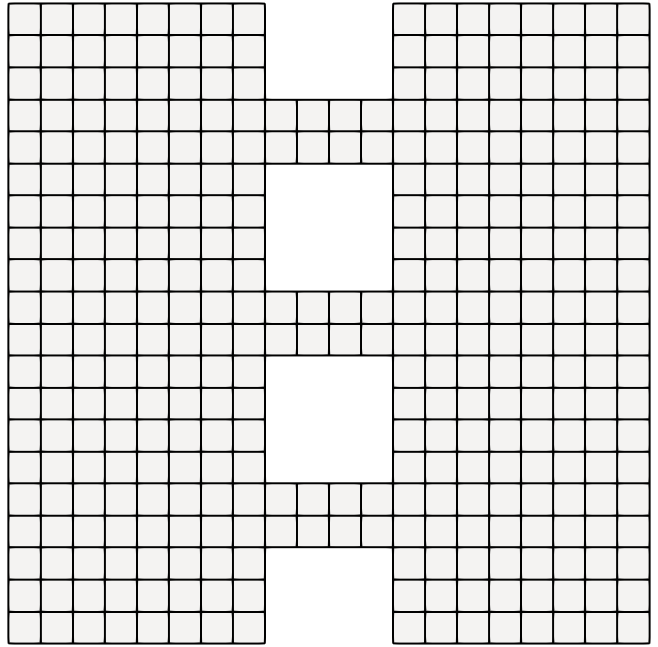
Figure 2: A uniform rectangular mesh with $\Delta t=0.1$ for the spatial domain $\Omega$.

We terminate the ALG2 algorithm when the error $err_{m}^{a}$ is less than $0.01$. The number of iterations needed for convergence for the 5 cases are recorded in Table 4, where we find Case 2 has the smallest number of iterations.

	Case 1	Case 2	Case 3	Case 4	Case 5
iterations	780	72	245	503	552

Table 4: Example 4.2. Number of ALG2 iterations for each case.

Snapshots of the density contour at different times are shown in Figure 3. The effects of different interaction cost functions on the density profile are clearly observed.

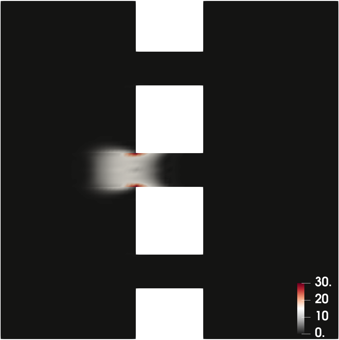
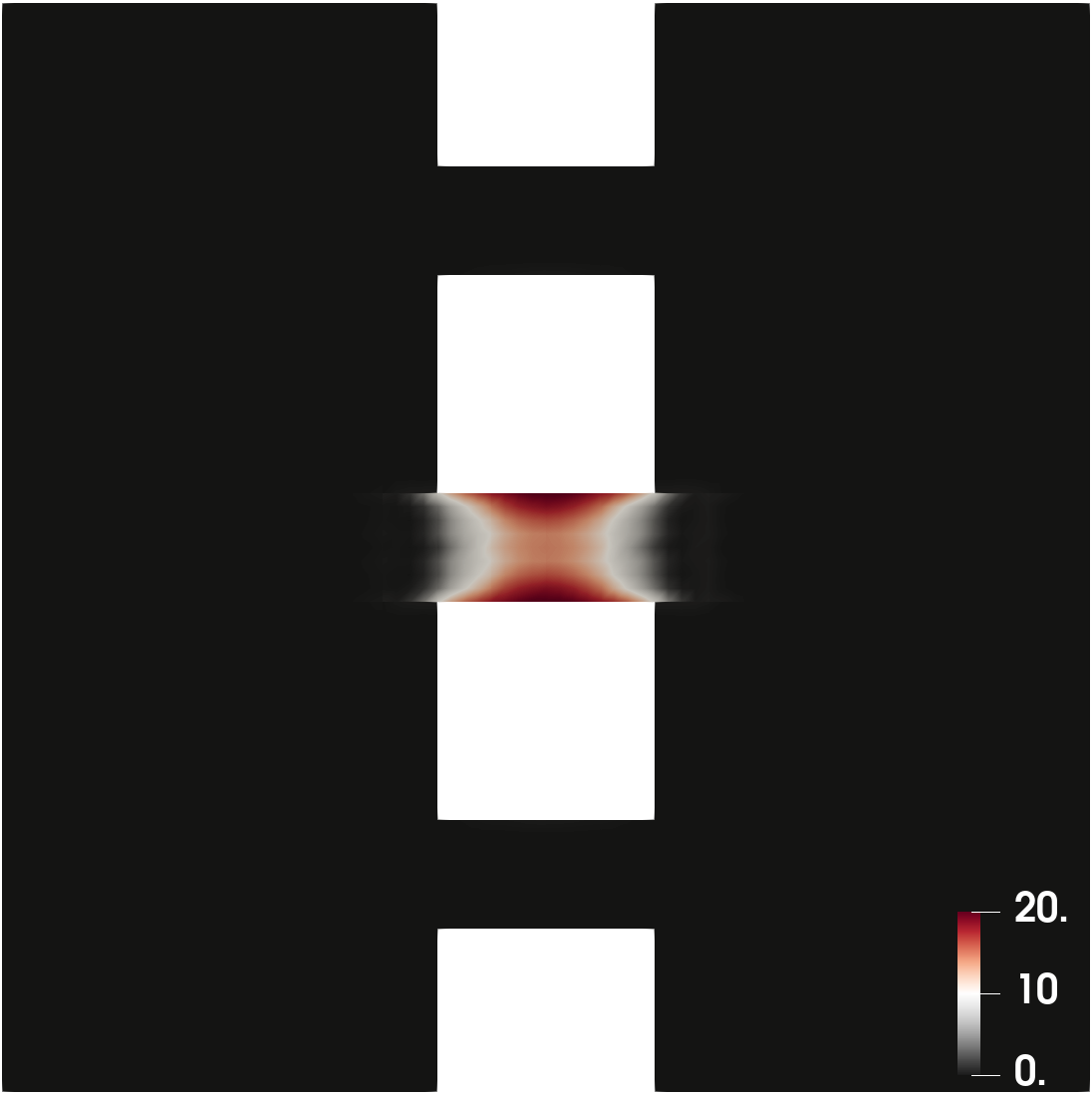
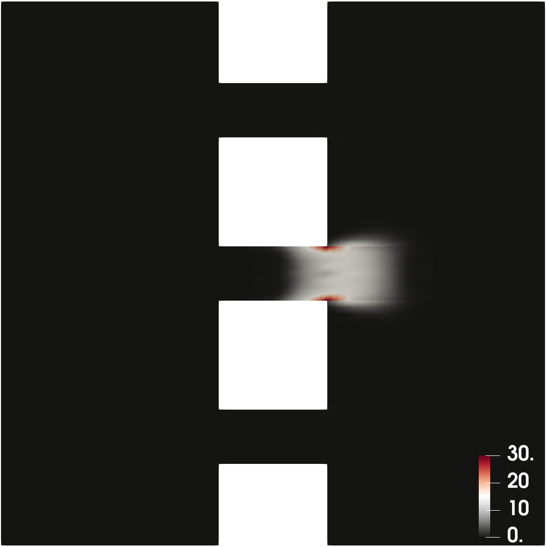
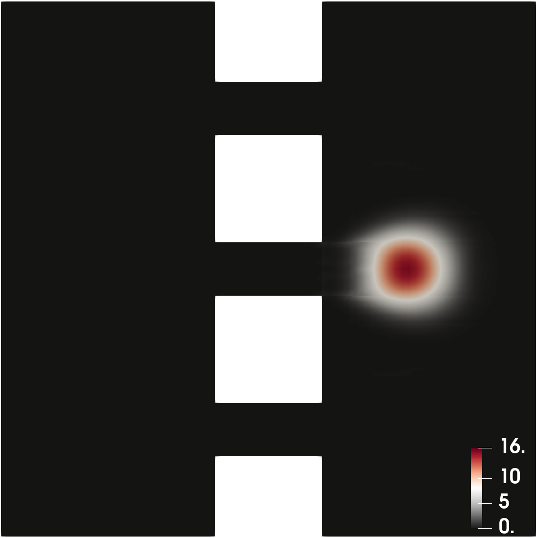
(a) Case 1

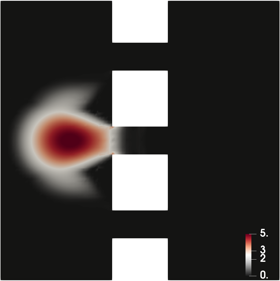
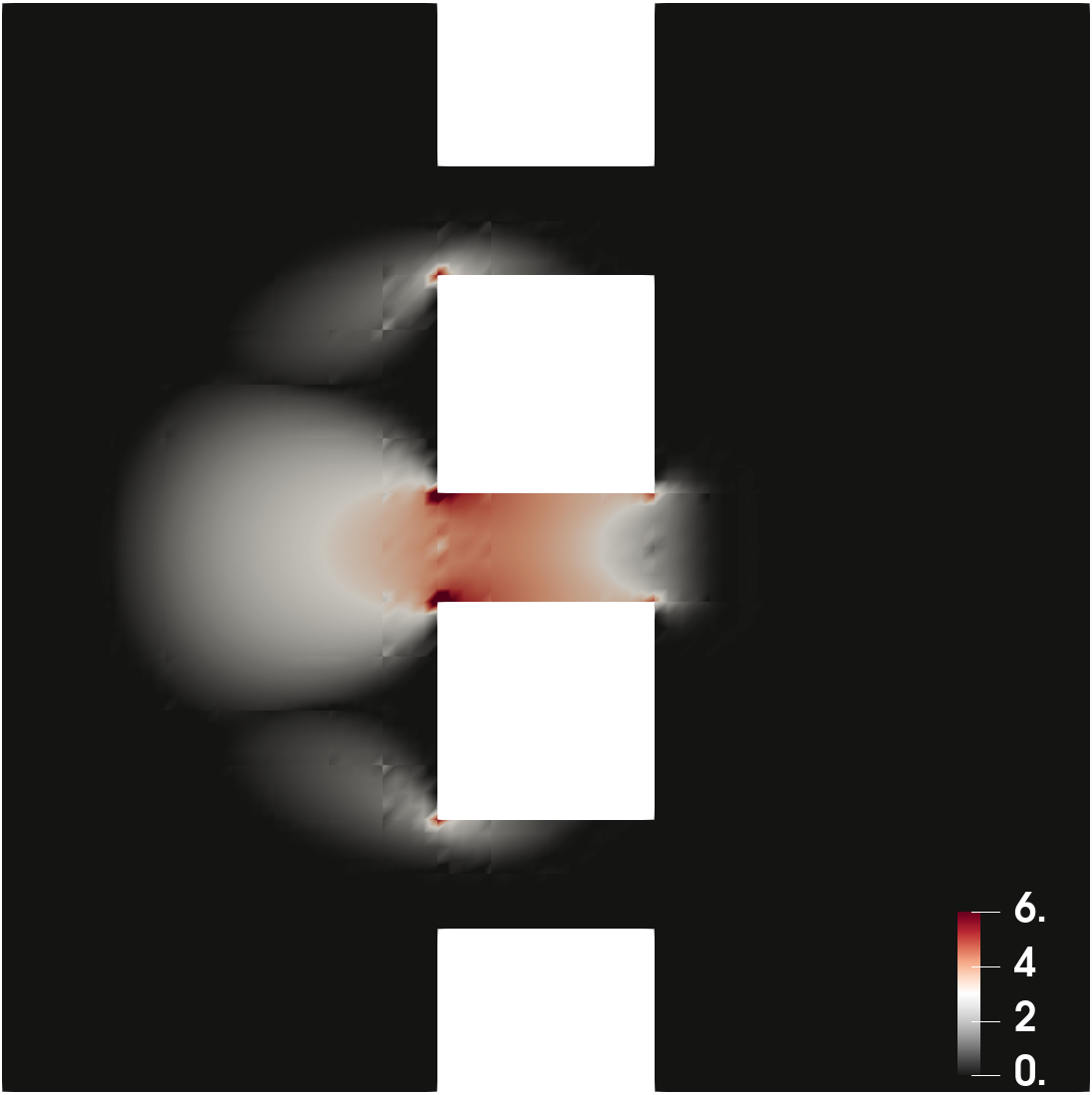
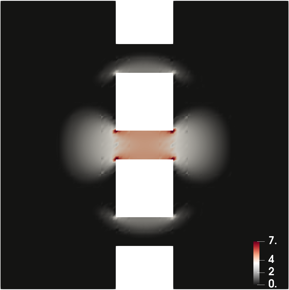
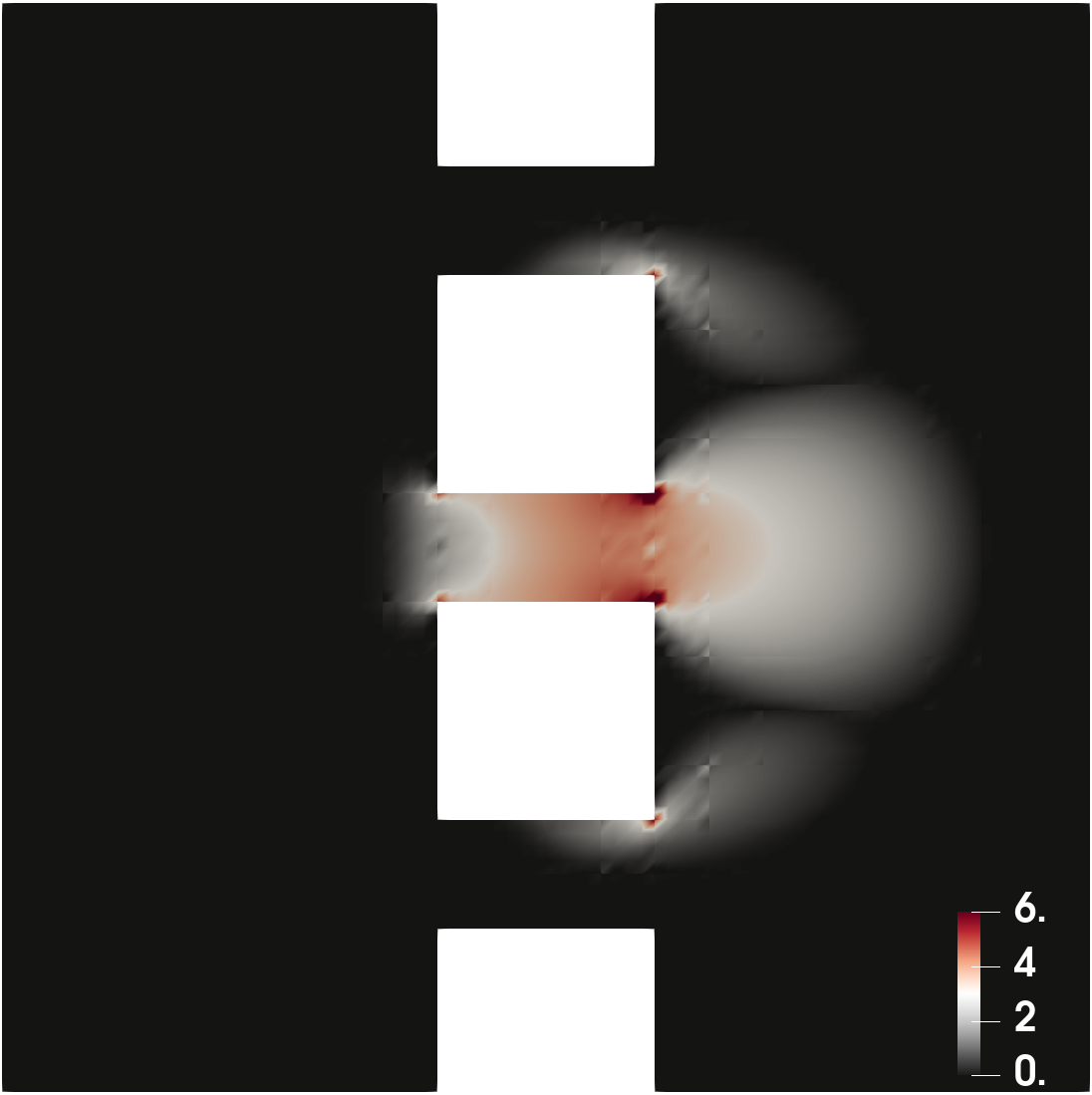
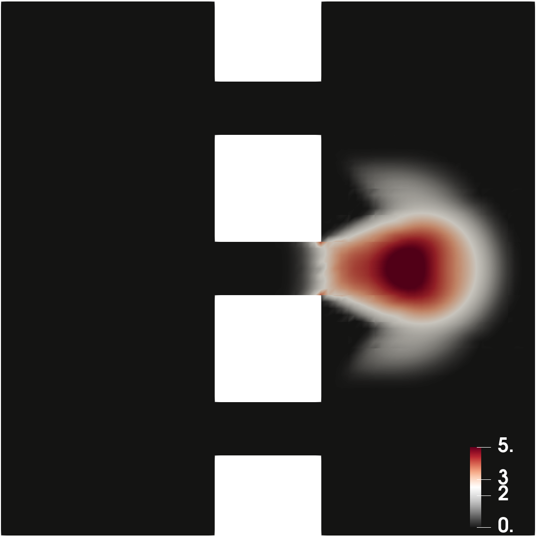
(b) Case 2

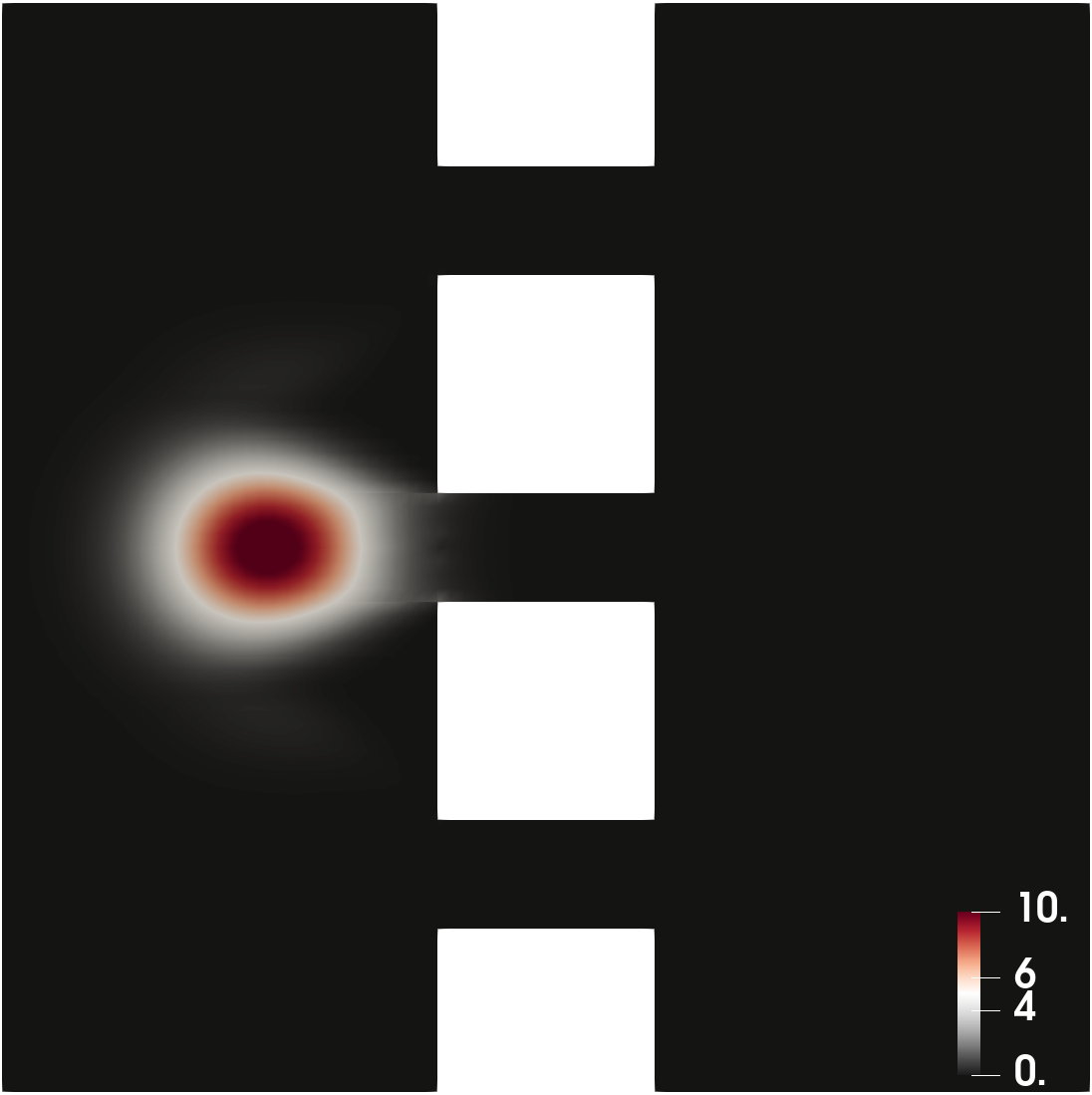
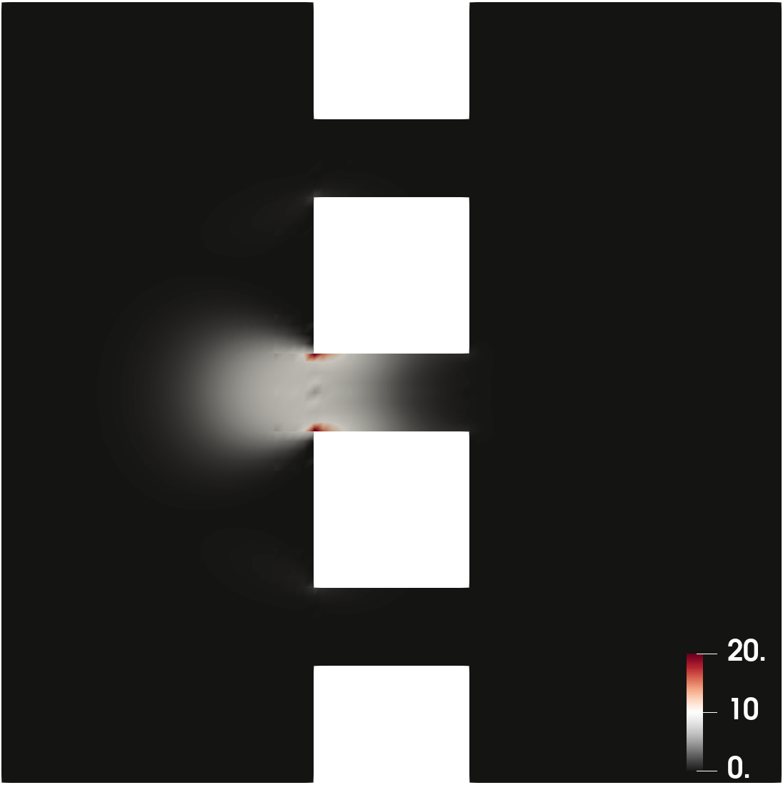
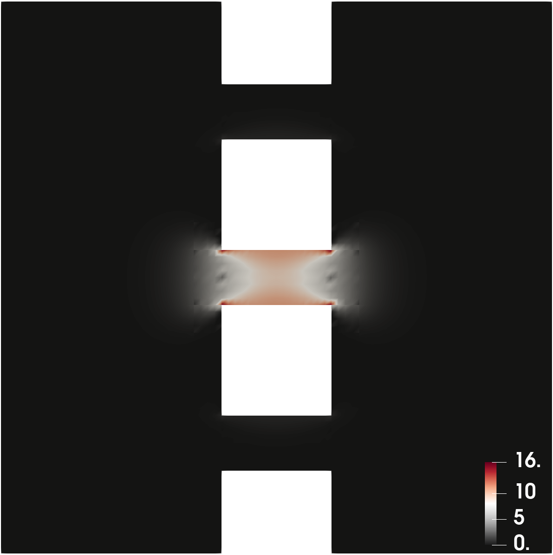
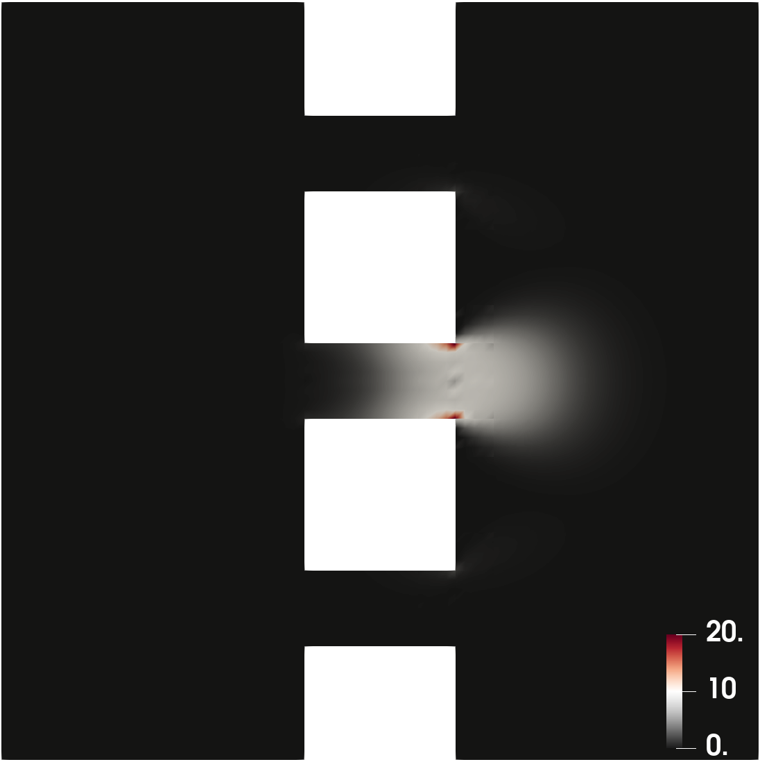
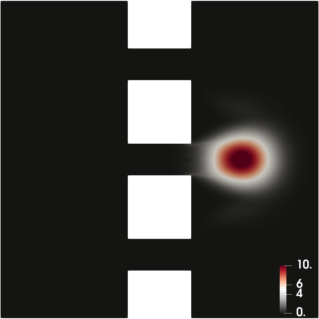
(c) Case 3

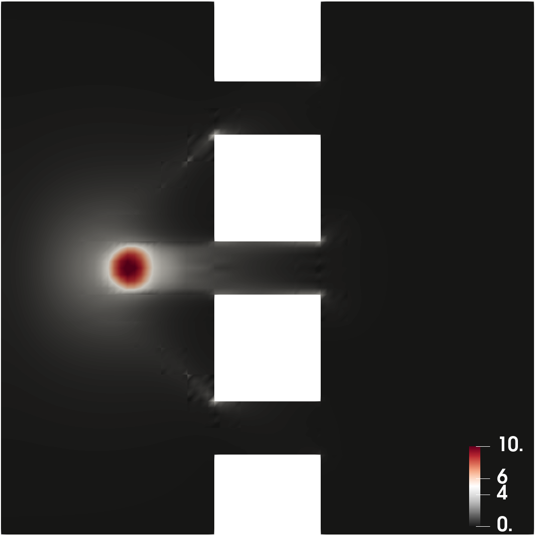
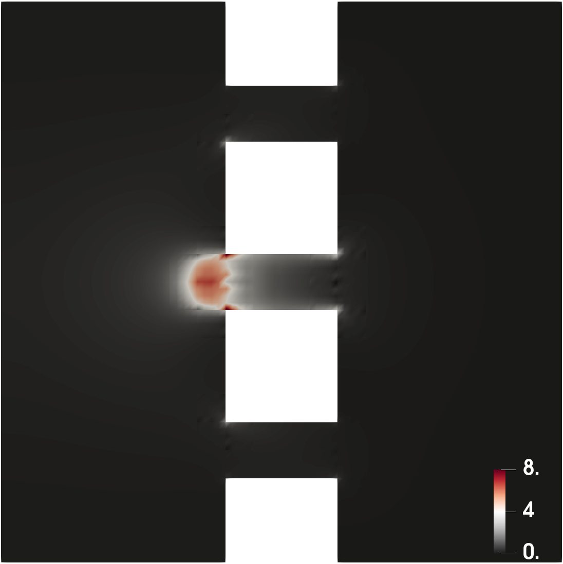
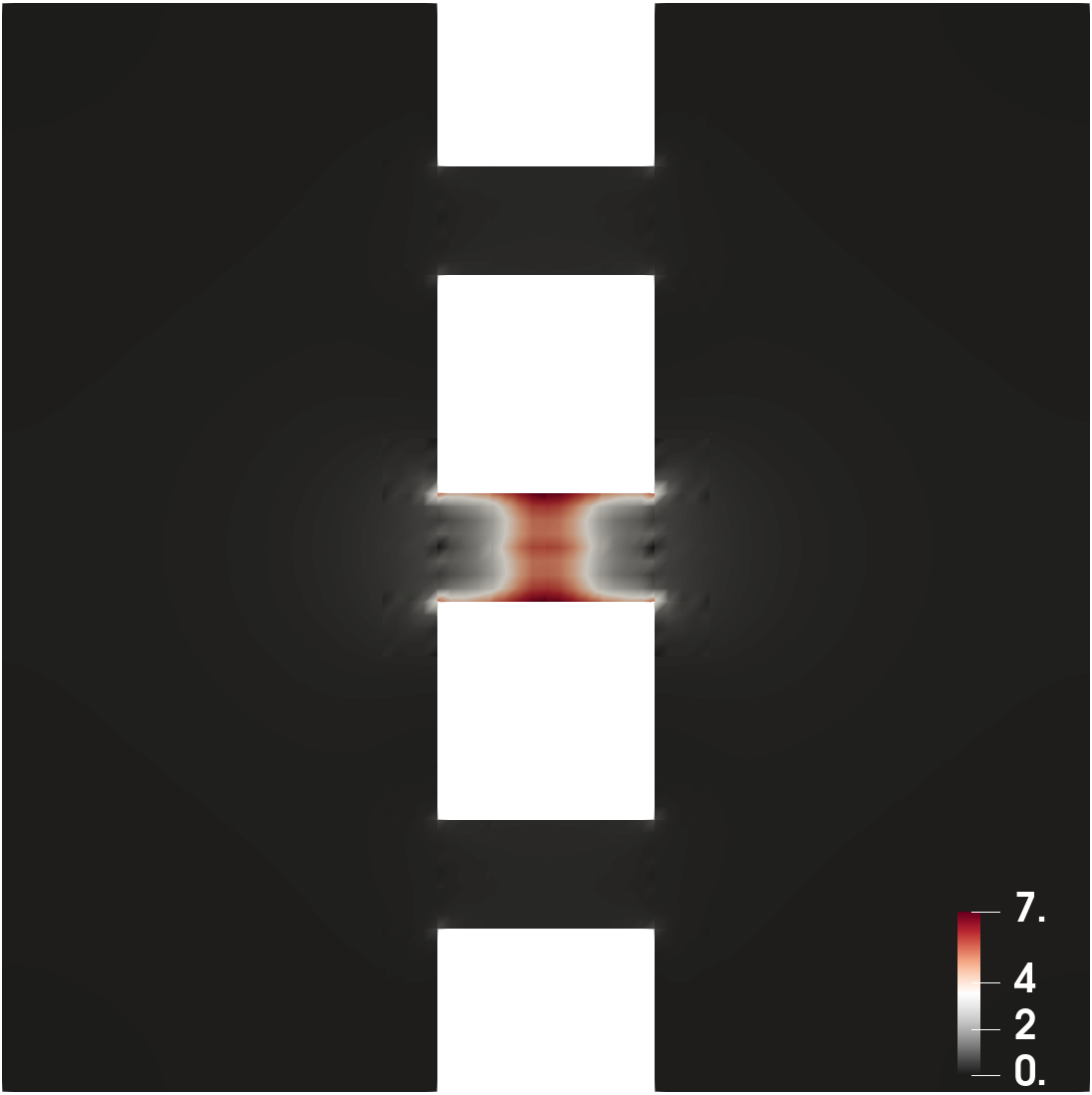
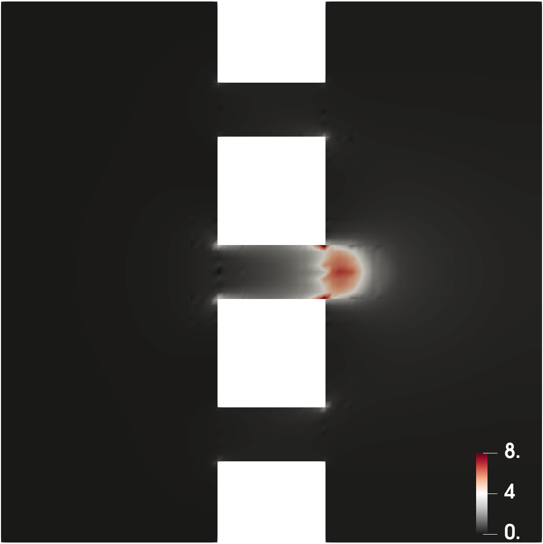
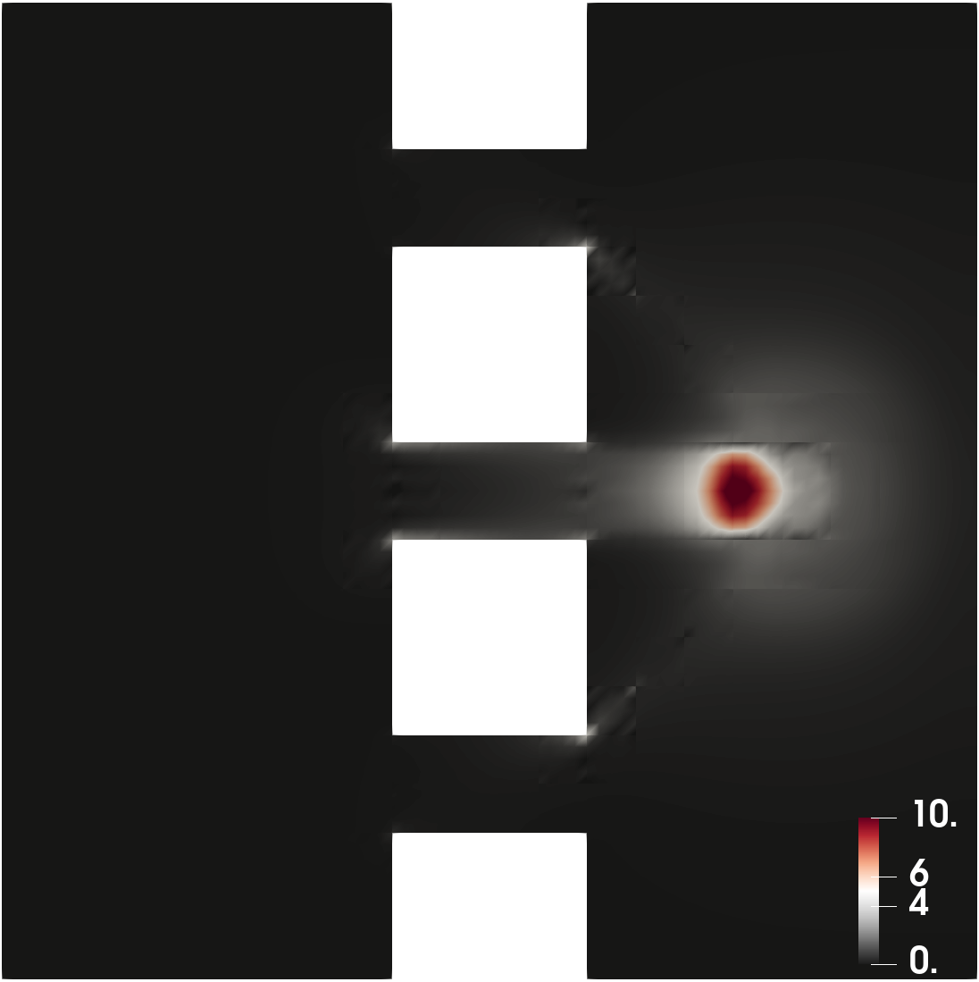
(d) Case 4

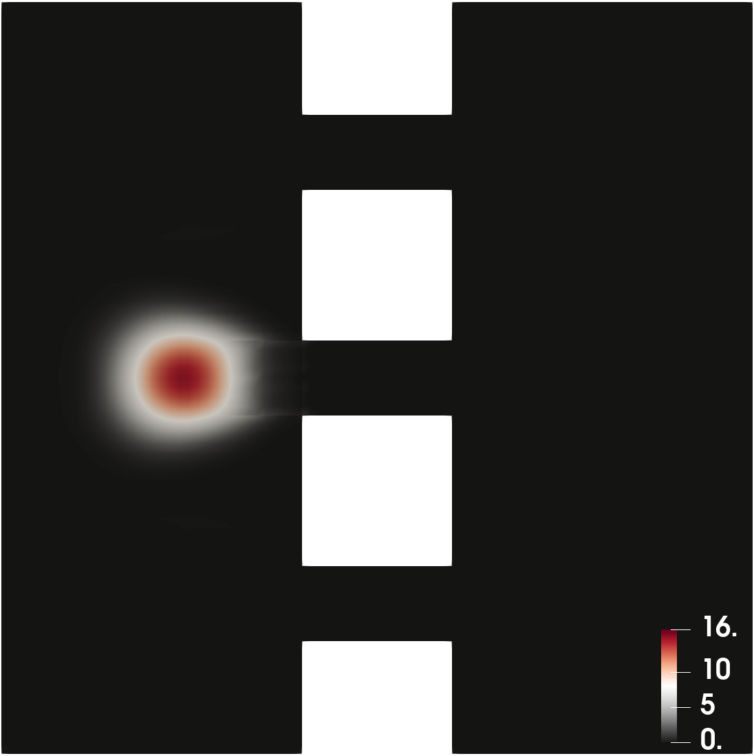
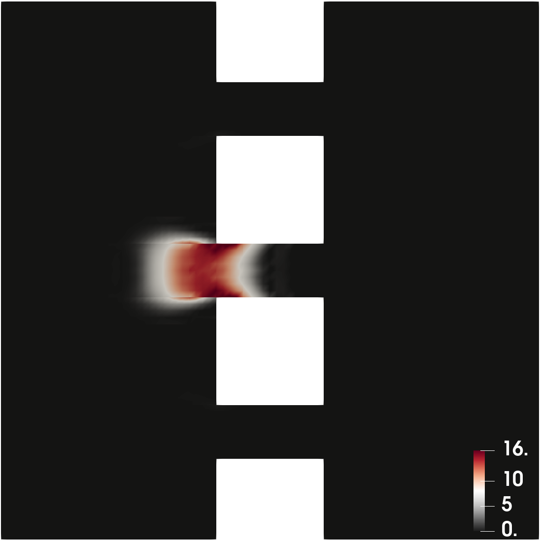
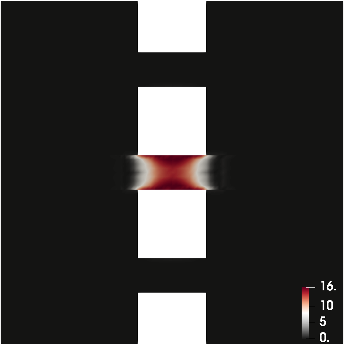
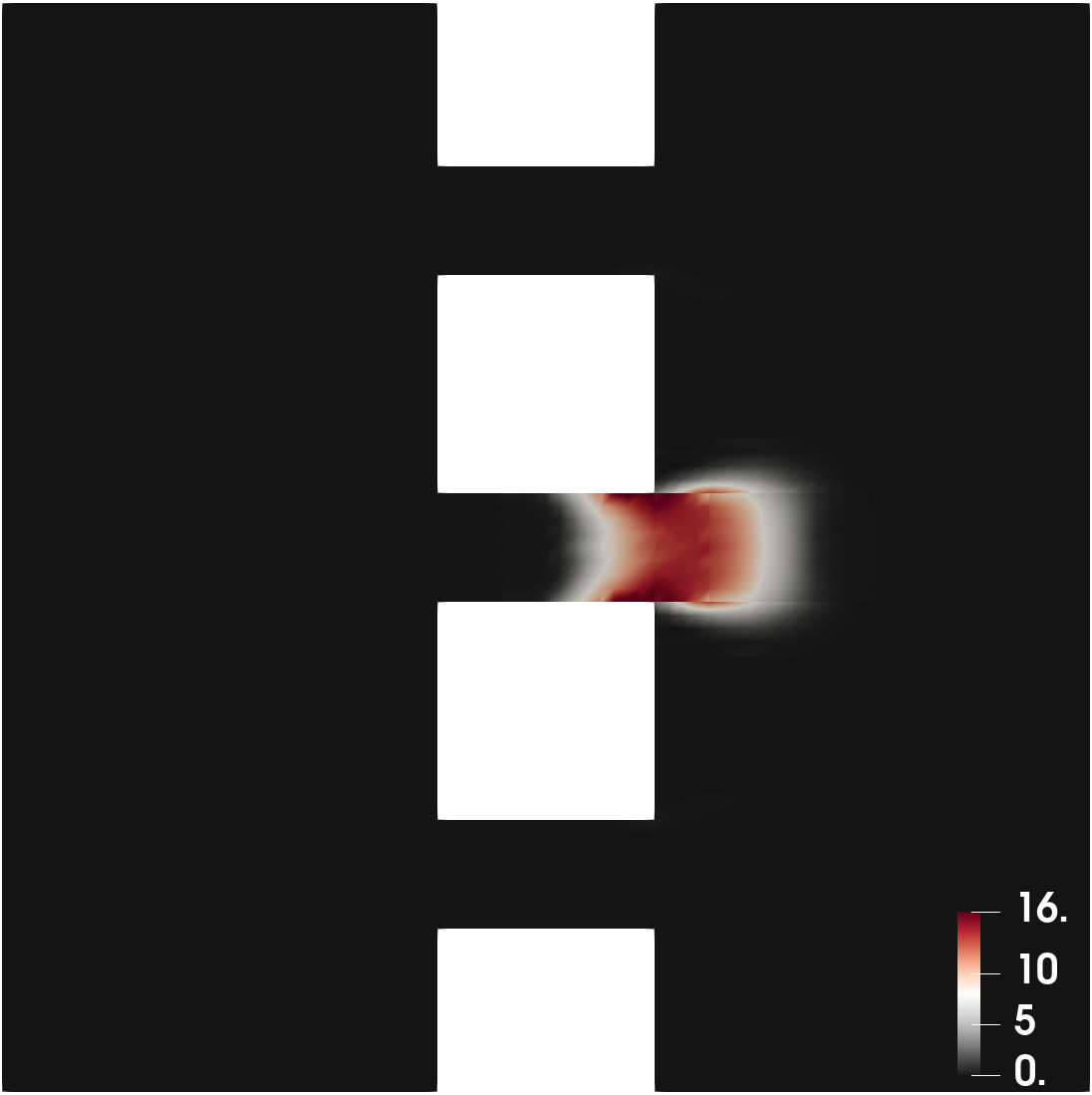
(e) Case 5

Figure 3: Example 4.2. Snapshots of $\rho$ at $t=0.1,0.3,0.5,0.7,0.9$ (left to right).

4.3 MFG with obstacles

We consider a similar setting as in Example 4.2, where we consider a MFG problem with terminal cost

$$\Gamma(\rho):=\begin{cases}\frac{1}{2}(\rho-\rho_{T})^{2}&\text{ if }\rho\geq 0,\\ +\infty&\text{ otherwise,}\end{cases}$$

where the target density

$$\rho_{T}:=\frac{1}{2\pi\sigma^{2}}\left(\exp(-\frac{1}{2\sigma^{2}}|\bm{x}-(0.65,0.3)|^{2})+\exp(-\frac{1}{2\sigma^{2}}|\bm{x}-(0.65,-0.3)|^{2})\right)$$

with $\sigma=0.1$. Note that we allow $\rho_{T}$ and $\rho_{0}$ to have different total masses here.

We apply the scheme (3.16) with polynomial degree $k=3$ on the same mesh as in Example 4.2, and use the same stopping criterion. The number of iterations needed for convergence for the 5 cases are recorded in Table 5, where again we find Case 2 has the smallest number of iterations.

	Case 1	Case 2	Case 3	Case 4	Case 5
iterations	3510	82	476	503	798

Table 5: Example 4.3. Number of ALG2 iterations for each case.

Snapshots of the density contour at different times are shown in Figure 4. The results are similar to those in Example 4.2, where different interaction cost function leads to different density evolution.

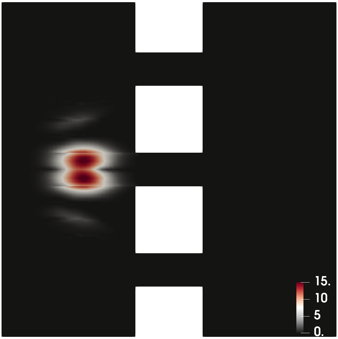
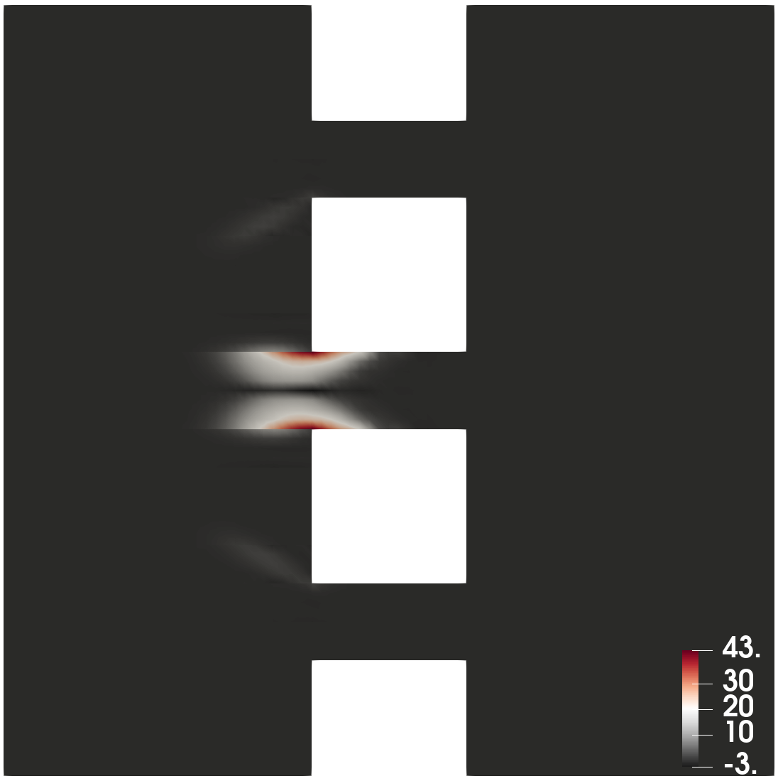
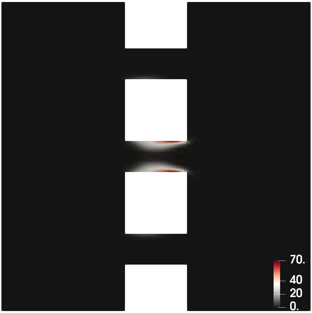
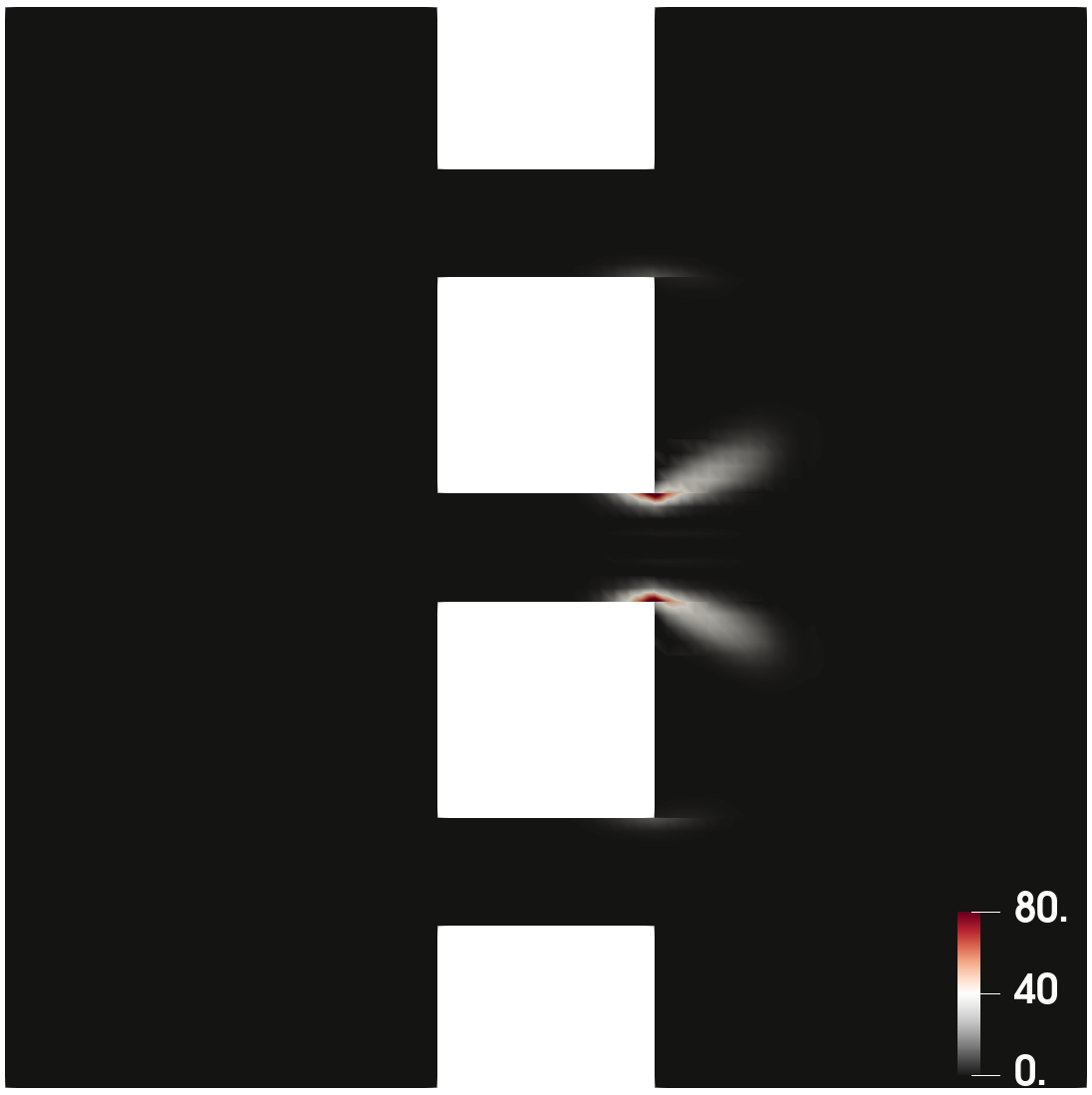
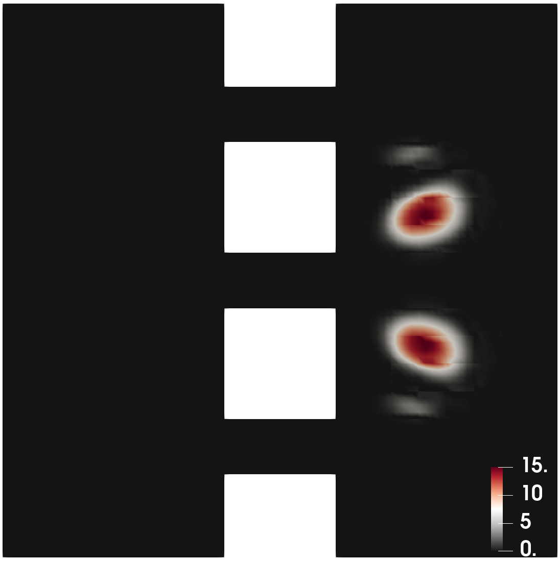
(a) Case 1

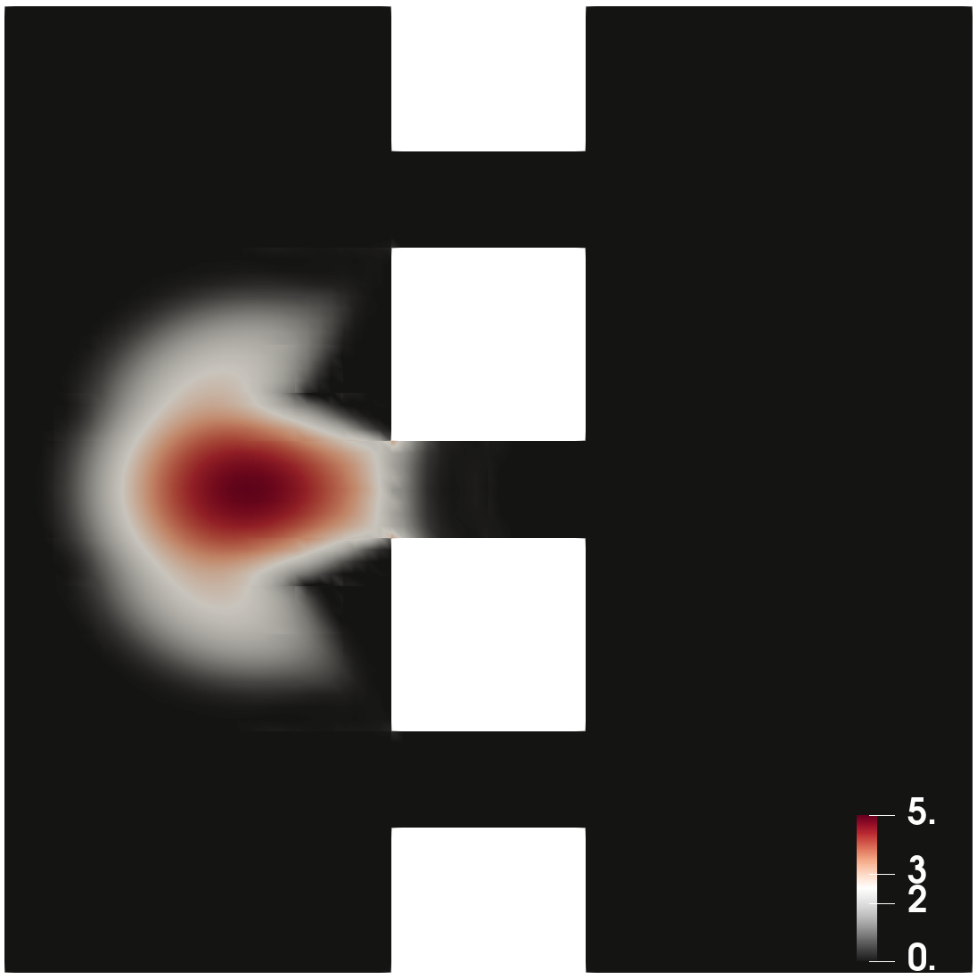
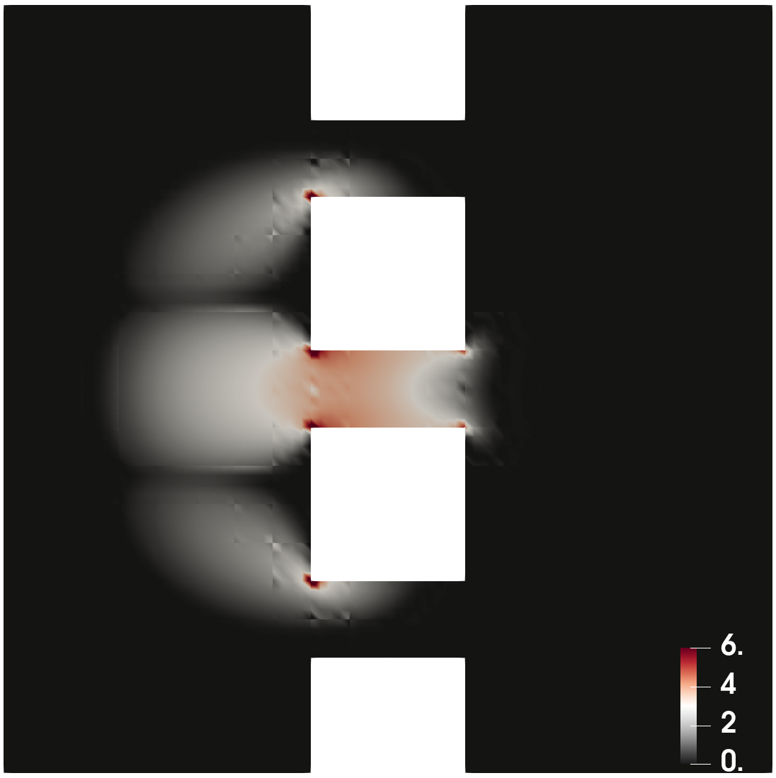
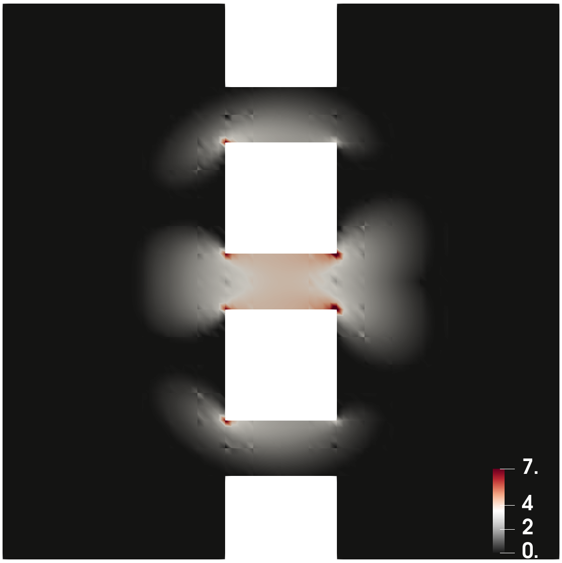
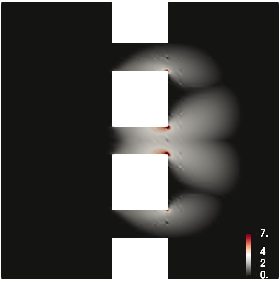
(b) Case 2

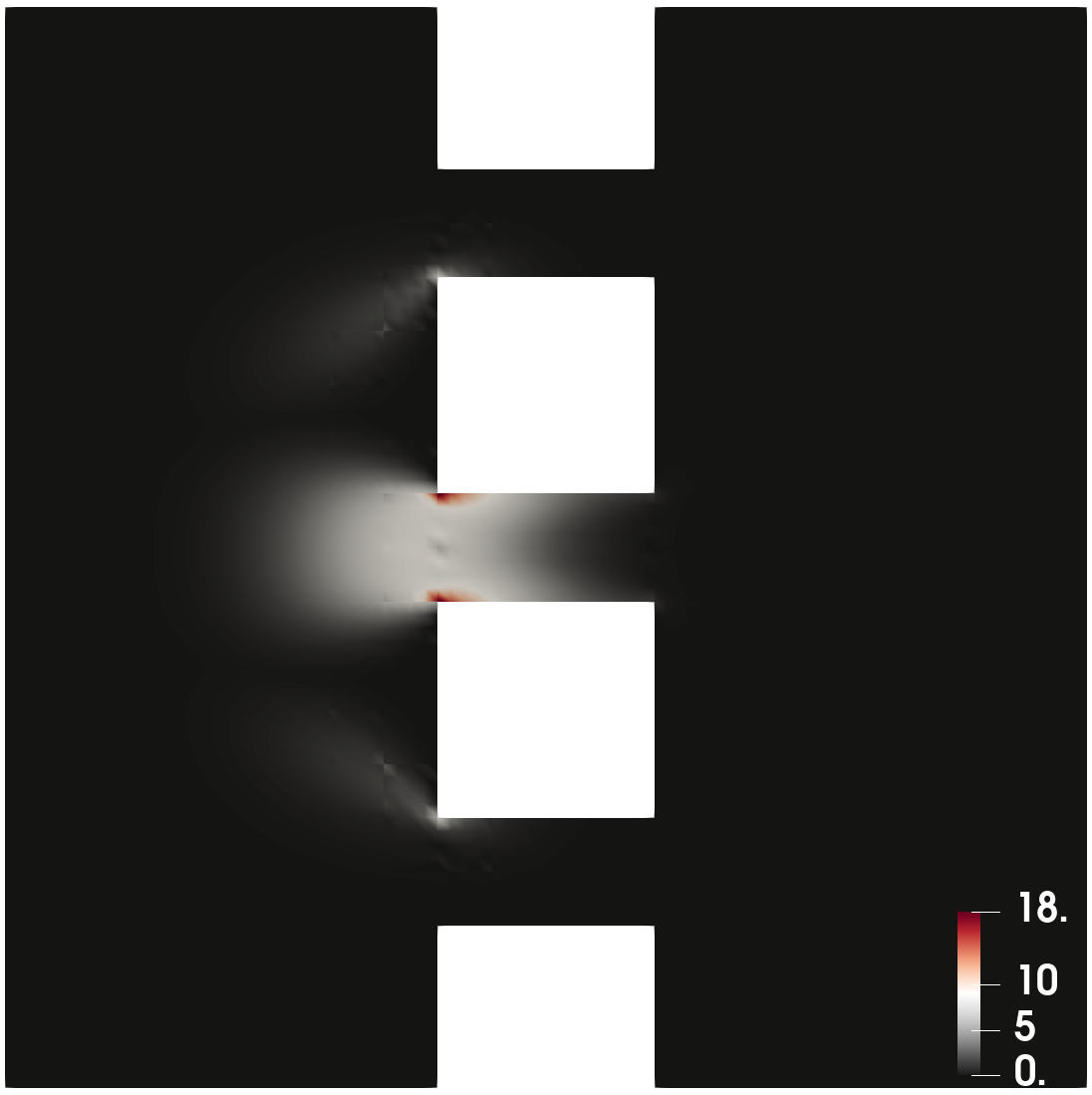
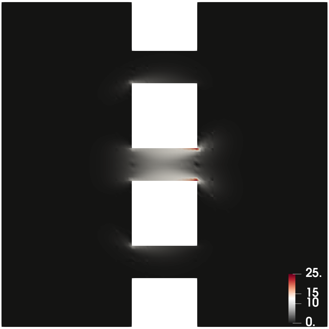
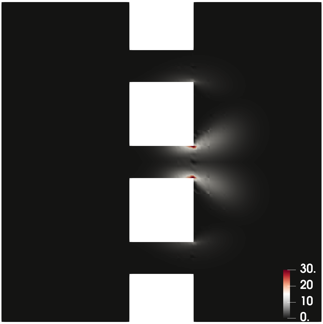
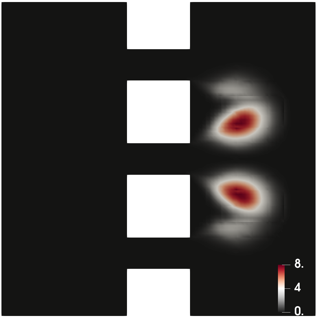
(c) Case 3

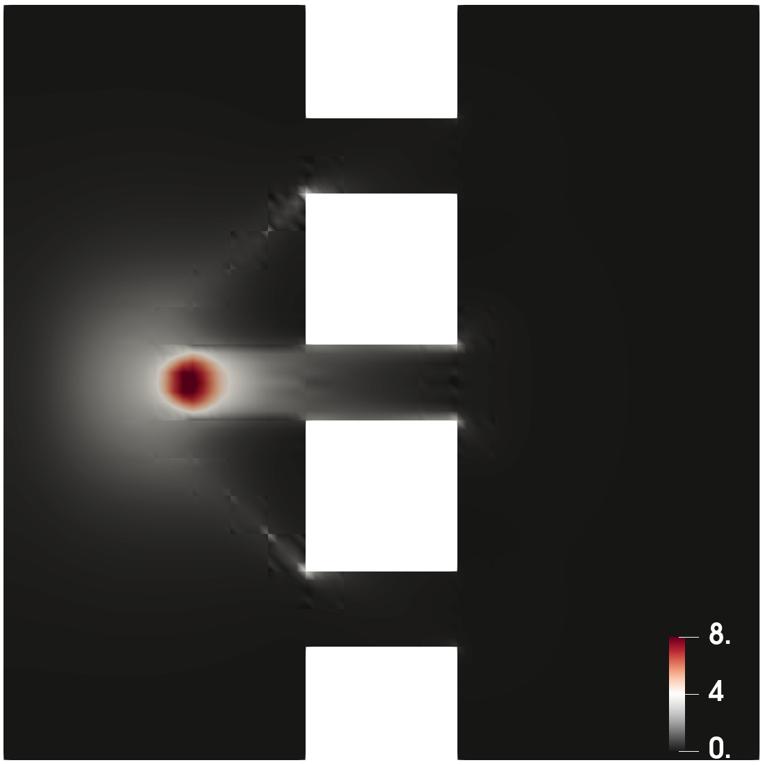
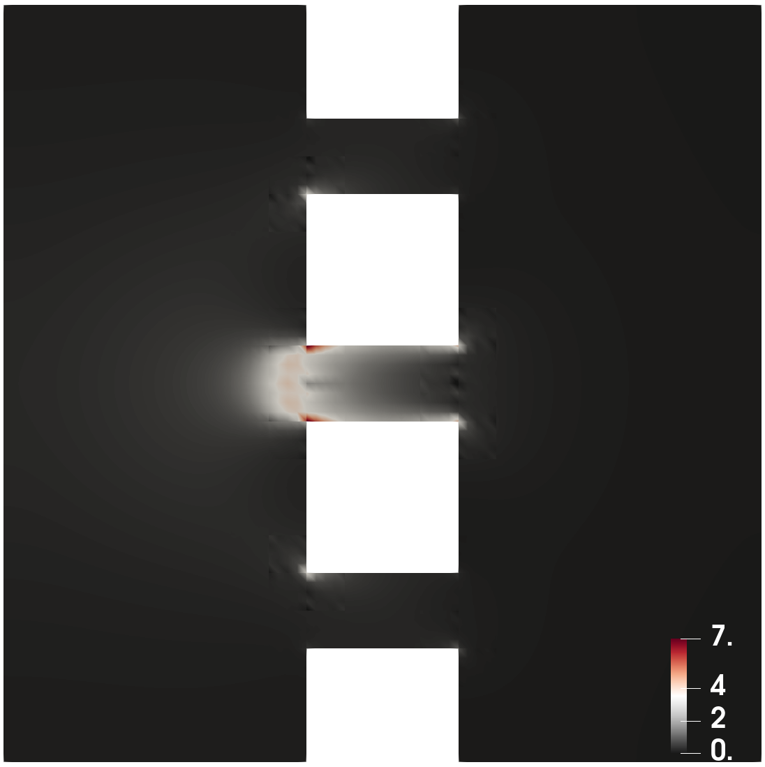
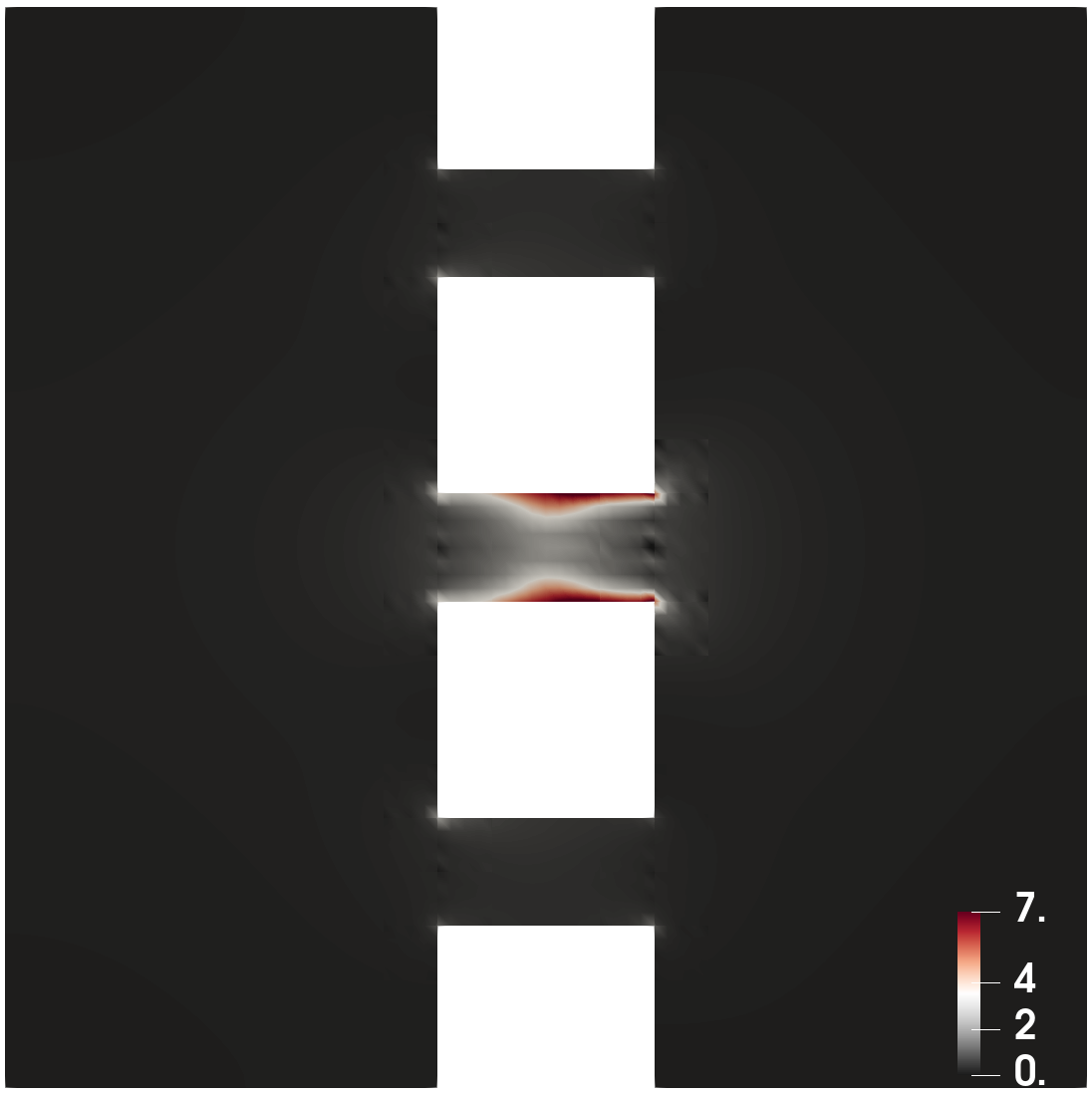
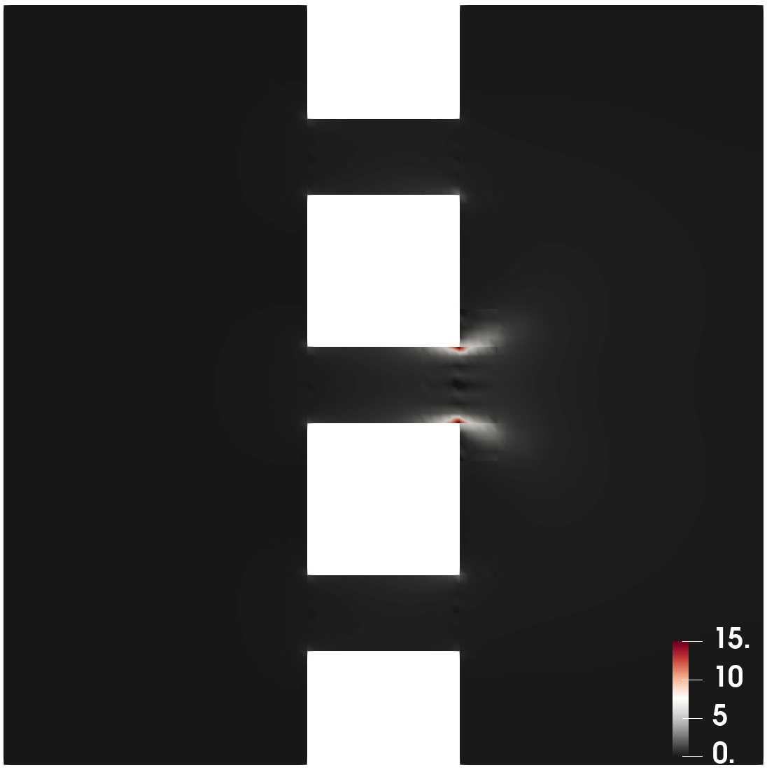
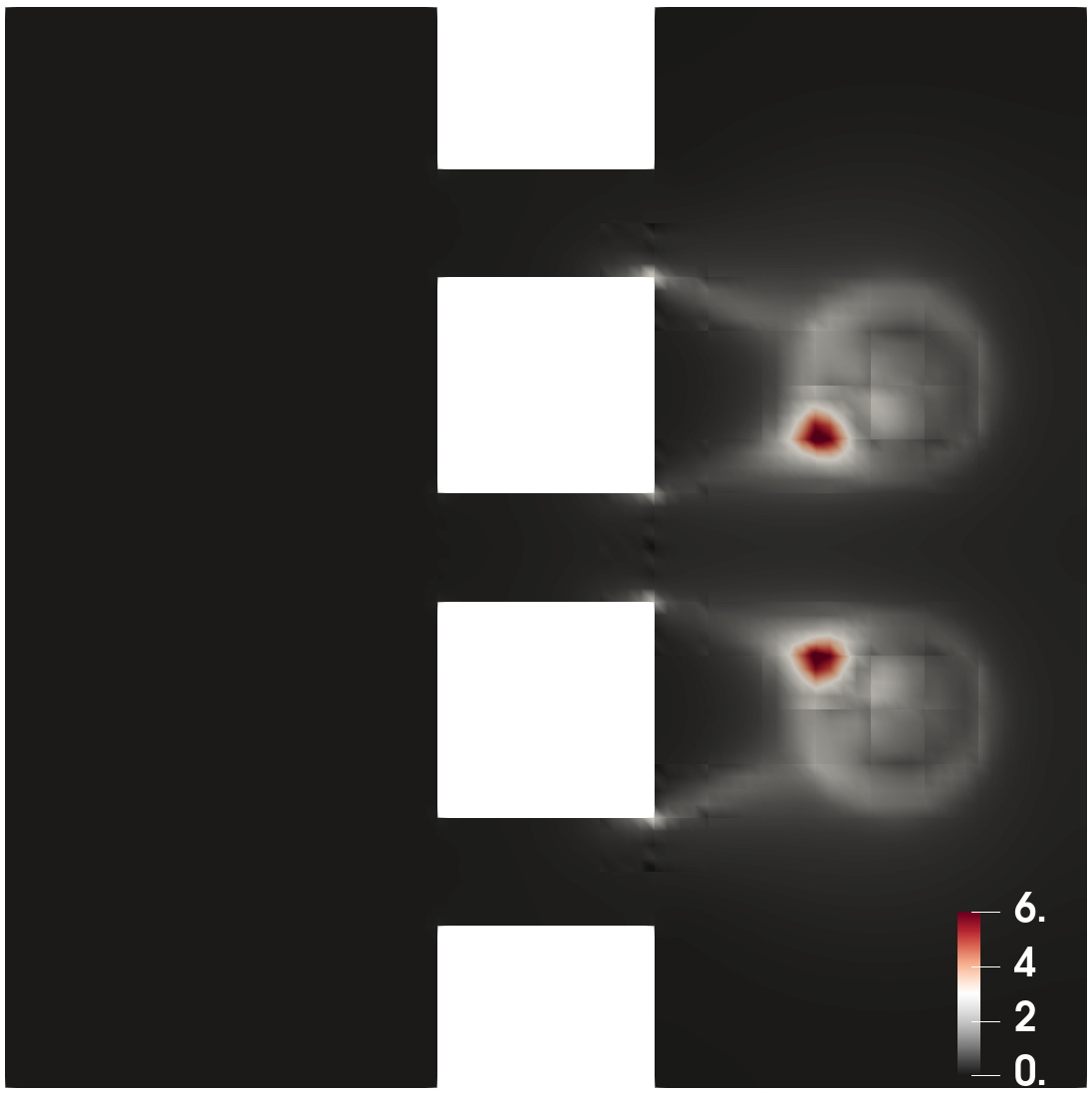
(d) Case 4

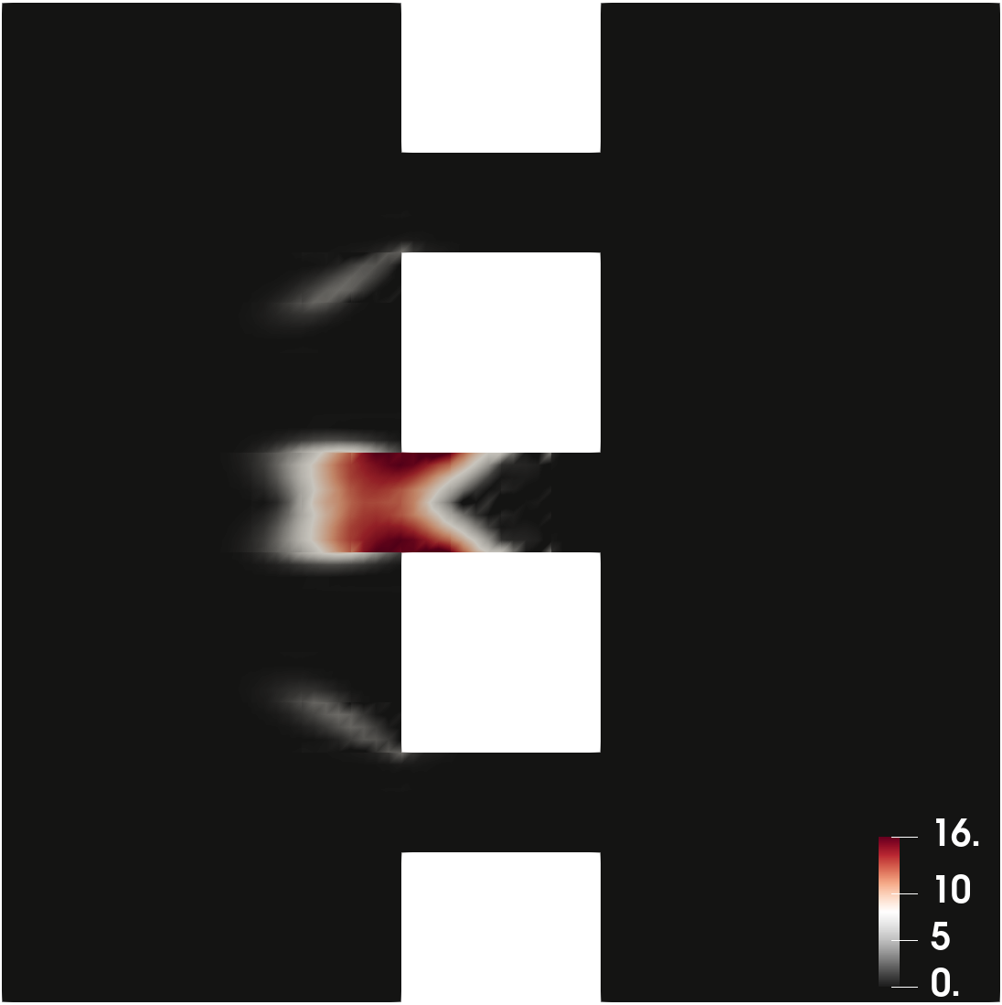
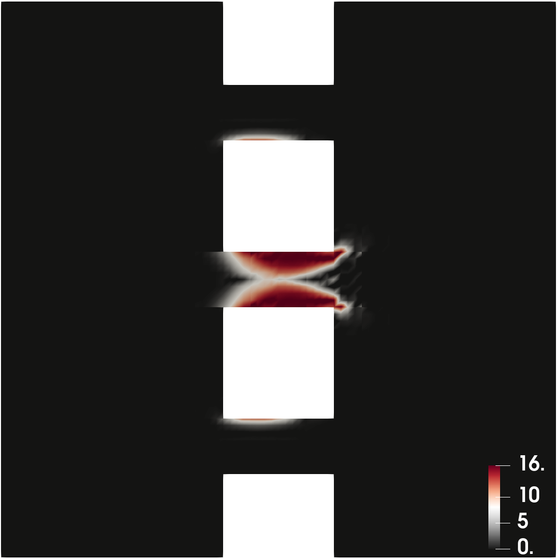
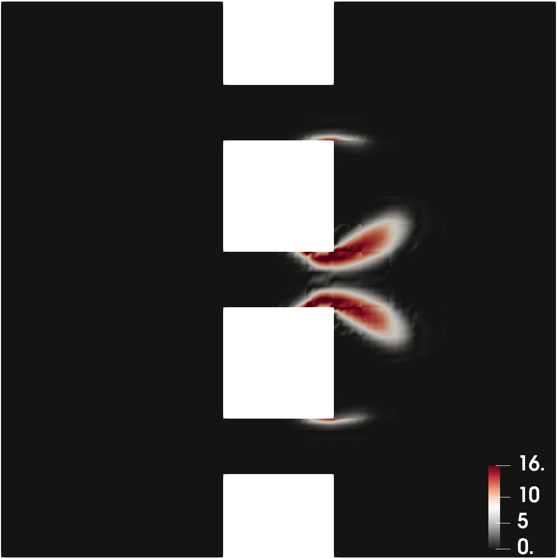
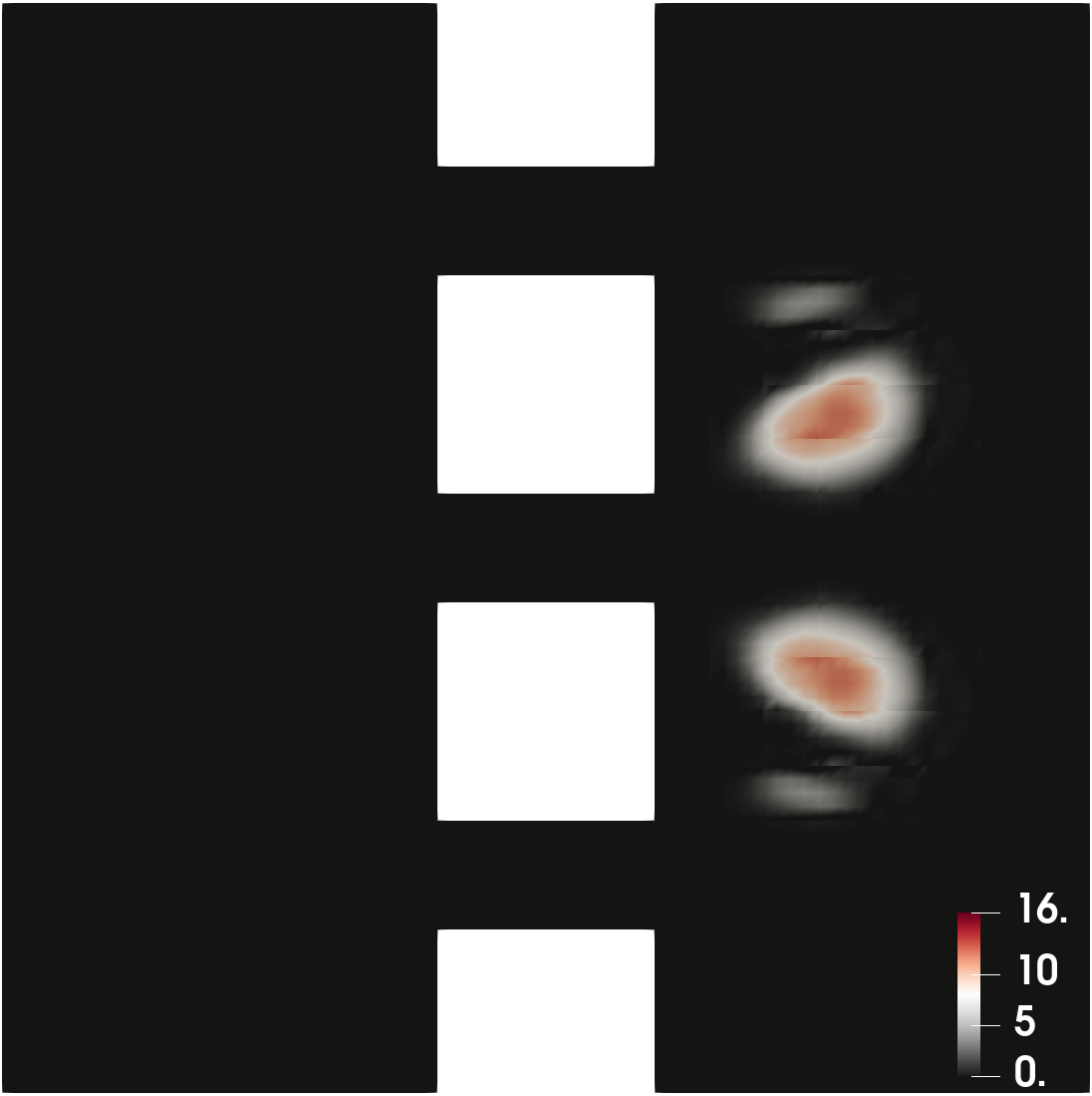
(e) Case 5

Figure 4: Example 4.3. Snapshots of $\rho$ at $t=0.1,0.3,0.5,0.7,0.9$ (left to right).

4.4 MFP between mascot images

Our last example concerns with OT and MFP (2.3) between images. The initial or terminal densities are normalized images of athletics mascots from University of Notre Dame (Leprechaun), UCLA (Brunins), and University of South Carilina (Gamecocks); see Figure 5. The spatial domain is a unit square $\Omega=[0,1]\times[0,1]$, and the initial/terminal densities are normalized to have unit mass.

We apply the scheme (3.12) with polynomial degree $k=3$ on a structured hexahedral mesh of size $64\times 64\times 16$, where the time step size is $\Delta t=1/16$. Three set of initial/terminal density pairs are considered: (i) ND$\rightarrow$ UCLA where initial density is the ND image and terminal density is the UCLA image, (ii) UCLA$\rightarrow$ USC where initial density is the UCLA image and terminal density is the USC image, and (iii) USC$\rightarrow$ ND where initial density is the USC image and terminal density is the ND image. For each pair of data, we consider three choices of interaction cost, namely, Case 1: $A(\rho)=0$ (OT), Case 2: $A(\rho)=0.01\rho\log(\rho)$, and Case 3: $A(\rho)=0.01/\rho$. The ALG2 algorithm is terminated when $err_{m}^{a}$ is less than 0.001. The number of iterations needed for convergence are recorded in Table 6.

	Case 1	Case 2	Case 3
ND$\rightarrow$UCLA	2440	471	892
UCLA$\rightarrow$USC	1511	211	244
USC$\rightarrow$ND	3577	496	907

Table 6: Example 4.4. Number of ALG2 iterations for each case.

Snapshots of the density contour at different times are shown in Figure 6 for (i) ND$\rightarrow$ UCLA, in Figure 7 for (ii) UCLA$\rightarrow$ USC, and in Figure 8 for (iii) USC$\rightarrow$ ND. We observe in these figures that Case 1 (OT) produce the most sharp results for the density evolution, and that both interaction costs in Case 2/3 have a strong smoothing effect which blur the density profile, where Case 3 with $A(\rho)=0.01/\rho$ also leads to an everywhere positive density.

(a) ND (Leprechaun)

(b) UCLA (Bruins)

(c) USC (Gamecocks)

Figure 5: Example 4.4. Initial/final densities.

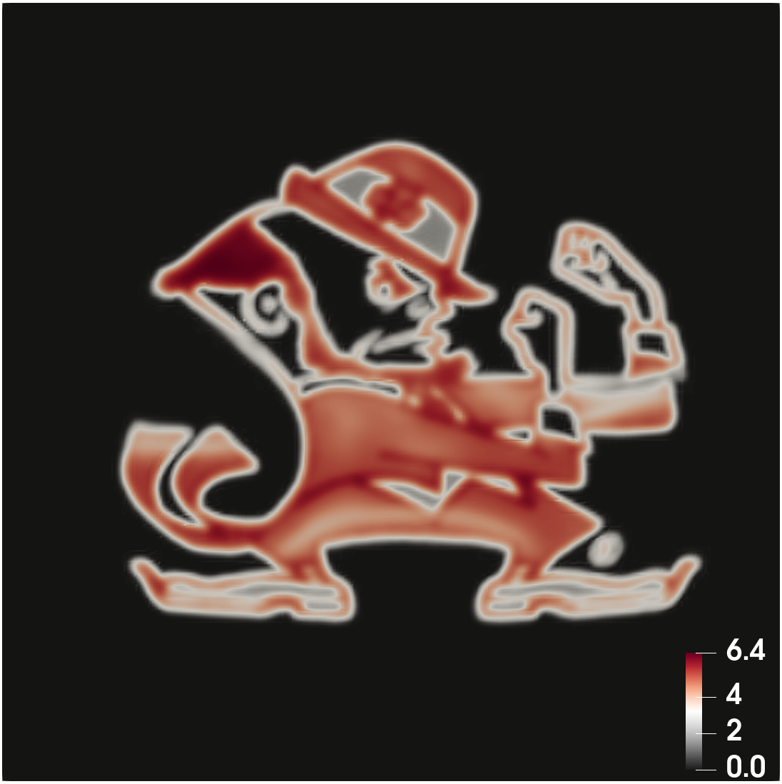
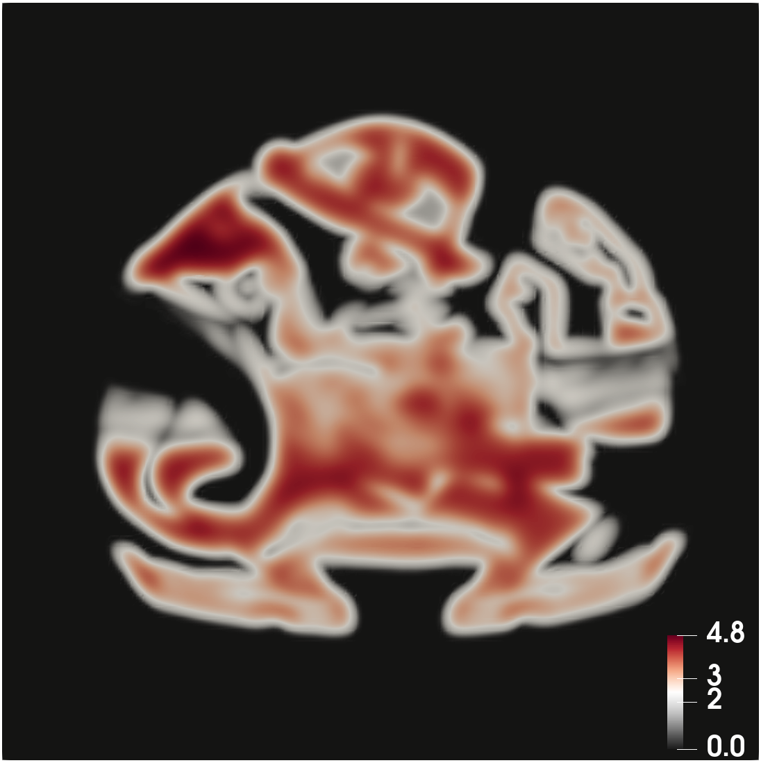
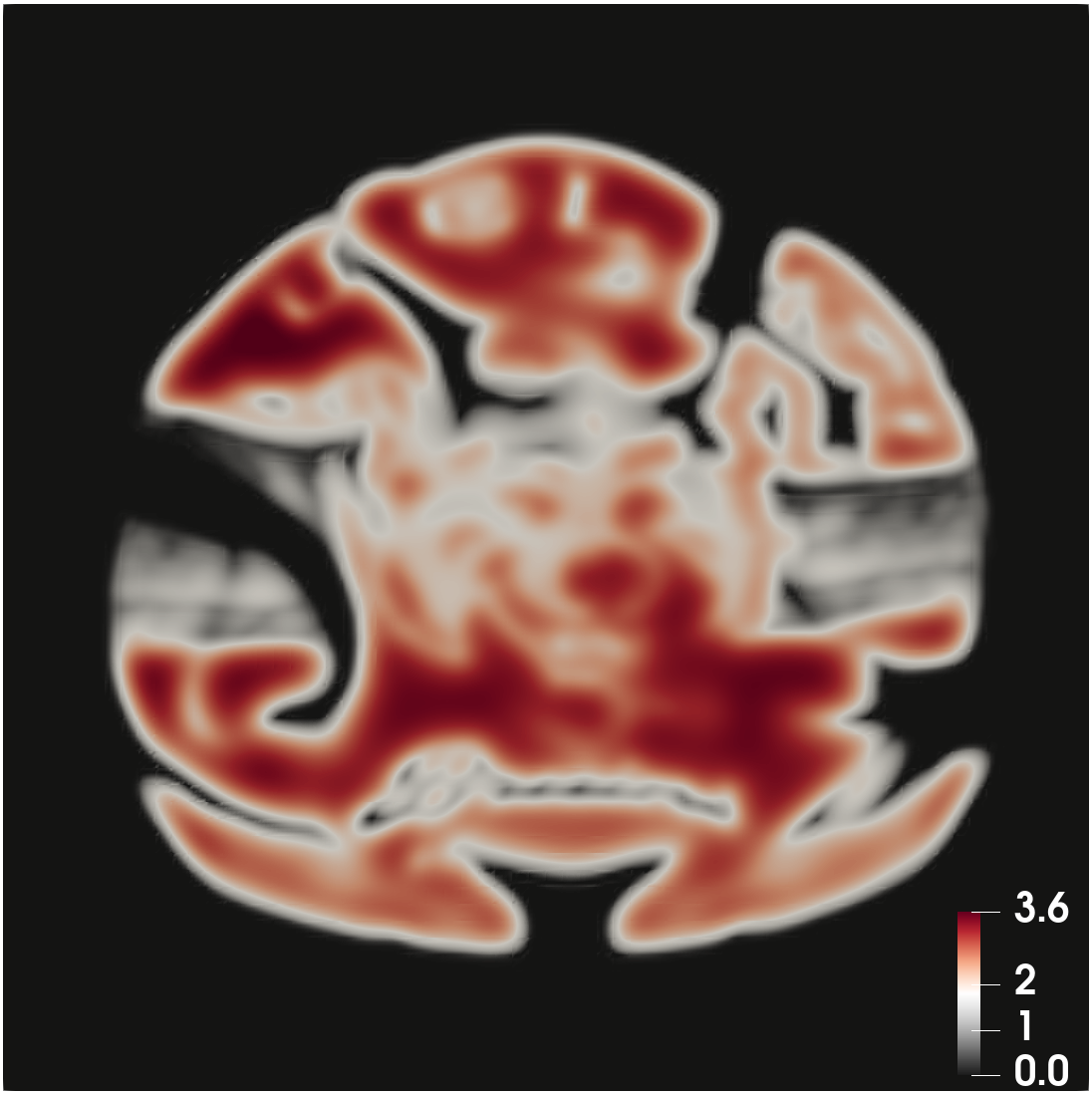
(a) Case 1: $A(\rho)=0$. ND $\rightarrow$ UCLA

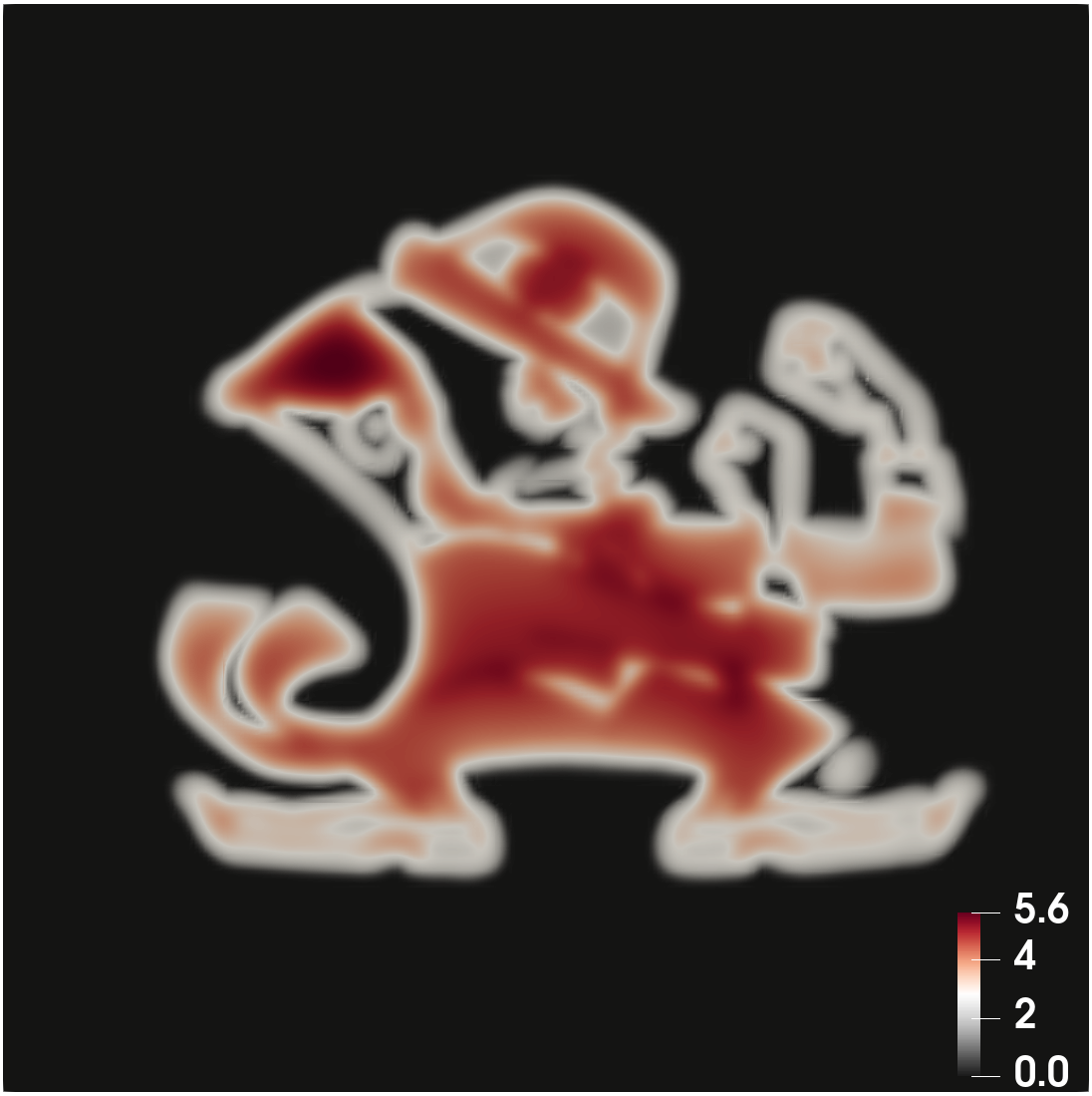
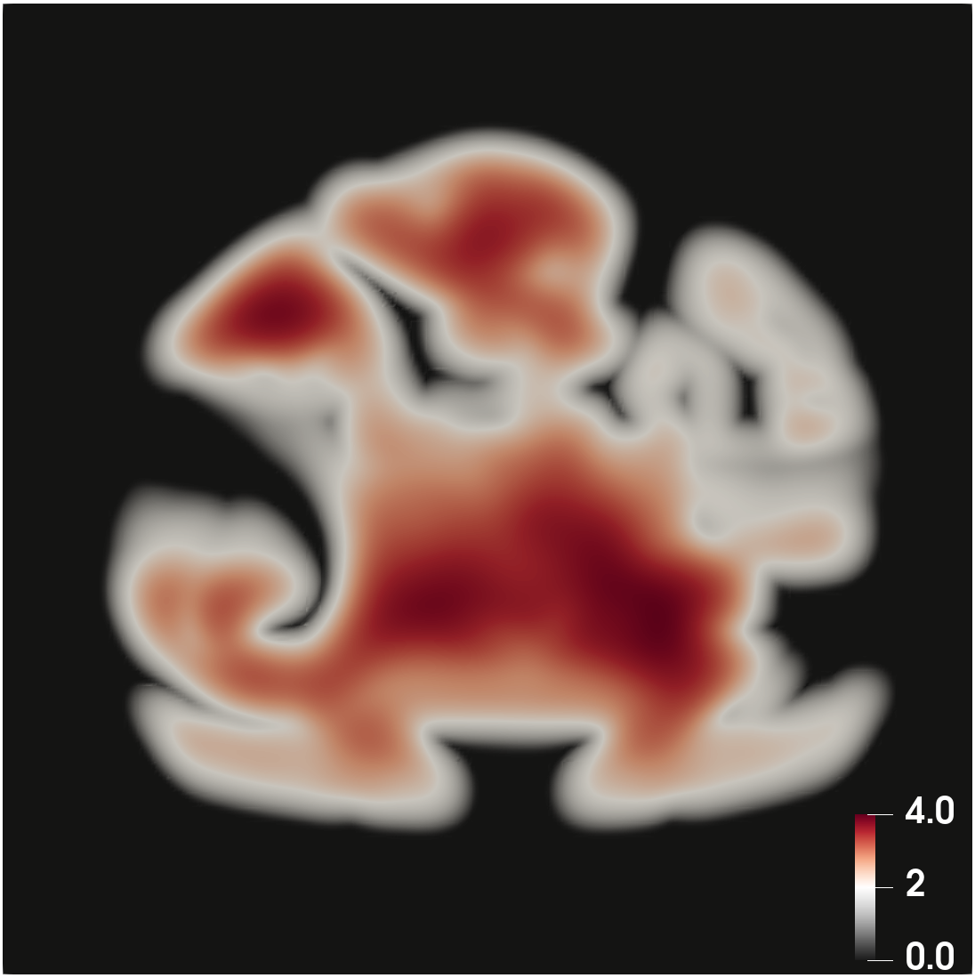
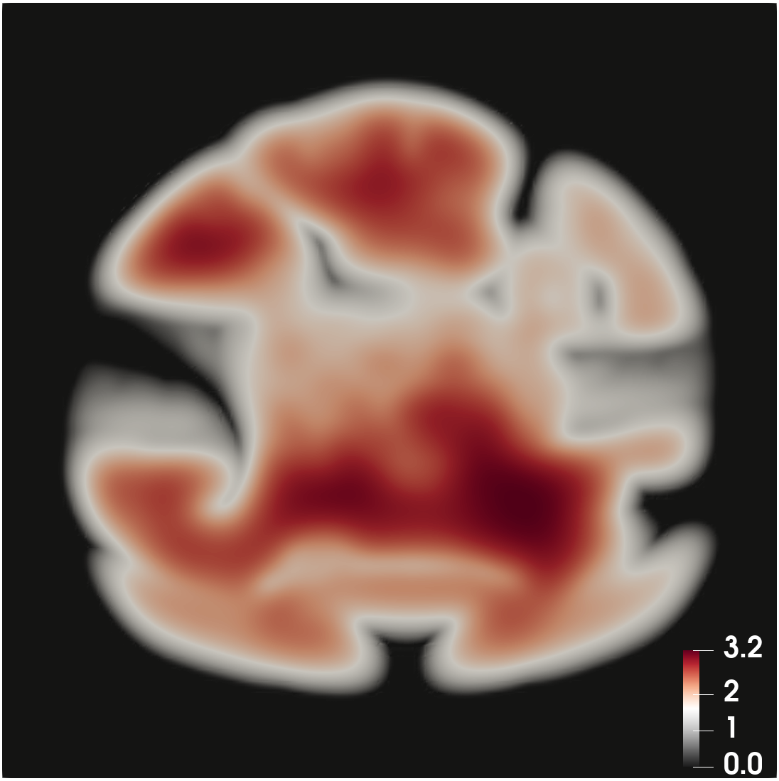
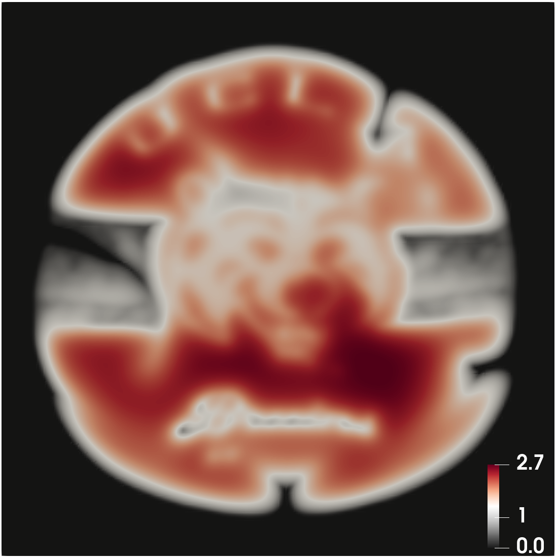
(b) Case 2: $A(\rho)=0.01\rho\log(\rho)$. ND $\rightarrow$ UCLA

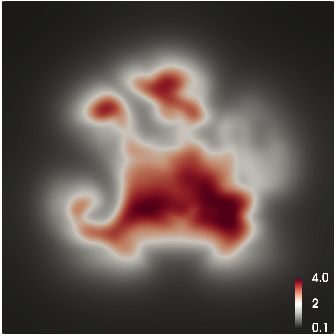
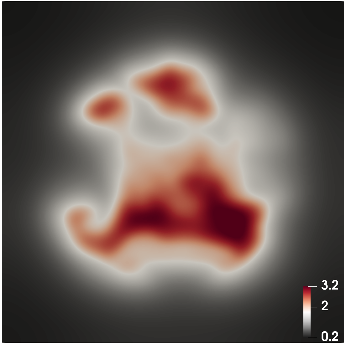
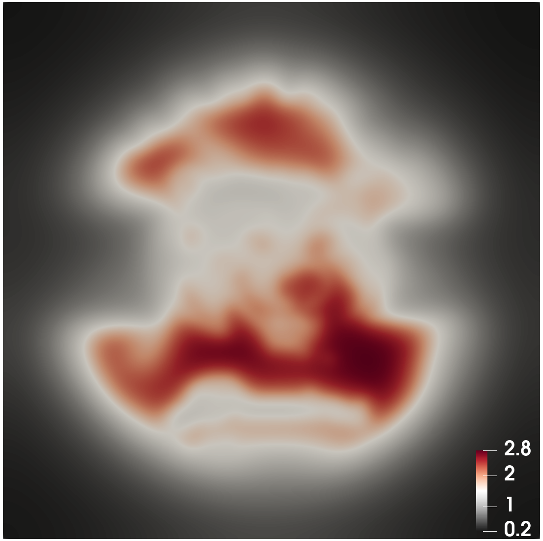
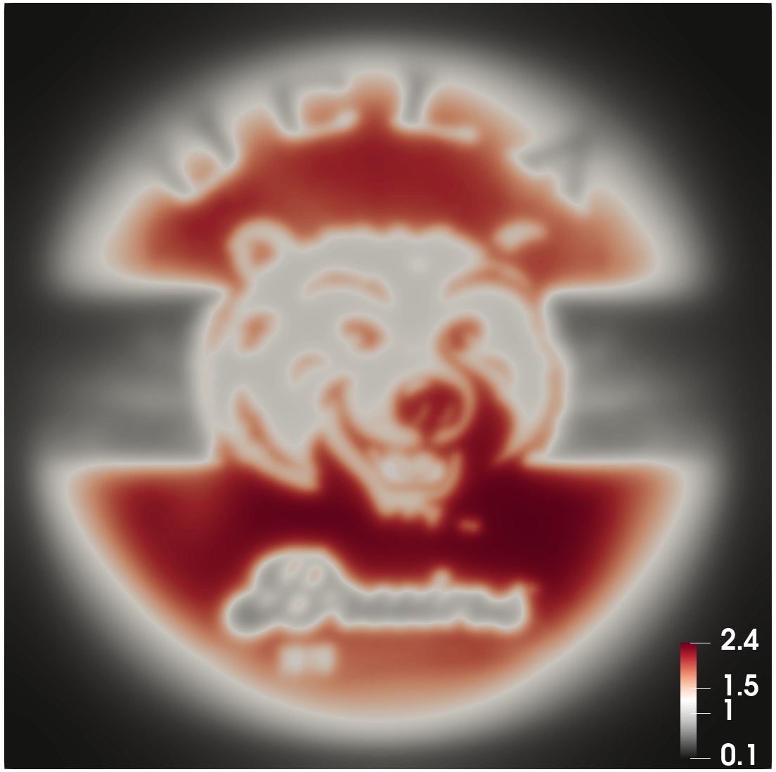
(c) Case 3: $A(\rho)=0.01/\rho$. ND $\rightarrow$ UCLA

Figure 6: Example 4.4. Initial density: ND. Terminal density: UCLA. Snapshots of $\rho$ at $t=$ 0.1,0.3,0.5,0.7,0.9 (left to right).

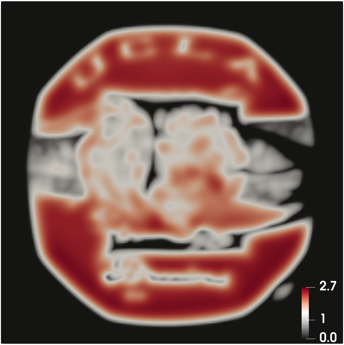
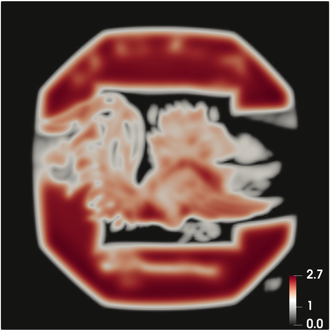
(a) Case 1: $A(\rho)=0$. UCLA $\rightarrow$ USC

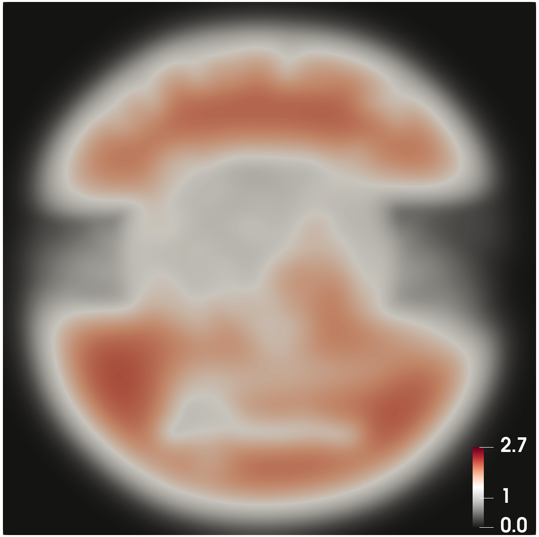
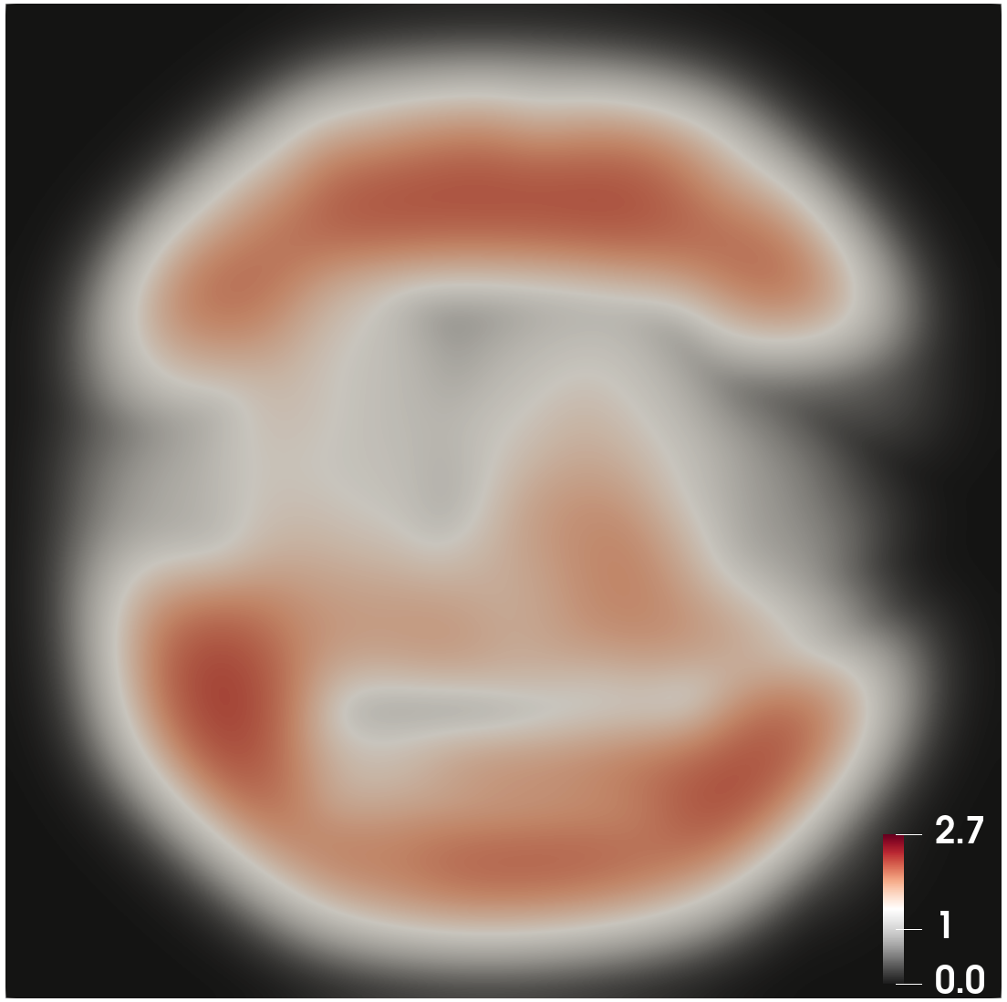
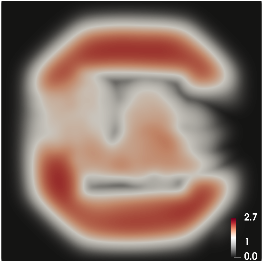
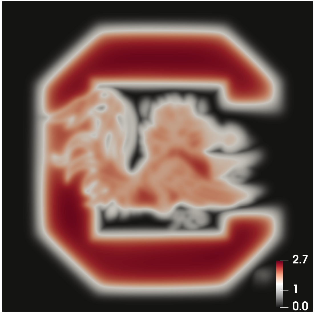
(b) Case 2: $A(\rho)=0.01\rho\log(\rho)$. UCLA $\rightarrow$ USC

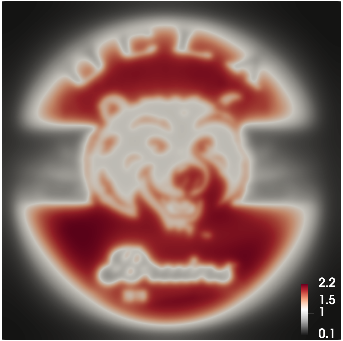
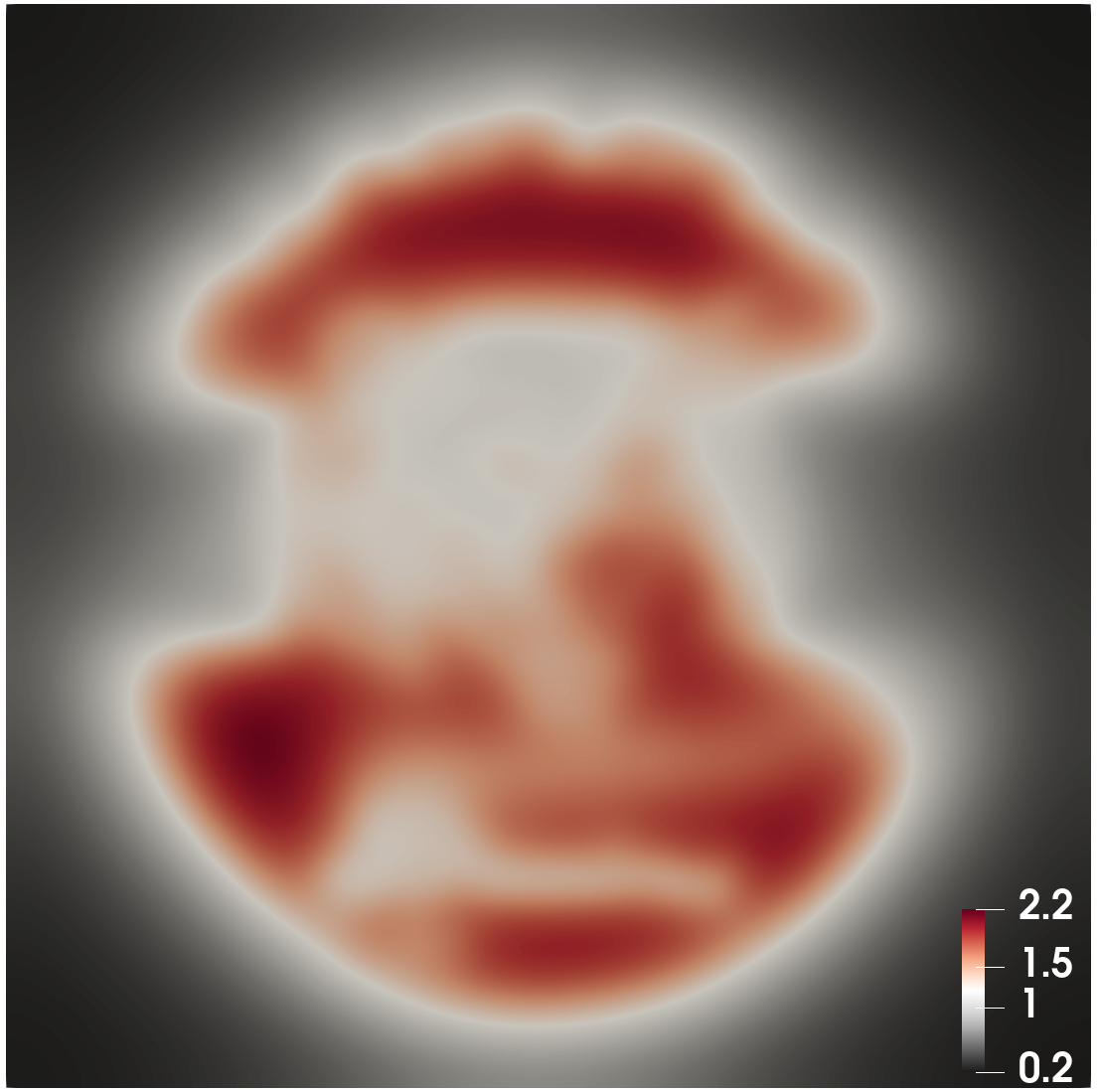
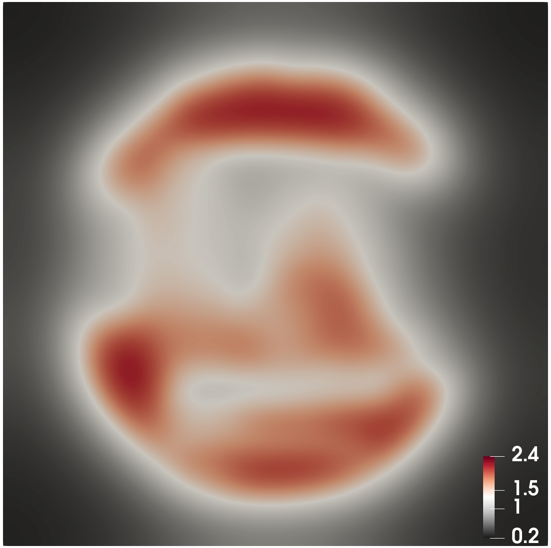
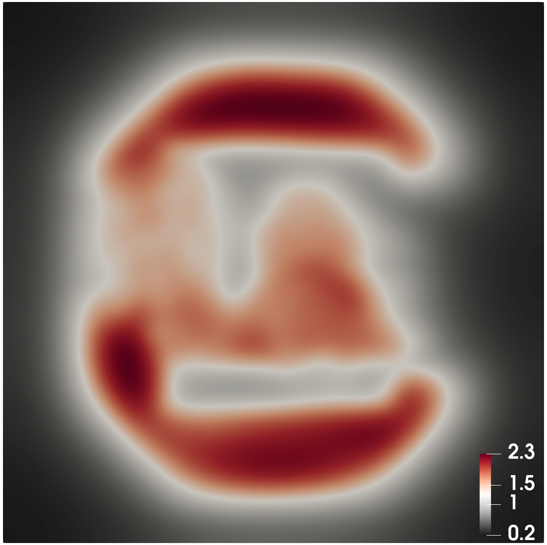
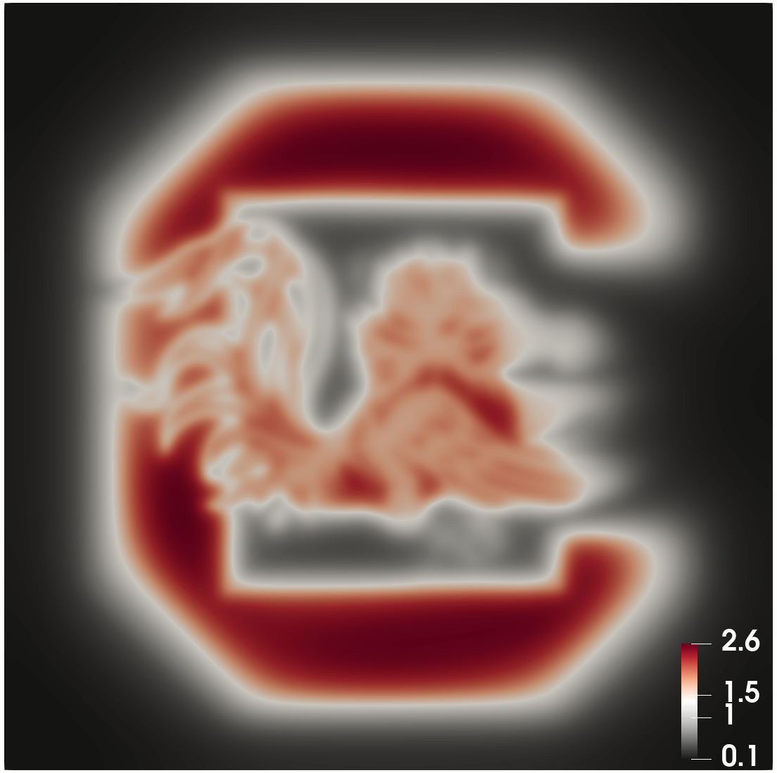
(c) Case 3: $A(\rho)=0.01/\rho$. UCLA $\rightarrow$ USC

Figure 7: Example 4.4. Initial density: UCLA. Terminal density: USC. Snapshots of $\rho$ at $t=$ 0.1,0.3,0.5,0.7,0.9 (left to right).

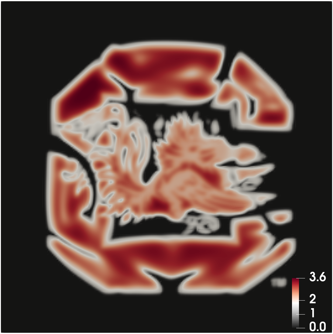
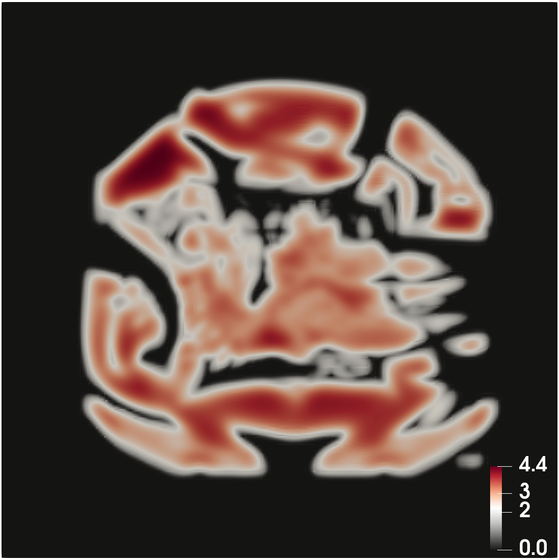
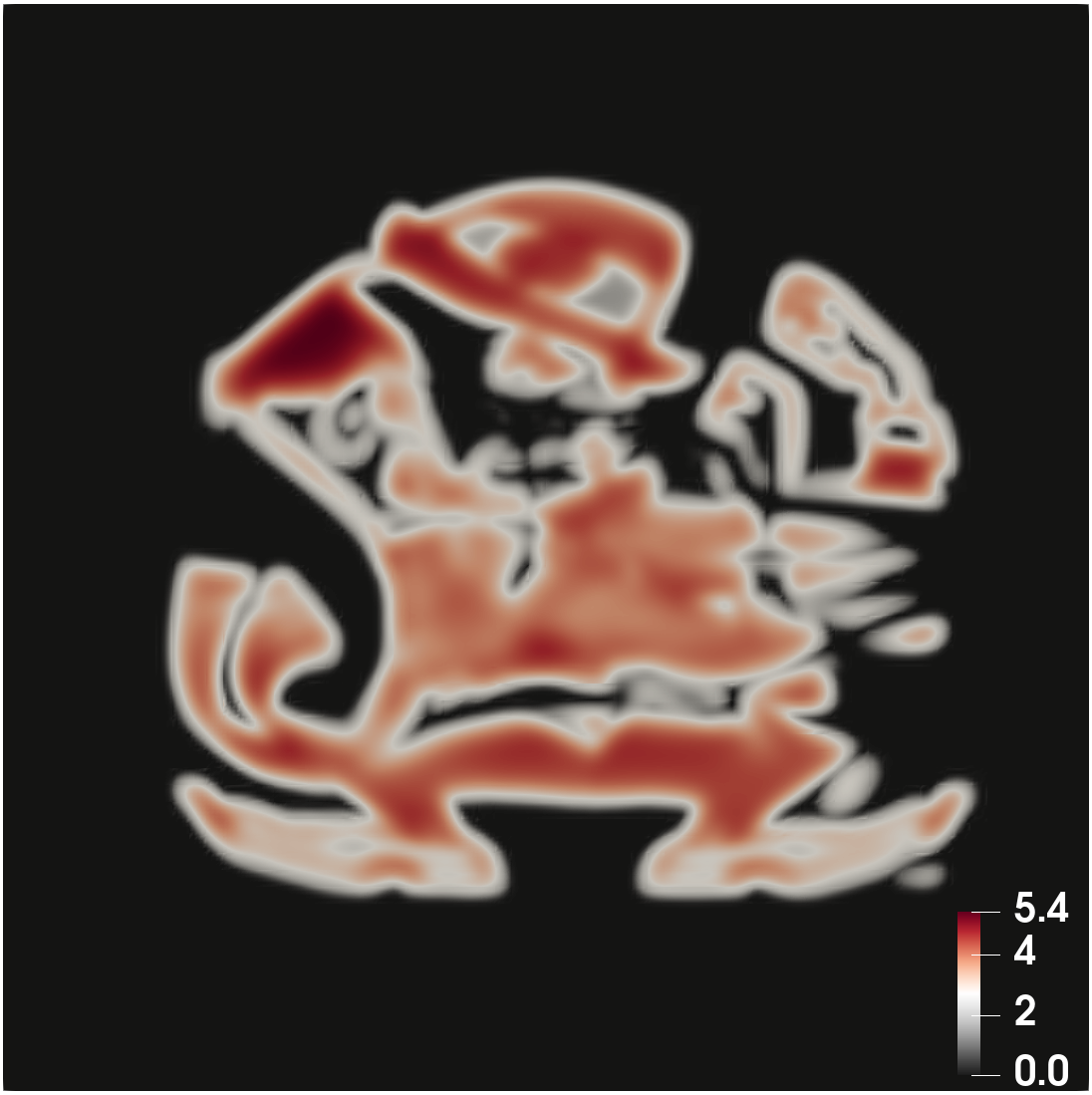
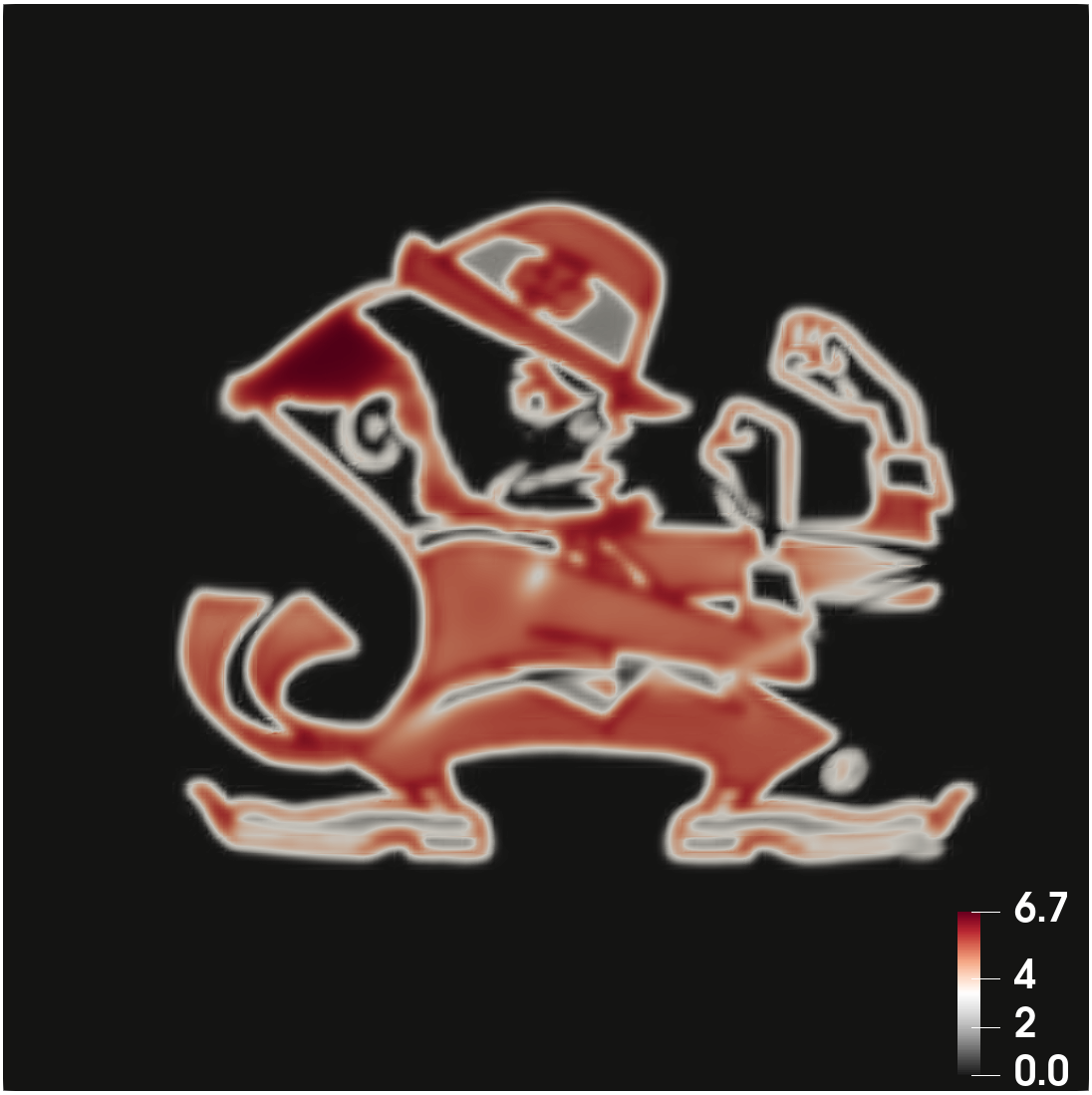
(a) Case 1: $A(\rho)=0$. USC $\rightarrow$ ND

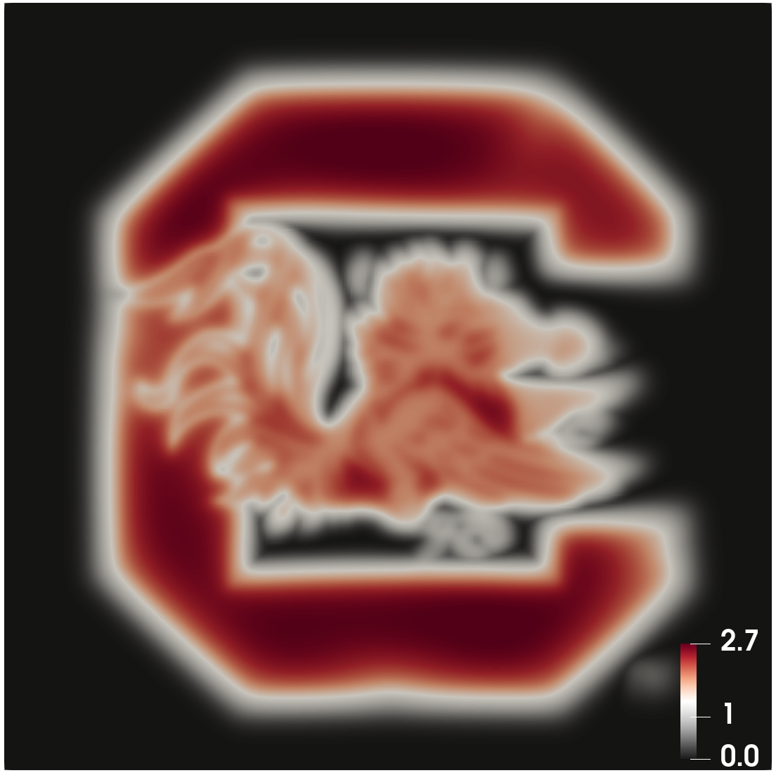
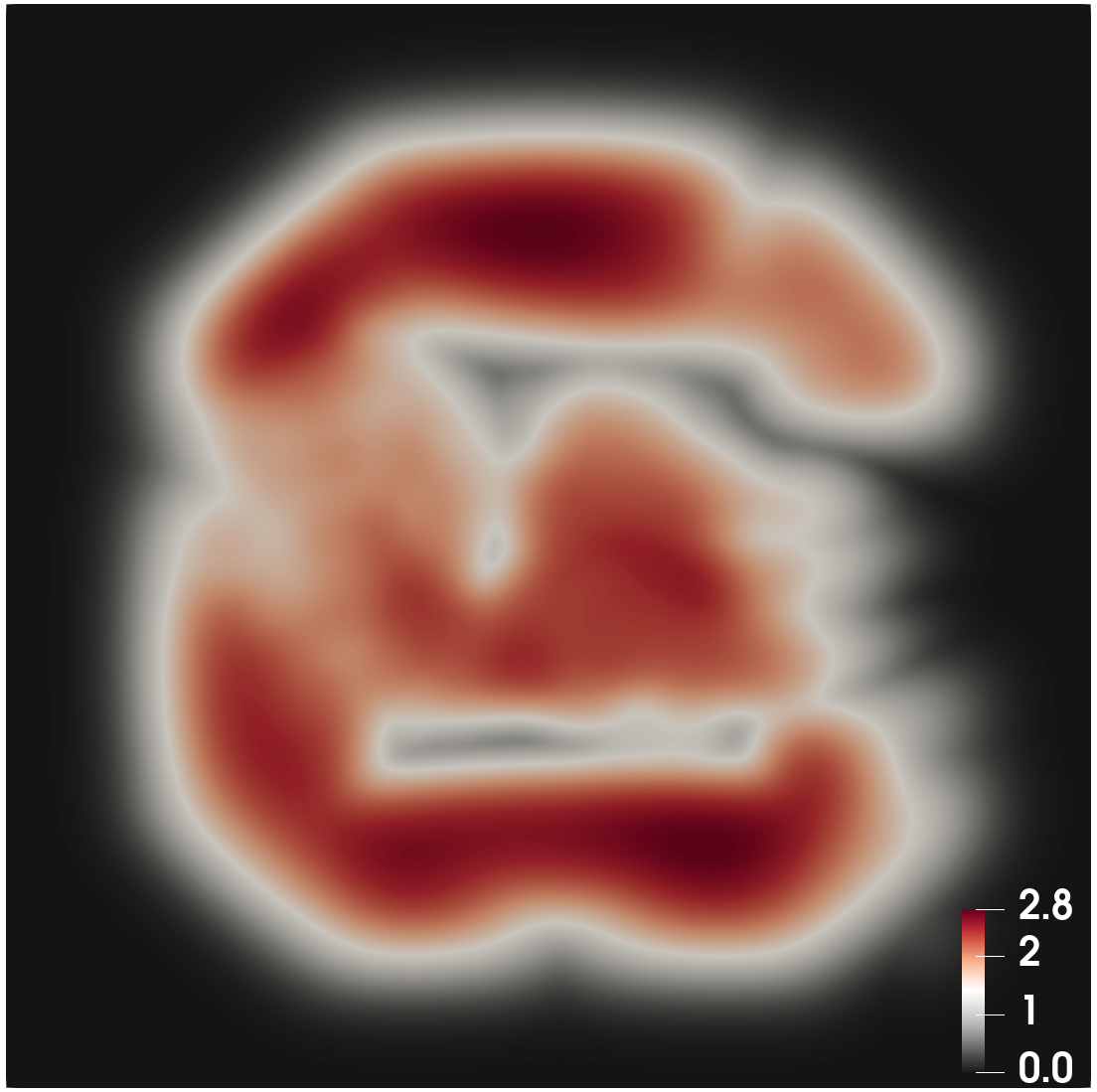
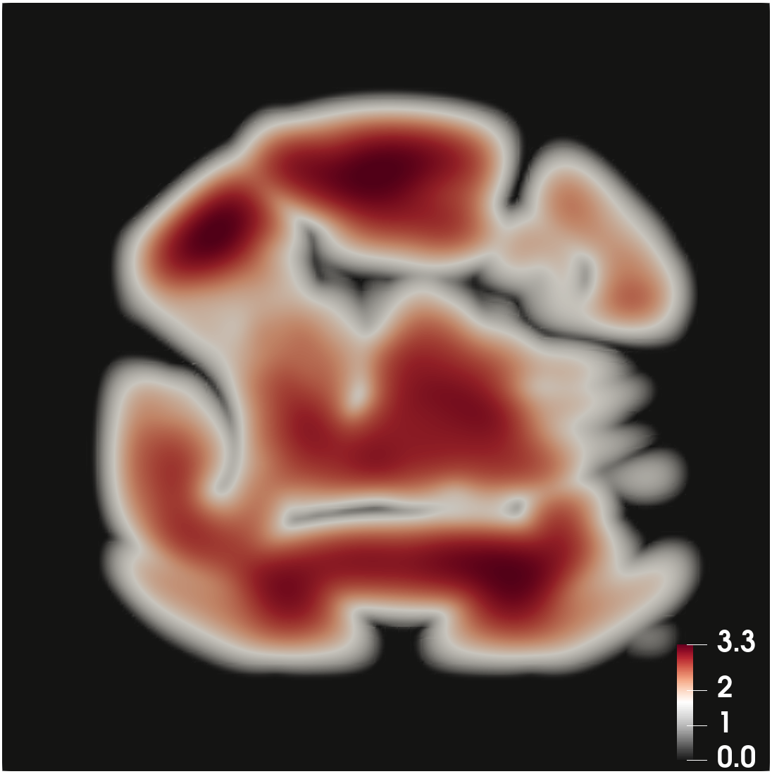
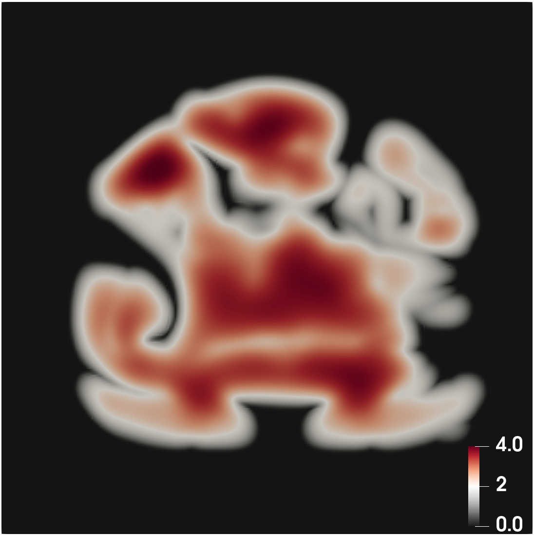
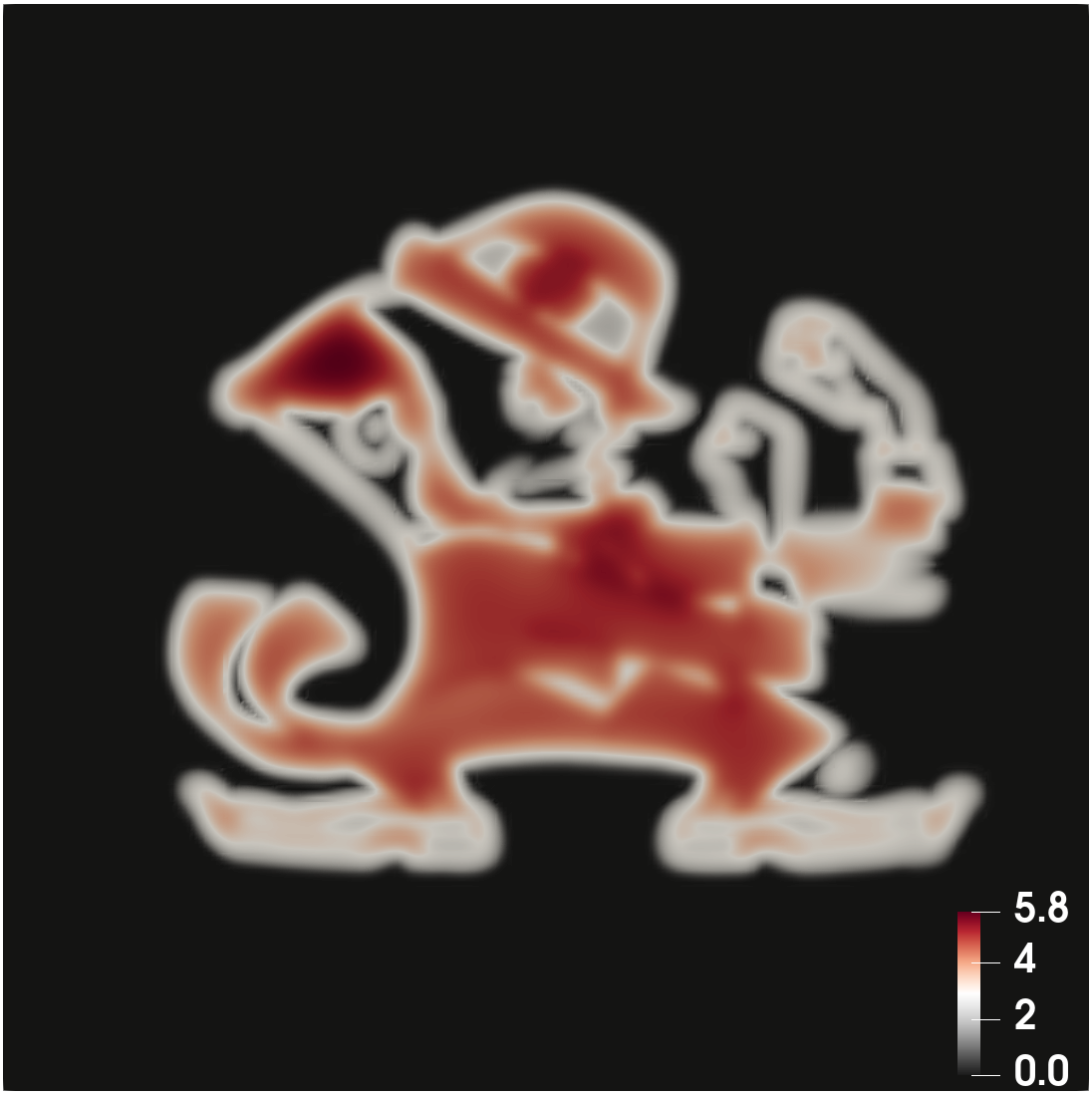
(b) Case 2: $A(\rho)=0.01\rho\log(\rho)$. USC $\rightarrow$ ND

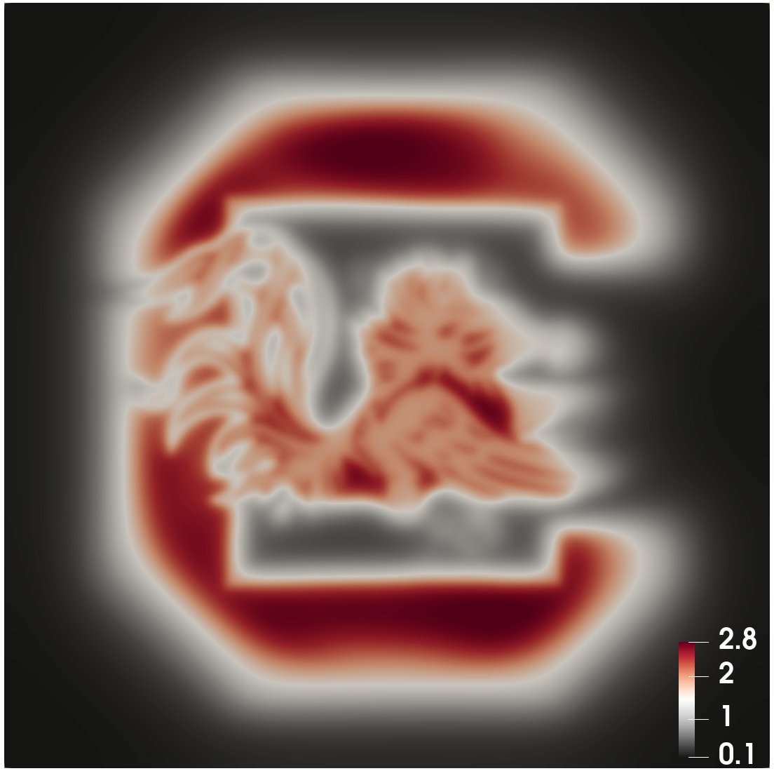
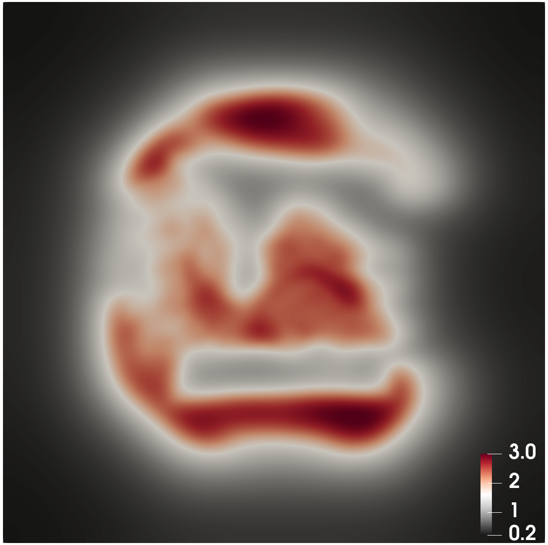
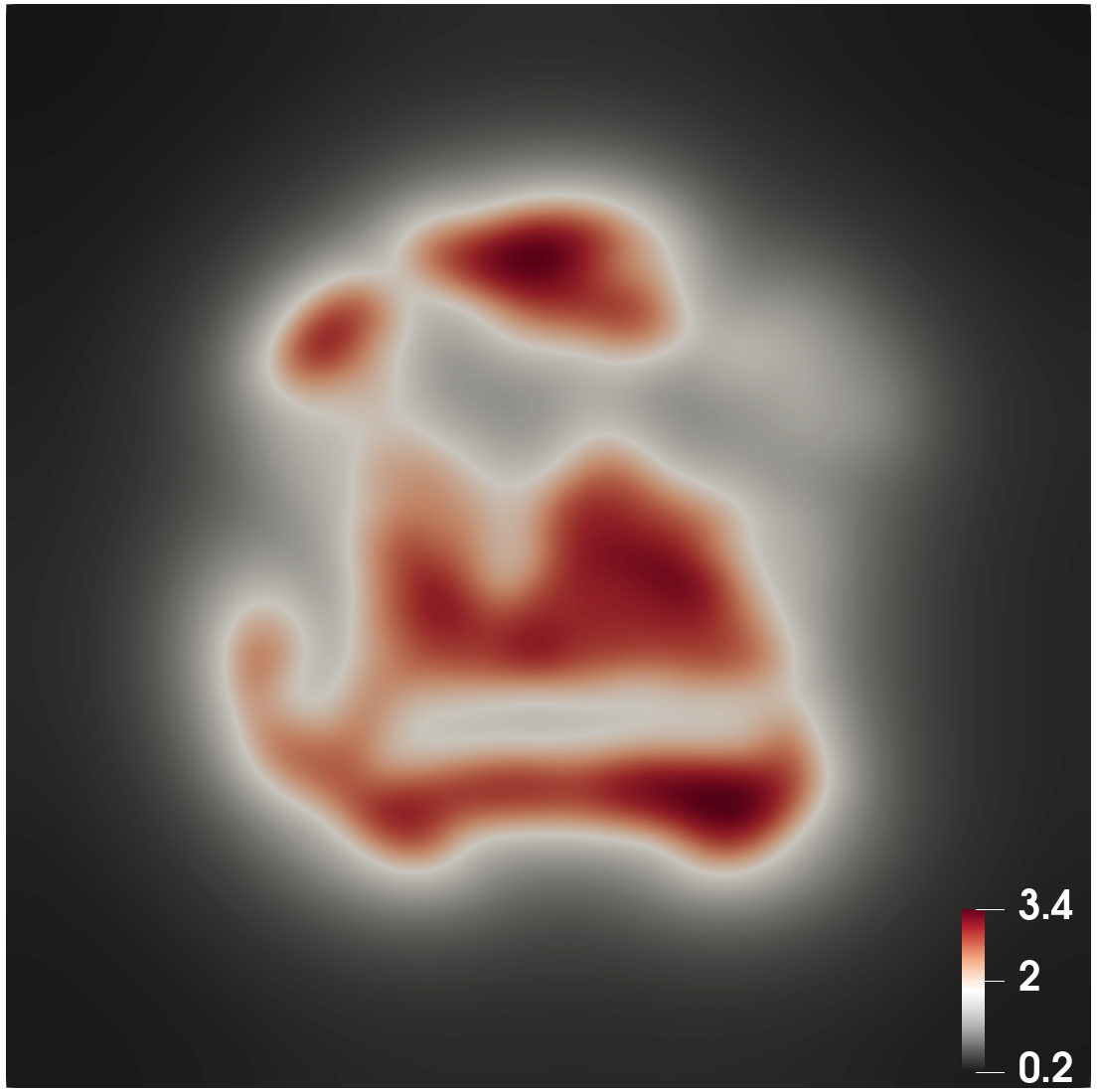
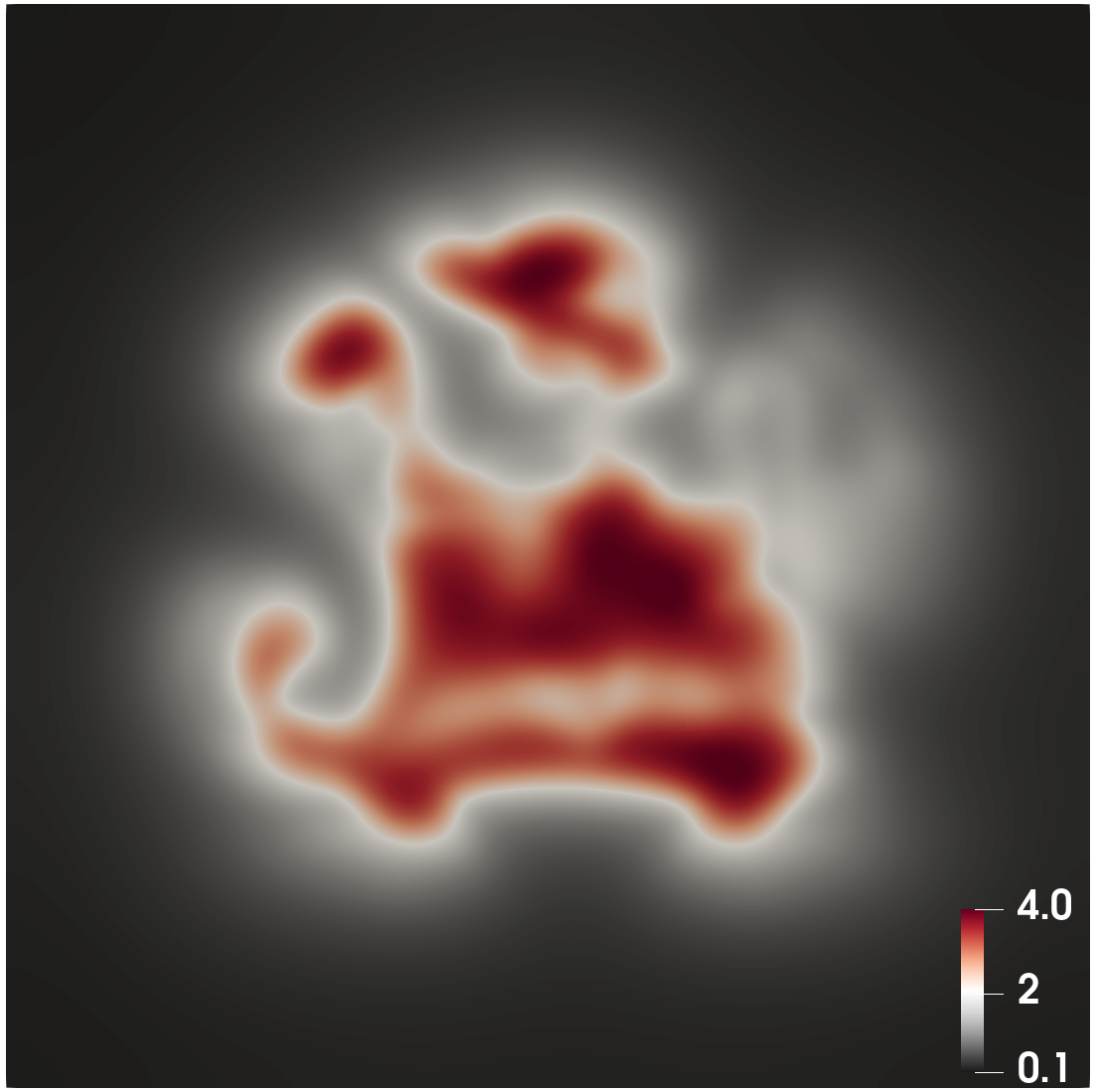
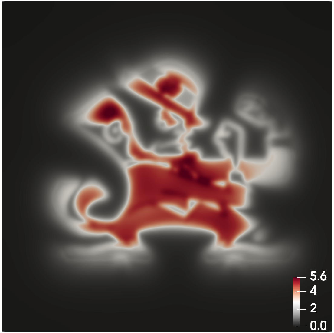
(c) Case 3: $A(\rho)=0.01/\rho$. USC $\rightarrow$ ND

Figure 8: Example 4.4. Initial density: USC. Terminal density: ND. Snapshots of $\rho$ at $t=$ 0.1,0.3,0.5,0.7,0.9 (left to right).

5 Conclusion

This paper applies high-order accurate finite element methods to compute optimal transport (OT) and mean field games (MFG). To our best knowledge, it is the first time to apply high order numerical methods in OT and MFGs. We verify the accuracy of algorithms through numerical examples. In future works, we shall investigate the numerical property of high-order accuracy FEM methods in OT and MFG-related dynamics. We expect they will have vast applications in computational physics, social science, biology modeling, pandemics control, and computer vision. We also expect to apply high order FEM in generalized mean field control formalisms to compute implicit-in-time fluid dynamics [35, 36, 37, 40].

References

- [1] Yves Achdou and Italo Capuzzo-Dolcetta, Mean field games: numerical methods, SIAM Journal on Numerical Analysis 48 (2010), no. 3, 1136–1162.
- [2] Yves Achdou and Mathieu Laurière, Mean field type control with congestion (ii): An augmented lagrangian method, Applied Mathematics & Optimization 74 (2016), no. 3, 535–578.
- [3] , Mean field games and applications: Numerical aspects, arXiv preprint arXiv:2003.04444 (2020).
- [4] Sudhanshu Agrawal, Wonjun Lee, Samy Wu Fung, and Levon Nurbekyan, Random features for high-dimensional nonlocal mean-field games, Journal of Computational Physics 459 (2022), 111136.
- [5] Roman Andreev, Preconditioning the augmented Lagrangian method for instationary mean field games with diffusion, SIAM J. Sci. Comput. 39 (2017), no. 6, A2763–A2783. MR 3731033
- [6] Alexander Aurell and Boualem Djehiche, Mean-field type modeling of nonlocal crowd aversion in pedestrian crowd dynamics, SIAM Journal on Control and Optimization 56 (2018), no. 1, 434–455.
- [7] Fabio Bagagiolo and Dario Bauso, Mean-field games and dynamic demand management in power grids, Dynamic Games and Applications 4 (2014), 155–176.
- [8] J.-D. Benamou, G. Carlier, and F. Santambrogio, Variational mean field games, Active particles. Vol. 1. Advances in theory, models, and applications, Model. Simul. Sci. Eng. Technol., Birkhäuser/Springer, Cham, 2017, pp. 141–171. MR 3644590
- [9] Jean-David Benamou and Yann Brenier, A numerical method for the optimal time-continuous mass transport problem and related problems, Contemporary mathematics 226 (1999), 1–12.
- [10] , A computational fluid mechanics solution to the monge-kantorovich mass transfer problem, Numerische Mathematik 84 (2000), no. 3, 375–393.
- [11] Jean-David Benamou and Guillaume Carlier, Augmented Lagrangian methods for transport optimization, mean field games and degenerate elliptic equations, J. Optim. Theory Appl. 167 (2015), no. 1, 1–26. MR 3395203
- [12] L. Briceño Arias, D. Kalise, Z. Kobeissi, M. Laurière, Á. Mateos González, and F. J. Silva, On the implementation of a primal-dual algorithm for second order time-dependent mean field games with local couplings, CEMRACS 2017—numerical methods for stochastic models: control, uncertainty quantification, mean-field, ESAIM Proc. Surveys, vol. 65, EDP Sci., Les Ulis, 2019, pp. 330–348. MR 3968547
- [13] G. Buttazzo, C. Jimenez, and E. Oudet, An optimization problem for mass transportation with congested dynamics, SIAM J. Control Optim. 48 (2009), no. 3, 1961–1976. MR 2516195
- [14] P. Cardaliaguet, Notes on mean field games, 2013, https://www.ceremade.dauphine.fr/ cardaliaguet/.
- [15] Pierre Cardaliaguet and Saeed Hadikhanloo, Learning in mean field games: the fictitious play, ESAIM: Control, Optimisation and Calculus of Variations 23 (2017), no. 2, 569–591.
- [16] Elisabetta Carlini and Francisco J Silva, A fully discrete semi-lagrangian scheme for a first order mean field game problem, SIAM Journal on Numerical Analysis 52 (2014), no. 1, 45–67.
- [17] René Carmona, Jean-Pierre Fouque, and Li-Hsien Sun, Mean field games and systemic risk, Communications in Mathematical Sciences 13 (2015), no. 4, 911–933.
- [18] Philippe Casgrain and Sebastian Jaimungal, Mean-field games with differing beliefs for algorithmic trading, Mathematical Finance 30 (2020), no. 3, 995–1034.
- [19] Kai Cui and Heinz Koeppl, Approximately solving mean field games via entropy-regularized deep reinforcement learning, International Conference on Artificial Intelligence and Statistics, PMLR, 2021, pp. 1909–1917.
- [20] Michel Fortin and Roland Glowinski, Augmented Lagrangian methods, Studies in Mathematics and its Applications, vol. 15, North-Holland Publishing Co., Amsterdam, 1983, Applications to the numerical solution of boundary value problems, Translated from the French by B. Hunt and D. C. Spicer. MR 724072
- [21] Diogo A. Gomes and J. Saúde, Mean field games models—a brief survey, Dyn. Games Appl. 4 (2014), no. 2, 110–154. MR 3195844
- [22] Olivier Guéant, Jean-Michel Lasry, and Pierre-Louis Lions, Mean field games and applications, Paris-Princeton Lectures on Mathematical Finance 2010, Lecture Notes in Math., vol. 2003, Springer, Berlin, 2011, pp. 205–266. MR 2762362
- [23] Xin Guo, Anran Hu, Renyuan Xu, and Junzi Zhang, A general framework for learning mean-field games, Mathematics of Operations Research (2022).
- [24] Saeed Hadikhanloo and Francisco J Silva, Finite mean field games: fictitious play and convergence to a first order continuous mean field game, Journal de Mathématiques Pures et Appliquées 132 (2019), 369–397.
- [25] Minyi Huang, Roland P Malhamé, Peter E Caines, et al., Large population stochastic dynamic games: closed-loop mckean-vlasov systems and the nash certainty equivalence principle, Communications in Information & Systems 6 (2006), no. 3, 221–252.
- [26] Noureddine Igbida and Van Thanh Nguyen, Augmented Lagrangian method for optimal partial transportation, IMA J. Numer. Anal. 38 (2018), no. 1, 156–183. MR 3800018
- [27] Arman C Kizilkale, Rabih Salhab, and Roland P Malhamé, An integral control formulation of mean field game based large scale coordination of loads in smart grids, Automatica 100 (2019), 312–322.
- [28] Aimé Lachapelle and Marie-Therese Wolfram, On a mean field game approach modeling congestion and aversion in pedestrian crowds, Transportation research part B: methodological 45 (2011), no. 10, 1572–1589.
- [29] Jean-Michel Lasry and Pierre-Louis Lions, Mean field games, Japanese journal of mathematics 2 (2007), no. 1, 229–260.
- [30] , Mean field games, Jpn. J. Math. 2 (2007), no. 1, 229–260. MR 2295621
- [31] Mathieu Lauriere, Numerical methods for mean field games and mean field type control, arXiv preprint arXiv:2106.06231 (2021).
- [32] Mathieu Laurière, Sarah Perrin, Sertan Girgin, Paul Muller, Ayush Jain, Theophile Cabannes, Georgios Piliouras, Julien Pérolat, Romuald Élie, Olivier Pietquin, et al., Scalable deep reinforcement learning algorithms for mean field games, International Conference on Machine Learning, PMLR, 2022, pp. 12078–12095.
- [33] Wonjun Lee, Siting Liu, Wuchen Li, and Stanley Osher, Mean field control problems for vaccine distribution, Research in the Mathematical Sciences 9 (2022), no. 3, 51.
- [34] Wonjun Lee, Siting Liu, Hamidou Tembine, Wuchen Li, and Stanley Osher, Controlling propagation of epidemics via mean-field control, SIAM Journal on Applied Mathematics 81 (2021), no. 1, 190–207.
- [35] Wuchen Li, Wonjun Lee, and Stanley Osher, Computational mean-field information dynamics associated with reaction-diffusion equations, Journal of Computational Physics 466 (2022), 111409.
- [36] Wuchen Li, Siting Liu, and Stanley Osher, Controlling conservation laws i: entropy-entropy flux, arXiv:2111.05473 (2021).
- [37] , Controlling conservation laws ii: Compressible navier–stokes equations, Journal of Computational Physics 463 (2022), 111264.
- [38] Alex Tong Lin, Samy Wu Fung, Wuchen Li, Levon Nurbekyan, and Stanley J Osher, Alternating the population and control neural networks to solve high-dimensional stochastic mean-field games, Proceedings of the National Academy of Sciences 118 (2021), no. 31, e2024713118.
- [39] Siting Liu, Matthew Jacobs, Wuchen Li, Levon Nurbekyan, and Stanley J Osher, Computational methods for first-order nonlocal mean field games with applications, SIAM Journal on Numerical Analysis 59 (2021), no. 5, 2639–2668.
- [40] Siting Liu, Stanley Osher, Wuchen Li, and Chi-Wang Shu, A primal-dual approach for solving conservation laws with implicit in time approximations, Journal of Computational Physics 472 (2023), 111654.
- [41] Alessio Porretta, On the planning problem for a class of mean field games, Comptes Rendus Mathematique 351 (2013), no. 11-12, 457–462.
- [42] Lars Ruthotto, Stanley J Osher, Wuchen Li, Levon Nurbekyan, and Samy Wu Fung, A machine learning framework for solving high-dimensional mean field game and mean field control problems, Proceedings of the National Academy of Sciences 117 (2020), no. 17, 9183–9193.
- [43] J. Schöberl, C++11 Implementation of Finite Elements in NGSolve, 2014, ASC Report 30/2014, Institute for Analysis and Scientific Computing, Vienna University of Technology.
- [44] F. D. Witherden and P. E. Vincent, On the identification of symmetric quadrature rules for finite element methods, Comput. Math. Appl. 69 (2015), no. 10, 1232–1241. MR 3333661
- [45] Jiajia Yu, Rongjie Lai, Wuchen Li, and Stanley Osher, Computational mean-field games on manifolds, arXiv:2206.01622 (2022).
- [46] Linbo Zhang, Tao Cui, and Hui Liu, A set of symmetric quadrature rules on triangles and tetrahedra, J. Comput. Math. 27 (2009), no. 1, 89–96. MR 2493559